Scalable Estimation of Multinomial Response Models with Uncertain Consideration Sets

Abstract

A standard assumption in the fitting of unordered multinomial response models for $J$ mutually exclusive nominal categories, on cross-sectional or longitudinal data, is that the responses arise from the same set of $J$ categories between subjects. However, when responses measure a choice made by the subject, it is more appropriate to assume that the distribution of multinomial responses is conditioned on a subject-specific consideration set, where this consideration set is drawn from the power set of $\{1,2,\ldots,J\}$. Because the cardinality of this power set is exponential in $J$, estimation is infeasible in general. In this paper, we provide an approach to overcoming this problem. A key step in the approach is a probability model over consideration sets, based on a general representation of probability distributions on contingency tables, which results in mixtures of independent consideration models. Although the support of this distribution is exponentially large, the posterior distribution over consideration sets given parameters is typically sparse, and is easily sampled in an MCMC scheme. We show posterior consistency of the parameters of the conditional response model and the distribution of consideration sets. The effectiveness of the methodology is documented in simulated longitudinal data sets with $J=100$ categories and real data from the cereal market with $J=68$ brands.

Keywords: Multinomial response, Bayesian computation, Dirichlet process mixture, Markov chain Monte Carlo

1 Introduction

In the generic multinomial/polychotomous models for $J$ mutually exclusive nominal categories/items in panel/longitudinal data settings, suppose $n$ independent categorical random variables $Y_{1t},\ldots,Y_{nt}$ are observed at time $t$. Suppose the probability that $Y_{it}$ falls into one of the $J$ categories, given parameters, random-effects, and covariates is specified independently over $t$ by the random-effects logit model:

$$\Pr(Y_{it}=j|\bm{\beta},\bm{b}_{i},\bm{\omega}_{it},\mathcal{C}_{i})=\begin{cases}\frac{\exp\left(V_{ijt}\right)}{\sum_{\ell\in\mathcal{C}_{i}}\exp\left(V_{i\ell t}\right)},&\text{if}\ j\in\mathcal{C}_{i}\\ 0,&\text{otherwise,}\end{cases}$$ (1)

for $j=1,\ldots,J$, where $V_{ijt}=\bm{x}_{ijt}^{\prime}\bm{\beta}+\bm{z}_{ijt}^{\prime}\bm{b}_{i}$, $\bm{x}_{ijt}\in\mathbb{R}^{d_{x}}$ and $\bm{z}_{ijt}\in\mathbb{R}^{d_{z}}$ are covariates with $\bm{\omega}_{it}=(\bm{x}_{ijt}^{\prime},\bm{z}_{ijt}^{\prime})^{\prime}$ and $\bm{\omega}_{it}=(\bm{\omega}_{i11}^{\prime},\ldots,\bm{\omega}_{iJt}^{\prime})^{\prime}$, $\bm{\beta}$ is the vector of common fixed-effects, and the random-effects $\bm{b}_{i}$ are distributed iid according to the multivariate normal distribution with mean vector $\bm{0}$ and covariance matrix $\bm{D}$, $N_{d_{z}}(\bm{0},\bm{D})$. The subset $\mathcal{C}_{i}$ of $\mathcal{J}=\{1,\ldots,J\}$ denotes the consideration set of the $i$th subject. The standard practice is to assume $\mathcal{C}_{i}=\mathcal{J}$ for all $i=1,\ldots,n$, that is, subjects consider all the $J$ categories. However, in situations where subjects make a decision from the available alternatives, it can be more appropriate to assume that actual choices are conditioned on a consideration set that is a proper subset of $\mathcal{J}$. However, from the perspective of the statistician, the consideration set used by the subject $i$ is unobserved. This motivates a more general multinomial model in which the consideration sets are latent and heterogeneous between subjects (Manski, 1977, Ben-Akiva and Boccara, 1995, Chiang et al., 1998, Cattaneo et al., 2020, Barseghyan et al., 2021, Lu, 2022, Aguiar et al., 2023).

Let $\mathcal{C}$ denote the set of possible consideration sets. This is given by the power set of $\mathcal{J}$ minus the empty set. Thus, $\mathcal{C}$ is a set consisting of $J^{\ast}=2^{J}-1$ sets. Assume that a priori, the consideration set of subject $i$, $\mathcal{C}_{i}$, is drawn from a probability mass distribution $\Pr(\mathcal{C}_{i}=c)$, where $c\in\mathcal{C}$. Then, the probability that $Y_{it}$ takes the value $j$, conditioned on parameters, random effects, and covariates, but marginalized over the possible consideration sets, is given by

$$\sum_{c\in\mathcal{C}}\Pr(Y_{it}=j|\bm{\beta},\bm{b}_{i},\bm{\omega}_{it},c)\Pr(\mathcal{C}_{i}=c),$$ (2)

a $J^{\ast}$ component mixture of multinonomial logit probabilities. By virtue of the mixing, this is a more general model than the multinomial logit model. Although there are many variants in terms of the modeling details, it can be applied quite generally, for example, to marketing (Van Nierop et al., 2010, Kawaguchi et al., 2021), economics (Goeree, 2008), transportation science (Swait and Ben-Akiva, 1987, Paleti et al., 2021), and psychology (Traets et al., 2022). Ignoring consideration set heterogeneity, when it is present, is clearly inappropriate (Crawford et al., 2021), but incorporating it can improve predictions, as we show in an empirical application.

The key inferential challenge in dealing with the mixture model in (2) is the exponentially large support of the probability mass distribution $\Pr(\mathcal{C}_{i}=c)$, $c\in\mathcal{C}$. When $J$ is roughly less than thirty, the nonparametric Bayesian approach of Chiang et al. (1998) can be applied effectively. In this approach, the different consideration sets are placed in 1-1 correspondence with the integers $1,2,\ldots,J^{\ast}$ and assigned a priori unknown probabilities $\pi_{1},\pi_{2},\ldots,\pi_{J^{\ast}}$. These probabilities are modeled by a Dirichlet prior and estimated in an MCMC based estimation approach in which the latent consideration sets are sampled given the observations, parameters, and random-effects; the parameters of the multinomial logit model and random effects are sampled given the observations and the sampled consideration sets; and finally the unknown probabilities are sampled given the sampled consideration sets.

Alternatively, one can model the probability mass function over consideration sets parametrically. Let $q_{ij}$ denote the probability that subject $i$ considers alternative $j$, for $j=1,\ldots,J$. Then, assuming that the items are considered (and not considered) independently, we would have the following independent consideration model.

$$\Pr\left(\mathcal{C}_{i}=c|\bm{q}\right)=\prod_{j\in c}q_{ij}\prod_{j\notin c}\big{(}1-q_{ij}\big{)},$$ (3)

where $q_{ij}$ is the attention probability (inclusion probability) of subject $i$ for item $j$. Note that the cardinality of the support on the left-hand side above is $J^{*}$, while that of $\bm{q}$ is $J$. This is the approach in (Ben-Akiva and Boccara, 1995, Goeree, 2008, Manzini and Mariotti, 2014, Kawaguchi et al., 2021, Abaluck and Adams-Prassl, 2021). One can go further along these lines and suppose that  $q_{ij}=\exp\left(\bm{a}_{ij}^{\prime}\bm{\theta}\right)/\left[1+\exp\left(\bm{a}_{ij}^{\prime}\bm{\theta}\right)\right]$, where $\bm{a}_{ij}$ is a vector of observable characteristics and $\bm{\theta}$ measures the sensitivity of category consideration with respect to these observables. Although attractive for modeling the large $J$ case, tractability comes at the cost of the restrictive independence assumption and a functional form assumption, and thus a greater risk of model misspecification (Crawford et al., 2021).

Another approach is considered by Van Nierop et al. (2010) where the elements of the consideration set are modeled as a vector of 0-1 binary variables. This vector is then modeled by a multivariate probit model (Chib and Greenberg, 1998). The approach is quite general, but inference can be challenging because the number of parameters in the correlation matrix of the multivariate probit model increases quadratically in $J$.

The purpose of this article is to introduce a new estimation approach for such models that is scalable in the number of alternatives. This approach does not impose restrictive assumptions on the a priori distribution of consideration sets. Two key elements characterize this approach. The first is a representation of the probability masses $\pi_{1},\pi_{2},\ldots,\pi_{J^{\ast}}$ in the approach of Chiang et al. (1998) in terms of mixtures of $J$ item-specific inclusion probabilities $q_{j}$. This representation is based on a result due to Dunson and Xing (2009). Because in this representation one takes a weighted average of products of item-specific inclusion/exclusion probabilities, we refer to this approach as a mixture of independent consideration models. It should be noted that in our application the consideration sets are latent, which makes the setting different from that of Dunson and Xing (2009) where the categorical variables are observed. The second element is the fact that the posterior distribution of consideration sets is, in general, sparse. This sparsity is a consequence of the fact that consideration sets that do not contain actual responses of the given subject must necessarily have zero posterior probability, first noted and exploited in Chiang et al. (1998). Posterior sparsity simplifies the MCMC-based estimation approach. Our theoretical derivations indicate posterior consistency of the parameters in the conditional response model and the distribution of the consideration sets.

The remainder of the paper is organized as follows. Section 2 contains the details of the model. Section 3 considers the prior-posterior distribution, while Section 4 develops the approach to posterior computation. Section 5 presents numerical simulations. An application to a marketing data set is given in Section 6.

2 The approach

Assume that the data consists of a cross-section or a repeated cross sections of $n$ a priori i.i.d. subjects. At each time $t=1,\ldots,T_{i}$, the outcome $y_{it}$ on the subject $i$ is categorical, taking values in $\mathcal{J}=\{1,\ldots,J\}$. Each subject $i$ is associated with a consideration set $\mathcal{C}_{i}$, a subset of $\mathcal{J}$. The researcher observes the response $y_{it}$, but not $\mathcal{C}_{i}$. In this paper, the consideration sets $\{\mathcal{C}_{i}\}$ are assumed to be time-invariant, which facilitates inference and prediction by introducing sparsity in the posterior support of the consideration sets as well as consistent estimation of individual consideration sets as the time periods increase. However, our approach can be easily applied in a setting with time-varying consideration sets.

We model the distribution of the observed outcomes hierarchically. We specify a marginal model for $\{\mathcal{C}_{i}\}$ and a conditional random effects logit model in (1) for the outcomes given the consideration set. We adopt the logit specification for simplicity of implementation, but this is not a limiting factor because the marginal model of the outcomes is a generalized multinomial logit due to the mixing over the possible consideration sets.

2.1 The latent consideration sets

To fix notations, recall that we define $\mathcal{C}$ as the collection of all consideration sets, that is, the power set of $\mathcal{J}=\{1,\ldots,J\}$ minus the empty set. The consideration set of subject $i$ is an element of this power set. We denote it by $\mathcal{C}_{i}=c$, for $c\in\mathcal{C}$. For example, when $J=3$,

$$\mathcal{C}=\{\{1\},\{2\},\{3\},\{1,2\},\{1,3\},\{2,3\},\text{and}\,\{1,2,3\}\}$$

and $c$ refers to an element of this set. Furthermore, by $\bm{C}_{i}=(C_{i1},\ldots,C_{iJ})^{\prime}$, we mean a $J\times 1$ multivariate binary vector where $C_{ij}=1$ if the category $j$ is in the consideration set and $0$ otherwise. In the example of $J=3$, $\mathcal{C}_{i}=\{1\}$ is equivalent to $\bm{C}_{i}=(1,0,0)^{\prime}$, $\mathcal{C}_{i}=\{1,3\}$ is equivalent to $\bm{C}_{i}=(1,0,1)^{\prime}$ and $\mathcal{C}_{i}=\{1,2,3\}$ is equivalent to $\bm{C}_{i}=(1,1,1)^{\prime}$, etc. Below, we use the two notations interchangeably depending on the context. In passing, we note that researchers sometimes include an outside option in the model that is always considered by each subject. We can incorporate this into our framework by adding a $(J+1)$th category and fixing $C_{iJ+1}=1$ for all $i$.

Our goal is to put a probability distribution on $\mathcal{C}$ that is rich enough to accommodate dependencies while maintaining scalability. As in Chiang et al. (1998), we do not include covariates in the consideration set model because in the large $J$ case, the focus of this paper, a covariate-dependent model would be difficult to specify without increasing the risk of model misspecification.

2.2 Dimensionality reduction via parallel factor analysis

We now review the factor decomposition technique that we employ to specify the distribution over consideration sets. Dunson and Xing (2009) consider modeling large contingency tables that, for example, represent DNA sequences, each of which is defined as a collection of $J$ categorical variables, each having $d_{j}$ possible values $j=1,\ldots,J$, where $J$ is large. A realization of the contingency table can be expressed as a vector $(a_{1},\ldots,a_{J})^{\prime}$, where $a_{j}\in\{1,\ldots,d_{j}\}$ for $j=1,\ldots,J$. The true distribution of the contingency tables is a probability tensor $\bm{\pi}=\{\pi_{a_{1}a_{2}\cdots a_{J}},a_{j}=1,\ldots,d_{j},j=1,\ldots,J\}$, where $0\leq\pi_{a_{1}a_{2}\cdots a_{J}}\leq 1$ and $\sum_{a_{1}=1}^{d_{1}}\cdots\sum_{a_{J}=1}^{d_{J}}\pi_{a_{1}a_{2}\cdots a_{J}}=1$. Note that consideration sets can be seen as contingency tables with $d_{j}=2$ for all $j$. Generally, there are a large number of elements in the tensor $\bm{\pi}$, $d_{1}\times\cdots\times d_{J}$, when $J$ is large. Dunson and Xing (2009) show that $\bm{\pi}$ can be expressed as a finite mixture of rank 1 tensors. This decomposition is called a parallel factor analysis and represents the full structure of dependence among $J$ categorical variables as a weighted sum of independent models, thus reducing the number of parameters to something only linear in $J$. We describe this result for the special case that corresponds to the modeling of consideration sets.

Lemma 1 (Exact matching of consideration set probabilities).

Let $\bm{\pi}$ be a distribution of consideration sets. That is, it is a collection of probabilities $\{\pi_{c}=\Pr\left(\mathcal{C}_{i}=c\right):c\in\mathcal{C}\}$, where $0\leq\pi_{c}\leq 1$ and $\sum_{c\in\mathcal{C}}\pi_{c}=1$. Then there are $K\in\mathbb{Z}^{+}$, $\bm{\omega}=(\omega_{1},\ldots,\omega_{K})\in\Delta^{K-1},$ $\bm{q}_{h}=(q_{h1},\ldots,q_{hJ})^{\prime},\quad h=1,\ldots,K,\quad q_{hj}\in[0,1]$ such that for each $c\in\mathcal{C}$,

$$\pi_{c}=\sum_{h=1}^{K}\omega_{h}\left\{\prod_{j\in c}q_{hj}\prod_{j\notin c}\big{(}1-q_{hj}\big{)}\right\}.$$ (4)

The lemma means that in order to describe an arbitrary dependence structure of consideration of $J$ categories, one can take a mixture of $K$ different independent consideration models (3). Although in each mixture component the attention probability of category $j$ is independently specified by $q_{hj}$ over $j=1,\ldots,J$, the lemma implies that marginally over the $K$ components, the mixture model can induce the dependence across the categories given by $\bm{\pi}$. Importantly, it indicates that the number of parameters associated with the distribution $\bm{\pi}$ can be reduced from $2^{J}-1$ to $K\times J+(K-1)$, which is linear in $J$ and therefore can help alleviate the dimensionality problem when $J$ is large. In summary, the lemma highlights that the mixture of independent consideration models can help us achieve scalability while maintaining the flexibility of the model for consideration sets and without recourse to misspecifying assumptions.

2.3 Infinite mixture of independent consideration models

Building on this result, we model the $J$-dimensional latent vectors $\{\bm{C}_{i}\}$ via a mixture of independent probabilities. The mixture is with respect to the vector of attention probabilities $\bm{q}=(q_{1},\ldots,q_{J})^{\prime}$. In practice, the number of components $K$ in (4) is unknown. To overcome this issue, following Dunson and Xing (2009), we use a Dirichlet process (DP) prior (Ferguson, 1973), which induces an infinite mixture model. We emphasize that our problem differs from Dunson and Xing (2009) in the sense that while the categorical variables (contingency tables) are observed in their paper, the corresponding objects (the consideration sets) are latent in the current problem. This requires some care in developing an estimation procedure, as we explain in Section 4.

We now describe our approach. Assume that $\{\bm{C}_{i}\}$ are iid with the density $f$, with $f({}\cdot{}|G)=\int\prod_{j=1}^{J}q_{j}^{C_{ij}}\left(1-q_{j}\right)^{1-C_{ij}}dG(\bm{q})$. Suppose that the discrete mixing distribution $G$ is modeled by a DP prior with a concentration parameter $\alpha$ and a specified base probability measure $G_{0}$ that depends on a hyperparameter $\underline{\bm{\phi}}_{q}$. Equivalently, via the stick-breaking construction (Sethuraman, 1994), we have the following representation: $\bm{C}_{i}$’s are iid with the density for the infinite mixture of independent consideration models:

$$\sum_{h=1}^{\infty}\omega_{h}\prod_{j=1}^{J}\left\{q_{hj}^{C_{ij}}\left(1-q_{hj}\right)^{1-C_{ij}}\right\},$$ (5)

where $\omega_{1}=V_{1},\omega_{h}=V_{h}\prod_{\ell<h}(1-V_{\ell}),h=2,\ldots,\infty,$ $V_{h}\overset{iid}{\sim}\text{Beta}(1,\alpha),h=1,\ldots,\infty$, and $\bm{q}_{h}\overset{iid}{\sim}G_{0}(\ \cdot\ |\underline{\bm{\phi}}_{q}),h=1,\ldots,\infty$, with $\bm{q}_{h}=(q_{h1},\ldots,q_{hJ})^{\prime}$ being the vector of attention probabilities specific to the component $h$. A priori, the first few weights dominate and cover most of the probability mass, which are then adjusted by the data. Although the model (5) includes infinitely many components, typically only very few distinct values for $\bm{q}_{h}$ are imputed.

For the baseline distribution $G_{0}$, we assume that $q_{hj}\sim G_{0j}$ independently for $j=1,\ldots,J$ and $h=1,\ldots,\infty$. Specifically, we assume that $q_{hj}\sim\text{Beta}(\underline{a}_{q_{j}},\underline{b}_{q_{j}})$, independently over $j=1,\ldots,J$, for $h=1,\ldots,\infty$, and define $\underline{\bm{\phi}}_{q}=(\underline{\bm{a}}_{q},\underline{\bm{b}}_{q})$ with $\underline{\bm{a}}_{q}=(\underline{a}_{q_{1}},\ldots,\underline{a}_{q_{J}})^{\prime}$ and $\underline{\bm{b}}_{q}=(\underline{b}_{q_{1}},\ldots,\underline{b}_{q_{J}})^{\prime}$. Note that $\underline{\bm{\phi}}_{q}=(\underline{\bm{a}}_{q},\underline{\bm{b}}_{q})$ are the hyperparameters that are chosen by the user. We will discuss this further in Section 5.

We complete the model specification by assuming the prior distribution for the DP concentration parameter $\alpha\sim\text{Gamma}(\underline{a}_{\alpha},\underline{b}_{\alpha}),$ where $(\underline{a}_{\alpha},\underline{b}_{\alpha})$ are the hyperparameters chosen by the user. For smaller values of $\alpha$, $\omega_{h}$ decreases toward zero more rapidly when the index $h$ increases, so that the prior favors a sparse representation with most of the weight on a few components. We allow the data to inform us about $\alpha$ and therefore an appropriate degree of sparsity, protecting against overfitting.

We show theoretically that, under mild conditions, our distribution over the consideration sets satisfies the Kullback–Leibler neighborhood property, a necessary condition for posterior consistency of the model parameters. In showing this result, we focus on the cross-sectional case, that is, when $T_{i}=1,\forall i=1,\ldots,n$. The result can be extended to the panel case, but at the expense of proof simplicity. Consequently, we drop the subscript $t$ in the presentation of the theoretical result below. Proofs of these results are outlined in the Appendix, while intermediate results that are used in the proofs are provided in the Supplemental Material.

Let $\bm{\theta}=\{\bm{\beta},\bm{D}\}$ denote the parameters in the response model. Also, recall that the distribution over the consideration sets is denoted by $\bm{\pi}=\{\pi_{c}:c\in\mathcal{C}\}$, where $0\leq\pi_{c}\leq 1$ and $\sum_{c\in\mathcal{C}}\pi_{c}=1$. Define the response probability conditional on the covariates $\bm{\omega}_{i}=\{(\bm{x}_{ij},\bm{z}_{ij})\in\mathbb{R}^{d_{x}+d_{z}}:j=1,\ldots,J\}$ taking some specific value $\bm{w}\in\mathbb{R}^{d_{x}+d_{z}}$ as: $p_{\bm{\theta},\bm{\pi}}(j|\bm{w})\equiv\sum_{c\in\mathcal{C}}\pi_{c}\Pr\left(Y_{i}=j|\bm{\theta},\bm{w},c),$ for $j\in\mathcal{J}=\{1,\ldots,J\}$ and $i=1,\ldots,n$, where $\Pr(Y_{i}=j|\bm{\theta},\bm{\omega}_{i},c)=\int\frac{\exp\left(V_{ij}\right)}{\sum_{\ell\in c}\exp\left(V_{i\ell}\right)}\phi(\bm{b}_{i}|\bm{0},\bm{D})d\bm{b}_{i}$ if $j\in c$ and $0$ otherwise, where $V_{ij}=\bm{x}_{ij}^{\prime}\bm{\beta}+\bm{z}_{ij}^{\prime}\bm{b}_{i}$. The data set contains responses $y_{i}$ and covariates $\bm{w}_{i}$: $\bm{D}^{n}=\{(y_{i},\bm{w}_{i}):i=1,\ldots,n\}$. The covariates $\bm{w}_{i}$ are iid and follow an unknown distribution with density $g^{*}$ with support $\mathcal{W}\subset\mathbb{R}^{J(d_{x}+d_{z})}$. We do not model the covariate distribution. Conditional on the covariates, the responses are generated from the collection of the data-generating response probabilities $\bm{p}^{*}=\{p_{\bm{\theta}^{*},\bm{\pi}^{*}}(j|\bm{w})\}_{j\in\mathcal{J},\bm{\omega}\in\mathcal{W}}$, where $\bm{\theta}^{*}$ and $\bm{\pi}^{*}=\{\pi^{*}_{c}:c\in\mathcal{C}\}$ denote the true data-generating values of the response model parameter as well as the probability mass function of consideration sets. Let $F_{0}$ be the data-generating density of the data $(y_{i},\bm{w}_{i})$.

Given a $K\in\mathbb{Z}^{+}$, define $\bm{\phi}_{1K}=(\omega_{h},\bm{q}_{h}:h=1,\ldots,K)$, the collection of all component-specific parameters, where $\bm{q}_{h}=(q_{h1},\ldots,q_{hJ})^{\prime}.$ Given $(K,\bm{\phi}_{1K})$, define the model induced probability for a consideration set $c\in\mathcal{C}$: $\pi(c|K,\bm{\phi}_{1K})=\sum_{h=1}^{K}\omega_{h}\prod_{j\in c}q_{hj}\prod_{j\notin c}(1-q_{hj}).$ For $\varepsilon>0$, define a Kullback-Leibler neighborhood of $\bm{p}^{*}$ as

$$KL_{\varepsilon}(\bm{p}^{*})=\left\{(\bm{\theta},\bm{\pi}):\int\sum_{j=1}^{J}\log\left(\frac{p_{\bm{\theta}^{*},\bm{\pi}^{*}}(j|\bm{w})}{p_{\bm{\theta},\bm{\pi}}(j|\bm{w})}\right)p_{\bm{\theta}^{*},\bm{\pi}^{*}}(j|\bm{w})g^{*}(\bm{w})d\bm{w}<\varepsilon.\right\}.$$

It is essentially a set of $(\bm{\theta},\bm{\pi})$ that makes $p_{\bm{\theta},\bm{\pi}}$ close to $p_{\bm{\theta}^{*},\bm{\pi}^{*}}$.

Theorem 1.

Suppose: (i) $\mathcal{W}$ is compact, (ii) For each $j\in\mathcal{J}$, there is a consideration set $c_{j}\in\mathcal{C}$ such that $\pi^{*}_{c_{j}}>0$ and $\Pr(Y=j|\bm{\theta}^{*},\bm{w},c_{j})>0$ for all $\bm{w}\in\mathcal{W}$, and (iii) $\forall K\in\mathbb{Z}^{+},\bm{\phi}_{1K},\bm{\theta}$ and open neighborhoods $\Phi^{K}$ of $\bm{\phi}_{1K}$ and $\Theta$ of $\theta$, $\Pi(\bm{\theta}\in\Theta,\bm{\phi}_{1K}\in\Phi^{K})>0$. Then, under the prior specified, for all weak neighborhood $\mathcal{U}$ of $\bm{p}^{*}$, as $n\to\infty$, $\Pi\left(\mathcal{U}|\bm{D}^{n}\right)\to 1\text{ a.s. }F_{0}^{\infty}.$

The theorem states that asymptotically, the posterior converges in a sense that the model-induced response probability is consistent with the true data-generating counterpart. Theorem 2 of Dunson and Xing (2009) establishes the posterior consistency when the categorical variables are observed. In our setting, the consideration sets are latent and integrated out in the likelihood function. In the context of semiparametric estimation of dynamic discrete choice models, Norets and Shimizu (2022) obtained a similar result. Our proof strategy is similar, but different, due to the presence of random-effects, continuous covariates, and a different model. The compactness assumption (i) is common in Bayesian nonparametric estimation. Condition (ii) means that for each alternative, there is at least one consideration set that contains the alternative and has a positive probability under the true distribution $\bm{\pi}^{*}$, and the response probability conditional on this set is non-zero for that alternative. This is a reasonable assumption and implies that the true response probability $p_{\bm{\theta}^{*},\bm{\pi}^{*}}(j|\bm{w})$ is positive for all $(j,\bm{w})\in\mathcal{J}\times\mathcal{W}$. Note that condition (iii) of Theorem 1 is satisfied by our prior: the DP prior for $\omega_{h}$’s and the Beta prior for $q_{hj}$’s as shown by Dunson and Xing (2009).

3 Inference

3.1 Data structure

Let $\bm{Y}_{i}=(Y_{i1},\ldots,Y_{iT_{i}})^{\prime}$ and $\bm{y}_{i}=(y_{i1},\ldots,y_{iT_{i}})^{\prime}$ be the sequence of random responses made by unit $i$ over $T_{i}$ periods and its observed counterpart. Let $\bm{\omega}_{i}=(\bm{\omega}_{i1}^{\prime},\ldots,\bm{\omega}_{iT_{i}}^{\prime})^{\prime}$ be the covariates for the subject $i$ observed over time. Define

$$p(\bm{Y}_{i}=\bm{y}_{i}|\bm{\beta},\bm{b}_{i},\bm{\omega}_{i},\bm{C}_{i})=\prod_{t=1}^{T_{i}}\Pr(Y_{it}=y_{it}|\bm{\beta},\bm{b}_{i},\bm{\omega}_{it},\mathcal{C}_{i}),$$ (6)

where $\Pr(Y_{it}=y_{it}|\bm{\beta},\bm{b}_{i},\bm{\omega}_{it},\mathcal{C}_{i})$ is given by the random-effects logit model (1). Note that $\bm{C}_{i}$ is the conditioning variable on the left-hand side of this expression, while $\mathcal{C}_{i}$ is on the right-hand side. Although the two objects represent the same information, the $\bm{C}_{i}$ notation is easier to use when we discuss posterior sampling.

Let $\bm{Y}=\{\bm{Y}_{1},\ldots,\bm{Y}_{n}\}$ and $\bm{y}=\{\bm{y}_{1},\ldots,\bm{y}_{n}\}$ denote the random and observed sequences of the responses made by all units, and let $\bm{\omega}=\{\bm{\omega}_{1},\ldots,\bm{\omega}_{n}\}$ be the observed covariates. Then the likelihood conditional on the common fixed-effects $\bm{\beta}$, the random-effects $\bm{b}=(\bm{b}_{1},\ldots,\bm{b}_{n})^{\prime}$, the covariates $\bm{\omega}$, and the latent consideration sets $\bm{C}=(\bm{C}_{1},\ldots,\bm{C}_{n})$ is given by

$$p(\bm{Y}=\bm{y}|\bm{\beta},\bm{b},\bm{\omega},\bm{C})=\prod_{i=1}^{n}p(\bm{Y}_{i}=\bm{y}_{i}|\bm{\beta},\bm{b}_{i},\bm{\omega}_{i},\bm{C}_{i}).$$ (7)

We complete the model by specifying prior distributions for the parameters in the response model, namely $(\bm{\beta},\bm{D})$. We assume the following standard priors independently: $\bm{\beta}\sim N_{d_{x}}\left(\bm{0},\underline{\bm{V}}_{\beta}\right)$ and $\bm{D}^{-1}\sim\text{Wishart}\left(\underline{v},\underline{\bm{R}}\right)$, a normal distribution for $\bm{\beta}$, and an inverse Wishart distribution for $\bm{D}$ with degrees-of-freedom parameter $\underline{v}$ and scale matrix $\underline{\bm{R}}$. The hyperparameters $(\underline{\bm{V}}_{\beta},\underline{v},\underline{\bm{R}})$ are chosen by the user.

3.2 Posterior distribution

For the mixture model on the latent consideration sets $\bm{C}=(\bm{C}_{1},\ldots,\bm{C}_{n})$, let $S_{i}\in\{1,2,\ldots\}$ be the latent cluster assignment such that $C_{ij}|S_{i}=h\sim\text{Bernoulli}(q_{hj})$, independently $j=1,\ldots,J$, for $i=1,\ldots,n$. We have the latent consideration sets $\bm{C}$, the common fixed-effects $\bm{\beta}$, the random-effects $\bm{b}$, the corresponding covariance matrix $\bm{D}$, the DP parameters $\bm{V}=(V_{1},V_{2},\ldots)$ as well as $\bm{Q}=(\bm{q}_{1},\bm{q}_{2},\ldots)$, the DP cluster assignment variables $\bm{S}=(S_{1},\ldots,S_{n})$, and the DP concentration parameter $\alpha$. Then, from the Bayes theorem, we define the posterior density of interest to be

$$p\big{(}\bm{C}, \ \bm{S},\bm{V},\bm{Q},\alpha,\bm{\beta},\bm{b},\bm{D}\big{|}\bm{y},\bm{\omega}\big{)}\propto p\big{(}\bm{y}\big{|}\bm{\beta},\bm{b},\bm{\omega},\bm{C}\big{)}\cdot p(\bm{\beta},\bm{b},\bm{D})\cdot p\big{(}\bm{C},\bm{S},\bm{Q},\bm{V},\alpha\big{)}$$

$$=p\big{(}\bm{y}\big{|}\bm{\beta},\bm{b},\bm{\omega},\bm{C}\big{)}\cdot\pi(\bm{\beta})p(\bm{b}|\bm{D})\pi(\bm{D})\cdot p\big{(}\bm{C},\bm{S},\bm{Q},\bm{V},\alpha\big{)},$$ (8)

where the first term is the likelihood function given by (7) and $\pi(\cdot)$ denotes the prior density. Only the last term in (8) is associated with the DP model and

$$p\big{(}\bm{C},\bm{S},\bm{Q},\bm{V},\alpha\big{)} \propto p\big{(}\bm{C}|\bm{Q},\bm{S}\big{)}p\big{(}\bm{Q},\bm{V},\bm{S},\alpha\big{)}$$

$$\propto\left[\prod_{i=1}^{n}p\big{(}\bm{C}_{i}|\bm{q}_{S_{i}}\big{)}p\big{(}S_{i}|\bm{V}\big{)}\right]\cdot\left[\prod_{h=1}^{\infty}p\big{(}V_{h}|\alpha\big{)}p(\bm{q}_{h}|\underline{\bm{\phi}}_{q}\big{)}\right]\cdot\pi(\alpha),$$ (9)

where $p\big{(}\bm{C}_{i}|\bm{q}_{S_{i}}\big{)}$ is the product of densities for the independent Bernoulli distributions $\text{Bernoulli}(q_{S_{i}j})$ $j=1,\ldots,J$ , $p\big{(}S_{i}|\bm{V}\big{)}=\omega_{S_{i}}$, $p\big{(}V_{h}|\alpha\big{)}$ is the density of $\text{Beta}(1,\alpha)$, $p(\bm{q}_{h}|\underline{\bm{\phi}}_{q}\big{)}$ is the product of densities for the independent Beta distributions $\text{Beta}(\underline{a}_{q_{j}},\underline{b}_{q_{j}})$ $j=1,\ldots,J$, and $\pi(\alpha)$ is the prior density for $\alpha$. We apply the slice sampling approach (Walker, 2007) by augmenting the joint distribution with a sequence of auxiliary random variables $\bm{u}=(u_{1},\ldots,u_{n})$ that follow the uniform distribution on $(0,1)$, $u_{i}\sim\mathcal{U}(0,1)$, $i=1,\ldots,n$:

$$p(\bm{C},\bm{S},\bm{Q},\bm{V},\bm{u},\alpha)\propto\left[\prod_{i=1}^{n}p\big{(}\bm{C}_{i}|\bm{q}_{S_{i}}\big{)}I(u_{i}\leq\omega_{S_{i}})\right]\cdot\left[\prod_{h=1}^{\infty}p\big{(}V_{h}|\alpha\big{)}p(\bm{q}_{h}|\underline{\bm{\phi}}_{q}\big{)}\right]\cdot\pi(\alpha).$$ (10)

It is easy to show that we can recover (9) by integrating out $\bm{u}$ from (10). However, by introducing $\bm{u}$, one only has to choose labels $S_{i}$ in the finite set $\{h:\omega_{h}>u_{i}\}$.

4 Computation

Markov chain Monte Carlo (MCMC) methods can be applied to efficiently sample the posterior distribution. The algorithm we present is scalable and is constructed from simple and intuitive steps. Posterior inferences are based on the sample of draws produced by the algorithm. The posterior sample consists of $\{u_{i}^{(g)}\}$, $\{V_{h}^{(g)}\}$, $\{\bm{q}_{h}^{(g)}\}$, $\{S_{i}^{(g)}\},$ $\alpha^{(g)}$, $\big{\{}\bm{C}_{i}^{(g)}\big{\}}$, $\bm{\beta}^{(g)}$, $\big{\{}\bm{b}_{i}^{(g)}\big{\}}$, and $\bm{D}^{(g)}$ for $g=1,\ldots,G$, where $G$ is the number of MCMC draws (beyond a suitable burn-in). From the sample, we can compute posterior quantiles of different objects of interest, such as consideration probabilities $\Pr(C_{ij}=1)$, correlation of considerations $\Pr(C_{ij}=1\text{ and }C_{i\ell}=1)$ for $j\neq\ell$, the similarity matrix $\Pr(S_{i}=S_{i^{\prime}})$ for $i,i^{\prime}=1,\ldots,n$, marginal response probabilities $\Pr(Y_{it}=j|\bm{\omega}_{it})$, conditional response probabilities $\Pr(Y_{it}=j|\bm{\omega}_{it},\mathcal{C}_{i}=c)$, and predictive response probabilities.

4.1 Simulation of consideration sets

We now focus on sampling the conditional distribution of consideration sets. The other steps in the MCMC algorithm follow from standard calculations. The details are given in Section A of the Supplementary Material. From Equation (8), the full conditional distribution of $\bm{C}_{i}$ is

$$\pi(\bm{C}_{i}|\bm{\beta},\bm{b}_{i},\bm{q}_{S_{i}},S_{i},\bm{y}_{i},\bm{\omega}_{i})\propto\ p\big{(}\bm{Y}_{i}=\bm{y}_{i}\big{|}\bm{\beta},\bm{b}_{i},\bm{\omega}_{i},\bm{C}_{i}\big{)}\cdot\prod_{j=1}^{J}q_{S_{i}j}^{C_{ij}}(1-q_{S_{i}j})^{1-C_{ij}},$$ (11)

where the proportionality sign is with respect to $\bm{C}_{i}$, and the first term is defined in (6). Importantly, consideration sets that exclude any observed response made by the subject $i$ receive zero posterior probability (see Table 1 for an example). This is because the first term on the left-hand side of (11) is zero for these consideration sets. This desirable feature of our approach is based on Chiang et al. (1998). In contrast, in many existing methods, every consideration set receives a strictly positive probability, as pointed out by Crawford et al. (2021). Now, due to the independence structure in (11) over $j=1,\ldots,J$,

$$\pi(C_{ij}|\bm{C}_{i}\setminus\{j\},\bm{\beta},\bm{b}_{i},\bm{q}_{S_{i}},S_{i},\bm{y}_{i},\bm{\omega}_{i})\propto\ p\big{(}\bm{Y}_{i}=\bm{y}_{i}\big{|}\bm{\beta},\bm{b}_{i},\bm{\omega}_{i},\bm{C}_{i}\big{)}\cdot q_{S_{i}j}^{C_{ij}}(1-q_{S_{i}j})^{1-C_{ij}},$$ (12)

where $\bm{C}_{i}\setminus\{j\}$ denotes $\bm{C}_{i}$ without the coordinate $j$. To sample this distribution, we apply the Metropolis-Hastings (M-H) algorithm. Algorithm 1 shows an effective implementation.

Input: The current draws at the $g$th iteration $\big{\{}\bm{C}_{i}^{(g)}\big{\}},\{\bm{q}_{h}^{(g)}\},\{S_{i}^{(g)}=h\},\bm{\beta}^{(g)},\big{\{}\bm{b}_{i}^{(g)}\big{\}}$

Output: The updated consideration sets $\big{\{}\bm{C}_{i}^{(g+1)}\big{\}}$

for $i\in\{1,\ldots,n\}$ do

       for $j\in\{1,\ldots,J\}$ do

             1) Propose $\tilde{C}_{ij}\sim\text{Bernoulli}(q_{hj}^{(g)})$ and define $\bm{C}_{i}^{(1)}=(C_{i1}^{(g+1)},\ldots,C_{ij-1}^{(g+1)},\tilde{C}_{ij},C_{ij+1}^{(g)},\ldots,C_{iJ}^{(g)})^{\prime}$

             

             2) Accept $\tilde{C}_{ij}$ with probability

$$\min\left\{\frac{p\big{(}\bm{Y}_{i}=\bm{y}_{i}\big{|}\bm{\beta}^{(g)},\bm{b}_{i}^{(g)},\bm{\omega}_{i},\bm{C}_{i}^{(1)}\big{)}}{p\big{(}\bm{Y}_{i}=\bm{y}_{i}\big{|}\bm{\beta}^{(g)},\bm{b}_{i}^{(g)},\bm{\omega}_{i},\bm{C}^{(0)}_{i}\big{)}},1\right\},$$

where $\bm{C}_{i}^{(0)}=(C_{i1}^{(g+1)},\ldots,C_{ij-1}^{(g+1)},C_{ij}^{(g)},C_{ij+1}^{(g)},\ldots,C_{iJ}^{(g)})^{\prime}$.

             Otherwise, set $C_{ij}^{(g+1)}=C_{ij}^{(g)}$

      

Algorithm 1 M-H step for Sampling Consideration Sets

In Step 1) of Algorithm 1, we propose from a one-dimensional Bernoulli distribution. In Step 2), given the current $\bm{C}_{i}^{(0)}$, and the proposed $\bm{C}_{i}^{(1)}$, the acceptance probability is given by the ratio of the likelihood contributions of subject $i$. This M-H step is justified because $p\big{(}\bm{Y}_{i}=\bm{y}_{i}\big{|}\bm{\beta},\bm{b}_{i},\bm{\omega}_{i},\bm{C}_{i}\big{)}$ is uniformly bounded. See Chib and Greenberg (1995) (p330, ‘the third algorithm’) for more discussion. In practice, we implement these updates in random order in each MCMC iteration. Moreover, the computations involved can be done quickly by parallelizing the loop over the $n$ subjects.

We remark on some important aspects of this M-H step. Suppose that an alternative $j$ was not chosen by the subject $i$ in any period (otherwise, it must be in the consideration set for $i$ and $C_{ij}=1$). Depending on the current $C_{ij}^{(g)}$, and the proposed $\tilde{C}_{ij}$, there are four possible moves in the M-H step. First, if $\tilde{C}_{ij}=C_{ij}^{(g)}$, then the proposed value is accepted with probability one. Second, if $\tilde{C}_{ij}=0$ and $C_{ij}^{(g)}=1$, then the proposed value is also accepted with probability one. In other words, the algorithm “prefers” a smaller consideration set. This sparsity-inducing property is proven in the Supplementary Material. Last, when the proposed consideration set adds an alternative $j$ that is not in the current consideration set, that is, $\tilde{C}_{ij}=1$ and $C_{ij}^{(g)}=0$, the acceptance probability is between 0 and 1 and is determined by the likelihood ratio.

5 Numerical illustration

We now illustrate our theoretical findings under a small number of alternatives, $J=4$. This is because it is possible to enumerate all consideration sets when $J$ is small, which facilitates the presentation of the results. We also conducted a simulation study with $J=100$ and present the results in the Supplementary Material. We also demonstrate the scalability of our approach in the application with $J=68$ alternatives.

In this section, we conduct two experiments to illustrate the consistency properties of our approach. First, we demonstrate that our approach provides consistent estimates of the subject-specific consideration sets as $T$ increases while $n$ is fixed. Second, we show that when $n$ increases while $T$ is fixed, our estimates of the parameters in the response model as well as the distribution of the unobserved consideration sets are also consistent. In the simulation studies, we consider the balanced panel, that is, $T_{i}=T$, $i=1,\ldots,n$.

To simulate the data, we first specify the distribution of consideration sets $\bm{\pi}^{*}=\{\pi^{*}_{c}=\Pr(\mathcal{C}_{i}=c):c\in\mathcal{C}\}$ and generate the true consideration sets $\mathcal{C}_{i}^{*}$, for $i=1,\ldots,n$ from $\bm{\pi}^{*}$. We then generate outcomes from the logit model with $V_{ijt}=\delta^{*}_{j}+(\beta^{*}+b_{i})x_{ijt},$ where $(\delta_{1}^{*},\delta_{2}^{*},\delta_{3}^{*},\delta_{4}^{*})^{\prime}=[0.5,-0.5,0.3,0]^{\prime}$, $\beta^{*}=1$, $b_{i}\sim N(0,D^{*})$ with $D^{*}=1.5^{2}$, and $x_{ijt}\sim N(0,1)$ iid. Posterior analysis is conditioned on the data, $\{y_{it},x_{ijt}\}$ $i=1,\ldots,n,j=1,\ldots,J$, and $t=1,\ldots,T$, generated from this design.

In the fitting, we set the parameters of the prior as follows: for the product-specific fixed-effects, $\delta_{j}\sim N(0,2)$ independently for $j=1,2,3$, for the common fixed-effect, $\beta\sim N(0,3)$, for the variance of the random-effects, $D^{-1}\sim\text{Wishart}(9,1/9)$, and for the DP concentration parameter, $\alpha\sim\text{Gamma}(\underline{a}_{\alpha},\underline{b}_{\alpha})=(2,4)$. The prior for the attention probabilities is $q_{hj}\sim\text{Beta}(\underline{a}_{q_{j}},\underline{b}_{q_{j}})$, independently over $j=1,\ldots,J$ for $h=1,\ldots,\infty$. The choice of hyperparameters, $(\underline{a}_{q_{j}},\underline{b}_{q_{j}})$, is important, as it controls the sparsity of the consideration sets. We set $(\underline{a}_{q_{j}},\underline{b}_{q_{j}})=(s\cdot r,s\cdot(1-r))$, where $s>0$ and $r$ is a small prior expectation of $q_{hj}$ (that is, $r<0.5$), for example, $r=\frac{r_{0}}{J}$, where $r_{0}$ is a positive integer. We call this a sparsity-supporting prior because the prior probability for consideration sets with larger cardinality is smaller. See the Supplementary Material for more discussion.

An increasing $T$, fixed $n$

In the first experiment, we give empirical evidence that the posterior distribution over consideration sets tends to concentrate on the true consideration sets, as $T$ increases. We fix the number of subjects in the experiment at $n=100$, but let $T\in\{1,2,\ldots,10\}$.

Table 1: Marginal posterior probability of consideration sets for the unit $i=11$ with an increasing $T$, based on the simulated data.

	$T=1$	$T=2$	$T=3$	$T=4$	$T=5$	$T=6$	$T=7$	$T=8$	$T=9$	$T=10$
$\{1\}$	0.493	0	0	0	0	0	0	0	0	0
$\{2\}$	0	0	0	0	0	0	0	0	0	0
$\{3\}$	0	0	0	0	0	0	0	0	0	0
$\{4\}$	0	0	0	0	0	0	0	0	0	0
$\{1,2\}$	0.02	0.155	0.252	0.456	0.562	0.618	0	0	0	0
$\{1,3\}$	0.036	0	0	0	0	0	0	0	0	0
$\{1,4\}$	0.295	0	0	0	0	0	0	0	0	0
$\{2,3\}$	0	0	0	0	0	0	0	0	0	0
$\{2,4\}$	0	0	0	0	0	0	0	0	0	0
$\{3,4\}$	0	0	0	0	0	0	0	0	0	0
$\{1,2,3\}$	0.005	0.33	0.526	0.338	0.325	0.303	0.975	0.965	0.968	0.981
$\{1,2,4\}$	0.021	0.19	0.099	0.113	0.068	0.058	0	0	0	0
$\{1,3,4\}$	0.123	0	0	0	0	0	0	0	0	0
$\{2,3,4\}$	0	0	0	0	0	0	0	0	0	0
$\{1,2,3,4\}$	0.007	0.325	0.123	0.093	0.045	0.021	0.025	0.035	0.032	0.019
$y_{iT}$	1	2	1	1	1	2	3	3	3	2
Acc. Rate	0.9163	0.766	0.762	0.685	0.6935	0.6623	0.743	0.726	0.7395	0.7228

• The true consideration set is $\mathcal{C}_{11}^{*}=\{1,2,3\}.$ The row $y_{11T}$ shows the actual response made by subject 11 at time $T$. Acc. Rate denotes the acceptance rate of consideration sets in the M-H step. The results are based on the simulated data with $J=4$, $T=\{1,\ldots,10\}$, and $n=100$.

Table 1 shows the posterior probabilities of the consideration sets for a randomly chosen subject $i=11$ whose true consideration set is $\mathcal{C}_{11}^{*}=\{1,2,3\}$. The findings are similar for other subjects. The first column lists all $2^{J}-1=15$ possible consideration sets. The second column shows the results for the first period ($T=1$) at which the subject’s response was $1$. Therefore, the consideration sets that do not contain the item $1$ receive a posterior probability of zero. As explained in the introduction, this is a desirable feature of our approach. In the second period, the subject’s response was $2$. Therefore, the posterior probabilities in the column ($T=2$) assign zero probability to all sets that do not include the items $1$ and/or $2$. In the seventh period, the response was $3$. Hence, only two sets, namely $\{1,2,3\}$ and $\{1,2,3,4\}$ receive non-zero posterior probabilities. As $T$ increases, the posterior concentrates at the true consideration set $\mathcal{C}_{11}^{*}=\{1,2,3\}$.

Increasing $n$, fixed $T$

We next illustrate that our posteriors on the distribution of the consideration sets as well as the parameters in the response model $(\delta_{1},\delta_{2},\delta_{3},\beta,D)$ are consistent as $n$ increases while $T$ is fixed. We fix $T=3$ and let $n$ increase. The setup of the experiment (that is, the data generation and the prior selection) is the same as in the previous subsection. Figure 1 shows the marginal posterior distribution on the consideration sets.

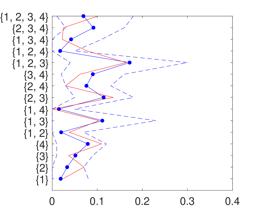
(a) $n=100$

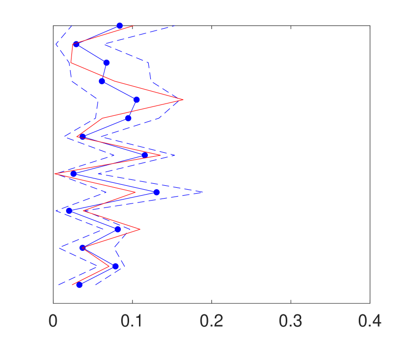
(b) $n=300$

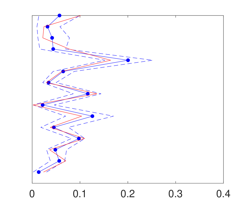
(c) $n=500$

Figure 1: The true distribution over consideration sets (solid, red), posterior mean (solid with dots, blue), 95% equal-tailed credible interval (dashed, blue). The results are based on the simulated data with $J=4$, $T=3$, and $n\in\{100,300,500\}$.

The vertical axis represents consideration sets and the horizontal axis shows the posterior distributions (solid with dots, blue) with the true distribution (solid, red), that is $\bm{\pi}^{*}$. The dashed lines (blue) represent the 95% credible intervals. As $n$ increases, the difference between the posterior and true distributions decreases.

Table 2: Estimation results from the simulation study with $J=4$

	$\delta_{1}$		$\delta_{2}$		$\delta_{3}$		$\beta$		$D^{1/2}$
$n=100$	0.49	(0.503)	0.36	(0.530)	0.02	(0.443)	0.47	(0.075)	1.30	(0.192)
$n=300$	0.20	(0.326)	0.19	(0.321)	0.19	(0.315)	0.04	(0.130)	0.19	(0.202)
$n=500$	0.08	(0.254)	0.21	(0.273)	0.09	(0.262)	0.07	(0.108)	0.16	(0.170)

• Estimation results for the fixed-effect parameters $\delta_{j}$’s and $\beta$ as well as the standard deviation $D^{1/2}$ of the random-effects. The absolute value of the difference between the posterior mean and the data-generating value is shown together with the posterior standard deviation (in parenthesis). The results are based on the simulated data with $J=4$.

Table 2 shows the estimation results regarding the parameters $(\delta_{1},\delta_{2},\delta_{3},\beta,D)$. Although this is not a repeated experiment, the discrepancy between the posterior mean and the data-generating value as well as the posterior standard deviation generally decrease for all the parameters as $n$ increases.

6 Application

6.1 Data Description

We obtained the household purchase panel and store data on the cold cereal category from Information Resources Inc. (IRI, Bronnenberg et al., 2008). The sample consists of household shopping trips in Eau Claire and Pittsfield during the first 14 weeks of 2007. We use the first 12 weeks for estimation and the last two weeks for out-of-sample prediction. The households that bought less than 3 units of cold cereal during the sample period are removed from the sample. When households made multiple products at one shopping trip, we treat them as separate purchases. This leaves us with $J=68$ brands and $n=428$ households in the sample. Note that with $J=68$, it is computationally impossible to work with all the $J^{*}=2^{J}-1>10^{19}$ probabilities of consideration sets as in Chiang et al. (1998).

For each shopping trip in the sample, we observe the household identifier, week, store, and brand purchased. Combining with household purchase history and store data corresponding to the sample period, we obtain the following information for each purchase occasion: the price, display, and feature for the brands at the week/store of the purchase, and the brands purchased. The UPC level price, display and feature advertising are aggregated into brand level for each store/week. Let $i\in\{1,\ldots,428\}$ and $t\in\{1,\ldots,T_{i}\}$ index household and purchase occasion, respectively. The mean of $T_{i}$ is 6.9 while the minimum and maximum are 3 and 32, respectively. The price $P_{ijt}$ of brand $j\in\{1,\ldots,J\}$ is a sale-weighted price index constructed from UPC level prices for the purchase occasion $t\in\{1,\ldots,T_{i}\}$ for household $i$. Also, display $D_{ijt}$ and feature $F_{ijt}$ are indicator variables that equals to 1 if any UPC within the brand is on display/featured. The Supplementary Material contains more information on data description.

The full specification is the following random-effects logit model conditional on consideration sets $\{\mathcal{C}_{i}\}$:

$$V_{ijt}=\delta_{j}+\bm{x}_{ijt}^{\prime}(\bm{\beta}+\bm{b}_{i}),$$

where $\delta_{j}$ denotes the brand-specific fixed-effect for $j$, $\bm{x}_{ijt}=[P_{ijt},D_{ijt},F_{ijt}]^{\prime}$ is a 3-dimensional vector containing information for brand $j$ at purchase occasion $t$ for $i$, $\delta_{j}$ is the brand-specific fixed-effect with $\delta_{J}=0$ for normalization, $\bm{\beta}$ is the vector of common fixed-effects, and $\bm{b}_{i}$ is the vector of random-effects that follows iid $N_{3}(\bm{0},\bm{D})$. Hence, in the full specification, we estimate $\{\bm{\delta},\bm{\beta},\{\bm{b}_{i}\},\bm{D}\}$ in the response model, which amounts to $(J-1+3+3n+6)=1360$ parameters/unknowns. In addition, we need to estimate the $Jn=29104$ unknown elements in $\{\bm{C}_{i}\}$ that represent the consideration sets, where the support of the distribution of each of the $J$-dimensional vector is exponentially large ($J^{*}=2^{J}-1>10^{19}$) in principle, but made tractable by the proposed approach.

We set the hyper prior parameters as follows: a sparsity-supporting prior for the attention probabilities $q_{hj}\sim\text{Beta}(\underline{a}_{q_{j}},\underline{b}_{q_{j}})$, independently over $j=1,\ldots,J$ for $h=1,\ldots,\infty$, with $(\underline{a}_{q_{j}},\underline{b}_{q_{j}})=(s\cdot r,s\cdot(1-r))$, $r=\frac{r_{0}}{J}$ with $s=5$ and $r_{0}=30$, which implies that the prior mean of $q_{hj}$ is about 0.44. For the DP concentration parameter, $\alpha\sim\text{Gamma}(2,4)$. The priors for $\bm{\delta}$ and $\bm{\beta}$ are independent normal distributions with zero mean and variance $3$. The prior for $\bm{D}$ is an inverse-Wishart distribution with hyper-parameters $(\underline{v},\underline{\bm{R}})=(9,(1/9)I)$.

We fit four variants of the multinomial logit (MNL) models to the cereal data set, depending on whether we include random-effects and/or consideration set heterogeneity (that is, incorporating and estimating latent consideration sets) as summarized in Table 3.

Model	MNL	MNL_R	MNL_C	MNL_RC
Random-effects	No	Yes	No	Yes
Consideration set heterogeneity	No	No	Yes	Yes

Table 3: The four variants of the multinomial logit (MNL) models

Each of the special cases can be estimated according to the simulation method developed in Section 4 by suppressing the component that is absent from the full hierarchical model.

6.2 Empirical Results

Table 4: Estimation results

	MNL		MNL_R		MNL_C		MNL_RC
Model covariate	mean	s.d.	mean	s.d.	mean	s.d.	mean	s.d.
common fixed-effects
Price	-0.2090*	0.0265	-0.2242*	0.0592	-0.2423*	0.0380	-0.2614*	0.0590
Display	1.1699*	0.0223	1.1807*	0.0811	1.2612*	0.0347	1.3953*	0.0889
Feature	0.0675*	0.0272	-0.0776	0.0727	-0.0101	0.0424	-0.0047	0.0807
s.d. of random-effects
$D^{1/2}_{11}$ (Price)	——	——	0.9810	0.0709	——	——	0.6044	0.1693
$D^{1/2}_{22}$ (Display)	——	——	1.5009	0.1065	——	——	1.3354	0.1253
$D^{1/2}_{33}$ (Feature)	——	——	1.1810	0.1022	——	——	0.6032	0.3144
brand-specific fixed-effects
Num. of ‘significant’ params	49		50		18		13
computational time
Min. per 1,000 MCMC iterations	6.7		11.1		12.9		17.6

• The first panel shows posterior means and standard deviations of the common fixed-effects $\bm{\beta}$. Stars indicate that the corresponding 95% credible interval does not include 0. The second panel shows the estimation results for the square root of the diagonal elements of $\bm{D}$. The third panel shows the number of brand-specific fixed effects whose 95% posterior credible intervals do not include 0. The last panel shows computational time (minutes) on a desktop with a 4.9GHz processor and 64GB RAM. The results are based on 10,000 posterior draws.

We summarize our empirical findings in Table 4. Comparisons of the estimated parameters in the response model across the four approaches reveal similar findings as in the previous literature that dealt with data sets with smaller $J$. See the Supplementary Material for an in-depth discussion on these points. In the following, we focus on the computational time, estimated parameters in the mixture model, and predictive performance.

6.2.1 Computational time

We estimated each of the four models and obtain 10,000 MCMC draws on a desktop with a 4.9GHz processor and 64GB RAM. The last panel of Table 4 shows the computational time in minutes per MCMC 1,000 draws. Compared to the standard logit model, the extra burden of estimating latent consideration sets according to our proposed approach is reasonable. For instance, the increase in the computational time when consideration sets are estimated in addition to random effects is roughly speaking 55% (11.1 mins for MNL_R and 17.6 mins for MNL_RC).

6.2.2 Estimated parameters in the mixture model

We investigate the clustering of subjects according to their consideration sets. The posterior mode of the number of the non-empty clusters under the full-specification (MNL_RC) is 7. The Supplementary Material shows the estimation results regarding the number of mixture clusters and the DP concentration parameter $\alpha$.

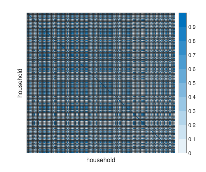
Figure 2: The 428 $\times$ 428 similarity matrix of households.

To understand how households are clustered, we computed the similarity matrix shown in Figure 2. The each entry of the matrix shows the posterior probability that a given household at a particular row $i$ is in the same cluster as another household at a specific column $i^{\prime}$, which is computed as the posterior mean of the event $\{S_{i}=S_{i^{\prime}}\}$, ranging from zero (light blue) to one (dark blue). An examination of how households are clustered reveals interesting points. Let us take household 63 as an example whose actual choices consist of $\{32,39,59\}$. Define an estimator $\hat{\mathcal{C}}_{i}$ of the consideration set for household $i$ as the set of brands $j$ whose posterior probability of $C_{ij}=1$ is greater than 0.5. This results in the estimated set $\hat{\mathcal{C}}_{63}=\{2,10,32,39,40,44,59\}$.

Table 5: Households clustered with $i\in\{63,414\}$.

• Similarity is defined as the posterior mean of $1\{S_{i^{\prime}}=S_{i}\}$, which corresponds to the ith row (equivalently ith column) of the similarity matrix in Figure 2. The estimated consideration set $\hat{\mathcal{C}}_{i}$ is defined as the set of brands $j$ whose posterior median probability of $\{C_{ij}=1\}$ is greater than 0.5. The result is from the MNL_PC model.

$i^{\prime}$	Similarity	Chosen brands	Estimated $\hat{\mathcal{C}}_{i^{\prime}}$
Household $i=63$
$i^{\prime}=63$	1.00	$\{32,39,59\}$	$\{2,10,32,39,40,44,59\}$
$i^{\prime}=258$	0.76	$\{30,31,32,38,39,40,42,44\}$	$\{1,2,30,31,32,38,39,40,42,44\}$
$i^{\prime}=152$	0.75	$\{1,3,8,20,32,39,42,59\}$	$\{1,3,8,20,32,36,39,42,52,59\}$
$i^{\prime}=229$	0.74	$\{10,13,30,36,39,40,67\}$	$\{2,3,10,12,13,30,36,39,40,52,67\}$
Household $i=414$
$i^{\prime}=414$	1.00	$\{2,3,12,30,32,36,39\}$	$\{2,3,12,30,32,36,39,52\}$
$i^{\prime}=380$	0.99	$\{2,3,12,20,36,39\}$	$\{2,3,10,12,20,36,39,40,52\}$
$i^{\prime}=416$	0.98	$\{2,4,12,16,23,30,32,36,40,54\}$	$\{2,3,4,12,16,23,30,32,36,39,40,52,54\}$
$i^{\prime}=156$	0.98	$\{2,12,24,30,36,39\}$	$\{2,3,12,24,30,32,36,39,52\}$

The upper panel of Table 5 lists the three households with the highest posterior similarity to subject $63$. There are several observations. First, we notice that the actual choices of the households tend to overlap within a cluster. For example, the four subjects chose brands 32 and/or 39. Second, the estimated consideration sets $\hat{\mathcal{C}}_{i^{\prime}}$ are similar between households in a cluster. For example, household 63 did not choose brands 40 and 44, but household 258 did, and they are in $\hat{\mathcal{C}}_{63}$. Third, the stronger the overlap in the actual choices of the households, the higher the chance of being in the same cluster. See the lower panel of Table 5 for the results for household 414. The four households purchased brands 2, 12, and 36, and show high similarity scores ($\geq 0.98$). In this way, our algorithm discovers the probabilistic grouping patterns in the choice data.

6.2.3 Predictive performance

We compute the posterior distribution conditional on data on the responses and covariates $(\bm{y},\bm{\omega})$ from the first 12 weeks of the sample period. To examine the predictive performance of the model, we reserve the sample from the following 2 weeks as test data for making predictions. Denote the set of subjects who made purchases during the out-of-sample period by $\mathcal{O}\subset\{1,\ldots,n\}$. There are 173 households in $\mathcal{O}$. For each household in this set, we predict $\bm{Y}^{f}_{i}=\{Y_{iT_{i}+s}:s=1,\ldots,h_{i}\}$, given the newly available covariates $\bm{\omega}^{f}_{i}=\{\bm{\omega}_{iT_{i}+s}:s=1,\ldots,h_{i}\}$, where $h_{i}$ denotes the forecast horizon for the subject $i$. Let $\bm{y}^{f}_{i}=\{y_{iT_{i}+s}:s=1,\ldots,h_{i}\}$ be the actual set of responses for the subject $i\in\mathcal{O}$. The predictive likelihood for this subject is

$$p(\bm{y}^{f}_{i}|\bm{y},\bm{\omega},\bm{\omega}^{f}_{i}) =\int\prod_{s=1}^{h_{i}}\Pr(Y_{iT_{i}+s}=y_{iT_{i}+s}|\bm{\delta},\bm{\beta},\bm{b}_{i},\bm{\omega}_{iT_{i}+s},\mathcal{C}_{i})d\pi(\bm{\delta},\bm{\beta},\{\bm{b}_{i}\},\{\mathcal{C}_{i}\}|\bm{y},\bm{\omega})$$

$$\approx\frac{1}{G}\sum_{g=1}^{G}\prod_{s=1}^{h_{i}}\Pr(Y_{iT_{i}+s}=y_{iT_{i}+s}|\bm{\delta}^{(g)},\bm{\beta}^{(g)},\bm{b}_{i}^{(g)},\bm{\omega}_{iT_{i}+s},\mathcal{C}_{i}^{(g)}),$$ (13)

where the response probability conditional on a consideration set is given in (1).

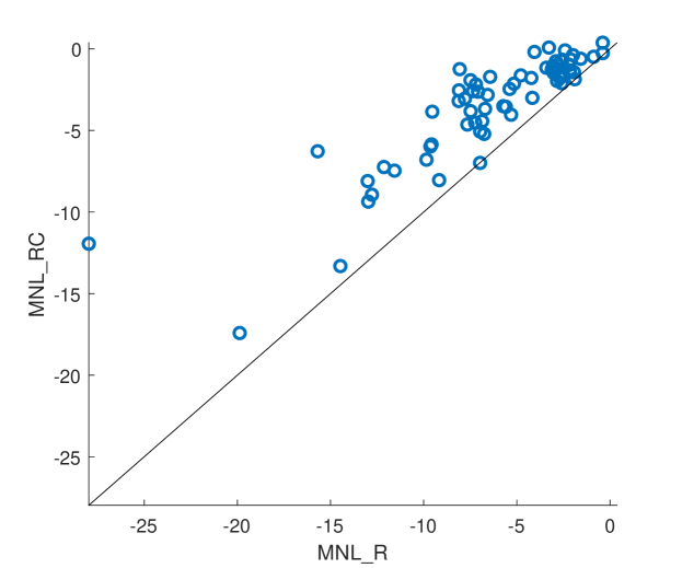
Figure 3: Log-predictive likelihood (circles) for the 173 households that made purchases in the out-of-sample period based on MNL_R (horizontal) and MNL_RC (vertical) with the 45-degree line (solid).

Figure 3 gives the log-predictive likelihood for each subject under the (MNL_R) and (MNL_RC) models. This figure shows that including the heterogeneity of the consideration set improves the predictions. Importantly, this is perhaps the first such predictive comparison in the large $J$ case, made possible by the scalable procedure developed in this paper.

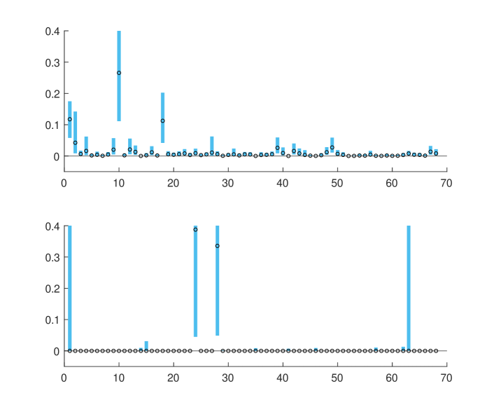
Figure 4: Estimated predictive response probabilities $\Pr(Y_{i,T_{i}+1}=j)$ for $i=164$. 90% credible intervals (bars) and medians (circles). The horizontal axis represents the brands $j\in\{1,\ldots,68\}$. The actual out-of-sample purchase was brand 24.

To investigate why MNL_RC outperforms MNL_R in prediction, we compare the estimated response probabilities between the two models. For each $i\in\mathcal{O}$, we can compute the marginal posterior of $\Pr(Y_{iT_{i}+s}=j)$, for each alternative $j$ and forecasting horizon $s=1,\ldots,h_{i}$. Figure 4 presents the estimated response probabilities for the household $i=164$ in the first out-of-sample period, $s=1.$ This household repeatedly purchased brands 24 and 28 in the estimation sample: $\{24,24,28,28,24,24,24,28,28,28,28\}$, in the order of the purchases. In the out-of-sample week, the household purchased brand 24. The figure shows the 90% credible intervals (vertical bars) as well as the median of the estimated response probabilities (circles). Clearly, the estimated response probabilities are much sparser for MNL_RC than MNL_R. The traditional MNL approach necessarily implies a positive probability for every alternative. In contrast, the consideration set model allows many alternatives to actually receive zero predictive probabilities. Thus, incorporating consideration set heterogeneity can improve predictive performance when the time-invariant consideration set assumption is appropriate, which seems to be the case in this data set.

In this empirical section, we demonstrated that the added computational effort of estimating latent consideration sets under the proposed approach is reasonable, while there is a significant improvement in predictive performance, compared to the standard (random-effects) logit models. The estimation results for the parameters in the response model seem to be generally consistent with previous findings in the literature (an in-depth discussion can be found in the Supplementary Material).

7 Conclusion

In this article, we proposed a scalable modeling and estimation scheme for multinomial response models with uncertain consideration sets. The approach relies on a factor decomposition technique to flexibly model the distribution over the latent consideration sets. We showed that our approach can be applied to situations beyond the reach of existing methods. For example, we considered a simulated data example with $J=100$ categories and a real data example with $J=68$ categories. In the latter case, we also demonstrated that the new model leads to improved out-of-sample predictions relative to the standard multionomial logit model, a comparison made possible by the scalable approach developed in this paper.

As described in the introduction, the latent consideration set models have been applied in many fields such as economics, marketing, psychology, and transportation science, but its application has been limited to data sets with small numbers of alternatives. The methodology proposed in this paper thus provides new opportunities for empirical researchers in multiple disciplines to consider and estimate large-dimensional multinomial logit models with latent consideration sets.

Appendix A Proof of Theorem 1

Proof of Theorem 1.

The proof is by an application of Schwartz’s theorem (see Norets and Pelenis (2014) for a general discussion on applying the theorem for conditional density estimation) and the proof strategy is based on Norets and Shimizu (2022). Our aim is to show that $\Pi((\bm{\theta},\bm{\pi})\in KL_{\varepsilon}(\bm{p}^{*}))>0$; that is, the prior puts positive probability on the KL neighborhood of the true response distribution $\bm{p}^{*}$. Lemma 2 establishes that the KL-divergence around $\bm{p}^{*}$ is continuous. The lemma combined with a prior that places positive mass on open neighborhoods (condition iii) implies that $\Pi(KL_{\varepsilon}(\bm{p}^{*}))>0$. ∎

Lemma 2.

[Continuity of the KL divergence around $p^{*}$] Suppose that conditions (i) and (ii) of Theorem 2 hold. Then $\forall\varepsilon>0$, $\exists K\in\mathbb{Z}^{+}$ and open neighborhoods $\Theta$ of $\theta^{*}$ and $\Phi^{K}$ of $\bm{\pi}^{*}$ such that for any $\bm{\theta}\in\Theta$ and $\bm{\phi}_{1K}\in\Phi^{K}$,

$$\int\sum_{j=1}^{J}\log\left(\frac{p_{\bm{\theta}^{*},\bm{\pi}^{*}}(j|\bm{w})}{p(j|\bm{w};\bm{\theta},K,\bm{\phi}_{1K})}\right)p_{\bm{\theta}^{*},\bm{\pi}^{*}}(j|\bm{w})g^{*}(\bm{w})d\bm{w}<\varepsilon.$$

Proof.

By Theorem 1 of Dunson and Xing (2009), we can find a finite mixture of independent consideration models that exactly matches the true distribution of consideration sets; i.e. $\exists(K,\tilde{\bm{\phi}}_{1K})$ such that $\pi^{*}_{c}=\sum_{h=1}^{K}\tilde{\omega}_{h}\prod_{j\in c}\tilde{q}_{hj}\prod_{j\notin c}(1-\tilde{q}_{hj})$ for each $c\in\mathcal{C}$. Hence

$$\int\sum_{j=1}^{J}\log\left(\frac{p_{\bm{\theta}^{*},\bm{\pi}^{*}}(j|\bm{w})}{p(j|\bm{w};\bm{\theta},K,\bm{\phi}_{1K})}\right)p_{\bm{\theta}^{*},\bm{\pi}^{*}}(j|\bm{w})g^{*}(\bm{w})d\bm{w}$$

$$=\int\sum_{j=1}^{J}\left\{\log\left(\frac{p_{\bm{\theta}^{*},\bm{\pi}^{*}}(j|\bm{w})}{p(j|\bm{w};\bm{\theta}^{*},K,\tilde{\bm{\phi}}_{1K})}\right)+\log\left(\frac{p(j|\bm{w};\bm{\theta}^{*},K,\tilde{\bm{\phi}}_{1K})}{p(j|\bm{w};\bm{\theta},K,\bm{\phi}_{1K})}\right)\right\}p_{\bm{\theta}^{*},\bm{\pi}^{*}}(j|\bm{w})g^{*}(\bm{w})d\bm{w},$$

where the first term in the brackets is zero. In the Supplementary Material, we prove that the response probability is continuous in $\bm{\phi}_{1K}$ (Lemma SB1) and it is continuous also in $\bm{\theta}$ (Lemma SB2). Let $(\bm{\theta}^{m},\bm{\phi}_{1K}^{m})$ be a sequence of parameter values converging to $(\bm{\theta}^{*},\tilde{\bm{\phi}}_{1K})$. Then

$$\lim_{m\to\infty}\log\left(\frac{p(j|\bm{w};\bm{\theta}^{*},K,\tilde{\bm{\phi}}_{1K})}{p(j|\bm{w};\bm{\theta}^{m},K,\bm{\phi}^{m}_{1K})}\right)=0.$$

The result will follow from the dominated convergence theorem if there is an integrable (with respect to $p_{\bm{\theta}^{*},\bm{\pi}^{*}}(j|\bm{w})g^{*}(\bm{w})$) upper bound of $|\log p(j|\bm{w};\bm{\theta}^{m},K,\bm{\phi}_{1K}^{m})|$. Note that

$$p(j|\bm{w};\bm{\theta}^{m},K,\bm{\phi}_{1K}^{m})=\sum_{c\in\mathcal{C}}\pi(c|K,\bm{\phi}^{m}_{1K})\Pr(j|\bm{\theta}^{m},\bm{w},c)$$

$$\geq\pi(c_{j}|K,\bm{\phi}^{m}_{1K})\Pr(j|\bm{\theta}^{m},\bm{w},c_{j})=\left\{\sum_{h=1}^{K}\omega_{h}^{m}\prod_{\ell\in c_{j}}q^{m}_{h\ell}\prod_{\ell\notin c_{j}}(1-q^{m}_{h\ell})\right\}\Pr(j|\bm{\theta}^{m},\bm{w},c_{j}),$$

where by the assumption (ii), $c_{j}\in\mathcal{C}$ contains $j$, $\pi^{*}_{c_{j}}>0$, and $\Pr(j|\bm{\theta}^{*},\bm{w},c_{j})>0$ for all $\bm{w}\in\mathcal{W}$. First, since $\bm{\phi}^{m}_{1K}\to\tilde{\bm{\phi}}_{1K}$ and $\pi^{*}_{c_{j}}=\sum_{h=1}^{K}\tilde{\omega}_{h}\prod_{\ell\in c_{j}}\tilde{q}_{h\ell}\prod_{\ell\notin c_{j}}(1-\tilde{q}_{h\ell})>0$, the term in the curly brackets is bounded below by some $\ell_{1}(j,\bm{w})>0$ for sufficiently large $m$. Second, since $\bm{\theta}^{m}\to\bm{\theta}^{*}$ and $\Pr(j|\bm{\theta}^{*},\bm{w},c_{j})>0$, $\Pr(j|\bm{\theta}^{m},\bm{w},c_{j})$ is bounded below by some $\ell_{2}(j,\bm{w})>0$ for sufficiently large $m$. Lastly, $1\geq p(j|\bm{w};\bm{\theta}^{m},K,\bm{\phi}_{1K}^{m})\geq\inf_{\bm{w}\in\mathcal{W}}\min_{j\in\mathcal{J}}\ell_{1}(j,\bm{w})\ell_{2}(j,\bm{w})>0,$ for all $(j,\bm{w})\in\mathcal{J}\times\mathcal{W}.$ ∎

Acknowledgement

We benefited from useful comments from Paola Manzini, Francesca Molinari, Nail Kashaev, Alessandro Iaria, Ao Wang, Elena Manresa, Dimitris Korobilis, Martin Weidner, Laura Liu, Asim Ansari, Andriy Norets, Toru Kitagawa, Frank Schorfheide, Zhentong Lu, and the audience at the 2023 NBER-NSF Seminar in Bayesian Econometrics and Statistics (SBIES) at the Federal Reserve Bank of Philadelphia as well as the 2023 INFORMS Annual Meeting in Phoenix.

SUPPLEMENTARY MATERIAL

Section SB presents the conditional posterior distributions of the parameters other than the consideration sets. Section SC provides the proofs. Section SD illustrates the impact of the prior choice for the attention probabilities on the prior on the distribution of consideration sets. Section SE presents a simulation study under a large number of alternatives, $J=100.$ Section SF provides additional results from the empirical application.

Appendix SB Conditional posterior distributions

Our MCMC algorithm proceeds by cycling through various conditional distributions, where these distributions are conditioned on the most recent values of the remaining unknowns. Specifically, given the current draw at the $g$th iteration $\{u_{i}^{(g)}\},\{V_{h}^{(g)}\},\{\bm{q}_{h}^{(g)}\},\{S_{i}^{(g)}\},$ $\alpha^{(g)}$, $\big{\{}\bm{C}_{i}^{(g)}\big{\}},\bm{\delta}^{(g)}$, $\bm{\beta}^{(g)},\big{\{}\bm{b}_{i}^{(g)}\big{\}}$, and $\bm{D}^{(g)}$, the next draw in the sequence is obtained by simulating

$$\bm{\beta}^{(g+1)} \text{ from }\bm{\beta}\big{|}\big{\{}y_{it}\big{\}},\big{\{}\bm{C}_{i}^{(g)}\big{\}},\bm{\delta}^{(g)},\big{\{}\bm{b}_{i}^{(g)}\big{\}},$$

$$\big{\{}\bm{b}_{i}^{(g+1)}\big{\}} \text{ from }\big{\{}\bm{b}_{i}\big{\}}\big{|}\big{\{}y_{it}\big{\}},\big{\{}\bm{C}_{i}^{(g)}\big{\}},\bm{\delta}^{(g)},\bm{\beta}^{(g+1)},\bm{D}^{(g)},$$

$$\bm{D}^{(g+1)} \text{ from }\bm{D}\big{|}\big{\{}\bm{b}_{i}^{(g+1)}\big{\}},$$

$$\bm{\delta}^{(g+1)} \text{ from }\bm{\delta}\big{|}\big{\{}y_{it}\big{\}},\big{\{}\bm{C}_{i}^{(g)}\big{\}},\bm{\beta}^{(g+1)},\big{\{}\bm{b}_{i}^{(g+1)}\big{\}},$$

$$\big{\{}\bm{C}_{i}^{(g+1)}\big{\}} \text{ from }\big{\{}\bm{C}_{i}\big{\}}\big{|}\big{\{}y_{it}\big{\}},\bm{\delta}^{(g+1)},\bm{\beta}^{(g+1)},\big{\{}\bm{b}_{i}^{(g+1)}\big{\}},\{\bm{q}_{h}^{(g)}\},\{S_{i}^{(g)}\},$$

$$\{V_{h}^{(g+1)}\} \text{ from }\{V_{h}\}\big{|}\{S_{i}^{(g)}\},\alpha^{(g)},$$

$$\{\bm{q}_{h}^{(g+1)}\} \text{ from }\{\bm{q}_{h}\}\big{|}\big{\{}\bm{C}_{i}^{(g+1)}\big{\}},\{S_{i}^{(g)}\},$$

$$\{u_{i}^{(g+1)}\} \text{ from }\{u_{i}\}\big{|}\{S_{i}^{(g)}\},\{V_{h}^{(g+1)}\},$$

$$\{S_{i}^{(g+1)}\} \text{ from }\{S_{i}\}\big{|}\{u_{i}^{(g+1)}\},\{\bm{q}_{h}^{(g+1)}\},\{V_{h}^{(g+1)}\},\big{\{}\bm{C}_{i}^{(g+1)}\big{\}},$$

$$\alpha^{(g+1)} \text{ from }\alpha\big{|}\{V_{h}^{(g+1)}\},\{S_{i}^{(g+1)}\}.$$

Repeating this procedure $G$ times (beyond a suitable burn-in) produces a sample from the posterior distribution.

The main paper illustrates how the consideration sets are simulated. In this section, we show the conditional posterior distributions of the remaining parameters.

For the mixture model, recall we have

$$p(\bm{C},\bm{S},\bm{Q},\bm{V},\bm{u},\alpha)\propto\left[\prod_{i=1}^{n}p\big{(}\bm{C}_{i}|\bm{q}_{S_{i}}\big{)}I(u_{i}\leq\omega_{S_{i}})\right]\cdot\left[\prod_{h=1}^{\infty}p\big{(}V_{h}|\alpha\big{)}p(\bm{q}_{h}|\underline{\bm{\phi}}_{q}\big{)}\right]\cdot\pi(\alpha).$$ (SB.1)

Let $K^{*}=\min\{h:\sum_{\ell=1}^{h}\omega_{h}>1-u^{*}\}$, where $u^{*}=\min(u_{1},\ldots,u_{n}).$ Define $n_{h}=\sum_{i=1}^{n}I(S_{i}=h)$. Let the dot $\bullet$ denote all other parameters and the data.

SB.1 Simulation of $q_{h}$

From (SB.1), we have that

$$p(\bm{q}_{h}|\bullet)\propto p(\bm{q}_{h}|\underline{\bm{\phi}}_{q}\big{)}\cdot\prod_{i:S_{i}=h}\prod_{j=1}^{J}q_{hj}^{C_{ij}}\left(1-q_{hj}\right)^{1-C_{ij}},$$

where $p(\bm{q}_{h}|\underline{\bm{\phi}}_{q}\big{)}$ is the product of densities for Beta distributions $Beta(\underline{a}_{q_{j}},\underline{b}_{q_{j}})$, independently over $j=1,\ldots,J$. Then

$$q_{hj}|\bullet\sim\text{Beta}\left(\underline{a}_{q_{j}}+\sum_{i:S_{i}=h}C_{ij},\underline{b}_{q_{j}}+\sum_{i:S_{i}=h}(1-C_{ij})\right),$$

independently over $j=1,\ldots,J$ for $h=1,2,\ldots,K^{*}$. If component $h\leq K^{*}$ does not contain any observations, then the corresponding $\bm{q}_{h}$ is drawn from the prior.

SB.2 Simulation of $V_{h}$

Integrating $\bm{u}$ out from (SB.1), we have

$$p(\bm{V},\bm{C},\bm{S},\bm{Q},\bm{u},\alpha)\propto\left[\prod_{i=1}^{n}p\big{(}\bm{C}_{i}|\bm{q}_{S_{i}}\big{)}\omega_{S_{i}}\right]\cdot\left[\prod_{h=1}^{\infty}p\big{(}V_{h}|\alpha\big{)}p(\bm{q}_{h}|\underline{\bm{\phi}}_{q}\big{)}\right]\cdot\pi(\alpha)$$

From the form of the joint distribution above, the conditional distribution of $\bm{V}$ is independent and the marginal conditional distributions are

$$V_{h}|\bullet\sim\text{Beta}\left(1+n_{h},\alpha+\sum_{\ell>h}n_{\ell}\right),$$

for $h=1,2,\ldots,K^{*}$. If component $h\leq K^{*}$ is empty, then the corresponding $V_{h}$ is drawn from the prior.

SB.3 Simulation of $u_{i}$

From (SB.1), it is easy to see that

$$u_{i}|\bullet\overset{ind}{\sim}\mathcal{U}[0,\omega_{S_{i}}],\quad i=1,\ldots,n.$$

SB.4 Simulation of $S_{i}$

From (SB.1), we can see that for $h=1,2,\ldots,K^{*}$,

$$Pr\left(S_{i}=h|\bm{C},\bm{u},\bm{V},\bm{Q}\right)=\frac{I\left(u_{i}\leq\omega_{h}\right)\prod_{j=1}^{J}q_{hj}^{C_{ij}}\left(1-q_{hj}\right)^{1-C_{ij}}}{\sum_{\ell}I\left(u_{i}\leq\omega_{\ell}\right)\prod_{j=1}^{J}q_{\ell j}^{C_{ij}}\left(1-q_{\ell j}\right)^{1-C_{ij}}}.$$

Note that $Pr(S_{i}=h|\bullet)=0$ for $h>K^{*}$.

SB.5 Simulation of $\alpha$

The conditional posterior of $\alpha$ is

$$p(\alpha|\bullet)\propto p(\bm{S}|\alpha)\pi(\alpha).$$

Following Escobar and West (1995), this distribution is sampled by first generating $\eta$ conditional on $\alpha$ from the Beta distribution

$$\eta|\alpha,\bm{S}\sim\text{Beta}(\alpha+1,n),$$

and then sampling $\alpha$ conditional on $\eta$ from the Gamma mixture

$$p(\alpha|\eta,\bm{S}) =\frac{\underline{a}_{\alpha}+G-1}{\underline{a}_{\alpha}+G-1+n(\underline{b}_{\alpha}-\log(\eta))}\text{Gamma}(\underline{a}_{\alpha}+G,\underline{b}_{\alpha}-\log(\eta))$$

$$+\frac{n(\underline{b}_{\alpha}-\log(\eta))}{\underline{a}_{\alpha}+G-1+n(\underline{b}_{\alpha}-\log(\eta))}\text{Gamma}(\underline{a}_{\alpha}+G-1,\underline{b}_{\alpha}-\log(\eta)),$$

where $G$ is the total number of existing clusters.

SB.6 Simulation of $\beta$

From Bayes theorem,

$$\pi(\bm{\beta}|\bullet)\propto\pi(\bm{\beta})\cdot\prod_{i=1}^{n}\prod_{t=1}^{T_{i}}\Pr(Y_{it}=y_{it}|\bm{\delta},\bm{\beta},\bm{b}_{i},\bm{\omega}_{it},\mathcal{C}_{i}),$$

where $\Pr(Y_{it}=y_{it}|\bm{\delta},\bm{\beta},\bm{b}_{i},\bm{\omega}_{it},\mathcal{C}_{i})=\frac{\exp\left(V_{iy_{it}t}\right)}{\sum_{\ell\in\mathcal{C}_{i}}\exp\left(V_{i\ell t}\right)}$ and $V_{ijt}=\delta_{j}+\bm{x}_{ijt}^{\prime}\bm{\beta}+\bm{z}_{ijt}^{\prime}\bm{b}_{i}$.

We use a tailored Metropolis–Hastings (M-H) algorithm to sample $\bm{\beta}$ (Chib and Greenberg, 1995). Define the conditional log-likelihood of $\bm{\beta}$ given $\bm{\delta}$, $\{\bm{b}_{i}\}$, and $\{\bm{C}_{i}\}$: $\log L(\bm{\beta}|\bullet)=\sum_{i=1}^{n}\sum_{t=1}^{T_{i}}\log\Pr(Y_{it}=y_{it}|\bm{\delta},\bm{\beta},\bm{b}_{i},\mathcal{C}_{i}).$ At iteration $g$, let $\bm{\beta}^{(g)}$ be the value of $\bm{\beta}$. A candidate value is drawn as

$$\tilde{\bm{\beta}}\sim N_{d_{x}}\left(\hat{\bm{\beta}},\hat{\bm{V}}_{\beta}\right),$$

where

$$\hat{\bm{\beta}}=\arg\max_{\bm{\beta}}\log L(\bm{\beta}|\bullet)\pi(\bm{\beta}),\quad\ \hat{\bm{V}}_{\beta}^{-1}=-\frac{\partial^{2}}{\partial\bm{\beta}\partial\bm{\beta}^{\prime}}\log L(\bm{\beta}|\bullet)\pi(\bm{\beta})\bigg{|}_{\bm{\beta}=\hat{\bm{\beta}}},$$

which is accepted with probability

$$\min\left\{\frac{\pi(\tilde{\bm{\beta}}|\bullet)\phi(\bm{\beta}^{(g)}|\hat{\bm{\beta}},\hat{\bm{V}}_{\beta})}{\pi(\bm{\beta}^{(g)}|\bullet)\phi(\tilde{\bm{\beta}}|\hat{\bm{\beta}},\hat{\bm{V}}_{\beta})},1\right\},$$

where $\phi(\ \ )$ denotes the density of normal distribution. The conditional posterior mode $\hat{\bm{\beta}}$ is computed using the Newton-Raphson method. The likelihood is known to be concave with respect to $\bm{\beta}$ under the Gumbel error distribution, so the convergence to $\hat{\bm{\beta}}$ is fast and only requires a few iterations in many cases. In the empirical application, we multiply the variance of the proposal distribution by $10^{-2}$ in order to achieve desirable acceptance rates.

SB.7 Simulation of $b_{i}$

The full conditional of $\bm{b}_{i}$ (for each $i$) is proportional to

$$\pi(\bm{b}_{i}|\bullet)\propto\phi(\bm{b}_{i}|\bm{0},\bm{D})\cdot\prod_{t=1}^{T_{i}}\Pr(Y_{it}=y_{it}|\bm{\delta},\bm{\beta},\bm{b}_{i},\bm{\omega}_{it},\mathcal{C}_{i}).$$

We use a symmetric random-walk M-H to draw from the conditional distribution. Define the conditional log-likelihood of $\bm{b}_{i}$ given $\bm{\delta}$, $\bm{\beta}$, and $\{\bm{C}_{i}\}$: $\log L(\bm{b}_{i}|\bullet)=\sum_{t=1}^{T_{i}}\log\Pr(Y_{it}=y_{it}|\bm{\delta},\bm{\beta},\bm{b}_{i},\bm{\omega}_{it},\mathcal{C}_{i}).$ At iteration $g$, let $\bm{b}_{i}^{(g)}$ be the value of $\bm{b}_{i}$. A candidate value is drawn as

$$\tilde{\bm{b}}_{i}\sim N_{d_{z}}\left(\bm{b}_{i}^{(g)},\bm{D}^{(g)}\right),$$

which is accepted with probability

$$\min\left\{\frac{\pi(\tilde{\bm{b}}_{i}|\bullet)}{\pi(\bm{b}_{i}^{(g)}|\bullet)},1\right\}.$$

The updating step for $b_{i}$ is independent over $i$, so it can be easily parallelized in a modern computer.

SB.8 Simulation of $D$

We simulate $\bm{D}$ by first simulating $\bm{D}^{-1}$ and then taking the inverse of the simulated draw. This is because it can be shown that

$$\bm{D}^{-1}|\bullet\sim\text{Wishart}\left(\underline{v}+n,\left[\underline{\bm{R}}^{-1}+\sum_{i=1}^{n}\bm{b}_{i}\bm{b}_{i}^{\prime}\right]^{-1}\right).$$

SB.9 Simulation of $\delta$

In princple, we could treat $\bm{\delta}$ as a part of $\bm{\beta}$ and sample from the conditional distribution altogether using a tailored M-H algorithm. However, the involved optimization step could be slow when $J$ is large, which is exactly our focus of the current paper. Hence, we sample $\bm{\delta}$ separately from $\bm{\beta}$. Specifically, we use a tailored Metropolis–Hastings (M-H) algorithm to sample $\delta_{k}$ for $k=1,\ldots,J-1,$ one after another.

From Bayes theorem,

$$\pi(\delta_{k}|\bm{\delta}_{\setminus k},\bm{\beta},\bm{b},\bm{\omega},\bm{C})\propto\pi(\delta_{k})\cdot\prod_{i=1}^{n}\prod_{t=1}^{T_{i}}\Pr(Y_{it}=y_{it}|\bm{\delta},\bm{\beta},\bm{b}_{i},\bm{\omega}_{it},\mathcal{C}_{i}),$$

where $\bm{\delta}_{\setminus k}$ denotes $\bm{\delta}$ except for the $k$th element. Define the conditional log-likelihood of $\delta_{k}$ given $\bm{\delta}_{\setminus k}$, $\bm{\beta}$, $\{\bm{b}_{i}\}$, and $\{\bm{C}_{i}\}$: $\log L(\delta_{k}|\bullet)=\sum_{i=1}^{n}\sum_{t=1}^{T_{i}}\log\Pr(Y_{it}=y_{it}|\bm{\delta},\bm{\beta},\bm{b}_{i},\bm{\omega}_{it},\mathcal{C}_{i}).$ At iteration $g$, let $\delta_{k}^{(g)}$ be the value of $\delta_{k}$. A candidate value is drawn as

$$\tilde{\delta}_{k}\sim N_{1}\left(\hat{\delta}_{k},\hat{\sigma}^{2}_{\delta_{k}}\right),$$

where

$$\hat{\delta}_{k}=\arg\max_{\delta_{k}}\log L(\delta_{k}|\bullet)\pi(\delta_{k}),\quad\ \hat{\sigma}^{-2}_{\delta_{k}}=-\frac{\partial^{2}}{\partial\delta_{k}^{2}}\log L(\delta_{k}|\bullet)\pi(\delta_{k})\bigg{|}_{\delta_{k}=\hat{\delta}_{k}},$$

which is accepted with probability

$$\min\left\{\frac{\pi(\tilde{\delta}_{k}|\bullet)\phi(\delta_{k}^{(g)}|\hat{\delta}_{k},\hat{\sigma}^{2}_{\delta_{k}})}{\pi(\delta_{k}^{(g)}|\bullet)\phi(\tilde{\delta}_{k}|\hat{\delta}_{k},\hat{\sigma}^{2}_{\delta_{k}})},1\right\}.$$

We randomize the order of updating $\delta_{k}$, $k=1,\ldots,J-1$.

Appendix SC Intermediate theoretical results and proofs

SC.1 Proof of the sparsity property of the proposed M-H step

Proposition 1 (Sparsity-inducing property).

Consider the M-H step described in Algorithm 1. Let $j$ be an alternative that is not observed to be chosen by the subject $i$. If the step proposes to exclude $j$ from the consideration set of $i$, it is accepted with probability 1.

Proof.

Let the consideration set for the $i$th subject at iteration $g$ be $\mathcal{C}_{i}^{(g)}$. Suppose that a category $j\in\mathcal{C}_{i}^{(g)}$ is proposed to be removed so that $\tilde{\mathcal{C}}_{i}=\mathcal{C}^{(g)}_{i}\setminus\{j\}$. The acceptance probability is

$$\min\left\{\frac{p\big{(}\bm{Y}_{i}=\bm{y}_{i}\big{|}\bm{\beta}^{(g)},\bm{b}_{i}^{(g)},\bm{\omega}_{i},\tilde{\mathcal{C}}_{i}\big{)}}{p\big{(}\bm{Y}_{i}=\bm{y}_{i}\big{|}\bm{\beta}^{(g)},\bm{b}_{i}^{(g)},\bm{\omega}_{i},\mathcal{C}^{(g)}_{i}\big{)}},1\right\}=\min\left\{\frac{\prod_{t}\sum_{\ell\in\mathcal{C}^{(g)}_{i}}\exp\left(V_{i\ell t}\right)}{\prod_{t}\sum_{\ell\in\tilde{\mathcal{C}}_{i}}\exp\left(V_{i\ell t}\right)},1\right\}=1,$$

where $V_{ijt}=\delta_{j}^{(g)}+\bm{x}_{ijt}^{\prime}\bm{\beta}^{(g)}+\bm{z}_{ijt}^{\prime}\bm{b}_{i}^{(g)}$, and the last equality is due to the fact that the ratio is larger than 1. Hence, $\tilde{\mathcal{C}}_{i}$ is accepted with probability 1. ∎

SC.2 Intermediate results in the proof of Theorem 2

The following two lemmas are used to prove Theorem 2 of the main paper. They state that the marginal response probability is continuous with respect to the mixture parameters as well as the parameters in the response model. Given $(K,\bm{\phi}_{1K})$, define the model induced probability for a consideration set $c\in\mathcal{C}$:

$$\pi(c|K,\bm{\phi}_{1K})=\sum_{h=1}^{K}\omega_{h}\prod_{j\in c}q_{hj}\prod_{j\notin c}(1-q_{hj})$$

and the model induced marginal response probability as

$$\Pr(j|\bm{w};\bm{\theta},K,\bm{\phi}_{1K})=\sum_{c\in\mathcal{C}}\pi(c|K,\bm{\phi}_{1K})Pr(j|\bm{\theta},\bm{w},c).$$

Lemma SC.1 (Continuity of response probabilities wrt mixture parameters).

Let $\bm{\theta}$ and $\bm{w}\in\mathcal{W}$. Then for each $j\in\mathcal{J}$, $\forall\varepsilon>0$ and $\bm{\phi}_{1K}^{(1)}$, $\exists\delta>0$ such that for any $\bm{\phi}_{1K}^{(2)}$ satisfying $\sum_{j=1}^{J}|q_{hj}^{(1)}-q_{hj}^{(2)}|<\delta$ and $|\omega_{h}^{(1)}-\omega_{h}^{(2)}|<\delta$, for $h=1,\ldots,K$, we have

$$\left|p(j|\bm{w};\bm{\theta},K,\bm{\phi}_{1K}^{(1)})-p(j|\bm{w};\bm{\theta},K,\bm{\phi}_{1K}^{(2)})\right|<\varepsilon.$$

Proof of Lemma SC.1.

We have

$$\left|p(j|\bm{w};\bm{\theta},K,\bm{\phi}_{1K}^{(1)})-p(j|\bm{w};\bm{\theta},K,\bm{\phi}_{1K}^{(2)})\right|\leq\sum_{c\in\mathcal{C}}\left|\pi(c|K,\bm{\phi}_{1K}^{(1)})-\pi(c|K,\bm{\phi}_{1K}^{(2)})\right|\Pr(j|\bm{\theta}^{(1)},\bm{w},c),$$

where $\Pr(j|\bm{\theta}^{(1)},\bm{w},c)\leq 1$. The term in the absolute value is

$$\left|\sum_{h=1}^{K}\omega_{h}^{(1)}\prod_{j\in c}q_{hj}^{(1)}\prod_{j\notin c}(1-q_{hj}^{(1)})-\sum_{h=1}^{K}\omega_{h}^{(2)}\prod_{j\in c}q_{hj}^{(2)}\prod_{j\notin c}(1-q_{hj}^{(2)})\pm\sum_{h=1}^{K}\omega_{h}^{(1)}\prod_{j\in c}q_{hj}^{(2)}\prod_{j\notin c}(1-q_{hj}^{(2)})\right|$$

$$\leq\sum_{h=1}^{K}\omega_{h}^{(1)}\left|\underbrace{\prod_{j\in c}q_{hj}^{(1)}\prod_{j\notin c}(1-q_{hj}^{(1)})-\prod_{j\in c}q_{hj}^{(2)}\prod_{j\notin c}(1-q_{hj}^{(2)})}_{I}\right|+\sum_{h=1}^{K}\left|\omega_{h}^{(1)}-\omega_{h}^{(2)}\right|$$

The term $I$ equals to

$$\prod_{j\in c}q_{hj}^{(1)}\prod_{j\notin c}(1-q_{hj}^{(1)})-\prod_{j\in c}q_{hj}^{(2)}\prod_{j\notin c}(1-q_{hj}^{(2)})\pm\prod_{j\in c}q_{hj}^{(2)}\prod_{j\notin c}(1-q_{hj}^{(1)})$$

$$=\left(\prod_{j\in c}q_{hj}^{(1)}-\prod_{j\in c}q_{hj}^{(2)}\right)\prod_{j\notin c}(1-q_{hj}^{(1)})+\prod_{j\in c}q_{hj}^{(2)}\left(\prod_{j\notin c}(1-q_{hj}^{(1)})-\prod_{j\notin c}(1-q_{hj}^{(2)})\right),$$

and hence the absolute value of $I$ is bounded by the sum of the two terms: $\left|\prod_{j\in c}q_{hj}^{(1)}-\prod_{j\in c}q_{hj}^{(2)}\right|$ and $\left|\prod_{j\notin c}(1-q_{hj}^{(1)})-\prod_{j\notin c}(1-q_{hj}^{(2)})\right|$. It is easy to show that the former is bounded by $c_{1}\sum_{j\in c}|q_{hj}^{(1)}-q_{hj}^{(2)}|$ and the latter is bounded by $c_{2}\sum_{j\notin c}|q_{hj}^{(1)}-q_{hj}^{(2)}|$ for some $c_{1},c_{2}>0$. So, $|I|\leq c_{3}\sum_{j=1}^{J}|q_{hj}^{(1)}-q_{hj}^{(2)}|$ for some $c_{3}>0$. ∎

Lemma SC.2 (Continuity of response probabilities wrt $\theta$).

Suppose $\mathcal{W}$ is compact. Let $(K,\bm{\phi}_{1K})$ and $\bm{w}\in\mathcal{W}$. Then for each $j\in\mathcal{J}$, $\forall\varepsilon>0$ and $\bm{\theta}^{(1)}=\{\bm{\beta}^{(1)},\bm{D}^{(1)}\}$, $\exists\delta>0$ such that for any $\bm{\theta}^{(2)}=\{\bm{\beta}^{(2)},\bm{D}^{(2)}\}$ satisfying $||\bm{\beta}^{(1)^{\prime}}-\bm{\beta}^{(2)^{\prime}}||<\delta$ and
$\sqrt{\text{tr}(\bm{D}^{(1)^{-1}}\bm{D}^{(2)}-\bm{I})-\log\det(\bm{D}^{(1)}\bm{D}^{(2)^{-1}})}<\delta$,

$$\left|p(j|\bm{w};\bm{\theta}^{(1)},K,\bm{\phi}_{1K})-p(j|\bm{w};\bm{\theta}^{(2)},K,\bm{\phi}_{1K})\right|<\varepsilon.$$

Proof of Lemma SC.2.

Recall that for $j\in c$,

$$Pr(Y=j|\bm{\theta},\bm{w},c)=\int k_{j}(\bm{w},\bm{\beta},\bm{b})\phi(\bm{b}|\bm{0},\bm{D})d\bm{b},$$

where we introduced the shorthand notation for the kernel

$$k_{j}(\bm{w},\bm{\beta},\bm{b})=\frac{e^{\bm{x}_{j}^{\prime}\bm{\beta}+\bm{z}_{j}^{\prime}\bm{b}}}{\sum_{\ell\in c}e^{\bm{x}_{\ell}^{\prime}\bm{\beta}+\bm{z}_{\ell}^{\prime}\bm{b}}},$$

where we suppressed the subscripts with respect to the units $i$ for simplicity of notation. We have

$$\left|p(j|\bm{w};\bm{\theta}^{(1)},K,\bm{\phi}_{1K})-p(j|\bm{w};\bm{\theta}^{(2)},K,\bm{\phi}_{1K})\right| \leq\sum_{c\in\mathcal{C}}\pi(c|K,\bm{\phi}_{1K})\left|\Pr(j|\bm{\theta}^{(1)},\bm{w},c)-\Pr(j|\bm{\theta}^{(2)},\bm{w},c)\right|$$

$$=\sum_{c:j\in c}\pi(c|K,\bm{\phi}_{1K})\left|\Pr(j|\bm{\theta}^{(1)},\bm{w},c)-\Pr(j|\bm{\theta}^{(2)},\bm{w},c)\right|,$$

where if there is no $c\in\mathcal{C}$ such that $j\in c$ and $\pi(c|K,\bm{\phi}_{1K})>0$, the claim is trivially true. Now,

$$\left|\Pr(j|\bm{\theta}^{(1)},\bm{w},c))-\Pr(j|\bm{\theta}^{(2)},\bm{w},c)\right| \leq\left|\Pr(j|\{\bm{\beta}^{(1)},\bm{D}^{(1)}\},\bm{w},c)-\Pr(j|\{\bm{\beta}^{(2)},\bm{D}^{(1)}\},\bm{w},c)\right|$$ (SC.1)

$$+\left|\Pr(j|\{\bm{\beta}^{(2)},\bm{D}^{(1)}\},\bm{w},c)-\Pr(j|\{\bm{\beta}^{(2)},\bm{D}^{(2)}\},\bm{w},c)\right|.$$ (SC.2)

To bound (SC.1), note that for any $\rho>0$, one can find $M_{\rho}>0$ such that $\int 1\{||\bm{b}||>M_{\rho}\}\phi(\bm{b}|\bm{0},\bm{D}^{(1)})d\bm{b}<\rho$. The term (SC.1) equals to

$$\left|\int\left(k_{j}(\bm{w},\bm{\beta}^{(1)},\bm{b})-k_{j}(\bm{w},\bm{\beta}^{(2)},\bm{b})\right)\phi(\bm{b}|\bm{0},\bm{D}^{(1)})d\bm{b}\right|$$

$$\leq\int_{||\bm{b}||\leq M_{\rho}}\left|k_{j}(\bm{w},\bm{\beta}^{(1)},\bm{b})-k_{j}(\bm{w},\bm{\beta}^{(2)},\bm{b})\right|\phi(\bm{b}|\bm{0},\bm{D}^{(1)})d\bm{b}$$

$$+\int_{||\bm{b}||>M_{\rho}}\left|k_{j}(\bm{w},\bm{\beta}^{(1)},\bm{b})-k_{j}(\bm{w},\bm{\beta}^{(2)},\bm{b})\right|\phi(\bm{b}|\bm{0},\bm{D}^{(1)})d\bm{b}.$$

Since $k_{j}(\bm{w},\bm{\beta},\bm{b})$ has bounded first derivative with respect to $\bm{\beta}$ for $||\bm{b}||\leq M_{\rho}$ and under a compact $\mathcal{W}$, there is some $c_{1}>0$ such that the first term above is bounded by $c_{1}||\bm{\beta}^{(1)^{\prime}}-\bm{\beta}^{(2)^{\prime}}||$. The second term is bounded by $2\int 1\{||\bm{b}||>M_{\rho}\}\phi(\bm{b}|\bm{0},\bm{D}^{(1)})d\bm{b}<2\rho$, which can be made smaller than $||\bm{\beta}^{(1)^{\prime}}-\bm{\beta}^{(2)^{\prime}}||$. Hence, (SC.1) is bounded by $c_{2}||\bm{\beta}^{(1)^{\prime}}-\bm{\beta}^{(2)^{\prime}}||$ for some constant $c_{2}>0$.

The term (SC.2) equals to

$$\left|\int k_{j}(\bm{w},\bm{\beta}^{(2)},\bm{b})\left(\phi(\bm{b}|\bm{0},\bm{D}^{(1)})-\phi(\bm{b}|\bm{0},\bm{D}^{(2)})\right)d\bm{b}\right|$$

$$\leq\int\left|\phi(\bm{b}|\bm{0},\bm{D}^{(1)})-\phi(\bm{b}|\bm{0},\bm{D}^{(2)})\right|d\bm{b}$$

$$\leq\sqrt{\text{tr}(\bm{D}^{(1)^{-1}}\bm{D}^{(2)}-\bm{I})-\log\det(\bm{D}^{(1)}\bm{D}^{(2)^{-1}})},$$

where the last inequality is due to a known bound on the total variation distance between normal distributions with a same mean vector but different covariance matrices (Devroye et al., 2018).

∎

Appendix SD Prior on the distribution of attention probabilities

When $J$ is small, we can examine the impact of the hyperparameters on the implied prior probability distribution on consideration sets by simulating from the prior. First, fix a large positive integer $K$. Second, generate draws from the prior by drawing

$$\alpha \sim\text{Gamma}(\underline{a}_{\alpha},\underline{b}_{\alpha}),$$

$$V_{h}|\alpha \overset{ind}{\sim}\text{Beta}(1,\alpha)\text{ for }h=1,\ldots,K,$$

$$\omega_{h} =V_{h}\prod_{\ell>h}(1-V_{\ell})\text{ for }h=1,\ldots,K,$$

$$q_{hj} \overset{ind}{\sim}\text{Beta}(\underline{a}_{q_{j}},\underline{b}_{q_{j}})\text{ for }j=1,\ldots,J,\quad h=1,\ldots,K.$$

Finally, given these draws, calculate the probability of each possible consideration set using the representation in Lemma 1; that is,

$$\pi_{c}=\sum_{h=1}^{K}\omega_{h}\left\{\prod_{j\in c}q_{hj}\prod_{j\notin c}\big{(}1-q_{hj}\big{)}\right\}.$$

For example, when $J=4$, $\Pr(\mathcal{C}_{i}=\{2,4\})=\sum_{h=1}^{K}\omega_{h}\left\{q_{h2}q_{h4}\big{(}1-q_{h1}\big{)}\big{(}1-q_{h3}\big{)}\right\}$.

(a) Uniform prior

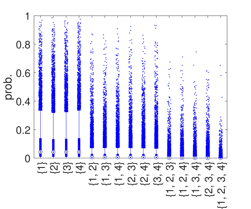
(b) A sparsity-supporting prior

Figure SD.1: Implied prior distribution over consideration sets (box plots) for two different priors on $q_{hj}$. Uniform prior (a) with $(\underline{a}_{q_{j}},\underline{b}_{q_{j}})=(1,1)$ and sparsity supporting prior (b) with $(\underline{a}_{q_{j}},\underline{b}_{q_{j}})=(sr,s(1-r))$ with $r=\frac{1}{J}$, $s=1$. $K=20.$ $(\underline{a}_{\alpha},\underline{b}_{\alpha})=(2,4)$. and 10,000 draws from the prior.

Panel (a) in Figure SD.1 shows the implied prior distribution over the consideration sets under the uniform prior on $q_{hj}$ when $J=4$. Under the uniform prior, the prior expectation of $q_{hj}=0.5$, so the prior is the same across all consideration sets and is centered around $0.5^{4}=0.0625$. Panel (b) gives results under our sparsity-supporting prior. In this case, the prior distribution shrinks to $0$ as the cardinality of the consideration set increases.

The preceding shows that the prior on the attention probabilities $\{q_{hj}\}$ induces quite different prior distributions on consideration sets. As the number of consideration sets increase exponentially in $J$, it is crucial to apply regularization to the parameter space. Our sparsity-supporting prior promotes this regularization. It favors smaller consideration sets, while maintaining positive probabilities on larger sets.

Appendix SE Simulation with $J=100$

SE.1 Large $J$

We now consider a high-dimensional scenario with $J=100$. One mechanism by which the dependence of consideration among categories can be induced is through multiple latent subpopulations of subjects having different probabilities of consideration. Within a subpopulation, considerations are independent across categories. However, marginalizing out the latent subpopulation indicator, one obtains dependence in those category considerations. We generate the data with two subpopulations. To generate the true consideration set of a given subject, we used a Bernoulli distribution with attention probability 0.05 for each category except for categories 10, 30, 50, 70, and 90 for the first subpopulation ($i=1,\ldots,50$) where the Bernoulli attention probability was set to 0.8. For the remaining subjects in the second subpopulation ($i=51,\ldots,100$), the Bernoulli probability was set at 0.05 except for categories 20, 40, 60, 80, and 100 where the probability was set to 0.8. Conditional on the true consideration sets, we generated the responses as in the case with $J=4$.

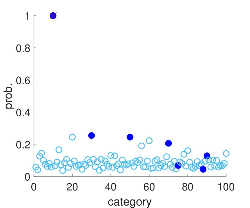
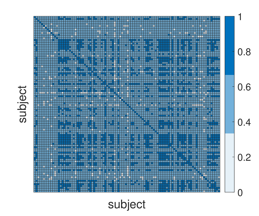
(a) $T=1$

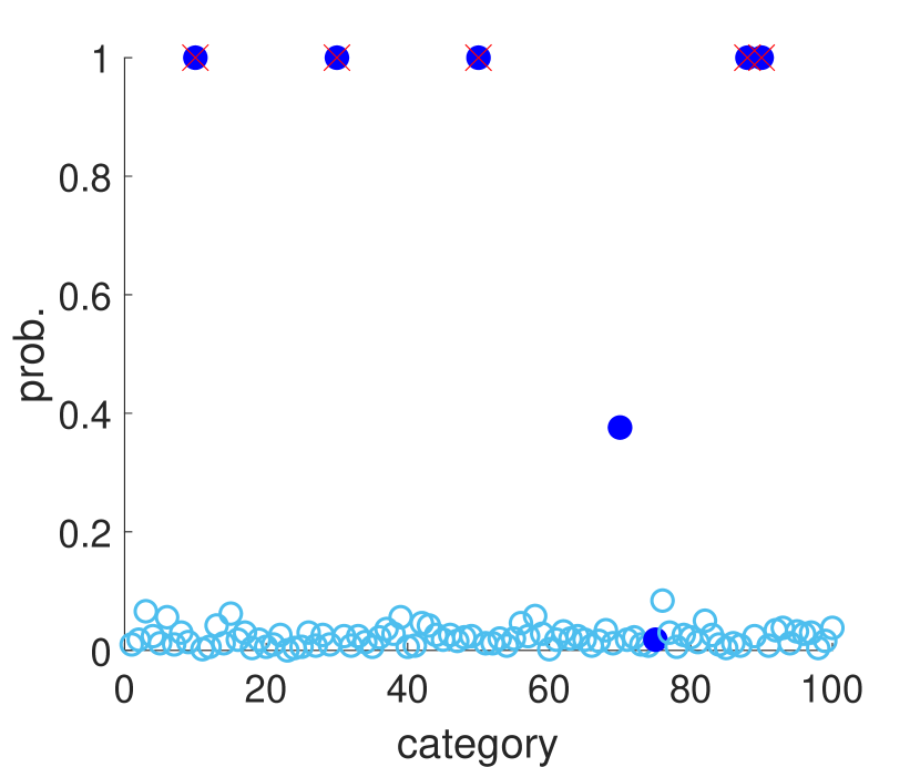
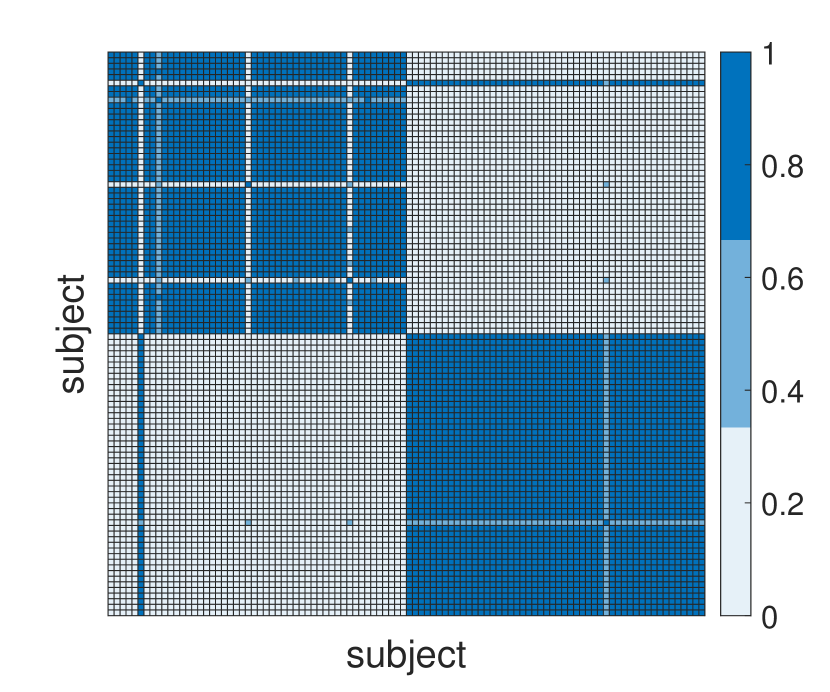
(b) $T=10$

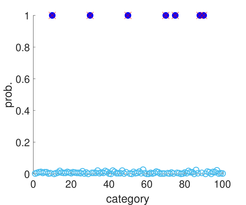
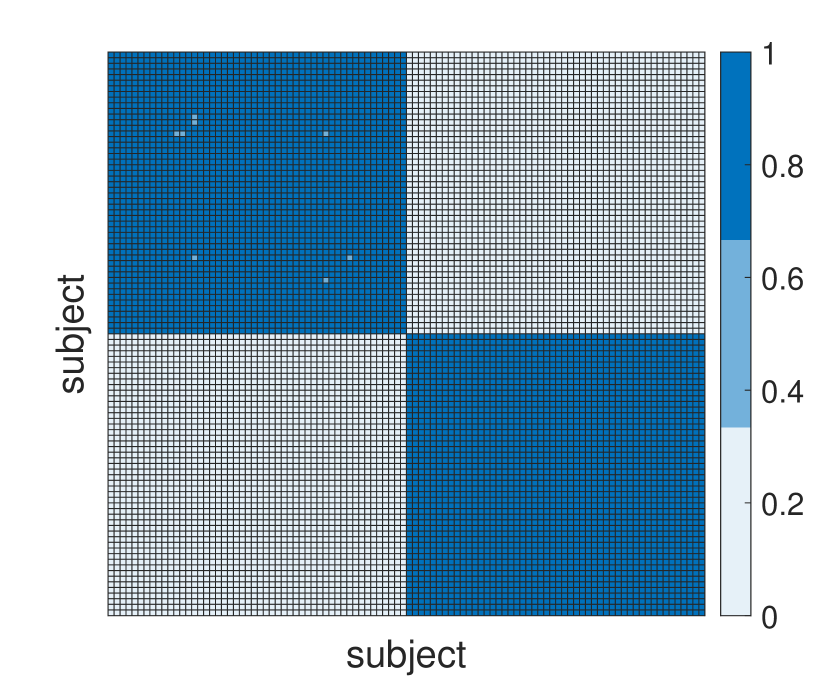
(c) $T=20$

Figure SE.1: Upper panels: Posterior mean of $1\{j\in\mathcal{C}_{1}\}$ for each item $j=1,\ldots,J$. Filled-circle if the category $j$ is within the true consideration set $\mathcal{C}_{1}^{*}=\{10,30,50,70,75,88,90\}$. Unfilled-circle if it is outside $\mathcal{C}_{1}^{*}$. A cross-sign indicates that $\exists t\leq T:y_{it}=j$. Lower panels: similarity matrices. The results are based on the simulated data with $J=100$, $T=\{1,10,20\}$, and $n=100$.

Because in this case there are $2^{100}-1$ support points in the distribution of the consideration sets, it is not possible to show the entire distribution as in Table 1. We focus on the estimation results regarding subject 1 whose true consideration set contains 7 categories: $\mathcal{C}_{1}^{*}=\{10,30,50,70,75,88,90\}$. The upper panels of Figure SE.1 show the averages of the posterior probabilities that $\mathcal{C}_{1}$ include each of the categories (filled-circle if the particular category is in the true consideration set and unfilled-circle otherwise). The lower panels of Figure SE.1 are the $n\times n$ similarity matrices. It shows the posterior probability that a given subject in a particular row $i$ is in the same cluster as another subject at a specific column $i^{\prime}$ which is computed as the posterior probability of the event $\{S_{i}=S_{i^{\prime}}\}$, which ranges from zero (light blue) to one (dark blue).

There are two remarks. First, we again see the posterior concentration toward the true consideration set as $T$ increases. Second, even when $T=1$ or $T=10$, the categories that have not yet been observed as responses by subject $1$ have relatively large posterior probabilities of being in the consideration set $\mathcal{C}_{1}$. This is because subject 1 tends to be clustered together with other subjects whose observed responses include those categories, and the estimated consideration sets are similar within the cluster.

Appendix SF Additional material for the application

SF.1 Data description

See Bronnenberg et al. (2008) for an overview of the IRI data set. The household panel data keep track of the purchase histories of brands in 30 categories for a sample of households in two cities, Eau Claire, WI and Pittsfield, MA over the years 2001–2011. For each household in the sample, the data record the timing, location and brands bought on every shopping trip to the set of stores that IRI data cover (about 80% of all the stores in the two cities). The store data contain information on quantity, price and marketing mix at store/week/UPC level. Combining household panel with store data, we could obtain the price, marketing mix for the set of UPCs that were available on shelf for the store/week at which each purchase occurred in the household panel data.

$j$	brand name	share	price	display	feature	$j$	brand name	share	price	display	feature	$j$	brand name	share	price	display	feature
1	GENERAL MILLS CHEERIOS	3.25	9.96	0.32	0.42	26	KASHI GO LEAN CRUNCH	3.10	0.87	0.34	0.19	51	POST BRAN FLAKES	3.30	1.29	0.00	0.05
2	GENERAL MILLS CINNAMON TST CR	4.20	2.09	0.24	0.31	27	KASHI HEART TO HEART	3.18	1.71	0.27	0.26	52	POST COCOA PEBBLES	3.28	0.18	0.06	0.21
3	GENERAL MILLS COCOA PUFFS	3.90	0.81	0.10	0.18	28	KELLOGGS ALL BRAN	3.76	0.87	0.04	0.14	53	POST FRUITY PEBBLES	3.45	0.48	0.15	0.21
4	GENERAL MILLS COOKIE CRISP	4.28	0.54	0.12	0.24	29	KELLOGGS ALL BRAN BRAN BUDS	4.02	0.18	0.00	0.11	54	POST GRAPE NUTS	3.41	0.96	0.05	0.13
5	GENERAL MILLS CORN CHEX	3.43	0.72	0.05	0.20	30	KELLOGGS APPLE JACKS	3.17	1.17	0.32	0.45	55	POST GRAPE NUTS TRAIL MIX CRU	3.48	0.72	0.00	0.07
6	GENERAL MILLS FIBER ONE	3.93	1.26	0.00	0.17	31	KELLOGGS CORN FLAKES	2.79	2.45	0.13	0.33	56	POST HONEY BUNCHES OF OATS	3.69	3.44	0.20	0.26
7	GENERAL MILLS FROSTED CHEERIO	4.00	0.30	0.00	0.13	32	KELLOGGS CORN POPS	3.22	1.73	0.34	0.38	57	POST HONEY NUT SHREDDED WHEAT	3.48	0.45	0.09	0.11
8	GENERAL MILLS FRUITY CHEERIOS	3.12	1.11	0.11	0.23	33	KELLOGGS CRACKLIN OAT BRAN	4.12	0.54	0.00	0.18	58	POST HONEYCOMB	3.27	0.36	0.02	0.14
9	GENERAL MILLS GOLDEN GRAHAMS	4.24	1.35	0.12	0.23	34	KELLOGGS CRISPIX	3.76	0.96	0.07	0.25	59	POST RAISIN BRAN	3.59	1.20	0.16	0.16
10	GENERAL MILLS HONEY NUT CHEER	3.87	7.84	0.28	0.39	35	KELLOGGS CRUNCHY BLENDS	3.81	0.09	0.01	0.18	60	POST SELCTS CRANBRRY ALMND CR	3.53	0.48	0.00	0.12
11	GENERAL MILLS KIX	3.28	1.20	0.07	0.17	36	KELLOGGS FROOT LOOPS	3.17	2.60	0.38	0.44	61	POST SELECTS GREAT GRAINS	3.53	0.66	0.00	0.12
12	GENERAL MILLS LUCKY CHARMS	4.22	2.06	0.23	0.25	37	KELLOGGS FROSTD MN WHTS MPL	3.75	0.60	0.09	0.16	62	POST SHREDDED WHEAT	3.74	0.60	0.00	0.02
13	GENERAL MILLS MULTI GRAIN CHE	3.76	1.94	0.04	0.21	38	KELLOGGS FROSTD MN WHTS STRWB	3.72	0.84	0.07	0.18	63	POST SPOON SIZE SHREDDED WHEA	3.37	0.66	0.10	0.11
14	GENERAL MILLS OATMEAL CRISP	4.13	0.09	0.03	0.17	39	KELLOGGS FROSTED FLAKES	3.42	5.29	0.44	0.45	64	QUAKER CAP N CRUNCH	3.65	1.05	0.11	0.11
15	GENERAL MILLS RAISIN NUT BRAN	4.19	0.24	0.00	0.17	40	KELLOGGS FROSTED MINI WHEATS	3.59	3.11	0.20	0.38	65	QUAKER CAP N CRUNCH CRUNCH BE	3.65	0.99	0.11	0.11
16	GENERAL MILLS REESES PUFFS	4.21	1.02	0.14	0.18	41	KELLOGGS FUN PAK	3.34	0.06	0.00	0.08	66	QUAKER CP N CRNCH PNT BTTR CR	3.66	0.48	0.11	0.11
17	GENERAL MILLS RICE CHEX	3.42	0.57	0.05	0.20	42	KELLOGGS RAISIN BRAN	3.28	2.84	0.26	0.38	67	QUAKER LIFE	3.73	2.42	0.09	0.06
18	GENERAL MILLS TOTAL	3.82	1.88	0.10	0.29	43	KELLOGGS RAISIN BRAN CRUNCH	3.72	1.71	0.03	0.09	68	QUAKER OATMEAL SQUARES	3.70	0.66	0.00	0.02
19	GENERAL MILLS TOTAL RAISIN BR	4.30	0.99	0.05	0.21	44	KELLOGGS RICE KRISPIES	3.15	4.91	0.40	0.46
20	GENERAL MILLS TRIX	3.49	0.87	0.13	0.18	45	KELLOGGS SMACKS	3.25	0.48	0.13	0.28
21	GENERAL MILLS WHEAT CHEX	3.43	0.90	0.04	0.20	46	KELLOGGS SMART START	3.67	0.09	0.03	0.21
22	GENERAL MILLS WHEATIES	3.56	1.76	0.09	0.15	47	KELLOGGS SMART START HEALTH	3.51	0.78	0.05	0.19
23	GENERAL MILLS YOGURT BRST CHE	3.64	0.66	0.04	0.21	48	KELLOGGS SPECIAL K	3.57	2.72	0.22	0.33
24	GENERAL MLLS APPL CINNAMN CHE	4.04	1.35	0.04	0.21	49	KELLOGGS SPECIAL K RED BERRIE	3.99	2.87	0.17	0.18
25	KASHI GO LEAN	3.08	0.51	0.34	0.19	50	KELLOGGS SPECIAL K VANILLA AL	3.54	1.50	0.13	0.15

Table SF.1: Descriptive statistics of the 68 cereal brands

SF.2 Additional estimation results and discussion

SF.2.1 Estimated parameters in the response model

Common fixed-effects

The estimation results of the fixed-effect parameters $\bm{\beta}$ from the four models are summarized in the first panel of Table 4. The signs of the estimates in these models for price and display are consistent with previous studies, and the corresponding 95% credible intervals do not include 0. In contrast, feature may not play an important role in this subsample as the 95% credible intervals include 0 in all models except for MNL.

Random-effects

We now consider estimates for the random-effects obtained from MNL_R and MNL_RC. The second panel in Table 4 reports the square root of the diagonal elements of $\bm{D}$, denoted by $D_{hh}^{1/2}$. The posterior sample of $D_{hh}^{1/2}$ is obtained from that of $\{\bm{D}^{(g)}\}$ by taking the point-wise square root of each draw. The posterior moments such as means and standard deviations are then computed based on the transformed sample. When we control for variation in consideration sets, the extent of preference parameter heterogeneity tends to diminish, which is consistent with previous study (Chiang et al. (1998)).

Brand-specific fixed-effects

Next, the number of brand-specific fixed-effects whose 95% credible intervals do not include 0 is larger for MNL than MNL_C and for MNL_R than MNL_RC. This phenomenon was also observed by Chiang et al. (1998). To explain this, we note that under MNL_C and MNL_RC, the estimated consideration sets $\{\mathcal{C}_{i}\}$ are much smaller than the set with all brands. If, for example, there is a brand that is almost never chosen by any household, the estimated $\{\mathcal{C}_{i}\}$ tends to exclude such a brand. The standard logit model does not account for such nonconsideration and instead assumes that every household considers all brands. As a result, the magnitudes of brand-specific fixed effects tend to be overestimated.

Table SF.2 shows the estimated brand-specific fixed-effects $\delta_{j}$. Under the full specification, for 13 out of 68 of them, the corresponding 95% credible interval does not include 0. Note that $\delta_{J}=0$ for identification.

Table SF.2: Estimates of the brand-specific fixed-effects from the real data on cereal market

brand	mean	s.d	brand	mean	s.d	brand	mean	s.d
GENERAL MILLS CHEERIOS	0.18	0.31	KASHI GO LEAN CRUNCH	-0.65	0.47	POST BRAN FLAKES	2.07*	0.42
GENERAL MILLS CINNAMON TST CR	0.14	0.31	KASHI HEART TO HEART	0.42	0.39	POST COCOA PEBBLES	-1.79*	0.67
GENERAL MILLS COCOA PUFFS	-0.44	0.4	KELLOGGS ALL BRAN	0.33	0.40	POST FRUITY PEBBLES	-1.03	0.54
GENERAL MILLS COOKIE CRISP	0.00	0.52	KELLOGGS ALL BRAN BRAN BUDS	-1.23	0.93	POST GRAPE NUTS	-0.06	0.39
GENERAL MILLS CORN CHEX	-0.33	0.41	KELLOGGS APPLE JACKS	-0.04	0.36	POST GRAPE NUTS TRAIL MIX CRU	-0.19	0.43
GENERAL MILLS FIBER ONE	0.46	0.38	KELLOGGS CORN FLAKES	-0.46	0.29	POST HONEY BUNCHES OF OATS	0.21	0.31
GENERAL MILLS FROSTED CHEERIO	-0.21	0.72	KELLOGGS CORN POPS	-0.25	0.34	POST HONEY NUT SHREDDED WHEAT	-1.30	0.65
GENERAL MILLS FRUITY CHEERIOS	-0.12	0.37	KELLOGGS CRACKLIN OAT BRAN	0.37	0.67	POST HONEYCOMB	-1.14*	0.57
GENERAL MILLS GOLDEN GRAHAMS	-0.07	0.36	KELLOGGS CRISPIX	-0.41	0.41	POST RAISIN BRAN	-0.45	0.44
GENERAL MILLS HONEY NUT CHEER	0.50	0.29	KELLOGGS CRUNCHY BLENDS	-3.42*	1.17	POST SELCTS CRANBRRY ALMND CR	-0.89	0.54
GENERAL MILLS KIX	-0.27	0.40	KELLOGGS FROOT LOOPS	-0.00	0.31	POST SELECTS GREAT GRAINS	-0.06	0.97
GENERAL MILLS LUCKY CHARMS	0.35	0.32	KELLOGGS FROSTD MN WHTS MPL	0.39	0.46	POST SHREDDED WHEAT	-0.88	0.65
GENERAL MILLS MULTI GRAIN CHE	0.52	0.41	KELLOGGS FROSTD MN WHTS STRWB	0.26	0.39	POST SPOON SIZE SHREDDED WHEA	-2.14*	0.54
GENERAL MILLS OATMEAL CRISP	-2.52*	1.04	KELLOGGS FROSTED FLAKES	0.12	0.31	QUAKER CAP N CRUNCH	0.35	0.37
GENERAL MILLS RAISIN NUT BRAN	-1.93*	0.79	KELLOGGS FROSTED MINI WHEATS	0.23	0.33	QUAKER CAP N CRUNCH CRUNCH BE	0.97*	0.43
GENERAL MILLS REESES PUFFS	0.27	0.39	KELLOGGS FUN PAK	-3.00*	1.09	QUAKER CP N CRNCH PNT BTTR CR	-0.19	0.79
GENERAL MILLS RICE CHEX	-0.50	0.49	KELLOGGS RAISIN BRAN	-0.10	0.37	QUAKER LIFE	0.10	0.29
GENERAL MILLS TOTAL	0.50	0.33	KELLOGGS RAISIN BRAN CRUNCH	1.57*	0.33	QUAKER OATMEAL SQUARES	0.00	NaN
GENERAL MILLS TOTAL RAISIN BR	-0.24	0.43	KELLOGGS RICE KRISPIES	-0.09	0.35
GENERAL MILLS TRIX	0.36	0.42	KELLOGGS SMACKS	-1.24*	0.55
GENERAL MILLS WHEAT CHEX	1.03	0.52	KELLOGGS SMART START	-3.29*	1.31
GENERAL MILLS WHEATIES	-0.21	0.33	KELLOGGS SMART START HEALTHY	-0.56	0.51
GENERAL MILLS YOGURT BRST CHE	-0.68	0.62	KELLOGGS SPECIAL K	0.22	0.36
GENERAL MLLS APPL CINNAMN CHE	0.38	0.36	KELLOGGS SPECIAL K RED BERRIE	1.01*	0.34
KASHI GO LEAN	-0.96	0.52	KELLOGGS SPECIAL K VANILLA AL	0.53	0.38

• The stars indicate that the corresponding 95% credible interval does not include 0.

SF.2.2 Estimated parameters in the mixture model

Below, we present additional estimation results concerning the parameters in the mixture model under the MNL_RC specification. Figure SF.1 compares the prior and posterior densities of the DP concentration parameter $\alpha$. The Gamma prior $\alpha\sim Gamma(2,4)$ density is shown as the dashed line and the posterior is shown in the solid line.

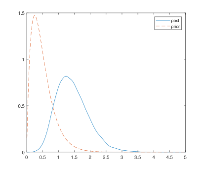
Figure SF.1: pdf’s of $\alpha$: prior (dashed) and posterior (solid) from the empirical application. MNL_RC.

Figure SF.2 shows the posterior probability mass function of the non-empty mixture components. The posterior mode of the number of non-empty components is 7.

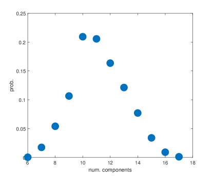
Figure SF.2: Posterior probability mass function of the number of nonempty components from the empirical application. MNL_RC.

References

- Abaluck and Adams-Prassl (2021) J. Abaluck and A. Adams-Prassl. What do consumers consider before they choose? identification from asymmetric demand responses. The Quarterly Journal of Economics, 136(3):1611–1663, 2021.
- Aguiar et al. (2023) V. H. Aguiar, M. J. Boccardi, N. Kashaev, and J. Kim. Random utility and limited consideration. Quantitative Economics, 14(1):71–116, 2023.
- Barseghyan et al. (2021) L. Barseghyan, M. Coughlin, F. Molinari, and J. C. Teitelbaum. Heterogeneous choice sets and preferences. Econometrica, 89(5):2015–2048, 2021.
- Ben-Akiva and Boccara (1995) M. Ben-Akiva and B. Boccara. Discrete choice models with latent choice sets. International Journal of Research in Marketing, 12(1):9–24, 1995.
- Bronnenberg et al. (2008) B. J. Bronnenberg, M. W. Kruger, and C. F. Mela. Database paper—the iri marketing data set. Marketing science, 27(4):745–748, 2008.
- Cattaneo et al. (2020) M. D. Cattaneo, X. Ma, Y. Masatlioglu, and E. Suleymanov. A random attention model. Journal of Political Economy, 128(7):2796–2836, 2020.
- Chiang et al. (1998) J. Chiang, S. Chib, and C. Narasimhan. Markov chain monte carlo and models of consideration set and parameter heterogeneity. Journal of Econometrics, 89(1-2):223–248, 1998.
- Chib and Greenberg (1995) S. Chib and E. Greenberg. Understanding the metropolis-hastings algorithm. The American Statistician, 49(4):327–335, 1995.
- Chib and Greenberg (1998) S. Chib and E. Greenberg. Analysis of multivariate probit models. Biometrika, 85(2):347–361, 1998.
- Crawford et al. (2021) G. S. Crawford, R. Griffith, and A. Iaria. A survey of preference estimation with unobserved choice set heterogeneity. Journal of Econometrics, 222(1):4–43, 2021.
- Devroye et al. (2018) L. Devroye, A. Mehrabian, and T. Reddad. The total variation distance between high-dimensional gaussians with the same mean. arXiv preprint arXiv:1810.08693, 2018.
- Dunson and Xing (2009) D. B. Dunson and C. Xing. Nonparametric bayes modeling of multivariate categorical data. Journal of the American Statistical Association, 104(487):1042–1051, 2009.
- Escobar and West (1995) M. D. Escobar and M. West. Bayesian density estimation and inference using mixtures. Journal of the American Statistical Association, 90(430):577–588, 1995.
- Ferguson (1973) T. S. Ferguson. A bayesian analysis of some nonparametric problems. The Annals of Statistics, pages 209–230, 1973.
- Goeree (2008) M. S. Goeree. Limited information and advertising in the us personal computer industry. Econometrica, 76(5):1017–1074, 2008.
- Kawaguchi et al. (2021) K. Kawaguchi, K. Uetake, and Y. Watanabe. Designing context-based marketing: Product recommendations under time pressure. Management Science, 2021.
- Lu (2022) Z. Lu. Estimating multinomial choice models with unobserved choice sets. Journal of Econometrics, 226(2):368–398, 2022.
- Manski (1977) C. F. Manski. The structure of random utility models. Theory and decision, 8(3):229, 1977.
- Manzini and Mariotti (2014) P. Manzini and M. Mariotti. Stochastic choice and consideration sets. Econometrica, 82(3):1153–1176, 2014.
- Norets and Pelenis (2014) A. Norets and J. Pelenis. Posterior consistency in conditional density estimation by covariate dependent mixtures. Econometric Theory, 30(3):606–646, 2014.
- Norets and Shimizu (2022) A. Norets and K. Shimizu. Semiparametric bayesian estimation of dynamic discrete choice models. Under Review. arXiv preprint arXiv:2202.04339, 2022.
- Paleti et al. (2021) R. Paleti, S. Mishra, K. Haque, and M. M. Golias. Latent class analysis of residential and work location choices. Transportation Letters, 13(10):696–706, 2021.
- Sethuraman (1994) J. Sethuraman. A constructive definition of dirichlet priors. Statistica Sinica, pages 639–650, 1994.
- Swait and Ben-Akiva (1987) J. Swait and M. Ben-Akiva. Incorporating random constraints in discrete models of choice set generation. Transportation Research Part B: Methodological, 21(2):91–102, 1987.
- Traets et al. (2022) F. Traets, M. Meulders, and M. Vandebroek. Modelling consideration heterogeneity in a two-stage conjunctive model. Journal of Mathematical Psychology, 109:102687, 2022.
- Van Nierop et al. (2010) E. Van Nierop, B. Bronnenberg, R. Paap, M. Wedel, and P. H. Franses. Retrieving unobserved consideration sets from household panel data. Journal of Marketing Research, 47(1):63–74, 2010.
- Walker (2007) S. G. Walker. Sampling the dirichlet mixture model with slices. Communications in Statistics—Simulation and Computation®, 36(1):45–54, 2007.