Diffuse, Attend, and Segment: Unsupervised Zero-Shot Segmentation using Stable Diffusion

Abstract

Producing quality segmentation masks for images is a fundamental problem in computer vision. Recent research has explored large-scale supervised training to enable zero-shot segmentation on virtually any image style and unsupervised training to enable segmentation without dense annotations. However, constructing a model capable of segmenting anything in a zero-shot manner without any annotations is still challenging. In this paper, we propose to utilize the self-attention layers in stable diffusion models to achieve this goal because the pre-trained stable diffusion model has learned inherent concepts of objects within its attention layers. Specifically, we introduce a simple yet effective iterative merging process based on measuring KL divergence among attention maps to merge them into valid segmentation masks. The proposed method does not require any training or language dependency to extract quality segmentation for any images. On COCO-Stuff-27, our method surpasses the prior unsupervised zero-shot SOTA method by an absolute $26\%$ in pixel accuracy and $17\%$ in mean IoU. The project page is at https://sites.google.com/view/diffseg/home.

1 Introduction

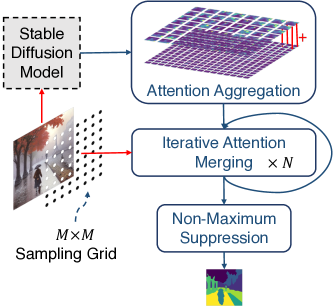
Figure 1: Overview of DiffSeg. DiffSeg is an unsupervised and zero-shot segmentation algorithm using a pre-trained stable diffusion model. Starting from $M\times M$ anchor points, DiffSeg iteratively merges self-attention maps from the diffusion model for $N$ iterations to segment any image without any prior knowledge and external information.

Semantic segmentation divides an image into regions of entities sharing the same semantics. It is an important foundational application for many downstream tasks such as image editing [26], medical imaging [27], and autonomous driving [13] etc. While supervised semantic segmentation, where a target dataset is available and the categories are known, has been widely studied [39, 37, 9], zero-shot segmentation for any images with unknown categories is much more challenging. A recent popular work SAM [20], trains a neural network on 1.1B segmentation annotations and achieves impressive zero-shot transfer to any images. This is an important step towards making segmentation a more flexible foundation task for many other tasks, not just limited to a given dataset with limited categories. However, the cost of collecting per-pixel labels is high. Therefore, it is of high research and production interest to investigate unsupervised and zero-shot segmentation methods under the least restrictive settings, i.e., no form of annotations and no prior knowledge of the target.

Few works have taken up the challenge due to the combined difficulty of the unsupervised and zero-shot requirements. For example, most works in unsupervised segmentation require access to the target data for unsupervised adaption [14, 41, 24, 36, 15, 11, 18]. Therefore, these methods cannot segment images that are not seen during the adaptation. Recently, ReCo [35] proposed a retrieve-and-co-segment strategy. It removes the requirement for supervision because it uses an unsupervised vision backbone, e.g., DINO [8], and is zero-shot since it does not need training on the target distribution of images. Still, to satisfy these requirements, ReCo needs to 1) identify the concept beforehand and 2) maintain a large pool of unlabelled images for retrieval. This is still far from the capability of SAM [20], which does not require knowledge of the target image and any auxiliary information.

To move towards the goal, we propose to utilize the power of a stable diffusion (SD) model [33] to construct a general segmentation model. Recently, stable diffusion models have been used on generating prompt-conditioned high-resolution images [33]. It is reasonable to hypothesize that there exists information on object groupings in a diffusion model. For example, DiffuMask [38] discovers that the cross-attention layer contains explicit object-level pixel groupings when cross-referenced between the produced attention maps and the input prompt. However, DiffuMask can only produce segmentation masks for a generated image with a corresponding text prompt and is limited to dominant foreground objects explicitly referred to by the prompt. Motivated by this, we investigate the unconditioned self-attention layer in a diffusion model. We observed that the attention tensors from the self-attention layers contain specific spatial relationships: Intra-Attention Similarity and Inter-Attention Similarity (Sec. 3.1). Relying on these two properties, it is possible to uncover segmentation masks for any objects in an image.

To this end, we propose DiffSeg (Sec. 3.2), a simple yet effective post-processing method, for producing segmentation masks by using the attention tensors generated by the self-attention layers in a diffusion model solely. The algorithm consists of three main components: attention aggregation, iterative attention merging and non-maximum suppression as shown in Fig. 1. Specifically, DiffSeg aggregates the 4D attention tensors in a spatially consistent manner to preserve visual information across multiple resolutions and uses an iterative merging process by first sampling a grid of anchor points. The sampled anchors provide starting points for merging attention masks, where anchors in the same object are absorbed eventually. The merging process is controlled by measuring the similarity between two attention maps using KL divergence. Unlike, popular clustering-based unsupervised segmentation methods [11, 15, 24], DiffSeg does not require specifying the number of clusters beforehand and is also deterministic. Given an image, without any prior knowledge, DiffSeg can produce a quality segmentation without resorting to any additional resources (e.g. as SAM requires). We benchmark DiffSeg on the popular unsupervised segmentation dataset COCO-Stuff-27 and a specialized self-driving dataset Cityscapes. DiffSeg outperforms prior works on both datasets despite requiring less auxiliary information during inference. In summary,

• We propose an unsupervised and zero-shot segmentation method, DiffSeg, using a pre-trained stable diffusion model. DiffSeg can segment images in the wild without any prior knowledge or additional resources.

• DiffSeg sets new state-of-the-art performance on two segmentation benchmarks. On COCO-Stuff-27, our method surpasses a prior unsupervised zero-shot SOTA method by an absolute $26\%$ in pixel accuracy and $17\%$ in mean IoU.

2 Related Works

Diffusion Models. Our work builds on pre-trained diffusion models [17, 33, 34]. The diffusion model is a popular generative model for computer vision applications. It learns a forward and reverse diffusion process to generate an image from a sampled isotropic Gaussian noise image [17]. The most popular variant is the latent (stable) diffusion model [33]. Many existing works have studied the discriminative visual features in a diffusion model and used it for zero-shot classification [22], supervised segmentation [3], label-efficient segmentation [5], semantic-correspondence matching [16, 42] and open-vocabulary segmentation [40]. They rely on the high-dimensional visual features learned in stable diffusion models to perform those tasks, which require them to add additional training to take full advantage of those features. Instead, we show that object grouping is also an emergent property of the self-attention layer in the Transformer module manifested in 4-dimensional spatial attention tensors with special spatial patterns.

Unsupervised Segmentation. Our work is closely related to unsupervised segmentation [14, 41, 24, 36, 15, 11, 18]. This line of works aims to generate dense segmentation masks without using any annotations. However, they generally require unsupervised training on the target dataset to achieve good performance. We characterize the most recent works into two main categories: clustering based on invariance [11, 18] and clustering using pre-trained models [41, 24, 15, 36]. In the first category, IIC [18] is a generic clustering algorithm that segments images into semantic clusters by optimizing the mutual information between a pair of images to avoid degenerate segmentation. PiCLE [11] explores pixel-level invariant and equivariant constraints and trains a segmentation network to enforce the consistency of these constraints. More recently, research has been shifted to utilize large self-supervised vision models such as DINO [8]. These new works utilize the discriminative features learned in those pre-trained models, i.e., features from the same semantic class are generally more similar, to produce segmentation masks. STEGO [15] learns a non-linear projection layer to amplify and “distill” the correlation in pre-trained models. ACseg [24] learns to feature prototypes to automatically discover clusters in the feature space of a pre-trained model. COMUS [41] uses an external saliency map detector, e.g., DeepUSPS [30], to generate coarse object proposals and refine the proposal using features from pre-trained vision models to generate pseudo-masks. A subsequent segmentation network is trained using the refined pseudo-masks. More closely related to ours, DiffuMasks [38] uses the cross-modal grounding between the text prompt and the image in the cross-attention layer of a diffusion model to segment the most prominent object, referred by the text prompt, in the synthetic image. However, DiffuMasks can only be applied to a generated image. In contrast, our method applies to any real images without the requirement of a text prompt.

Zero-Shot Segmentation Another related field is zero-shot segmentation [20, 35, 29, 6, 38, 14, 44]. Works in this line of work possess the capability of “segmenting anything” without any training. Most recently, SAM [20], trained on 1.1B segmentation masks, demonstrated impressive zero-shot transfer to any images. MaskCLIP [44] and CLIPSeg [29] extend CLIP to provide segmentation based on an image and text input by training an additional segmentation network. Most similar to our work are Network-Free [14] and ReCo [35]. Network-Free [14] uses a pre-trained StyleGAN [19] to produce segmentation masks. Specifically, it uses StyleGAN to generate multiple synthetic images of different styles for the same content and utilize pixel-level consistency to produce a segmentation mask. ReCo [35] also operates on images with a caption describing its content. It uses both CLIP [32] and a pre-trained image encoder, e.g., MoCoV2 [10], to first retrieve a batch reference images and then uses a novel co-segmentation algorithm to segment recurring content in all images including the target and reference images. In contrast, our method uses a diffusion model to generate segmentation without synthesizing and querying multiple images, and more importantly without even knowing the objects in the image, thus removing the need for text input in ReCo.

3 Method

DiffSeg utilizes a pre-trained stable diffusion model [33] and specifically its self-attention layers to produce high-quality segmentation masks. We will briefly review the architecture of the stable diffusion model in Sec. 3.1 and introduce DiffSeg in Sec. 3.2.

3.1 Stable Diffusion Model Review

The Stable diffusion model [33] is a popular variant of the diffusion model family [17, 34], which is a type of generative model. Diffusion models have a forward and a reverse pass. In the forward pass, at every time step, a small amount of Gaussian noise is iteratively added until an image becomes an isotropic Gaussian noised image. In the reverse pass, the diffusion model is trained to iteratively remove the Gaussian noise to recover the original clean image. The stable diffusion model [33] introduces an encoder-decoder and U-Net design with attention layers [17]. It first compress an image $x\in\mathbb{R}^{H\times W\times 3}$ into a latent space with smaller spatial dimension $z\in\mathbb{R}^{h\times w\times c}$ using an encoder $z=\mathcal{E}(x)$, which can be de-compressed through a decoder $\tilde{x}=\mathcal{D}(z)$. All diffusion processes happen in the latent space through a U-Net architecture. The U-Net architecture will be the focus of investigation in this paper.

The U-Net architecture [33] consists of a stack of modular blocks (a schematic is provided in Appendix 8.1). Among those blocks, there are 16 specific blocks which are composed of two major components: a ResNet layer and a Transformer layer. The Transformer layer uses two types of attention mechanisms: self-attention to learn the global attention across the image and cross-attention to learn attention between the image and optional text input. The component of interest for our investigation is the self-attention layer in the Transformer layer. Specifically, there are a total of $16$ self-attention layers distributed in the 16 composite blocks, giving 16 self-attention tensors:

$$\mathcal{A}\in\{\mathcal{A}_{k}\in\mathbb{R}^{h_{k}\times w_{k}\times h_{k}\times w_{k}}|k=1,...,16\}.$$ (1)

Each attention tensor $\mathcal{A}_{k}$ is 4-dimensional. Inspired by DiffuMask [38], which demonstrates object grouping in the cross-attention layer, where salient objects are given more attention when referred by its corresponding text input, we hypothesize that the unconditional self-attention also contains inherent object grouping information and can be used to produce segmentation masks without text inputs.

Specifically, for each spatial location $(I,J)$ in the attention tensor, the corresponding 2D attention map $\mathcal{A}_{k}[I,J,:,:]\in\mathbb{R}^{h_{k}\times w_{k}}$ captures the semantic correlation between all locations and the location $(I,J)$. Each location $(I,J)$ corresponds to a region in the original image pixel space, the size of which depends on the receptive field of the tensor.

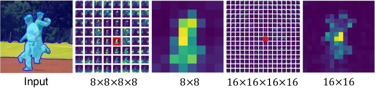
Figure 2: Visualization of Segmentation Masks and Self-Attentions Tensors. Left: Overlay of segmentation and the original image. Right: Attention maps from a stable diffusion model have two properties: Intra-Attention Similarity and Inter-Attention Similarity. Maps of different resolutions have varying receptive fields w.r.t the original image.

To illustrate this, we visualize the self-attention tensors $A_{7}$ and $\mathcal{A}_{8}$ in Fig. 2. They have a dimension of $\mathcal{A}_{7}\in\mathbb{R}^{8^{4}}$ and $\mathcal{A}_{8}\in\mathbb{R}^{16^{4}}$ respectively. There are two important observations that will motivate our method in Sec. 3.2.

• Intra-Attention Similarity: Within a 2D attention map $\mathcal{A}_{k}[I,J,:,:]$, locations tend to have strong responses if they correspond to the same object group as $(I,J)$ in the original image space, e.g., $\mathcal{A}_{k}[I,J,I+1,J+1]$ is likely to be a large value.

• Inter-Attention Similarity: Between two 2D attention maps, e.g., $\mathcal{A}_{k}[I,J,:,:]$ and $\mathcal{A}_{k}[I+1,J+1,:,:]$, they tend to share similar activations if $(I,J)$ and $(I+1,J+1)$ belong to the same object group in the original image space.

The second observation is a direct consequence of the first one. In general, we found that attention maps tend to focus on object groups, i.e., groups of individual objects sharing similar visual features (see segmentation examples in Fig. 6). In this example (Fig. 2), the two people are grouped as a single object group. The $8\times 8$ resolution map from a location inside the group highlights a large portion of the entire group whereas the $16\times 16$ resolution map from a location also inside the object highlights a smaller portion.

Theoretically, the resolution of the attention map dictates the size of its receptive field w.r.t the original image. A smaller resolution leads to a larger respective field, corresponding to a larger portion of the original image. Practically, lower resolution maps, e.g., $8\times 8$ provide a better grouping of large objects as a whole and larger resolution maps e.g., $16\times 16$ provide a more fine-grained grouping of components in larger objects and potentially are better for identifying small objects. Overall, the current stable diffusion model has attention maps in 4 resolutions $(h_{k},w_{k})\in\{8\times 8,16\times 16,32\times 32,64\times 64\}$. Building on these observations, in the next section, we will propose a simple heuristic to aggregate weights from different resolutions and introduce an iterative method to merge all attention maps into a valid segmentation.

A Note on Extracting Attention Maps. In our experiments, we use the stable diffusion pre-trained models from Huggingface. These are prompt-conditioned diffusion models and normally run for $\geq 50$ diffusion steps to generate new images. However, in our case, we want to extract attention maps for an existing clean image without conditional prompt efficiently. We achieve this by 1) using only the unconditioned latent and 2) only running the diffusion process once. The unconditional latent is calculated using an unconditioned text embedding. Since we only do one pass through the diffusion model, we also set the time-step variable $t$ to a large value e.g., $t=300$ in our experiments such that the real images are viewed as mostly denoised generated images from the perspective of the diffusion model.

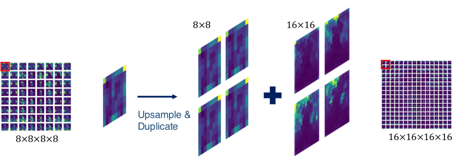
(a) Example of Attention Aggregation. An attention map from a lower resolution is first upsampled and then duplicated to match the receptive field of the higher-resolution maps.

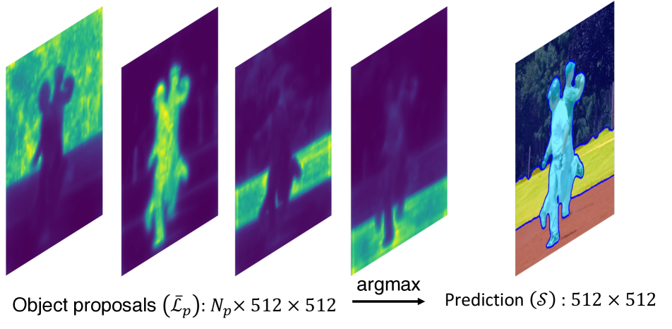
(b) Example of Non-Maximum Suppression (NMS). NMS looks up the maximum activation across the $\mathcal{L}_{p}$ proposals for each pixel.

Figure 3:

3.2 DiffSeg

Since the self-attention layers capture inherent object grouping information in the form of spatial attention (probability) maps, we propose DiffSeg, a simple post-processing method, to aggregate and merge attention tensors into a valid segmentation mask. The pipeline mainly consists of three components: attention aggregation, iterative attention merging, and non-maximum suppression shown in Fig. 1. We will introduce each component in detail next.

Attention Aggregation. Given an input image passing through the encoder and U-Net, a stable diffusion model generates 16 attention tensors. Specifically, there are 5 tensors for each of the dimensions: $64\times 64\times 64\times 64$, $32\times 32\times 32\times 32$, $16\times 16\times 16\times 16$, $8\times 8\times 8\times 8$; and 1 tensor for the dimension $8\times 8\times 8\times 8$. The goal is to aggregate attention tensors of different resolutions into the highest resolution tensor. To achieve this, we need to carefully treat the 4 dimensions differently.

As discussed in the previous section, the 2D map $\mathcal{A}_{k}[I,J,:,:]$ corresponds to the correlation between all spatial locations and the location $(I,J)$. Therefore, the last 2 dimensions in the attention tensors are spatially consistent despite different resolutions. Therefore, we upsample (bi-linear interpolation) the last 2 dimensions of all attention maps to $64\times 64$, the highest resolution of them. Formally, for $\mathcal{A}_{k}\in\mathbb{R}^{h_{k}\times w_{k},\times h_{k}\times w_{k}}$,

$$\tilde{\mathcal{A}}_{k}=\text{Bilinear-upsample}(\mathcal{A}_{k})\in\mathbb{R}^{h_{k}\times w_{k}\times 64\times 64}.$$ (2)

On the other hand, the first 2 dimensions indicate the locations to which attention maps are referenced to. Therefore, we need to aggregate attention maps accordingly. For example, as shown in Fig. 3(a), the attention map in the $(0,0)$ location in $\mathcal{A}_{k}\in\mathbb{R}^{8^{4}}$ is first upsampled and then repeatedly aggregated pixel-wise with the 4 attention maps $(0,0),(0,1),(1,0),(1,1)$ in $\mathcal{A}_{z}\in\mathbb{R}^{16^{4}}$. Formally, the final aggregated attention tensor $\mathcal{A}_{f}\in\mathbb{R}^{64^{4}}$ is,

$$\mathcal{A}_{f}[I,J,:,:] =\sum_{k\in\{1,...,16\}}\tilde{\mathcal{A}}_{k}[I/\delta_{k},J/\delta_{k},:,:]*R_{k},$$ (3)

$$\text{where}\quad\delta_{k}=64/w_{k},\quad\sum_{k}R_{k}=1.$$

where $/$ denotes floor division here. Furthermore, to ensure that the aggregated attention map is also a valid distribution, i.e., $\sum\mathcal{A}_{f}[I,J,:,:]=1$, we normalize $\mathcal{A}_{f}[I,J,:,:]$ after aggregation. $R_{k}$ is the aggregation importance ratio for each attention map. We assign every attention map of different resolutions a weight proportional to its resolution $R_{k}\propto w_{k}$. We call this the proportional aggregation scheme (Propto.). The weights $R$ are important hyper-parameters and we conduct a detailed study of them in Appendix 8.5.

Iterative Attention Merging. In the previous step, the algorithm computes an attention tensor $\mathcal{A}_{f}\in\mathbb{R}^{64^{4}}$. In this section, the goal is to merge the $64\times 64$ attention maps in the tensor $\mathcal{A}_{f}$ to a stack of object proposals where each proposal likely contains the activation of a single object or stuff category. The naive solution is to run a K-means algorithm on $\mathcal{A}_{f}$ to find clusters of objects following existing works in unsupervised segmentation [11, 15, 24]. However, the K-means algorithm requires the specification of the number of clusters. This is not an intuitive hyper-parameter to tune because our goal is to segment any image in the wild. Moreover, the K-means algorithm is stochastic depending on the initialization. Each run can have a drastically different result for the same image. To highlight these limitations, we compare them with K-Means baselines in our experiments.

Instead, we propose to generate a sampling grid from which the algorithm can iteratively merge attention maps to create the proposals. Specifically, as shown in Fig. 1, in the sampling grid generation step, a set of $M\times M$ ($1\leq M\leq 64$) evenly spaced anchor points are generated $\mathcal{M}=\{(i_{m},j_{m})|m=1,...,M^{2}\}$. We then sample the corresponding attention maps from the tensor $\mathcal{A}_{f}$. This operation yields a list of $M^{2}$ 2D attention maps as anchors,

$$\mathcal{L}_{a}=\{\mathcal{A}_{f}[i_{m},j_{m},:,:]\in\mathbb{R}^{64\times 64}|(i_{m},j_{m})\in\mathcal{M}\}.$$ (4)

Since our goal is to merge attention maps to find the maps most likely containing an object, we rely on the two observations in Sec. 3.1. Specifically, when iteratively merging “similar” maps, Intra-Attention Similarity reinforces the activation of an object and Inter-Attention Similarity grows the activation to include as many pixels of the same object within the merged map. To measure similarity, we use KL divergence to calculate the “distance” between two attention maps, since each attention map $\mathcal{A}_{f}[i,j,:,:]$ (abbrev. $\mathcal{A}_{f}[i,j]$) is a valid probability distribution. Formally,

$$2*D(\mathcal{A}_{f}[i,j],\mathcal{A}_{f}[y,z])$$ (5)

$$=\left(\mathrm{KL}(\mathcal{A}_{f}[i,j]\|\mathcal{A}_{f}[y,z])+\mathrm{KL}(\mathcal{A}_{f}[yz,z]\|\mathcal{A}_{f}[i,j])\right).$$

We use both the forward and reverse KL to address the asymmetry in KL divergence. Intuitively, a small $\mathcal{D}(\cdot)$ indicates high similarity between two attention maps and that the union of them is likely to better represent the object they both belong to.

Then we start the $N$ iterations of the merging process. In the first iteration, we compute the pair-wise distance between each element in the anchor list and all attention maps using $\mathcal{D}(\cdot)$. We introduce a threshold hyper-parameter $\tau$ and for each element in the list, we average all attention maps with a distance smaller than the threshold, effectively taking the union of attention maps likely belonging to the same object that the anchor point belongs to. All merged attention maps are stored in a new proposal list $\mathcal{L}_{p}$.

Note that the first iteration does not reduce the number of proposals compared to the number of anchors. From the second iteration onward, the algorithm starts merging maps and reducing the number of proposals simultaneously by computing the distance between an element from the proposal list $\mathcal{L}_{p}$ and all elements from the same list, and merging elements with distance smaller than $\tau$ without replacement. The full iterative attention merging algorithm is provided in Alg. 1 (Appendix 8.3).

Non-Maximum Suppression. The iterative attention merging step yields a list $\mathcal{L}_{p}\in\mathbb{R}^{N_{p}\times 64\times 64}$ of $N_{p}$ object proposals in the form of attention maps (probability maps). Each proposal in the list potentially contains the activation of a single object. To convert the list into a valid segmentation mask, we use non-maximum suppression (NMS). This can be easily done since each element is a probability distribution map. We can simply take the index of the largest probability at each spatial location across all maps and assign the membership of that location to the index of the corresponding map. An example is shown in Fig. 3(b). Note that, before NMS, we first upsample all elements in $\mathcal{L}_{p}$ to the original resolution. Formally, the final segmentation mask $\mathcal{S}\in\mathbb{R}^{512\times 512}$ is

$$\bar{\mathcal{L}}_{p} =\text{Bilinear-upsample}(\mathcal{L}_{p})\in\mathbb{R}^{N_{p}\times 512\times 512}$$ (6)

$$\mathcal{S}[i,j] =\operatorname*{arg\,max}\bar{\mathcal{L}}_{p}[:,i,j]\quad\forall i,j\in\{0,...,511\}.$$

4 Experiments

Datasets. Following existing works in unsupervised segmentation [18, 7, 11, 15, 44, 35], we use two popular segmentation benchmarks, COCO-Stuff-27 [12, 11, 18] and Cityscapes [12]. COCO-stuff-27 [11, 18] is a curated version of the original COCO-stuff dataset [12]. Specifically, COCO-stuff-27 merges the 80 things and 91 stuff categories in COCO-stuff into 27 mid-level categories. We evaluate our method on the validation split curated by prior works [11, 18]. Cityscapes [12] is a self-driving dataset with 27 categories. We evaluate the official validation split. For both datasets, we report results for both the diffusion-model-native $512\times 512$ input resolution and a lower $320\times 320$ resolution following prior works.

Metrics. Following prior works [18, 7, 11, 15, 44, 35], we use pixel accuracy (ACC) and mean intersection over union (mIoU) to measure segmentation performance. Because our method does not provide a semantic label, we resort to the Hungarian matching algorithm [21] to assign each predicted mask to a ground truth mask. When there are more predicted masks than ground truth masks, the unmatched predicted masks will be taken into account as false negatives. In addition to the metrics, we also highlight the requirements participating works need to run inference. Specifically, we emphasize unsupervised adaptation (UA), language dependency (LD), and auxiliary image (AX). UA means that the specific method requires unsupervised training on the target dataset. This is common in the unsupervised segmentation literature. Methods without the UA requirement are considered zero-shot. LD means that the method requires text input such as a descriptive sentence for the image, to facilitate segmentation. AX means that the method requires additional image inputs either in the form of a pool of reference images or synthetic images.

Models. DiffSeg builds on pre-trained stable diffusion models. We use stable diffusion V1.4 [2].

4.1 Main Results

	Requirements			Metrics
Model	LD	AX	UA	ACC.	mIoU
IIC [18]	✗	✗	✓	21.8	6.7
MDC [7]	✗	✗	✓	32.3	9.8
PiCLE [11]	✗	✗	✓	48.1	13.8
PiCLE+H [11]	✗	✗	✓	50.0	14.4
STEGO [15]	✗	✗	✓	56.9	28.2
ACSeg [24]	✓	✗	✓	-	28.1
MaskCLIP [44]	✓	✗	✗	32.2	19.6
ReCo [35]	✓	✓	✗	46.1	26.3
K-Means-C (512)	✗	✗	✗	58.9	33.7
K-Means-S (512)	✗	✗	✗	62.6	34.7
Ours: DiffSeg (320)	✗	✗	✗	72.5	43.0
Ours: DiffSeg (512)	✗	✗	✗	72.5	43.6

Table 1: Evaluation on COCO-Stuff-27. Language Dependency (LD), Auxiliary Images (AX), Unsupervised Adaptation (UA). We additionally present baseline results using K-Means. K-Means-C (constant) uses a constant number of clusters, 6. K-means-S (specific) uses a specific number of clusters for each image based on the ground truth. The K-Means results use $512\times 512$ resolution.

	Requirements			Metrics
Model	LD	AX	UA	ACC.	mIoU
IIC [18]	✗	✗	✓	47.9	6.4
MDC [7]	✗	✗	✓	40.7	7.1
PiCLE [11]	✗	✗	✓	65.5	12.3
STEGO [15]	✗	✗	✓	73.2	21.0
MaskCLIP [44]	✓	✗	✗	35.9	10.0
ReCo [35]	✓	✓	✗	74.6	19.3
Ours: DiffSeg (320)	✗	✗	✗	67.3	15.2
Ours: DiffSeg (512)	✗	✗	✗	76.0	21.2

Table 2: Evaluation on Cityscapes. Language Dependency (LD), Auxiliary Images (AX), Unsupervised Adaptation (UA).

(a) Proportional

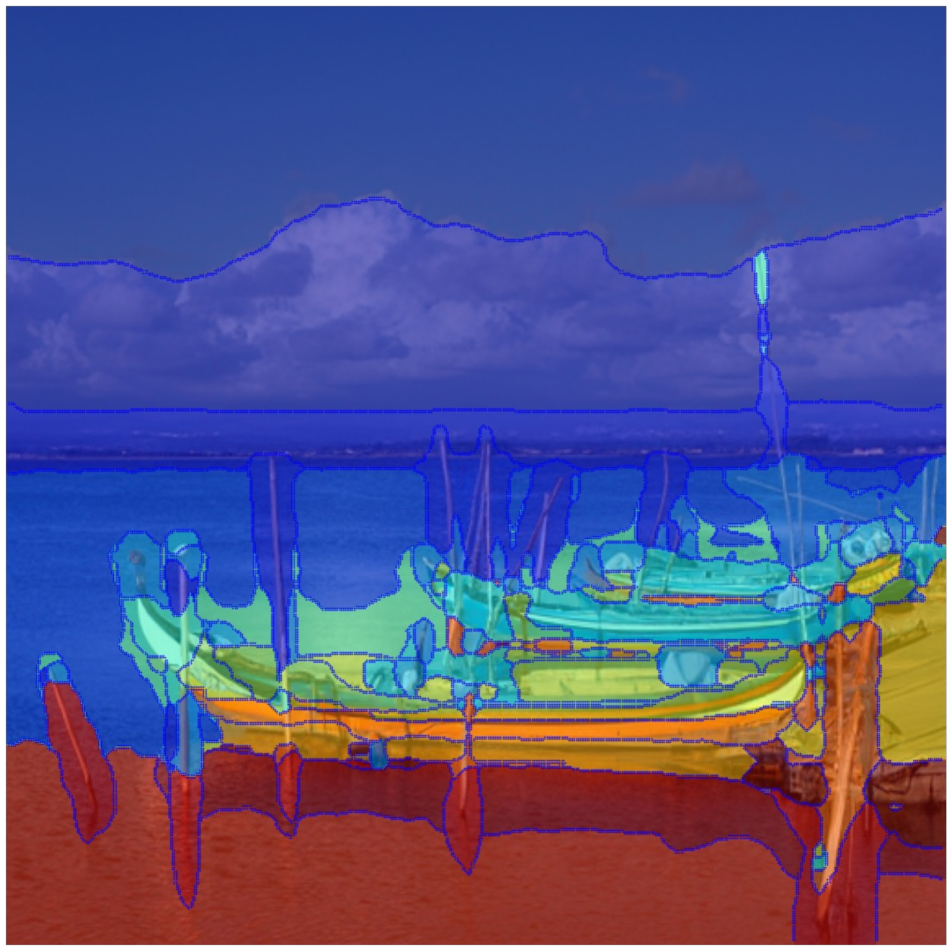
(b) Only $64\times 64$ maps

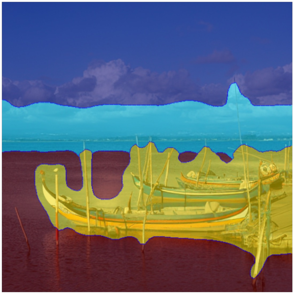
(c) Only $32\times 32$ maps

(d) Only $16(8)\times 16(8)$ maps

(e) Original image

Figure 4: Effects of using Different Aggregation Weights $(R)$. DiffSeg uses a proportional aggregation strategy to balance consistency and detailedness. Higher-resolution maps produce more detailed but fractured segmentation while lower-resolution maps produce more consistent but coarse segmentation.

On the COCO benchmark, we include two k-means baselines, K-Means-C and K-Means-S. K-Means-C uses a constant number of clusters, 6, calculated by averaging over the number of objects in all evaluated images and K-Means-S uses a specific number for each image-based on the number of objects in the ground truth of that image. In Tab. 1, we observe that both K-Means variants outperform prior works, demonstrating the advantage of using self-attention tensors. Furthermore, the K-Means-S variant outperforms the K-Means-C variant. This shows that the number of clusters is an important hyper-parameter and should be tuned for each image. Nevertheless, DiffSeg, even though relying on the same attention tensors $\mathcal{A}_{f}$, significantly outperforms the K-Means baselines. This proves that our algorithm not only avoids the disadvantages of K-Means but also provides better segmentation. Please refer to Appendix 8.4 for more details on the implementation of the K-Means baselines. Moreover, DiffSeg significantly outperforms prior works by an absolute $26\%$ in accuracy and $17\%$ in mIoU compared to the prior SOTA zero-shot method, ReCo on COCO-Stuff-27 for both resolutions (320 and 512).

On the more specialized self-driving segmentation task (Cityscapes), our method is on par with prior works using the smaller 320-resolution input and outperforms prior works using the larger 512-resolution input in both accuracy and mIoU. The resolution of the inputs affects the performance of Cityscapes more severely than of COCO because Cityscapes has more small classes such as light poles and traffic signs. See discussion on limitations in Appendix 8.6. Compared to prior works, DiffSeg achieves this level of performance in a pure zero-shot manner without any language dependency or auxiliary images. Therefore, DiffSeg can segment any image.

4.2 Hyper-Parameter Study

Name	COCO	Cityscapes
Aggregation weights ($R$)	Propto.	Propto.
Time step ($t$)	300	300
Num. of anchors ($M^{2}$)	256	256
Num. of merging iterations ($N$)	3	3
KL threshold ($\tau$)	1.1	0.9

Table 3: Hyper-parameters for Diffseg. The values are used for producing the results in Tab. 1 and Tab. 2.

There are several hyper-parameters in DiffSeg as listed in Tab. 3. The listed numbers are the exact parameters used for Sec. 4.1. In this section, we provide a sensitivity study for these hyper-parameters to illustrate their expected behavior. Specifically, we show the effects of aggregation weights in the main paper and the effects of other hyper-parameters in Appendix 8.5.

Aggregation weights $(R)$. The first step of DiffSeg is attention aggregation, where attention maps of 4 resolutions are aggregated together. We adopt a proportional aggregation scheme. Specifically, the aggregation weight for a map of a certain resolution is proportional to its resolution, i.e., high-resolution maps are assigned higher importance. This is motivated by the observation that high-resolution maps have a smaller receptive field w.r.t the original image thus giving more details. To illustrate this, we show the effects of using attention maps of different resolutions for segmentation in Fig. 4 while keeping other hyper-parameters constant ($t=100,M^{2}=256,N=3,\tau=1.0$). We observe that high-resolution maps, e.g., $64\times 64$ in Fig. 4(b) yield the most detailed however fractured segmentation. Lower-resolution maps, e.g., $32\times 32$ in Fig. 4(c), give more coherent segmentation but often over-segment details, especially along the edges. Finally, too low resolutions fail to generate any segmentation in Fig. 4(d) because the entire image is merged into one object given the current hyper-parameter settings. Notably, our proportional aggregation strategy (Fig. 4(a)) balances consistency and detailedness.

5 Adding Semantics

While DiffSeg generates high-quality segmentation masks, like SAM [20], it does not provide labels for each mask. We propose a simple extension in Appendix 11 to produce labeled segmentation masks.

6 Visualization

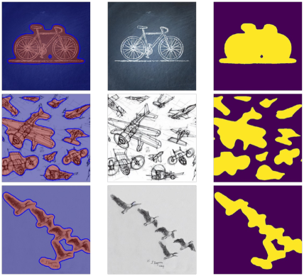
Figure 5: Examples of Segmentation on DomainNet Sketch. Overlay (left), input (middle), and segmentation (right)

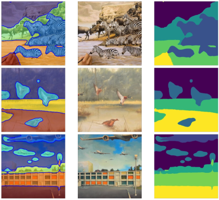
Figure 6: Examples of Segmentation on DomainNet Painting.Overlay (left), input (middle), and segmentation (right)

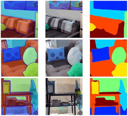
Figure 7: Examples of Segmentation on real-world images captured by a smartphone. Overlay (left), input (middle), and segmentation (right).

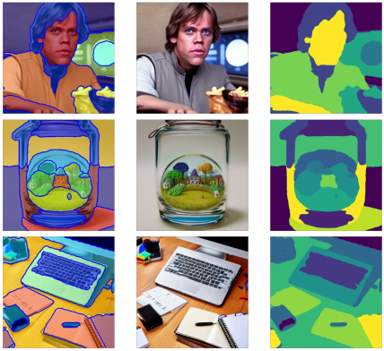
Figure 8: Examples of Segmentation on generated images. Overlay (left), input (middle), and segmentation (right).

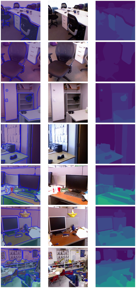
Figure 14: Examples of Segmentation on SUN-RGBD Images. Overlay (left), Input (middle), and segmentation (right)

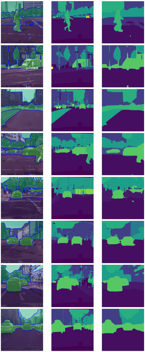
Figure 15: Examples of Segmentation on Cityscapes. Overlay (left), ground truth (middle), and segmentation (right)

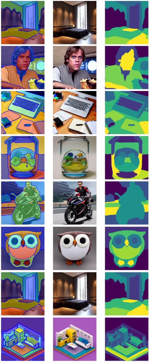
Figure 16: Examples of Segmentation on Synthetic Images (generated by a stable diffusion model). Overlay (left), Input (middle), and segmentation (right)

To demonstrate the generalization capability of DiffSeg, we provide examples of segmentation on images of different styles. In Fig. 5 and Fig. 6, we show segmentation on several sketches and paintings. The images are taken from the DomainNet dataset [31]. In Fig. 7, we show the segmentation results of real images captured by a smartphone. We also provide more segmentation examples Cityscapes in Appendix Fig. 15 and SUN-RGBD [43] in Appendix Fig. 14. Naturally, DiffSeg can segment synthetic images of diverse styles, generated by a stable diffusion model. We show examples in Fig. 8 and more in Appendix Fig. 16.

7 Conclusion

Unsupervised and zero-shot segmentation is a very challenging setting and only a few papers have attempted to solve it. Most of the existing work either requires unsupervised adaptation (not zero-shot) or external resources. In this paper, we proposed DiffSeg to segment an image without any prior knowledge or external resources, using a pre-trained stable diffusion model, without any additional training. Specifically, the algorithm relies on Intra-Attention Similarity and Inter-Attention Similarity to iteratively merge attention maps into a valid segmentation mask. DiffSeg achieves state-of-the-art performance on popular benchmarks and demonstrates superior generalization to images of diverse styles.

8 Appendix

8.1 Stable Diffusion Architecture

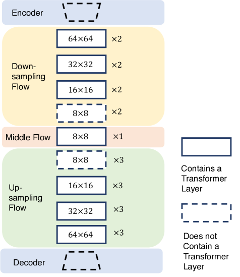
Figure 9: Stable Diffusion Model Schematics. There are in total 16 blocks having Transformer Layers. Each generates a 4D self-attention tensor of different resolutions.

8.2 Discussion on Averaging Multi-head Attentions

In Sec. 3.1, we mentioned that DiffSeg averages the multi-head attention along the multi-head axis, reducing a 5D tensor to 4D. This is motivated by the fact that different attention heads capture very similar correlations. To show this, we calculate the average KL distance across the multi-head axis for all attention tensors of different resolutions used for segmentation. We use 180 training data to calculate the following statistics in Tab. 4.

	COCO	Cityscapes
Avg. multi-heads KL	0.46	0.45
Merge Threshold KL ($\tau$)	1.10	0.90

Table 4: Average KL distance across the multi-head axis and the merge threshold used in the paper.

The difference across the multi-head channels is much smaller than the KL merge threshold used in the paper. This means that the attentions are very similar across the channels and they would have been merged together if not averaged at first because their distance is well below the merge threshold.

8.3 Iterative Attention Aggregation

Algorithm 1 Iterative Attention Merging

$\mathcal{L}_{a},\mathcal{A}_{f},N,\tau\$

$\mathcal{L}_{p}=\left\{\frac{1}{|\mathcal{V}|}\sum_{(i,j)\in\mathcal{V}}\mathcal{A}_{f}[i,j]|v=1,...,M^{2}\right\}$

             where $\mathcal{V}=\{(i,j)|\mathcal{D}\left(\mathcal{L}_{a}[v],\mathcal{A}_{f}[i,j]\right)<\tau\}$

for $N-1$ iterations do

     Initialize $\tilde{\mathcal{L}}_{p}=[]$

     for $\mathcal{A}$ in $\mathcal{L}_{p}$ do

         $V=\frac{1}{|\mathcal{V}|}\sum_{v\in\mathcal{V}}\mathcal{L}_{p}[v]$ $\triangleright$ Merge attention maps

                   where $\mathcal{V}=\{v|\mathcal{D}\left(\mathcal{A},\mathcal{L}_{p}[v]\right)<\tau\}$

         Add $V$ to $\tilde{\mathcal{L}}_{p}$

         Remove $\mathcal{L}_{p}[v]\quad\forall v\in\mathcal{V}\quad$ from $\mathcal{L}_{p}$

     end for

     $\mathcal{L}_{p}\leftarrow\tilde{\mathcal{L}}_{p}$

end for

8.4 Comparisons to K-Means Baselines

DiffSeg uses an iterative merging process to generate the segmentation mask to avoid two major limitations of popular k-means clustering-based algorithms: 1) K-means needs specification of the number of clusters and 2) K-means is stochastic depending on initialization of cluster initialization. In this section, we present a comparison between DiffSeg and a K-means baseline. Specifically, after the Attention Aggregation stage, we obtain a 4D attention tensor $\mathcal{A}_{f}\in\mathbb{R}^{64^{4}}$. Instead of using iterative merging as in DiffSeg, we directly apply the K-means algorithm on tensor $\mathcal{A}_{f}$. To do this, we reshape the tensor to $4096\times 4096$, which represents 4096 vectors of dimension 4096. The goal is to cluster the 4096 vectors into $N$ clusters.

We use the Sklearn k-means implementation [1] with k-means$++$ initialization [4]. We present results for the number of clusters using a constant number averaged over all evaluated images and a specific number for each image. The average number and specific number are obtained from the ground truth segmentation masks. We use the COCO-Stuff dataset as the benchmark.

8.5 Additional Ablation study

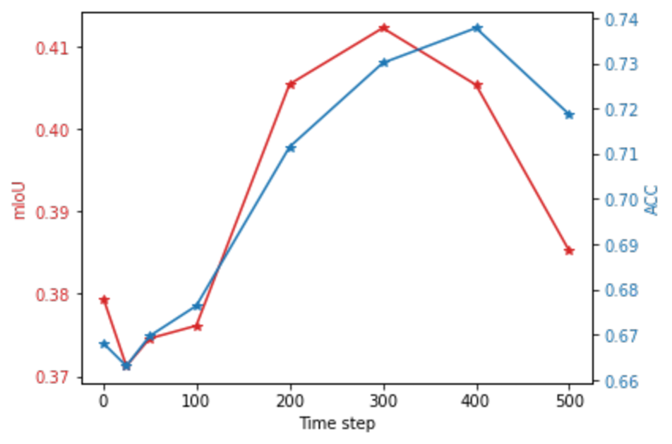
(a) Time Step $t$

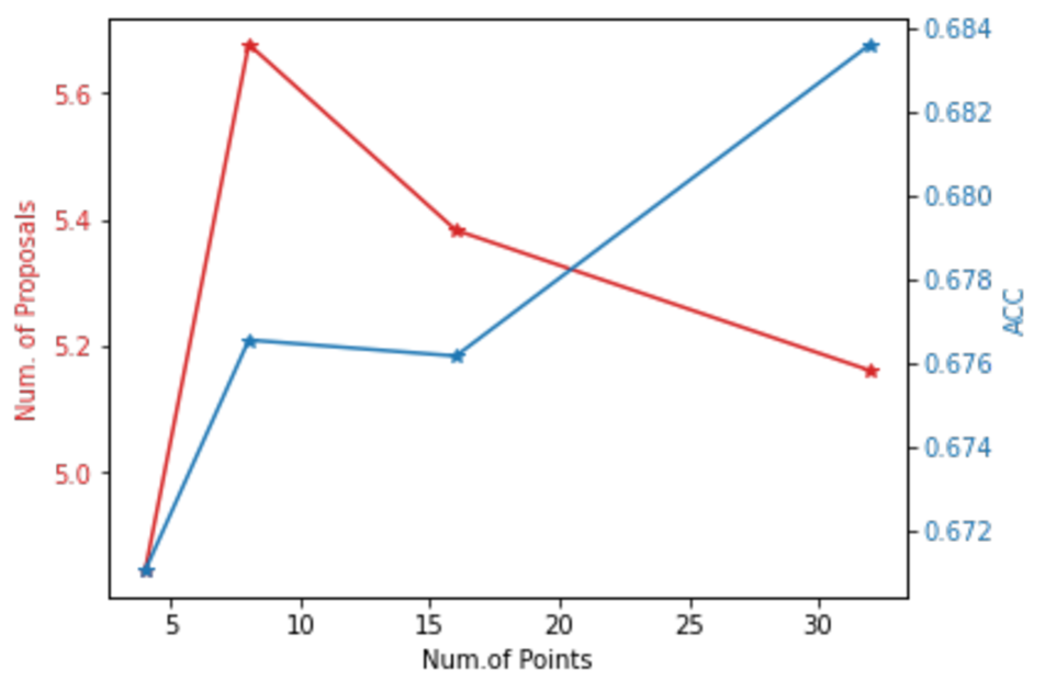
(b) Number of Anchors $M^{2}$

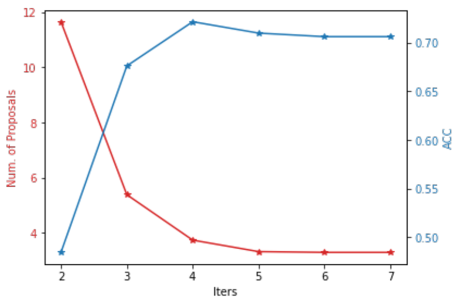
(c) Number of Merging Iters. ($N$)

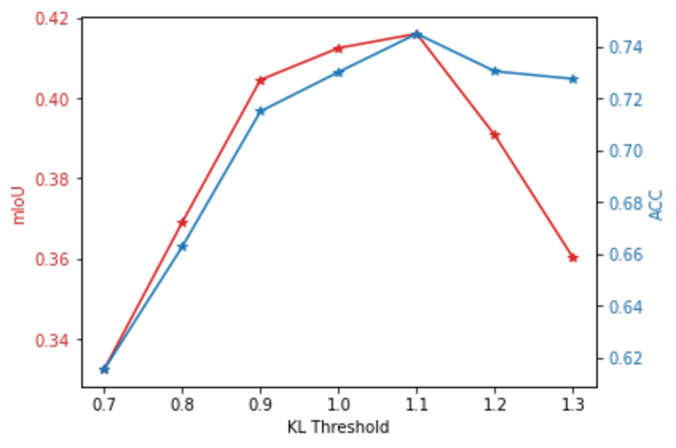
(d) KL threshold $\tau$

Figure 10: Effects of the Time Step $t$, the Number of Anchors $M^{2}$, the Number of Merging Iterations ($N$) and the KL Threshold $\tau$ on COCO-Suff-27. The same set of $(R,t,M,N)$ works generally well for different settings (Tab. 3). A reasonable range for $\tau$ is $0.9\sim 1.1$.

Most of them have a reasonable range that works well for general settings. Therefore, we do not tune them specifically for each dataset and model. One exception is the KL threshold parameter $\tau$. It is the most sensitive parameter as it directly controls the attention-merging process. We tune this parameter in our experiments on a small subset ($180$ images) from the training set from the respective datasets. All sensitivity study experiments are also conducted on the respective subsets.

Time step $(t)$. The stable diffusion model requires a time step $t$ to indicate the current stage of the diffusion process. Because DiffSeg only runs a single pass through the diffusion process, the time step becomes a hyper-parameter. In Fig. 10(a), we demonstrate the effects of setting this parameter to different numbers $t\in\{1,100,200,300,400,500\}$ while keeping the other hyper-parameters constant ($R=\text{propto.},M^{2}=256,N=3,\tau=1.0$). In the figure, we observe a general upward trend for accuracy and mIoU when increasing the time step, which peaked around $t=300$. Therefore, we use $t=300$ for our main results.

Number of anchors $(M^{2})$. DiffSeg generates a sampling grid of $M^{2}$ anchors to start off the attention-merging process. In Fig. 10(b), we show the number of proposals and accuracy with different numbers of anchor points $M\in\{4,8,16,32\}$ while keeping the other hyper-parameters constant ($R=\text{propto.},t=100,N=3,\tau=1.0$). We observe that the number of anchor points does not have a significant effect on the performance of COCO-Stuff-27. Therefore, we keep the default $M=16$.

Number of merging iterations $(N)$. The iterative attention merging process runs for $N$ iterations. Intuitively, the more iterations, the more proposals will be merged. In Fig. 10(c), we show the effects of increasing the number of iterations $N\in\{2,3,4,5,6,7\}$ in terms of the number of final objects and accuracy while keeping the other hyper-parameters constant ($R=\text{propto.},M^{2}=256,t=100,\tau=1.0$). We observe that at the 3rd iteration, the number of proposals drops to a reasonable amount and the accuracy remains similar afterward. Therefore, we use $K=3$ for a better system latency and performance trade-off.

KL threshold $(\tau)$. The iterative attention merging process also requires specifying the KL threshold $\tau$. It is arguably the most sensitive hyper-parameter and should be tuned preferably separately for each dataset. Too small a threshold leads to too many proposals and too large leads to too few proposals. In Fig. 10(d), we show the effect of $\tau\in\{0.7,0.8,0.9,1.0,1.1,1.2,1.3\}$ while using the validated values for the other hyper-parameters ($R=\text{propto.},M^{2}=256,t=100,N=3$). We observe that a range $\tau\in[0.9,1.1]$ should yield reasonable performance. We select $\tau=1.1$ for COCO-Stuff-27 and $\tau=0.9$ for Cityscapes, identified using the same procedure.

A Note on the Hyper-Parameters. We found that the same set of $(R,t,M,N)$ works generally well for different settings. The only more sensitive parameter is $\tau$. A reasonable range for $\tau$ is between 0.9 and 1.1. We would suggest using the default $\tau=1.0$ for the segmentation of images in the wild. For the best benchmark results, proper hyper-parameter selection is preferred.

8.6 Limitations

While the zero-shot capability of DiffSeg enables it to segment almost any image, thanks to the generalization capability of the stable diffusion backbone, its performance on more specialized datasets such as self-driving datasets, e.g., Cityscapes, is far from satisfaction. There are several potential reasons. 1) The resolution of the largest attention map is $64\times 64$, which can be too small to segment small objects in a self-driving dataset. 2) Stable diffusion models have limited exposure to self-driving scenes. The performance of zero-shot methods largely relies on the generalization capability of the pre-trained model. If during the pre-training stage, the stable diffusion model has not been exposed to a vehicle-centric self-driving scene, it could negatively affect the downstream performance. 3) While DiffSeg is much simpler than competing methods such as ReCo [35], which requires image retrieval and co-segmentation of a batch of images, it is still not a real-time algorithm. This is because the current stable diffusion model is very large, even though DiffSeg only runs the diffusion step once. Also, the attention aggregation and merging process are iterative which incurs higher computation costs involving CPU and GPU.

8.7 Adding Semantics

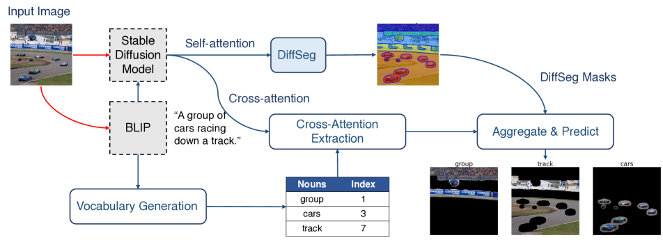
Figure 11: Overview of Semantic DiffSeg. Semantic DiffSeg extends DiffSeg to add labels to generated masks. It has three major additional components Vocabulary Generation, Cross-Attention Extraction and Aggregate $\&$ Predict.

While DiffSeg generates high-quality segmentation masks, like SAM [20], it does not provide labels for each mask. Inspired by recent open-vocabulary semantic segmentation methods [40, 25], which use an off-the-shelf image captioning model to generate vocabularies for an image and DiffuMask [38], which demonstrates the grounding capability of the cross-attention layers in a diffusion model, we propose a simple extension to DiffSeg to produce labeled segmentation masks. We refer to the extended version as Semantic DiffSeg. Specifically, Semantic DiffSeg has three additional components: vocabulary generation, cross-attention extraction, and aggregation $\&$ prediction as shown in Fig. 11.

Vocabulary Generation. Following existing works in open-vocabulary [40, 25] segmentation, we use an off-the-shelf image captioning model, e.g., BLIP [23] to generate a caption for a given image. Denote $\mathcal{W}=\{w_{1},w_{2},...,w_{K}\}$ as the caption where each $w$ represents a word in the caption. To construct the output label space, we extract all nouns from the caption using the NLTK toolkit [28]. Importantly, we also keep track of the relative position of the noun word in the caption for indexing purposes. Formally, let $\mathcal{N}=\{n_{1},n_{2},...n_{L}\}$ denote the set of extracted nouns from $\mathcal{W}$ and $\mathcal{I}=\{i_{1},i_{2},...,i_{L}\}$ denote the set of indices of the relative position corresponding to each noun in the original caption $\mathcal{W}$.

Cross-Attention Extraction. Unlike the vanilla DiffSeg, which uses the unconditional generation capability of stable diffusion models for segmentation without a prompt input, Semantic DiffSeg adds the generated caption $\mathcal{W}$ as another input to extract meaningful grounded cross-attention maps. DiffuMask [38] shows that cross-attention maps corresponding to noun tokens provide grounding for their respective concepts. Inspired by this finding, we also extract the corresponding cross-attention maps from different resolutions using the indices $\mathcal{I}$. Similar to the self-attention formulation in Eq. 1, there are a total 16-cross attention layers in a stable diffusion model, giving 16 cross-attention tensor:

$$\mathcal{A_{C}}\in\{\mathcal{A}_{c}\in\mathbb{R}^{h_{c}\times w_{c}\times Q}|c=1,...,16\}.$$ (7)

where $Q$ is the number of tokenized words in the input caption sequence, e.g., $Q=77$ for stable diffusion models. Unlike the self-attention tensor, the cross-attention tensor is a 3-dimensional tensor, where each $\mathcal{A}_{c}[:,:,q]\in\mathbb{R}^{h_{c}\times w_{c}},\forall q\in\{1,..,Q\}$ is the un-normalized attention map w.r.t the token $q$. We now extract cross-attention maps corresponding to only the nouns in our caption using our index set $\mathcal{I}$. Note that the caption length $K$ is usually smaller than the token sequence length $Q$. Stable diffusion models use BOS and EOS paddings to unify all input lengths to $Q$. Therefore, in our case, the correct index of a noun word w.r.t the padded tokens is its index $i+1$ resulting from the BOS token offset. Finally, we obtain a cross-attention tensor $\mathcal{A_{N}}$ corresponding only to the noun tokens.

$$\mathcal{A_{N}}\in\{\mathcal{A}_{n}\in\mathbb{R}^{h_{n}\times w_{n}\times L}|n=1,...,16\}.$$ (8)

Aggregation and Prediction. Similar to the self-attention maps, the cross-attention maps in $\mathcal{A_{N}}$ are of different resolutions. To aggregate them, we upsample the first 2 dimensions of each map to $512$.

$$\tilde{\mathcal{A}}_{n}=\text{Bilinear-upsample}(\mathcal{A}_{n})\in\mathbb{R}^{512\times 512\times L}.$$ (9)

Note this is slightly different from the upsampling of the self-attention maps in Eq. 10, which upsamples the last 2 dimensions. Finally, we sum and normalize all cross-attention maps to obtain the aggregated cross-attention tensor $\mathcal{A}_{nf}\in\mathbb{R}^{512\times 512\times L}$. Specifically, the aggregated cross-attention map $\mathcal{A}_{nf}^{l}\in\mathbb{R}^{512\times 512}$ corresponding to token $l$ is

$$\mathcal{A}_{nf}^{l}=\frac{\sum_{n=1}^{16}\tilde{\mathcal{A}}_{n}[:,:,l]}{\sum_{w=1}^{512}\sum_{h=1}^{512}\sum_{n=1}^{16}\tilde{\mathcal{A}}_{n}[w,h,l]}.$$ (10)

To obtain the final labeled masks, we combine $\mathcal{A}_{nf}$ with the output from DiffSeg $\bar{\mathcal{L}}_{p}\in\mathbb{R}^{N_{p}\times 512\times 512}$ in Eq. 6, where $N_{p}$ denotes the number of generated masks and each $\bar{\mathcal{L}}_{p}[n_{p},:,:]\in\mathbb{R}^{512\times 512}$ is a binary mask. Specifically, for each mask $\bar{\mathcal{L}}_{p}[n_{p},:,:],n_{p}\in\{1,...,N_{p}\}$, we calculate the prediction vector $l_{n_{p}}\in\mathbb{R}^{L}$. Each element $l_{n_{p}}^{i}$ in $l_{n_{p}}$ is calculated as

$$l_{n_{p}}^{i}=\bar{\mathcal{L}}_{p}[n_{p},:,:]\circledast\mathcal{A}_{nf}[:,:,i],$$ (11)

where $\circledast$ denotes the element-wise product. Finally, the label for mask $n_{p}$ is obtained by taking the maximum element in the prediction vector $l_{n_{p}}$. As a post-processing step, we merge all masks with the same label into a single mask.

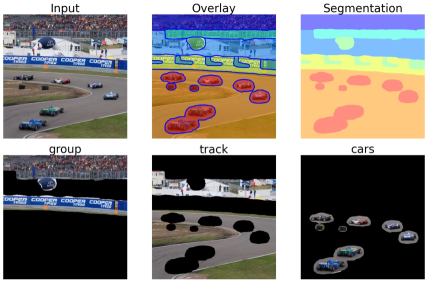
Figure 12: Semantic DiffSeg Example. First row: DiffSeg output. Second row: semantic segmentation with mask merging. Generated caption: A group of cars racing down a track.

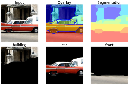
Figure 13: Semantic DiffSeg Example. First row: DiffSeg output. Second row: semantic segmentation with mask merging. Generated caption: A red car parked in front of a building.

8.8 Additional Visualization

References

- [1] Sklearn k-means algorithm. https://scikit-learn.org/stable/modules/generated/sklearn.cluster.KMeans.html.
- [2] Stable diffusion v1-4 model card hugginface. https://huggingface.co/CompVis/stable-diffusion-v1-4.
- [3] Tomer Amit, Tal Shaharbany, Eliya Nachmani, and Lior Wolf. Segdiff: Image segmentation with diffusion probabilistic models. arXiv preprint arXiv:2112.00390, 2021.
- [4] David Arthur and Sergei Vassilvitskii. K-means++ the advantages of careful seeding. In Proceedings of the eighteenth annual ACM-SIAM symposium on Discrete algorithms, pages 1027–1035, 2007.
- [5] Dmitry Baranchuk, Ivan Rubachev, Andrey Voynov, Valentin Khrulkov, and Artem Babenko. Label-efficient semantic segmentation with diffusion models. arXiv preprint arXiv:2112.03126, 2021.
- [6] Maxime Bucher, Tuan-Hung Vu, Matthieu Cord, and Patrick Pérez. Zero-shot semantic segmentation. Advances in Neural Information Processing Systems, 32, 2019.
- [7] Mathilde Caron, Piotr Bojanowski, Armand Joulin, and Matthijs Douze. Deep clustering for unsupervised learning of visual features. In Proceedings of the European conference on computer vision (ECCV), pages 132–149, 2018.
- [8] Mathilde Caron, Hugo Touvron, Ishan Misra, Hervé Jégou, Julien Mairal, Piotr Bojanowski, and Armand Joulin. Emerging properties in self-supervised vision transformers. In Proceedings of the IEEE/CVF international conference on computer vision, pages 9650–9660, 2021.
- [9] Liang-Chieh Chen, George Papandreou, Florian Schroff, and Hartwig Adam. Rethinking atrous convolution for semantic image segmentation. arxiv 2017. arXiv preprint arXiv:1706.05587, 2, 2019.
- [10] Xinlei Chen, Haoqi Fan, Ross Girshick, and Kaiming He. Improved baselines with momentum contrastive learning. arXiv preprint arXiv:2003.04297, 2020.
- [11] Jang Hyun Cho, Utkarsh Mall, Kavita Bala, and Bharath Hariharan. Picie: Unsupervised semantic segmentation using invariance and equivariance in clustering. In Proceedings of the IEEE/CVF Conference on Computer Vision and Pattern Recognition, pages 16794–16804, 2021.
- [12] Marius Cordts, Mohamed Omran, Sebastian Ramos, Timo Rehfeld, Markus Enzweiler, Rodrigo Benenson, Uwe Franke, Stefan Roth, and Bernt Schiele. The cityscapes dataset for semantic urban scene understanding. In Proceedings of the IEEE conference on computer vision and pattern recognition, pages 3213–3223, 2016.
- [13] Di Feng, Christian Haase-Schütz, Lars Rosenbaum, Heinz Hertlein, Claudius Glaeser, Fabian Timm, Werner Wiesbeck, and Klaus Dietmayer. Deep multi-modal object detection and semantic segmentation for autonomous driving: Datasets, methods, and challenges. IEEE Transactions on Intelligent Transportation Systems, 22(3):1341–1360, 2020.
- [14] Qianli Feng, Raghudeep Gadde, Wentong Liao, Eduard Ramon, and Aleix Martinez. Network-free, unsupervised semantic segmentation with synthetic images. In Proceedings of the IEEE/CVF Conference on Computer Vision and Pattern Recognition, pages 23602–23610, 2023.
- [15] Mark Hamilton, Zhoutong Zhang, Bharath Hariharan, Noah Snavely, and William T Freeman. Unsupervised semantic segmentation by distilling feature correspondences. arXiv preprint arXiv:2203.08414, 2022.
- [16] Eric Hedlin, Gopal Sharma, Shweta Mahajan, Hossam Isack, Abhishek Kar, Andrea Tagliasacchi, and Kwang Moo Yi. Unsupervised semantic correspondence using stable diffusion. arXiv preprint arXiv:2305.15581, 2023.
- [17] Jonathan Ho, Ajay Jain, and Pieter Abbeel. Denoising diffusion probabilistic models. Advances in neural information processing systems, 33:6840–6851, 2020.
- [18] Xu Ji, Joao F Henriques, and Andrea Vedaldi. Invariant information clustering for unsupervised image classification and segmentation. In Proceedings of the IEEE/CVF international conference on computer vision, pages 9865–9874, 2019.
- [19] Tero Karras, Samuli Laine, Miika Aittala, Janne Hellsten, Jaakko Lehtinen, and Timo Aila. Analyzing and improving the image quality of stylegan. In Proceedings of the IEEE/CVF conference on computer vision and pattern recognition, pages 8110–8119, 2020.
- [20] Alexander Kirillov, Eric Mintun, Nikhila Ravi, Hanzi Mao, Chloe Rolland, Laura Gustafson, Tete Xiao, Spencer Whitehead, Alexander C Berg, Wan-Yen Lo, et al. Segment anything. arXiv preprint arXiv:2304.02643, 2023.
- [21] Harold W Kuhn. The hungarian method for the assignment problem. Naval research logistics quarterly, 2(1-2):83–97, 1955.
- [22] Alexander C Li, Mihir Prabhudesai, Shivam Duggal, Ellis Brown, and Deepak Pathak. Your diffusion model is secretly a zero-shot classifier. arXiv preprint arXiv:2303.16203, 2023.
- [23] Junnan Li, Dongxu Li, Caiming Xiong, and Steven Hoi. Blip: Bootstrapping language-image pre-training for unified vision-language understanding and generation. In International Conference on Machine Learning, pages 12888–12900. PMLR, 2022.
- [24] Kehan Li, Zhennan Wang, Zesen Cheng, Runyi Yu, Yian Zhao, Guoli Song, Chang Liu, Li Yuan, and Jie Chen. Acseg: Adaptive conceptualization for unsupervised semantic segmentation. In Proceedings of the IEEE/CVF Conference on Computer Vision and Pattern Recognition, pages 7162–7172, 2023.
- [25] Feng Liang, Bichen Wu, Xiaoliang Dai, Kunpeng Li, Yinan Zhao, Hang Zhang, Peizhao Zhang, Peter Vajda, and Diana Marculescu. Open-vocabulary semantic segmentation with mask-adapted clip. In Proceedings of the IEEE/CVF Conference on Computer Vision and Pattern Recognition, pages 7061–7070, 2023.
- [26] Huan Ling, Karsten Kreis, Daiqing Li, Seung Wook Kim, Antonio Torralba, and Sanja Fidler. Editgan: High-precision semantic image editing. Advances in Neural Information Processing Systems, 34:16331–16345, 2021.
- [27] Xiangbin Liu, Liping Song, Shuai Liu, and Yudong Zhang. A review of deep-learning-based medical image segmentation methods. Sustainability, 13(3):1224, 2021.
- [28] Edward Loper and Steven Bird. Nltk: The natural language toolkit. arXiv preprint cs/0205028, 2002.
- [29] Timo Lüddecke and Alexander Ecker. Image segmentation using text and image prompts. In Proceedings of the IEEE/CVF Conference on Computer Vision and Pattern Recognition, pages 7086–7096, 2022.
- [30] Tam Nguyen, Maximilian Dax, Chaithanya Kumar Mummadi, Nhung Ngo, Thi Hoai Phuong Nguyen, Zhongyu Lou, and Thomas Brox. Deepusps: Deep robust unsupervised saliency prediction via self-supervision. Advances in Neural Information Processing Systems, 32, 2019.
- [31] Xingchao Peng, Qinxun Bai, Xide Xia, Zijun Huang, Kate Saenko, and Bo Wang. Moment matching for multi-source domain adaptation. In Proceedings of the IEEE International Conference on Computer Vision, pages 1406–1415, 2019.
- [32] Alec Radford, Jong Wook Kim, Chris Hallacy, Aditya Ramesh, Gabriel Goh, Sandhini Agarwal, Girish Sastry, Amanda Askell, Pamela Mishkin, Jack Clark, et al. Learning transferable visual models from natural language supervision. In International conference on machine learning, pages 8748–8763. PMLR, 2021.
- [33] Robin Rombach, Andreas Blattmann, Dominik Lorenz, Patrick Esser, and Björn Ommer. High-resolution image synthesis with latent diffusion models. In Proceedings of the IEEE/CVF conference on computer vision and pattern recognition, pages 10684–10695, 2022.
- [34] Chitwan Saharia, William Chan, Saurabh Saxena, Lala Li, Jay Whang, Emily L Denton, Kamyar Ghasemipour, Raphael Gontijo Lopes, Burcu Karagol Ayan, Tim Salimans, et al. Photorealistic text-to-image diffusion models with deep language understanding. Advances in Neural Information Processing Systems, 35:36479–36494, 2022.
- [35] Gyungin Shin, Weidi Xie, and Samuel Albanie. Reco: Retrieve and co-segment for zero-shot transfer. Advances in Neural Information Processing Systems, 35:33754–33767, 2022.
- [36] Gyungin Shin, Weidi Xie, and Samuel Albanie. Namedmask: Distilling segmenters from complementary foundation models. In Proceedings of the IEEE/CVF Conference on Computer Vision and Pattern Recognition, pages 4960–4969, 2023.
- [37] Huiyu Wang, Yukun Zhu, Hartwig Adam, Alan Yuille, and Liang-Chieh Chen. Max-deeplab: End-to-end panoptic segmentation with mask transformers. In Proceedings of the IEEE/CVF conference on computer vision and pattern recognition, pages 5463–5474, 2021.
- [38] Weijia Wu, Yuzhong Zhao, Mike Zheng Shou, Hong Zhou, and Chunhua Shen. Diffumask: Synthesizing images with pixel-level annotations for semantic segmentation using diffusion models. arXiv preprint arXiv:2303.11681, 2023.
- [39] Enze Xie, Wenhai Wang, Zhiding Yu, Anima Anandkumar, Jose M Alvarez, and Ping Luo. Segformer: Simple and efficient design for semantic segmentation with transformers. Advances in Neural Information Processing Systems, 34:12077–12090, 2021.
- [40] Jiarui Xu, Sifei Liu, Arash Vahdat, Wonmin Byeon, Xiaolong Wang, and Shalini De Mello. Open-vocabulary panoptic segmentation with text-to-image diffusion models. In Proceedings of the IEEE/CVF Conference on Computer Vision and Pattern Recognition, pages 2955–2966, 2023.
- [41] Andrii Zadaianchuk, Matthaeus Kleindessner, Yi Zhu, Francesco Locatello, and Thomas Brox. Unsupervised semantic segmentation with self-supervised object-centric representations. arXiv preprint arXiv:2207.05027, 2022.
- [42] Junyi Zhang, Charles Herrmann, Junhwa Hur, Luisa Polania Cabrera, Varun Jampani, Deqing Sun, and Ming-Hsuan Yang. A tale of two features: Stable diffusion complements dino for zero-shot semantic correspondence. arXiv preprint arXiv:2305.15347, 2023.
- [43] Bolei Zhou, Agata Lapedriza, Jianxiong Xiao, Antonio Torralba, and Aude Oliva. Learning deep features for scene recognition using places database. Advances in neural information processing systems, 27, 2014.
- [44] Chong Zhou, Chen Change Loy, and Bo Dai. Extract free dense labels from clip. In European Conference on Computer Vision, pages 696–712. Springer, 2022.