Combinatorial insight of Riemann Boundary value problem in lattice walk problems

Abstract

Enumeration of quarter-plane lattice walks with small steps is a classical problem in combinatorics. An effective approach is the kernel method and the solution is derived by positive term extraction. Another approach is to reduce the lattice walk problem to a Carleman type Riemann boundary value problem (RBVP) and solve it by complex analysis. There are two parameter characterizing the solutions of a Carleman type Riemann Boundary value problem, the index $\chi$ and the conformal gluing function $w(x)$. In this paper, we propose a combinatorial insight to the RBVP approach. We show that the index can be treated as the canonical factorization in the kernel method and the conformal gluing function can be turned into a conformal mapping such that after this mapping, the positive degree terms and the negative degree terms can be naturally separated. The combinatorial insight of RBVP provide a connection between the kernel method, the RBVP approach and the Tutte’s invariant method.

1 Introduction

Quarter-plane lattice walks refer to walks with fixed step sets (allowed lengths and directions), ending on the grid and restricted in the quarter. By solving a lattice walk problem, we mean finding an explicit expression of the number of configurations of $n$-step walks ending on an arbitrary vertex or the generating function of this number of configurations. Enumeration of lattice walks is a classical combinatorial problem and it has close relations with probability[30], mathphysics[16], integral systems[44] and representation theory[36]. Quarter-plane lattice walks with small steps are well studied in the past several years. In [13], Bousquet-Mélou and Mishna distinguished all $256$ possible walks into $79$ different non-trivial two-dimensional models. Among these $79$ models, there are $23$ associated with finite symmetry groups. These models can further be classified: $16$ models are associated with $D_{2}$ groups, five models with $D_{3}$ groups and two models with $D_{4}$ groups.

There are several different approaches to lattice walk problems. In [13] and [11], Bousquet-Mélou and Mishna introduced the kernel method appraoch and solve all the models associated with finite groups. In [32], Stephen Melczer and Marni Mishna use iterate kernel method to prove formulas for asymptotic behaviors and find an explicit expression for the generating functions of some singular models.

Before combinatoricists got interested in quarter-plane lattice walk problems, probabilists had developed an analytic approach to quarter-plane random walks. In [30], V.A.Malyshev reduced the lattice walk problem to a Riemann Boundary value problem (RBVP) with Carleman shift[29] and solve it via comformal mapping. This approach was generalized and extended to enumeration of lattice walks in [38].

There are also many other works about quarter plane lattice walk problems [7, 21, 10, 25, 33, 39, 39, 20, 27] and the methods range from combinatorics, probability theory, algebraic geometry, complex analysis and computer algebra.

2 Motivation

All the method are interesting and powerful. A very mysterious thing is that every approach has a different solution form. But it is not obvious that these solutions are equivalent. For example, if we consider solving the simple lattice walk (walk with allow steps $\{\uparrow,\downarrow,\leftarrow,\rightarrow\}$, starting form the origin $(0,0)$) restricted in the quarter-plane via bijections and inclusion-exclusion, the solution reads [24],

$$|P^{++}_{n}((0,0)\to(i,j))|=\binom{n}{\frac{n+i-j}{2}}\binom{n+2}{\frac{n-i-j}{2}}-\binom{n+2}{\frac{n+i-j}{2}+1}\binom{n}{\frac{n-i-j}{2}-1},$$ (2.1)

where $|P^{++}_{n}((0,0)\to(i,j))|$ refers to the number of $n$-step walks starting from $(0,0)$, ending at $(i,j)$.

If we solve it via the algebraic kernel method [10], the solution has an extremely simple form,

$$Q(x,y,t)=[x^{>}y^{>}]\frac{xy-x/y-y/x+1/x/y}{K(x,y)}.$$ (2.2)

$Q(x,y,t)$ (normally abbreviated as $Q(x,y)$) is the generating function,

$$Q(x,y)=\sum_{i,j,k}q_{ijn}x^{i}y^{j}t^{n},$$ (2.3)

where $q_{ijn}$ refers to the number of $n$-step paths starting from the origin, ending at $(i,j)$ and $i,j,n\geq 0$. In algebraic combinatorics, we regularly use $[x^{i}]f(x)$ to denote the coefficient of $i$th degree term of $x$ in $f(x)$. We use $[x^{>}]f(x)$ to denote the positive degree terms of $x$ in $f(x)$. $K(x,y)$ is called the kernel of the lattice walk, it is

$$K(x,y)=1-t(x+1/x+y+1/y).$$ (2.4)

Another approach in algebraic combinatorics is the obstinate kernel method. This method is introduced in [37] and has been widely applied in different lattice walk problems [2]. Instead of solving $Q(x,y)$ directly, the obstinate kernel method solve the boundary value $Q(x,0)$ and $Q(0,y)$ first. The solution reads,

$$Q(x,0)=\frac{1}{tx}[x^{>}]Y_{0}(x)(x-1/x).$$ (2.5)

Where $Y_{0}(x),Y_{1}(x)$ are roots of $K(x,Y)=0$. And $Y_{0}(x,t)$ should be considered as a formal series of $t$. We can see that the solution form in both kernel method approaches involve the positive degree term extraction (taking $[x^{>}]$). This is a technique widely used in solving discrete differential equations [18].

It is straight forward to get the solutions form of bijections and inclusion-exclusion from the algebraic kernel method. For simple lattice walk, $|P^{++}_{n}((0,0)\to(i,j))|=q_{i,j,m}=[x^{i}y^{j}t^{n}]Q(x,y,t)$ in (2.2). We need to do some careful calculations with binomial expansion.

The transform between the form of algebraic kernel method and the obstinate kernel method follows the fact,

$$\frac{1}{K(x,y)}=\frac{1}{t(Y_{0}-Y_{1})}\left(\sum_{i\geq 0}\left(\frac{Y_{0}(x)}{y}\right)^{i}+\sum_{i\geq 0}\left(\frac{y}{Y_{1}(x)}\right)^{i}-1\right).$$ (2.6)

$Y_{0}(x)$ and $Y_{1}(x)$ are two roots of $K(x,y)=0$. Taking $[x^{>}]$ gives,

$$[x^{>}]f(x,Y_{0}(x))=[x^{>}]f(x,y)-[x^{>}]\Big{(}K(x,y)[y^{>}]\frac{f(x,y)-f(x,1/y)}{K(x,y)}\Big{)},$$ (2.7)

where $f(x,y)$ is a polynomial in $x,y$. One can also calculate the explicit number of configurations via the techniques used in [3], a wonderful application of Lagrange-Bürmann inversion formula.

Different from the combinatotrial idea, the RBVP approach gives a solution in integral form. It generally looks like

$$c(x,t)Q(x,0,t)=\frac{1}{2\pi i}\oint_{X_{0}[y_{1},y_{2}]}sY_{0}\frac{\partial_{s}w(s,t)}{w(s,t)-w(x,t)}ds+c(0,t)Q(0,0,t),$$ (2.8)

$c(x,t)$ is some known coefficient. $X_{0}[y_{1},y_{2}]$ is a contour on $x$-plane. $X_{0}(y)$ is the roots of the kernel $K(X,y)=0$. If we write $X_{0}(y)=\frac{-b(y)-\sqrt{\Delta(y)}}{2a(y)}$, $y_{1},y_{2}$ are the two small roots of $\Delta(y)$. $w(x,t)$ is an conformal mapping with additional gluing properties, called conformal gluing function. It is originally expressed as an Weistrass $\wp$ function in [21] and later obtains a algebraic expression for models associated with finite groups [38]. The approach to this integral form follows a standard process to Riemann boundary value problem with Carleman shift [29]. The problem is defined as follow:

Definition 1.

Find a function $\Phi^{+}$ holomorphic in some domain $L^{+}$, the limiting value of which on the closed contour $L$ are continuous and satisfies the equation,

$$\Phi^{+}(\alpha(s))=G(s)\Phi^{+}(s)+g(s),\qquad s\in L,$$ (2.9)

where

1. For any $s\in L$, $g$ and $G$ are Hölder continuous on $L$ and $G(s)\neq 0$.

2. The function $\alpha(s)$ is an one-one mapping of $L\to L$ such that $\alpha(\alpha(s))=s$ and $\alpha$ is Hölder continuous.

A function $f$ is said to be Hölder continuous [35] if for any two points $s_{1},s_{2}$ on $L$, we can find positive constants $A$ and $\mu$, such that,

$$|f(s_{1})-f(s_{2})|\leq A|s_{1}-s_{2}|^{\mu}.$$ (2.10)

It is proved [29] that there exists a function $z=w(x)$, which is holomorphic in $L^{+}$ except one point $z_{0}$ and satisfying the following gluing property,

$$w(\alpha(s))-w(s)=0\qquad s\in L.$$ (2.11)

It is a conformal mapping from the domain $L^{+}$ in $x$-plane onto the complex $z$-plane with cut $[ab]$. The inverse mapping is denoted as $x=w^{-1}(z)$.

Let $\chi=-\frac{[argG(w^{-1}(z^{-}))]_{[ab]}}{2\pi}$. $\chi$ is called the index of this problem. If $\chi=-1$, a general solution reads,

$$\Phi^{+}(x)=\frac{X(w(x))}{2\pi i}\oint_{\lfloor ab\rfloor}\frac{g(w^{-1}(s^{-}))}{X^{+}(s)(s-w(x))}ds=-\frac{X(w(x))}{2\pi i}\oint_{L_{d}}\frac{\partial_{s}w(u)g(u)}{X^{+}(w(u))(w(u)-w(x))}du,$$ (2.12)

where

$$\begin{cases}&\Gamma(z)=\frac{1}{2\pi i}\int_{\lfloor ab\rfloor}\frac{log(G(w^{-1}(s)))}{s-z}ds\\ &X(z)=(z-b)^{-\chi}e^{\Gamma(z)}.\end{cases}$$ (2.13)

$\lfloor ab\rfloor$ is taken as the lower part of cut $[ab]$ and $L_{d}$ is the lower part of $L$. If $\chi\leq-1$, $-\chi-1$ extra condition is needed,

$$\frac{1}{2\pi i}\int_{\lfloor ab\rfloor}\frac{g(w^{-1}(s))}{X^{+}(s)s^{k-1}}ds\qquad k=1,2,\dots-\chi-1.$$ (2.14)

If $\chi\geq 0$, then (2.9) has $1+\chi$ linearly independent solutions reads,

$$\Phi^{+}(z)=\frac{X(w(z))}{2\pi i}\oint_{[ab]}\frac{g(w^{-1}(s^{-}))}{X^{+}(s)(s-w(z))}ds+X(w(z))P_{\chi}(z).$$ (2.15)

where $P_{\chi}(z)$ is a polynomial of degree $\chi$. This $\chi$ can be understood as the degree of singularity near the end point. If we consider $z$ near the end point $c$ of the contour ($c$ can be either $a$ or $b$).

$$\Gamma(z)=\epsilon_{c}\frac{logG(c)}{2\pi i}log(z-c)+\gamma_{c}(z),$$ (2.16)

where $\epsilon_{c}=1$ for the start point $c=a$ and $\epsilon_{c}=-1$ for the end point $c=b$. Further,

$$logG(c)=log|G(c)|+iargG(c).$$ (2.17)

If we let the argument of $G$ be $0$ at start point $a$, then $\Gamma(z)$ has a singularity of $\frac{argG(b)}{2\pi}log(z-b)$ at the end point $b$. Then $X(z)=(z-b)^{-\chi}e^{\Gamma(z)}$ is an analytic function near both end point of the branch cut $[ab]$.

(2.8) is just the simple case with $G(z)=1$ and $\chi=0$. But for three-quarter walks [40] or weighted walks [21], it is not $0$ in general.

Here is a natural question. Does (2.8) for simple lattice walk equals to (2.5)? They are solutions in different representations but it is not easy to transform one to the other. Also, we introduced two functions, $\chi$ and $w(z)$ in the RBVP solution. $\chi$ characterize the number of linear independent solution and $w(z)$ characterize the integral. Is there any combinatorial correspondence to these two functions in the kernel method approach? These two functions play important roles in RBVP, but from all the current results people got via the kernel method approach[34, 10, 5, 6, 11], they are hidden.

Let us somehow recall the functional equation in obstinate kernel method a bit. Taking simple lattice walk as an example. During the calculation, we meet an equation,

$$Y_{0}(x)\left(x-\frac{1}{x}\right)=txQ(x,0)-\frac{t}{x}Q\left(\frac{1}{x},0\right)$$ (2.18)

Since $txQ(x,0)$ is defined as a formal series of $x$ and $t/xQ(1/x,0)$ is a formal series of $1/x$, we take the $[x^{>}]$ of (2.18) and (2.5) follows immediately. Comparing (2.18) and (2.9), if we write $\alpha(x)=1/x$, (2.18) looks similar to a boundary value problem. Although $x$ defined in (2.18) is a parameter in the generating functions and $s$ in (2.9) is some point on a curve $L$ on $x$-plane, there is still a strong intuition that $\chi$ and $w(x)$ shall have their position in the kernel method approach.

To show where and how $\chi$ emerges in the obstinate kernel method, we will make the problem a bit complicate. we consider quarter-plane lattice walk with boundary interactions. It is some supplement work to [6, 5, 45] and there are still some models unsolved. We will show that the combinatorial correspondence of $\chi$ characterize the solvability of some models with interactions.

To show where and how $w(z)$ emerges in the obstinate kernel method, we will compare the combinatorial and analytic insight of lattice walk problems, and find a combinatorial version of the conformal gluing function.

3 Organization of this paper

The paper will be separated into two parts. In the first part, namely, Section 5 to Section 11 we consider quarter-plane lattice walk with boundary interactions. We show the canonical factorization introduced in [23] can be treated as a combinatorial version of index $\chi$.

In the second part, namely, Section 13 to Section 15, we consider quarter-plane lattice walk without boundary interactions for simplicity. We introduce a combinatorial conformal mapping and show that it connects the results in combinatorial approach and RBVP approach.

4 Definition and Notations for Lattice walk with interactions

4.1 Notations for Algebra

Suppose $f(x)$ is a series of both $x$ and $1/x$. We write $[x^{i}]f(x)$ as the coefficient of $i$th degree term of $x$ in $f(x)$. $[x^{>}]f(x)$, $[x^{<}]f(x)$ and $[x^{\geq}]f(x)$ are those terms of positive, negative and non-negative degree terms of $x$ in $f(x)$.

For a ring or a field $\mathbb{K}$, we denote

1. $\mathbb{K}[t]$ as the set of polynomials in $t$ with coefficients in $\mathbb{K}$;

2. $\mathbb{K}[t,\frac{1}{t}]$ as the set of polynomials in $t$ and $\frac{1}{t}$ with coefficients in $\mathbb{K}$.

3. $\mathbb{K}[[t]]$ as the set of formal power series in $t$ with coefficients in $\mathbb{K}$;

4. $\mathbb{K}((t))$ as the set of Laurent series in $t$ with coefficients in $\mathbb{K}$;

5. $\mathbb{K}(t)$ as the set of rational functions in $t$ with coefficients in $\mathbb{K}$.

The notations extend to multiple variables. For example $\mathbb{R}((x))((t))$ refers to the set of Laurent series in $t$ with coefficients in the set of formal power series of $x$ with real coefficients. Also notice that multivariate Larent expansion are defined iteratedly [31] and $\mathbb{R}((x))((t))\neq\mathbb{R}((t))((x))$.

We consider the following set of functions,

1. Algebraic: $f(x)$ is algebraic over $x$ if there exists a polynomial equation $P(f,x)=0$ with coefficients in $\mathbb{C}(x)$.

2. D-finite: $f(x)$ is D-finite (short for differentiably finite, also called holonomic) over $x$ if there exists a linear equation $L(f,f^{\prime},\dots f^{(n)})=0$ with coefficients in $\mathbb{C}(x)$.

3. D-algebraic: $f(x)$ is D-algebraic (differentiably algebraic, also called hyper-algebraic) over $x$ if there exists a polynomial equation $P(f,f^{\prime},\dots f^{(n)})=0$ with coefficients in $\mathbb{C}(x)$.

4. Hyper-transcendental $f(x)$ does not satisfy any of the previous three conditions.

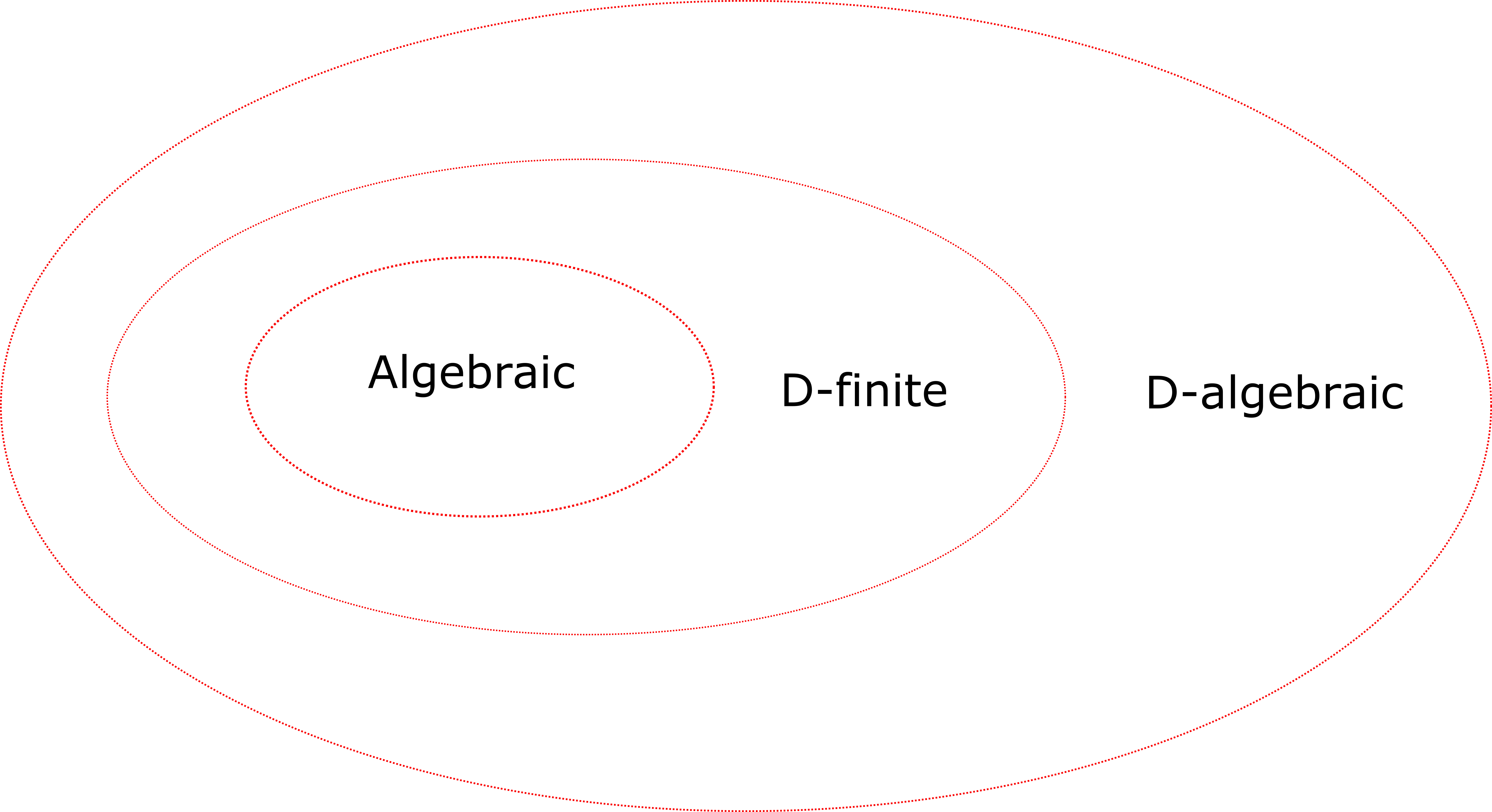
Figure 1: The relation between algebraic, D-finite and D-algebraic

In multivariate cases, $f(x_{1},x_{2}\dots x_{k})$ is said to be D-finite (algebraic, D-algebraic) if there exist $k$ linear (polynomial) equations $L_{i}(f,\frac{\partial f}{\partial x_{i}},\dots\frac{\partial^{n}f}{\partial x_{i}^{n}})=0$, $(i=1,2,\dots k)$ with coefficients in $\mathbb{C}(x_{1},x_{2}\dots,x_{n})$ [28]. We may also specify D-finite (algebraic, D-algebraic) over $x_{i}$ if they satisfy the corresponding one-variable condition for $x_{i}$.

The set of algebraic functions and the set of D-algebraic functions are fields [1] and they are closed under addition, multiplication and inversion. The set of D-finite functions is closed under addition and multiplication. But the inverse $1/f$ of a D-finite function $f$ is not necessarily D-finite. See [42, 1] for more properties of these sets of functions.

Definition 2.

Given two series $f(x)=\sum_{i}f_{i}x^{i}$ and $g(x)=\sum_{i}g_{i}x^{i}$. The Hadamard product $f*g$ is defined as

$$f(x)*g(x)=\sum_{i}f_{i}g_{i}x^{i}.$$ (4.1)

Hadamard product is strongly related to the operations $[x^{0}],[x^{>}],[x^{<}]$ by the following equations,

$$f(x)*g(x)=[u^{0}]f(x/u)g(u)$$ (4.2)

$$[x^{\geq}]f(x)=[u^{0}]\frac{f(x/u)}{1-u}.$$ (4.3)

4.2 Notations for lattice walk models

We denote $q_{n,k,l,h,v,u}$ as the number of paths of length $n$ that start at $(0,0)$, end at $(k,l)$, and visit vertices on the horizontal boundary (except the origin) $h$ times, on the vertical boundary (except the origin) $v$ times and the origin $u$ times. The generating function is

$$Q(x,y,t;a,b,c)\equiv Q(x,y)=\sum_{n}t^{n}\sum_{k,l,h,v,u}q_{n,k,l,h,v,u}x^{k}y^{l}a^{h}b^{v}c^{u} \equiv\sum_{n}t^{n}Q_{n}(x,y)$$

$$\equiv\sum_{i,j}Q_{i,j}x^{i}y^{j}.$$ (4.4)

For convenience, we always omit $t$ in the notations.

We define line-boundary terms:

$$[y^{i}]Q(x,y,t;a,b,c)\equiv Q_{-,i}(x)=\sum_{n}t^{n}\sum_{k,h,v,u}q_{n,k,i,h,v,u}x^{k}a^{h}b^{v}c^{u}.$$ (4.5)

This is the generating function of walks ending on the line $y=i$. $Q_{i,-}(y)$ is defined similarly. For walks ending on the line $y=0$ ($x=0$), we prefer a more convenient expression $Q(x,0)$ or $Q(0,y)$.

For walks without interactions, just set $a,b,c$ equals $1$ and we get the corresponding $Q(0,y)$, $Q(x,0)$ and $Q(x,y)$.

4.3 Derivation of the functional equation

Consider a walk starting from the origin with allowed steps $\mathcal{S}\subseteq\{-1,0,1\}\times\{-1,0,1\}\setminus\{0\}\times\{0\}$. The step generator $S$ is

$$S(x,y)=\sum_{(i,j)\in\mathcal{S}}x^{i}y^{j}.$$ (4.6)

It can be written as

$$S(x,y)=A_{-1}(x)\frac{1}{y}+A_{0}(x)+A_{1}(x)y=B_{-1}(y)\frac{1}{x}+B_{0}(y)+B_{1}(y)x$$ (4.7)

$|S|$ refers to the number of allowed steps.

Theorem 3.

[45] For a lattice walk restricted to the quarter-plane, starting from the origin, with weight ‘$a$’ associated with steps ending on the $x$-axis (except the origin), weight ‘$b$’ associated with steps ending on $y$-axis (except the origin) and weight ‘$c$’ associated with steps ending at the origin, the generating function $Q(x,y)$ satisfies the following functional equation:

$$K(x,y)Q(x,y)=\frac{1}{c}+\frac{1}{a}\Big{(}a-1-taA_{-1}(x)\frac{1}{y}\Big{)}Q(x,0)+\frac{1}{b}\Big{(}b-1-tbB_{-1}(y)\frac{1}{x}\Big{)}Q(0,y)\\ +\left(\frac{1}{abc}(ac+bc-ab-abc)+\frac{t[x^{-1}y^{-1}]S(x,y)}{xy}\right)Q(0,0)$$ (4.8)

where $K(x,y)=1-tS(x,y)$. $K(x,y)$ is called the kernel of the walk.

Proof.

We give a simple proof here. Consider how one obtains the configuration by adding a single step onto a walk of arbitrary length. For a walk in the quarter-plane with boundary interactions, we have $7$ situations,

1. The empty walk with no steps. This gives $1$.

2. Walks ending away from the boundary, which gives

   $$tS(x,y)\big{(}Q(x,y)-Q_{-,1}(x)-Q_{1,-}(y)-Q_{-,0}(x)-Q_{0,-}(y)+Q_{1,1}+Q_{0,0}+Q_{0,1}+Q_{1,0}\big{)}$$

   $$+t([x^{>}]S(x,y))\big{(}Q_{0,-}(y)-Q_{0,0}-Q_{0,1}\big{)}+t([x^{\geq}]S(x,y))\big{(}Q_{1,-}(y)-Q_{1,1}-Q_{1,0}\big{)}$$

   $$+t([y^{>}]S(x,y))\big{(}Q_{-,0}(x)-Q_{0,0}-Q_{1,0}\big{)}+t([y^{\geq}]S(x,y))\big{(}Q_{-,1}(x)-Q_{1,1}-Q_{1,0}\big{)}$$

   $$+t[x^{>}y^{>}]S(x,y)Q_{0,0}+t[x^{\geq}y^{\geq}]S(x,y)Q_{1,1}.$$

   We need to subtract the steps that interact with boundary and those steps that go outside the quarter-plane (We call these steps “illegal” steps).

3. Walks arriving at the positive $x$-axis, which gives

   $$at\left(\frac{1}{y}A_{-1}(x)(Q_{-,1}(x)-Q_{0,1})-\frac{[x^{-1}y^{-1}]S(x,y)}{xy}Q_{1,1}+\frac{1}{y}[x^{1}]A_{-1}(x)Q_{0,1}\right)$$

4. Walks along the positive $x$-axis, which gives

   $$at\left([y^{0}]S(x,y)(Q_{-,0}(x)-Q_{1,0}-Q_{0,0})+[x^{1}y^{0}]S(x,y)(Q_{1,0}+Q_{0,0})\right)$$

5. Walks arriving at the positive $y$-axis, which gives

   $$bt\left(\frac{1}{x}B_{-1}(y)(Q_{1,-}(y)-Q_{1,0})-\frac{[x^{-1}y^{-1}]S(x,y)}{xy}Q_{1,1}+\frac{1}{x}[y^{1}]B_{-1}(y)Q_{0,1}\right)$$

6. Walks along the positive $y$-axis, which gives

   $$bt\left([x^{0}]S(x,y)(Q_{0,-}(y)-Q_{0,1}-Q_{0,0})+[x^{0}y^{1}]S(x,y)(Q_{0,1}+Q_{0,0})\right)$$

7. Walks ending at the origin, which gives

   $$ct\left(\frac{[x^{-1}y^{-1}]S(x,y)}{xy}Q_{1,1}+[x^{-1}y^{0}]S(x,y)Q_{1,0}+[x^{0}y^{-1}]S(x,y)Q_{0,1}\right)$$

Summing cases (i)– (vii) together, we get $Q(x,y)$. We have many unknowns, $Q_{-,1}(x)$, $Q_{0,0}$, $Q_{1,1}$ etc. Notice that case  (i)+(iii)+(iv)+(vii)  actually equals $Q(x,0)$ and case  (i)+(v)+(vi)+(vii)  equals $Q(0,y)$ by definition. This provides a way to eliminate $Q_{-,1}(x)$ and $Q_{1,-}(y)$. We further have the boundary condition,

$$Q_{0,0}=1+ct\left(\frac{1}{y}[x^{0}]A_{-1}(x)Q_{0,1}+\frac{1}{x}[y^{0}]B_{-1}(y)Q_{1,0}+\frac{[x^{-1}y^{-1}]S(x,y)}{xy}Q_{1,1}\right).$$ (4.9)

Substitute $Q_{1,1}$ by $Q_{0,1},Q_{1,0},Q_{0,0}$ into the sum, $Q_{0,1}$ and $Q_{1,0}$ are eliminated automatically. Thus, we eliminate all the extra unknowns and get (4.8). ∎

If we let $a=b=c=1$, we get the functional equation for quarter-plane walks without interactions. The main difference between interacting cases and non-interacting cases is that one of the coefficients of $Q(x,0$ or $Q(0,y)$ always involves both $x$ and $y$. This cause the index $\chi$ to appear in (2.9) ($G(s)\neq 1$). For the $79$ non-trival models in Bousquet-Mélou classification, $xyK(x,y)$ is an irreducible quadratic polynomial. We denote its determinant as $\Delta$.

5 Main results of the first part: A general obstinate kernel method approach with canonical factorization

The objective of the first part is to introduce the canonical factorization [23] into the general approach of the obstinate kernel method and show its relation with index $\chi$ in RBVP. We demonstrate this by solving some models that were not able to solve or only partially solved in [6].

We follow the numbering of models in [6] and borrow their tables. The results are listed in Tables 1, 2, 3 and 4.

Model 1-4,17,22 are the models that are both vertically and horizontally symmetric. They were well solved in [6] with condition $c=ab$ and the generating functions are always D-finite over $x,y$. In [45], the condition $c=ab$ is removed. The rest of the models were only partially solved in [6]. In [45, 4, 5] we introduced the canonical factorization and solved Model 5-20 for general interactions. In [4], we show that we cannot solve $Q(0,0)$ of Kreweras walk directly via the obstinate kernel method. Instead, we solve it via its reverse walk (walk with all allowed steps reversed). In this paper, we review the approach of some typical example and show this is determined by the ‘index’.

	Model	$x,y$	$t$	DF Condition	Alg Condition	Group
1	$\uparrow\leftarrow\downarrow\rightarrow$	DF	DAlg	$abc+ab-ac-bc=0$ or $a=b=1$	$-$	4: $(\frac{1}{x},y),(x,\frac{1}{y})$
2	$\nwarrow\swarrow\searrow\nearrow$	DF	DAlg	$c=ab$	$-$	4: $(\frac{1}{x},y),(x,\frac{1}{y})$
3	$\uparrow\nwarrow\swarrow\downarrow\searrow\nearrow$	DF	DAlg	$c=ab$	$-$	4: $(\frac{1}{x},y),(x,\frac{1}{y})$
4	$\uparrow\nwarrow\leftarrow\swarrow\downarrow\searrow\nearrow$	DF	DAlg	$c=ab$ and $1-a-b-ab=0$	$-$	4: $(\frac{1}{x},y),(x,\frac{1}{y})$

Table 1: These four models are the symmetric $D_{2}$ models. The generating functions are D-algebraic over $t$ and further D-finite over $x,y$. (D-finite $\to$ DF, D-algebraic $\to$ DAlg, Algebraic $\to$ Alg).

	Model	$x,y$	$t$	DF Condition	Alg Condition	Group
5	$\nwarrow\downarrow\nearrow$	DAlg	DAlg	$c=a$ and $b=1$	$-$	4: $(\frac{1}{x},y),\left(x,\frac{1}{(x+\frac{1}{x})y}\right)$
6	$\nwarrow\leftarrow\downarrow\rightarrow\nearrow$	DAlg	DAlg	$c=a$ and $b=1$	$-$	4: $(\frac{1}{x},y),\left(x,\frac{1}{(x+\frac{1}{x})y}\right)$
7	$\uparrow\nwarrow\downarrow\nearrow$	DAlg	DAlg	$c=a$ and $b=1$	$-$	4: $(\frac{1}{x},y),\left(x,\frac{1}{(x+1+\frac{1}{x})y}\right)$
8	$\uparrow\nwarrow\leftarrow\downarrow\rightarrow\nearrow$	DAlg	DAlg	$c=a$ and $b=1$	$-$	4: $(\frac{1}{x},y),\left(x,\frac{1}{(x+1+\frac{1}{x})y}\right)$
9	$\uparrow\nwarrow\swarrow\searrow\nearrow$	DAlg	DAlg	$c=a$ and $b=1$	$-$	4: $(\frac{1}{x},y),\left(x,\frac{x+\frac{1}{x}}{(x+1+\frac{1}{x})y}\right)$
10	$\nwarrow\leftarrow\swarrow\searrow\rightarrow\nearrow$	DAlg	DAlg	$c=a$ and $b=1$	$-$	4: $(\frac{1}{x},y),\left(x,\frac{x+\frac{1}{x}}{(x+1+\frac{1}{x})y}\right)$
11	$\uparrow\swarrow\downarrow\searrow$	DAlg	DAlg	$c=a$ and $b=1$	$-$	4: $(\frac{1}{x},y),\left(x,(x+1+\frac{1}{x})\frac{1}{y}\right)$
12	$\uparrow\leftarrow\swarrow\downarrow\searrow\rightarrow$	DAlg	DAlg	$c=a$ and $b=1$	$-$	4: $(\frac{1}{x},y),\left(x,(x+1+\frac{1}{x})\frac{1}{y}\right)$
13	$\nwarrow\swarrow\downarrow\searrow\nearrow$	DAlg	DAlg	$c=a$ and $b=1$	$-$	4: $(\frac{1}{x},y),\left(x,\frac{x+1+\frac{1}{x}}{(x+\frac{1}{x})y}\right)$
14	$\nwarrow\leftarrow\swarrow\downarrow\searrow\rightarrow\nearrow$	DAlg	DAlg	$c=a$ and $b=1$	$-$	4: $(\frac{1}{x},y),\left(x,\frac{x+1+\frac{1}{x}}{(x+\frac{1}{x})y}\right)$
15	$\uparrow\swarrow\searrow$	DAlg	DAlg	$c=a$ and $b=1$	$-$	4: $(\frac{1}{x},y),\left(x,(x+\frac{1}{x})\frac{1}{y}\right)$
16	$\uparrow\leftarrow\swarrow\searrow\rightarrow$	DAlg	DAlg	$c=a$ and $b=1$	$-$	4: $(\frac{1}{x},y),\left(x,(x+\frac{1}{x})\frac{1}{y}\right)$

Table 2: Models 5 to 16 are the generally D-algebraic $D_{2}$ cases. The generating function is D-algebraic over $x,y,t$ (D-finite $\to$ DF, D-algebraic $\to$ DAlg, Algebraic $\to$ Alg).

	Model	$x,y$	$t$	DF Condition	Alg Condition	Group
17	$\uparrow\leftarrow\searrow$	DF	DAlg	$ab-ac-bc+abc=0$	$-$	6: $(\frac{y}{x},y),(x,\frac{x}{y})$
18	$\uparrow\nwarrow\leftarrow\downarrow\searrow\rightarrow$	DAlg	DAlg	$b-2c+bc=0$ and $a=b$	$-$	6: $(\frac{y}{x},y),(x,\frac{x}{y})$
19	$\leftarrow\downarrow\nearrow$	DF	DF	$-$	a=b	6: $(\frac{1}{xy},y),(x,\frac{1}{xy})$
20	$\uparrow\swarrow\rightarrow$	Alg	Alg	$-$	All	6: $(\frac{1}{xy},y),(x,\frac{1}{xy})$
21	$\uparrow\leftarrow\swarrow\downarrow\rightarrow\nearrow$	DAlg?	DAlg?	$-$	$a=b=1$	6: $(\frac{1}{xy},y),(x,\frac{1}{xy})$

Table 3: The $D_{3}$ cases. $Q(0,0)$ of Kreweras and reverse Kreweras are still algebraic. When considering $Q(x,0),Q(0,y)$ and $Q(x,y)$, reverse Kreweras walks are still algebraic, but Kreweras walks are D-finite over $x,y,t$. (D-finite $\to$ DF, D-algebraic $\to$ DAlg, Algebraic $\to$ Alg).

	Model	$x,y$	$t$	DF Condition	Alg Condition	Group
22	$\nwarrow\leftarrow\searrow\rightarrow$	DF	DAlg	$ab-ac-bc+abc=0$ or $b=1$	$-$	8: $(\frac{y}{x},y),(x,\frac{x^{2}}{y})$
23	$\leftarrow\swarrow\rightarrow\nearrow$	DAlg	DAlg?	$-$	$b=1$	8: $(\frac{1}{xy},y),(x,\frac{1}{x^{2}y})$

Table 4: The final two cases associated with $D_{4}$ group. (D-finite $\to$ DF, D-algebraic $\to$ DAlg, Algebraic $\to$ Alg).

6 The solution for Model 18

We generally follow the the kernel method approach which was the same as that in [13] and [6]. The are proved to be effective for non-interacting cases. Lets start from model 18. The allowed step of Model 18 is $\{\uparrow,\nwarrow,\leftarrow,\downarrow,\searrow,\rightarrow\}$. The functional equation for model with interactions reads

$$K(x,y)Q(x,y)=\frac{1}{abc}\Big{(}bc\left(-at\left(\frac{x}{y}+\frac{1}{y}\right)+a-1\right)Q(x,0)\\ +ac\left(-bt\left(\frac{y}{x}+\frac{1}{x}\right)+b-1\right)Q(0,y)+(bc-a((b-1)c+b))Q(0,0)+ab\Big{)}.$$ (6.1)

The kernel is

$$K(x,y)=1-t\left(\frac{x}{y}+\frac{y}{x}+x+\frac{1}{x}+y+\frac{1}{y}\right).$$ (6.2)

The kernel has two roots, $Y_{0},Y_{1}$, where,

$$\begin{split}Y_{0}&=\frac{-tx^{2}-\sqrt{\left(-tx^{2}-t+x\right)^{2}-4(t(-x)-t)\left(-tx^{2}-tx\right)}-t+x}{2(tx+t)}\\ &=t(x+1)+\frac{t^{2}(x+1)\left(x^{2}+1\right)}{x}+\operatorname{O}(t^{3})\\ Y_{1}&=\frac{-tx^{2}+\sqrt{\left(-tx^{2}-t+x\right)^{2}-4(t(-x)-t)\left(-tx^{2}-tx\right)}-t+x}{2(tx+t)}\\ &=\frac{x}{(x+1)t}+\frac{-1-x^{2}}{1+x}+(-1-x)t+\operatorname{O}(t^{2}).\end{split}$$ (6.3)

There are two involutions,

$$\Phi:(x,y)\to\left(\frac{y}{x},y\right)\qquad\Psi:(x,y)\to\left(x,\frac{x}{y}\right),$$ (6.4)

such that $\Phi(K(x,y))=\Psi(K(x,y))=K(x,y)$. These two involutions generate a symmetry group,

$$\Bigg{\{}(x,y),\left(\frac{y}{x},y\right),\left(x,\frac{x}{y}\right),\left(\frac{1}{y},\frac{x}{y}\right),\left(\frac{y}{x},\frac{1}{x}\right),\left(\frac{1}{y},\frac{1}{x}\right)\Bigg{\}}.$$ (6.5)

Here we demonstrate how to solve this model via the process of the obstinate kernel method. Consider the substitution $y=Y_{0}$. $Y_{0}(x)$ is a formal series of $t$. $K(x,Y_{0})=0$ by definition. Notice that $Q(x,y)$ is defined as a formal series of $t$ with coefficient in $x,y$. By substitution, $Q(x,Y_{0})$ is also a formal series of $t$. Analytically speaking, if $Y_{0}(x)$ is treated as a function of $x,t$, when $t$ is small enough, it converge for arbitrary finite $x$. Thus, $K(x,Y_{0})Q(x,Y_{0})=0\times Q(x,Y_{0})=0$. This gives the first equation,

$$\frac{Q(0,0)(abc+ab-ac-bc)}{abc}+\frac{Q(x,0)\left(atx+at-aY_{0}+Y_{0}\right)}{aY_{0}}+\frac{Q\left(0,Y_{0}\right)\left(btY_{0}+bt-bx+x\right)}{bx}=\frac{1}{c}.$$ (6.6)

$y=Y_{1}$ is not a valid substitution, since it does not satisfy the composition law of formal power series [17]. Or analytical speaking, when $t\to 0$, $Q(0,Y_{1}(x))\to\infty$ and $K(x,Y_{1}(x))Q(0,Y_{1}(x))=0\times\infty$.

In the symmetry group, there are two other elements satisfying the convergent property, namely $(y/x,y)$ and $(y/x,1/x)$ after substituting $y=Y_{0}$. Apply these two symmetric transforms to (6.1) and substitute $y\to Y_{0}$, we have

$$\begin{split}\frac{Q(0,0)(abc+ab-ac-bc)}{abc}&+\frac{Q\left(\frac{Y_{0}}{x},0\right)\left(atx+atY_{0}-axY_{0}+xY_{0}\right)}{axY_{0}}\\ &+\frac{Q\left(0,Y_{0}\right)\left(btxY_{0}+btx-bY_{0}+Y_{0}\right)}{bY_{0}}=\frac{1}{c}\end{split}$$ (6.7)

and

$$\begin{split}\frac{Q(0,0)(abc+ab-ac-bc)}{abc}&+\frac{Q\left(\frac{Y_{0}}{x},0\right)\left(atx+atY_{0}-a+1\right)}{a}\\ &+\frac{Q\left(0,\frac{1}{x}\right)\left(btx+bt-bY_{0}+Y_{0}\right)}{bY_{0}}=\frac{1}{c}\end{split}$$ (6.8)

These three equations have four unknown functions $Q(x,0)$, $Q(Y_{0}/x,0)$, $Q(0,Y_{0})$ and $Q(0,1/x)$. By linear combination, we can eliminate $Q(Y_{0}/x,0)$, $Q(0,Y_{0})$ and get,

$$\frac{Q\left(0,\frac{1}{x}\right)}{x^{3}}-\frac{bQ(x,0)\left(atx+at-aY_{0}+Y_{0}\right)\left(atx+atY_{0}-a+1\right)\left(btxY_{0}+btx-bY_{0}+Y_{0}\right)}{ax\left(atx+atY_{0}-axY_{0}+xY_{0}\right)\left(btx+bt-bY_{0}+Y_{0}\right)\left(-btY_{0}-bt+bx-x\right)}=C_{1}(x,Y_{0}),$$ (6.9)

where $C_{1}$ is a rational function of $t,x,Y_{0}$. It is an equation in the form,

$$P_{c}+P_{x,0}Q(x,0)+P_{0,\frac{1}{x}}Q\left(0,\frac{1}{x}\right)+P_{00}Q(0,0)=0.$$ (6.10)

where $P_{0,\frac{1}{x}}=\frac{1}{x^{3}}$ and $P_{x,0}$ reads,

$$\begin{split}P_{x,0}&=\frac{1}{x^{2}}\Big{(}C_{1}(x,t)\sqrt{t^{2}x^{4}-4t^{2}x^{3}-6t^{2}x^{2}-4t^{2}x+t^{2}-2tx^{3}-2tx+x^{2}}+C_{2}(x,t)\Big{)}\\ &\times\frac{1}{\left(2a^{2}t^{2}+a^{2}tx^{2}-2a^{2}tx+a^{2}x^{2}-atx^{2}+2atx+at-2ax^{2}-ax+x^{2}+x\right)}\\ &\times\frac{1}{\left(2b^{2}t^{2}+b^{2}tx^{2}-2b^{2}tx+b^{2}x^{2}-btx^{2}+2btx+bt-2bx^{2}-bx+x^{2}+x\right)}\\ &\times\frac{1}{\left(b^{2}t^{2}x^{2}+2b^{2}t^{2}x+b^{2}t^{2}+b^{2}tx^{2}+b^{2}t-btx^{2}-bt-bx+x\right)},\end{split}$$ (6.11)

where $C_{1}(x,t),C_{2}(x,t)$ are polynomials. $P_{c}$ and $P_{00}$ are something more complicate but not very important currently. If $a=b=c=1$, (6.10) reads

$$\frac{Q\left(0,\frac{1}{x}\right)}{x^{3}}+Q(x,0)-\frac{Y_{0}\left(x^{3}-xY_{0}+1\right)}{tx^{3}(x+1)}=0.$$ (6.12)

We can take the $[x^{>}]$ series of this equation and immediately get the result,

$$Q(x,0)=[x^{\geq}]\frac{Y_{0}(x^{3}-xY_{0}+1)}{tx^{3}(x+1)}.$$ (6.13)

But with interactions, $P_{x,0}$ is in a form $p+q\sqrt{\Delta}$ which block us from separating the $[x^{>}]$ and $[x^{<}]$ part of the equation.

In previous work [6], the calculation stopped here and turned to specializations for $a,b,c$. Here we show that, with the help of the canonical factorization, we can continue to the final solution.

7 Canonical factorization and its extension

Theorem 4 (Theorem 4.1 in [23]).

Let $f$ be a function in $\mathbb{C}[[x,\frac{t}{x}]]$ with constant term $1$. Then $f$ has a unique decomposition $f=f_{-}f_{0}f_{+}$, where $f_{-}$ is of the form $1+\sum_{i>0,j>0}a_{ij}t^{i}x^{-j}$, $f_{0}$ is of the form $1+\sum_{i>0}a_{i}t^{i}$, and $f_{+}$ is of the form $1+\sum_{i\geq 0,j>0}a_{ij}t^{i}x^{j}$.

Proof.

Let $\log(f)=\sum_{ij}b_{ij}t^{i}x^{j}$. Then $f_{-}=e^{\sum_{i\geq 0,j<0}b_{ij}t^{i}x^{j}}$. $f_{0}=e^{\sum_{i\geq 0}^{\infty}b_{i0}t^{i}}$, and $f_{+}=e^{\sum_{i\geq 0,j>0}b_{ij}t^{i}x^{j}}$. These three are all well defined series in $\mathbb{C}[[x,\frac{t}{x}]]$. Expand the exponential functions and the proof is finished. ∎

Inspired by 4, we can show that if $f$ has a Laurent expansion in $\mathbb{C}((x))((t))$, $\log(f(x,t))$ can always be expanded as $[x^{<}]\log f+[x^{0}]\log f+[x^{>}]\log f+k\log x+l\log t$ in its convergent domain. Suppose $f$ is expanded as a series of $t$

$$f=a_{l}(x)t^{l}+a_{1}(x)t^{l+1}+a_{2}(x)t^{l+2}+\dots.$$ (7.1)

$l=\min\{i:a_{i}\neq 0\}$. Since each $a_{i}$ is in $\mathbb{C}((x))$, we write $a_{l}$ as

$$a_{l}=b_{k}x^{k}+b_{k+1}x^{k+1}+\dots=b_{k}x^{k}(1+r(x)).$$ (7.2)

where $b_{k}$ is the coefficient of the smallest degree of $x$ in $a_{l}$ (can be negative) and $r(x)$ is a formal series of $x$ without constant terms. We take the $x^{k}t^{l}$ out and write $f$ as

$$f=(b_{k}x^{k}t^{l})\times(1+r(x)+tg(x,t)).$$ (7.3)

$g(x,t)$ is a formal series of $t$. Then, by the Taylor expansion of $\log(1+x)$,

$$\begin{split}\log(f(x,t))&=\log(b_{k}x^{k}t^{i})+\log(1+r(x)+g(x,t))\\ &=\log(b_{k}x^{k}t^{l})+\log(1+r(x))+\log\left(1+\frac{g(x,t)}{1+r(x)}\right)\\ &=\log(b_{k}x^{k}t^{l})+\log(1+r(x))+1+\frac{g(x,t)}{1+r(x)}+\frac{1}{2}\left(\frac{g(x,t)}{1+r(x)}\right)^{2}+\dots\end{split}$$ (7.4)

We can further expand $\log(1+r(x))$ as a Laurent series of $x$ and $\frac{g(x,t)}{1+r(x)}$ as formal series of $t$, then $log(f(x,t))$ is a formal series of $t$ and we can take $[x^{>}],[x^{0}],[x^{<}]$ terms of it.

We may also change $\mathbb{C}((x))((t))$ to $\mathbb{C}((\frac{1}{x}))((t))$ in our condition, the only difference is

$$a_{l}=b_{-k}x^{-k}+b_{-(k+1)}x^{-(k+1)}+\dots=b_{-k}x^{-k}(1+r(1/x))$$ (7.5)

The final results can be functions in $\mathbb{C}((x))[[t]]$, $\mathbb{C}((1/x))[[t]]$ or $\mathbb{C}((x,1/x))[[t]]$ depending on the series expansion we choose (For Laurent expansion of meromorphic functions, the series differ by the domain in which we expand the functions). In lattice walk problem, we face a logarithm of an algebraic function $log(p+q\sqrt{\Delta})$. We claim that $L=p+q\sqrt{\Delta}$ has a Laurent expansion in $\mathbb{C}((x))((t))$ and $e^{L}$ has a unique decomposition $x^{k}t^{l}e^{L_{+}}e^{L_{0}}e^{L_{-}}$ in some suitable annulus.

We state the property of the canonical factorization for this specific $p+q\sqrt{\Delta}$ form by the following three theorems.

Theorem 5.

Let $\Delta$ be a rational function of $x$ with different zeros and singularities. Suppose $\sqrt{\Delta}$ is analytic in some annulus $x_{l}<|x|<x_{r}$ and it has at least one singularity in each of the regions $|x|\leq x_{l}$ and $|x|\geq x_{r}$. Expand $\sqrt{\Delta}$ as a Laurent series of $x$,

$$\sqrt{\Delta}=\sum_{i}a_{i}x^{i}$$ (7.6)

which is convergent in this annulus. This expansion must have infinite $[x^{>}]$ and $[x^{<}]$ parts. Now we write this series expansion as $\sqrt{\Delta}=A+B$, where

$$\begin{split}A&=[x^{\geq}]\sqrt{\Delta}=\sum_{i\geq 0}a_{i}x^{i},\\ B&=[x^{<}]\sqrt{\Delta}=\sum_{i<0}a_{i}x^{i}.\end{split}$$ (7.7)

Then both $A$ and $B$ are D-finite over $x$ and $t$.

Proof.

This is actually a simple extension of Theorem 3.7 in [28]. It says $f(x_{1},x_{2}\dots x_{n})=\sum a(i_{1},i_{2}\dotsi_{n})x^{i_{1}}x^{i_{2}}\dots x^{i_{n}}$ is D-finite if and only if $a(i_{1},i_{2}\dots i_{n})$ is P-recursive. Taking either the $[x^{>}]$ or $[x^{<}]$ terms of a D-finite function will not change the P-recursive relation. These operators only change the initial condition of the iteration. Thus, $A$ and $B$ are D-finite. ∎

Definition 6.

A sequence $a(i_{1},i_{2}\dots i_{n})$ is P-recursive if there is a $k\in\mathbb{N}$ such that: for each $j=1,2,\dots n$ and each $v=(v_{1},v_{2},\dots v_{n})\in\{0,1,\dots,k\}^{n}$, there is a polynomial $p^{(j)}_{v}(i_{j})$ (at least one of them is not $0$) such that

$$\sum_{v}p^{(j)}_{v}(i_{j})a(i_{1}-v_{1},i_{2}-v_{2}\dots i_{n}-v_{n})=0$$ (7.8)

for all $i_{1},i_{2},\dots i_{n}\geq k$.

Theorem 7.

Let $p,q,\Delta$ be rational of $x,t$. Consider $p+q\sqrt{\Delta}$ as a function of $x$ with parameter $t$. If $\log(p+q\sqrt{\Delta})$ has $n$ singularities $|x_{1}|<|x_{2}|<\dots<|x_{k}|<\dots<|x_{m}|<\dots<|x_{n}|$ and when $t\to 0$, $|x_{k}|\to 0$, $|x_{m}|\to\infty$. Then when $t$ is small enough, $L=\log(p+q\sqrt{\Delta})=L_{+}+L_{0}+L_{-}+k\log x+i\log t$, where

$$\begin{split}L_{+}&=[x^{>}]\log(p+q\sqrt{\Delta})\\ L_{-}&=[x^{<}]\log(p+q\sqrt{\Delta})\\ L_{0}&=[x^{0}]\log(p+q\sqrt{\Delta}).\end{split}$$ (7.9)

$L_{+},L_{0},L_{-}$ are Laurent series expanded in the annulus $|x_{r}|<|x|<|x_{r+1}|$ for $k\leq r<m$. $L_{+}$ and $L_{-}$ are both D-finite over $x,t$.

Proof.

By Theorem 4, we can solve $L_{+},L_{-},L_{0}$. Here, we show that $L_{+},L_{-},L_{0}$ are D-finite over $t$.

Consider the derivative of $p+q\sqrt{\Delta}$, we have,

$$\frac{d(p+q\sqrt{\Delta})}{dt}=\frac{(p^{\prime}+(q\sqrt{\Delta})^{\prime})(p-q\sqrt{\Delta})}{p^{2}-q^{2}\Delta}=L^{\prime}_{+}+L^{\prime}_{0}+L^{\prime}_{-}+\frac{i}{t}.$$ (7.10)

The $[x^{>}]$ and $[x^{<}]$ series of $\frac{(p^{\prime}+(q\sqrt{\Delta})^{\prime})(p-q\sqrt{\Delta})}{p^{2}-q^{2}\Delta}$ are all D-finite over $x,t$ by Theorem 5. Then, $L^{\prime}_{+},L^{\prime}_{0},L^{\prime}_{-}$ also have this property. By integral, $L_{+}$ and $L_{-}$ are both D-finite over $t$. The property of $x$ can be shown similarly. ∎

Corollary 8.

$e^{L_{+}}$, $e^{L_{-}}$, $e^{L_{0}}$ with $L_{+},L_{-},L_{0}$ defined above are D-algebraic over $x,t$.

Proof.

This is because $\frac{\partial e^{L_{+}}}{\partial x}=e^{L_{+}}\frac{\partial L_{+}}{\partial x}$ and $\frac{\partial e^{L_{+}}}{\partial t}=e^{L_{+}}\frac{\partial L_{+}}{\partial t}$. By induction, $\frac{\partial^{n}e^{L_{+}}}{\partial x^{n}}$ and $\frac{\partial^{n}e^{L_{+}}}{\partial t^{n}}$ are polynomials of derivatives of $L_{+}$ and $e^{L}_{+}$ itself. Since $L_{+}$ is D-finite, $e^{L_{+}}$ is D-algebraic. The same idea also applies to $e^{L_{-}}$ and $e^{L_{0}}$. ∎

Since D-algebraic function is closed under addition and multiplication, functions like $(p+q\sqrt{\Delta})e^{L_{+}}$ are also D-algebraic over $x,t$. Further,

Corollary 9.

The $[x^{>}],[x^{<}],[x^{0}]$ terms of $(p+q\sqrt{\Delta})e^{L_{+}}$, $(p+q\sqrt{\Delta})e^{L_{-}}$, $(p+q\sqrt{\Delta})e^{L_{0}}$ with $L_{+},L_{-},L_{0}$ defined above are D-algebraic over $x,t$.

This is an immediate corollary of the following theorem in [41].

Theorem 10.

If $f$ is rational and $g$ is D-algebraic, then the Hardarmard product $f*g$ is D-algebraic.

Notice that $[x^{>}]$ operator can be written as,

$$[x^{>}]f(x)=[u^{0}]\frac{f\left(\frac{x}{u}\right)}{1-u}.$$ (7.11)

And (4.3) tells us this can be written as the Hadarmard product of $f(1/x)$ and $\frac{1}{1-x}$.

$[x^{>}]p+q\sqrt{\Delta}e^{L_{+}}$ can be treated as a Hardarmard product of $(p+q\sqrt{\Delta})e^{L_{+}}$ and a rational function $1/(1-x)$. Thus, it is also D-algebraic.

8 Model 18 continue

By Theorem 4, we know $P(x,0)$ has a unique factorization. Now we can continue the process of obstinate kernel method approach for Model 18. $P_{x,0}$ has three polynomial factors in the denominator (ignore the monomial factor). They are

$$\begin{split}&(2a^{2}t^{2}+a^{2}tx^{2}-2a^{2}tx+a^{2}x^{2}-atx^{2}+2atx+at-2ax^{2}-ax+x^{2}+x)\\ &(2b^{2}t^{2}+b^{2}tx^{2}-2b^{2}tx+b^{2}x^{2}-btx^{2}+2btx+bt-2bx^{2}-bx+x^{2}+x)\\ &(b^{2}t^{2}x^{2}+2b^{2}t^{2}x+b^{2}t^{2}+b^{2}tx^{2}+b^{2}t-btx^{2}-bt-bx+x).\end{split}$$ (8.1)

We list the series expansions of all their roots in order:

$$\begin{split}X_{1}&=\frac{at}{a-1}+\frac{a^{2}t^{2}}{a-1}+\frac{a^{3}t^{3}}{(a-1)^{2}}+\operatorname{O}(t^{4})\\ X_{2}&=\begin{multlined}\frac{1}{a-1}+\frac{(a-2)at}{(a-1)^{2}}-\frac{a^{2}\left(a^{2}-2\right)t^{2}}{(a-1)^{3}}-\frac{(a-2)^{2}a^{3}t^{3}}{(a-1)^{4}}+\operatorname{O}(t^{4})\end{multlined}\frac{1}{a-1}+\frac{(a-2)at}{(a-1)^{2}}-\frac{a^{2}\left(a^{2}-2\right)t^{2}}{(a-1)^{3}}-\frac{(a-2)^{2}a^{3}t^{3}}{(a-1)^{4}}+\operatorname{O}(t^{4})\\ X_{3}&=\frac{bt}{b-1}+\frac{b^{2}t^{2}}{b-1}+\frac{b^{3}t^{3}}{(b-1)^{2}}+\operatorname{O}(t^{4})\\ X_{4}&=\begin{multlined}\frac{1}{b-1}+\frac{(b-2)bt}{(b-1)^{2}}-\frac{b^{2}\left(b^{2}-2\right)t^{2}}{(b-1)^{3}}-\frac{(b-2)^{2}b^{3}t^{3}}{(b-1)^{4}}+\operatorname{O}(t^{4})\end{multlined}\frac{1}{b-1}+\frac{(b-2)bt}{(b-1)^{2}}-\frac{b^{2}\left(b^{2}-2\right)t^{2}}{(b-1)^{3}}-\frac{(b-2)^{2}b^{3}t^{3}}{(b-1)^{4}}+\operatorname{O}(t^{4})\\ X_{5}&=bt+\frac{b^{2}t^{2}}{b-1}+\frac{b^{3}(b+1)t^{3}}{b-1}+\operatorname{O}(t^{4})\\ X_{6}&=\begin{multlined}\frac{1}{bt}+\frac{1}{1-b}-\frac{b\left(b^{2}-2\right)t}{(b-1)^{2}}-\frac{(b-2)^{2}b^{2}t^{2}}{(b-1)^{3}}-\frac{b^{3}\left(b^{4}-2b^{3}+4b-4\right)t^{3}}{(b-1)^{4}}+\operatorname{O}(t^{4}).\end{multlined}\frac{1}{bt}+\frac{1}{1-b}-\frac{b\left(b^{2}-2\right)t}{(b-1)^{2}}-\frac{(b-2)^{2}b^{2}t^{2}}{(b-1)^{3}}-\frac{b^{3}\left(b^{4}-2b^{3}+4b-4\right)t^{3}}{(b-1)^{4}}+\operatorname{O}(t^{4}).\end{split}$$ (8.2)

Among all these roots, $X_{1},X_{3},X_{5}$ are formal series of $t$ without constant terms. Thus, the series expansion of these factors should be written as,

$$1/(x-x_{i})=\frac{1}{x(1-x_{i}/x)}=\frac{1}{x}\sum_{i=0}\left(\frac{x_{i}}{x}\right).$$ (8.3)

we write

$$L=\log[P_{x,0}(2a^{2}t^{2}+a^{2}tx^{2}-2a^{2}tx+a^{2}x^{2}-atx^{2}+2atx+at-2ax^{2}-ax+x^{2}+x)\\ \times(2b^{2}t^{2}+b^{2}tx^{2}-2b^{2}tx+b^{2}x^{2}-btx^{2}+2btx+bt-2bx^{2}-bx+x^{2}+x)\\ \times(b^{2}t^{2}x^{2}+2b^{2}t^{2}x+b^{2}t^{2}+b^{2}tx^{2}+b^{2}t-btx^{2}-bt-bx+x)].$$ (8.4)

$L$ characterize the property of remaining part of $P_{x,0}$. $e^{L}$ has canonical factorization $e^{L}=e^{L_{-}L_{0}L_{+}}$.

Now, we multiply (6.10) by $\frac{(x-X_{1})(x-X_{3})(x-X_{5})}{e^{L_{-}}}$. The coefficient of $Q(x,0)$ becomes a formal series of $t$ with coefficients in $\mathbb{R}[x]$. the coefficient of $Q(1/x,0)$ is $\frac{(x-X_{1})(x-X_{3})(x-X_{5})}{x^{3}e^{L_{-}}}$, which only contains $[x^{\leq}]$ terms. The $[x^{>}]$, $[x^{0}]$ and $[x^{<}]$ terms of this equation can be separated. We finally have

$$Q(x,0)=\frac{\lambda(x-x_{2})(x-x_{4})(x-x_{6})}{e^{L_{0}}e^{L_{+}}}[x^{\geq}]\Big{(}\frac{(x-X_{1})(x-X_{3})(x-X_{5})}{e^{L_{-}}}(P_{c}+P_{0,0}Q(0,0)-T_{2}Q(0,0))\Big{)},$$ (8.5)

where $\lambda=(a^{2}t+a^{2}-at-2a+1)(b^{2}t+b^{2}-bt-2b+1)(b^{2}t^{2}+b^{2}t-bt^{2})$. $\lambda$ comes from the leading coefficients of the polynomial factors.

$$Q(0,0)=\frac{T_{c}}{T_{1}+T_{2}+T_{3}},$$ (8.6)

where

$$\begin{split}&T_{c}=[x^{0}]\frac{(x-X_{1})(x-X_{3})(x-X_{5})}{e^{L_{-}}}P_{c}\\ &T_{1}=[x^{0}]\frac{(x-X_{1})(x-X_{3})(x-X_{5})}{e^{L_{-}}}P_{x,0}\\ &T_{2}=[x^{0}]\frac{(x-X_{1})(x-X_{3})(x-X_{5})}{e^{L_{-}}}P_{\frac{1}{x},0}\\ &T_{3}=[x^{0}]\frac{(x-X_{1})(x-X_{3})(x-X_{5})}{e^{L_{-}}}P_{00}.\end{split}$$ (8.7)

The generating functions $Q(x,0),Q(0,y)$, $Q(0,0)$, $Q(x,y)$, are D-algebraic over $x,y,t$ by LABEL:{d-algebraic_f} and the closure property of D-algebraic function field. $Q(0,0)$ is not D-finite since we met $[x^{0}]\sqrt{\Delta}/e^{L_{-}}$ in the calculation. For $Q(0,0)$ to be D-finite and match previous results, $L$ should not contain $\sqrt{\Delta}$, which implies $a=b$. Secondly, $P_{0,0}$ should not contain $\sqrt{\Delta}$. This further requires $b-2c+bc=0$. Thus $Q(0,0)$ is D-finite if $a=b$ and $c=\frac{b}{2-b}$. This completes the results of this model in table 3.

9 Another example: Model 5 and Model 15

We have seen that the canonical factorization provides a way to separate the $[x^{>}]$ and $[x^{<}]$ terms. Here another example will show that the canonical factorization is also related to number of linear independent solutions.

Let us consider the half symmetric cases, Model 5-16. These models share a similar approach and we demonstrate them by the simplest one (Model 5). Model 15 will be simultaneously considered. The allowed steps of these two models are reverse to each other. Without interactions, the generating functions of these two models are both D-finite. Let us first consider Model 5. The allowed steps are $\{\nearrow,\nwarrow,\downarrow\}$, The functional equation reads,

$$K(x,y)Q(x,y)=\frac{1}{abc}\Big{(}bc\left(-\frac{at}{y}+a-1\right)Q(x,0)+ac\left(-\frac{bty}{x}+b-1\right)Q(0,y)\\ +(bc-a((b-1)c+b))Q(0,0)+ab\Big{)}.$$ (9.1)

where

$$K(x,y)=1-t\left(xy+\frac{y}{x}+\frac{1}{y}\right).$$ (9.2)

The roots are

$$\begin{split}&Y_{0}=\frac{x-\sqrt{-4t^{2}x^{3}-4t^{2}x+x^{2}}}{2\left(tx^{2}+t\right)}=t+\frac{t^{3}\left(x^{2}+1\right)}{x}+\operatorname{O}(t^{5})\\ &Y_{1}=\frac{x+\sqrt{-4t^{2}x^{3}-4t^{2}x+x^{2}}}{2\left(tx^{2}+t\right)}=\frac{x}{t\left(x^{2}+1\right)}-t+\operatorname{O}(t^{3}).\end{split}$$ (9.3)

The symmetry group is

$$\Big{\{}(x,y),\left(\frac{1}{x},y\right),\left(x,\frac{1}{(x+\frac{1}{x})y}\right),\left(\frac{1}{x},\frac{1}{(x+\frac{1}{x})y}\right)\Big{\}}.$$ (9.4)

We apply the group elements $(x,y)$ and $(1/x,y)$ to the functional equation and let $y=Y_{0}$. We have,

$$\begin{split}&\frac{Q(0,0)(abc+ab-ac-bc)}{abc}+\frac{Q(x,0)\left(at-aY_{0}+Y_{0}\right)}{aY_{0}}+\frac{Q\left(0,Y_{0}\right)\left(btY_{0}-bx+x\right)}{bx}=\frac{1}{c}\\ &\frac{Q(0,0)(abc+ab-ac-bc)}{abc}+\frac{Q\left(\frac{1}{x},0\right)\left(at-aY_{0}+Y_{0}\right)}{aY_{0}}+\frac{Q\left(0,Y_{0}\right)\left(btxY_{0}-b+1\right)}{b}=\frac{1}{c}.\end{split}$$ (9.5)

By linear combination of these two equations, we can eliminate $Q(0,Y_{0})$ and have,

$$0=\frac{Q\left(\frac{1}{x},0\right)}{x}-\frac{abt(x^{2}-1)Y_{0}^{2}}{cx\left(-at+aY_{0}-Y_{0}\right)\left(btY_{0}-bx+x\right)}\\ \frac{t(x^{2}-1)Y_{0}^{2}(abc+ab-ac-bc)Q(0,0)}{cx\left(-at+aY_{0}-Y_{0}\right)\left(btY_{0}-bx+x\right)}-\frac{\left(btxY_{0}-b+1\right)Q(x,0)}{btY_{0}-bx+x}.$$ (9.6)

Substitute the value of $Y_{0}$ and by simplifications, (9.6) can be written as

$$P_{c}+P_{00}Q(0,0)+P_{x,0}Q(x,0)+P_{\frac{1}{x},0}Q\left(\frac{1}{x},0\right)=0,$$ (9.7)

where

$$\begin{split}P_{x,0}&=-\frac{2b^{2}t^{2}x+b^{2}x^{2}+b^{2}-3bx^{2}-3b+2x^{2}+2}{2\left(b^{2}t^{2}+b^{2}x^{3}-2bx^{3}-bx+x^{3}+x\right)}-\frac{(b-1)b(x^{2}-1)\sqrt{-x\left(4t^{2}x^{2}+4t^{2}-x\right)}}{2x\left(b^{2}t^{2}+b^{2}x^{3}-2bx^{3}-bx+x^{3}+x\right)}\\ P_{\frac{1}{x},0}&=\frac{1}{x}.\end{split}$$ (9.8)

$P_{c},P_{0,0}$ are also in the form $p+q\sqrt{\Delta}$. If we let

$$L=\log\left(-(2b^{2}t^{2}x+b^{2}x^{2}+b^{2}-3bx^{2}-3b+2x^{2}+2)-\frac{(b-1)b(x^{2}-1)\sqrt{-x\left(4t^{2}x^{2}+4t^{2}-x\right)}}{x}\right).$$ (9.9)

By Theorem 4, $L=L_{-}+L_{0}+L_{+}$.

$$P_{x,0}=-\frac{e^{L_{+}}e^{L_{0}}e^{L_{-}}}{2(b^{2}t^{2}+x-bx+x^{3}-2bx^{3}+b^{2}x^{3})}.$$ (9.10)

The series expansion of roots of the polynomial factors in the denominator of $P_{x,0}$ reads,

$$\begin{split}X_{1}&=\frac{1}{\sqrt{b-1}}+\frac{b^{2}t^{2}}{2-2b}-\frac{3b^{4}t^{4}}{8(b-1)^{3/2}}-\frac{b^{6}t^{6}}{2(b-1)^{2}}+\operatorname{O}(t^{8})\\ X_{2}&=-\frac{1}{\sqrt{b-1}}+\frac{b^{2}t^{2}}{2-2b}+\frac{3b^{4}t^{4}}{8(b-1)^{3/2}}-\frac{b^{6}t^{6}}{2(b-1)^{2}}+\operatorname{O}(t^{8})\\ X_{3}&=\frac{b^{2}t^{2}}{b-1}+\frac{b^{6}t^{6}}{(b-1)^{2}}+\frac{3b^{10}t^{10}}{(b-1)^{3}}+\operatorname{O}(t^{11}).\end{split}$$ (9.11)

Notice that the series expansions of $X_{1},X_{2}$ both contain constant terms. This implies

$$\frac{1}{x-X_{1,2}}=\frac{-1}{X_{1,2}(1-\frac{x}{X_{1,2}})}=\frac{-1}{X_{1,2}}\sum_{n}\left(\frac{x}{X_{1,2}}\right)^{n}$$ (9.12)

is still a formal series of $t$ in an suitable annulus. So $\frac{1}{x-X_{2}}$ and $\frac{1}{x-X_{1}}$ can be expanded as formal series of $t$ with coefficients in $\mathbb{R}(x)$. $X_{3}$ does not contain constant term of $t$, so $1/(x-x_{3})$ has to be expanded as follow,

$$\frac{1}{x-X_{3}}=\frac{1}{x(1-X_{3}/x)}=\frac{1}{x}\sum_{n}\left(\frac{X_{3}}{x}\right)^{n}.$$ (9.13)

Thus, if we multiply (9.7) by $\frac{(x-X_{3})}{e^{L_{-}}}$, then each term in the equation can be separated into $[x^{>}]$ and $[x^{<}]$ and $[x^{0}]$ parts. We have

$$-\frac{e^{L_{+}}e^{L_{0}}Q(x,0)}{2(1+b)^{2}(x-X_{1})(x-X_{2})}+[x^{>}]\frac{(x-X_{3})}{e^{L_{-}}}P_{00}Q(0,0)+[x^{>}]\frac{(x-X_{3})}{e^{L_{-}}}P_{c} =0$$ (9.14)

$$\frac{\left(x-X_{3}\right)Q\left(\frac{1}{x},0\right)}{e^{L_{-}}x}+[x^{<}]\frac{(x-X_{3})}{e^{L_{-}}}P_{00}Q(0,0)+[x^{<}]\frac{(x-X_{3})}{e^{L_{-}}}P_{c} =0$$ (9.15)

$$Q(0,0)-Q(0,0) =0.$$ (9.16)

Now, we have obtained the equation of $Q(x,0)$ and $Q(0,0)$. Different form model 18, the third equation about $Q(0,0)$ is trivial.

One may also try some other degree term extraction, but we cannot solve $Q(0,0)$ as well. For example, if we take the $[x^{1}]$ part of (9.14), the equation will contain $Q_{1,0}$ as an extra unknown. We cannot find a relation between $Q(0,0)$ and $Q_{1,0}$ by boundary conditions.

To determine $Q(0,0)$, we apply the same tactics as we did when solving Kreweras walks in [5]. That is the $Q(0,0)$ of a walk and its reverse walk are the same (See Figure 2). This can be proved by reversing each step of a configuration starting from $(0,0)$ and ending at $(0,0)$.

Figure 2: Examples of a configuration of Model 5 and its reverse walk Model 15 ending at the origin.

Thus, let us consider the reverse model, Model 15. The allowed steps are $\{\swarrow,\searrow,\uparrow\}$. The functional equation reads

$$K(x,y)Q(x,y)=\frac{1}{abc}\left(+bc\left(-at\left(\frac{x}{y}+\frac{1}{xy}\right)+a-1\right)Q(x,0)\right.\\ \left.+ac\left(-\frac{bt}{xy}+b-1\right)Q(0,y)+\left(bc-a((b-1)c+b)\frac{abct}{xy}\right)Q(0,0)+ab\right),$$ (9.17)

where

$$K(x,y)=1-t\left(\frac{1}{xy}+\frac{x}{y}+y\right).$$ (9.18)

The formal series root of $K(x,y)$ is

$$Y_{0} =-\frac{\sqrt{-4t^{2}x^{3}-4t^{2}x+x^{2}}-x}{2tx}=t\left(x+\frac{1}{x}\right)+t^{3}\left(x^{2}+\frac{1}{x^{2}}+2\right)+\operatorname{O}(t^{5}).$$ (9.19)

The symmetry group is the same as that of Model 5,

$$\Bigg{\{}(x,y),\left(\frac{1}{x},y\right),\left(x,\frac{(x+\frac{1}{x})}{y}\right),\left(\frac{1}{x},\frac{(x+\frac{1}{x})}{y}\right)\Bigg{\}}.$$ (9.20)

By the algebraic or obstinate kernel method, we can get an equation,

$$\begin{split}&\frac{Q(x,0)\left(btx-bY_{0}+Y_{0}\right)}{bt-bxY_{0}+xY_{0}}-\frac{Q\left(\frac{1}{x},0\right)}{x}\\ &=-\frac{abt(x-1)(x+1)Y_{0}}{c\left(atx^{2}+at-axY_{0}+xY_{0}\right)\left(-bt+bxY_{0}-xY_{0}\right)}+\frac{bt(x-1)(x+1)Y_{0}Q(0,0)(a-c)}{c\left(atx^{2}+at-axY_{0}+xY_{0}\right)\left(-bt+bxY_{0}-xY_{0}\right)}.\end{split}$$ (9.21)

Substitute the value of $Y_{0}$ in, we have,

$$P^{\prime}_{c}+P^{\prime}_{00}Q(0,0)+P^{\prime}_{x,0}Q(x,0)+P^{\prime}_{\frac{1}{x},0}Q\left(\frac{1}{x},0\right)=0,$$ (9.22)

where

$$\begin{split}P^{\prime}_{x,0}&=\frac{2b^{2}t^{2}x+b^{2}x^{2}+b^{2}-3bx^{2}-3b+2x^{2}+2}{2\left(b^{2}t^{2}+b^{2}x^{3}-2bx^{3}-bx+x^{3}+x\right)}-\frac{b(b-1)(x^{2}-1)\sqrt{-x\left(4t^{2}x^{2}+4t^{2}-x\right)}}{2x\left(b^{2}t^{2}+b^{2}x^{3}-2bx^{3}-bx+x^{3}+x\right)}\\ P^{\prime}_{\frac{1}{x},0}&=-\frac{1}{x},\end{split}$$ (9.23)

and $P^{\prime}_{c},P_{00}$ are in the form $p+q\sqrt{\Delta}$. If we let

$$L_{2}=\log\left((2b^{2}t^{2}x+b^{2}x^{2}+b^{2}-3bx^{2}-3b+2x^{2}+2)-\frac{b(b-1)(x^{2}-1)\sqrt{-x\left(4t^{2}x^{2}+4t^{2}-x\right)}}{x}\right),$$ (9.24)

then

$$P^{\prime}_{x,0}=-\frac{e^{L_{2+}}e^{L_{20}}e^{L_{2-}}}{2(b^{2}t^{2}+x-bx+x^{3}-2bx^{3}+b^{2}x^{3})}.$$ (9.25)

If $P_{x,0}$ is written as $p+q\sqrt{\Delta}$, then $P^{\prime}_{x,0}$ is $-p+q\sqrt{\Delta}$, the conjugate of $P_{x,0}$. The polynomial factor in the denominator of $P^{\prime}_{x,0}$ is still $b^{2}t^{2}+b^{2}x^{3}-2bx^{3}-bx+x^{3}+x$. So the roots are still $X_{1},X_{2},X_{3}$ in Model 5. Multiply both sides of (9.22) by $\frac{x-X_{3}}{e^{L_{2-}}}$ and separate the $[x^{>}]$, $[x^{<}]$ and $[x^{0}]$ terms. This time, the $[x^{0}]$ term is no longer $0=0$ but a useful equation. We have

$$T_{c}+T_{1}Q(0,0)+T_{2}Q(0,0)+T_{3}Q(0,0)=0,$$ (9.26)

where

$$T_{c} =[x^{0}]\frac{x-X_{3}}{e^{L_{2-}}}P^{\prime}_{c}$$ (9.27)

$$T_{1} =[x^{0}]\frac{x-X_{3}}{e^{L_{2-}}}P^{\prime}_{x,0}$$ (9.28)

$$T_{2} =[x^{0}]\frac{x-X_{3}}{e^{L_{2-}}}P^{\prime}_{\frac{1}{x},0}$$ (9.29)

$$T_{3} =[x^{0}]\frac{x-X_{3}}{e^{L_{2-}}}P^{\prime}_{00}.$$ (9.30)

We can solve $Q(0,0)$ directly:

$$Q(0,0)=-\frac{T_{c}}{T_{1}+T_{2}+T_{3}}.$$ (9.31)

Substituting $Q(0,0)$ back into the equation of $[x^{>}]$, we solve $Q(x,0)$. Now recall that the allowed steps of Model 15 are just the reverse of those of Model 5. Thus, each path starting from $(0,0)$ and ending at $(0,0)$ in Model 15 corresponds to such a path in Model 5. That is, $Q(0,0)$ of these two models are the same. Substituting (9.31) into (9.14)–(9.16), we solve $Q(x,0)$ of Model 5.

The properties of $Q(x,0)$ and $Q(0,0)$ of Model 15 are straight forward by (9.31) and (9.22). $P^{\prime}_{\frac{1}{x},0}$ is rational. $P^{\prime}_{c},P^{\prime}_{00},P^{\prime}_{x,0}$ are in the form $p+q\sqrt{\Delta}$ and they are algebraic. $L_{2}$ is in the form $\log(p+q\sqrt{\Delta})$. By Theorem 7, $L_{2+},L_{2-},L_{20}$ are all D-finite over $x,t$ in the convergent domain. By definition, $T_{1},T_{2},T_{3}$ and $T_{00}$ are all D-algebraic over $t$ since they are the $[x^{0}]$ terms of D-algebraic functions. Thus, $Q(0,0)$ is D-algebraic over $t$. Similar consideration can be applied to all terms in (9.22). Thus $Q(x,0)$ and $Q(x,y)$ are D-algebraic. Model 5 can be discussed similarly.

Recall (9.31). For $Q(0,0)$ to be D-finite, $T_{1},T_{2},T_{3}$ must be algebraic. This implies $e^{L_{2-}},X_{3},P^{\prime}_{00},P^{\prime}_{\frac{1}{x},0},P^{\prime}_{x,0}$ must be rational. $e^{L_{2-}}$ being rational implies $P^{\prime}_{x,0}$ does not have a $\sqrt{\Delta}$ term. This implies $b=1$ and $x-X_{3}$ vanishes. Under this condition, $Q(x,0)$ is D-finite over $x$ by (9.22). $P^{\prime}_{00}$ is rational requires $a=c$. Thus, for $Q(0,0)$ and $Q(x,0)$ to be D-finite over $t$, we require $b=1$ and $c=a$.

10 A Canonical factorization analog of index

In Section 9, with the help of canonical factorization, we solve $Q(0,0)$ by taking $[x^{0}]$ of the functional equation of $Q(x,0)$ and $Q(1/x,0)$. But for Model 5, we need to use the property of the inverse walk to exactly solve $Q(0,0)$. We want to find a canonical factorization analog of index to characterize this phenomenon.

10.1 Integral representation for $[x^{>}]$

We give an analytic insight for the $[x^{>}]$ operator first. We denote the contour integral $\oint=\frac{1}{2\pi i}\int$ for simplicity.

Lemma 11.

Consider $f(z)$ as a function analytic in some annulus. Then $[z^{\geq}]f(z)=\oint\frac{f(s)}{(s-z)}ds$. The contour is around $0$, inside the analytic annulus and $z$ is inside the domain surrounded by this contour.

Proof.

Via complex analysis,

$$\begin{split}&[z^{\geq}]f(z)=\frac{1}{2\pi i}\int\frac{f(s)}{s}ds+\frac{z}{2\pi i}\int\frac{f(s)}{s^{2}}ds+\dots\\ &=\oint\frac{f(s)}{s}\frac{1}{1-z/s}ds\\ &=\oint\frac{f(s)}{s-z}ds\end{split}$$ (10.1)

∎

$[z^{<}]$ operator can be written in an integral form similarly as well.

$$\begin{split}&[z^{<}]f(z)=\frac{z}{2\pi i}\int\frac{f(s)}{z}ds+\frac{1}{2\pi i}\int\frac{f(s)s}{z^{2}}ds+\dots\\ &=\oint\frac{f(s)}{z}\frac{1}{1-s/z}ds\\ &=\oint\frac{f(s)}{z-s}ds\end{split}$$ (10.2)

Notice the contour for $[z^{<}]$ operator, $z$ is chosen to be outside the domain surrounded by this circle, since $|s/z|<1$.

$[z^{>}]$ and $[z^{0}]$ are straight forward.

$$\begin{split}&[z^{>}]f(z)=\oint\frac{z}{s}\frac{f(s)}{s-z}ds\\ &[z^{0}]f(z)=\oint\frac{f(s)}{s}ds\end{split}$$ (10.3)

10.2 An index criteria for linear independent solution

Now, Consider the functional equation

$$Q(1/x,0)+e^{F}Q(x,0)=g(x),$$ (10.4)

where $e^{F}=p+q\sqrt{\Delta}$. We want to factor $e^{F}$. Recall the definition and the proof of canonical factorization in LABEL:{canonical_factor_of_f}. The canonical factorization acting on series in $\mathbb{C}[[x,\frac{t}{x}]]$ or more precisely, an iteratedly defined Laurent series $\mathbb{C}((x))[[t]]$ [32] in our situation. Although in general, $\mathbb{C}((x))[[t]]\neq\mathbb{C}[[t]]((x))$, we consider convergent series in some domain $\subset\mathbb{C}\times\mathbb{C}$ and work on $x$-plane first. Our aim is to write $e^{F}=t^{i}x^{k}e^{F_{+}}e^{F_{-}}e^{F_{0}}$ in some annulus between $C_{1}$ and $C_{2}$ (See Fig 3). It is normally very hard to determine the annulus. But here we have an explicit algebraic expression for $F$ and we can determined the integral as we did in Section 7. For $F_{+},F_{-}$ to be formal series of $t$ , we put the singularities whose Laurent expansions are formal series of $t$ with degree larger than $1$ inside the contour $C_{2}$ and those singularities whose Laurent expansions contain $1/t$ terms outside the contour $C_{1}$. For those roots whose Laurent expansions have valuation $0$ in $t$, we can put them either inside $C_{2}$ or outside $C_{1}$. Since the singularities are logarithm singularities, we further need to make sure $F$ is single valued between $C_{1}$ and $C_{2}$. Similar to what one did in RBVP, we define the index as,

$$-\chi(f)=\oint\frac{dlogf}{dx}dx=\frac{Arg(f)}{2\pi i}.$$ (10.5)

The difference between the index defined in RBVP and the index defined here is that in RBVP (2.13), the index is an integral on a branch cut $[ab]$ and (10.5) is an integral on some closed contour around $x=0$.

By Lemma 11, we have an integral representation for canonical factorization,

$$F_{+} =[x^{>}]\log((p+q\sqrt{\Delta})x^{\chi}/t^{i})=\oint_{C_{1}}\frac{x}{s}\frac{log((p+q\sqrt{\Delta})x^{\chi}/t^{i})}{s-x}ds$$ (10.6)

$$F_{-} =[x^{<}]\log((p+q\sqrt{\Delta})x^{\chi}/t^{i})=\oint_{C_{2}}\frac{log((p+q\sqrt{\Delta})x^{\chi}/t^{i})}{x-s}ds$$ (10.7)

$$F_{0} =[x^{0}]\log((p+q\sqrt{\Delta})x^{\chi}/t^{i})=\oint_{C_{1}}\frac{log((p+q\sqrt{\Delta})x^{\chi}/t^{i})}{s}ds$$ (10.8)

and

$$F=F_{+}+F_{-}+F_{0}+ilogt-\chi logx=\oint_{C_{1}\cup(-C_{2})}\frac{log(p+q\sqrt{\Delta})}{s-x}+ilogt-\chi logx=log(p+q\sqrt{\Delta})$$ (10.9)

We can immediately see that the parameter $k$ in our simple combinatorial calculation in Theorem 4 is exactly the index $-\chi$ in analytic insight.

Figure 3: The contour is chosen as $C_{1}$ and $C_{2}$. $F$ is analytic between $C_{1},C_{2}$.

Proposition 12.

$F,F_{0},F_{+},F_{-}$ have the following properties (See Figure 3),

1. $F,F_{0},F_{+},F_{-}$ are analytic for $x$ inside the annulus between $C_{1}$ and $C_{2}$, and $t$ inside some circle around $0$.

2. $F_{+}$ is analytic inside $C_{1}$ and $F_{-}$ is analytic outside $C_{2}$.

.

By canonical factorization,

$$\frac{x^{\chi}}{t^{i}e^{F_{-}}}Q(1/x,0)+e^{F_{+}}e^{F_{0}}Q(x,0)=g(x).$$ (10.10)

This is the suitable form to take $[x^{\geq}]$ and $[x^{<}]$.

1. If $\chi\geq 0$, $[x^{\geq}]\frac{x^{\chi}}{t^{i}e^{F_{-}}}Q(1/x,0)$ contains $\chi+1$ unknown terms such as $Q(0,0),Q_{1,0},\dots$. This means the $[x\geq]$ of (10.4) reads,

   $$e^{F_{+}}e^{F_{0}}Q(x,0)+C_{0,0}Q(0,0)+C_{1,0}Q_{1,0}+\dots C_{\chi,0}Q_{\chi,0}=[x^{>}]g(x),$$ (10.11)

   where $C_{j,0}$ can be calculated explicitly. Thus, $Q(x,0)$ has $\chi+1$ linear independent solutions.

2. If $\chi\leq-1$, the $[x^{-n}]$ of left hand side of (10.4) equals $0$ for $0<n\leq-\chi-1$. Thus, extra conditions reads

   $$[x^{-n}]g(x)=0,$$ (10.12)

   for $n=1,2,\dots-\chi-1$.

The index defined here in canonical factorization plays exactly the same role as the index in RBVP in (2.9). It is defined in analytic combinatorial insight in (10.5) and we can calculate it by (7.2) directly. Actually, in the obstinate kernel method, we use the extra condition to determine $Q(0,0)$.

Back to lattice walk model, in model 5 and model 15, $P_{x,0}$ and $P^{\prime}_{x,0}$ are,

$$\begin{split}P_{x,0}&=-\frac{2b^{2}t^{2}x+b^{2}x^{2}+b^{2}-3bx^{2}-3b+2x^{2}+2}{2\left(b^{2}t^{2}+b^{2}x^{3}-2bx^{3}-bx+x^{3}+x\right)}-\frac{(b-1)b(x^{2}-1)\sqrt{-x\left(4t^{2}x^{2}+4t^{2}-x\right)}}{2x\left(b^{2}t^{2}+b^{2}x^{3}-2bx^{3}-bx+x^{3}+x\right)}\\ P^{\prime}_{x,0}&=\frac{2b^{2}t^{2}x+b^{2}x^{2}+b^{2}-3bx^{2}-3b+2x^{2}+2}{2\left(b^{2}t^{2}+b^{2}x^{3}-2bx^{3}-bx+x^{3}+x\right)}-\frac{b(b-1)(x^{2}-1)\sqrt{-x\left(4t^{2}x^{2}+4t^{2}-x\right)}}{2x\left(b^{2}t^{2}+b^{2}x^{3}-2bx^{3}-bx+x^{3}+x\right)}.\end{split}$$ (10.13)

Consider the index of $xP_{x,0}$ and $xP^{\prime}_{x,0}$ ( There is an extra $x$ here since in our definition, $P_{1/x,0}=1/x$.). We choose $C_{2}$ whose radius is small enough such that the roots of $\sqrt{\Delta(x)}$ are outside $C_{1},C_{2}$. Then we do not need to consider the contribution of the branch cut and we may apply the argument principle. For $xP_{x,0}$, we find $3$ poles $\frac{b^{2}t^{2}}{-1+b}+O(t^{4}),\frac{1}{\sqrt{b-1}}+O(t^{2}),-\frac{1}{\sqrt{b-1}}+O(t^{2})$ (actually $X_{1},X_{2},X_{3}$) and $3$ roots, $\frac{-1+b}{b^{2}t^{2}}+O(t^{2}),\sqrt{b-1}+O(t^{2}),-\sqrt{b-1}+O(t^{2})$. They all lies outside $C_{2}$ and $\chi(xP_{x,0})=0$. While for $xP^{\prime}_{x,0}$, $x=0$ is a root. Thus, we have $\chi(P^{\prime}_{x,0})=-1$.

10.3 A kernel method criteria for linear independent solutions

Recall the original kernel method [37] by a simple example. Suppose we have a functional equation

$$(tx^{2}-x+t)F(x,t)=tF(0,t)-x.$$ (10.14)

$F(x,t)=\sum_{i,n}f_{i,n}x^{i}t^{n}$ is defined as a formal series in $t$ with polynomial coefficients in $x$.

To solve $F(x,t)$, we consider the roots of $tx^{2}-x+t=t(x-x_{1})(x-x_{2})$

$$x_{0,1}=\frac{1\pm\sqrt{1-4t^{2}}}{2t}.$$ (10.15)

These roots have the following series expansions in the small annulus around $t=0$,

$$\begin{split}x_{0}&=\frac{1}{t}-t-t^{3}-2t^{5}+\operatorname{O}(t^{6})\\ x_{1}&=t+t^{3}+2t^{5}+\operatorname{O}(t^{6})\end{split}$$ (10.16)

We substitute $x_{1}$ into (10.14) and take the limit $t\to 0$. Since $x_{1}$ is a formal series of $t$, $F(x,t)$ is defined as a formal series of $t$ with polynomial coefficients in $x$, $F(x_{1},t)$ converge in this limit. The LHS of (10.14) has a factor $(x-x_{1})$. When $x\to x_{1}$, this factor tends to $0$. This gives

$$tF(0,t)-x_{1}=0.$$ (10.17)

We solve $F(0,t)=\frac{x_{1}}{t}$, from which $F(x,t)$ follows directly. This $F(0,t)$ is the generating function of Dyck paths [19]. The coefficient $[t^{2n}]F(0,t)=\frac{1}{n+1}\binom{2n}{n}$ is the famous Catalan number [43].

The condition, $x_{1}$ is a formal series of $t$ can also be turned into an analytic version: $x_{1}$ is a root inside some small circle around $0$.

Let us return to our model. In Model 5 and Model 15. (9.14) is exactly in the form (10.14). Inspired by the original kernel method, if the coefficient $\frac{e^{L_{+}}e^{L_{0}}}{2(1+b)^{2}(x-X_{1})(x-X_{2})}$ has roots inside some small contour, we can solve $Q(0,0)$ by the original kernel method. With the integral representation (10.5), $L_{+}$ is analytic inside $C_{1}$, so for any $x$ inside $C_{1}$, $e^{L_{+}}\neq 0$. Thus, $Q(0,0)$ in Model 5 cannot be solved directly. Similarly, in (9.15), if a root of $\frac{(x-X_{3})}{e^{L_{-}}}P_{c}$ lies outside $C_{2}$, we can substitute this root in and solve $Q(0,0)$. Unfortunately, $X_{3}$ is a root inside $C_{2}$.

11 Some discussion

In the first part, we demonstrate how to solve some quarter-plane lattice walk models via the obstinate kernel method with the help of canonical factorization. This technique has appeared in some previous works [10, 14]. Here we extend it to $p+\sqrt{\Delta}$ case and describe its relation with ‘index’. The index in canonical factorization is defined as a contour integral, analog to the index in RBVP (2.13). We can calculate the integral via some combinatorial calculations (7.2).

One may ask in (10.13), what happens if we consider larger contours $C_{1},C_{2}$ such that $X_{1},X_{2}$ are inside $C_{2}$? Will the index change if we take a different contour? We may answer this question by changing the order of the integral (actually, by some direct combinatorial calculations). Taking (9.7) as an example. If we expand $P_{x,0}$ as formal series of $t$ directly, it reads,

$$P_{x,0}=-\frac{1}{x}+\frac{(-b+bx^{2})t^{2}}{(-1+b)x^{2}}+O(t^{4}).$$ (11.1)

Now when $t\to 0$, the higher order terms of $t$ are small and the index is determined by the first term. Thus, the index of $xP_{x,0}$ is always $0$.

12 Main results of the second part: a combinatorial analog of conformal gluing function

In previous sections, we discussed the combinatorial analog of ‘index’ and improved the solutions of some partially solved models. Now we turn to the combinatorial analog of comformal gluing function. The main result of the second part is the following two theorems.

Theorem 13.

Consider a quarter-plane lattice walk problem associated with a finite group. The generating functions $Q(x,0)$, $Q(0,y)$, $Q(x,y)$ are defined as formal series in $\mathbb{C}[x,y][[t]]$. There exist a conformal mapping $z=w(x)$ that maps $x$ to a formal series of $1/z$ and $Y_{0}(x)$ to a formal series of $z$. For models associated with $D_{2}$ groups, $w(x)$ has an explicit representation,

$$x+1/x=z.$$ (12.1)

The functional equation after the conformal mapping reads,

$$P_{-}F(1/z)+P_{+}G(z)=P_{c},$$ (12.2)

where $F(1/z)=Q(x(z),0)$ and $G(z)=Q(0,Y_{0}(x(z)))$. $P_{+}$, $P_{-}$, $P_{c}$ are known algebra function in $z,t$. We can apply the canonical factorization and solve $F(1/z)$, $G(z)$.

This theorem also holds for the functional equation for $Q(X_{0}(y)),Q(0,y)$ with the conformal gluing function $y+1/y=z$ by symmetry.

The condition ‘as a formal series of $t$’ can also be switched to an analyticity condition,

Theorem 14.

Consider a quarter-plane lattice walk problem associated with a finite group. The generating functions $Q(x,0),Q(0,y),Q(x,y)$ are defined as meromphic functions in $x,y$ with fixed value of $t$. The conformal mapping $z=w(x)$ maps some convergent domain of $Q(x,0)$ to a cut plane where $Q(x(z),0)$ is analytic in the plane except the cut and $Q(0,Y_{0}(x(z)))$ is analytic in some domain around this cut. For models associated with $D_{2}$ group, $w(x)$ has an explicit representation,

$$x+1/x=z.\qquad$$ (12.3)

The functional equation after the comformal mapping

$$P_{-}F(z)+P_{+}G(z)=P_{c},$$ (12.4)

where $F(z)=Q(x(z),0)$ and $G(z)=Q(0,Y_{0}(x(z)))$. $P_{+}$, $P_{-}$, $P_{c}$ are known algebra function in $z,t$. We can apply the canonical factorization and solve $F(z)$ and $G(z)$.

13 Positive term extraction and conformal mapping

As shown in previous sections, the difficulty caused by interactions can be solved via the canonical factorization. To simplify our calculations, we consider walks without interactions to demonstrate the idea of combinatorial comformal gluing function. Let us consider Model 1, the simple lattice walk in the quarter-plane. The functional equation reads

$$K(x,y)Q(x,y)=1-\frac{t}{y}Q(x,0)-\frac{t}{x}Q(0,y)$$ (13.1)

where

$$K(x,y)=1-t(x+1/x+y+1/y)$$ (13.2)

It has two roots,

$$\begin{split}&Y_{0}(x)=-\frac{\sqrt{\left(t\left(x+\frac{1}{x}\right)-1\right)^{2}-4t^{2}}}{2t}+\frac{1}{2t}-\frac{1}{2}\left(x+\frac{1}{x}\right)=t+\left(x+\frac{1}{x}\right)t^{2}+O(t^{3})\\ &Y_{1}(x)=\frac{\sqrt{\left(t\left(x+\frac{1}{x}\right)-1\right)^{2}-4t^{2}}}{2t}+\frac{1}{2t}-\frac{1}{2}\left(x+\frac{1}{x}\right)=\frac{1}{t}+\frac{1+x^{2}}{x}-t-\frac{1+x^{2}}{x}t^{2}+O(t^{3}),\end{split}$$ (13.3)

and the associated symmetry group is,

$$(x,y),(1/x,y),(x,1/y),(1/x,1/y)$$ (13.4)

This simple model can be solved via the obstinate kernel method easily. Substitute $(x,Y_{0}(x))$ and $(1/x,Y_{0}(x))$ into the functional equation,

$$1-\frac{t}{Y_{0}(x)}Q(x,0)-t/xQ(0,Y_{0}(x))=0$$ (13.5)

$$1-\frac{t}{Y_{0}(x)}Q(1/x,0)-txQ(0,Y_{0}(x))=0$$ (13.6)

there difference shows,

$$Y_{0}(x)(x-1/x)=txQ(x,0)-t/xQ(1/x,0).$$ (13.7)

Separate the $[x^{>}]$ and $[x^{<}]$ of this equation, we have

$$Q(x,0)=\frac{1}{tx}[x^{>}]Y_{0}(x-1/x)$$ (13.8)

And also

$$tY_{0}(x)Q(0,Y_{0}(x))=xY_{0}(x)-[x^{>}](Y_{0}(x)(x-1/x))$$ (13.9)

The general idea of the obstinate kernel method is to apply operators $[x^{>}]$ and $[x^{<}]$. To find a equation suitable for this operation, we consider linear combination, canonical factorization and also some special techniques [11, 12, 15]. The example here is simple since $Q(1/x,0)$ and $Q(x,0)$ automatically lies in $[x^{>}]$ region and $[x^{<}]$ region after a simple linear combination. However, this does not happen in all cases. For example, Gessel’s walk. By similar linear combination, we can only get a relation of $Q(0,Y_{1}(x))$ and $Q(0,x^{2}Y_{1}(x))$,

$$t(1+Y_{1}(x))Q(0,Y_{1}(x))-t(1+x^{2}Y_{1}(x))Q(0,x^{2}Y_{1}(x))=\frac{1}{x}-x.$$ (13.10)

See [11] for the derivation. $Y_{1}(x)$ is neither a formal series of $x$ nor a formal series of $1/x$. We cannot apply the operators $[x^{>}],[x^{<}]$. The conformal mapping provides us a way to deal with this situation. A naive idea is, if we can find a parameter $z$, such that $x(z)$ lie in the region $[z^{\geq}]$ and and $\phi(x(z))$ line in the region $[z^{<}]$, then we can separate the $Q(x(z),0)$ and $Q(\phi x(z),0)$ and finally solve $Q(x,0)$. This is a direct analog of conformal gluing function in RBVP. However, such idea can be applied in a more straight forward way. Lets consider (13.5) directly. Consider the following substitution $z=w(x)$,

$$z=w(x)=x+1/x$$ (13.11)

$$Y_{0}(x(z))=\frac{1}{2t}-z-\frac{\sqrt{(tz-1)^{2}-4t^{2}}}{2t}.$$ (13.12)

$Y_{0}(x(z))$ can be expanded as a formal series of $t$ with $[z^{\geq}]$ coefficients,

$$Y_{0}=t+zt^{2}+(1+z^{2})t^{3}+O(t^{4}),$$ (13.13)

We have two roots for $x$. Our aim is to choose $x(z)$ such that $x(z)$ is formal series of $1/z$. This condition can be satisfied by choosing,

$$x(z)=\frac{1}{2}(z-\sqrt{z^{2}-4})=\frac{1}{z}+\frac{1}{z^{3}}+O\Big{(}\frac{1}{z}\Big{)}^{4}$$ (13.14)

The Laurent expansion of $x(z)$ requires $z\geq 2$. This choice of the branch of $w(x)$ reveals a conformal mapping from the unit circle on $x$-plane, to the whole $z$-plane with infinity except a cut $[-2,2]$.

One may also interpret the results in an analytic insight. Now functions here are all meromorphic functions. We choose the mapping $x=w^{-1}(z)$ such that $Y_{0}(x(z))$ is analytic at $0$ and $x(z)$ is analytic at $\infty$ ( A equivalent version of formal series of $z$ and $1/z$.). Notice $x(z)$ and $Y_{0}(x(z))$ only have square root singularities and the branch cuts are $[-2,2]$ and $[1/t-2,1/t+2]$. If $t<1/4$, these two branch cuts do not intersect and $x(z)$ and $Y_{0}(x(z))$ can be simultaneously expanded as $1/z$ and $z$ in the annulus centered at $0$ with $[-2,2]$ in the finite exterior domain and $[1/t-2,1/t+2]$ in the infinite exterior domain. See Figure 4.

Figure 4: We choose the contour $C$ of the integral (black circle) to be inside the annulus (between dashed circles). The Laurent expansion of $x(z)\in\mathbb{C}[[1/z]][[t]]$ and $Y_{0}(x(z))\in\mathbb{C}[[z]][[t]]$.

The functional equation reads,

$$x(z)Y_{0}(x(z))-tx(z)Q(x(z),0)-tY_{0}(z)Q(0,Y_{0}(x(z)))=0.$$ (13.15)

We immediately have,

$$\begin{split}&tY_{0}(x(z))Q(0,Y_{0}(x(z)))=[z^{>}]x(z)Y_{0}(x(z))\\ &tx(z)Q(x(z),0)=[z^{<}]x(z)Y_{0}(x(z))\end{split}$$ (13.16)

By substitution, we solve $Q(x,0)$ and $Q(0,Y_{0}(x))$,

$$\begin{split}&tY_{0}(x)Q(0,Y_{0}(x))=[z^{\geq}]x(z)Y_{0}(x(z))|_{z=x+1/x}\\ &txQ(x,0)=[z^{<}]x(z)Y_{0}(x(z))|_{z=x+1/x}\end{split}$$ (13.17)

To check that this representation of $Q(x,0)$ and $Q(0,Y_{0}(x))$ coincide with previous results (13.8), (13.9) from the kernel method, we interpret the $[z^{>}]$ as a contour integral.

Apply Lemma 11 to (13.16), we have,

$$tY_{0}(x)Q(0,Y_{0}(x)=\oint\frac{x(s)Y_{0}(x(s))}{s-z}ds|_{z=x+1/x}$$ (13.18)

$s$ shall be on a contour $C$ inside the annulus with $2<|s|<1/t-2$. Inside $C$, we have,

1. A pole $z=x+1/x$ (See Figure 4). This gives $xY_{0}(x)$.

2. A branch cut $[-2,+2]$. This gives $\oint_{-2}^{+2}\frac{x(s)Y_{0}(x(s))}{s-z}ds$. $\oint_{-2}^{2}$ refers to a contour integral around the branch cut.

The second part can be transformed into a contour integral in $x$-plane via conformal mapping $z=x+1/x$.

$$\oint_{-2}^{2}\frac{x(s)Y_{0}(x(s))}{s-z}ds=-\oint\frac{w^{-1}(w(u))Y_{0}(w^{-1}(w(u)))}{(u+1/u)-(x+1/x)}\frac{ds}{du}du=-\oint\frac{Y_{0}(u)(u-1/u)}{(u+1/u)-(x+1/x)}du$$ (13.19)

The contour in $x$-plane is the circle $|u|=1$. The mapping $u=\frac{1}{2}(z-\sqrt{z^{2}-4})$ maps the lower part of the branch cut $[-2,2]$ to the upper half circle in $x$-plane and the upper part of the branch cut to the lower half circle in $x$-plane.

Notice

$$\frac{(u-1/u)}{(u+1/u)-(x+1/x)}=x\Big{(}\frac{1}{u-x}-\frac{1}{1/u-x}\Big{)}$$ (13.20)

We leave the first part unchanged and consider changing the variable $v=1/u$ in the second part.

$$\oint\frac{xY_{0}(u)}{x-1/u}du=\oint\frac{xY_{0}(v)}{x-v}\frac{1}{v^{2}}dv$$ (13.21)

Since $|u|=|v|=1$, $v=1/u$ lies on the same contour in the opposite direction. And also notice $Y_{0}(u)=Y_{0}(1/u)$. Thus, if we write the contour integral in the same direction, we get (13.21). Now (13.19) reads,

$$\oint\frac{Y_{0}(u)(u-1/u)}{(u+1/u)-(x+1/x)}du=\oint\frac{xY_{0}(u)}{u-x}(1-1/u^{2})du=\oint\frac{Y_{0}(u)}{u-x}\frac{x}{u}(u-1/u)du$$ (13.22)

By applying Lemma 11 in reverse, we have

$$\oint\frac{Y_{0}(u)}{u-x}\frac{x}{u}(u-1/u)du=[x^{>}]Y_{0}(x)(x-1/x)$$ (13.23)

Combining with the $xY_{0}(x)$ from the residue, we get exactly (13.9). We solve simple lattice walk via a combinatorial version of comformal gluing function.

14 Comparing the combinatorial conformal mapping with the conformal gluing function in RBVP

14.1 Analytic insight for combinatorial problems

In Section 13, we find a conformal mapping $z=w(x)$ such that the $[z^{>}]$ and $z[^{<}]$ of the unknown functions are separated. It is nature to ask what is the relationship between the combinatorial conformal mapping and the conformal gluing functions $z=w(x)$ in RBVP approach? Before comparing these two conformal mappings, there is one more step needed.

Although in our calculation, we treat $Q(x,0),Q(x(z),0)$ as meromorphic functions and use many analytic ideas such as the integral representation of $[z^{>}]$ and $[z^{<}]$ operations in Lemma 11, we are still using the combinatorial, or more precisely analytic combinatorial insight of the model. In the series expansion of $Q(x,0),Q(x(z),0)$, we require the expansion to be formal series of $t$ first and then consider whether the coefficients are formal series of $x,1/x$ or $z,1/z$. We always have the condition that when $t\to 0$, $Q(x,0)$ is convergent. This means, we are still in the convergent domain of the series expansion around $t=0,x=0$ or $t=0,z=\infty$ in $\mathbb{C}\times\mathbb{C}$. When $t$ is small enough, the convergent domain on $x$-plane becomes very large even the whole complex plane is contained in it.

In [21, 38], the authors proposed another version of the functional equation from an analytic point of view. The idea comes from the Kolmogorov’s classical equations in probability theory [26, 38, 22]. In the analytic insight, $t$ is regarded as a fixed value with $t<1/|S|$. $|S|$ is the number of allowed steps. $Q(x,y),Q(x,0),Q(0,y)$ are defined as meromorphic functions in $x,y$ and $Q(0,Y_{0}(x)),Q(x,Y_{0}(x))$ are defined as meromorphic functions on the algebraic curve (or Riemann surface) $K(x,Y)=0$. $Q(x,y,t),Q(x,0,t),Q(0,y,t)$ can be expanded as Taylor series in $x,y$ in the circle $|x|<\frac{1}{\sqrt{t|S|}}\cap|y|<\frac{1}{\sqrt{t|S|}}$. We may call this circle the original circle. For simple lattice walk (Model 1), if $t=1/4$, the functional equation is the Kolmogorov’s equation of simple random walk with jump probability $1/4$ in each direction.

This definition is compatible with the combinatorial insight in the original circle. But outside the original circle, these two definitions are different. In combinatorial insight, we let $t\to 0$ to enlarge the original circle and the only divergent point out of this circle is $\infty$. For simple lattice walk, functions like $Q(0,Y_{1}(x))$ is not a well-defined function (series) since its series expansion contains an infinite constant term. However, in analytic insight, functions are analytic continued to the whole curve (surface) via analytic continuation. Functions such as $Q(0,Y_{0}(x)),Q(0,Y_{1}(x))$ are both well defined in analytic insight in their own charts. They can be analytic continued from $|Y_{0}(x)|<\frac{1}{\sqrt{t|S|}}$ $\left(|Y_{1}(x)|<\frac{1}{\sqrt{t|S|}}\right)$ to the whole curve (surface) except some poles.

An advantage of the analytic insight is that we can enlarge the analytic domain of $Q(x,0)$ from inside the original circle to the domain inside the contour $X_{0}([y_{1}y_{2}])$. This is because after substituting $(X_{0}(y),y)$ to the functional equation (14.2) (defined later in Section 14.2), the functional equation reads,

$$p(X_{0}(y),t)Q(X_{0}(y),0)+\tilde{p}(y,t)Q(0,y)=X_{0}(y)y-C_{-1,-1}Q(0,0)$$ (14.1)

$Q(0,y)$ is analytic in the original circle $|y|<\frac{1}{\sqrt{t|S|}}$. (14.1) gives a definition of $Q(X_{0}(y),0)$ in terms of $Q(0,y)$, $p(x,0,t)$, $\tilde{p}(y,t)$. Now let us consider $x$-plane. $Q(x,0)$ is analytic in the original circle $|x|<\frac{1}{\sqrt{t|S|}}$. It is also analytic in the domain $x=X_{0}(y)$ for $|y|<\frac{1}{\sqrt{t|S|}}$ by definition from (14.1). Thanks to Lemma 3 in [38]. It says $X_{0}(\{|y|=1\})\subset\{|x|<1\}$ (See Figure 5). Further $[y_{1}y_{2}]$ is inside the original circle of $y$ and $X_{0}(y)$ is continous inside the original circle of $y$ except the cut $[y_{1}y_{2}]$. This means these two analytic domain intersect and and we can analytic continue the convergent domain of $x$ from the original circle to the domain inside $X_{0}([y_{1}y_{2}])$ (See [21] and [38] for detailed calculations).

Figure 5: The dashed part is the image of $X_{0}(y)$ on $x$-plane for $|y|<\frac{1}{\sqrt{t|S|}}$, it intersects with the domain $|x|<\frac{1}{\sqrt{t|S|}}$ on $x$-plane (the domain inside the black circle).

We need to use the analytic insight of the functional equation and the analytic continuation since the conformal gluing function $w(x)$ in RBVP is defined on the contour $X_{0}(y_{1}y_{2})$.

14.2 combinatorial representation for the solution in RBVP form

Let us recall the explicit solution from the Riemann Boundary value problem approach.

Theorem 15.

[38] The general functional equation for the 79 non-trivial quarter-plane lattice walk models read,

$$xy(1-tS(x,y))Q(x,y,t)=xy-p(x,t)Q(x,0,t)-\tilde{p}(y,t)Q(0,y)-tC_{-1,-1}Q(0,0,t).$$ (14.2)

Everything in (14.2) are defined analytically and (14.2) holds for some fixed value of $t<\frac{1}{|S|}$. $K(x,y)=1-tS(x,y)$ is the kernel of the model.

$xY(x)K(x,Y(x))=0$ reads,

$$a(x,t)y^{2}+b(x,t)y+c(x,t)=0.$$ (14.3)

It has two roots $Y_{0}(x),Y_{1}(x)$ and the discriminant is defined as $\Delta(x,t)$. $X(y)yK(X(y),y)=0$ reads

$$\tilde{a}(y,t)x^{2}+\tilde{b}(y,t)x+\tilde{c}(y,t)=0.$$ (14.4)

It has two roots $X_{0}(y),X_{1}(y)$ and $\Delta(y,t)$ is the discriminant. We fix the notations of the two branches by setting

$$X_{0}(y)=\frac{-\tilde{b}(y,t)+\sqrt{\Delta(y,t)}}{2\tilde{a}(x,t)}\qquad X_{1}(y)=\frac{-\tilde{b}(y,t)-\sqrt{\Delta(y,t)}}{2\tilde{a}(y,t)},$$ (14.5)

and

$$Y_{0}(x)=\frac{-b(x,t)+\sqrt{\Delta(x,t)}}{2a(x,t)}\qquad Y_{1}(x)=\frac{-b(x,t)-\sqrt{\Delta(x,t)}}{2a(x,t)}.$$ (14.6)

$xyK(x,y)$ is bi-quadratic and it has two Galois automorphism $\phi:(X_{0}(y),y)\to(X_{1}(y),y)$, $\psi:(x,Y_{0}(x))\to(x,Y_{1}(x))$.

$\Delta(x,t)$ has four roots, $x_{1},x_{2},x_{3},x_{4}$ and $|x_{1}|<|x_{2}|<1<|x_{3}|<|x_{4}|$(or three roots $|x_{1}|<|x_{2}|<1<|x_{3}|$ with $x_{4}\to\infty$). $\Delta(y,t)$ has four roots $|y_{1}|<|y_{2}|<1<|y_{3}|<|y_{4}|$ (or three roots $|y_{1}|<|y_{2}|<1<|y_{3}|$ with $x_{4}\to\infty$).

The general solution of quarter-plane lattice walk in RBVP representation is,

$$c(x,t)Q(x,0,t)=\frac{1}{2\pi i}\oint_{X_{0}([y_{1},y_{2}])}sY_{0}(s)\frac{\partial_{s}w(s,t)}{w(s,t)-w(x,t)}ds.$$ (14.7)

The integral is on the contour $X_{0}([y_{1}y_{2}])=X_{1}([y_{1}y_{2}])$. $x,x_{1},x_{2}$ are inside this contour. $w(s,t)$ is called The conformal gluing function such that $w(s,t)=w(\phi(s),t)$.

For models associated with $D_{2}$ group,

$$w(s,t)=K_{1}+K_{2}\frac{(x-x_{1}(t))(x-x_{4}(t))}{(x-x_{2}(t))(x-x_{3}(t))}.$$ (14.8)

For simple lattice walk, $c(x,t)=tx$ and $w(x)=K_{1}+K_{2}\frac{(x+1/x)-(1/t+2)}{(x+1/x)-(1/t-2)}$ ($K_{1},K_{2}$ does not matter since $w(s,t)$ appears as $\frac{\partial_{s}w(s,t)}{w(s,t)-w(x,t)}$ in (14.7)). The discriminant is,

$$\Delta(x,t)=\sqrt{\left(t\left(x+\frac{1}{x}\right)-1\right)^{2}-4t^{2}}.$$ (14.9)

The RBVP solution (14.7) reads,

$$txQ(x,0)=\oint_{X([y_{1}y_{2}])}\frac{x+1/x-(1/t-2)}{s+1/s-(1/t-2)}\frac{Y_{0}(s)(s-1/s)}{(s+1/s)-(x+1/x)}.$$ (14.10)

Where $x$ is inside the contour $X_{0}([y_{1}y_{2}])$. By calculation, we find it is the unit circle. Consider the conformal mapping $u=s+1/s-(1/t-2)$ and $z^{\prime}=w^{\prime}(x)=x+1/x-(1/t-2)$, the integral (14.10) becomes,

$$txQ(x,0)=-\oint_{{}_{w^{-1}(X([y_{1}y_{2}]))}}\frac{z^{\prime}}{u}\frac{x(u)Y_{0}(x(u))}{u-z^{\prime}}du.$$ (14.11)

The conformal mapping $z^{\prime}=w^{\prime}(x)$ maps the unite circle to a cut plane with branch cut $[-1/t-4,-1/t]$. $X_{0}([y_{1}y_{2}])$ is outside the unit circle in $x$-plane. Thus, in $z$-plane, it is absorbed in the branch cut. The branch cut $[x_{1},x_{2}]$ of $Y_{0}(x)$ is inside the unit circle and $[x_{1},x_{2}]$ is mapped to the branch cut of $Y_{0}(x(z^{\prime}))$ in $z^{\prime}$-plane. It does not intersect with $[-1/t-4,-1/t]$ since in $x$-plane $[x_{1},x_{2}]$ does not intersect with the unit circle. Further, since $x+1/x-(1/t-2)=(x-x_{2})(x-x_{3})$, one end of the branch cut in $z^{\prime}$-plane is $0$. See Figure 6.

Figure 6: $z^{\prime}$-plane for the integral in RBVP solution form.

(14.11) is exactly $[z^{\prime<}]x(z)Y_{0}(z^{\prime})$ by Lemma 11. This suggest we solve $tx(z^{\prime})Q(x(z^{\prime}),0)$ by separating the $[z^{\prime>}]$ and $[z^{\prime<}]$ series of

$$x(z^{\prime})Y_{0}(z)-tx(z^{\prime})Q(x(z^{\prime}),0)-tY_{0}(z^{\prime})Q(0,Y_{0}(z^{\prime}))=0$$ (14.12)

Explicit results shows,

$$Y_{0}(x(z^{\prime}))=-\frac{\sqrt{t^{2}\left(z^{\prime 2}-4z^{\prime}\right)}+tz^{\prime}-2t}{2t}$$ (14.13)

It is a Puiseuxs series,

$$Y_{0}(x(z^{\prime}))=1-i\sqrt{z^{\prime}}-\frac{z^{\prime}}{2}+\frac{1}{8}iz^{\prime 3/2}+\frac{1}{128}iz^{\prime 5/2}+\frac{iz^{\prime 7/2}}{1024}+O\left(z^{\prime 9/2}\right),$$ (14.14)

If we assume $4>z^{\prime}>0$.

Thus, we have find an combinatorial representation for the solution via RBVP.

14.3 conformal gluing functions as combinatorial conformal mappings

Now we prove that every conformal gluing function in RBVP can be transformed into a combinatorial comformal mapping.

Theorem 16.

Consider a quarter-plane lattice walk model. The functional equation and variables are defined in Theorem 15. On the $x$-plane, $X_{0}([y_{1}y_{2}])$ and $X_{1}([y_{1}y_{2}])$ coincide and they are symmetric by the real axis. There exist a conformal mapping $z=w(x)$ such that $w(s)=w(\phi(s))$ for any $s\in X_{0}([y_{1}y_{2}])$. $w(x)$ further has the following property,

1. $z=w(x)$ maps the domain inside the contour $X_{0}([y_{1}y_{2}])$ to $z$-plane except a segment $[ab]$.

2. $Q(x(z),0)$ is analytic on $z$-plane except a segment $[ab]$.

3. $Q(Y_{0}(x(z)),0)$ is analytic in some small domain around $[ab]$.

Or, if we consider $Q(x(z),0)$, $Q(0,Y_{0}(x(z)))$ as formal series of $t$, we have,

1. $z=w(x)$ maps the domain inside the contour $X_{0}([y_{1}y_{2}])$ to $z$-plane except a segment $[ab]$.

2. $Q(x(z),0)$ is in $\mathbb{C}[[1/z]][[t]]$.

3. $Q(Y_{0}(x(z)),0)$ is in $\mathbb{C}[[z]][[t]]$.

Proof.

The existence and the gluing property of $w(x)$ was proved in [38] and the authors also gave explicit expression of $w(x)$. Here we prove the second and third property which is related to the positive degree term extraction.

Since the mapping $z=w(x)$ is conformal, the preimage of the whole $z$-plane except $[ab]$ is the domain inside $X_{0}([y_{1}y_{2}])$ and $Q(x,0)$ is convergent in this domain by (14.1), $Q(x(z),0)$ converges in $z$-plane except the branch cut.

For $Q(0,Y_{0}(x))$, we want to prove $[ab]$ is not a branch cut of $Y_{0}(x(z))$. First notice $X_{0}([y_{1}y_{2}])$ is symmetry about the real axis. We have $Y_{0}(X_{0}([y_{1}y_{2}]))=[y_{1}y_{2}]$ by Corollary 5.3.5 in [21]. Let $x_{l}$ is be point on $X_{0}([y_{1}y_{2}])$, $\bar{x_{l}}$ (conjugate of $x_{l}$) is also on the contour and $Y_{0}(x_{l})=Y_{0}(\bar{x_{l}})=y_{l}$. Consider $s^{+},s^{-}$ on the upper and lower limit of $[ab]$ in $z$-plane. By the gluing property, $x(s^{+})$ and $x(s^{-})$ are symmetric on the contour $X_{0}([y_{1}y_{2}])$ and $Y_{0}(x(s^{+})),Y_{0}(x(s^{-}))$ both equal to the same value $y_{s}$. Thus, we find a one-one mapping from $s$ to $y_{s}$. $[ab]$ is not a branch cut of $Y_{0}(x(z))$.

Further $|y_{1}|<1,|y_{2}|<1$ by Theorem 15. There exists a domain near $X([y_{1}y_{2}])$ such that $|Y_{0}(x)|<1$ and $Q(0,Y_{0}(x))$ is analytic. After conformal mapping, this domain maps to some domain around the branch cut. This proves the third property of $w(x)$.

The combinatorial insight of $w(x)$ can be treated as a Möbius transform of $w(x)$ in analytic insight. By theorem 5.27 in [21], the conformal gluing function $w(x)$ in analytic insight can be written as,

$$w(x)=\frac{1}{x-x_{0}}+f(x)$$ (14.15)

where $f(x)$ is analytic inside $X_{0}([y_{1}y_{2}])$. $w(x)$ has a singularity at $x_{0}$, which maps to $\infty$ in $z$-plane. We consider a Möbius transform,

$$w^{\prime}(x)=\frac{aw(x)+b}{cw(x)+d}=\frac{\frac{a}{x-x_{0}}+af(x)+b}{\frac{c}{x-x_{0}}+cf(x)+d}=\frac{a+axf(x)+bx-af(x)x_{0}-bx_{0}}{c+cxf(x)+dx-cf(x)x_{0}-dx_{0}}$$ (14.16)

And choose $c-cf(0)x_{0}-dx_{0}=0$, $a-af(0)x_{0}-bx_{0}\neq 0$. Then $w^{\prime}(x)$ still has the property that $w^{\prime}(x)$ glues the contour $X_{0}(y_{1}y_{2})$ to a segment on $z$-plane. $x=0$ is mapped to $z=w^{\prime}(x)=\infty$. Now we expand $x=w^{\prime-1}(z)$ as a formal series of $t$ in some annulus where $[ab]$ is in the bounded domain of the complement of the annulus. If

$$x=a_{0}(t)+g(1/z,t)$$ (14.17)

where $g(1/z,t)\in\mathbb{C}[[1/z]][[t]]$. It is a formal series of $1/z$ since $w^{\prime-1}(z)$ is analytic at $\infty$. We further claim $a_{0}(t)=0$ since $w^{\prime-1}(\infty)=0$.

Now let us consider $Y_{0}(x)$. On $x$-plane inside $X_{0}(y_{1}y_{2})$, $Y_{0}(x)$ is singular on $[x_{1}x_{2}]$. $[x_{1}x_{2}]$ is mapped to $[z_{1}z_{2}]$ on $z$-plane. We now adjust the radius of the analytic annulus (see Figure 7) such that $[z_{1}z_{2}]$ is in the unbounded domain of the complement of the annulus and $[ab]$ is in the bounded domain of the complement of the annulus. This can always be done since the pre-image of these two segment do not intersect. Further we choose $x_{s}$ such that,

1. $x_{s}$ is not on the segment $[x_{1}x_{2}]$.

2. $|x_{s}|$ is a formal series of $t$.

And apply translation $z\to z+z_{0}$ such that $0=w(x_{s})$ on $z$-plane. Then in the same annulus, $Y_{0}(x(z))$ is expanded as a formal series of $t$,

$$Y_{0}(x(z))=x_{s}+zh(z,t).$$ (14.18)

$h(z)$ only contains $[z^{\geq}]$ terms since $Y_{0}(x(z))$ is analytic in the bounded domain of the complement of the annulus. Thus, $Q(Y_{0}(x(z)),0)$ is expanded as a series in $\mathbb{C}[[z]][[t]]$.

Figure 7: In side the red annulus $Q(x(z),0)\in\mathbb{C}[[1/z]][[t]]$ and $Q(Y_{0}(x(z)),0)\in\mathbb{C}[[1/z]][[t]]$.

∎

Thus, we find the combinatorial insight of comformal gluing function in RBVP. The conformal gluing function is a conformal mapping such that we can apply the positive term extraction after the mapping. Theorem 13 and Theorem 14 are direct corollary of Theorem 16.

15 From conformal mapping to Tutte’s invariant

The algebraic properties of the generating functions is widely interested in combinatorics. There are different techniques to find the algebraic models through computer algebra, the kernel method and complex analysis [9, 11, 8]. However, in RBVP approach [38], the integral representation makes it hard to find a algebraic generating functions. Here with the help of the combinatorial insight of the RBVP approaches, we can find algebraic models with the help of the Tutte’s invariants [39] by following steps,

1. Frist, check the conformal gluing function $w(x)$.

   The conformal gluing functions are rational or algebraic of $x,t$ for models associated with finite groups [38]. The conformal gluing functions are not D-finite for models associated with infinite groups [38]. So the algebraic models only appears in finite group cases. This is also true after Möbius transform.

2. Second, check whether $xy$ is decoupled [39]. $xy$ is decoupled means $xY_{0}(x)=F(x)+G(Y_{0}(x))$ or $X_{0}(y)y=F(X_{0}(y))+G(y)$ for some rational functions $F(x),G(y)$.

   Generally, the generating function after conformal mapping reads,

   $$R\left(\frac{1}{z}\right)+S(z)=x(z)Y_{0}(x(z)).$$ (15.1)

   $x(z)Y_{0}(x(z))$ is an algebraic function of $z$. Therefore, $[z^{>}]x(z)Y_{0}(x(z))$ is D-finite (an innocent extension of Theorem 5). To find an algebraic function, we consider break some of the conditions in Theorem 5. In Theorem 5, square roots provides branch-cuts. From an analytic point of view, we have some branch-cut both inside and outside the contour such that the integral can not be represented by residues (residues are always algebraic roots). In general cases, $x(z)Y_{0}(x(z))$ is one term with two branch-cuts. However, if $xy$ is decoupled, $x(z)Y_{0}(x(z))=F(x(z))+G(Y_{0}(x(z)))$. These two branch-cuts are separated in $F$ and $G$. Further, $F(x(z))$ and $G(Y_{0}(x(z)))$ are analytic at the opponent’s branch-cut. Then calculating the contour integral around the branch cut of a function can be transformed to calculating the residues outside this contour. $[z^{<}]x(z)Y_{0}(x(z))$ equals $F(x(z))$ plus some residues of $G(Y_{0}(x(z)))$ and $[z^{\geq}]x(z)Y_{0}(x(z))$ equals $G(Y_{0}(x(z)))$ plus some residues of $F(x(z))$.

3. After the inverse conformal mapping, the result is still algebraic.

Let us take Kreweras walk as an example. The allowed steps are $\{\nearrow,\leftarrow,\downarrow\}$. The kernel reads $K(x,y)=1-t(1/x+1/y+xy)$. This shows,

$$x(z)Y_{0}(x(z))=\frac{1}{t}-\frac{1}{x(z)}-\frac{1}{Y_{0}(x(z))}.$$ (15.2)

If we take the contour around the branch-cut of $x(z)$ with $z$ inside the contour. The integral of $1/Y_{0}(x(z))$ does not have branch cut inside the contour and the integral of $1/x(z)$ can be calculated by the residues outside this contour. Thus, $[z^{>}]x(z)Y_{0}(x(z))$ is algebraic. After substituting the conformal mapping back, $Q(0,y)$ is algebraic.

A more difficult example is Gessel’s walk. the allowed steps are $\{\nearrow,\leftarrow,\rightarrow,\swarrow\}$. The kernel reads $K(x,y)=1-t(x+1/x+xy+1/(xy))$. We are still considering $x(z)Y_{0}(x(z))$. Fortunately, in [39], Gessels walk is decoupled as,

$$xY_{0}(x)=-\frac{1}{t(1+Y_{0}(x))}+\frac{1}{t}-\frac{1}{x}.$$ (15.3)

Then by the same criteria in Kreweras walk, we know the generating functions $Q(x,0),Q(0,y)$ and $Q(x,y)$ of Gessel’s walk are algebraic.

The criteria may also be combined with the discussions of the coefficients and apply to models with interactions. Consider reverse Kreweras walk with interactions, the functional equation reads,

$$\begin{split}\left(1-t\left(x+y+\frac{1}{xy}\right)\right)Q(x,y)=&\frac{1}{c}+\frac{1}{a}\Big{(}a-1-\frac{ta}{xy}\Big{)}Q(x,0)+\frac{1}{b}\Big{(}b-1-\frac{tb}{xy}\Big{)}Q(0,y)\\ &+\left(\frac{1}{abc}(ac+bc-ab-abc)+\frac{t}{xy}\right)Q(0,0).\end{split}$$ (15.4)

The coefficient of $Q(x,0)$ is $\frac{1}{a}\Big{(}a-1-\frac{ta}{xy}\Big{)}$. If we regard it as $\frac{1}{a}\Big{(}a-1-taY_{1}\Big{)}$, its conjugate is $\frac{1}{a}(a-1-taY_{0})$. Similar consideration applies to $\frac{1}{b}\Big{(}b-1-\frac{tb}{xy}\Big{)}$ and the conjugate is $\frac{1}{b}\Big{(}b-1-tbX_{0}\Big{)}$. Inspired by this, it is straight forward to multiply $(b-1-tbx)(a-1-tay)$ to the functional equation (15.4). The coefficient of $Q(x,0)$ becomes,

$$\begin{split}\frac{1}{a}\Big{(}a-1-\frac{ta}{xy}\Big{)}(b-1-tbx)(a-1-tay)&=(b-1-tbx)\Big{(}(a-1)^{2}-ta(a-1)\Big{(}y+\frac{1}{xy}\Big{)}+\frac{t^{2}a^{2}}{x}\Big{)}\\ &\equiv(b-1-tbx)\Big{(}(a-1)^{2}-ta(a-1)\Big{(}\frac{1}{t}-x\Big{)}+\frac{t^{2}a^{2}}{x}\Big{)}.\end{split}$$ (15.5)

In the second line we apply the equivalent relation $1-t(x+y+\frac{1}{xy})\equiv 0$. The symmetry of $x,y$ shows the coefficient of $Q(0,y)$ is equivalent to $(a-1-tay)\Big{(}(b-1)^{2}-tb(b-1)\Big{(}\frac{1}{t}-y\Big{)}+\frac{t^{2}b^{2}}{y}\Big{)}$. Therefore, after substituting $y\to Y_{0}$, the coefficient of $Q(x,0)$ is rational of $x$ and the coefficient of $Q(0,Y_{0})$ is rational of $Y_{0}$. We separate the $[z^{>}]$ and $[z^{<}]$ terms (after mapping $z=w(x)$). The term irrelevant to $Q(x,0)$ and $Q(0,y)$, by careful calculations, is a linear function of $x,y,xy,\frac{1}{xy}$. For reverse Kreweras walk, $xy$ and $\frac{1}{xy}$ are both decoupled. Thus, we conclude that reverse Kreweras walk with interactions has algebraic generating functions. This is exactly the result of [5].

Similarly, using the Tutte’s invariant argument [39], we can find the D-algebraic property of the special $9$ models associated with infinite groups stated in [39] via our approach. Our obstinate kernel method approach with combinatorial conformal mapping can be treated as a general form of Tutte’s invariant approach, and our approach not only proves the algebraicity, but also the D-finiteness.

An innocent extension of our approach is that we find where the functions become transcendental. Those models which are not D-algebraic, are transcendental since taking $[z^{>}]$ terms, or taking contour integral around a branch-cut is not closed for D-algebraic functions.

16 Conclusion and prospect

Let us consider the general problem and recall the general approach of the kernel method analog of RBVP. We want to solve an equation,

$$A(u)Q(u)+B(u)F(v(u))=P_{c}$$ (16.1)

where $Q(u),F(v(u))$ are two unknown functions defined in some domain. From a combinatorial insight, we want to find a conformal mapping $u=w(z)$ such that,

1. $u(z)$ is a Laurent series in $\mathbb{C}[[1/z]][[t]]$;

2. $v(u(z))$ is a Laurent series in $\mathbb{C}[[z]][[t]]$;

or from the analytic insight,

1. $w(u)$ maps some subset of analytic domain of $Q(u)$ in $u$-plane to $z$-plane where $u$ is convergent except some segment;

2. $v(u(z))$ is analytic near the segment.

Then we can solve $Q(u(z)),F(v(u(z)))$ by canonical factorization of $A(u(z)),B(u(z))$ and separating $[z^{<}],[z^{>}]$ part. The properties of these functions $Q(u),F(u)$ can be analyzed by the decoupling property of $P_{c}$, $[z^{>}],[z^{<}]$ operators, conformal gluing functions $w(z)$ and the properties $A(u(z))$ and $B(u(z))$ after canonical factorization.

The main contribution of this work is that we proved each step of this approach is valid and can be interpreted both combinatorially and analytically. From the analytic insight of conformal gluing function and index, we see the contact between the kernel method, RBVP and Tutte’s invariants method.

Some deep understanding of this conformal mapping is our future research interests. We can see that the first condition shows $w(u)$ is bi-holomorphic and the second condition demonstrate the gluing property. In Theorem 16, we proved that any conformal gluing function in RBVP approach can be transformed into a combinatorial conformal mapping by Möbius transform, and this gives a combinatorial insight for conformal gluing functions. However, besides the simple Joukowsky transform, we are still using the conformal gluing function to find a suitable mapping. Can we directly find it through the following property: the branch-cut of $x$ and the branch-cut of $Y_{0}(x)$ are separated in the $z$-plane after mapping? This question is important since in higher dimension or large step walks, we do not have powerful tools like Weistrass $\wp$ functions, is it possible to guess or find the mapping from the branch-cut condition?

References

• [1] Rida Ait El Manssour, Anna-Laura Sattelberger, and Bertrand Teguia Tabuguia. D-algebraic functions. arXiv e-prints, pages arXiv–2301, 2023.
• [2] Cyril Banderier and Philippe Flajolet. Basic analytic combinatorics of directed lattice paths. Theoretical Computer Science, 281(1-2):37–80, 2002.
• [3] Cyril Banderier, Christian Krattenthaler, Alan Krinik, Dmitry Kruchinin, Vladimir Kruchinin, David Nguyen, and Michael Wallner. Explicit formulas for enumeration of lattice paths: basketball and the kernel method. Lattice Path Combinatorics and Applications, pages 78–118, 2019.
• [4] Nicholas R Beaton, Aleksander L Owczarek, and Ruijie Xu. Quarter-plane lattice paths with interacting boundaries: Kreweras and friends. Séminaire Lotharingien de Combinatoire, 2019.
• [5] Nicholas R Beaton, Aleksander L Owczarek, and Ruijie Xu. Quarter-plane lattice paths with interacting boundaries: the Kreweras and reverse Kreweras models. arXiv preprint arXiv:1905.10908, To appear in the Proceedings of Transient Transcendence in Transylvania, 26(3):P3.53, 2019.
• [6] NR Beaton, AL Owczarek, and A Rechnitzer. Exact solution of some quarter plane walks with interacting boundaries. The Electronic Journal of Combinatorics, 26:P3.53, 2019.
• [7] Olivier Bernardi. Bijective counting of Kreweras walks and loopless triangulations. Journal of Combinatorial Theory, Series A, 114(5):931–956, 2007.
• [8] Alin Bostan, Mireille Bousquet-Mélou, Manuel Kauers, and Stephen Melczer. On 3-dimensional lattice walks confined to the positive octant. Annals of Combinatorics, 20(4):661–704, 2016.
• [9] Alin Bostan, Irina Kurkova, and Kilian Raschel. A human proof of gessel’s lattice path conjecture. Transactions of the American Mathematical Society, 369(2):1365–1393, 2017.
• [10] Mireille Bousquet-Mélou. Walks in the quarter plane: Kreweras’ algebraic model. The Annals of Applied Probability, 15(2):1451–1491, 2005.
• [11] Mireille Bousquet-Mélou. An elementary solution of Gessel’s walks in the quadrant. Advances in Mathematics, 303:1171–1189, 2016.
• [12] Mireille Bousquet-Mélou. Square lattice walks avoiding a quadrant. Journal of Combinatorial Theory, Series A, 144:37–79, 2016.
• [13] Mireille Bousquet-Mélou and Marni Mishna. Walks with small steps in the quarter plane. Contemporary Mathematics, 520:1–40, 2010.
• [14] Mireille Bousquet-Mélou and Gilles Schaeffer. Walks on the slit plane. Probability Theory and Related Fields, 124(3):305–344, 2002.
• [15] Mireille Bousquet-Mélou and Michael Wallner. Walks avoiding a quadrant and the reflection principle. arXiv preprint arXiv:2110.07633, 2021.
• [16] Richard Brak, Aleksander L Owczarek, Andrew Rechnitzer, and Stuart G Whittington. A directed walk model of a long chain polymer in a slit with attractive walls. Journal of Physics A: Mathematical and General, 38(20):4309, 2005.
• [17] Thomas Scott Brewer. Algebraic properties of formal power series composition. University of Kentucky, 2014.
• [18] Manfred Buchacher and Manuel Kauers. The orbit-sum method for higher order equations. arXiv preprint arXiv:2211.08175, 2022.
• [19] Emeric Deutsch. Dyck path enumeration. Discrete Mathematics, 204(1-3):167–202, 1999.
• [20] Thomas Dreyfus, Charlotte Hardouin, Julien Roques, and Michael F Singer. On the nature of the generating series of walks in the quarter plane. Inventiones Mathematicae, 213(1):139–203, 2018.
• [21] Guy Fayolle, Roudolf Iasnogorodski, and Vadim Malyshev. Random Walks in the Quarter Plane: Algebraic Methods, Boundary Value Problems, Applications to Queueing Systems and Analytic Combinatorics, volume 40. Springer, 2017.
• [22] Guy Fayolle and Kilian Raschel. On the holonomy or algebraicity of generating functions counting lattice walks in the quarter-plane. Markov Processes and Related Fields, 16(3):485–496, 2010.
• [23] Ira M Gessel. A factorization for formal laurent series and lattice path enumeration. Journal of Combinatorial Theory, Series A, 28(3):321–337, 1980.
• [24] Richard K. Guy, C. Krattenthaler, and Bruce E. Sagan. Lattice paths, reflections, & dimension-changing bijections. Ars Combinatorica, 34:15, 1992.
• [25] Manuel Kauers and Doron Zeilberger. The quasi-holonomic ansatz and restricted lattice walks. Journal of Difference Equations and Applications, 14(10-11):1119–1126, 2008.
• [26] Irina Kurkova and Kilian Raschel. Explicit expression for the generating function counting Gessel’s walks. Advances in Applied Mathematics, 47(3):414–433, 2011.
• [27] Irina Kurkova and Kilian Raschel. On the functions counting walks with small steps in the quarter plane. Publications Mathématiques de l’IHÉS, 116(1):69–114, 2012.
• [28] Leonard Lipshitz. D-finite power series. Journal of Algebra, 122(2):353–373, 1989.
• [29] Georgii S Litvinchuk. Solvability theory of boundary value problems and singular integral equations with shift, volume 523. Springer Science & Business Media, 2000.
• [30] VA Malyshev. An analytical method in the theory of two-dimensional positive random walks. Siberian Mathematical Journal, 13(6):917–929, 1972.
• [31] Stephen Melczer. An Invitation to Analytic Combinatorics. Springer, 2021.
• [32] Stephen Melczer and Marni Mishna. Singularity analysis via the iterated kernel method. Combinatorics, Probability and Computing, 23(5):861–888, 2014.
• [33] Marni Mishna. Classifying lattice walks restricted to the quarter plane. Journal of Combinatorial Theory, Series A, 116(2):460–477, 2009.
• [34] Marni Mishna and Andrew Rechnitzer. Two non-holonomic lattice walks in the quarter plane. Theoretical Computer Science, 410(38-40):3616–3630, 2009.
• [35] R Omnès. On the solution of certain singular integral equations of quantum field theory. II Nuovo Cimento (1955-1965), 8(2):316–326, 1958.
• [36] Olga Postnova and Dmitry Solovyev. Counting filter restricted paths in z2 lattice. arXiv preprint arXiv:2107.09774, 2021.
• [37] Helmut Prodinger. The kernel method: a collection of examples. Séminaire Lotharingien Combinatoire, 50:B50f, 2004.
• [38] Kilian Raschel. Counting walks in a quadrant: a unified approach via boundary value problems. Journal of the European Mathematical Society, 14(3):749–777, 2012.
• [39] Kilian Raschel, Mireille Bousquet-Mélou, and Olivier Bernardi. Counting quadrant walks via Tutte’s invariant method. Discrete Mathematics & Theoretical Computer Science, FPSAC 2016, 2020.
• [40] Kilian Raschel and Amélie Trotignon. On walks avoiding a quadrant. arXiv preprint arXiv:1807.08610, 2018.
• [41] Habib Sharif. Hadamard products of certain power series. Acta Arithmetica, 91(2):95–105, 1999.
• [42] Richard P Stanley. Differentiably finite power series. European Journal of Combinatorics, 1(2):175–188, 1980.
• [43] Richard P Stanley. Catalan Numbers. Cambridge University Press, 2015.
• [44] Bin Tong, Olof Salberger, Kun Hao, and Vladimir Korepin. Shor–movassagh chain leads to unusual integrable model. Journal of Physics A: Mathematical and Theoretical, 54(39):394002, 2021.
• [45] Ruijie Xu. Interacting quarter-plane lattice walk problems: solutions and proofs. Bulletin of the Australian Mathematical Society, 105(2):339–340, 2022.