Scalable $\delta$-Level Coherent State Synchronization of Multi-Agent Systems with Adaptive Protocols and Bounded Disturbances

Abstract

In this paper, we study scalable $\delta-$level coherent state synchronization for multi-agent systems (MAS) where the agents are subject to bounded disturbances/noises. We propose a scale-free framework designed solely based on the knowledge of agent models and agnostic to the communication graphs and size of the network. We define the level of coherency for each agent as the norm of the weighted sum of the disagreement dynamics with its neighbors. The objective is to restrict the level of coherency of the network to $\delta$ without a-priori information about the disturbance.

I Introduction

Synchronization and consensus problems of MAS have become a hot topic in recent years due to a wide range of applications in cooperative control of MAS including robot networks, autonomous vehicles, distributed sensor networks, and energy power systems. The objective of synchronization of MAS is to secure an asymptotic agreement on a common state or output trajectory by local interaction among agents, see [1, 12, 20, 31, 7, 21] and references therein.

State synchronization inherently requires homogeneous networks. When each agent has access to a linear combination of its own state relative to that of the neighboring agents, it is called full-state coupling. If the combination only includes a subset of the states relative to the corresponding states of the neighboring agents, it is called partial-state coupling. In the case of state synchronization based on diffusive full-state coupling, the agent dynamics progress from single- and double-integrator dynamics (e.g. [14, 18, 19]) to more general dynamics (e.g. [22, 28, 30]). State synchronization based on diffusive partial-state coupling has been considered, including static design [10, 11], dynamic design [4, 23, 24, 27, 29], and designs based on localized information exchange with neighbors [2, 22]. Recently, we have introduced a new generation of scale-free protocols for synchronization and almost synchronization of homogeneous and heterogeneous MAS where the agents are subject to external disturbances, input saturation, communication delays, and input delays; see for example [6, 5, 8, 13].

Synchronization and almost synchronization in the presence of external disturbances are studied in the literature, where three classes of disturbances have been considered namely

1. Disturbances and measurement noise with known frequencies

2. Deterministic disturbances with finite power

3. Stochastic disturbances with bounded variance

For disturbances and measurement noise with known frequencies, it is shown in [33] and [34] that exact synchronization is achievable. This is shown in [33] for heterogeneous MAS with minimum-phase and non-introspective agents and networks with time-varying directed communication graphs. Then, [34] extended this results for non-minimum phase agents utilizing localized information exchange.

For deterministic disturbances with finite power, the notion of $H_{\infty}$ almost synchronization is introduced by Peymani et.al for homogeneous MAS with non-introspective agents utilizing additional communication exchange [15]. The goal of $H_{\infty}$ almost synchronization is to reduce the impact of disturbances on the synchronization error to an arbitrarily degree of accuracy (expressed in the $H_{\infty}$ norm). This work was extended later in [16, 32, 35] to heterogeneous MAS with non-introspective agents and without the additional communication and for network with time-varying graphs. $H_{\infty}$ almost synchronization via static protocols is studied in [25] for MAS with passive and passifiable agents. Recently, necessary and sufficient conditions are provided in [26] for solvability of $H_{\infty}$ almost synchronization for homogeneous networks with non-introspective agents and without additional communication exchange. Finally, we developed a scale-free framework for $H_{\infty}$ almost state synchronization for homogeneous network [9] utilizing suitably designed localized information exchange.

In the case of stochastic disturbances with bounded variance, the concept of stochastic almost synchronization is introduced by [36] where both stochastic disturbance and disturbance with known frequency can be present. The idea of stochastic almost synchronization is to make the stochastic RMS norm of synchronization error arbitrary small in the presence of colored stochastic disturbances that can be modeled as the output of linear time invariant systems driven by white noise with unit power spectral intensities. By augmenting this model with the agent model one can essentially assume that stochastic disturbances are white noise with unit power spectral intensities. In this case, under linear protocols, the stochastic RMS norm of synchronization error is the $H_{2}$ norm of the transfer function from disturbance to the synchronization error. As such, one can formulate the stochastic almost synchronization equivalently in a deterministic framework where the objective is to make the $H_{2}$ norm of the transfer function from disturbance to synchronization error arbitrary small. This deterministic approach is referred to as almost $H_{2}$ synchronization problem which is equivalent to stochastic almost synchronization problem. Recent work on $H_{2}$ almost synchronization problem is [26] which provided necessary and sufficient conditions for solvability of $H_{\infty}$ almost synchronization for homogeneous networks with non-introspective agents and without additional communication exchange. Finally, $H_{2}$ almost synchronization via static protocols is also studied in [25] for MAS with passive and passifiable agents.

As explained above, $H_{\infty}$ and $H_{2}$ almost synchronization of MAS have the following disadvantages.

• Tuning requirement: The designed protocols for $H_{\infty}$ and $H_{2}$ almost synchronization of MAS are parameterized with a tuning parameter to reduce the $H_{\infty}$ and $H_{2}$ norm of transfer function from the external disturbances to the synchronization error arbitrarily small. It is worth to note that the level of increasing (decreasing) of this tuning parameter depends on the knowledge of the communication graph.

• Dependency on the size of disturbance: In $H_{\infty}$ and $H_{2}$ almost synchronization, the size of synchronization error depends on both the size of transfer function from the disturbance to the synchronization error and the size of disturbance, in other words, is if the size of disturbances increase the $H_{\infty}$ and $H_{2}$ norm increase as well.

On the other hand, in this paper, we consider scalable $\delta-$level coherent state synchronization of homogeneous MAS in the presence of bounded disturbances/noises, where one can reduce the effect of the disturbances to a certain level for any MAS with any communication network and for any size of external disturbances/noises as long as they are bounded. The contributions of this work are three folds.

1. The protocols are designed solely based on the knowledge of the agent models and do not depend on the information about the communication network such as bounds on the spectrum of the associated Laplacian matrix or the number of agents. That is to say, the universal nonlinear protocols are scale-free and can work for any communication network as long as it is connected.

2. We achieve scalable $\delta-$level coherent state synchronization for MAS in the presence of bounded disturbances/noises such that for any given $\delta$, one can restricts the level of coherency of the network to $\delta$ independent of the size of the disturbances/noises.

3. The proposed protocol is independent from any information about the disturbance such as statistics of disturbances or the knowledge of the bound on the disturbance and it achieves $\delta-$level coherent state synchronization as long as the disturbances are bounded which is a reasonable assumption.

Note that we only consider disturbances to the different agents and not measurement noise. For further clarification see Remark 1.

Preliminaries on graph theory

Given a matrix $A\in\mathbb{R}^{m\times n}$, $A^{\mbox{\tiny T}}$ denotes its conjugate transpose. A square matrix $A$ is said to be Hurwitz stable if all its eigenvalues are in the open left half complex plane. $A\otimes B$ depicts the Kronecker product between $A$ and $B$. $I_{n}$ denotes the $n$-dimensional identity matrix and $0_{n}$ denotes $n\times n$ zero matrix; sometimes we drop the subscript if the dimension is clear from the context.

To describe the information flow among the agents we associate a weighted graph $\mathcal{G}$ to the communication network. The weighted graph $\mathcal{G}$ is defined by a triple $(\mathcal{V},\mathcal{E},\mathcal{A})$ where $\mathcal{V}=\{1,\ldots,N\}$ is a node set, $\mathcal{E}$ is a set of pairs of nodes indicating connections among nodes, and $\mathcal{A}=[a_{ij}]\in\mathbb{R}^{N\times N}$ is the weighted adjacency matrix with non negative elements $a_{ij}$. Each pair in $\mathcal{E}$ is called an edge, where $a_{ij}>0$ denotes an edge $(j,i)\in\mathcal{E}$ from node $j$ to node $i$ with weight $a_{ij}$. Moreover, $a_{ij}=0$ if there is no edge from node $j$ to node $i$. We assume there are no self-loops, i.e. we have $a_{ii}=0$. A path from node $i_{1}$ to $i_{k}$ is a sequence of nodes $\{i_{1},\ldots,i_{k}\}$ such that $(i_{j},i_{j+1})\in\mathcal{E}$ for $j=1,\ldots,k-1$. A directed tree is a subgraph (subset of nodes and edges) in which every node has exactly one parent node except for one node, called the root, which has no parent node. A directed spanning tree is a subgraph which is a directed tree containing all the nodes of the original graph. If a directed spanning tree exists, the root has a directed path to every other node in the tree [3].

For a weighted graph $\mathcal{G}$, the matrix $L=[\ell_{ij}]$ with

$$\ell_{ij}=\left\{\;\begin{array}[]{cl}\sum_{k=1}^{N}a_{ik},&i=j,\\ -a_{ij},&i\neq j,\end{array}\right.$$

is called the Laplacian matrix associated with the graph $\mathcal{G}$. The Laplacian matrix $L$ has all its eigenvalues in the closed right half plane and at least one eigenvalue at zero associated with right eigenvector 1 [3]. Moreover, if the graph contains a directed spanning tree, the Laplacian matrix $L$ has a single eigenvalue at the origin and all other eigenvalues are located in the open right-half complex plane [20].

II Problem formulation

Consider a MAS consisting of $N$ identical linear agents

$$\dot{x}_{i}(t)=Ax_{i}(t)+Bu_{i}(t)+Ew_{i}(t),\quad i=1,\ldots,N$$ (1)

where $x_{i}\in\mathbb{R}^{n}$, $u_{i}\in\mathbb{R}^{m}$, and $w_{i}\in\mathbb{R}^{w}$ are state, input, and external disturbance/noise, respectively.

The communication network is such that each agent observes a weighted combination of its own state relative to the state of other agents, i.e., for the protocol for agent $i$, the signal

$$\zeta_{i}(t)=\sum_{j=1}^{N}a_{ij}(x_{i}-x_{j})$$ (2)

is available where $a_{ij}\geqslant 0$ and $a_{ii}=0$. The matrix $\mathcal{A}=[a_{ij}]$ is the weighted adjacency matrix of a directed graph $\mathscr{G}$ which describe the communication topology of the network where the nodes of network correspond to the agents. We can also express the dynamics in terms of an associated Laplacian matrix $L=[\ell_{ij}]_{N\times N}$, such that the signal $\zeta_{i}$ in (2) can be rewritten in the following form

$$\zeta_{i}(t)=\sum_{j=1}^{N}\ell_{ij}x_{j}.$$ (3)

The size of $\zeta_{i}(t)$ can be viewed as the level of coherency at agent $i$.

We define the set of communication graphs considered in this paper as following.

Definition 1

$\mathbb{G}^{N}$ denotes the set of directed graphs of $N$ agents which contains a spanning tree.

We make the following assumption.

Assumption 1

1. $(A,B)$ is stabilizable.

2. $\operatorname{Im}E\subset\operatorname{Im}B$.

3. The disturbances $w_{i}$ are bounded for $i\in\{1,2,\ldots,N\}$. In other words, we have that $\|w\|_{\infty}<\infty$ for $i\in\{1,2,\ldots,N\}$.

4. The network $\mathscr{G}$ associated to our MAS has a directed spanning tree, i.e. $\mathscr{G}\in\mathbb{G}^{N}$.

Next, in the following definition we define the concept of $\delta$-level-coherent state synchronization for the MAS with agents (1) and communication information (3).

Definition 2

For any given $\delta>0$, the MAS (1) and (3) achieves $\delta$-level-coherent state synchronization if there exist a $T>0$ such that

$$\|\zeta_{i}(t)\|\leq\delta,$$

for all $t>T$, for all $i\in\{1,\ldots,N\}$, and for any bounded disturbance.

We formulate the following problem.

Problem 1

Consider a MAS (1) with associated network communication (3) and a given parameter $\delta>0$. The scalable $\delta$-level-coherent state synchronization in the presence of bounded external disturbances/noises is to find, if possible, a fully distributed nonlinear protocol using only knowledge of agent models, i.e., $(A,B)$, and $\delta$ of the form

$$\left\{\;\begin{array}[]{cl}\dot{x}_{i,c}&=f(x_{i,c},\zeta_{i}),\\ u_{i}&=g(x_{i,c},\zeta_{i}),\end{array}\right.\quad\text{$x_{i,c}\in\mathbb{R}^{n_{c}}$},$$ (4)

such that the MAS with the above protocol achieves $\delta$-level-coherent state synchronization in the presence of disturbances/noises. In other words, for any graph $\mathscr{G}\in\mathbb{G}^{N}$ with any size of the network $N$, and for all bounded disturbances $w_{i}$, the MAS achieves $\delta$-level coherent state synchronization as defined in Definition 2.

III Protocol design

In this section, we will design an adaptive protocol to achieve the objectives of Problem 1.

Under the assumption that $(A,B)$ is stabilizable, there exists a matrix $P>0$ satisfying the following algebraic Riccati equation

$$A^{\mbox{\tiny T}}P+PA-PBB^{\mbox{\tiny T}}P+I=0.$$ (5)

We define $\bar{\delta}=\delta^{2}\lambda_{\min}(P)$. We note that $\zeta_{i}^{\mbox{\tiny T}}P\zeta_{i}\leq\bar{\delta}$ implies $\|\zeta_{i}(t)\|\leq\delta$. Next for any parameter $d$ satisfying

$$0<d<\bar{\delta},$$ (6)

we define the following adaptive protocol

$$\begin{array}[]{ccl}\dot{\rho}_{i}&=&\begin{cases}\zeta_{i}^{\mbox{\tiny T}}PBB^{\mbox{\tiny T}}P\zeta_{i}&\text{ if }\zeta_{i}^{\mbox{\tiny T}}P\zeta_{i}\geqslant d,\\ 0&\text{ if }\zeta_{i}^{\mbox{\tiny T}}P\zeta_{i}<d,\end{cases}\\ u_{i}&=&-\rho_{i}B^{\mbox{\tiny T}}P\zeta_{i}.\end{array}$$ (7)

In classical adaptive controllers without disturbances we would use

$$\dot{\rho}_{i}=\zeta_{i}^{\mbox{\tiny T}}PBB^{\mbox{\tiny T}}P\zeta_{i}$$

and it can be shown that the scaling parameter $\rho_{i}$ remains finite if no disturbances are present using classical techniques. However, with persistent disturbances, this classical adaptation would imply that the scaling parameter $\rho_{i}$ will become arbitrary large over time except for some degenerate cases. This paper shows that the introduction of this deadzone is a crucial modification which has very desirable properties and the scaling parameters will remain bounded. In this section, we will formally prove the key characteristics of this protocol. Unfortunately the introduction of the deadzone makes the proofs quite tricky even though the simulations will illustrate very nice behavior.

We have the following theorem.

Theorem 1

Consider a MAS (1) with associated network communication (3) and a given parameter $\delta>0$. Then, the scalable $\delta$-level-coherent state synchronization in the presence of bounded external disturbances/noises as stated in problem 1 is solvable. In particular, protocol (7) with any $d$ satisfying (6) solves $\delta$-level-coherent state synchronization in the presence of disturbances/noises $w_{i}$, for any graph $\mathscr{G}\in\mathbb{G}^{N}$.

Proof: Lemma 1 shows that we achieve scalable $\delta$-level-coherent state synchronization whenever all the $\rho_{i}$ remain bounded. After that, in lemma 2, we will establish that the $\rho_{i}$ are always bounded.  

Lemma 1

Consider MAS (1) with associated network communication (3) and a given parameter $\delta>0$. Assume Assumption 1 is satisfied. Choose any $d$ satisfying (6). If all $\rho_{i}$ remain bounded then there exists a $T>0$ such that

$$\zeta_{i}^{\mbox{\tiny T}}(t)P\zeta_{i}(t)\leqslant\bar{\delta},$$ (8)

for all $t>T$ and for all $i=1,\ldots,N$.

Proof of Lemma 1:  The network is assumed to have a directed spanning tree. Without loss of generality we assume that agent $N$ corresponds to a root agent of such a directed spanning tree. We define

$$x=\begin{pmatrix}x_{1}\\ \vdots\\ x_{N}\end{pmatrix},\quad w=\begin{pmatrix}w_{1}\\ \vdots\\ w_{N}\end{pmatrix},\quad\bar{x}=\begin{pmatrix}x_{1}-x_{N}\\ \vdots\\ x_{N-1}-x_{N}\end{pmatrix},\quad\bar{w}=\begin{pmatrix}w_{1}-w_{N}\\ \vdots\\ w_{N-1}-w_{N}\end{pmatrix},$$

and

$$\rho=\begin{pmatrix}\rho_{1}&0&\cdots&0\\ 0&\rho_{2}&\ddots&\vdots\\ \vdots&\ddots&\ddots&0\\ 0&\cdots&0&\rho_{N}\end{pmatrix},\quad\rho^{j}=\begin{pmatrix}\rho_{1}&0&\cdots&0\\ 0&\rho_{2}&\ddots&\vdots\\ \vdots&\ddots&\ddots&0\\ 0&\cdots&0&\rho_{j}\end{pmatrix},\quad L=\begin{pmatrix}\bar{L}&L_{12}\\ L_{21}&L_{22}\end{pmatrix},$$

where $L_{22}\in\mathbb{R}$. We obtain

$$\dot{x}=(I\otimes A)x-(\rho L\otimes BB^{\mbox{\tiny T}}P)x+(I\otimes E)w,$$

which yields

$$\dot{\bar{x}}=(I\otimes A)\bar{x}-(\rho^{N-1}\begin{pmatrix}\bar{L}&L_{12}\end{pmatrix}\otimes BB^{\mbox{\tiny T}}P)x+(\rho_{N}\textbf{1}_{N-1}\begin{pmatrix}L_{21}&L_{22}\end{pmatrix}\otimes BB^{\mbox{\tiny T}}P)x+(I\otimes E)\bar{w},$$

where 1 indicates a vector with each entry equal to $1$. Note that $L\textbf{1}_{N}=0$ implies

$$\bar{L}\textbf{1}_{N-1}+L_{12}=0,\quad L_{21}\textbf{1}_{N-1}+L_{22}=0.$$

We obtain

$$\dot{\bar{x}}=(I\otimes A)\bar{x}-(\rho^{N-1}\bar{L}\otimes BB^{\mbox{\tiny T}}P)\bar{x}+(\rho_{N}\textbf{1}_{N-1}L_{21}\otimes BB^{\mbox{\tiny T}}P)\bar{x}+(I\otimes E)\bar{w}.$$ (9)

By [21, Lemma 2.8], there exists $w_{1},\ldots,w_{N}$ such that

$$\begin{pmatrix}w_{1}&w_{2}&\cdots&w_{N-1}&w_{N}\end{pmatrix}L=0.$$

with $w_{N}\neq 0$ because agent $N$ was assumed to be a root agent. Then it is easy to see that there exist $a_{1},\ldots,a_{N-1}$ such that

$$\begin{pmatrix}a_{1}&a_{2}&\cdots&a_{N-1}&1\end{pmatrix}L=0.$$ (10)

Define

$$a^{N-1}=\begin{pmatrix}a_{1}&a_{2}&\cdots&a_{N-1}\end{pmatrix}.$$

Using the above we can simplify (9) and obtain

$$\dot{\bar{x}}=(I\otimes A)\bar{x}-[(\rho^{N-1}+\rho_{N}\textbf{1}a^{N-1})\bar{L}\otimes BB^{\mbox{\tiny T}}P]\bar{x}+(I\otimes E)\bar{w},$$ (11)

where we used $aL=0$ yielding $L_{21}=-a^{N-1}\bar{L}$. Next, we use

$$\zeta_{i}=(L_{i}\otimes I)x=\left[\ell_{i}\otimes I\right]\bar{x},$$

where $L_{i}$ is the $i$’th row of $L$ for $i=1,\ldots N$. On the other hand, $\ell_{i}$ is the $i$’th row of $\bar{L}$ for $i=1,\ldots,N-1$, and $\ell_{N}=L_{21}$. We obtain

$$\zeta^{N-1}=(\bar{L}\otimes I)\bar{x}.$$ (12)

We define

$$\zeta=\begin{pmatrix}\zeta_{1}\\ \vdots\\ \zeta_{N}\end{pmatrix},\quad\zeta^{j}=\begin{pmatrix}\zeta_{1}\\ \vdots\\ \zeta_{j}\end{pmatrix}.$$

By combining (11) and (12), we obtain

$$\dot{\zeta}^{N-1}=(I\otimes A)\zeta^{N-1}-[\bar{L}(\rho^{N-1}+\rho_{N}\textbf{1}_{N-1}a^{N-1})\otimes BB^{\mbox{\tiny T}}P]\zeta^{N-1}\leavevmode\nobreak\ +(\bar{L}\otimes E)\bar{w}.$$ (13)

Note that given that $\bar{w}$ and $\rho$ are bounded, (13) implies that there exist $\alpha$ and $\beta$ such that

$$\|\dot{\zeta}^{N-1}\|\leqslant\alpha\|\zeta^{N-1}\|+\beta.$$ (14)

Next, we note that if $(I\otimes B^{\mbox{\tiny T}}P)\zeta^{N-1}$ is very large, it will remain large for some time due to the bound (14). This would result in a substantial increase in $\rho_{i}$. The $\rho_{i}$ are increasing and bounded which yields that the $\rho_{i}$ converge. Therefore, we find that there exists some $T_{0}>0$ and $M_{1}>0$ such that for all $t>T_{0}$ we have

$$\|(I\otimes B^{\mbox{\tiny T}}P)\zeta^{N-1}(t)\|\leqslant M_{1}.$$ (15)

For any $i\in\{1,\ldots,N\}$, from (13) we have that

$$\dot{\zeta}_{i}=A\zeta_{i}-[\ell_{i}(\rho^{N-1}+\rho_{N}\textbf{1}_{N-1}a^{N-1})\otimes BB^{\mbox{\tiny T}}P]\zeta^{N-1}+(\ell_{i}\otimes E)\bar{w}.$$

Define

$$V_{i}=\zeta_{i}^{\mbox{\tiny T}}P\zeta_{i},$$

then we obtain

$$\dot{V}_{i}=-\zeta_{i}^{\mbox{\tiny T}}\zeta_{i}+\zeta_{i}^{\mbox{\tiny T}}PBB^{\mbox{\tiny T}}P\zeta_{i}-2\zeta_{i}^{\mbox{\tiny T}}\left[\ell_{i}(\rho^{N-1}+\rho_{N}\textbf{1}_{N-1}a^{N-1})\otimes PBB^{\mbox{\tiny T}}P\right]\zeta^{N-1}+2\zeta_{i}^{\mbox{\tiny T}}(\ell_{i}\otimes PE)\bar{w}.$$ (16)

Since $\bar{w}$ is bounded and we have the bound (15), we find that there exists a constant $R$ such that $\|s_{i}(t)\|<R$ for all $t>T_{0}$, where

$$s_{i}=-2\left[\ell_{i}(\rho^{N-1}+\rho_{N}\textbf{1}_{N-1}a^{N-1})\otimes B^{\mbox{\tiny T}}P\right]\zeta^{N-1}+2(\ell_{i}\otimes X)\bar{w}.$$ (17)

Note that in (17) we used Assumption 1 implying that there exists a matrix $X$ such that $E=BX$. We also define

$$r_{i}=B^{\mbox{\tiny T}}P\zeta_{i}.$$

We obtain from (16) that

$$\dot{V}_{i}\leqslant-\gamma V_{i}+r_{i}^{\mbox{\tiny T}}r_{i}+r_{i}^{\mbox{\tiny T}}s_{i},$$ (18)

where $\gamma=\lambda_{\max}(P)^{-1}$. Choose $\varepsilon>0$ such that

$$R\sqrt{\varepsilon}\leqslant\gamma d,\qquad\varepsilon+\sqrt{\varepsilon}R<\bar{\delta}-d.$$ (19)

Convergence of $\rho_{i}$ implies there exists $T>T_{0}$ such that

$$\rho_{i}(t_{2})-\rho_{i}(t_{1})<\varepsilon$$

for all $t_{2}>t_{1}>T$. Next, assume $V_{i}>d$ in the interval $[t_{1},t_{2}]$ with $t_{1}>t_{2}>T$. In that case

$$\int_{t_{1}}^{t_{2}}\,r_{i}(t)^{\mbox{\tiny T}}r_{i}(t)\,\textrm{d}t=\rho_{i}(t_{2})-\rho_{i}(t_{1})<\varepsilon$$

which implies

$$V_{i}(t_{2})-V_{i}(t_{1})\leqslant-\gamma d(t_{2}-t_{1})+\varepsilon+\sqrt{\varepsilon}R\sqrt{t_{2}-t_{1}},$$ (20)

where we used (18) and the fact that

$$\int_{t_{1}}^{t_{2}}\,r_{i}(t)^{\mbox{\tiny T}}s_{i}(t)\,\textrm{d}t\leqslant\left(\int_{t_{1}}^{t_{2}}\,r_{i}(t)^{\mbox{\tiny T}}r_{i}(t)\,\textrm{d}t\right)^{1/2}\left(\int_{t_{1}}^{t_{2}}\,s_{i}(t)^{\mbox{\tiny T}}s_{i}(t)\,\textrm{d}t\right)^{1/2}.$$

From (20), it is clear that if we increase $t_{2}$ (and keep $t_{1}$ fixed) then there will be a moment that $V_{i}(t_{2})$ becomes negative which yields a contradiction. Therefore, there exists some $T_{1}>t_{1}>T$ for which $V_{i}(T_{1})\leqslant d$. Next, we prove that for all $t>T_{1}$ we will have that $V_{i}(t)<\bar{\delta}$. We will show this by contradiction. If $V_{i}(t)\geqslant\bar{\delta}$ for some $t>T_{1}$ while $V_{i}(T_{1})<d$, then there must exist $t_{4}>t_{3}>T_{1}$ such that

$$V_{i}(t_{3})=d\text{ and }V_{i}(t_{4})=\bar{\delta}\text{ while }V_{i}(t)\geqslant d\text{ for }t\in[t_{3},t_{4}].$$

Similar to (20), we get

$$V_{i}(t_{4})-V_{i}(t_{3})\leqslant-\gamma d(t_{4}-t_{3})+\varepsilon+\sqrt{\varepsilon}R\sqrt{t_{4}-t_{3}}.$$

If $t_{4}-t_{3}>1$, then this implies

$$\bar{\delta}-d=V_{i}(t_{4})-V_{i}(t_{3})\leqslant-\gamma d(t_{4}-t_{3})+\varepsilon+\sqrt{\varepsilon}R(t_{4}-t_{3})\leqslant\varepsilon<\bar{\delta}-d$$

using (19) which yields a contradiction. On the other hand, if $t_{4}-t_{3}\leqslant 1$ then we obtain

$$\bar{\delta}-d=V_{i}(t_{4})-V_{i}(t_{3})\leqslant\varepsilon+\sqrt{\varepsilon}R\sqrt{t_{4}-t_{3}}\leqslant\varepsilon+\sqrt{\varepsilon}R<\bar{\delta}-d$$

which also yields a contradiction. In this way, we can show for any $i\in\{1,\ldots,N\}$ that (8) is satisfied for $t$ sufficiently large.  

Lemma 2

Consider MAS (1) with associated network communication (3) and the protocol (7). Assume Assumption 1 is satisfied. In that case, all $\rho_{i}$ remain bounded.

Proof of Lemma 2:  We prove this result by contradiction. Without loss of generality, we assume that $\rho_{i}$ is unbounded for $i\leqslant k$ while $\rho_{i}$ is bounded for $i>k$. In case all $\rho_{i}$ are unbounded we choose $k=N-1$. First we define, using the notation of Lemma 1:

$$a^{k}=(\begin{matrix}a_{1}&\cdots&a_{k}\end{matrix}),\qquad a^{k}_{c}=(\begin{matrix}a_{k+1}&\cdots&a_{N-1}\end{matrix}).$$

We have:

$$\bar{L}=\begin{pmatrix}\bar{L}_{11}&\bar{L}_{12}\\ \bar{L}_{21}&\bar{L}_{22}\end{pmatrix},\quad\bar{x}^{k}=\begin{pmatrix}\bar{x}_{1}\\ \vdots\\ \bar{x}_{k}\end{pmatrix},\quad\bar{x}^{k}_{c}=\begin{pmatrix}\bar{x}_{k+1}\\ \vdots\\ \bar{x}_{N-1}\end{pmatrix},\quad\zeta^{k}_{c}=\begin{pmatrix}\zeta_{k+1}\\ \vdots\\ \zeta_{N-1}\end{pmatrix},$$

with $\bar{L}_{11}\in\mathbb{R}^{k\times k}$. Note that $L$ has rank $n-1$ since the network contains a directed spanning tree. Given that we know (10), we find that $\bar{L}$ is invertible. Using [17, Theorem 4.25] we find that $\bar{L}_{11}$, as a principal sub-matrix of $\bar{L}$ is also invertible. We define

$$\zeta^{k}_{c}=\begin{pmatrix}\bar{L}_{21}&\bar{L}_{22}\end{pmatrix}\begin{pmatrix}\bar{x}^{k}\\ \bar{x}^{k}_{c}\end{pmatrix},$$

and we obtain

$$(I\otimes B^{\mbox{\tiny T}}P)\zeta^{k}_{c}=\bar{s}+\bar{v}$$

with $\bar{s}\in L_{\infty}$ and $\bar{v}\in L_{2}$ where

$$\|\bar{s}\|_{\infty}<K_{1},\quad\|\bar{v}\|_{2}<K_{2}.$$ (21)

This is easily achieved by noting that if $\zeta_{i}P\zeta_{i}<d$ then we set $v_{i}=0$ and $s_{i}=B^{\mbox{\tiny T}}P\zeta_{i}$ while for $\zeta_{i}P\zeta\geqslant d$ we set $v_{i}=B^{\mbox{\tiny T}}P\zeta_{i}$ and $s_{i}=0$. It obvious that this construction yields that $s_{i}\in L_{\infty}$ while the fact that $\rho_{i}$ is bounded for $i>k$ implies that $v_{i}\in L_{2}$ (note that $\dot{\rho}_{i}=v_{i}^{\mbox{\tiny T}}v_{i}$ in this construction). We define

$$\hat{x}^{k}=\bar{x}^{k}+(\bar{L}_{11}^{-1}\bar{L}_{12}\otimes I)\bar{x}^{k}_{c}.$$

Using (11) we then obtain

$$\dot{\hat{x}}^{k}=(I\otimes A)\hat{x}^{k}-[(\rho^{k}+\rho_{N}\textbf{1}_{k}a^{k})\bar{L}_{11}\otimes BB^{\mbox{\tiny T}}P]\hat{x}^{k}-[\rho_{N}\textbf{1}_{N-k-1}a^{k}_{c}\otimes B](\bar{s}+\bar{v})-(\rho_{N}\bar{L}_{11}^{-1}\bar{L}_{12}\textbf{1}_{N-k-1}a^{k}\bar{L}_{11}\otimes BB^{\mbox{\tiny T}}P)\hat{x}^{k}\\ -\left[\bar{L}_{11}^{-1}\bar{L}_{12}(\rho^{k}_{c}+\rho_{N}\textbf{1}_{N-k-1}a^{k}_{c})\otimes B\right](\bar{s}+\bar{v})+[\begin{pmatrix}I-\bar{L}_{11}^{-1}\bar{L}_{12}\end{pmatrix}\otimes BX]\bar{w}$$ (22)

where we used, as before, that $E=BX$ while

$$\rho^{k}=\begin{pmatrix}\rho_{1}&0&\cdots&0\\ 0&\rho_{2}&\ddots&\vdots\\ \vdots&\ddots&\ddots&0\\ 0&\cdots&0&\rho_{k}\end{pmatrix},\quad\rho^{k}_{c}=\begin{pmatrix}\rho_{k+1}&0&\cdots&0\\ 0&\rho_{k+2}&\ddots&\vdots\\ \vdots&\ddots&\ddots&0\\ 0&\cdots&0&\rho_{N-1}\end{pmatrix}.$$

Define

$$\hat{s} =-[\rho_{N}\textbf{1}_{N-k-1}a^{k}_{c}\otimes I]\bar{s}-\bar{L}_{11}^{-1}\bar{L}_{12}(\rho^{k}_{c}+\rho_{N}\textbf{1}_{N-k-1}a^{k}_{c}\otimes I)\bar{s}+[\begin{pmatrix}I&-\bar{L}_{11}^{-1}\bar{L}_{12}\end{pmatrix}\otimes X]\bar{w},$$

$$\hat{v} =-[\rho_{N}\textbf{1}_{N-k-1}a^{k}_{c}\otimes I]\bar{v}-\bar{L}_{11}^{-1}\bar{L}_{12}(\rho^{k}_{c}+\rho_{N}\textbf{1}_{N-k-1}a^{k}_{c}\otimes I)\bar{v},$$

then (21) in combination with the boundedness of $\rho^{k}_{c}$ and $\rho_{N}$ implies that there exists $K_{3}$ and $K_{4}$ such that

$$\|\hat{s}\|_{\infty}<K_{3},\quad\|\hat{v}\|_{2}<K_{4}.$$ (23)

We also define

$$V_{\rho}=-\rho_{N}\bar{L}_{11}^{-1}\bar{L}_{12}\textbf{1}_{N-k-1}a^{k}\bar{L}_{11}.$$

Note that there exists a $K_{5}$ such that

$$\|V_{\rho}\|<K_{5}.$$ (24)

We obtain

$$\dot{\hat{x}}^{k}=(I\otimes A)\hat{x}^{k}-[(\rho^{k}+\rho_{N}\textbf{1}_{k}a^{k})\bar{L}_{11}\otimes BB^{\mbox{\tiny T}}P]\hat{x}^{k}+[I\otimes B](\hat{s}+\hat{v})+(V_{\rho}\otimes BB^{\mbox{\tiny T}}P)\hat{x}^{k}.$$ (25)

If all $\rho_{i}$ are unbounded or if $\rho_{N}$ is the only one which is bounded then the above decomposition is not needed and we get immediately from (11) the equation (25) with $\bar{L}_{11}=\bar{L}$, $V_{\rho}=0$, $\bar{s}=(I\otimes X)\bar{w}$ and $\bar{v}=0$. Obviously, in this case also (23) and (24) are satisfied for appropriate choice of $K_{3},K_{4}$ and $K_{5}$. We have

$$\hat{x}^{k}=\begin{pmatrix}\hat{x}_{1}\\ \vdots\\ \hat{x}_{k}\end{pmatrix}.$$

For each $s\in\mathbb{N}$, we define a time-dependent permutation $p$ of $\{1\,\ldots,N\}$ such that

$$\rho_{p_{s}(1)}(s)\geqslant\rho_{p_{s}(2)}(s)\geqslant\rho_{p_{s}(3)}(s)\geqslant\cdots\geqslant\rho_{p_{s}(N)}(s),$$

and we choose $p_{t}=p_{s}$ for $t\in[s,s+1)$. We define

$$\tilde{x}_{i}(t)=\hat{x}_{p_{t}(i)}(t),\qquad\tilde{\rho}_{i}(t)=\hat{\rho}_{p_{t}(i)}(t),\qquad\tilde{a}_{i}(t)=a_{p_{t}(i)}.$$

We have that (25) implies

$$\dot{\tilde{x}}^{k}=(I\otimes A)\tilde{x}^{k}-[(\tilde{\rho}^{k}+\tilde{\rho}_{N}\textbf{1}_{k}\tilde{a}^{k})\tilde{L}_{11}\otimes BB^{\mbox{\tiny T}}P]\tilde{x}^{k}+[I\otimes B](\tilde{s}+\tilde{v})+(\tilde{V}_{\rho}\otimes BB^{\mbox{\tiny T}}P)\tilde{x}^{k},$$ (26)

where $\tilde{s},\tilde{\zeta},\tilde{v},\tilde{L}_{11}$, and $\tilde{V}_{\rho}$ are also obtained by applying the permutation introduced above. A permutation clearly does not affect the bounds we obtained in (27) and (23) and we obtain

$$\|\tilde{V}_{\rho}\|<K_{5},$$ (27)

$$\|\tilde{s}\|_{\infty}<K_{3},\qquad\|\tilde{v}\|_{2}<K_{4}.$$ (28)

For any $j<k$ we decompose

$$\tilde{x}^{j}_{I}=\begin{pmatrix}\tilde{x}_{1}\\ \vdots\\ \tilde{x}_{j}\end{pmatrix},\quad\tilde{x}^{j}_{II}=\begin{pmatrix}\tilde{x}_{j+1}\\ \vdots\\ \tilde{x}_{k}\end{pmatrix},\quad\tilde{L}_{11}=\begin{pmatrix}\tilde{L}^{j}_{11}&\tilde{L}^{j}_{12}\\ \tilde{L}^{j}_{21}&\tilde{L}^{j}_{22}\end{pmatrix},\quad\tilde{V}_{\rho}=\begin{pmatrix}\tilde{V}^{I}_{\rho}\\[4.2679pt] \tilde{V}^{II}_{\rho},\end{pmatrix}$$

with $\tilde{L}^{j}_{11}\in\mathbb{R}^{j\times j}$, $\tilde{V}_{\rho}^{I}\in\mathbb{R}^{j\times k}$,

$$\tilde{a}^{j}=\begin{pmatrix}\tilde{a}_{1}&\cdots&\tilde{a}_{j}\end{pmatrix},\quad\tilde{a}_{c}^{j}=\begin{pmatrix}\tilde{a}_{j+1}&\cdots&\tilde{a}_{k}\end{pmatrix},\quad\tilde{s}=\begin{pmatrix}\tilde{s}^{j}\\ \tilde{s}^{j}_{c}\end{pmatrix},\quad\tilde{v}=\begin{pmatrix}\tilde{v}^{j}\\ \tilde{v}^{j}_{c}\end{pmatrix},$$

with $\tilde{s}^{j}\in\mathbb{R}^{nj}$, $\tilde{v}^{j}\in\mathbb{R}^{nj}$ and

$$\check{x}^{j}=\tilde{x}^{j}_{I}+(\tilde{L}_{11}^{j})^{-1}\tilde{L}^{j}_{12}\tilde{x}^{j}_{II},$$ (29)

for $j<k$ while $\check{x}^{k}=\tilde{x}^{k}$. We will show that

$$\tilde{\rho}_{j}^{2}\tilde{V}_{j}$$ (30)

is bounded for $j=1,\ldots,k$ where

$$\tilde{V}_{j}=(\check{x}^{j})^{\mbox{\tiny T}}\tilde{H}^{j}\left(\tilde{\rho}^{j}+\tilde{\rho}_{N}\textbf{1}_{j}\tilde{a}^{j}\right)^{-1}\check{x}^{j},$$ (31)

while

$$\tilde{\rho}^{j}=\begin{pmatrix}\tilde{\rho}_{1}&0&\cdots&0\\ 0&\tilde{\rho}_{2}&\ddots&\vdots\\ \vdots&\ddots&\ddots&0\\ 0&\cdots&0&\tilde{\rho}_{j}\end{pmatrix},\quad\tilde{H}^{j}=\begin{pmatrix}\tilde{a}_{1}&0&\cdots&0\\ 0&\tilde{a}_{2}&\ddots&\vdots\\ \vdots&\ddots&\ddots&0\\ 0&\cdots&0&\tilde{a}_{j}\end{pmatrix}.$$

Note that

$$\tilde{H}^{j}\left(\tilde{\rho}^{j}+\tilde{\rho}^{N}\textbf{1}_{j}\tilde{a}^{j}\right)^{-1}=\left(\tilde{\rho}^{j}(\tilde{H}^{j})^{-1}+\tilde{\rho}_{N}\textbf{1}_{j}\textbf{1}_{j}^{\mbox{\tiny T}}\right)^{-1}$$

is a symmetric and positive definite matrix for $j=1,\ldots,k$.

It is not hard to verify that (30) is bounded guarantees that $\hat{x}_{j}$ is arbitrary small for large $t$ and for all $j=1,\ldots k$ since the $\tilde{\rho}_{j}$ are increasing and converge to infinity. On the other hand, $\hat{x}_{j}$ arbitrary small for large $t$ and for all $j=1,\ldots k$ would imply that the $\rho_{j}$ are all constant for large $t$ which contradicts our premise that $\rho_{j}$ is unbounded for $j=1,\ldots k$.

We first consider the case that $j=k$. Note that [17, Theorem 4.31] implies that

$$\tilde{H}^{k}\tilde{L}_{11}+\tilde{L}_{11}^{\mbox{\tiny T}}\tilde{H}^{k}>2\mu I,$$ (32)

for some $\mu>0$. We get from (26) that

$$\dot{\tilde{V}}_{k}=(\tilde{x}^{k})^{\mbox{\tiny T}}\left[\tilde{H}^{k}\left(\tilde{\rho}^{k}+\tilde{\rho}^{N}\textbf{1}_{k}\tilde{a}^{k}\right)^{-1}\otimes(-I+PBB^{\mbox{\tiny T}}P)\right]\tilde{x}^{k}-(\tilde{x}^{k})^{\mbox{\tiny T}}\left[(\tilde{H}^{k}\tilde{L}_{11}+\tilde{L}_{11}^{\mbox{\tiny T}}\tilde{H}^{k})\otimes PBB^{\mbox{\tiny T}}P\right]\tilde{x}^{k}\\ +2(\tilde{x}^{k})^{\mbox{\tiny T}}\left[\tilde{H}^{k}\left(\tilde{\rho}^{k}+\tilde{\rho}^{N}\textbf{1}_{k}a^{k}\right)^{-1}\otimes PB\right](\hat{s}+\hat{v}).$$

We get for $t>T$ that

$$\dot{\tilde{V}}_{k}\leqslant-\tilde{V}_{k}-\mu(\tilde{x}^{k})^{\mbox{\tiny T}}\left[I\otimes PBB^{\mbox{\tiny T}}P\right]\tilde{x}^{k}\\ +2(\tilde{x}^{k})^{\mbox{\tiny T}}\left[\tilde{H}^{k}\left(\tilde{\rho}^{k}+\tilde{\rho}^{N}\textbf{1}_{k}\tilde{a}^{k}\right)^{-1}\otimes PB\right](\hat{s}+\hat{v}),$$

where $T$ is such that

$$\tilde{H}^{k}\left(\tilde{\rho}^{k}+\tilde{\rho}^{N}\textbf{1}_{k}\tilde{a}^{k}\right)^{-1}<\mu I,$$

for $t>T$ which is possible since we have $\tilde{\rho}^{j}\rightarrow\infty$ for $j=1,\ldots,k$. Note that there exists some fixed $\alpha$ such that

$$\|\tilde{\rho}_{k}\check{s}\|_{2}\leqslant\alpha,\qquad\|\tilde{\rho}_{k}\check{v}\|_{\infty}\leqslant\alpha,$$ (33)

with

$$\check{s} =\sqrt{\tfrac{2}{\mu}}\left[\tilde{H}^{k}\left(\tilde{\rho}^{k}+\tilde{\rho}^{N}\textbf{1}_{k}\tilde{a}^{k}\right)^{-1}\otimes I\right]\tilde{s},$$

$$\check{v} =\sqrt{\tfrac{2}{\mu}}\left[\tilde{H}^{k}\left(\tilde{\rho}^{k}+\tilde{\rho}^{N}\textbf{1}_{k}\tilde{a}^{k}\right)^{-1}\otimes I\right]\tilde{v}.$$

We get

$$\dot{\tilde{V}}_{k}\leqslant-\tilde{V}_{k}-\tfrac{\mu}{2}(\tilde{x}^{k})^{\mbox{\tiny T}}\left[I\otimes PBB^{\mbox{\tiny T}}P\right]\tilde{x}^{k}+\check{s}^{\mbox{\tiny T}}\check{s}+\check{v}^{\mbox{\tiny T}}\check{v},$$ (34)

as well as

$$\dot{\tilde{V}}_{k}\leqslant-\tilde{V}_{k}+\check{s}^{\mbox{\tiny T}}\check{s}+\check{v}^{\mbox{\tiny T}}\check{v}.$$ (35)

We already know that $\tilde{\rho}_{k}$ increases to infinity and (35) clearly implies that $\tilde{V}_{k}$ is bounded given our bounds (33). Note that there exists $\gamma>0$ such that

$$\tfrac{\mu}{2}(\tilde{x}^{k})^{\mbox{\tiny T}}\left[I\otimes PBB^{\mbox{\tiny T}}P\right]\tilde{x}^{k}\geqslant\\ \gamma(\tilde{x}^{k})^{\mbox{\tiny T}}\left[\tilde{L}_{11}^{2}\otimes PBB^{\mbox{\tiny T}}P\right]\tilde{x}^{k}\geqslant\gamma\sum_{i=1}^{k}\dot{\tilde{\rho}}_{j},$$ (36)

and hence (34) implies

$$\dot{\tilde{V}}_{k}\leqslant-\tilde{V}_{k}-\gamma\sum_{i=1}^{k}\dot{\tilde{\rho}}_{i}+\check{s}^{\mbox{\tiny T}}\check{s}+\check{v}^{\mbox{\tiny T}}\check{v}\leqslant-\tilde{V}_{k}-\gamma\dot{\tilde{\rho}}_{k}+\check{s}^{\mbox{\tiny T}}\check{s}+\check{v}^{\mbox{\tiny T}}\check{v},$$ (37)

as well as

$$\dot{\tilde{V}}_{k}\leqslant-\gamma(\tilde{x}^{k})^{\mbox{\tiny T}}\left[\tilde{L}_{11}^{2}\otimes PBB^{\mbox{\tiny T}}P\right]\tilde{x}^{k}+\check{s}^{\mbox{\tiny T}}\check{s}+\check{v}^{\mbox{\tiny T}}\check{v}.$$ (38)

Inequality (37) yields that for $t>T_{1}$ we have

$$\left[\tilde{\rho}_{k}^{2}\tilde{V}_{k}\right]^{\prime} \leqslant 2\tilde{\rho}_{k}\dot{\tilde{\rho}}_{k}\tilde{V}_{k}-\tilde{\rho}_{k}^{2}\tilde{V}_{k}-\gamma\tilde{\rho}_{k}^{2}\dot{\tilde{\rho}}_{k}+\tilde{\rho}_{k}^{2}(\check{s}^{\mbox{\tiny T}}\check{s}+\check{v}^{\mbox{\tiny T}}\check{v})$$

$$\leqslant-\tilde{\rho}_{k}^{2}\tilde{V}_{k}+\tilde{\rho}_{k}^{2}(\check{s}^{\mbox{\tiny T}}\check{s}+\check{v}^{\mbox{\tiny T}}\check{v}),$$ (39)

where we choose $T_{1}>T$ such that $2\tilde{V}_{k}\leqslant\gamma\tilde{\rho}_{k}$ for $t>T_{1}$ which is obviously possible since $\tilde{\rho}_{k}$ increases to infinity while $\tilde{V}_{k}$, as argued before, is bounded. Then, using (33) and (39) we find

$$\tilde{\rho}_{k}^{2}(s+\sigma)\tilde{V}_{k}(s+\sigma)<e^{-\sigma}\tilde{\rho}_{k}^{2}(s)\tilde{V}_{k}(s)+2\alpha^{2},$$

for all $\sigma\in(0,1]$ and any $s\in\mathbb{N}$ with $s>T_{1}$. This by itself does not yield that $\tilde{\rho}_{k}^{2}\tilde{V}_{k}$ is bounded because we have potential discontinuities for $s\in\mathbb{N}$ because of the reordering process we introduced. Hence

$$\tilde{\rho}_{k}^{2}(s^{+})\tilde{V}_{k}(s^{+})\text{ and }\tilde{\rho}_{k}^{2}(s^{-})\tilde{V}_{k}(s^{-})$$

might be different and, strictly speaking, we have obtained

$$\tilde{\rho}_{k}^{2}(s+\sigma)\tilde{V}_{k}(s+\sigma)<e^{-\sigma}\tilde{\rho}_{k}^{2}(s^{+})\tilde{V}_{k}(s^{+})+2\alpha^{2},$$ (40)

for all $\sigma\in(0,1]$ and any $s\in\mathbb{N}$ with $s>T_{1}$. Note that $\tilde{V}_{k}$ bounded and (33) combined with (37) implies that there exists some $\eta>0$ such that

$$\tilde{\rho}_{i}(s+1)-\tilde{\rho}_{i}(s)<\eta,$$ (41)

for $i=1,\ldots,k$ and $s$ sufficiently large.

We also need a bound like (41) for $i=N$. Clearly, if $\tilde{\rho}_{N}$ is bounded we trivially obtain that for any $\varepsilon_{1}>0$ we have

$$\tilde{\rho}_{N}(s+1)-\tilde{\rho}_{N}(s)<\varepsilon_{1}.$$ (42)

It is then not hard to prove that $\tilde{\rho}_{i}$ unbounded for $i=1,\ldots,k$ together with the bounds (41) and (42) implies that for any $\varepsilon$ there exists $T_{2}>T_{1}$ such that

$$\tilde{\rho}_{k}^{2}(s^{+})\tilde{V}_{k}(s^{+})\leqslant(1+\varepsilon)\tilde{\rho}_{k}^{2}(s^{+})\tilde{V}_{k}(s^{+}),$$ (43)

for $s>T_{2}$. On the other hand, when $\tilde{\rho}_{N}$ is unbounded we note that (41) is true for $i=1,\ldots,N-1$ since in this case $k=N-1$. But then

$$\tilde{\zeta}_{N}=-(\tilde{a}^{N-1}\otimes I)\tilde{\zeta}^{N-1}.$$

Hence similarly as in (36) we obtain there exists $\gamma_{1}$ such that

$$\tfrac{\mu}{2}(\tilde{x}^{k})^{\mbox{\tiny T}}\left[I\otimes PBB^{\mbox{\tiny T}}P\right]\tilde{x}^{k}\geqslant\gamma_{1}\dot{\tilde{\rho}}_{N}.$$

Then, using the same arguments as before, we can conclude (41) is satisfied for $i=N$ as well provided $\eta$ is chosen appropriately. But then we note that (41) implies

$$\tilde{\rho}_{i}(s^{+})-\tilde{\rho}_{i}(s^{-})<\eta,$$

for $i=1,\ldots,k$ and $i=N$. Combined with the fact that $\tilde{\rho}_{i}$ is unbounded we also obtain (43) for any $\varepsilon>0$. Combining (43) with (40) implies

$$\tilde{\rho}_{k}^{2}(t)\tilde{V}_{k}(t)$$ (44)

is bounded if we choose $(1+\varepsilon)e^{-1}<1$.

In addition, (44) and (33) combined with (38) implies that

$$\gamma\int_{s}^{s+1}\tilde{\rho}_{k}^{2}(\tilde{x}^{k})^{\mbox{\tiny T}}\left[\tilde{L}_{11}^{2}\otimes PBB^{\mbox{\tiny T}}P\right]\tilde{x}^{k}\,\textrm{d}t\leqslant\\ \tilde{\rho}_{k}^{2}(s)\tilde{V}_{k}(s)+\int_{s}^{s+1}\tilde{\rho}_{k}^{2}(\check{s}^{\mbox{\tiny T}}\check{s}+\check{v}^{\mbox{\tiny T}}\check{v})\textrm{d}t\leqslant 6\alpha^{2}.$$

Note that the above in particular implies that

$$\int_{s}^{s+1}\tilde{\rho}_{k}^{2}(\tilde{\zeta}^{k})^{\mbox{\tiny T}}(I\otimes PBB^{\mbox{\tiny T}}P)\tilde{\zeta}^{k}\,\textrm{d}t$$

is bounded. We define

$$\tilde{\zeta}^{j}=\begin{pmatrix}\tilde{\zeta}_{1}\\ \vdots\\ \tilde{\zeta}_{j}\end{pmatrix},\qquad\tilde{\zeta}^{j}_{c}=\begin{pmatrix}\tilde{\zeta}_{j+1}\\ \vdots\\ \tilde{\zeta}_{k}\end{pmatrix}.$$

Assume for $i=j$ we have either

$$\tilde{\rho}_{i}^{2}\tilde{V}_{i}$$ (45)

is unbounded or

$$\int_{s}^{s+1}\tilde{\rho}_{i}^{2}(\tilde{\zeta}^{i})^{\mbox{\tiny T}}(I\otimes PBB^{\mbox{\tiny T}}P)\tilde{\zeta}^{i}\,\textrm{d}t$$ (46)

is unbounded while, for $j<i\leqslant k$, both (45) and (46) are bounded. We will show this yields a contradiction. Note that in the above we already established (45) and (46) are bounded for $i=k$.

Using (26) and (29), we obtain

$$\dot{\check{x}}^{j}=(I\otimes A)\check{x}^{j}-\left[(\tilde{\rho}^{j}+\rho_{N}\textbf{1}_{j}\tilde{a}^{j})\tilde{L}_{11}^{j}\otimes BB^{\mbox{\tiny T}}P\right]\check{x}^{j}+(I\otimes B)(\check{s}+\check{v})+(\check{V}_{\rho}\otimes BB^{\mbox{\tiny T}}P)\tilde{\zeta}^{k}+\tilde{\rho}_{N}(W_{j}^{1}\otimes BB^{\mbox{\tiny T}}P)\tilde{\zeta}^{j}_{c}+\tilde{\rho}_{N}(W_{j}^{2}\otimes BB^{\mbox{\tiny T}}P)\tilde{\zeta}^{j}\\ +(W_{j}^{3}\tilde{\rho}^{j}_{c}\otimes BB^{\mbox{\tiny T}}P)\tilde{\zeta}_{c}^{j},$$

where

$$\check{s} =\tilde{s}_{I}+(\tilde{L}_{11}^{j})^{-1}\tilde{L}_{12}^{j}\tilde{s}_{II},$$

$$\check{v} =\tilde{v}_{I}+(\tilde{L}_{11}^{j})^{-1}\tilde{L}_{12}^{j}\tilde{v}_{II},$$

$$\check{V}_{\rho} =\left[\tilde{V}_{\rho}^{I}+(\tilde{L}_{11}^{j})^{-1}\tilde{L}_{12}^{j}\tilde{V}_{\rho}^{II}\right](\tilde{L}_{11}^{j})^{-1},$$

and

$$W_{j}^{1} =(\textbf{1}_{k-j}+(\tilde{L}_{11}^{j})^{-1}\tilde{L}_{12}^{j}\textbf{1}_{k-j})\tilde{a}^{j}_{c},$$

$$W_{j}^{2} =(\tilde{L}^{j}_{11})^{-1}\tilde{L}^{j}_{12}\textbf{1}_{k-j}\tilde{a}^{j},$$

$$W_{j}^{3} =(\tilde{L}^{j}_{11})^{-1}\tilde{L}^{j}_{12}.$$

Note that $(\check{V}_{\rho}\otimes B^{\mbox{\tiny T}}P)\tilde{\zeta}^{k}$ has bounded energy on the interval $[s,s+1]$ by (46) for $i=k$ together with the fact that $\check{V}_{\rho}$ is bounded. We also find $\tilde{\rho}_{N}(I\otimes B^{\mbox{\tiny T}}P)\tilde{\zeta}^{k}$ has bounded energy on the interval $[s,s+1]$ by (46) for $i=k$ together with $\tilde{\rho}_{N}\leqslant\tilde{\rho}_{k}$. Finally, (46) implies $\tilde{\rho}_{i}B^{\mbox{\tiny T}}P\tilde{\zeta}_{i}$ has bounded energy for $i=j+1,\ldots,k$ which in turn yields $(\tilde{\rho}_{c}^{j}\otimes B^{\mbox{\tiny T}}P)\tilde{\zeta}_{c}^{j}$ has bounded energy. Clearly, $\check{s}$ is bounded while $\check{v}$ has bounded energy by (28). This yields that we have

$$\dot{\check{x}}^{j}=(I\otimes A)\check{x}^{j}-\left[(\tilde{\rho}^{j}+\rho_{N}\textbf{1}_{j}\tilde{a}^{j})\tilde{L}_{11}^{j}\otimes BB^{\mbox{\tiny T}}P\right]\check{x}^{j}\\ +(I\otimes B)(\check{s}^{j}+\check{v}^{j}),$$ (47)

where $\check{s}^{j}=\check{s}$ and

$$\check{v}^{j}=\check{v}+(\check{V}_{\rho}\otimes B^{\mbox{\tiny T}}P)\tilde{\zeta}^{k}+\tilde{\rho}_{N}(W_{j}^{1}\otimes B^{\mbox{\tiny T}}P)\tilde{\zeta}^{j}_{c}\\ +\tilde{\rho}_{N}(W_{j}^{2}\otimes B^{\mbox{\tiny T}}P)\tilde{\zeta}^{j}+(W_{j}^{3}\tilde{\rho}^{j}_{c}\otimes B^{\mbox{\tiny T}}P)\tilde{\zeta}_{c}^{j}$$

and that there exist constants such that

$$\|\check{s}^{j}\|_{\infty}<\tilde{K}_{3},\quad\int_{s}^{s+1}(\check{v}^{j})^{\mbox{\tiny T}}\check{v}^{j}\textrm{d}t<\tilde{K}_{3}.$$ (48)

We obtain

$$\dot{\tilde{V}}_{j}=(\check{x}^{j})^{\mbox{\tiny T}}\left[\tilde{H}^{j}(\tilde{\rho}^{j}+\tilde{\rho}_{N}\textbf{1}_{j}\tilde{a}^{j})^{-1}\otimes(-I+PBB^{\mbox{\tiny T}}P)\right]\check{x}^{j}\\ -(\check{x}^{j})^{\mbox{\tiny T}}\left[(\tilde{H}^{j}\tilde{L}_{11}^{j}+\tilde{L}_{11}^{j}\tilde{H}^{j})\otimes PBB^{\mbox{\tiny T}}P\right]\check{x}^{j}\\ +2\left[\tilde{H}^{j}(\tilde{\rho}^{j}+\tilde{\rho}_{N}\textbf{1}_{j}\tilde{a}^{j})^{-1}\otimes PB\right](\check{s}^{j}+\check{v}^{j})$$

using (31) and (47). (32) implies

$$\tilde{H}^{j}\tilde{L}_{11}^{j}+\tilde{L}_{11}^{j}\tilde{H}^{j}>\mu I,$$

for some $\mu>0$. Moreover, we have

$$\tilde{H}^{j}(\tilde{\rho}^{j}+\tilde{\rho}_{N}\textbf{1}_{j}\tilde{a}^{j})^{-1}\leqslant\frac{\gamma}{\tilde{\rho}_{j}},$$

for some $\gamma>0$. This yields that there exists $\eta>0$ such that

$$\dot{\tilde{V}}_{j}\leqslant-\tilde{V}_{j}-\tfrac{\mu}{2}(\check{x}^{j})^{\mbox{\tiny T}}\left[I\otimes PBB^{\mbox{\tiny T}}P\right]\check{x}^{j}+\tfrac{\eta}{\tilde{\rho}_{j}^{2}}[(\check{s}^{j})^{\mbox{\tiny T}}\check{s}^{j}+(\check{v}^{j})^{\mbox{\tiny T}}\check{v}^{j}].$$

Next, (48) and (III) imply

$$\tilde{\rho}_{j}^{2}(s+\sigma)\tilde{V}_{j}(s+\sigma)<e^{-\sigma}\tilde{\rho}_{j}^{2}(s^{+})\tilde{V}_{j}(s^{+})+2\tilde{K}_{3}^{2}\eta,$$ (49)

for all $\sigma\in(0,1]$, and any $s\in\mathbb{N}$ wih $s>T_{1}$. This by itself does not imply that $\tilde{\rho}_{j}^{2}(s)\tilde{V}_{j}(s)$ is bounded because at time $s\in\mathbb{N}$ there might be a discontinuity due to the reordering we performed. However, as we did for the case $i=k$, it is easy to see that there exists $A_{0}>0$ such that a discontinuity can only occur when

$$\tilde{\rho}_{j}(s)-\tilde{\rho}_{j+1}(s)<A_{0},$$

for $s$ sufficiently large. But then there exists some $A>0$ such that

$$\tilde{\rho}_{j}^{2}(s)\tilde{V}_{j}(s)<(\tilde{\rho}_{j+1}(s)+A_{0})^{2}\tilde{V}_{j}(s)\\ <(\tilde{\rho}_{j+1}(s)+A_{0})^{2}\tilde{V}_{j+1}(s)\\ <\frac{(\tilde{\rho}_{j+1}(s)+A_{0})^{2}}{\tilde{\rho}_{j+1}^{2}(s)}\tilde{\rho}_{j+1}^{2}(s)\tilde{V}_{j+1}(s)<A,$$

for large $s$ since we already established that $\tilde{\rho}_{j+1}^{2}\tilde{V}_{j+1}(s)$ is bounded while $\tilde{\rho}_{j+1}$ is increasing to infinity. In that case (49) shows

$$\tilde{\rho}_{j}^{2}(s+\sigma)\tilde{V}_{j}(s+\sigma)$$

is bounded as well. On the other hand, if $\tilde{\rho}_{j}^{2}(s)\tilde{V}_{j}(s)$ is larger than $A$ then we know discontinuities do not arise and hence (49) shows that $\tilde{\rho}_{j}^{2}\tilde{V}_{j}$ remains bounded. Remains to show that (46) is bounded. This follows immediately from (III) in combination with (48) and the boundedness of $\tilde{\rho}_{j}^{2}\tilde{V}_{j}$.

In this way, we recursively established that (45) is bounded for $i=1,\ldots,k$ and, as noted before, this implies that $\rho_{i}(t)$ is constant for large $t$ and $i=1,\ldots,k$ which contradicts are assumption that some of the $\rho_{i}$ are unbounded. This completes our lemma.  

Remark 1

It is easy to show that measurement noise that converges to zero asymptotically will not affect synchronization since, eventually, it will be arbitrarily small. However, if we have arbitrary measurement noise that is bounded, for instance, $|v_{i}(t)|<V$, then it is very obvious that one can never guarantee synchronization with an accuracy of less than $2V$. Bounded measurement noise (with upper bound $V$) in our argument will impose a lower bound on $d$ (and hence on $\delta$) to avoid that in the worst case the scaling parameter will converge to infinity. This will create completely different arguments and results. In particular, our aim was to find protocols that do not depend on a specific upper bound for the disturbances. With measurement noise, both the choice of $d$ in the protocol as well as the accuracy of our synchronization will depend on the upper bound $V$.

IV Numerical examples

In this section, we will show that the proposed protocol achieves scalable $\delta-$level coherent state synchronization. We study the effectiveness of our proposed protocol as it is applied to systems with different sizes, different communication graphs, different noise patterns, and different $\delta$ values.

We consider agent models as

$$\begin{array}[]{l}\dot{x}_{i}(t)=\begin{pmatrix}0&1&0\\ 0&0&1\\ 0&0&0\end{pmatrix}x_{i}(t)+\begin{pmatrix}0\\ 0\\ 1\end{pmatrix}u_{i}(t)+\begin{pmatrix}0\\ 0\\ 1\end{pmatrix}w_{i}(t),\end{array}$$ (50)

for $i=1,\ldots,N.$ We utilize adaptive protocol (7) as following

$$\begin{array}[]{ccl}\dot{\rho}_{i}&=&\begin{cases}\zeta_{i}^{\mbox{\tiny T}}\begin{pmatrix}1&2.41&2.41\\ 2.41&5.82&5.82\\ 2.41&5.82&5.82\\ \end{pmatrix}\zeta_{i}&\text{ if }\zeta_{i}^{\mbox{\tiny T}}P\zeta_{i}\geqslant d,\\ 0&\text{ if }\zeta_{i}^{\mbox{\tiny T}}P\zeta_{i}<d,\end{cases}\\ u_{i}&=&-\rho_{i}\begin{pmatrix}1&2.41&2.41\\ \end{pmatrix}\zeta_{i},\end{array}$$ (51)

where $P$ is the solution of the algebraic Riccati equation (5) and equals

$$P=\begin{pmatrix}2.41&2.41&1\\ 2.41&4.82&2.41\\ 1&2.41&2.41\\ \end{pmatrix}.$$

IV-A Scalability

In this section, we consider MAS with agent models (50) and disturbances

$$w_{i}(t)=0.1sin(0.1it+0.01t^{2}),\quad i=1,\ldots,N.$$ (52)

In the following, to illustrate the scalability of proposed protocols, we study three MAS with $5$, $25$, and $121$ agents communicating over directed and undirected Vicsek fractal graphs are shown in Figure 1. In all examples of the paper, the weight of edges of the communication graphs is considered to be equal $1$. In the both following examples, we consider $d=0.5$.

Figure 1: Vicsek fractal graphs

Figure 2: Circulant graph

IV-A1 Directed graphs

First, we consider directed Vicsek fractal graphs. The simulation results presented in Figures 3-5 clearly show the scalability of our one-shot-designed protocol. In other words, the scalable adaptive protocols achieve $\delta-$level coherent state synchronization independent of the size of the network.

Figure 3: $\delta$-level coherent state synchronization of MAS with directed Vicsek fractal communication graphs and $N=5$ in the presence of disturbances via protocol (51) with $d=0.5$

Figure 4: $\delta$-level coherent state synchronization of MAS with directed Vicsek fractal communication graphs and $N=25$ in the presence of disturbances via protocol (51) with $d=0.5$

Figure 5: $\delta$-level coherent state synchronization of MAS with directed Vicsek fractal communication graphs and $N=121$ in the presence of disturbances via protocol (51) with $d=0.5$

Figure 6: $\delta$-level coherent state synchronization of MAS with directed Vicsek fractal communication graphs and $N=5$ in the presence of disturbances via protocol (51) where $d=0.5$

Figure 7: $\delta$-level coherent state synchronization of MAS with directed Vicsek fractal communication graphs and $N=25$ in the presence of disturbances via protocol (51) where $d=0.5$

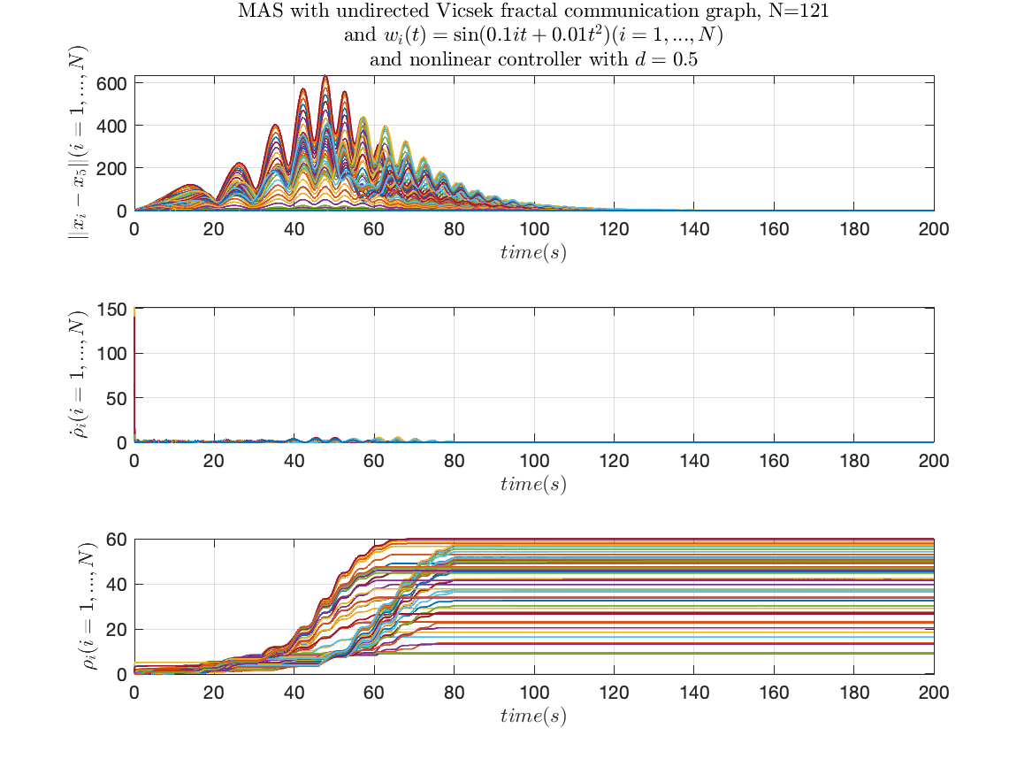
Figure 8: $\delta$-level coherent state synchronization of MAS with directed Vicsek fractal communication graphs and $N=121$ in the presence of disturbances via protocol (51) where $d=0.5$

IV-A2 Undirected graphs

Second, we consider undirected Vicsek fractal graphs. The algebraic connectivity of the undirected Vicsek fractal graphs is presented in Table I. It can be easily seen that the size of the graphs increase the algebraic connectivity of the associated Laplacian matrix decreases. The simulation results presented in Figure 6-8 show that the one-shot designed protocol (51), achieves $\delta-$level coherent state synchronization regardless of the number of agents and the algebraic connectivity of the associated Laplacian matrices of the graphs.

Table I: Algebraic connectivity of undirected Vicsek fractal graphs

$N$	g	$\operatorname{Re}\{\lambda_{2}\}$
5	1	1
25	2	0.0692
121	3	0.0053

IV-B Effectiveness with different types of communication graphs

In this example, we illustrate that the protocol that we designed for our MAS also achieves synchronization for different types of communication graphs. We considered MAS (50) with $N=121$ in the previous section where the agents are subject to noise (52). In this example, the agents are communicating through directed circulant graphs shown in Figure 2. Figure 9 shows the effectiveness of our designed protocol (51) for MAS with directed circulant communication graphs.

IV-C Robustness to different noise patterns

In this example, we analyze the robustness of our protocols to different noise patterns. As before, we consider MAS with $N=121$ in section IV-A communicating through directed Vicsek fractal graph. In this example, we assume that agents are subject to

$$w_{i}(t)=0.01it-round(0.01it),\quad i=1,\ldots,N.$$ (53)

Figure 10 shows that our designed protocol is robust even in the presence of noise with different pattern.

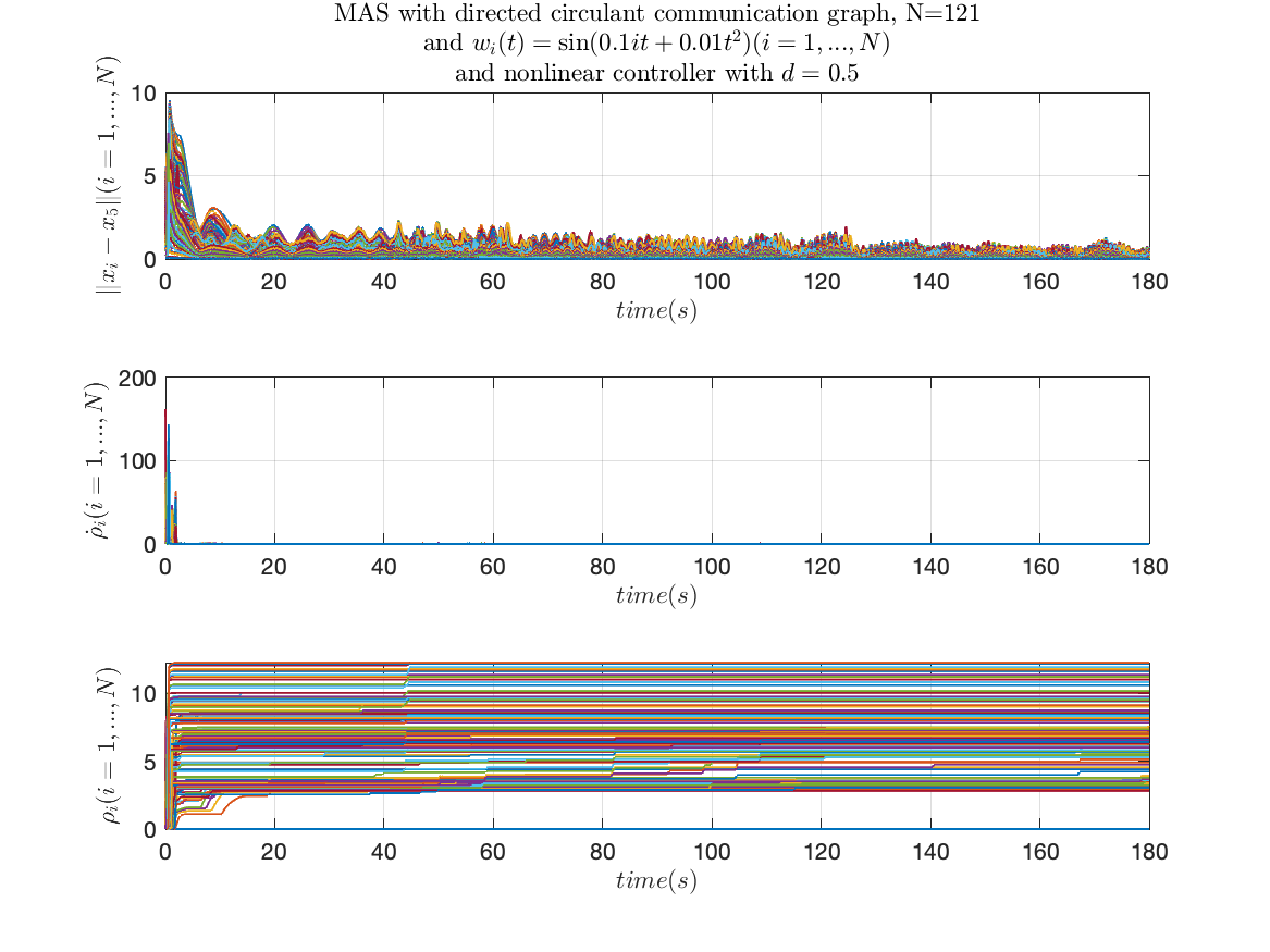
Figure 9: $\delta$-level coherent state synchronization of MAS with $N=121$ and directed circulant communication graphs in the presence of disturbances via nonlinear protocol with $d=0.5$

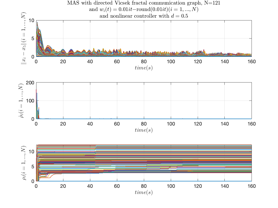
Figure 10: $\delta$-level coherent state synchronization of MAS with $N=121$ and directed Vicsek fractal communication graphs in the presence of disturbances $w_{i}=0.01it-round(0.01it)$ via nonlinear protocol with $d=0.5$

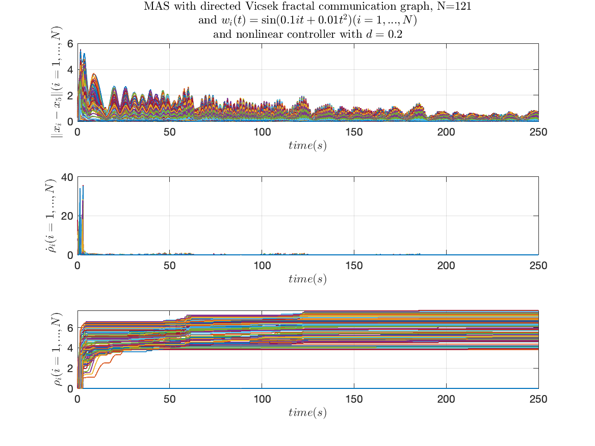
Figure 11: $\delta$-level coherent state synchronization of MAS with $N=121$ and directed Vicsek fractal communication graphs in the presence of disturbances via nonlinear protocol with $d=0.2$

IV-D Effectiveness for different d values

Finally, in this section, we show the effectiveness of the proposed protocol for different values of delta. Similar to the previous examples, we consider the MAS of section IV-A with $N=121$ communication through directed Vicsek fractal graphs where the agents are subject to noise (52). In this example, we choose $d=0.2$. The simulation results presented in Figure 11 show the effectiveness of our protocol independent of the value of $d$.

V Conclusion

This paper studied scalable $\delta-$level coherent state synchronization of MAS where agents were subject to bounded disturbances/noises. The results of this paper can be utilized in the string stability of vehicular platoon control and power systems. The directions for future research on scalable $\delta-$level coherent synchronization are: $1.$ Scalable $\delta-$level coherent synchronization of MAS with partial-state coupling; $2.$ Considering non input additive disturbance i.e., where $\operatorname{Im}E\not\subset\operatorname{Im}B$. The authors are conducting research in both directions.

References

• [1] H. Bai, M. Arcak, and J. Wen. Cooperative control design: a systematic, passivity-based approach. Communications and Control Engineering. Springer Verlag, 2011.
• [2] D. Chowdhury and H. K. Khalil. Synchronization in networks of identical linear systems with reduced information. In American Control Conference, pages 5706–5711, Milwaukee, WI, 2018.
• [3] C. Godsil and G. Royle. Algebraic graph theory, volume 207 of Graduate Texts in Mathematics. Springer-Verlag, New York, 2001.
• [4] H. Kim, H. Shim, J. Back, and J. Seo. Consensus of output-coupled linear multi-agent systems under fast switching network: averaging approach. Automatica, 49(1):267–272, 2013.
• [5] Z. Liu, D. Nojavanzadeh, D. Saberi, A. Saberi, and A. A. Stoorvogel. Regulated state synchronization for homogeneous networks of non-introspective agents in presence of input delays: a scale-free protocol design. In Chinese Control and Decision Conference, pages 856–861, Hefei, China, 2020.
• [6] Z. Liu, D. Nojavanzadeh, D. Saberi, A. Saberi, and A. A. Stoorvogel. Scale-free protocol design for regulated state synchronization of homogeneous multi-agent systems in presence of unknown and non-uniform input delays. Syst. & Contr. Letters, 152(104927), 2021.
• [7] Z. Liu, D. Nojavanzedah, and A. Saberi. Cooperative control of multi-agent systems: A scale-free protocol design. Springer, Cham, 2022.
• [8] Z. Liu, A. Saberi, A. A. Stoorvogel, and D. Nojavanzadeh. Global and semi-global regulated state synchronization for homogeneous networks of non-introspective agents in presence of input saturation. In Proc. 58th CDC, pages 7307–7312, Nice, France, 2019.
• [9] Z. Liu, A. Saberi, A.A. Stoorvogel, and D. Nojavanzadeh. $H_{\infty}$ almost state synchronization for homogeneous networks of non-introspective agents: a scale-free protocol design. Automatica, 122(109276):1–7, 2020.
• [10] Z. Liu, A. A. Stoorvogel, A. Saberi, and D. Nojavanzadeh. Squared-down passivity-based state synchronization of homogeneous continuous-time multiagent systems via static protocol in the presence of time-varying topology. Int. J. Robust & Nonlinear Control, 29(12):3821–3840, 2019.
• [11] Z. Liu, M. Zhang, A. Saberi, and A. A. Stoorvogel. State synchronization of multi-agent systems via static or adaptive nonlinear dynamic protocols. Automatica, 95:316–327, 2018.
• [12] M. Mesbahi and M. Egerstedt. Graph theoretic methods in multiagent networks. Princeton University Press, Princeton, 2010.
• [13] D. Nojavanzadeh, Z. Liu, A. Saberi, and A.A. Stoorvogel. Output and regulated output synchronization of heterogeneous multi-agent systems: A scale-free protocol design using no information about communication network and the number of agents. In American Control Conference, pages 865–870, Denver, CO, 2020.
• [14] R. Olfati-Saber and R.M. Murray. Consensus problems in networks of agents with switching topology and time-delays. IEEE Trans. Aut. Contr., 49(9):1520–1533, 2004.
• [15] E. Peymani, H.F. Grip, and A. Saberi. Homogeneous networks of non-introspective agents under external disturbances - $H_{\infty}$ almost synchronization. Automatica, 52:363–372, 2015.
• [16] E. Peymani, H.F. Grip, A. Saberi, X. Wang, and T.I. Fossen. $H_{\infty}$ almost ouput synchronization for heterogeneous networks of introspective agents under external disturbances. Automatica, 50(4):1026–1036, 2014.
• [17] Z. Qu. Cooperative control of dynamical systems: applications to autonomous vehicles. Spinger-Verlag, London, U.K., 2009.
• [18] W. Ren. On consensus algorithms for double-integrator dynamics. IEEE Trans. Aut. Contr., 53(6):1503–1509, 2008.
• [19] W. Ren and R.W. Beard. Consensus seeking in multiagent systems under dynamically changing interaction topologies. IEEE Trans. Aut. Contr., 50(5):655–661, 2005.
• [20] W. Ren and Y.C. Cao. Distributed coordination of multi-agent networks. Communications and Control Engineering. Springer-Verlag, London, 2011.
• [21] A. Saberi, A. A. Stoorvogel, M. Zhang, and P. Sannuti. Synchronization of multi-agent systems in the presence of disturbances and delays. Birkhäuser, New York, 2022.
• [22] L. Scardovi and R. Sepulchre. Synchronization in networks of identical linear systems. Automatica, 45(11):2557–2562, 2009.
• [23] J.H. Seo, J. Back, H. Kim, and H. Shim. Output feedback consensus for high-order linear systems having uniform ranks under switching topology. IET Control Theory and Applications, 6(8):1118–1124, 2012.
• [24] J.H. Seo, H. Shim, and J. Back. Consensus of high-order linear systems using dynamic output feedback compensator: low gain approach. Automatica, 45(11):2659–2664, 2009.
• [25] A. A. Stoorvogel, A. Saberi, Z. Liu, and D. Nojavanzadeh. ${H}_{2}$ and ${H}_{\infty}$ almost output synchronization of heterogeneous continuous-time multi-agent systems with passive agents and partial-state coupling via static protocol. Int. J. Robust & Nonlinear Control, 29(17):6244–6255, 2019.
• [26] A.A. Stoorvogel, A. Saberi, M. Zhang, and Z. Liu. Solvability conditions and design for $H_{\infty}$ and $H_{2}$ almost state synchronization of homogeneous multi-agent systems. European Journal of Control, 46:36–48, 2019.
• [27] Y. Su and J. Huang. Stability of a class of linear switching systems with applications to two consensus problem. IEEE Trans. Aut. Contr., 57(6):1420–1430, 2012.
• [28] S.E. Tuna. LQR-based coupling gain for synchronization of linear systems. Available: arXiv:0801.3390v1, 2008.
• [29] S.E. Tuna. Conditions for synchronizability in arrays of coupled linear systems. IEEE Trans. Aut. Contr., 55(10):2416–2420, 2009.
• [30] P. Wieland, J.S. Kim, and F. Allgöwer. On topology and dynamics of consensus among linear high-order agents. International Journal of Systems Science, 42(10):1831–1842, 2011.
• [31] C.W. Wu. Synchronization in complex networks of nonlinear dynamical systems. World Scientific Publishing Company, Singapore, 2007.
• [32] M. Zhang, A. Saberi, H. F. Grip, and A. A. Stoorvogel. $\mathcal{H}_{\infty}$ almost output synchronization for heterogeneous networks without exchange of controller states. IEEE Trans. Control of Network Systems, 2(4):348–357, 2015.
• [33] M. Zhang, A. Saberi, and A. A. Stoorvogel. Regulated output synchronization for heterogeneous time-varying networks with non-introspective agents in presence of disturbance and measurement noise with known frequencies. In American Control Conference, pages 2069–2074, Chicago, IL, 2015.
• [34] M. Zhang, A. Saberi, and A. A. Stoorvogel. Synchronization for heterogeneous time-varying networks with non-introspective, non-minimum-phase agents in the presence of external disturbances with known frequencies. In Proc. 55th CDC, pages 5201–5206, Las Vegas, NV, 2016.
• [35] M. Zhang, A. Saberi, A. A. Stoorvogel, and P. Sannuti. Almost regulated output synchronization for heterogeneous time-varying networks of non-introspective agents and without exchange of controller states. In American Control Conference, pages 2735–2740, Chicago, IL, 2015.
• [36] M. Zhang, A.A. Stoorvogel, and A. Saberi. Stochastic almost regulated output synchronization for time-varying networks of nonidentical and non-introspective agents under external stochastic disturbances and disturbances with known frequencies. In M.N. Belur, M.K. Camlibel, P. Rapisarda, and J.M.A. Scherpen, editors, Mathematical control theory II, volume 462 of Lecture Notes in Control and Information Sciences, pages 101–127. Springer Verlag, 2015.