Maintaining Plasticity in Continual Learning
via Regenerative Regularization

Abstract

In continual learning, plasticity refers to the ability of an agent to quickly adapt to new information. Neural networks are known to lose plasticity when processing non-stationary data streams. In this paper, we propose L$2$ Init, a simple approach for maintaining plasticity by incorporating in the loss function L2 regularization toward initial parameters. This is very similar to standard L$2$ regularization (L$2$), the only difference being that L$2$ regularizes toward the origin. L$2$ Init is simple to implement and requires selecting only a single hyper-parameter. The motivation for this method is the same as that of methods that reset neurons or parameter values. Intuitively, when recent losses are insensitive to particular parameters, these parameters should drift toward their initial values. This prepares parameters to adapt quickly to new tasks. On problems representative of different types of nonstationarity in continual supervised learning, we demonstrate that L$2$ Init most consistently mitigates plasticity loss compared to previously proposed approaches.

1 Introduction

In continual learning, an agent must continually adapt to an ever-changing data stream. Previous studies have shown that in non-stationary problems, neural networks tend to lose their ability to adapt over time (see e.g., Achille et al. [2017], Ash and Adams [2020], Dohare et al. [2021]). This is known as loss of plasticity. Methods proposed to mitigate this issue include those which continuously or periodically reset some subset of weights [Dohare et al., 2021, Sokar et al., 2023], add regularization to the training objective [Ash and Adams, 2020], or add architectural changes to the neural network [Ba et al., 2016, Lyle et al., 2023, Nikishin et al., 2023].

However, these approaches either fail on a broader set of problems or can be quite complicated to implement, with multiple moving parts or hyper-parameters to tune. In this paper, we draw inspiration from methods that effectively maintain plasticity in continual learning, such as Continual Backprop [Dohare et al., 2021], to propose a simpler regularization-based alternative. Our main contribution is a simple approach for maintaining plasticity that we call L$2$ Init. Our approach manifests as a simple modification to L2 regularization which is used throughout the deep learning literature. Rather than regularizing toward zero, L$2$ Init regularizes toward the initial parameter values. Specifically, our proposed regularization term is the squared L2 norm of the difference between the network’s current parameter values and the initial values. L$2$ Init is a simple method to implement that only requires one additional hyper-parameter.

The motivation for this approach is the same as that of methods that reset neurons or parameters, such as Continual Backprop. Intuitively, by ensuring that some parameter values are close to initialization, there are always parameters that can be recruited for rapid adaption to a new task. There are multiple reasons why having parameters close to initialization may increase plasticity, including maintaining smaller weight magnitudes, avoiding dead ReLU units, and preventing weight rank from collapsing.

To study L$2$ Init, we perform an empirical study on continual supervised learning problems, each exhibiting one of two types of non-stationarity: input distribution shift and target function (or concept) shift. We find that L$2$ Init most consistently retains high plasticity on both types of non-stationarity relative to other methods. To better understand the mechanism by which L$2$ Init maintains plasticity, we study how the average weight magnitude and feature rank evolve throughout training. While both L$2$ Init and standard L$2$ regularization reduce weight magnitude, L$2$ Init maintains high feature rank, a property that is sometimes correlated with retaining plasticity [Kumar et al., 2020]. Finally, in an ablation, we find that regularizing toward the fixed initial parameters rather than a random set of parameters is an important component of the method. Further, we find that using the L1 distance instead of L2 distance when regularizing towards initial parameters also significantly mitigates plasticity loss, but overall performance is slightly worse compared to L2 Init.

2 Related Work

Over the past decade, there has been emerging evidence that neural networks lose their capacity to learn over time when faced with nonstationary data streams [Ash and Adams, 2020, Dohare et al., 2021]. This phenomenon was first identified for deep learning in the context of pre-training [Achille et al., 2017, Zilly et al., 2020, Ash and Adams, 2020]. For instance, Achille et al. [2017] demonstrated that training a neural network on blurred CIFAR images significantly reduced its ability to subsequently learn on the original CIFAR images. Since then, the deterioration of neural networks’ learning capacity over time has been identified under various names, including the negative pre-training effect [Zilly et al., 2020], intransigence [Chaudhry et al., 2018], critical learning periods [Achille et al., 2017], the primacy bias [Nikishin et al., 2022], dormant neuron phenomenon [Sokar et al., 2023], implicit under-parameterization [Kumar et al., 2020], capacity loss [Lyle et al., 2022], and finally, the all-encompassing term, loss of plasticity (or plasticity loss) [Lyle et al., 2023]. In this section, we review problem settings in which plasticity loss has been studied, potential causes of plasticity loss, and methods previously proposed to mitigate this issue.

2.1 Problem Settings

We first review two problem settings in which plasticity loss has been studied: continual learning and reinforcement learning.

Continual Learning. In this paper, we aim to mitigate plasticity loss in the continual learning setting, and in particular, continual supervised learning. While the continual learning literature has primarily focused on reducing catastrophic forgetting [Goodfellow et al., 2013, Kirkpatrick et al., 2017], more recently, the issue of plasticity loss has gained significant attention [Dohare et al., 2021, 2023, Abbas et al., 2023]. Dohare et al. [2021] demonstrated that loss of plasticity sometimes becomes evident only after training for long sequences of tasks. Therefore, in continual learning, mitigating plasticity loss becomes especially important as agents encounter many tasks, or more generally a non-stationary data stream, over a long lifetime.

Reinforcement Learning. Plasticity loss has also gained significant attention in the deep reinforcement learning (RL) literature [Igl et al., 2020, Kumar et al., 2020, Nikishin et al., 2022, Lyle et al., 2022, Gulcehre et al., 2022, Sokar et al., 2023, Nikishin et al., 2023, Lyle et al., 2023]. In RL, the input data stream exhibits two sources of non-stationarity. First, observations are significantly correlated over time and are influenced by the agent’s policy which is continuously evolving. Second, common RL methods using temporal difference learning bootstrap off of the predictions of a periodically updating target network [Mnih et al., 2013]. The changing regression target introduces an additional source of non-stationarity.

2.2 Causes of plasticity loss

While there are several hypotheses for why neural networks lose plasticity, this issue remains poorly understood. Proposed causes include inactive ReLU units, feature or weight rank collapse, and divergence due to large weight magnitudes [Lyle et al., 2023, Sokar et al., 2023, Dohare et al., 2023, Kumar et al., 2020]. Dohare et al. [2021] suggest that using the Adam optimizer makes it difficult to update weights with large magnitude since updates are bounded by the step size. Zilly et al. [2021] propose that when both the incoming and outgoing weights of a neuron are close to zero, they are “mutually frozen” and will be very slow to update, which can result in reduced plasticity. However, both Lyle et al. [2023] and Gulcehre et al. [2022] show that many of the previously suggested mechanisms for loss of plasticity are insufficient to explain plasticity loss. While the causes of plasticity loss remain unclear, we believe it is possible to devise methods to mitigate the issue, drawing inspiration from the fact that initialized neural networks have high plasticity.

2.3 Mitigating plasticity loss

There have been about a dozen methods proposed for mitigating loss of plasticity. We categorize them into four main types: resetting, regularization, architectural, and optimizer solutions.

Resetting. This paper draws inspiration from resetting methods, which reinitialize subsets of neurons or parameters [Zilly et al., 2020, Dohare et al., 2021, Nikishin et al., 2022, 2023, Sokar et al., 2023, Dohare et al., 2023]. For instance, Continual Backprop [Dohare et al., 2021] tracks a utility measure for each neuron and resets neurons with utility below a certain threshold. This procedure involves multiple hyper-parameters, including the utility threshold, the maturity threshold, the replacement rate, and the utility decay rate. Sokar et al. [2023] propose a similar but simpler idea. Instead of tracking utilities for each neuron, they periodically compute the activations on a batch of data. A neuron is reset if it has small average activation relative to other neurons in the corresponding layer of the neural network. A related solution to resetting individual neurons is to keep a replay buffer and train a newly initialized neural network from scratch on data in the buffer [Igl et al., 2020], either using the original labels or using the current network’s outputs as targets. This is a conceptually simple but computationally very expensive method. Inspired by these approaches, the aim of this paper is to develop a simple regularization method that implicitly, and smoothly, resets weights with low utility.

Regularization. A number of methods have been proposed that regularize neural network parameters [Ash and Adams, 2020, Kumar et al., 2020, Lyle et al., 2022]. The most similar approach to our method is L2 regularization, which regularizes parameters towards zero. While L2 regularization reduces parameter magnitudes which helps mitigate plasiticy loss, regularizing toward the origin is likely to collapse the ranks of the weight matrices as well as lead to so-called mutually frozen weights [Zilly et al., 2021], both of which may have adverse effects on plasticity. In contrast, our regenerative regularization approach avoids these issues. Another method similar to ours is Shrink & Perturb [Ash and Adams, 2020] which is a two-step procedure applied at regular intervals. The weights are first shrunk by multiplying with a scalar and then perturbed by adding random noise. The shrinkage and noise scale factors are hyper-parameters. In Appendix A.3, we discuss the relationship between Shrink & Perturb and the regenerative regularization we propose. Additional regularization methods to mitigate plasticity loss include those proposed by Lyle et al. [2022], which regularizes a neural network’s output towards earlier predictions, and Kumar et al. [2020], which maximizes feature rank.

Lastly, we discuss Elastic Weight Consolidation (EWC) [Kirkpatrick et al., 2017] which was designed for mitigating catastrophic forgetting. EWC is similar our method, in that it regularizes towards previous parameters. An important difference, however, is that EWC does not regularize towards the initial parameters, but rather towards the parameters at the end of each previous task. Thus, while EWC is designed to remember information about previous tasks, our method is designed to maintain plasticity. Perhaps one can say that our method is designed to “remember how to learn.”

Architectural. Layer normalization [Ba et al., 2016], which is a common technique used throughout deep learning, has been shown to mitigate plasticity loss [Lyle et al., 2023]. A second solution aims to reduce the number of neural network features which consistently output zero by modifying the ReLU activation function [Shang et al., 2016, Abbas et al., 2023]. In particular, applying Concatenated ReLU ensures that each neuron is always activated and therefore has non-zero gradient. However, Concatenated ReLU comes at the cost of doubling the total number of parameters. In particular, each hidden layer output is concatenated with the negative of the output values before applying the ReLU activation, which doubles the number of inputs to the next layer. In our experiments in Section 5, we modify the neural network architecture of Concat ReLU such that it has the same parameter count as all other agents.

Optimizer. The Adam optimizer in its standard form is ill-suited for the continual learning setting. In particular, Adam tracks estimates of the first and second moments of the gradient, and these estimates can become inaccurate when the incoming data distribution changes rapidly. When training value-based RL agents, Lyle et al. [2023] evaluates the effects of resetting the optimizer state when the target network is updated. This alone did not mitigate plasticity loss. Another approach they evaluate is tuning Adam hyper-parameters such that second moment estimates are more rapidly updated and sensitivity to large gradients is reduced. While this significantly improved performance on toy RL problems, some plasticity loss remained. An important benefit of the method we propose is that it is designed to work with any neural network architecture and optimizer.

3 Regenerative Regularization

In this section, we propose a simple method for maintaining plasticity, which we call L$2$ Init. Our approach draws inspiration from prior works which demonstrate the benefits of selectively reinitializing parameters for retaining plasticity. The motivation for these approaches is that reinitialized parameters can be recruited for new tasks, and dormant or inactive neurons can regain their utility [Dohare et al., 2021, Nikishin et al., 2022, Sokar et al., 2023]. While these methods have enjoyed success across different problems, they often involve multiple additional components or hyper-parameters. In contrast, L$2$ Init is simple to implement and introduces a single hyper-parameter.

Given neural network parameters $\theta$, L$2$ Init augments a standard training loss function $\mathcal{L}_{\text{train}}(\theta)$ with a regularization term. Specifically, L$2$ Init performs L$2$ regularization toward initial parameter values $\theta_{0}$ at every time step for which a gradient update occurs. The augmented loss function is

$$\mathcal{L}_{\text{reg}}(\theta)=\mathcal{L}_{\text{train}}(\theta)+\lambda||\theta-\theta_{0}||_{2}^{2},$$

where $\lambda$ is the regularization strength and $\theta_{0}$ is the vector of parameter values at time step $0$.

Our regularization term is similar to standard L$2$ regularization, with the difference that L$2$ Init regularizes toward the initial parameter values instead of the origin. While this is a simple modification, we demonstrate in Section 5 that it significantly reduces plasticity loss relative to standard L$2$ regularization in continual learning settings.

L$2$ Init is similar in spirit to resetting methods such as Continual Backprop [Dohare et al., 2021], which explicitly computes a utility measure for each neuron and then resets neurons with low utility. Rather than resetting full neurons, L$2$ Init works on a per-weight basis, and encourages weights with low utility to reset. Intuitively, when the training loss $\mathcal{L}_{\text{train}}$ becomes insensitive to particular parameters, these parameters drift toward their initial values, preparing them to adapt quickly to future tasks. Thus, L$2$ Init can be thought of as implicitly and smoothly resetting low-utility weights. We use the term regenerative regularization to characterize regularization which rejuvenates parameters that are no longer useful.

4 Continual Supervised Learning

In this paper, we study plasticity loss in the continual supervised learning setting. In the continual supervised learning problems we consider, an agent is presented with a sequence $\{{\rm{T}}_{i}\}_{i=1}^{K}$ of $K$ tasks. Each task ${\rm{T}}_{i}$ corresponds to a unique dataset $\mathcal{D}_{{\rm{T}}_{i}}$ of (image, label) data pairs, and the agent receives a batch of samples from this dataset at each timestep, for a fixed duration of $M$ timesteps.

4.1 Evaluation Protocol

To measure both agents’ performance as well as their ability to retain plasticity, we measure the average online accuracy on each task. In particular, for each task ${\rm{T}}_{i}$, we compute

$$\text{Avg Online Task Accuracy}({\rm{T}}_{i})=\frac{1}{M}\sum_{j=t_{i}}^{t_{i}+M-1}a_{j}$$

where $t_{i}$ is the starting time step of task $T_{i}$ and $a_{j}$ is the average accuracy on the $j$th batch of samples. We refer to this metric as the average online task accuracy. This metric captures how quickly the agent is able to learn to do well on the task, which is a measure of its plasticity. If average online task accuracy goes down over time, we say that there is plasticity loss, assuming all tasks are of equal difficulty.

To perform model selection, we additionally compute each agent’s average online accuracy over all data seen in the agent’s lifetime. This is a common metric used in online continual learning [Cai et al., 2021, Ghunaim et al., 2023, Prabhu et al., 2023] and is computed as follows:

$$\text{Total Avg Online Accuracy}=\frac{1}{MK}\sum_{t=0}^{MK}a_{t}$$

To distinguish from average online task accuracy, we will refer to this metric as the total average online accuracy.

Plasticity loss encapsulates two related but distinct phenomena. First, it encompasses the reduction in a neural network’s capacity to fit incoming data. For instance, Lyle et al. [2023] show how a neural network trained using Adam optimizer significantly loses its ability to fit a dataset of MNIST images with randomly assigned labels. Second, plasticity loss also includes a reduction in a neural network’s capacity to generalize to new data [Igl et al., 2020, Liu et al., 2020]. The two metrics above will be sensitive to both of these phenomena.

4.2 Problems

In our experiments in Section 5, we evaluate methods on five continual image classification problems. Three of the problems, Permuted MNIST, 5+1 CIFAR, and Continual ImageNet exhibit input distribution shift, where different tasks have different inputs. The remaining problems, Random Label MNIST and Random Label CIFAR, exhibit concept shift, where different tasks have the exact same inputs but different labels assigned to each input. All continual image classification problems we consider consist of a sequence of supervised learning tasks. The agent is presented with batches of (image, label) data pairs from a task for a fixed number of timesteps, after which the next task arrives. The agent is trained incrementally to minimize cross-entropy loss on the batches it receives. While there are discrete task boundaries, the agent is not given any indication when a task switches.

Permuted MNIST. The first problem we consider is Permuted MNIST, a common benchmark from the continual learning literature [Goodfellow et al., 2013]. In our Permuted MNIST setup, we randomly sample 10,000 images from the MNIST training dataset. A Permuted MNIST task is characterized by applying a fixed randomly sampled permutation to the input pixels of all 10,000 images. The agent is presented with these 10,000 images in a sequence of batches, equivalent to training for $1$ epoch through the task’s dataset. After all samples have been seen once, the next task arrives, and the process repeats. In our Permuted MNIST experiments, we train agents for $500$ tasks.

Random Label MNIST. Our second problem is Random Label MNIST, a variation of the problem in Lyle et al. [2023]. We randomly sample $1200$ images from the MNIST dataset. A Random Label MNIST task is characterized by randomly assigning a label to each individual image in this subset. In contrast to Permuted MNIST, we train the agent for $400$ epochs such that the neural network learns to memorize the labels for the images. After $400$ epochs are complete, the next task arrives, and the process repeats. In our Random Label MNIST experiments, we train agents for $50$ tasks.

Random Label CIFAR. The third problem is Random Label CIFAR, which is equivalent to the setup of Random Label MNIST except that data is sampled from the CIFAR $10$ training dataset. For Permuted MNIST, Random Label MNIST, and Random Label CIFAR, data arrives in batches of size $16$.

5+1 CIFAR. In our fourth problem, 5+1 CIFAR, tasks have varying difficulty. Specifically, every even task is “hard” while every odd task is “easy.” Data is drawn from the CIFAR 100 dataset, and a hard task is characterized by seeing (image, label) data pairs of $5$ CIFAR 100 classes, whereas in an easy task, data from from only a single class arrives. Each hard task consists of $2500$ data pairs ($500$ from each class), while each easy tasks consists of $500$ data pairs from a single class. In particular, the tasks which have a single class are characterized as “easy” since all labels are the same. Each task has a duration of $780$ timesteps which corresponds to $10$ epochs through the hard task datasets when using a batch size of $32$. This problem is designed to reflect continual learning scenarios with varying input distributions, as agents receive data with varying levels of diversity at different times. In this problem, we measure agents’ performance specifically on the hard tasks since all agents do well on the easy tasks.

Continual ImageNet. The fifth problem is a variation of Continual ImageNet [Dohare et al., 2023], where each task is to distinguish between two ImageNet classes. Each task draws from a dataset of $1200$ images, $600$ from each of two classes. We train agents for $10$ epoch on each task using batch size $100$. In line with [Dohare et al., 2023], the images are downsized to 32 x 32 to save computation. In both 5+1 CIFAR and Continual ImageNet, each individual class does not occur in more than one task. Additional details of all problems are in Appendix A.1.1.

5 Experiments

The goal of our experiments is to determine whether L$2$ Init mitigates plasticity loss in continual supervised learning. To this end, we evaluate L$2$ Init and a selection of prior approaches on continual image classification problems introduced in Section 4.2, most of which have been previously used to study plasticity loss Dohare et al. [2021], Lyle et al. [2023]. We select methods which have shown good performance in previous work studying continual learning and which are representative of three different method types: resetting, regularization, and architectural solutions. These methods we consider are the following:

• Resetting: Continual Backprop [Dohare et al., 2021], ReDO [Sokar et al., 2023]

• Regularization: L$2$ Regularization (L$2$), Shrink & Perturb [Ash and Adams, 2020]

• Architectural: Concatenated ReLU (Concat ReLU) [Shang et al., 2016, Abbas et al., 2023], Layer Normalization (Layer Norm) [Ba et al., 2016]

Evaluation. On all problems, we perform a hyper-parameter sweep for each method and average results over $3$ seeds. For each method, we select the configuration that resulted in the largest total average online accuracy. We then run the best configuration for each method on $10$ additional seeds, which produces the results in Figures 1-5. In addition to determinining the initialization of the neural network, each seed also determines the problem parameters, such as the data comprising each task, and the sequence of sampled (data, label) from each task’s dataset. For instance, on Permuted MNIST, the seed determines a unique sequence of permutations applied to the images resulting in a unique task sequence, as well as how the task data is shuffled. As another example, on Continual ImageNet, it determines the pairs of classes that comprise each task, the sequence of tasks, and the sequence of batches in each task. For all problems, the seed determines a unique set of tasks and sequence of those tasks.

Hyper-parameters. To evaluate robustness to the choice of optimizer, we train all agents with both Adam and Stochastic Gradient Descent with fixed step size (Vanilla SGD). We choose Adam because it is one of the most common optimizers in deep learning, and we choose Vanilla SGD because recent work has argued against the use of Adam in continual learning [Ashley et al., 2021]. For all agents, we sweep over stepsizes $\alpha\in\{1\mathrm{e}{-2},1\mathrm{e}{-3}\}$ when using Vanilla SGD and $\alpha\in\{1\mathrm{e}{-3},1\mathrm{e}{-4}\}$ when using Adam. We additionally sweep over $\alpha=0.1$ when using Vanilla SGD on 5+1 CIFAR and Continual ImageNet. For L$2$ and L$2$ Init, we sweep over regularization strength $\lambda\in\{1\mathrm{e}{-2},1\mathrm{e}{-3},1\mathrm{e}{-4},1\mathrm{e}{-5}\}$. For Shrink & Perturb, we perform a grid search over shrinkage parameter $p\in\{1\mathrm{e}{-2},1\mathrm{e}{-3},1\mathrm{e}{-4},1\mathrm{e}{-5}\}$ and noise scale $\sigma\in\{1\mathrm{e}{-2},1\mathrm{e}{-3},1\mathrm{e}{-4},1\mathrm{e}{-5}\}$. For Continual Backprop, we sweep over the replacement rate $r\in\{1\mathrm{e}{-4},1\mathrm{e}{-5},1\mathrm{e}{-6}\}$. For all other Continual Backprop hyper-parameters, we use the values reported in Dohare et al. [2023]. For ReDO, we sweep over the recycle period by recycling neurons either every $1$, $2$, or $5$ tasks, and we sweep over the recycle threshold in the set $\{0,0.01,0.1\}$. Finally, as baseline methods, we run vanilla incremental SGD with constant stepsize and Adam. Other than the stepsize, we use the PyTorch default hyperparameters for both optimizers. Additional training details, including neural network architectures and hyper-parameter settings, are in Appendix A.1.2.

5.1 Comparative Evaluation

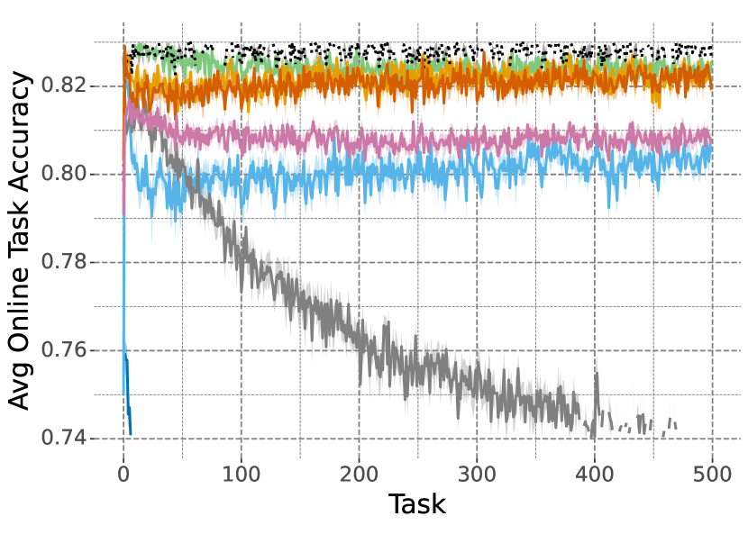
Permuted MNIST

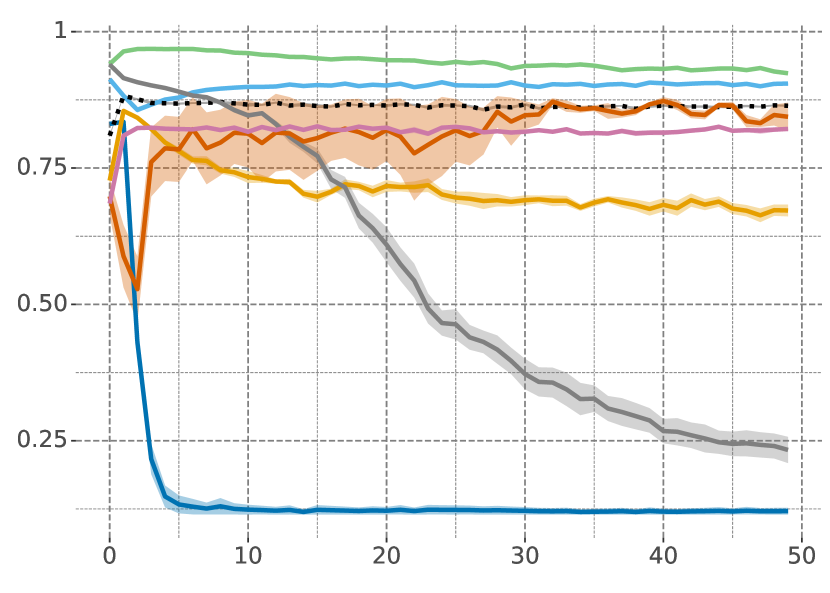
Random Label MNIST

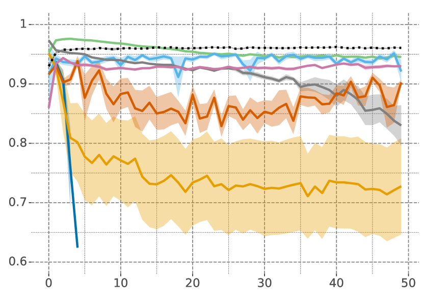
Random Label CIFAR

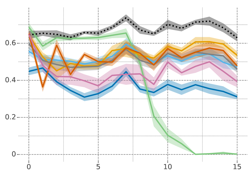
5+1 CIFAR

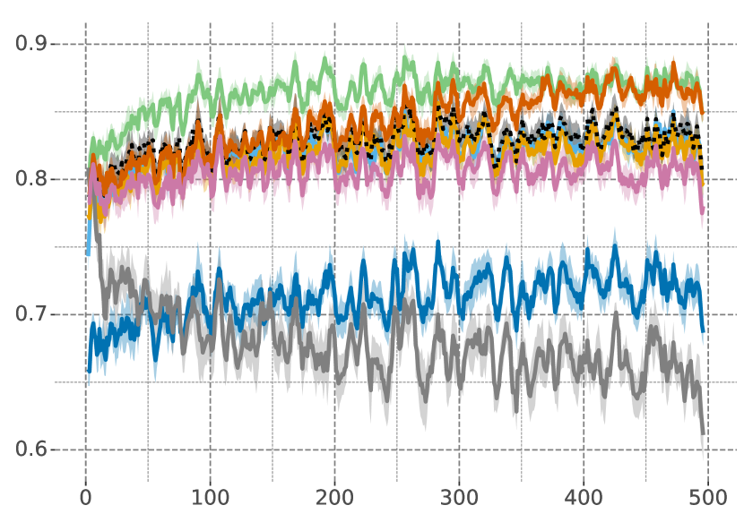
Continual ImageNet

Figure 1: Comparison of average online task accuracy across all five problems when using the Adam optimizer. L$2$ Init consistently maintains plasticity. While L$2$ mitigates plasticity loss completely on Permuted MNIST and Continual ImageNet, this method performs poorly on Random Label MNIST, Random Label CIFAR, and 5+1 CIFAR. Concat ReLU generally performs very well, except on 5+1 CIFAR where it suffers a sharp drop in performance.

L2 Init

Concat ReLU

Continual Backprop

ReDO

L2

Shrink and Perturb

Layer Norm

Baseline

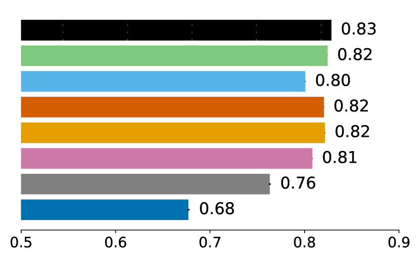
Permuted MNIST

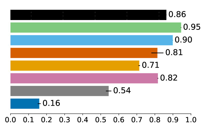
Random Label MNIST

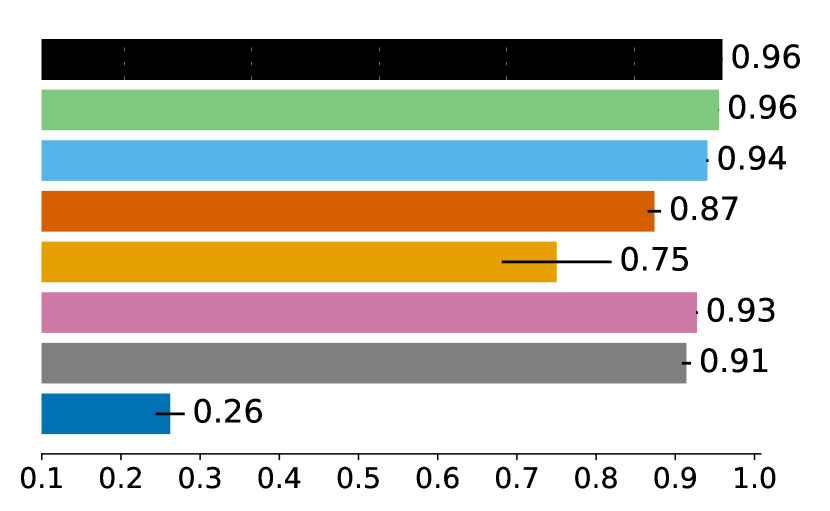
Random Label CIFAR

L2 Init

Concat ReLU

Continual Backprop

ReDO

L2

Shrink and Perturb

Layer Norm

Baseline

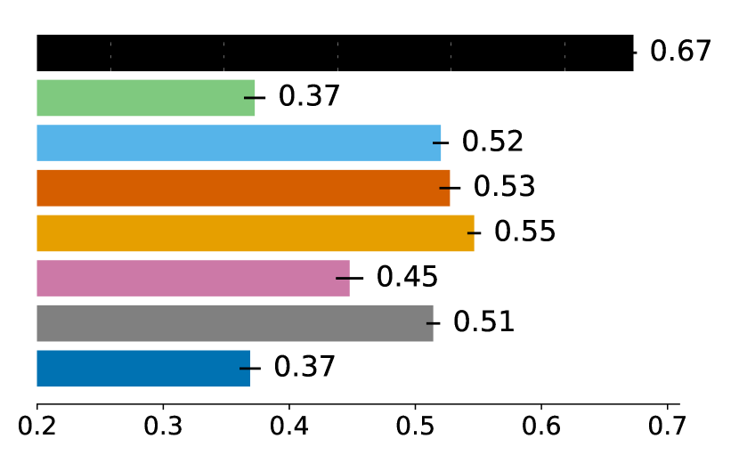
5+1 CIFAR

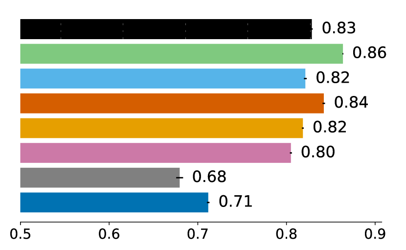
Continual ImageNet

Figure 2: Comparison of total average online accuracy across all five problems when using the Adam optimizer. L$2$ Init performs in the top 3 in each of the five environments. On 5+1 CIFAR, it significantly outperforms all other methods. Concat ReLU does well on all problems except for 5+1 CIFAR.

Results with Adam. We plot the average online task accuracy and the total average online task accuracy for all methods when using Adam in Figures 1 and 2. On all five problems, the Baseline method either significantly loses plasticity over time or performs poorly overall. Because we select hyperparameters based on total average online accuracy, the baseline method is sometimes be run with a smaller learning rate which results in low plasticity loss but still relatively poor performance. Importantly, L$2$ Init consistently retains high plasticity across problems and maintains high average online task accuracy throughout training. L$2$ Init has comparable performance to the two resetting methods Continual Backprop and ReDO. Specifically, it performs as well as or better than Continual Backprop on four out of the five problems. The same roughly holds true when comparing to the performance of ReDO.

Concat ReLU performs well on all problems except 5+1 CIFAR on which it loses plasticity completely. Concat ReLU loses some plasticity on Random Label MNIST and Random Label CIFAR, but the overall performance is still quite high. While L2 significantly mitigates plasticity loss on Permuted MNIST, there is still large plasticity loss on Random Label MNIST, Random Label CIFAR, and 5+1 CIFAR as compared to L$2$ Init. Shrink & Perturb does mitigate plasticity loss on all problems, but overall performance is consistently lower than that of L$2$ Init. Finally, Layer Norm mitigates only some plasticity loss.

Permuted MNIST

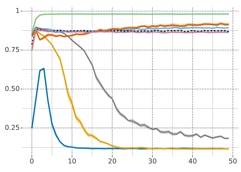
Random Label MNIST

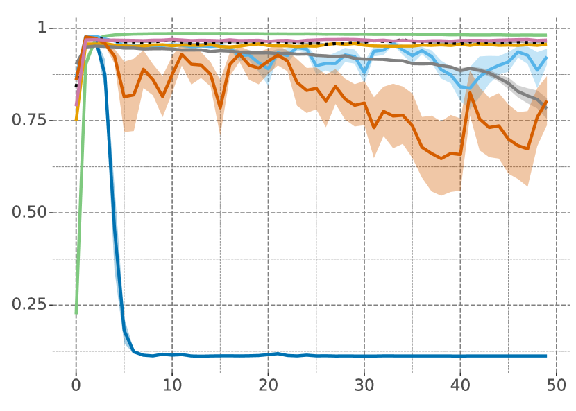
Random Label CIFAR

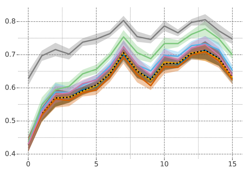
5+1 CIFAR

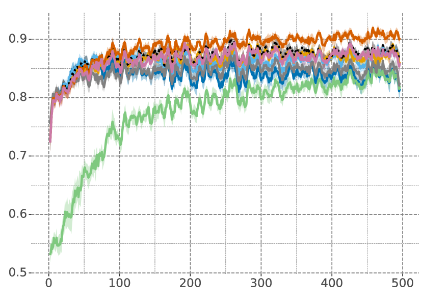
Continual ImageNet

Figure 3: Comparison of average online task accuracy across all five problems when using Vanilla SGD. L$2$ Init consistently maintains plasticity, whereas L2 does not on Permuted MNIST and Random Label MNIST.

Results with Vanilla SGD. Compared to when using Adam, there is less plasticity loss when using Vanilla SGD, as shown in Figure 3. L$2$ Init performs similarly to Continual Backprop and consistently mitigates plasticity on problems on which it occurs. In contrast, L2 does not on Permuted MNIST and Random Label MNIST. L$2$ Init also performs similarly to ReDO, although ReDO’s performance has larger variation between seeds. Concat ReLU performs well across problems but loses plasticity on Permuted MNIST and has lower performance on Continual ImageNet. Unlike when using Adam, L2 Init does not outperform all methods on 5+1 CIFAR. Instead, Layer Norm performs the best on this problem.

5.2 Looking inside the network

Permuted MNIST		Random Label MNIST
Weight Magnitude	Feature SRank	Weight Magnitude	Feature SRank
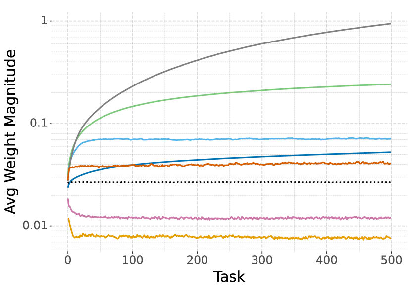
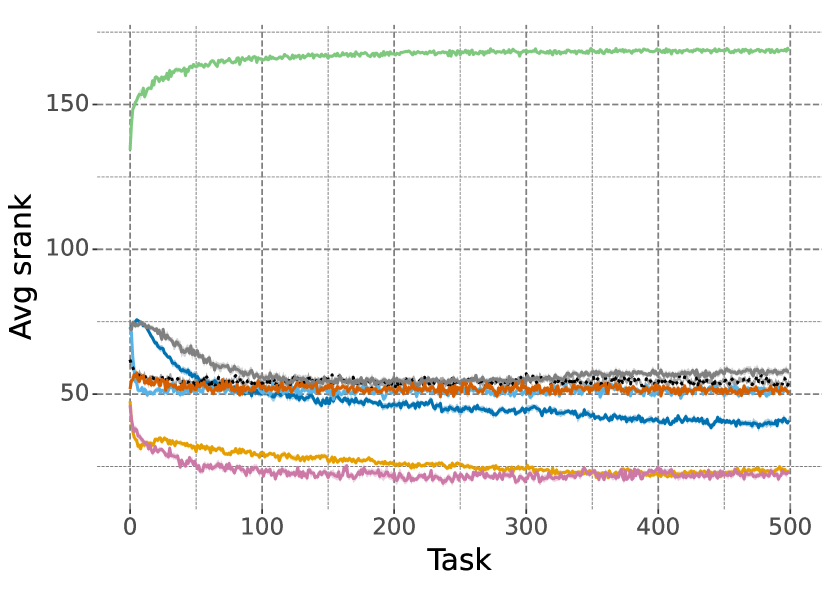
5+1 CIFAR		Continual ImageNet
Weight Magnitude	Feature SRank	Weight Magnitude	Feature SRank

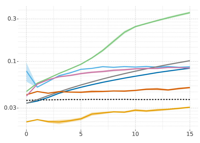
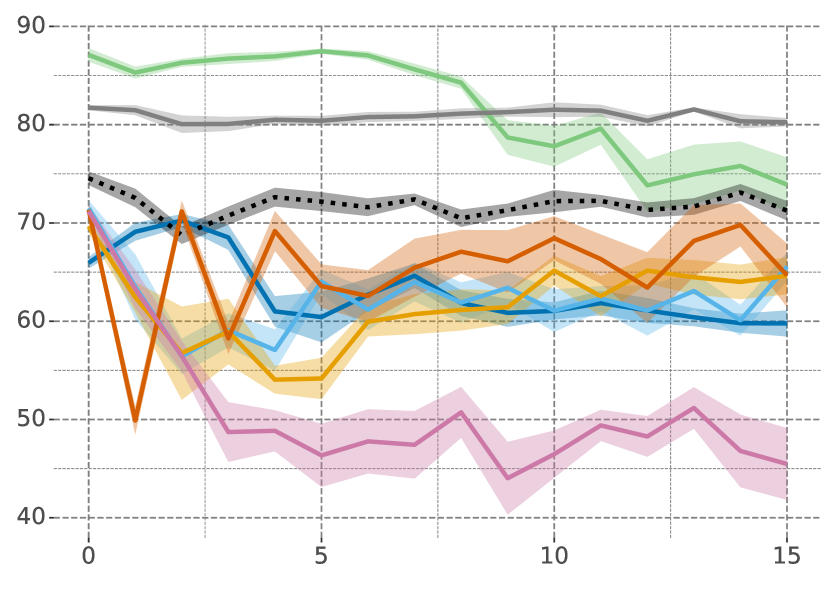
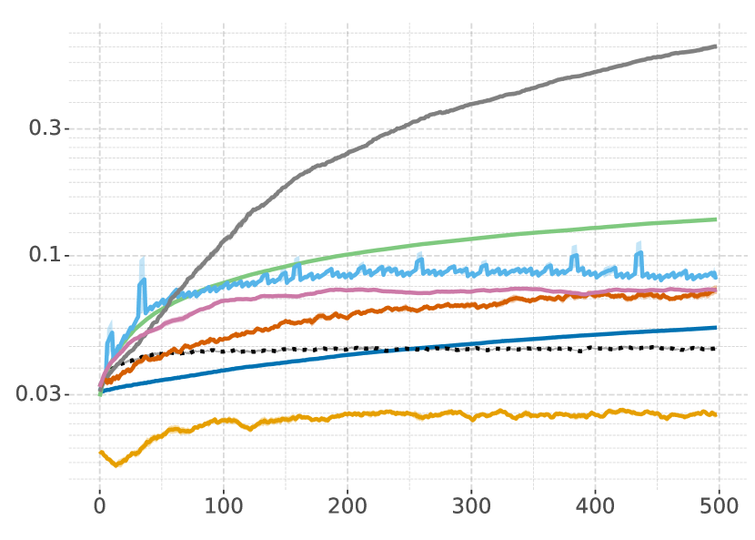
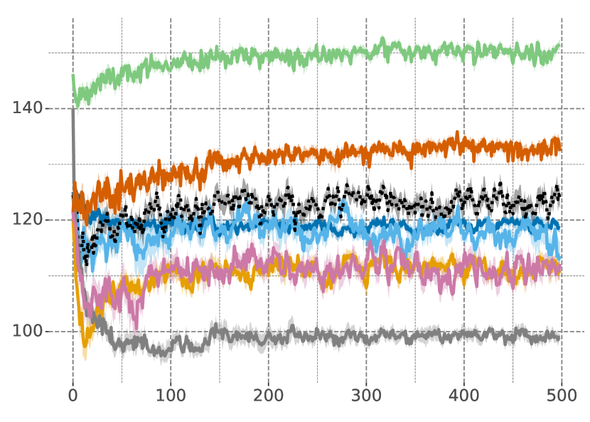
Figure 4: Average weight magnitude and feature rank over time when training all agents using Adam. L$2$ Init retains a relatively small average weight magnitude and high feature rank.

While the causes of plasticity loss remain unclear, it is likely that large parameter magnitudes as well as a reduction in feature rank can play a role. For instance, ReLU units that stop activating regardless of input will have zero gradients and will not be updated, therefore potentially not adapting to future tasks. To understand how L$2$ Init affects neural network dynamics, we plot the average weight magnitude (L1 norm) as well as the average feature rank computed at the end of each task on four problems when training using the Adam optimizer (Figure 4).

A measure of the effective rank of a matrix, that Kumar et al. [2020] call srank, is computed from the singular values of the matrix. Specifically, using the ordered set of singular values $\sigma_{1}>\sigma_{2},...\sigma_{n}$, we compute the srank as

$$\text{srank}=\min_{k}\frac{\sum_{i=1}^{k}\sigma_{i}}{\sum_{j=1}^{n}\sigma_{j}}\geq 1-\delta$$

using the threshold $\delta=0.01$ following Kumar et al. [2020]. Thus, in this case, the srank is how many singular values you need to sum up to make up $99\%$ of the total sum of singular values.

In Figure 4, we see that both L$2$ Init and L2 reduce the average weight magnitude relative to the Baseline. As pointed out by Dohare et al. [2021], this is potentially important when using the Adam optimizer. Since the updates with Adam are bounded by the global stepsize or a small multiple of the global stepsize, when switching to a new task, the relative change in these weights may be small. However, agents which perform quite well such Continual Backprop and Concat ReLU result in surprisingly large average weight magnitude, making any clear takeaway lacking. However, on 5+1 CIFAR the weight magnitude of Concat ReLU is very large relative to other methods, potentially explaining its sharp drop in performance in Figure 1.

When using L$2$, the effective feature rank is smaller than it is when applying L$2$ Init. This is to be expected since L$2$ Init is regularizing towards a set of full-rank matrices, and could potentially contribute to the increased plasticity we see with L$2$ Init. Notably, Concat ReLU enjoys high feature rank across problems (with the exception of 5+1 CIFAR) which is potentially contributing to its high performance.

5.3 Ablation Study of Regenerative Regularization

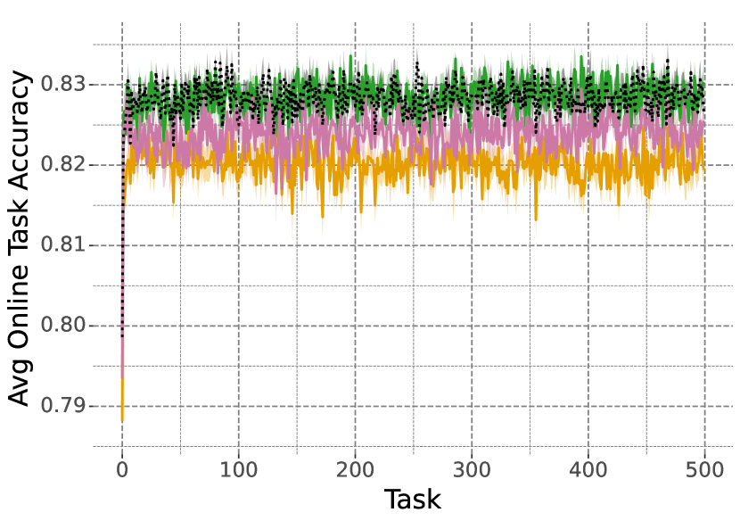
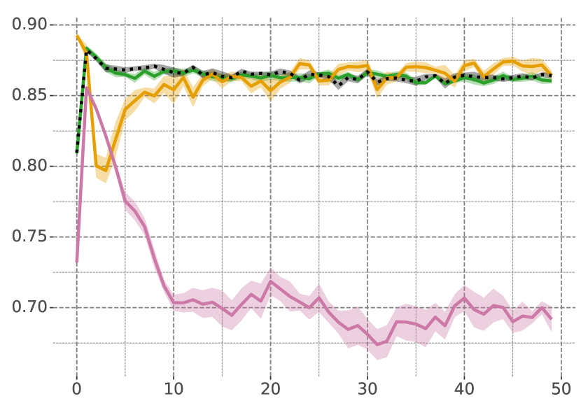
	Permuted MNIST	Random Label MNIST	5+1 CIFAR

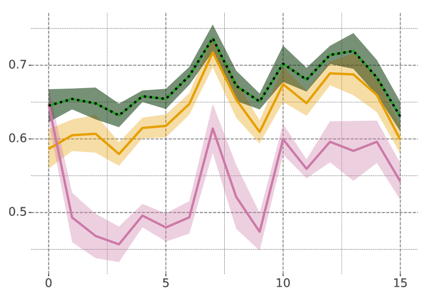
Figure 5: Comparison of L2 Init, L2 Init + Resample, L1 Init, and Huber Init on three problems when using Adam. L2 Init + Resample performs poorly on all environments, especially on Random Label MNIST and 5+1 CIFAR where it loses plasticity. L1 Init matches the performance of L2 Init on Random Label MNIST and performs slightly worse on Permuted MNIST and 5+1 CIFAR. Huber Init matches the performance of L2 Init on all three problems.

Regularizing toward random parameters

With L$2$ Init, we regularize toward the specific fixed parameters $\theta_{0}$ sampled at initialization. Following a procedure more similar to Shrink & Perturb, we could alternatively sample a new set of parameters at each time step. That is, we could sample $\phi_{t}$ from the same distribution that $\theta_{0}$ was sampled from and let the regularization term be $||\theta_{t}-\phi_{t}||_{2}^{2}$ instead. In Figure 5, we compare the performance between L$2$ Init and this variant (L$2$ Init + Resample) on Permuted MNIST, Random Label MNIST, and 5+1 CIFAR when using the Adam optimizer. We select the best regularization strength for each method using the same hyper-parameter sweep used for L$2$ Init. We find that regularizing towards the initial parameters rather than sampling a new set of parameters at each time step performs much better.

Choice of norm

While L$2$ Init uses the L2 norm, we could alternatively use the L1 norm of the difference between the parameters and their initial values. We call this approach L1 Init, which uses the following loss function:

$$\mathcal{L}_{\text{reg}}(\theta)=\mathcal{L}_{\text{train}}(\theta)+\lambda||\theta-\theta_{0}||_{1}$$

As another alternative, we could apply the Huber loss to balance between L1 Init and L2 Init. We call this approach Huber Init, which uses the following loss function:

$$\mathcal{L}_{\text{reg}}(\theta)=\mathcal{L}_{\text{train}}(\theta)+\lambda\text{Huber}(\theta,\theta_{0})$$

We compare the performance of L$2$ Init, L1 Init, and Huber Init on Permuted MNIST, Random Label MNIST, 5+1 CIFAR, and Continual ImageNet when using the Adam optimizer (see Figure 4). We find that while L1 Init mitigates plasticity loss, the performance is worse on Permuted MNIST and 5+1 CIFAR. The performance of Huber Init matches that of L2 Init.

6 Conclusion

Recently, multiple methods have been proposed for mitigating plasticity loss in continual learning. One common and quite successful category of methods is characterized by periodically re-initializing subsets of weights. However, resetting methods bring additional decisions to be made by the algorithm designer, such as which parameters to reinitialize and how often. In this paper, we propose a very simple alternative that we call L$2$ Init. Concretely, we add a loss term that regularizes the parameters toward the initial parameters. This encourages parameters that have little influence on recent losses to drift toward initialization and therefore allows them to be recruited for future adaptation. This approach is similar to standard L2 regularization, but rather than regularizing toward the origin, we regularize toward the initial parameters, which ensures that the weight rank does not collapse. To evaluate L$2$ Init, we perform an empirical study on three simple continual learning problems. We compare L$2$ Init with a set of previously proposed methods. L$2$ Init consistently maintains plasticity and almost matches the performance of Continual Backprop. Aside from Continual Backprop, the other methods we compare with all lose plasticity on at least one of the problems or perform substantially worse overall.

We hope our method opens up avenues for future work on mitigating plasticity loss. In future work, it would be useful to evaluate L$2$ Init on a broader set of problems, including regression and RL settings. It is possible that our method may need to be adjusted, for instance by using L1 instead of L2 regularization. Finally, this study has focused exclusively on maintaining plasticity, leaving aside the issue of forgetting. In practical applications, mitigating forgetting and maintaining plasticity are both crucial. Therefore, in future work, it is important to study plasticity and forgetting in tandem. This can be accomplished perhaps by considering problems in which there is significant forward transfer, that is in which information learned on earlier tasks is helpful for future tasks. In such problems, it is likely that techniques for increasing plasticity come at the cost of increased forgetting. Designing methods that effectively balance the trade-off between maintaining plasticity and avoiding forgetting is an exciting avenue for future work.

Appendix A Appendix

A.1 Experiment Details

A.1.1 Problems

Parameters for each of the five problems we consider are listed in Table 1.

Permuted MNIST
Parameter	Value
dataset size per task	10,000 samples
batch size	$16$
task duration	$625$ timesteps ($1$ epoch)
number of tasks	$500$

Random Label MNIST & Random Label CIFAR
Parameter	Value
dataset size per task	$1200$ samples
batch size	$16$
task duration	30,000 timesteps ($400$ epochs)
number of tasks	$50$

5+1 CIFAR
Parameter	Value
dataset size per hard task	$2500$ samples
dataset size per easy task	$500$ samples
batch size	$32$
task duration	780 timesteps
number of tasks	$30$ ($15$ hard, $15$ easy)

Continual ImageNet
Parameter	Value
dataset size per task	$1200$ samples
batch size	$100$
task duration	120 timesteps ($10$ epochs)
number of tasks	$500$

Table 1: Problem parameters.

A.1.2 Agents

Neural network architectures. For all agents, we used an MLP on Permuted MNIST and Random Label MNIST and a CNN on Random Label CIFAR, 5+1 CIFAR, and Continual ImageNet. We chose networks with small hidden layer width to study the setting in which plasticity loss is exacerbated due to capacity constraints. In particular, the neural network can achieve high average online task accuracy on a single task, or even a sequence of tasks, but when faced with a long sequence, plasticity loss occurs. The MLP and CNN architectures we use are as follows:

• MLP: We use two hidden layers of width $100$ and ReLU activations.

• CNN: We use two convolutional layers followed by two fully-connected layers. The first convolutional layer uses kernel size $5\times 5$ with $16$ output channels. This layer is followed by a max pool. The second also uses kernel size $5\times 5$ with $16$ output channels and is also followed by a max pool. The fully-connected layers have widths $100$.

• All networks have a fully connected output layer at the end with $10$ outputs for Permuted MNIST, Random Label MNIST, and Random Label CIFAR, $100$ outputs for 5+1 CIFAR, and $2$ outputs for Continual ImageNet.

The exception to the above is Concat ReLU, for which we use a slightly smaller hidden size since otherwise Concat ReLU would have twice the number of parameters as all other agents. Specifically, we compute the smallest fraction of neurons to remove from each hidden layer such that the total number of parameters in the network is as least as large as the ones in the above architectures. These fractions are $0.09$ on Permuted MNIST and Random Label MNIST, $0.27$ on Random Label CIFAR and Continual ImageNet, and $0.31$ on 5+1 CIFAR.

Hyper-parameters As described in Section 5, for all agents on all problems, we performed a hyper-parameter sweep over $3$ seeds for each problem and optimizer combination. The optimal hyper-parameter configurations based on the total average online accuracy metric are listed in Tables 2 and 3. We used these hyper-parameters with $10$ additional seeds to obtain all results.

Continual Backprop. For Continual Backprop, we use the implementation in the public GitHub repository. We try two different methods for computing utility. The first one, called “contribution,” uses the inverse of the average weight magnitude as a measure of utility. The second one, “adaptive-contribution,” is the one proposed in Dohare et al. [2021] that also utilizes the activation magnitude multiplied by the outgoing weights. See  Dohare et al. [2021, 2023] (and the associated GitHub repository) for additional details. There was barely any difference in performance between the two utility types, so we present the results for the type presented in their paper. The other Continual Backprop hyper-parameter settings we use are those reported in Dohare et al. [2023]. In particular, we set the maturity threshold to be $100$ and the utility decay rate to be $0.99$.

A.2 Additional Results

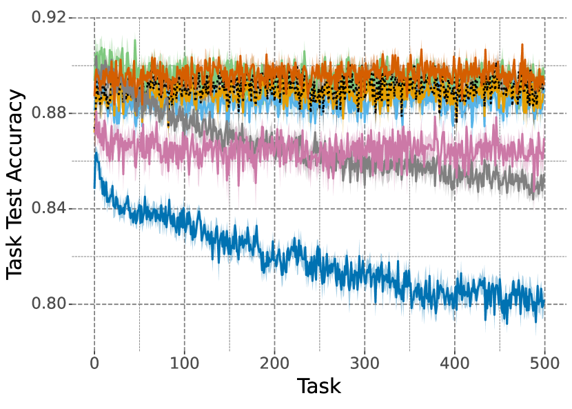
Permuted MNIST

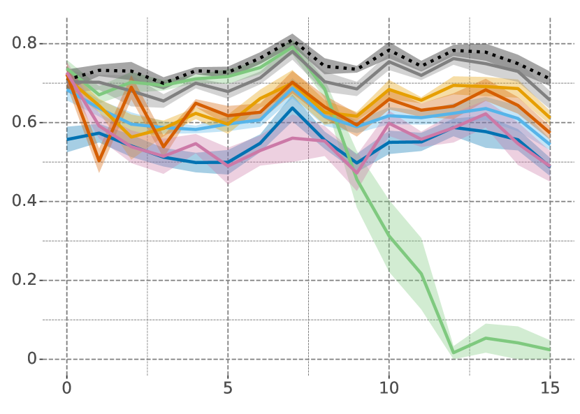
5+1 CIFAR

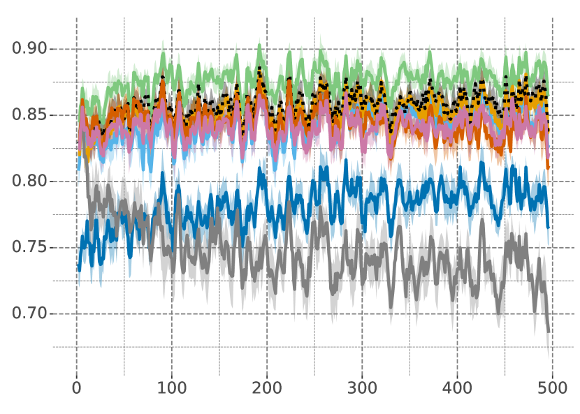
Continual ImageNet

Figure 6: Accuracy computed on held out task test data at the end of each task when training all agents with Adam. L$2$ Init consistently maintains plasticity and performs similarly to the other resetting methods Continual Backprop and ReDO. Concat ReLU performs well on Continual ImageNet but poorly on 5+1 CIFAR.

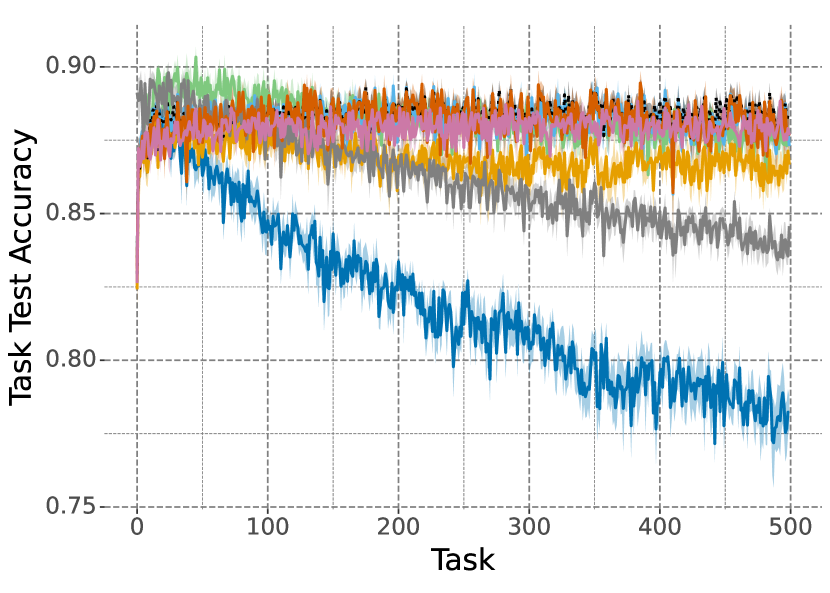
Permuted MNIST

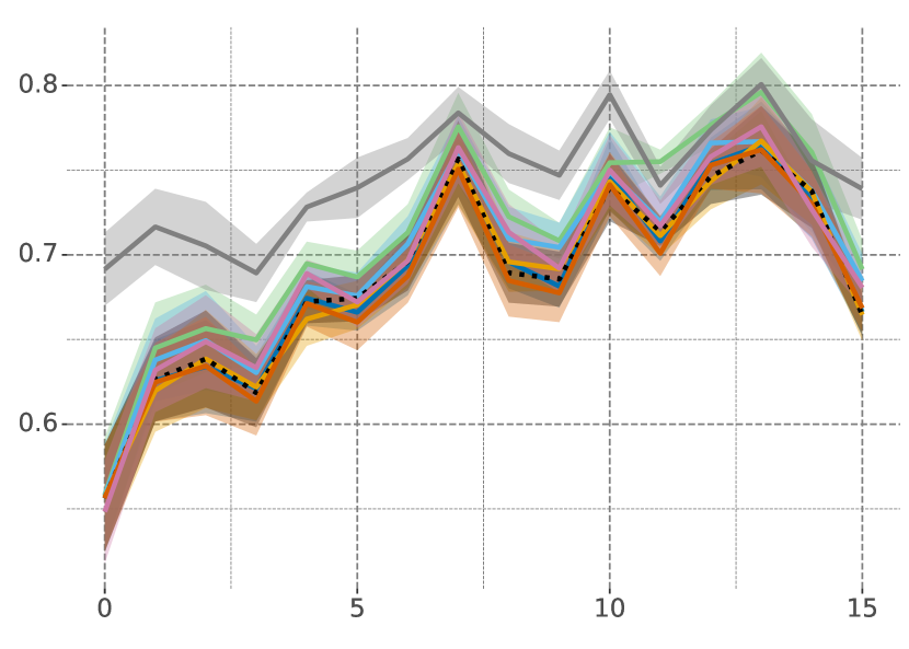
5+1 CIFAR

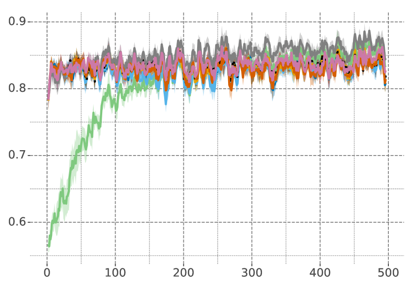
Continual ImageNet

Figure 7: Accuracy computed on held out task test data at the end of each task when training all agents with Vanilla SGD. While the results are mixed, L2 Init maintains good performance whereas L2 performs poorly on Permuted MNIST.

On problems which have test datasets (Permuted MNIST, 5+1 CIFAR, and Continual ImageNet), we additionally plot the test accuracy on each task in Figures 6 and 7. Specifically, at the end of each task, we compute the accuracy on the test data for that task. The generalization performance of L2 Init is consistently similar to that of the other resetting methods Continual Backprop and ReDO.

A.3 Connection to Shrink and Perturb

In Ash and Adams [2020], the Shrink and Perturb method was proposed to mitigate loss of plasticity. Every time a task switches, Shrink and Perturb multiplies neural network parameters by a shrinkage factor $p<1$ and then perturbs them by a small noise vector $\epsilon$. The Shrink and Perturb procedure is applied to the neural network when a task switches but can in principle be applied after every gradient step with a larger value of $p$. The update applied to the parameters $\theta_{t}$ at timestep $t$ is

$$\theta_{t+1}=\underbrace{p}_{\text{Shrink}}(\underbrace{\theta_{t}-\alpha\nabla\mathcal{L}_{\text{train}}(\theta_{t})}_{\text{SGD update}})+\underbrace{\sigma\epsilon}_{\text{Perturb}}$$

where $\epsilon$ is a noise vector and $\sigma$ is a scaling factor of the noise.

Ash and Adams [2020] suggest sampling $\epsilon$ from the same distribution that the neural network parameters were sampled from at initialization and then scaling with $\sigma$ which is a hyperparameter. This is to ensure that the noise magnitude scales appropriately with the width and type of the neural network layer corresponding to each individual parameter.

Before making the connection to our method, we will rewrite the Shrink and Perturb update rule further:

$$\theta_{t+1}=\underbrace{p\theta_{t}}_{\text{Shrink}}+\underbrace{\sigma\epsilon}_{\text{Perturb}}-\alpha\underbrace{p}_{\text{Shrink}}\nabla\mathcal{L}_{\text{train}}(\theta_{t})$$

where we instead shrink both $\theta_{t}$ and shrink the gradient.

When using SGD with a constant stepsize $\alpha$, our method can be written on a form that is quite similar to this. Specifically, when applying L$2$ Init, we can write the update to the parameters $\theta_{t}$ at timestep $t$ as

$$\theta_{t+1}=\underbrace{(1-\alpha\lambda)\theta_{t}}_{\text{Shrink}}+\underbrace{\alpha\lambda\theta_{0}}_{\text{Perturb}}-\alpha\nabla\mathcal{L}_{\text{train}}(\theta_{t})$$

where $\theta_{0}$ are the initial parameters at time step $0$, rather than random noise, and where the gradient is not shrunk. This form can be derived by taking the gradient of the L$2$ Init augmented loss function, plugging it into the SGD update rule, and factoring out $\theta_{t}$.

There are four seemingly small, but important, differences between L$2$ Init and Shrink and Perturb. First, our method has only one hyperparameter $\lambda$ rather than two. That is because the shrinkage and noise scaling factors are tied to $\lambda$: $p=(1-\alpha\lambda)$ and $\sigma=\alpha\lambda$. Further, both the shrinkage and noise scale parameters are tied to the step size. Second, our method regularizes toward the initial parameters, rather than toward a random sample from the initial distribution. Third, the gradient is not shrunk. Finally, when using Adam, the above connection between the two methods no longer holds for the same reason that L$2$ regularization and weight decay are not equivalent when using Adam.

Optimal Hyper-parameters on Permuted MNIST
Agent	Optimizer	Optimal Hyper-parameters
Baseline	SGD	$\alpha=1\mathrm{e}{-2}$
Layer Norm	SGD	$\alpha=1\mathrm{e}{-2}$
L$2$ Init	SGD	$\alpha=1\mathrm{e}{-2}$, $\lambda=1\mathrm{e}{-2}$
L2	SGD	$\alpha=1\mathrm{e}{-2}$, $\lambda=1\mathrm{e}{-2}$
Shrink & Perturb	SGD	$\alpha=1\mathrm{e}{-2}$, $p=1-1\mathrm{e}{-4}$, $\sigma=1\mathrm{e}{-2}$
Continual Backprop	SGD	$\alpha=1\mathrm{e}{-2}$, $r=1\mathrm{e}{-4}$
Concat ReLU	SGD	$\alpha=1\mathrm{e}{-2}$
ReDO	SGD	$\alpha=1\mathrm{e}{-2}$, recycle period = 625, recycle threshold = 0
Baseline	Adam	$\alpha=1\mathrm{e}{-4}$
Layer Norm	Adam	$\alpha=1\mathrm{e}{-3}$
L$2$ Init	Adam	$\alpha=1\mathrm{e}{-3}$, $\lambda=1\mathrm{e}{-2}$
L2 Origin	Adam	$\alpha=1\mathrm{e}{-3}$, $\lambda=1\mathrm{e}{-2}$
Shrink & Perturb	Adam	$\alpha=1\mathrm{e}{-3}$, $p=1-1\mathrm{e}{-3}$, $\sigma=1\mathrm{e}{-2}$
Continual Backprop	Adam	$\alpha=1\mathrm{e}{-3}$, $r=1\mathrm{e}{-4}$
Concat ReLU	Adam	$\alpha=1\mathrm{e}{-3}$
ReDO	Adam	$\alpha=1\mathrm{e}{-3}$, recycle period = 625, recycle threshold = 0

Optimal Hyper-parameters on Random Label MNIST
Agent	Optimizer	Optimal Hyper-parameters
Baseline	SGD	$\alpha=1\mathrm{e}{-3}$
Layer Norm	SGD	$\alpha=1\mathrm{e}{-3}$
L$2$ Init	SGD	$\alpha=1\mathrm{e}{-2}$, $\lambda=1\mathrm{e}{-2}$
L2	SGD	$\alpha=1\mathrm{e}{-2}$, $\lambda=1\mathrm{e}{-2}$
Shrink and Perturb	SGD	$\alpha=1\mathrm{e}{-2}$, $p=1-1\mathrm{e}-4$, $\sigma=1\mathrm{e}{-2}$
Continual Backprop	SGD	$\alpha=1\mathrm{e}{-2}$, $r=1\mathrm{e}{-4}$
Concat ReLU	SGD	$\alpha=1\mathrm{e}{-2}$
ReDO	SGD	$\alpha=1\mathrm{e}{-2}$, recycle period = 30000, recycle threshold = 0.1
Baseline	Adam	$\alpha=1\mathrm{e}{-4}$
Layer Norm	Adam	$\alpha=1\mathrm{e}{-4}$
L$2$ Init	Adam	$\alpha=1\mathrm{e}{-4}$, $\lambda=1\mathrm{e}{-2}$
L2	Adam	$\alpha=1\mathrm{e}{-4}$, $\lambda=1\mathrm{e}{-2}$
Shrink and Perturb	Adam	$\alpha=1\mathrm{e}{-4}$, $p=1-1\mathrm{e}{-4}$, $\sigma=1\mathrm{e}{-2}$
Continual Backprop	Adam	$\alpha=1\mathrm{e}{-3},r=1\mathrm{e}{-4}$
Concat ReLU	Adam	$\alpha=1\mathrm{e}{-3}$
ReDO	Adam	$\alpha=1\mathrm{e}{-3}$, recycle period = 30000, recycle threshold = 0.1

Optimal Hyper-parameters on Random Label CIFAR
Agent	Optimizer	Optimal Hyper-parameters
Baseline	SGD	$\alpha=1\mathrm{e}{-2}$
Layer Norm	SGD	$\alpha=1\mathrm{e}{-2}$
L$2$ Init	SGD	$\alpha=1\mathrm{e}{-2}$, $\lambda=1\mathrm{e}{-2}$
L2	SGD	$\alpha=1\mathrm{e}{-2}$, $\lambda=1\mathrm{e}{-2}$
Shrink & Perturb	SGD	$\alpha=1\mathrm{e}{-2}$, $p=1-1\mathrm{e}{-4}$, $\sigma=1\mathrm{e}{-2}$
Continual Backprop	SGD	$\alpha=1\mathrm{e}{-2},r=1\mathrm{e}{-4}$
Concat ReLU	SGD	$\alpha=1\mathrm{e}{-3}$
ReDO	SGD	$\alpha=1\mathrm{e}{-2}$, recycle period = 30000, recycle threshold = 0.1
Baseline	Adam	$\alpha=1\mathrm{e}{-3}$
Layer Norm	Adam	$\alpha=1\mathrm{e}{-3}$
L$2$ Init	Adam	$\alpha=1\mathrm{e}{-3}$, $\lambda=1\mathrm{e}{-2}$
L2	Adam	$\alpha=1\mathrm{e}{-4}$, $\lambda=1\mathrm{e}{-2}$
Shrink & Perturb	Adam	$\alpha=1\mathrm{e}{-3}$, $p=1-1\mathrm{e}{-4}$, $\sigma=1\mathrm{e}{-2}$
Continual Backprop	Adam	$\alpha=1\mathrm{e}{-3},r=1\mathrm{e}{-4}$
Concat ReLU	Adam	$\alpha=1\mathrm{e}{-3}$
ReDO	Adam	$\alpha=1\mathrm{e}{-4}$, recycle period = 30000, recycle threshold = 0.1

Table 2: Agent optimal hyper-parameters on Permuted MNIST, Random Label MNIST, and Random Label CIFAR. For each agent, we a hyper-parameter sweep over $3$ seeds and selected the hyper-parameters which corresponded to maximum total average online accuracy, averaged across the $3$ seeds.

Optimal Hyper-parameters on 5+1 CIFAR
Agent	Optimizer	Optimal Hyper-parameters
Baseline	SGD	$\alpha=1\mathrm{e}{-2}$
Layer Norm	SGD	$\alpha=0.1$
L$2$ Init	SGD	$\alpha=1\mathrm{e}{-2}$, $\lambda=1\mathrm{e}{-5}$
L2	SGD	$\alpha=1\mathrm{e}{-2}$, $\lambda=1\mathrm{e}{-4}$
Shrink & Perturb	SGD	$\alpha=1\mathrm{e}{-2}$, $p=1-1\mathrm{e}{-5}$, $\sigma=1\mathrm{e}{-2}$
Continual Backprop	SGD	$\alpha=1\mathrm{e}{-2}$, $r=1\mathrm{e}{-4}$
Concat ReLU	SGD	$\alpha=1\mathrm{e}{-2}$
ReDO	SGD	$\alpha=1\mathrm{e}{-2}$, recycle period = 1560, recycle threshold = 0
Baseline	Adam	$\alpha=1\mathrm{e}{-4}$
Layer Norm	Adam	$\alpha=1\mathrm{e}{-4}$
L$2$ Init	Adam	$\alpha=1\mathrm{e}{-3}$, $\lambda=1\mathrm{e}{-2}$
L2 Origin	Adam	$\alpha=1\mathrm{e}{-3}$, $\lambda=1\mathrm{e}{-3}$
Shrink & Perturb	Adam	$\alpha=1\mathrm{e}{-3}$, $p=1-1\mathrm{e}{-4}$, $\sigma=1\mathrm{e}{-2}$
Continual Backprop	Adam	$\alpha=1\mathrm{e}{-3}$, $r=1\mathrm{e}{-4}$
Concat ReLU	Adam	$\alpha=1\mathrm{e}{-3}$
ReDO	Adam	$\alpha=1\mathrm{e}{-3}$, recycle period = 1560, recycle threshold = 0

Optimal Hyper-parameters on Continual ImageNet
Agent	Optimizer	Optimal Hyper-parameters
Baseline	SGD	$\alpha=0.1$
Layer Norm	SGD	$\alpha=0.1$
L$2$ Init	SGD	$0.1$, $\lambda=1\mathrm{e}{-3}$
L2	SGD	$0.1$, $\lambda=1\mathrm{e}{-3}$
Shrink and Perturb	SGD	$\alpha=0.1$, $p=1-1\mathrm{e}{-4}$, $\sigma=1\mathrm{e}{-4}$
Continual Backprop	SGD	$\alpha=0.1$, $r=1\mathrm{e}{-4}$
Concat ReLU	SGD	$\alpha=1\mathrm{e}{-2}$
ReDO	SGD	$\alpha=0.1$, recycle period = 600, recycle threshold = 0.1
Baseline	Adam	$\alpha=1\mathrm{e}{-4}$
Layer Norm	Adam	$\alpha=1\mathrm{e}{-3}$
L$2$ Init	Adam	$\alpha=1\mathrm{e}{-3}$, $\lambda=1\mathrm{e}{-3}$
L2	Adam	$\alpha=1\mathrm{e}{-3}$, $\lambda=1\mathrm{e}{-3}$
Shrink and Perturb	Adam	$\alpha=1\mathrm{e}{-3}$, $p=1-1\mathrm{e}{-4}$, $\sigma=1\mathrm{e}{-2}$
Continual Backprop	Adam	$\alpha=1\mathrm{e}{-3},r=1\mathrm{e}{-4}$
Concat ReLU	Adam	$\alpha=1\mathrm{e}{-3}$
ReDO	Adam	$\alpha=1\mathrm{e}{-3}$, recycle period = 120, recycle threshold = 0

Table 3: Agent optimal hyper-parameters on 5+1 CIFAR and Continual ImageNet. For each agent, we a hyper-parameter sweep over $3$ seeds and selected the hyper-parameters which corresponded to maximum total average online accuracy, averaged across the $3$ seeds.

References

- Abbas et al. [2023] Zaheer Abbas, Rosie Zhao, Joseph Modayil, Adam White, and Marlos C Machado. Loss of plasticity in continual deep reinforcement learning. arXiv preprint arXiv:2303.07507, 2023.
- Achille et al. [2017] Alessandro Achille, Matteo Rovere, and Stefano Soatto. Critical learning periods in deep neural networks. arXiv preprint arXiv:1711.08856, 2017.
- Ash and Adams [2020] Jordan Ash and Ryan P Adams. On warm-starting neural network training. Advances in neural information processing systems, 33:3884–3894, 2020.
- Ashley et al. [2021] Dylan R Ashley, Sina Ghiassian, and Richard S Sutton. Does the Adam optimizer exacerbate catastrophic forgetting? arXiv preprint arXiv:2102.07686, 2021.
- Ba et al. [2016] Jimmy Lei Ba, Jamie Ryan Kiros, and Geoffrey E Hinton. Layer normalization. arXiv preprint arXiv:1607.06450, 2016.
- Cai et al. [2021] Zhipeng Cai, Ozan Sener, and Vladlen Koltun. Online continual learning with natural distribution shifts: An empirical study with visual data. In Proceedings of the IEEE/CVF international conference on computer vision, pages 8281–8290, 2021.
- Chaudhry et al. [2018] Arslan Chaudhry, Puneet K Dokania, Thalaiyasingam Ajanthan, and Philip HS Torr. Riemannian walk for incremental learning: Understanding forgetting and intransigence. In Proceedings of the European conference on computer vision (ECCV), pages 532–547, 2018.
- Dohare et al. [2021] Shibhansh Dohare, Richard S Sutton, and A Rupam Mahmood. Continual backprop: Stochastic gradient descent with persistent randomness. arXiv preprint arXiv:2108.06325, 2021.
- Dohare et al. [2023] Shibhansh Dohare, J Fernando Hernandez-Garcia, Parash Rahman, Richard S Sutton, and A Rupam Mahmood. Maintaining plasticity in deep continual learning. arXiv preprint arXiv:2306.13812, 2023.
- Ghunaim et al. [2023] Yasir Ghunaim, Adel Bibi, Kumail Alhamoud, Motasem Alfarra, Hasan Abed Al Kader Hammoud, Ameya Prabhu, Philip HS Torr, and Bernard Ghanem. Real-time evaluation in online continual learning: A new paradigm. arXiv preprint arXiv:2302.01047, 2023.
- Goodfellow et al. [2013] Ian J Goodfellow, Mehdi Mirza, Da Xiao, Aaron Courville, and Yoshua Bengio. An empirical investigation of catastrophic forgetting in gradient-based neural networks. arXiv preprint arXiv:1312.6211, 2013.
- Gulcehre et al. [2022] Caglar Gulcehre, Srivatsan Srinivasan, Jakub Sygnowski, Georg Ostrovski, Mehrdad Farajtabar, Matt Hoffman, Razvan Pascanu, and Arnaud Doucet. An empirical study of implicit regularization in deep offline RL. arXiv preprint arXiv:2207.02099, 2022.
- Igl et al. [2020] Maximilian Igl, Gregory Farquhar, Jelena Luketina, Wendelin Boehmer, and Shimon Whiteson. Transient non-stationarity and generalisation in deep reinforcement learning. arXiv preprint arXiv:2006.05826, 2020.
- Kirkpatrick et al. [2017] James Kirkpatrick, Razvan Pascanu, Neil Rabinowitz, Joel Veness, Guillaume Desjardins, Andrei A Rusu, Kieran Milan, John Quan, Tiago Ramalho, Agnieszka Grabska-Barwinska, et al. Overcoming catastrophic forgetting in neural networks. Proceedings of the national academy of sciences, 114(13):3521–3526, 2017.
- Kumar et al. [2020] Aviral Kumar, Rishabh Agarwal, Dibya Ghosh, and Sergey Levine. Implicit under-parameterization inhibits data-efficient deep reinforcement learning. arXiv preprint arXiv:2010.14498, 2020.
- Liu et al. [2020] Shengchao Liu, Dimitris Papailiopoulos, and Dimitris Achlioptas. Bad global minima exist and SGD can reach them. Advances in Neural Information Processing Systems, 33:8543–8552, 2020.
- Lyle et al. [2022] Clare Lyle, Mark Rowland, and Will Dabney. Understanding and preventing capacity loss in reinforcement learning. arXiv preprint arXiv:2204.09560, 2022.
- Lyle et al. [2023] Clare Lyle, Zeyu Zheng, Evgenii Nikishin, Bernardo Avila Pires, Razvan Pascanu, and Will Dabney. Understanding plasticity in neural networks. arXiv preprint arXiv:2303.01486, 2023.
- Mnih et al. [2013] Volodymyr Mnih, Koray Kavukcuoglu, David Silver, Alex Graves, Ioannis Antonoglou, Daan Wierstra, and Martin Riedmiller. Playing Atari with deep reinforcement learning. arXiv preprint arXiv:1312.5602, 2013.
- Nikishin et al. [2022] Evgenii Nikishin, Max Schwarzer, Pierluca D’Oro, Pierre-Luc Bacon, and Aaron Courville. The primacy bias in deep reinforcement learning. In International conference on machine learning, pages 16828–16847. PMLR, 2022.
- Nikishin et al. [2023] Evgenii Nikishin, Junhyuk Oh, Georg Ostrovski, Clare Lyle, Razvan Pascanu, Will Dabney, and André Barreto. Deep reinforcement learning with plasticity injection. arXiv preprint arXiv:2305.15555, 2023.
- Prabhu et al. [2023] Ameya Prabhu, Zhipeng Cai, Puneet Dokania, Philip Torr, Vladlen Koltun, and Ozan Sener. Online continual learning without the storage constraint. arXiv preprint arXiv:2305.09253, 2023.
- Shang et al. [2016] Wenling Shang, Kihyuk Sohn, Diogo Almeida, and Honglak Lee. Understanding and improving convolutional neural networks via concatenated rectified linear units. In international conference on machine learning, pages 2217–2225. PMLR, 2016.
- Sokar et al. [2023] Ghada Sokar, Rishabh Agarwal, Pablo Samuel Castro, and Utku Evci. The dormant neuron phenomenon in deep reinforcement learning. arXiv preprint arXiv:2302.12902, 2023.
- Zilly et al. [2021] Julian Zilly, Alessandro Achille, Andrea Censi, and Emilio Frazzoli. On plasticity, invariance, and mutually frozen weights in sequential task learning. Advances in Neural Information Processing Systems, 34:12386–12399, 2021.
- Zilly et al. [2020] Julian G Zilly, Franziska Eckert, Bhairav Mehta, Andrea Censi, and Emilio Frazzoli. The negative pretraining effect in sequential deep learning and three ways to fix it. 2020.