Abstract

It is known that global climate models (GCMs) have substantial biases in the surface freshwater flux which forces the ocean component of these models. Using numerical bifurcation analyses on a global ocean model, we study here the effect of a specific freshwater flux bias on the multiple equilibrium regime of the Atlantic Meridional Overturning Circulation (AMOC). We find that a (positive) freshwater flux bias over the Indian Ocean shifts the multiple equilibrium regime to larger values of North Atlantic freshwater input but hardly affects the associated hysteresis width. The magnitude of this shift depends on the way the anomalous North Atlantic freshwater flux is compensated. We explain the changes in bifurcation diagrams using the freshwater balance over the Atlantic basin. The results suggest that state-of-the-art GCMs may have an AMOC multiple equilibrium regime, but that it is located in a parameter regime that is considered unrealistic and hence is not explored.

1 Introduction

The AMOC has been proposed as one of the tipping elements in the climate system Lenton et al. (2008); Armstrong McKay et al. (2022), indicating that it may undergo a relatively rapid change under a slowly developing forcing. The AMOC is thought to be particularly sensitive to its freshwater forcing, either through the surface freshwater flux, through input of freshwater due to ice melt (e.g. from the Greenland Ice Sheet) or through river runoff Rahmstorf et al. (2005). These freshwater fluxes affect the ocean density differences which control the AMOC strength and change the heat and salt transport carried by AMOC Marotzke (2000).

From conceptual models, the tipping behaviour is clearly related to the multi-stability properties of the AMOC. For example, in the Stommel two-box model Stommel (1961), there is an interval of surface freshwater forcing where two stable steady AMOC states exist and tipping occurs due to transitions between these states. The central feedback responsible for the tipping behaviour is the salt-advection feedback, where a freshwater perturbation in the North Atlantic causes a weakening of the AMOC which leads to less northward salt transport and hence amplification of the perturbation Marotzke (2000).

Precise boundaries of the multiple-equilibrium regime of the AMOC have been obtained using conceptual models Cessi (1994); Cimatoribus et al. (2012) and fully-implicit ocean-climate models De Niet et al. (2007); Toom et al. (2012); Mulder et al. (2021). One of the important results of these studies is that the existence of the multiple-equilibrium regime can be related (in these models) to an observable quantity Rahmstorf (1996), now often called the AMOC stability (or regime) indicator. This indicator has many different notations in the literature, e.g. $M_{ov}$ De Vries and Weber (2005) or $F_{ov}$ Hawkins et al. (2011). Here, we will follow Weijer et al. (2019) and use $F_{ovS}$ ($F_{ovN}$) as the freshwater transport carried by the AMOC over the southern (northern) boundary at 35^∘S (60^∘N) of the Atlantic basin Dijkstra (2007); Huisman et al. (2010); Liu et al. (2017). Available observations Bryden et al. (2011) show that the present-day AMOC is exporting freshwater out of the Atlantic ($F_{ovS}<0$). It is known that $F_{ovS}$ ignores some relevant processes Gent (2018), but if one accepts that $F_{ovS}$ is a proper indicator, the AMOC is in a multiple-equilibrium regime based its observed values Weijer et al. (2019).

Less precise estimates of the multiple-equilibrium regime boundaries can be obtained from global climate models. In so-called quasi-equilibrium experiments, the freshwater forcing is changed very slowly such that the model state stays close to the (slowly changing) equilibrium. When the freshwater forcing is varied in both directions and covers the multiple-equilibrium regime, regime boundaries can be inferred from the so-called hysteresis width, i.e. the freshwater forcing values where the AMOC collapses and recovers. The rate of forcing is important here and if this is much faster than the equilibration time scale of the steady state, the approximations of the regime boundaries become worse and also rate-induced tipping may occur Lohmann et al. (2021). Such quasi-equilibrium experiments have been performed with many Earth System Models of Intermediate Complexity (EMICs) Rahmstorf et al. (2005) and the FAMOUS model, the latter being a GCM with a relatively coarse horizontal resolution of $2.5^{\circ}\times 3.75^{\circ}$ Hawkins et al. (2011). The Community Climate System Model (CCSM3) is probably the most detailed model in which AMOC hysteresis behavior has been investigated Hu et al. (2012).

Mostly due to computational constraints, often only the AMOC response to particular freshwater forcing perturbations is considered in state-of-the-art GCMs. In these so-called ‘hosing experiments’ Stouffer et al. (2006), quite a diversity of model behavior is found. It is not known whether a multiple-equilibrium AMOC regime exists in such models and only sporadic indications of such a regime have been found Mecking et al. (2016); Jackson and Wood (2018a, b). The problem is that it is difficult to assess whether the weak AMOC states computed are equilibrium solutions of the models. What these model studies certainly have shown is that an AMOC weakening would have severe impacts on the climate system, affecting sea level and regional temperatures in many areas around the world Vellinga et al. (2002); Jackson et al. (2015); Liu et al. (2020); Orihuela-Pinto et al. (2022).

Of course, the real present-day AMOC may not have a multiple equilibrium regime and GCMs may model that correctly. On the other hand, the real AMOC may be in such a regime, and the GCMs may not capture it. In that case, the GCMs misrepresent (or miss) crucial processes, such that they do not display tipping behaviour. A prominent example is the incorrect representation of ocean eddy transport processes in GCMs, which may prevent the existence of a multi-stable AMOC regime. Another possibility is that GCMs capture the relevant processes but the parameters in the models are not correct, such that a multi-stable regime does not occur due to model biases. An example of this is that many GCMs are considered to have a too stable AMOC due to biases in the freshwater transport in the Atlantic Ocean Drijfhout et al. (2013); Mecking et al. (2016).

In van Westen and Dijkstra (2023), it was shown that several persistent biases in state-of-the art climate models, of the Coupled Model Intercomparison Projects (CMIP) version 6, lead to an AMOC with an Atlantic freshwater transport that is in disagreement with observations (i.e., many models have $F_{ovS}>0$). The most important model bias is the surface freshwater flux over the Indian Ocean, which affects the freshwater transport at 34^∘S in the Atlantic through Agulhas Leakage. Motivated by these results, we revisit the bifurcation analysis on the global ocean-climate model Dijkstra (2007) and determine the effects of Indian Ocean surface freshwater flux biases on the multi-stable regime of the AMOC. In section 2, the fully-implicit model used is shortly summarised and the continuation methodology to compute bifurcation diagrams is described. Then in section 3, we focus on the effect of freshwater biases on the bifurcation diagrams. Mechanisms of the shift in the multi-stable regimes are analysed using the freshwater balance over the Atlantic. A summary and discussion follows in section 4.

2 Formulation

2.1 Model

The fully-implicit global ocean model used in this study is described in detail in Dijkstra and Weijer (2005) to which the reader is referred for full details. The governing equations of the ocean model are the hydrostatic, primitive equations in spherical coordinates on a global domain which includes continental geometry as well as bottom topography. The ocean velocities in eastward (zonal) and northward (meridional) directions are indicated by $u$ and $v$, the vertical velocity is indicated by $w$, the pressure by $p$ and the temperature and salinity by $T$ and $S$, respectively. The horizontal resolution of the model is about $4^{\circ}$ (a $96\times 38$ Arakawa C-grid on a domain [$180^{\circ}$ W$,180^{\circ}$E] $\times$ [$85.5^{\circ}$ S$,85.5^{\circ}$N]) and the grid has 12 vertical levels. The vertical grid is non-equidistant with the surface (bottom) layer having a thickness of 50 m (1000 m), respectively.

Vertical and horizontal mixing of momentum and of tracers (i.e., heat and salt) are represented by a Laplacian formulation with prescribed ‘eddy’ viscosities $A_{H}$ and $A_{V}$ and eddy diffusivities $K_{H}$ and $K_{V}$, respectively. As in Dijkstra (2007), we will use the depth dependent values of $K_{V}$ and $K_{H}$ Bryan and Lewis (1979); England (1993) given by

$$K_{V}(z)&=K^{0}_{V}-A_{s}\arctan(\lambda_{V}(z-z_{*})),\\ K_{H}(z)=K^{0}_{H}+(A_{r}-K^{0}_{H})e^{\frac{z}{\lambda_{H}}},$$ (1)

with $z\in[-5000,0]$ m. Here, $K^{0}_{H}=0.5\times 10^{3}$ m²s^-1, $A_{r}=1.0\times 10^{3}$ m²s^-1, $K^{0}_{V}=8.0\times 10^{-5}$ m²s^-1, $A_{s}=3.3\times 10^{-5}$ m²s^-1, $\lambda_{V}=4.5\times 10^{-3}$ m^-1, $\lambda_{H}=5\times 10^{2}$ m and $z_{*}=-2.5\times 10^{3}$ m. A plot of the vertical structure of $K_{V}$ and $K_{H}$ can be found in Figure 1 of Dijkstra (2007). In this way, the vertical diffusivity $K_{V}$ increases from $0.31\times 10^{-4}$ m²s^-1 at the surface to $1.3\times 10^{-4}$ m²s^-1 near the bottom of the flow domain. The horizontal diffusivity $K_{H}$ increases monotonically from $0.5\times 10^{3}$ m²s^-1 at the bottom of the ocean to $1.0\times 10^{3}$ m²s^-1 near the surface.

The ocean flow is forced by the observed annual-mean wind stress as given in Trenberth et al. (1989). The upper ocean is coupled to a simple energy-balance atmospheric model (see Appendix in Dijkstra and Weijer (2005)) in which only the heat transport is modelled (no moisture transport). The freshwater flux will be prescribed in each of the results in section 3 and the model has no sea-ice component. The surface forcing is represented as a body forcing over the upper layer. On the continental boundaries, no-slip conditions are prescribed and the heat- and salt fluxes are zero. At the bottom of the ocean, both the heat and salt fluxes vanish and slip conditions are assumed.

2.2 Methods

The discretised steady equations can be written as a nonlinear algebraic system of equations of the form

$${\bf G}({\bf x},\mu)=0,$$ (2)

where ${\bf x}$ is the state vector and $\mu$ is one of the parameters of the model. For the global ocean model (with a 4^∘ horizontal resolution and 12 layers in the vertical) the dimension of the state space (and of $\bf x$) is $96\times 38\times 13\times 6=284,544$; where the number $13$ comes from the $12$ ocean levels plus the atmospheric energy balance model.

We use pseudo-arclength continuation Keller (1977), where the branch of steady solutions versus $\mu$ is parametrised by an arclength $s$. To close the set of equations (because of the new variable $s$) the arclength is normalised leading to the equations

$${\bf G}({\bf x}(s),\mu(s))&=0,\\ \dot{\bf x}^{T}_{0}({\bf x}(s)-{\bf x}_{0})+\dot{\mu}_{0}(\mu(s)-\mu_{0})-(s-s_{0})=0,$$ (3)

where $({\bf x}_{0},\mu_{0})$ is a previously computed solution and the dot indicates differentiation to $s$. The linear stability of each steady state is determined by solving a generalized eigenvalue problem using the Jacobi-Davidson QZ method Dijkstra (2005).

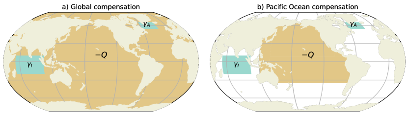
Figure 1: Areas where freshwater flux anomalies are applied with their strengths $\gamma_{A}$ and $\gamma_{I}$; also the global compensation region (a) and the Pacific region (b) is shown.

The procedure to compute bifurcation diagrams of the model, including biases in the freshwater forcing, is the following:

• Under restoring conditions for the surface salinity field Levitus (1994), a steady solution is determined for standard values of the parameters of the model Dijkstra and Weijer (2005). From this steady solution the freshwater flux, below referred to the Levitus flux $F^{L}_{S}$, is diagnosed.

• A freshwater flux over a region near New Foundland (Fig. 1) with domain [$60^{\circ}$ W$,24^{\circ}$ W] $\times$ [$54^{\circ}$ N $,66^{\circ}$ N] is prescribed (in addition to $F^{L}_{S}$) with strength $\gamma_{A}F^{A}_{S}$ Sv, where $F^{A}_{S}=1$ in this domain and zero outside. Similarly, a bias freshwater flux is prescribed over the Indian Ocean domain [$52^{\circ}$ E$,104^{\circ}$ E] $\times$ [$20^{\circ}$ S, $10^{\circ}$ N] with amplitude $\gamma_{I}F^{I}_{S}$ Sv, where $F^{I}_{S}=1$ in this domain and zero outside. The total freshwater flux is prescribed as

  $$F_{S}=F^{L}_{S}+\gamma_{A}F^{A}_{S}+\gamma_{I}F^{I}_{S}-QF^{C}_{S},$$ (4)

  where $F^{C}_{S}=1$ in a compensation domain (specified below) and the quantity $Q$ is determined such that

  $$\int_{S_{oa}}F_{S}~{}r^{2}_{0}\cos\theta~{}d\theta d\phi=0,$$ (5)

  where $S_{oa}$ is the total ocean surface and $r_{0}$ the radius of the Earth.

• In the results below, we will consider two cases of compensation: (a) global compensation, i.e. $C$ is the global ocean domain (Fig. 1a) as in Dijkstra (2007) and (b) $C$ is the Pacific domain (Fig. 1b), so there is no compensation over the Atlantic. In each case, for different (but fixed) values of $\gamma_{I}$, a branch of steady solutions versus $\gamma_{A}$ is calculated under the freshwater forcing (4), starting from the solutions determined under (i) for $\gamma_{A}=\gamma_{I}=0$.

3 Results

In the results below, we concentrate on the bifurcation diagrams and freshwater and salt balances. Plots of the typical AMOC patterns for slightly different parameter values can be found in Dijkstra (2007).

3.1 Global Compensation

The bifurcation diagram for the global compensation case (Fig. 1a) with $\gamma_{I}=0$ (no Indian Ocean freshwater flux bias), where the maximum AMOC strength below 1000 m ($\Psi_{A}$) is plotted versus $\gamma_{A}$ (both in Sv), is shown as the black curve in Fig. 2a.

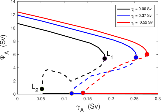
Figure 2: Bifurcation diagrams for the case of global compensation where the maximum strength of the AMOC below 1000 m ($\Psi_{A}$) is plotted versus the strength of the anomalous freshwater forcing $\gamma_{A}$ for different values of $\gamma_{I}$. Drawn (dashed) curves indicate stable (unstable) branches. The dots indicate the saddle-node bifurcations.

With increasing $\gamma_{A}$, stable (black drawn curves) steady states exist for which the AMOC strength decreases and at $\gamma^{1}_{A}=0.186$ Sv, a first saddle-node bifurcation $L_{1}$ occurs. With decreasing $\gamma_{A}$, a branch of unstable steady states (black dashed curves) exists down to a second saddle-node bifurcation $L_{2}$ at $\gamma^{2}_{A}=0.054$ Sv.

The width of the multi-stable regime, often called the hysteresis width $\Delta_{H}$, is given by

$$\Delta_{H}=|\gamma^{1}_{A}-\gamma^{2}_{A}|.$$ (6)

For the case $\gamma_{I}=0$, we find $\Delta_{H}=0.132$ Sv in this model. In typical quasi-equilibrium model studies Rahmstorf et al. (2005), where $\gamma_{A}$ is varied with about 0.05 Sv/1000 years, the width is typically overestimated. With continuation methods, as used here, one is able to determine the hysteresis width very accurately as the values of $\gamma^{1,2}_{A}$ are computed explicitly.

With increasing values of $\gamma_{I}$ (adding fresh water over the Indian Ocean) both saddle node-bifurcations $L_{1}$ and $L_{2}$ move to larger values of $\gamma_{A}$ (Fig. 2) indicating that the multi-stable regime occurs for higher Atlantic freshwater forcing. Hence, with the Indian Ocean freshwater flux bias, it is less likely that GCM having a ‘Levitus-like’ surface salinity are in a multi-stable regime (than models without such a bias). The width of the multi-stable regime versus $\gamma_{I}$ does not change much for these $\gamma_{I}$ values; $\Delta_{H}=0.137$ Sv and $\Delta_{H}=0.138$ Sv are found for $\gamma_{I}=0.37$ Sv and $\gamma_{I}=0.52$ Sv, respectively.

To understand the shift of the branches in the bifurcation diagram, we consider the Atlantic freshwater transport by the AMOC and the gyres. Following De Vries and Weber (2005), the quantities $F_{ov}$ (the overturning component) and $F_{az}$ (the azonal component) are computed as

$$F_{ov}(\theta)&=-\frac{r_{0}}{S_{0}}\int_{S_{\theta}}\bar{v}(<S>-S_{0})~{}dz~{};\\ F_{az}(\theta)=-\frac{r_{0}}{S_{0}}\int_{S_{\theta}}\overline{v^{\prime}S^{\prime}}~{}dz.$$ (7)

where $S_{0}=35$ psu is a reference salinity, $r_{0}$ is the radius of the Earth, and $S_{\theta}$ is the boundary (longitude, depth) at latitude $\theta$. Here, the quantities $\bar{v}$, $\bar{S}$, $<v>$ and $<S>$ are given by

$$\bar{v}&=\int v\cos\theta~{}d\phi~{};~{}<v>=\frac{\bar{v}}{\int\cos\theta~{}d\phi},\\ \bar{S}=\int S\cos\theta~{}d\phi~{};~{}<S>=\frac{\bar{S}}{\int\cos\theta~{}d\phi},$$ (8)

and $v^{\prime}=v-<v>$ and $S^{\prime}=S-<S>$. The physical meaning of these quantities is extensively discussed in De Vries and Weber (2005) and Dijkstra (2007).

The existence of the saddle-node bifurcations $L_{1}$ and $L_{2}$ can be connected to the behavior of $F_{ovS}$. In simple box models Cessi (1994); Rahmstorf (1996), the saddle-node bifurcation $L_{1}$ at $\gamma^{1}_{A}$ is related to a minimum in $F_{ovS}$. In our model, this is more complicated as there is also a gyre-driven freshwater transport, and the $F_{ovS}$ minimum is only approximate. The saddle-node bifurcation $L_{2}$ at $\gamma^{2}_{A}$ near to a zero of $F_{ovS}$ along the upper branch of the AMOC, as discussed at length in Dijkstra (2007). So to explain the shift in positions in the saddle-node bifurcations we focus on the behaviour of $F_{ovS}$, $F_{ovN}$ while also monitoring their difference $\Delta F_{ov}=F_{ovS}-F_{ovN}$ and the associated behaviour of the freshwater transports by the gyres.

The results for $F_{ovS}=F_{ov}(35^{\circ}$S), $F_{ovN}=F_{ov}(60^{\circ}$N) and $\Delta F_{ov}$ are shown in Fig. 3a, with the case $\gamma_{I}=0$ ($\gamma_{I}=0.37$ Sv) as drawn (dashed) curves.

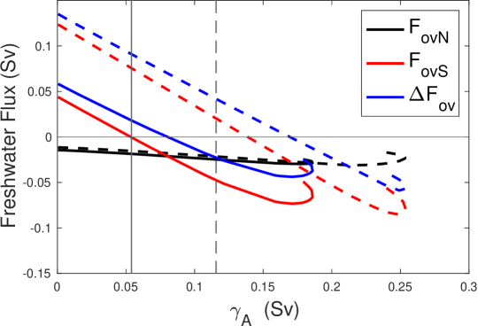
(a)

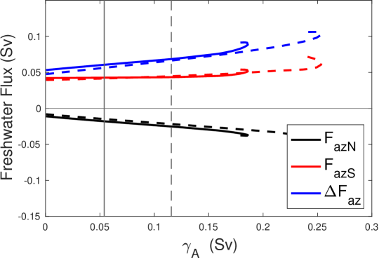
(b)

Figure 3: Global compensation case. (a) Values of the AMOC induced freshwater transport at the southern boundary (35^∘S) of the Atlantic ($F_{ovS}$), the northern boundary (60^∘N) of the Atlantic ($F_{ovN}$), and their difference $\Delta F_{ov}$. (b) Same as (a) but for the azonal transport ($F_{azS}$, $F_{azN}$ and $\Delta F_{az}$). The drawn curves are for $\gamma_{I}=0$, corresponding to the black curve in Fig. 2. The dashed curves are for $\gamma_{I}=0.37$ Sv, corresponding to the blue curve in Fig. 2.

For the chosen northern latitude (60^∘N), the freshwater flux $F_{ovN}$ is negative and the AMOC transports freshwater southwards for all values of $\gamma_{A}$. For $\gamma_{A}=0$, the AMOC transports freshwater northwards at 35^∘S as $F_{ovS}>0$. With increasing $\gamma_{A}$, $F_{ovS}$ decreases and, for $\gamma_{I}=0$, becomes negative close to the saddle-node bifurcation $L_{2}$ at $\gamma^{2}_{A}$ (indicated by the thin drawn vertical line). For $\gamma_{I}=0.37$ Sv, the value of $F_{ovS}$ at $\gamma_{A}=0$ is much larger (than that for $\gamma_{I}=0$). Because $F_{ovS}$ decreases with $\gamma_{A}$ at the same rate as for $\gamma_{I}=0$, the location where $F_{ovS}\approx 0$ and hence the bifurcation $\gamma^{2}_{A}$ occurs at a larger value of $\gamma_{A}$. Also the location where $F_{ovS}$ obtains its minimum, and hence the position of $L_{1}$ (at $\gamma^{1}_{A}$) shifts to the right. The gyre transport changes $F_{azS}$, $F_{azN}$ and $\Delta F_{az}$ with $\gamma_{A}$ are shown in Fig. 3b and do not change much with $\gamma_{I}$.

As shown in Dijkstra (2007), the fully-implicit model allows for a closed salt balance over the Atlantic from $\theta_{s}=35^{\circ}$S to $\theta_{n}=60^{\circ}$N from which changes in advective, diffusive and surface contributions can be determined. The terms in this balance are shown in Fig. 4 for both cases $\gamma_{I}=0$ and $\gamma_{I}=0.37$ Sv. Expressions for these terms were presented in Dijkstra (2007), but are repeated here for convenience, i.e.

$$\Phi^{s}&=\int_{S_{oa}}S_{0}F_{S}~{}r^{2}_{0}\cos\theta~{}d\phi d\theta,\\ \Phi^{a}(\theta)=-\int_{S_{\theta}}vS~{}r_{0}\cos\theta~{}d\phi dz,\\ \Phi^{d}(\theta)=\int_{S_{\theta}}K_{H}\frac{\partial S}{\partial\theta}~{}\cos\theta~{}d\phi dz,$$ (9)

where $\Phi^{a}$ and $\Phi^{d}$ are the advective and diffusive fluxes through the boundary $S_{\theta}$, respectively. The overall balance is given by

$$\Phi^{b}=\Phi^{a}(\theta_{n})-\Phi^{d}(\theta_{n})-\Phi^{a}(\theta_{s})+\Phi^{d}(\theta_{s})-\Phi^{s}$$ (10)

Indeed, the term $\Phi^{b}$ is much smaller than the individual terms (black curves in Fig. 4) giving a nearly closed salt balance over the Atlantic basin for all values of the parameters.

First consider the case $\gamma_{I}=0$ (drawn curves in Fig. 4) and the upper branch in the bifurcation diagram up to $L_{1}$. For $\gamma_{A}=0$, the surface (virtual) salt flux is approximately balanced by the fluxes at the southern boundary. The surface evaporation is larger than the precipitation ($\Phi^{s}>0$) and this salt is transported out of the Atlantic basin at the southern boundary ($\Phi^{a}(\theta_{s})<0$). The fact that the diffusive flux is relatively large here (compared to typical GCMs) is that the model has a coarse resolution so needs a relatively high horizontal diffusivity to prevent wiggles to occur near the boundaries. The salt fluxes at the northern boundary are less important and the respective components are about a factor 2 to 4 smaller than at the southern boundary.

With increasing $\gamma_{A}$, the surface salt flux decreases as freshwater is put into the North Atlantic. The diffusive salt transports do not respond but the southward advective salt transport at $\theta_{s}$ weakens and eventually changes sign near $\gamma_{A}=0.1$ Sv. As the diffusive flux is directed to transport salt into the basin at the southern boundary, the value of $\gamma_{A}$ where the sign change in salt transport occurs is around $0.06$ Sv (Fig. 4). Note that the gyre and AMOC components cannot be distinguished in the advective fluxes.

When $\gamma_{I}=0.37$ Sv (dashed curves in Fig. 4), the surface salt flux increases for $\gamma_{A}=0$ compared to the case $\gamma_{I}=0$. This is due to the global compensation as a negative salt flux in the Indian Ocean is compensated by a positive one over part of the Atlantic. Hence, the curve for $\Phi^{s}$ shifts upwards and so the compensating advective flux at the southern boundary shifts downwards. A second effect is that the changed surface freshwater flux pattern leads to a modified salinity distribution in the Atlantic. This increases the AMOC (Fig. 2) strength and hence also its salt transport out of the basin at the southern boundary.

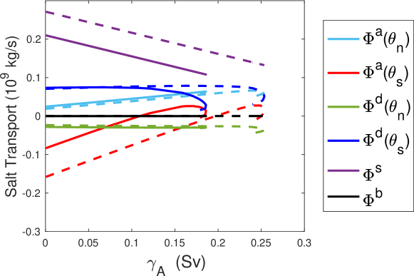
Figure 4: Global compensation case. Terms in the integrated salt balance (given in Sv) over the Atlantic basin over the upper branches in Fig. 2 (up to $\gamma^{1}_{A}$), with expressions of the terms as indicated in (9) and (10) for $\theta_{n}=60^{\circ}$N and $\theta_{s}=35^{\circ}$S. The drawn curves are for the case $\gamma_{I}=0$ and the dashed ones for $\gamma_{I}=0.37$ Sv.

Because the diffusive fluxes are not much affected by the Indian Ocean freshwater input, the fluxes $\Phi^{s}$ and $\Phi^{a}(\theta_{s})$ change with $\gamma_{A}$ in the same way as for the case $\gamma_{I}=0$. The starting value of $\Phi^{s}$ at $\gamma_{A}=0$ is now larger and it takes a larger value of $\gamma_{A}$ to change the sign of the freshwater flux at the southern boundary and to reach a minimum in this quantity. Hence the saddle-node bifurcations $L_{1}$ and $L_{2}$ shifts to larger values of $\gamma_{A}$.

3.2 Pacific Compensation

Since the global compensation has a substantial influence on the position of the saddle-node bifurcations (Fig. 2), we now consider the case where compensation is only over the Pacific domain as indicated in Fig. 1b. The bifurcation diagrams in this case are, for different values of $\gamma_{I}$, shown in Fig. 5. The shift of the saddle-nodes to larger values of $\gamma_{A}$ is much smaller than for the global compensation case (Fig. 2). The hysteresis width itself for $\gamma_{I}=0$ with $\Delta_{H}=0.103$ Sv for the Pacific compensation case is a bit smaller than for the global compensation case ($\Delta_{H}=0.138$ Sv). This width is only slightly larger for the case $\gamma_{I}=0.52$ Sv, i.e. $\Delta_{H}=0.111$ Sv.

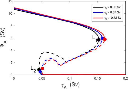
Figure 5: Bifurcation diagram for the case of Pacific compensation where the maximum strength of the AMOC below 1000 m ($\Psi_{A}$) is plotted versus the strength of the anomalous Atlantic freshwater forcing $\gamma_{A}$ for different values of $\gamma_{I}$. The dots indicate the saddle-node bifurcations.

For the analysis of the freshwater and salt balances, we choose the larger value ($\gamma_{I}=0.52$ Sv) instead of $\gamma_{I}=0.37$ Sv (used in the global compensation case), as the differences are more clearly visible. The freshwater transports by the AMOC and by the gyres (Fig. 6) show that for $\gamma_{A}=0$, $F_{ov}$ is larger for $\gamma_{I}=0.52$ Sv (Fig. 6a), compared to the case $\gamma_{I}=0.0$ Sv. Hence also changes in the freshwater balance are induced in the Atlantic, but both the direct effect of compensation of the surface freshwater flux and the secondary effect of an AMOC increase are much smaller. Of course, in such a diffusive and viscous model, the Agulhas retroflection is in a diffusive retroflection regime Dijkstra and De Ruijter (2001) but there is additional freshwater transport from the Indian to the Atlantic when $\gamma_{I}>0$. As the wind-driven freshwater transport does not change much with $\gamma_{A}$ (Fig. 6b), the AMOC transports more freshwater into the basin and hence $F_{ovS}$ becomes more positive.

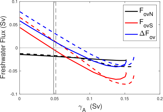
(a)

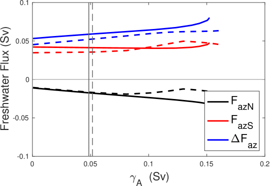
(b)

Figure 6: Pacific compensation case. (a) Values of the AMOC induced freshwater transport at the southern boundary (35^∘S) of the Atlantic ($F_{ovS}$), the northern boundary (60^∘N) of the Atlantic ($F_{ovN}$), and their difference ($\Delta F_{ov}$). (b) Same as (a) but for the azonal transport ($F_{azS}$, $F_{azN}$ and $\Delta F_{az}$). The drawn curves are for $\gamma_{I}=0$, corresponding to the black curve in Fig. 5. The dashed curves are for $\gamma_{I}=0.52$ Sv, corresponding to the red curves in Fig. 5.

In the Atlantic salt balance (Fig. 7) the surface salt flux is indeed the same for both values of $\gamma_{I}$, because there is no compensation anymore over the Atlantic. The advective transport of salt becomes slightly more negative over the southern boundary for $\gamma_{I}=0.52$ Sv indicating that indeed a small amount of freshwater is transported into the Atlantic basin. Also the diffusive transport of salt (into the basin) decreases and this approximately balances the advective contribution. As the advective contribution is much smaller than the compensation contribution in the global compensation case, the shift of the saddle-node bifurcations to larger values of $\gamma_{A}$ is much smaller.

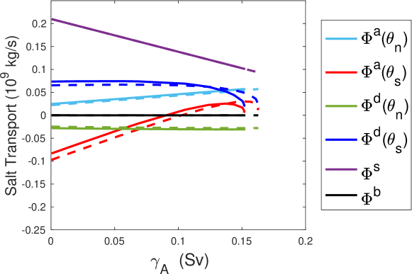
Figure 7: Pacific compensation case. Terms in the integrated salt balance over the Atlantic basin over the upper branch in Fig. 5, with expressions of the terms as indicated in the main text. The drawn curves are for the case $\gamma_{I}=0$ and the dashed ones for $\gamma_{I}=0.52$ Sv.

4 Summary and Discussion

Following earlier studies on CMIP3 and CMIP5 models Drijfhout et al. (2013); Mecking et al. (2016), also many CMIP6 models have large biases in surface freshwater fluxes which lead to an AMOC with an Atlantic freshwater transport that is in disagreement with observations van Westen and Dijkstra (2023). The most important model bias is in the Atlantic Surface Water properties, which arises from deficiencies in the surface freshwater flux over the Indian Ocean. A second bias is in the properties in the North Atlantic Deep Water and arises through deficiencies in the freshwater flux over the Atlantic Subpolar Gyre region van Westen and Dijkstra (2023).

In this paper, we have addressed to effects of the freshwater flux bias in the Indian Ocean on the multiple equilibrium regime of the AMOC using the fully implicit global ocean-atmosphere model of Dijkstra and Weijer (2005), for which explicit bifurcation diagrams can be computed. This is a fantastic capability as both stable and unstable steady states can be computed, and the width of the multiple equilibrium regime can be determined accurately. However, this can only be done with quite a simplified global model, with relatively low resolution and hence being more viscous and diffusive than current, even low-resolution, ocean models. The atmosphere model is only an energy balance model with a prescribed freshwater forcing. In terms of quantitative results on changes of the bifurcation diagrams, the model is probably not that useful.

Qualitatively, however, the model provides very useful information, as it indicates that the multiple equilibrium regime does not disappear due to the Indian Ocean freshwater flux biases, but that it shifts to higher values of the North Atlantic anomalous freshwater flux. This shift is dependent on the way the latter flux is compensated. There are two mechanisms which are responsible for these shifts: surface salinity patterns in the Atlantic depend on the compensation of the Indian Ocean bias and, in both cases considered here, lead to a slight increase in the AMOC. In the Levitus background state (with $F_{ovS}>0$), this leads to a larger transport of salt out of the Atlantic basin. Hence, a larger anomalous North Atlantic surface freshwater flux is needed to activate the salt advection feedback, i.e., to a situation where the AMOC exports fresh water. When there is compensation of the Indian Ocean freshwater flux in the Atlantic, the Atlantic becomes saltier and hence the AMOC transports more salt out of the basin. This leads to an additional, and here larger, shift of the bifurcation diagram compared to when there is no compensation in the Atlantic.

The mechanisms identified are useful for interpreting results from GCMs and for designing new simulations with these models. First it shows that biases in freshwater flux lead to shifts in the bifurcation diagram which would imply that such multiple equilibrium regimes (and hence AMOC collapses) could exist in these models but are located in a parameter regime where one would not normally perform simulations. Second, it provides a hint why efforts to find AMOC collapses in these models may not have been successful Mecking et al. (2016); Jackson and Wood (2018b, a). Even an enormous freshwater input in a parameter regime which is outside the multiple equilibrium regime would only lead to a weakened (but no collapsed) AMOC.

This also suggests several ways forward to find an AMOC collapse in state-of-the-art models. One either performs a long quasi-equilibrium simulation up to very large freshwater flux input such as in the FAMOUS model Hawkins et al. (2011) to find the collapse (this may take a few thousand years of simulation, so is expensive). In doing this, it is better to compensate outside of the Atlantic when using surface fluxes, as the latter will introduce an additional shift and so one has to integrate longer to find an AMOC collapse. Such compensation procedures (including compensation over the volume) are now also more common in GCMs Jackson et al. (2022). The alternative is to address and improve the biases in the atmospheric components of the models, but this is not an easy issue. The origin of these biases may even be a coupled problem, as the bias strength is positively correlated with the AMOC strength van Westen and Dijkstra (2023).

We hope that this study will motivate the design of new AMOC hosing simulations to find AMOC collapses in state-of-the-art GCMs. Detection of such a collapse would have a large impact on climate change research and probability estimates of AMOC tipping under global warming would likely need to be revised.

Acknowledgements

H.A.D. and R.M.v.W. are funded by the European Research Council through the ERC-AdG project TAOC (project 101055096). The authors thank Dr. Fred Wubs (University of Groningen, NL) for helping with revising the old Fortran code of the model Dijkstra (2007) used in this paper.

References

- Armstrong McKay et al. (2022) Armstrong McKay, D. I., Staal, A., Abrams, J. F., Winkelmann, R., Sakschewski, B., Loriani, S., Fetzer, I., Cornell, S. E., Rockström, J., and Lenton, T. M. (2022). Exceeding 1.5 C global warming could trigger multiple climate tipping points. Science, 377(6611), eabn7950.
- Bryan and Lewis (1979) Bryan, K. and Lewis, L. J. (1979). A water mass model of the world ocean. J. Geophys. Res., 84, 2503–2517.
- Bryden et al. (2011) Bryden, H. L., King, B. A., and McCarthy, G. D. (2011). South Atlantic overturning circulation at 24S. Journal of Marine Research, 69, 38–55.
- Cessi (1994) Cessi, P. (1994). A simple box model of stochastically forced thermohaline flow. J. Phys. Oceanogr., 24, 1911–1920.
- Cimatoribus et al. (2012) Cimatoribus, A., Drijfhout, S., Toom, M., and Dijkstra, H. (2012). Sensitivity of the Atlantic meridional overturning circulation to South Atlantic freshwater anomalies. Climate Dynamics, 39, 2291 – 2306.
- De Niet et al. (2007) De Niet, A., Wubs, F., van Scheltinga, A. T., and Dijkstra, H. A. (2007). A tailored solver for bifurcation analysis of ocean-climate models. Journal of Computational Physics, 227(1), 654–679.
- De Vries and Weber (2005) De Vries, P. and Weber, S. L. (2005). The Atlantic freshwater budget as a diagnostic for the existence of a stable shut down of the meridional overturning circulation. Geophys. Res. Letters, 32, L09606.
- Dijkstra (2005) Dijkstra, H. A. (2005). Nonlinear Physical Oceanography: A Dynamical Systems Approach to the Large Scale Ocean Circulation and El Niño, 2nd Revised and Enlarged edition. Springer, New York, 532 pp.
- Dijkstra (2007) Dijkstra, H. A. (2007). Characterization of the multiple equilibria regime in a global ocean model. Tellus, 59A, 695–705.
- Dijkstra and De Ruijter (2001) Dijkstra, H. A. and De Ruijter, W. P. M. (2001). On the physics of the Agulhas current: Steady retroflection regimes. J. Phys. Oceanogr., 31, 2971–2985.
- Dijkstra and Weijer (2005) Dijkstra, H. A. and Weijer, W. (2005). Stability of the global ocean circulation: basic bifurcation diagrams. J. Phys. Oceanogr., 35, 933–948.
- Drijfhout et al. (2013) Drijfhout, S., Gleeson, E., Dijkstra, H. A., and Levina, V. (2013). Spontaneous abrupt climate change due to an atmospheric blocking– sea-ice–ocean feedback in an unforced climate model simulation. Proceedings National Acad. Sciences.
- England (1993) England, M. H. (1993). Representing the global-scale water masses in ocean general circulations models. J. Phys. Oceanogr., 23, 1523–1552.
- Gent (2018) Gent, P. R. (2018). A commentary on the atlantic meridional overturning circulation stability in climate models. Ocean Modelling, 122, 57–66.
- Hawkins et al. (2011) Hawkins, E., Smith, R. S., Allison, L. C., Gregory, J. M., Woollings, T. J., Pohlmann, H., and De Cuevas, B. (2011). Bistability of the Atlantic overturning circulation in a global climate model and links to ocean freshwater transport. Geophysical Research Letters, 38(10), L10605.
- Hu et al. (2012) Hu, A., Meehl, G. A., Han, W., Timmermann, A., Otto-Bliesner, B., Liu, Z., Washington, W. M., Large, W., Abe-Ouchi, A., Kimoto, M., Lambeck, K., and Wu, B. (2012). Role of the Bering Strait on the hysteresis of the ocean conveyor belt circulation and glacial climate stability. Proceedings of the National Academy of Sciences, 109(17), 6417–6422.
- Huisman et al. (2010) Huisman, S. E., den Toom, M., Dijkstra, H. A., and Drijfhout, S. (2010). An Indicator of the Multiple Equilibria Regime of the Atlantic Meridional Overturning Circulation. Journal Of Physical Oceanography, 40(3), 551–567.
- Jackson and Wood (2018a) Jackson, L. C. and Wood, R. A. (2018a). Hysteresis and Resilience of the AMOC in an Eddy‐Permitting GCM. Geophysical Research Letters, 45(16), 8547 – 8556.
- Jackson and Wood (2018b) Jackson, L. C. and Wood, R. A. (2018b). Timescales of AMOC decline in response to fresh water forcing. Climate Dynamics, 51(4), 1333 – 1350.
- Jackson et al. (2015) Jackson, L. C., Kahana, R., Graham, T., Ringer, M. A., Woollings, T., Mecking, J. V., and Wood, R. A. (2015). Global and European climate impacts of a slowdown of the AMOC in a high resolution GCM. Climate Dynamics, 45(11), 3299 – 3316.
- Jackson et al. (2022) Jackson, L. C., Asenjo, E. A. d., Bellomo, K., Danabasoglu, G., Haak, H., Hu, A., Jungclaus, J., Lee, W., Meccia, V. L., Saenko, O., Shao, A., and Swingedouw, D. (2022). Understanding AMOC stability: the North Atlantic Hosing Model Intercomparison Project. Geoscientific Model Development Discussions, 2022, 1–32.
- Keller (1977) Keller, H. B. (1977). Numerical solution of bifurcation and nonlinear eigenvalue problems. In P. H. Rabinowitz, editor, Applications of Bifurcation Theory. Academic Press, New York, U.S.A.
- Lenton et al. (2008) Lenton, T. M., Held, H., Kriegler, E., Hall, J. W., Lucht, W., Rahmstorf, S., and Schellnhuber, H. J. (2008). Tipping elements in the Earth’s climate system. Proceedings of the National Academy of Sciences of the United States of America, 105(6), 1786–93.
- Levitus (1994) Levitus, S. (1994). World Ocean Atlas 1994, Volume 4: Temperature. NOAA/NESDIS E, US Department of Commerce, Washington DC, OC21, 1–117.
- Liu et al. (2017) Liu, W., Xie, S.-P., Liu, Z., and Zhu, J. (2017). Overlooked possibility of a collapsed Atlantic Meridional Overturning Circulation in warming climate. Science Advances, 3(1), e1601666.
- Liu et al. (2020) Liu, W., Fedorov, A. V., Xie, S.-P., and Hu, S. (2020). Climate impacts of a weakened Atlantic Meridional Overturning Circulation in a warming climate. Science Advances, 6(26), eaaz4876.
- Lohmann et al. (2021) Lohmann, J., Castellana, D., Ditlevsen, P. D., and Dijkstra, H. A. (2021). Abrupt climate change as rate-dependent cascading tipping point. Earth System Dynamics Discussions, 2021, 1–25.
- Marotzke (2000) Marotzke, J. (2000). Abrupt climate change and thermohaline circulation: Mechanisms and predictability. Proc. Natl. Acad. Sci., 97, 1347–1350.
- Mecking et al. (2016) Mecking, J. V., Drijfhout, S. S., Jackson, L. C., and Graham, T. (2016). Stable AMOC off state in an eddy-permitting coupled climate model. Climate Dynamics, 47(7), 2455 – 2470.
- Mulder et al. (2021) Mulder, T. E., Goelzer, H., Wubs, F. W., and Dijkstra, H. A. (2021). Snowball Earth Bifurcations in a Fully-Implicit Earth System Model. International Journal of Bifurcation and Chaos, 31(06), 2130017.
- Orihuela-Pinto et al. (2022) Orihuela-Pinto, B., England, M. H., and Taschetto, A. S. (2022). Interbasin and interhemispheric impacts of a collapsed atlantic overturning circulation. Nature Climate Change, 12(6), 558–565.
- Rahmstorf (1996) Rahmstorf, S. (1996). On the freshwater forcing and transport of the Atlantic thermohaline circulation. Climate Dynamics, 12(12), 799–811.
- Rahmstorf et al. (2005) Rahmstorf, S., Crucifix, M., Ganopolski, A., Goosse, H., Kamenkovich, I., Knutti, R., Lohmann, G., March, R., Mysak, L., Wang, Z., and Weaver, A. J. (2005). Thermohaline circulation hysteresis: a model intercomparison. Geophys. Res. Letters, L23605, doi:0.1029/2005GLO23655, 1–5.
- Stommel (1961) Stommel, H. (1961). Thermohaline convection with two stable regimes of flow. Tellus, 2, 244–230.
- Stouffer et al. (2006) Stouffer, R. J., Yin, J., Gregory, J. M., Dixon, K. W., Spelman, M. J., Hurlin, W., Weaver, A. J., Eby, M., Flato, G. M., Hasumi, H., Hu, A., Jungclaus, J. H., Kamenkovich, I. V., Levermann, A., Montoya, M., Murakami, S., Nawrath, S., Oka, A., Peltier, W. R., Robitaille, D. Y., Sokolov, A. P., Vettoretti, G., and Weber, S. L. (2006). Investigating the causes of the response of the thermohaline circulation to past and future climate changes. Journal of Climate, 19, 1365–1387.
- Toom et al. (2012) Toom, M. D., Dijkstra, H. a., Cimatoribus, A. a., and Drijfhout, S. S. (2012). Effect of Atmospheric Feedbacks on the Stability of the Atlantic Meridional Overturning Circulation. Journal of Climate, 25(12), 4081–4096.
- Trenberth et al. (1989) Trenberth, K. E., Olson, J. G., and Large, W. G. (1989). A global ocean wind stress climatology based on ECMWF analyses. Technical report, National Center for Atmospheric Research, Boulder, CO, U.S.A.
- van Westen and Dijkstra (2023) van Westen, R. M. and Dijkstra, H. A. (2023). Persistent Climate Model Biases in the Atlantic Ocean’s Freshwater Transport. Ocean Science Discussions. submitted.
- Vellinga et al. (2002) Vellinga, M., Wood, R. A., and Gregory, J. M. (2002). Processes governing the recovery of a perturbed thermohaline circulation in HadCM3. J. Climate, 15, 764–780.
- Weijer et al. (2019) Weijer, W., Cheng, W., Drijfhout, S. S., Fedorov, A. V., Hu, A., Jackson, L. C., Liu, W., McDonagh, E. L., Mecking, J. V., and Zhang, J. (2019). Stability of the Atlantic Meridional Overturning Circulation: A Review and Synthesis. Journal Of Geophysical Research-Oceans, 124(8), 5336 – 5375.