Internal Cross-layer Gradients for Extending Homogeneity to Heterogeneity in Federated Learning

Abstract

Federated learning (FL) inevitably confronts the challenge of system heterogeneity in practical scenarios. To enhance the capabilities of most model-homogeneous FL methods in handling system heterogeneity, we propose a training scheme that can extend their capabilities to cope with this challenge. In this paper, we commence our study with a detailed exploration of homogeneous and heterogeneous FL settings and discover three key observations: (1) a positive correlation between client performance and layer similarities, (2) higher similarities in the shallow layers in contrast to the deep layers, and (3) the smoother gradients distributions indicate the higher layer similarities. Building upon these observations, we propose InCo Aggregation that leverags internal cross-layer gradients, a mixture of gradients from shallow and deep layers within a server model, to augment the similarity in the deep layers without requiring additional communication between clients. Furthermore, our methods can be tailored to accommodate model-homogeneous FL methods such as FedAvg, FedProx, FedNova, Scaffold, and MOON, to expand their capabilities to handle the system heterogeneity. Copious experimental results validate the effectiveness of InCo Aggregation, spotlighting internal cross-layer gradients as a promising avenue to enhance the performance in heterogenous FL.

1 Introduction

Federated learning (FL) is proposed to enable a federation of clients to effectively cooperate towards a global objective without exchanging raw data mcmahan2017communication . While FL makes it possible to fuse knowledge in a federation with privacy guarantees huang2021evaluating ; mcmahan2017communication ; jeong2022factorized , its inherent attribute of system heterogeneity, e.g., varying computation and communication resources, may hinder the training process and even lower the quality of the jointly-learned models kairouz2019advances ; li2020federated ; mohri2019agnostic ; Survey_on_Heterogeneous .

Existing works cater to system heterogeneity by aligning the local models of varying architectures (i.e., model heterogeneity) to make full use of local resources diao2021heterofl ; baek2022joint ; alamfedrolex ; huang2022learn ; fang2022robust ; lin2020ensemble . Heterogeneous devices are allocated to a common model prototype tailored to their varying sizes, such as ResNets with different depths or widths of layers liu2022no ; diao2021heterofl ; horvath2021fjord ; baek2022joint ; caldas2018expanding , strides of layers tan2022fedproto , or numbers of kernels alamfedrolex , to account for their inherent resource constraints. It is worth mentioning that heterogeneous FL refers to the settings of heterogeneous data distributions and model architectures. While several methods have been proposed to incorporate heterogeneous models into federated learning (FL), their performance often falls short compared to FL training using homogeneous models of the same size he2020group ; diao2021heterofl . Therefore, gaining a comprehensive understanding of the factors that limit the performance of heterogeneous models in FL is imperative. The primary objective of this paper is to investigate the underlying reasons behind this limitation and propose a potential solution that acts as a bridge between model homogeneity and heterogeneity to tackle this challenge.

In light of this, we first conduct a case study to reveal the obstacles affecting the performance of heterogeneous models in FL. The observations from this case study are enlightening: (1) With increasing heterogeneity in data distributions and model architectures, we observe a decline in model accuracy and layer-wise similarity (layer similarity) as measured by Centered Kernel Alignment (CKA) kornblith2019similarity , a quantitative metric of bias luo2021no ; raghu2021vision ; (2) The deeper layers share lower layer similarity across the clients, while the shallower layers exhibit greater alignment. These insights further shed light on the intriguing notion that shallow layers possess the ability to capture shared features across diverse clients, even within the heterogeneous FL setting. Moreover, these observations indicate that the inferior performances in heterogeneous FL are related to the lower similarity in the deeper layers. Motivated by these compelling findings, we come up with an idea: Can we enhance the similarity of deeper layers, thereby attaining improved performance?

To answer this question, we narrow our focus to the gradients, as the dissimilarity of deep layers across clients is a direct result of gradient updates ruder2016overview ; chen2021communication . Interestingly, we observe that (3) the gradient distributions emanating from shallow layers are smoother and possess higher similarity than those from deep layers, establishing a connection between the gradients and the layer similarity. Therefore, inspired by these insights, we propose a method called InCo Aggregation, where a server model utilizes the Internal Cross-layer gradients (InCo) to improve the similarity of its deeper layers without additional communications with the clients. More specifically, cross-layer gradients are mixtures of the gradients from the shallow and the deep layers. We utilize cross-layer gradients as internal knowledge, effectively transferring knowledge from the shallow layers to the deep layers. Nevertheless, mixing these gradients directly poses a significant challenge called gradient divergence wang2020tackling ; zhao2018federated . To tackle this issue, we normalize the cross-layer gradients and formulate a convex optimization problem that rectifies their directions and obtain its analytic solution. In this way, InCo Aggregation automatically assigns optimal weights to the cross-layer gradients, thus avoiding labor-intensive parameter tuning. Furthermore, InCo Aggregation can extend to model-homogeneous FL methods that previously do not support model heterogeneity, such as FedAvgmcmahan2017communication , FedProx li2018federated , FedNova wang2020tackling , Scaffold karimireddy2020scaffold , and MOON li2021model , to develop their abilities in managing the model heterogeneity problem.

Our main contributions are summarized as follows:

• We first conduct a case study on homogeneous and heterogeneous FL settings and find that (1) client performance is positively correlated to layer similarities across different client models, (2) similarities in the shallow layers are higher than the deep layers, and (3) smoother gradient distributions hint for higher layer similarities.

• We propose InCo Aggregation, applying the internal cross-layer gradients inside a server model. Moreover, our methods can be seamlessly applied to various model-homogeneous FL methods, equipping them with the ability to handle model heterogeneity.

• We establish the non-convex convergence of utilizing cross-layer gradients in FL and derive the convergence rate.

• Extensive experiments validate the effectiveness of InCo Aggregation, showcasing its efficacy in strengthening model-homogeneous FL methods for heterogeneous FL scenarios.

2 Preliminary

To investigate the performance of clients in diverse federated learning settings, we present a case study encompassing both homogeneous and heterogeneous model architectures with CIFAR-10 and split data based on IID and Non-IID based on ResNets he2016identity and ViTs dosovitskiy2020image . We use CKA kornblith2019similarity similarities among models to measure the extent of bias exhibited by each model. We describe the key findings below. More detailed results of the case study are provided in Appendix E.

2.1 A Case Study in Different Federated Learning Environments

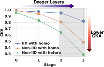
(a) The CKA similarity of ResNets.

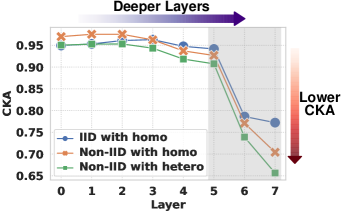
(b) The CKA similarity of ViTs.

Figure 1: The CKA similarity of different federated settings. The purple arrow indicates the direction of the deeper layers, and the red arrow signifies the direction of lower similarity.

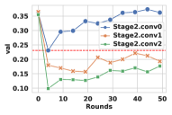
(a) Similarity of gradients in Stage 2.

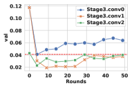
(b) Similarity of gradients in Stage 3.

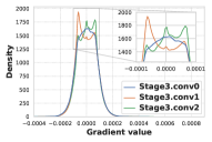
(c) Gradient distributions in Non-IID with hetero.

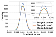
(d) Gradient distributions in IID with homo.

Figure 2: Cross-environment similarity and gradients distributions. (a) and (b): Similarity from Stage 2 and Stage 3. (c) and (d): The gradient distributions of Non-IID with hetero and IID with homo.

Case Analysis. As depicted in Table 1, the performance gap between the most challenging Non-IID with hetero setting and the IID with homo setting is substantial (28.7% in ResNets and 28% in ViTs).

Table 1: Accuracy of the case study.

Settings		Test Accuracy
ResNet	IID with homo	81.0
	Non-IID with homo	62.3($\downarrow$18.7)
	Non-IID with hetero	52.3($\downarrow$28.7)
ViT	IID with homo	81.0
	Non-IID with homo	54.8($\downarrow$26.2)
	Non-IID with hetero	53.0($\downarrow$28.0)

Furthermore, Figure 1 illustrates that the CKA similarity among the deeper layers consistently decreases compared to the shallower layers, with a noticeable decline highlighted in the gray area. Generally, we find two intriguing observations from Table 1 and Figure 1: (i) The deeper layers or stages have lower CKA similarities than the shallow layers. (ii) The settings with higher accuracy also obtain higher CKA similarities in the deeper layers or stages. These observations indicate that increasing the similarity of deeper layers can serve as a viable approach to improving client performance. Considering that shallower layers exhibit higher similarity, a potential direction emerges: to improve the CKA similarity in deeper layers according to the knowledge from the shallower layers.

2.2 Deep Insights of Gradients in the Shallower Layers

Gradients as Knowledge. Based on the insights gleaned from the previous case study, it is evident that knowledge extracted from the shallow layers exhibits higher similarity. In FL, there are two primary types of knowledge that can be utilized: features, which are outputs from corresponding middle layers, and gradients from respective layers. We intentionally choose to use gradients as our primary knowledge for two essential reasons. Firstly, our FL environment lacks a shared dataset, impeding the establishment of a connection between different clients using features derived from the same data. Secondly, utilizing features in FL would significantly increase communication overheads. Hence, taking these practical considerations into account, we select gradients as the knowledge derived from the shallow layers.

Cross-environment Similarity. In this subsection, we deeply investigate the cross-environment similarity of ResNet gradients between two environments, i.e., IID with homo and Non-IID with hetero, to shed light on the disparities between shallow and deep layers in the same stage and identify the gaps between the homogeneous and heterogeneous FL. As depicted in Figure 2a and 2b, gradients from shallow layers (Stage2.conv0 and Stage3.conv0) exhibit higher cross-environment CKA similarity than those from deep layers such as Stage2.conv1, and Stage3.conv2. Notably, even the lowest similarities (red lines) in Stage2.conv0 and Stage3.conv0 surpass the highest similarities in deep layers. These findings underscore the superior quality of gradients obtained from shallow layers relative to those obtained from deep layers.

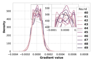
(a) Stage3 conv0 in Non-IID with hetero.

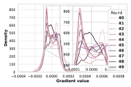
(b) Stage3 conv1 in Non-IID with hetero.

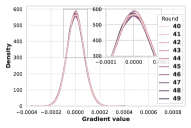
(c) Stage3 conv0 in IID with homo.

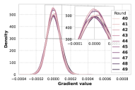
(d) Stage3 conv1 in IID with homo.

Figure 3: The gradient distributions from round 40 to 50 of Stage3 in Non-IID with heter and IID with homo.

Gradient Distributions. To dig out the latent relations between gradients and layer similarity, we delve deeper into the analysis of gradient distributions across different FL environments. More specifically, the comparison of Figure 2c and Figure 2d reveals that gradients from shallow layers (Stage3.conv0) exhibit greater similarity in distribution between Non-IID with hetero and IID with homo environments, in contrast to deep layers (Stage3.conv1 and Stage3.conv2). Additionally, as depicted in Figure 3c and Figure 3d, the distributions of gradients from a deep layer (Figure 3d) progressively approach the distribution of gradients from a shallow layer (Figure 3c) with each round, in contrast to Figure 3a and Figure 3b, where the distributions from deep layers (Figure 3b) are less smooth than those from shallow layers (Figure 3a) in Non-IID with hetero during rounds 40 to 50. Consequently, drawing from the aforementioned gradient analysis, we can enhance the quality of gradients from deep layers in Non-IID with hetero environments by leveraging gradients from shallow layers, i.e., cross-layer gradients as introduced in the subsequent section.

3 InCo Aggregation

We provide a concise overview of the three key components in InCo Aggregation at first. The first component is heterogeneous aggregation, which involves aggregating the model weights on a layer-by-layer basis instead of considering the entire model. The second component is the utilization of cross-layer gradients, where gradients from a shallow layer and a deep layer are combined to form the final gradients for updating the deep layer. However, directly using cross-layer gradients can lead to the issue of gradient divergence wang2020tackling ; zhao2018federated . To address this problem, the third component employs gradient normalization and introduces a convex optimization formulation. We elaborate on these three critical components of InCo Aggregation as follows.

3.1 Heterogeneous Aggregation

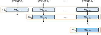
Figure 4: Heterogeneous aggregation for $n$ groups.

To facilitate model heterogeneity, we introduce an alternative aggregation, called heterogeneous aggregation, to accommodate most FL methods to the heterogeneous environment. Specifically, the weights of the same layer from different models would be averaged. For example, Figure 4 illustrates the heterogeneous aggregation for $n$ groups, $s_{1},...,s_{n}$. The clients in the same group share the same model architecture. $w_{l_{i},s_{j}}$ denotes the weights of layer $i$ in group $s_{j}$. We further use a superscript to denote that $w_{l_{i},s_{j}}^{k}$ belongs to the $k$-th client in group $s_{j}$. The group indexes are ordered by the size of the model architectures, i.e., the size of the client models in group $s_{1}$ is the smallest. As shown in the example in Figure 4, all groups share layer $1$, denoted by $w_{l_{1},s_{j}},j=1,...,n$. Then, layer $w_{l_{i}}$ only appears in group $\mathit{s}_{j}$ when $i\leq j$. Following the above definition, the heterogeneous aggregation for layer $w_{l_{i}}$ is expressed as $w_{l_{i}}=(\sum_{j=i}^{n}\sum_{k=1}^{|\mathit{s_{j}}|}w_{l_{i},\mathit{s}_{j}}^{k})/(\sum_{j=i}^{n}|\mathit{s_{j}}|)$, where $|\mathit{s_{j}}|$ denotes the number of clients in group $\mathit{s_{j}}$.

3.2 Cross-layer Gradients

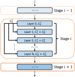
Figure 5: Cross-layer gradients for the server model in InCo.

Based on the findings of the case study, we observe that gradients from shallow layers contribute to increasing the similarity among layers from different clients. Therefore, we enhance the quality of gradients from deep layers by incorporating the utilization of cross-layer gradients. More specifically, when a server model updates the deep layers, we combine and refine the gradients from these layers with the gradients from the shallower layers to obtain appropriately updated gradients. Figure 5 provides a visual representation of how cross-layer gradients are employed. We focus on layers with matching shapes, indicating that they belong to the same stage of the entire model, such as the layer norm layer in Transformer lu2021pretrained . We assume that this stage has $N$ layers. The first layer satisfying the mentioned conditions is referred to as Layer 0, and its corresponding gradients at time step $t$ are $G_{0}^{t}$. For Layer $k$, where $k\in\{1,2,...,N\}$ within the same stage, the cross-layer gradients are given by $G_{k}^{t}+G_{0}^{t}$. Despite a large number of works on short-cut paths in neural networks, our method differs fundamentally in terms of the goals and the operations. We provide a thorough discussion in Appendix A.

3.3 Gradients Divergence Alleviation

However, the direct utilization of cross-layer gradients leads to an acute issue known as gradient and weight divergence wang2020tackling ; zhao2018federated , as depicted in Figure 6a. To counter this effect, our objective is to mitigate it through gradient normalization (Figure 6b) and the proposed convex optimization problem to restrict gradient directions, as illustrated in Figure 6c and described in Theorem 3.1.

Gradients Divergence Example. The gradient $g_{k}^{t}$ for layer $k$ at time $t$ guides the direction of the associated weights $w_{k}^{t}$ towards the client optimum point. When incorporating the shallow layer gradient $g_{0}^{t}$, represented by the right blue gradients in Figure 6a, the updated gradient becomes $g_{0}^{t}+g_{k}^{t}$, which moves the model a bit closer to the global optimum point than $g_{k}^{t}$ alone. Nevertheless, it still terminates at the client optimum point. To alleviate the negative impact of gradient divergence, we propose employing gradient normalization and formulating a convex optimization problem to restrict the directions of cross-layer gradients.

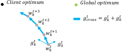
(a) Gradient divergence.

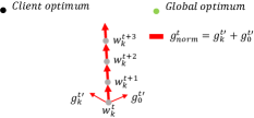
(b) Normalized gradients.

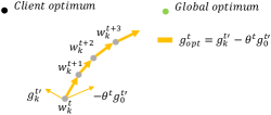
(c) Normalized and optimized.

Figure 6: A depiction of gradient divergence, as shown in Figure 6a, along with its solutions. Despite the normalization portrayed in Figure 6b, the impact of gradient divergence persists. To mitigate this issue, we propose a convex optimization problem that is restricting gradient directions, as demonstrated in Figure 6c and supported by Theorem 3.1.

Cross-layer Gradients Normalization. Figure 6b depicts the benefits of utilizing normalized gradients. The normalized cross-layer gradient ${g_{0}^{t}}^{\prime}+{g_{k}^{t}}^{\prime}$ directs the model closer to the global optimum than the original cross-layer gradient ${g_{0}^{t}}+{g_{k}^{t}}$. In particular, our normalization approach emphasizes the norm of gradients, i.e., ${g_{0}^{t}}^{\prime}=g_{0}^{t}/||g_{0}^{t}||$ and ${g_{k}^{t}}^{\prime}=g_{k}^{t}/||g_{k}^{t}||$. The normalized cross-layer gradient is computed as $({g_{0}^{t}}^{\prime}+{g_{k}^{t}}^{\prime})\times({||g_{0}^{t}||+||g_{k}^{t}||})/2$ in practice.

Convex Optimization. In addition to utilizing normalized gradients, incorporating novel projective gradients that leverage knowledge from both $g_{0}^{t}$ and $g_{k}^{t}$ serves to alleviate the detrimental impact of gradient divergence arising from the utilization of cross-layer gradients. Pursuing this line of thought, we introduce a constraint aimed at ensuring the optimization directions of gradients, outlined as $\langle g_{0}^{t},g_{k}^{t}\rangle\geq 0$, where $\langle\cdot,\cdot\rangle$ is the dot product. To establish a convex optimization problem incorporating this constraint, we denote the projected gradient as $g_{opt}$ and formulate the following primal convex optimization problem,

$$\min_{g_{opt}^{t}} ||g_{k}^{t}-g_{opt}^{t}||_{2}^{2},\ \ s.t.\ \langle g_{opt}^{t},g_{0}^{t}\rangle\geq 0,$$ (1)

where we preserve the optimization direction of $g_{0}^{t}$ in $g_{opt}^{t}$ while minimizing the distance between $g_{opt}^{t}$ and $g_{k}^{t}$. We prioritize the proximity of $g_{opt}^{t}$ to $g_{k}^{t}$ over $g_{0}^{t}$ since $g_{k}^{t}$ represents the true gradients of layer $k$. By solving this problem through Lagrange dual problem bot2009duality , we derive the following outcomes,

Theorem 3.1.

(Divergence alleviation). If gradients are vectors, for the layers that require cross-layer gradients, their updated gradients can be expressed as,

$$g_{opt}^{t}=\begin{cases}g_{k}^{t},&\text{if }\beta\geq 0\\ g_{k}^{t}-\theta^{t}g_{0}^{t},&\text{if }\beta<0,\end{cases}$$ (2)

where $\theta^{t}=\frac{\beta}{\alpha}$, $\alpha=(g_{0}^{t})^{T}g_{0}^{t}$ and $\beta=(g_{0}^{t})^{T}g_{k}^{t}$.

Remark 3.2.

This theorem can be extended to the matrix form.

We provide proof for Theorem 3.1 and demonstrate how matrix gradients are incorporated into the problem in Appendix B. Our analytic solution in Equation 2 automatically determines the optimal settings for parameter $\theta^{t}$, eliminating the need for cumbersome manual adjustments. In our practical implementation, we consistently update the server model using the expression $g_{k}^{t}-\theta^{t}g_{0}^{t}$, irrespective of whether $\beta\leq 0$ or $\beta<0$. This procedure is illustrated in Algorithm 1 in Appendix F.

4 Convergence Analysis

In this section, we demonstrate the convergence of cross-layer gradients and propose the convergence rate in non-convex scenarios. To simplify the notations, we adopt $L_{i}$ to be the local objective. At first, we show the following assumptions frequently used in the convergence analysis for FL tan2022fedproto ; li2018federated ; karimireddy2020scaffold .

Assumption 4.1.

(Lipschitz Smooth). Each objective function $L_{i}$ is $L$-Lipschitz smooth and satisfies that $||\nabla L_{i}(x)-\nabla L_{i}(y)||\leq L||x-y||,\forall(x,y)\in D_{i},i\in{1,...,K}$.

Assumption 4.2.

(Unbiased Gradient and Bounded Variance). At each client, the stochastic gradient is an unbiased estimation of the local gradient, with $\mathbb{E}[g_{i}(x)])=\nabla L_{i}(x)$, and its variance is bounded by $\sigma^{2}$, meaning that $\mathbb{E}[||g_{i}(x)-\nabla L_{i}(x)||^{2}]\leq\sigma^{2},\forall i\in{1,...,K}$, where $\sigma^{2}\geq 0.$

Assumption 4.3.

(Bounded Expectation of Stochastic Gradients). The expectation of the norm of the stochastic gradient at each client is bounded by $\rho$, meaning that $\mathbb{E}[||g_{i}(x)||]\leq\rho,\forall i\in{1,...,K}$.

Assumption 4.4.

(Bounded Covariance of Stochastic Gradients). The covariance of the stochastic gradients is bounded by $\Gamma$, meaning that $Cov(g_{i,l_{k}},g_{i,l_{j}})\leq\Gamma,\forall i\in{1,...,K}$, where $l_{k},l_{j}$ are the layers belonging to a model at client $i$.

Following these assumptions, we present the proof of non-convex convergence concerning the utilization of cross-layer gradients in Federated Learning (FL). We outline our three principal theorems as follows.

Theorem 4.5.

(Per round drift). Supposed Assumption 4.1 to Assumption 4.4 are satisfied, the loss function of an arbitrary client at round $t+1$ is bounded by,

$$\mathbb{E}[L_{t+1,0}]\leq\mathbb{E}[L_{t,0}]-(\eta-\frac{L\eta^{2}}{2})\sum_{e=0}^{E-1}||\nabla L_{t,e}||^{2}+\frac{LE\eta^{2}}{2}\sigma^{2}+2\eta(\Gamma+\rho^{2})+L\eta^{2}(2\rho^{2}+\sigma^{2}+\Gamma).$$ (3)

The Theorem 3 demonstrates the bound of the local objective function after every communication round. Non-convex convergence can be guaranteed by the appropriate $\eta$.

Theorem 4.6.

(Non-convex convergence). The loss function L is monotonously decreased with the increasing communication round when,

$$\eta<\frac{2\sum_{e=0}^{E-1}||\nabla L_{t,e}||^{2}-4(\Gamma+\rho^{2})}{L(\sum_{e=0}^{E-1}||\nabla L_{t,e}||^{2}+E\rho^{2}+2(2\rho^{2}+\sigma^{2}+\Gamma)}.$$ (4)

Moreover, after we prove the non-convex convergence for the cross-layer gradients, the non-convex convergence rate is described as follows.

Theorem 4.7.

(Non-convex convergence rate). Supposed Assumption 4.1 to Assumption 4.4 are satisfied and $\kappa=L_{0}-L^{*}$, for an arbitrary client, given any $\epsilon>0$, after

$$T=\frac{2\kappa}{E\eta((2-L\eta)\epsilon-3L\eta\sigma^{2}-2(2+L\eta)\Gamma-4(1+L\eta)\rho^{2})}$$ (5)

communication rounds, we have

$$\frac{1}{TE}\sum_{t=0}^{T-1}\sum_{e=0}^{E-1}\mathbb{E}[||\nabla L_{t,e}||^{2}]\leq\epsilon,\ \textit{if}\ \ \ \eta<\frac{2\epsilon-4(\Gamma+\rho^{2})}{L(\epsilon+E\rho^{2}+2(2\rho^{2}+\sigma^{2}+\Gamma))}.$$ (6)

Following these theorems, the convergence of cross-layer gradients is guaranteed. The proof is presented in Appendix C.

5 Experiments

In this section, we conduct comprehensive experiments aimed at demonstrating three fundamental aspects: (1) the efficacy of InCo Aggregation and its extensions for various FL methods (Section 5.2), (2) the robustness analysis and ablation study of InCo Aggregation (Section 5.3), (3) in-depth analyses of the underlying principles behind InCo Aggregation (Section 5.4). Our codes will be released on Github. More experimental details and results can be found in Appendix F.

5.1 Experiment Setup

Dataset and Data Distribution. We conduct experiments on Fashion-MNIST xiao2017/online , SVHN netzer2011reading , CIFAR-10 krizhevsky2009learning and CINIC-10 darlow2018cinic under non-iid settings. We evaluate the algorithms under two Dirichlet distributions with $\alpha=0.5$ and $\alpha=1.0$ for all datasets.

Baselines. To demonstrate the effectiveness of InCo Aggregation, we use five prominent baselines in model-homogeneous FL: FedAvg mcmahan2017communication , FedProx li2018federated , FedNova wang2020tackling , Scaffold karimireddy2020scaffold , and MOON li2021model for ResNets and ViTs. We employ the training methodology outlined in lin2020ensemble to conduct the training procedures for these baselines within model heterogeneous environments. By incorporating these methods with InCo Aggregation, we obtain InCoAvg, InCoProx, InCoNova, InCoScaffold, and InCoMOON. We take the average accuracy of three different random seeds. Our implementations of the baselines are referred to li2022federated .

Federated Settings. In heterogeneous FL, we consider two distinctive architectures, ResNets and ViTs, each comprising five different models. The ResNet models are ResNet10, ResNet14, ResNet18, ResNet22, and ResNet26 from the PyTorch source codes. For the pretrained ViT models, we employ ViT-S/8, ViT-S/9, ViT-S/10, ViT-S/11, and ViT-S/12 from the PyTorch Image Models (timm). Our experimental setup involves 100 clients, with a sample ratio of 0.1. To accommodate the five different architectures, all clients are categorized into five distinct groups.

Table 2: Test accuracy of 100 clients and sample ratio 0.1. We shade in gray the methods that are combined with our proposed method, InCo Aggregation. We bold the best results and denote the improvements compared to the original methods in red.

Base	Methods	Fashion-MNIST		SVHN		CIFAR10		CINIC10
		$\alpha=0.5$	$\alpha=1.0$	$\alpha=0.5$	$\alpha=1.0$	$\alpha=0.5$	$\alpha=1.0$	$\alpha=0.5$	$\alpha=1.0$
ResNet	FedAvg	86.7$\pm$1.0	87.7$\pm$0.6	74.8$\pm$3.2	81.6$\pm$2.5	52.3$\pm$3.4	61.3$\pm$3.2	43.1$\pm$2.7	49.2$\pm$3.1
	FedProx	75.1$\pm$1.8	76.6$\pm$1.5	32.0$\pm$2.8	43.7$\pm$2.9	19.2$\pm$2.2	23.4$\pm$2.4	17.4$\pm$1.7	19.8$\pm$1.4
	Scaffold	87.9$\pm$0.5	88.0$\pm$0.3	76.3$\pm$3.4	82.4$\pm$3.1	54.3$\pm$3.6	61.8$\pm$3.0	43.5$\pm$2.4	49.4$\pm$3.1
	FedNova	12.7$\pm$0.2	15.6$\pm$0.2	13.4$\pm$ 0.4	15.3$\pm$0.3	10.4$\pm$0.3	14.3$\pm$0.2	12.0$\pm$0.3	14.0$\pm$0.2
	MOON	87.7$\pm$0.4	87.5$\pm$0.3	72.8$\pm$4.3	81.2$\pm$3.2	47.2$\pm$2.7	58.8$\pm$2.6	40.8$\pm$2.1	49.2$\pm$ 1.9
	InCoAvg	90.2($\uparrow$3.5)	88.4($\uparrow$0.7)	87.6($\uparrow$12.8)	89.0($\uparrow$7.4)	67.8($\uparrow$15.5)	70.7($\uparrow$9.4)	53.0($\uparrow$9.9)	57.5($\uparrow$8.3)
	InCoProx	88.8($\uparrow$13.7)	86.4($\uparrow$9.8)	89.0($\uparrow$57.0)	90.8($\uparrow$47.1)	74.5($\uparrow$55.3)	76.8($\uparrow$53.4)	59.1($\uparrow$41.7)	62.5($\uparrow$42.7)
	InCoScaffold	88.3($\uparrow$0.4)	90.1($\uparrow$2.1)	85.4($\uparrow$9.1)	87.8($\uparrow$5.4)	67.3($\uparrow$13.0)	73.8($\uparrow$12.0)	53.5($\uparrow$10.0)	61.7($\uparrow$12.3)
	InCoNova	86.6($\uparrow$73.9)	87.4($\uparrow$71.8)	86.4($\uparrow$73.0)	88.4($\uparrow$73.1)	62.8($\uparrow$52.4)	69.7($\uparrow$55.4)	48.0($\uparrow$36.0)	54.1($\uparrow$40.1)
	InCoMOON	89.1($\uparrow$1.4)	89.5($\uparrow$2.0)	85.6($\uparrow$12.8)	89.3($\uparrow$8.1)	68.2($\uparrow$21.0)	71.8($\uparrow$13.0)	54.3($\uparrow$13.5)	57.6($\uparrow$8.4)
ViT	FedAvg	92.0$\pm$0.7	91.9$\pm$0.5	92.4$\pm$0.9	93.9$\pm$0.8	93.7$\pm$1.0	94.2$\pm$0.8	83.8$\pm$1.4	85.1$\pm$0.9
	FedProx	89.8$\pm$0.5	89.7$\pm$0.5	71.4$\pm$3.8	81.1$\pm$2.9	82.6$\pm$3.3	84.7$\pm$2.3	67.8$\pm$2.8	71.3$\pm$3.0
	Scaffold	92.0$\pm$0.4	92.0$\pm$0.5	92.2$\pm$0.8	93.8$\pm$0.6	93.5$\pm$0.7	94.5$\pm$0.5	83.3$\pm$1.6	85.5$\pm$1.2
	FedNova	70.3$\pm$0.5	76.7$\pm$0.4	27.4$\pm$0.4	49.8$\pm$0.5	30.7$\pm$0.3	54.4$\pm$0.5	31.6$\pm$1.5	50.7$\pm$1.3
	MOON	92.1$\pm$0.3	92.1$\pm$0.2	92.5$\pm$1.2	93.9$\pm$0.9	93.6$\pm$0.8	94.6$\pm$0.3	84.3$\pm$1.6	85.3$\pm$1.2
	InCoAvg	93.0($\uparrow$1.0)	93.1($\uparrow$1.2)	94.2($\uparrow$1.8)	95.0($\uparrow$1.1)	94.6($\uparrow$0.9)	95.0($\uparrow$0.8)	85.9($\uparrow$2.1)	86.8($\uparrow$1.7)
	InCoProx	92.6($\uparrow$2.8)	92.5($\uparrow$2.8)	93.9($\uparrow$22.5)	94.4($\uparrow$13.3)	94.0($\uparrow$11.4)	94.8($\uparrow$10.1)	85.1 ($\uparrow$17.3)	86.0($\uparrow$14.7)
	InCoScaffold	92.9($\uparrow$0.9)	93.0($\uparrow$1.0)	94.0($\uparrow$1.8)	94.8($\uparrow$1.0)	94.6($\uparrow$1.1)	95.0($\uparrow$0.5)	85.7($\uparrow$2.4)	86.5($\uparrow$1.0)
	InCoNova	93.1($\uparrow$22.8)	93.6($\uparrow$16.9)	94.7($\uparrow$67.3)	95.6($\uparrow$45.8)	94.8($\uparrow$64.1)	95.7($\uparrow$41.3)	86.2($\uparrow$54.6)	88.2($\uparrow$37.5)
	InCoMOON	92.8($\uparrow$0.7)	93.0($\uparrow$0.9)	94.7($\uparrow$2.2)	95.1($\uparrow$1.2)	94.2($\uparrow$0.6)	95.1 ($\uparrow$0.5)	86.0($\uparrow$1.7)	86.8($\uparrow$1.5)

5.2 Extending Homogeneity to Heterogeneity.

Table 2 presents the test accuracy of 100 clients with a sample ratio of 0.1. We state the improvements of each baseline in the table. The error bars of InCo Aggregation methods are shown in Appendix F.

InCo Aggregation Improves All Baselines. Table 2 provides compelling evidence for the efficacy of InCo Aggregation in enhancing the performance of all baselines. Particularly noteworthy is the substantial improvement achieved by FedNova, which previously struggled to converge but now achieves comparable performance through the adoption of InCo Aggregation. Furthermore, baselines such as FedProx demonstrate significant accuracy profits (around 10%) when leveraging InCo Aggregation on the server side. This pattern of remarkable improvement extends to other baselines as well. Moreover, InCo Aggregation gains more improvements in the CIFAR-10 and CINIC-10 compared to Fashion-MNIST, which suggests that InCo Aggregation exhibits greater effectiveness in more challenging datasets. These results are inspiring, as InCo Aggregation achieves substantial improvements without incurring any additional communication overheads compared to the original baselines.

5.3 Robustness Analysis and Ablation Study.

We delve into the robustness analysis of InCo Aggregation, examining two key aspects: (1) the impact of varying batch sizes, and (2) the effect of noise perturbations on gradients during transmission. Additionally, we perform an ablation study to assess the contributions of the key components in InCo Aggregation. Throughout this subsection, we use InCoAvg as a representative measure of the performance achieved by InCo Aggregation, with FedAvg serving as the baseline. For a comprehensive exploration across different baselines, we provide detailed experiments in Appendix F.

Effect of Batch Size and Noise Perturbation. Figure 7 presents the outcomes of the robustness analysis for InCo Aggregation. Notably, when compared to FedAvg as depicted in Figure 7a and Figure 7b, our method exhibits significant improvements while maintaining comparable performance across all settings. Remarkably, even the best results achieved by FedAvg under any condition are surpassed by the worst results obtained by InCoAvg. Furthermore, as illustrated in Figure 7c and Figure 7d, we explore the impact of different noise perturbations by simulating noise with standard deviations following the gradients. The results demonstrate substantial performance gains achieved by InCo Aggregation, affirming its robustness in the face of noise perturbations, as well as the protection of client privacy because of the incorporation of noise in the transmitted gradients.

Ablation Study. Our ablation study includes the following methods: (i) InCoAvg w/o Normalization (HeteroAvg with cross-layer gradients and optimization), (ii) InCoAvg w/o Optimization (HeteroAvg with normalized cross-layer gradients), (iii) InCoAvg w/o Normalization and Optimization (HeteroAvg with cross-layer gradients), and (iv) HeteroAvg (FedAvg with heterogeneous aggregation). The ablation study of InCo Aggregation is depicted in Figure 8. Firstly, the inferior performances of InCoAvg w/o Normalization highlight the critical role of gradient normalization in achieving effective InCo Aggregation. Furthermore, directly utilizing cross-layer gradients (InCoAvg w/o N & O) is shown to be worse than not using them at all (HeteroAvg) in certain cases, underscoring the importance of both gradient normalization and optimization. Finally, the observed improvement between InCoAvg and InCoAvg w/o Optimization demonstrates the effectiveness of Theorem 3.1.

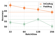
(a) Different batch sizes in CIFAR-10.

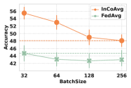
(b) Different batch sizes in CINIC-10.

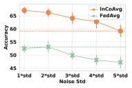
(c) Different noise perturbations in CIFAR-10.

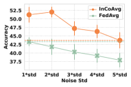
(d) Different noise perturbations in CINIC-10.

Figure 7: Robustness analysis for InCo Aggregation.

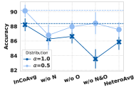
(a) Fashion-MNIST.

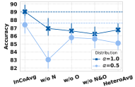
(b) SVHN.

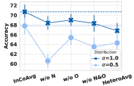
(c) CIFAR-10.

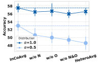
(d) CINIC-10.

Figure 8: Ablation studies for InCo Aggregation. These studies are conducted on four datasets with two different data distributions. The federated settings are the same as Table 2.

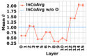
(a) $\theta$ in all layers.

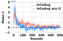
(b) $\beta$ in Layer 11.

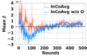
(c) $\beta$ in Layer 13.

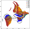
(d) FedAvg.

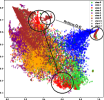
(e) HeteroAvg.

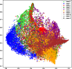
(f) InCoAvg.

Figure 9: Important coefficients of Theorem 3.1 and t-SNE visualization of features. (a): $\theta$ in all layers. (b) $\beta$ in Layer 11. (c) $\beta$ in Layer 13. (d) to (e): t-SNE visualization of features learned by different methods on CIFAR-10. We select six classes and three clients (one ResNet22 and two ResNet26) to simplify the notations in t-SNE figures.

5.4 The Reasons for the Improvements

We undertake a comprehensive analysis to gain deeper insights into the mechanisms underlying the efficacy of InCo Aggregation. Our analysis focuses on three key aspects: (1) The investigation of important coefficients $\theta$ and $\beta$ in Theorem 3.1. (2) An examination of the feature spaces generated by different methods. (3) The evaluation of CKA similarity across various layers.

Analysis for $\theta$. In our experiments, we set $\theta=1$ for InCoAvg w/o Optimization, the blue dash line in Figure 9a. However, under Theorem 3.1, we observe that the value of $\theta$ varies for different layers, indicating the effectiveness of the theorem in automatically determining the appropriate $\theta$ values. Notably, adjacent layers within the same neural network basic block, such as BasicBlock and Bottleneck in PyTorch source codes, exhibit similar $\theta$ values, reflecting their shared shallow layer gradients and resulting in similar $\theta$ values.

Analysis for $\beta$. $\beta>0$ denotes the same direction between shallow layer gradients and the current layer gradients. Through the analysis of Figure 9b and Figure 9c, $\beta$ decreases with an increase in the number of communication rounds, reflecting the diminishing gradients during the training process. Furthermore, in the case of InCoAvg, Layer 11 demonstrates that 83.8% of $\beta$ values are greater than 0, while Layer 13 exhibits 74.4% of $\beta$ values greater than 0. In contrast, InCoAvg without Optimization achieves only 53.5% and 50.2% of $\beta$ values greater than 0, as indicated in Table 3. These findings provide empirical evidence supporting the efficacy of Theorem 3.1 in heterogeneous FL.

Table 3: The Percentage of $\beta>0$

Methods	Percentage of $\beta>0$
	Layer 11	Layer 13
InCoAvg	83.8	74.4
InCoAvg w/o O	53.5	50.2

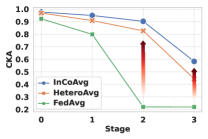
(a) CIFAR10 with $\alpha=0.5$.

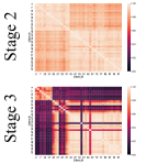
(b) InCoAvg.

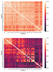
(c) HeteroAvg.

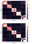
(d) FedAvg.

CID InCoAvg HeteroAvg 0 54.4 54.8 20 70.7 67.8 40 75.3 72.6 60 73.3 69.9 80 72.0 68.5

(e) Client Accuracy.

Figure 10: CKA layer similarity, Heatmaps and accuracy of different clients. (a): The layer similarity of different methods. (b) to (d): Heatmaps for different methods in stage 2 and stage 3. (e): Accuracy of each client group. (0: ResNet10, 20: ResNet14, 40: ResNet18, 60: ResNet22, 80: ResNet26)

t-SNE Visualizations for Different Methods. Figure 9d to Figure 9f demonstrate the t-SNE visualization van2008visualizing of features learned by different methods on the CIFAR-10 dataset. It is obvious that model drift occurs in FedAvg, as shown in Figure 9d, which means that the features from the same class are separated by clients with different architectures (client 0, 1, and 2), indicating a lack of feature extraction and learning across clients with different architectures. Figure 9e shows that model drift is mitigated in HeteroAvg, but feature drift is observed, as features from the same class scatter into different clusters. In contrast, InCoAvg addresses both model drift and feature drift concurrently, as demonstrated in Figure 9f, which is no evidence of similar phenomena in the feature space, highlighting the effectiveness of InCo Aggregation.

Analysis for CKA Layer Similarity. Figure 10a reveals that InCoAvg exhibits a significantly higher CKA layer similarity compared to FedAvg, accompanied by improved accuracy. This finding provides evidence that InCo Aggregation enhances layer similarity to achieve superior performance. Heatmaps from stage 2 to stage 3 for various methods are presented in Figure 10b to Figure 10d. Consistent with the t-SNE visualization, FedAvg’s heatmaps exhibit block-wise patterns due to its inability to extract features from diverse model architectures. In stage 2, a substantial improvement in CKA similarity is observed for InCoAvg compared to HeteroAvg and FedAvg. Notably, the smallest models in InCoAvg (top left corner) exhibit lower similarity (more black) with other clients compared to HeteroAvg in stage 3, while the larger models in InCoAvg demonstrate much higher similarity than HeteroAvg. This discrepancy arises because the accuracy of the smallest models in InCoAvg is similar to that of HeteroAvg, but the performance of larger models in InCoAvg surpasses that of HeteroAvg, as indicated in Figure 10e. Consequently, a larger similarity gap emerges between the smallest models and the other models. Addressing the performance of the smallest models in InCo Aggregation represents our future research direction.

6 Conclusions

In this paper, we present a case study that highlights the positive correlation between client performance and layer similarity in FL. Motivated by this observation, we propose a novel FL training scheme called InCo Aggregation, which aims to enhance the capabilities of model-homogeneous FL methods in heterogeneous FL settings. Our approach leverages normalized cross-layer gradients to promote similarity among deep layers across different clients. Additionally, we introduce a convex optimization formulation to address the challenge of gradient divergence. Through extensive experimental evaluations, we demonstrate the effectiveness of InCo Aggregation in improving heterogeneous FL performance. Furthermore, our detailed analysis of InCo Aggregation sheds light on the potential of leveraging internal cross-layer gradients as a promising direction to facilitate and improve the performance of heterogeneous FL.

Limitations and Future works. The objective of this study is to expand the capabilities of model-homogeneous methods to effectively handle model-heterogeneous FL environments. However, the analysis of layer similarity reveals that the smallest models do not derive substantial benefits from InCo Aggregation, implying the limited extensions for these smallest models. Exploring methods to enhance the performance of the smallest models warrants further investigation. Furthermore, our research mainly focuses on image classification tasks, specifically CNN models (ResNets) and Transformers (ViTs). However, it is imperative to validate our conclusions in the context of language tasks and other architectural models such as LSTM. hochreiter1997long . We believe that it is worth extending this work to encompass a wider range of tasks and diverse model architectures that hold great value and potential for future research.

Appendix A Comparisons with Residual Connections

Remarks on self-mixture approaches in neural networks. The goal of residual connections is to avoid exploding and vanishing gradients to facilitate the training of a single model he2016identity , while cross-layer gradients aim to increase the layer similarities across a group of models that are jointly optimized in federated learning. Specifically, residual connections modify forward passes by adding the shallow-layer outputs to those of the deep layers. In contrast, cross-layer gradients operate on the gradients calculated by back-propagation. We present the distinct gradient outcomes of the two methods in the following.

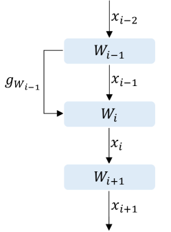
(a) Cross-layer gradients

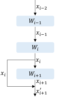
(b) Residual connections

Figure 11: Comparison of cross-layer gradients and residual connections

Consider three consecutive layers of a feedforward neural network indexed by $i-1,i,i+1$. With a slight abuse of symbols, we use $f(\,\cdot\,;W_{k})$ to denote the calculation in the $k$-th layer. Given the input $\mathbf{x_{i-2}}$ to layer $i-1$, the output from the previous layer becomes the input to the next layer, thus generating $\mathbf{x_{i-1}},\mathbf{x_{i}},\mathbf{x_{i+1}}$ sequentially.

$$\mathbf{x_{i-1}} =f(\mathbf{x_{i-2}};W_{i-1})$$ (7)

$$\mathbf{x_{i}} =f(\mathbf{x_{i-1}};W_{i})$$

$$\mathbf{x_{i+1}} =f(\mathbf{x_{i}};W_{i+1})$$

In the case of residual connections, there is an additional operation that directs $\mathbf{x_{i}}$ to $\mathbf{x_{i+1}}$, formulated as $\mathbf{x_{i+1}^{\prime}}=\mathbf{x_{i+1}}+\mathbf{x_{i}}$. The gradient of $W_{i}$ is

$$g_{W_{i}} =\frac{\partial loss}{\partial W_{i}}$$ (8)

$$=\frac{\partial loss}{\partial\mathbf{x_{i+1}^{\prime}}}\cdot\frac{\partial\mathbf{x_{i+1}^{\prime}}}{\partial\mathbf{x_{i}}}\cdot\frac{\partial\mathbf{x_{i}}}{\partial W_{i}}$$

$$=\frac{\partial loss}{\partial(\mathbf{x_{i+1}}+\mathbf{x_{i}})}\cdot\left(\frac{\partial\mathbf{x_{i+1}}}{\partial\mathbf{x_{i}}}+\mathbb{1}\right)\cdot\frac{\partial\mathbf{x_{i}}}{\partial W_{i}}$$

$$=\frac{\partial loss}{\partial(\mathbf{x_{i+1}}+\mathbf{x_{i}})}\cdot\left(\frac{\partial\mathbf{x_{i+1}}}{\partial W_{i}}+\frac{\partial\mathbf{x_{i}}}{\partial W_{i}}\right)$$

In the case of cross-layer gradients, the gradient of $W_{i}$ is

$$g_{W_{i}} =\frac{\partial loss}{\partial W_{i}}+\frac{\partial loss}{\partial W_{i-1}}$$ (9)

$$=\frac{\partial loss}{\partial\mathbf{x}_{i+1}}\cdot\left(\frac{\partial\mathbf{x_{i+1}}}{\partial W_{i}}+\frac{\partial\mathbf{x_{i+1}}}{\partial W_{i-1}}\right)$$

We note that both residual connections and cross-layer gradients are subject to certain constraints. Residual connections requires identical shapes for the layer outputs, while cross-layer gradients operate on the layer weights with the same shape.

Appendix B Proof of Theorem 3.1

This section demonstrates the details of the proof of Theorem 3.1. We will present the proof of Theorem 3.1 in the vector form and the matrix form.

B.1 Vector Form

We state the convex optimization problem Theorem 1 in the vector form in the following,

$$\min_{g_{opt}} ||g_{k}-g_{opt}||_{2}^{2},$$ (10)

$$s.t. \langle g_{opt},g_{0}\rangle\geq 0.$$

Because the superscript $t$ would not influence the proof of the theorem, we simplify the notation $g^{t}$ to $g$. We use Equation 10 instead of Equation 1 to complete this proof. The Lagrangian of Equation 10 is shown as,

$$L(g_{opt},\lambda)= (g_{k}-g_{opt})^{T}(g_{k}-g_{opt})-\lambda g_{opt}^{T}g_{0}$$ (11)

$$= g_{k}^{T}g_{k}-g_{opt}^{T}g_{k}-g_{k}^{T}g_{opt}+g_{opt}^{T}g_{opt}-\lambda g_{opt}^{T}g_{0}$$

$$= g_{k}^{T}g_{k}-2g_{opt}^{T}g_{k}+g_{opt}^{T}g_{opt}-\lambda g_{opt}^{T}g_{0}.$$

Let $\frac{\partial L(g_{opt},\lambda)}{\partial g_{opt}}=0$, we have

$$g_{opt}=g_{k}+\lambda g_{0}/2,$$ (12)

which is the optimum point for the primal problem Equation 10. To get the Lagrange dual function $L(\lambda)=\inf_{g_{opt}}L(g_{opt},\lambda)$, we substitute $g_{opt}$ by $g_{k}+\lambda g_{0}/2$ in $L(g_{opt},\lambda)$. We have

$$L(\lambda)= g_{k}^{T}g_{k}-2(g_{k}+\frac{\lambda g_{0}}{2})^{T}g_{k}+(g_{k}+\frac{\lambda g_{0}}{2})^{T}(g_{k}+\frac{\lambda g_{0}}{2})-\lambda(g_{k}+\frac{\lambda g_{0}}{2})^{T}g_{0}$$ (13)

$$= g_{k}^{T}g_{k}-2g_{k}^{T}g_{k}-\lambda g_{0}^{T}g_{k}+g_{k}^{T}g_{k}+\frac{\lambda g_{0}^{T}g_{k}}{2}+\frac{\lambda g_{k}^{T}g_{0}}{2}+\frac{\lambda^{2}g_{0}^{T}g_{0}}{4}-\lambda g_{k}^{T}g_{0}-\frac{\lambda^{2}g_{0}^{T}g_{0}}{2}$$

$$= g_{k}^{T}g_{k}-2g_{k}^{T}g_{k}+g_{k}^{T}g_{k}-\lambda g_{0}^{T}g_{k}+\lambda g_{0}^{T}g_{k}+\frac{\lambda^{2}g_{0}^{T}g_{0}}{4}-\frac{\lambda^{2}g_{0}^{T}g_{0}}{2}-\lambda g_{k}^{T}g_{0}$$

$$= -\frac{g_{0}^{T}g_{0}}{4}\lambda^{2}-g_{k}^{T}g_{0}\lambda.$$

Thus, the Lagrange dual problem is described as follows,

$$\max_{\lambda} L(\lambda)=-\frac{g_{0}^{T}g_{0}}{4}\lambda^{2}-g_{k}^{T}g_{0}\lambda,$$ (14)

$$s.t. \lambda\geq 0.$$

$L(\lambda)$ is a quadratic function. Because $g_{0}^{T}g_{0}\geq 0$, the maximum of $L(\lambda)$ is at the point $\lambda=-\frac{2b}{a}$ where $a=g_{0}^{T}g_{0}$ and $b=g_{k}^{T}g_{0}$ if we do not consider the constraint. It is clear that this convex optimization problem holds strong duality because it satisfies Slater’s constraint qualificationboyd2004convex , which indicates that the optimum point of the dual problem Equation 14 is also the optimum point for the primal problem Equation 10. We substitute $\lambda$ by $-\frac{2b}{a}$ in Equation 12, and we have

$$g_{opt}=\begin{cases}g_{k},&\text{if }b\geq 0,\\ g_{k}-\theta^{t}g_{0},&\text{if }b<0,\end{cases}$$ (15)

where $\theta^{t}=\frac{b}{a}$, $a=(g_{0})^{T}g_{0}$ and $b=g_{k}^{T}g_{0}$. We add the superscript $t$ to all gradients, and we finish the proof of Theorem 3.1.

B.2 Matrix Form

The proof of the matrix form is similar to Appendix B.1. We update Equation 10 to the matrix form as follows,

$$\min_{G_{opt}} ||G_{k}-G_{opt}||_{F}^{2},$$ (16)

$$s.t. \langle G_{opt},G_{0}\rangle\geq 0.$$

Similar to Equation 11, the Lagragian of Equation 16 is,

$$L(G_{opt},\lambda)=tr(G_{k}^{T}G_{k})-tr(G_{opt}^{T}G_{k})-tr(G_{k}^{T}G_{opt})+tr(G_{opt}^{T}G_{opt})-\lambda tr(G_{opt}^{T}G_{0}),$$ (17)

where $tr(A)$ means the trace of the matrix $A$. We can obtain the optimum point for Equation 16 according to $\frac{\partial L(G_{opt},\lambda)}{\partial G_{opt}}=0$. We have

$$G_{opt}=G_{k}+\lambda G_{0}/2.$$ (18)

Similar to the analysis in Appendix B.1 and Equation 13, we get the Lagrange dual problem as follows,

$$\max_{\lambda} L(\lambda)=-\frac{tr(G_{0}^{T}G_{0})}{4}\lambda^{2}-tr(G_{k}^{T}G_{0})\lambda,$$ (19)

$$s.t. \lambda\geq 0,$$

where $tr(G_{0}^{T}G_{0})\geq 0$. Following the same analysis in Appendix B.1, we have

$$G_{opt}=\begin{cases}G_{k},&\text{if }b\geq 0,\\ G_{k}-\theta^{t}G_{0},&\text{if }b<0,\end{cases}$$ (20)

where $\theta^{t}=\frac{b}{a}$, $a=tr(G_{0}^{T}G_{0})$ and $b=tr(G_{k}^{T}G_{0})$. At last we have finish the proof of the matrix form of Theorem 3.1.

Appendix C Proof of Convergence Analysis

We show the details of convergence analysis for cross-layer gradients. $W^{l_{i}}_{t,e}$ are the weights from the layers which need cross-layer gradients at round $t$ of the local step $e$. To simplify the notations, we use $W_{t,e}$ instead of $W^{l_{i}}_{t,e}$.

Lemma C.1.

(Per Round Progress.) Suppose our functions satisfy Assumption 4.1 and Assumption 4.2. The expectation of a loss function of any arbitrary clients at communication round $t$ after $E$ local steps is bounded as,

$$\mathbb{E}[L_{t,E-1}]\leq\mathbb{E}[L_{t,0}]-(\eta-\frac{L\eta^{2}}{2})\sum_{e=0}^{E-1}||\nabla L_{t,e}||^{2}+\frac{LE\eta^{2}}{2}\sigma^{2}.$$ (21)

Proof.

Considering an arbitrary client, we omit the client index $i$ in this lemma. Let $W_{t,e+1}=W_{t,e}-\eta g_{t,e}$, we have

$$L_{t,e+1} \leq L_{t,e}+\langle\nabla L_{t,e},W_{t,e+1}-W_{t,e}\rangle+\frac{L}{2}||W_{t,e+1}-W_{t,e}||^{2}$$ (22)

$$\leq L_{t,e}-\eta\langle\nabla L_{t,e},g_{t,e}\rangle+\frac{L}{2}||\eta g_{t,e}||^{2},$$

where Equation 22 follows Assumption 4.1. We take expectation on both sides of Equation 22, then

$$\mathbb{E}[L_{t,e+1}] \leq\mathbb{E}[L_{t,e}]-\eta\mathbb{E}[\langle\nabla L_{t,e},g_{t,e}\rangle]+\frac{L}{2}\mathbb{E}[||\eta g_{t,e}||^{2}]$$ (23)

$$=\mathbb{E}[L_{t,e}]-\eta||\nabla L_{t,e}||^{2}+\frac{L\eta^{2}}{2}\mathbb{E}[||g_{t,e}||^{2}]$$

$$\overset{(a)}{=}\mathbb{E}[L_{t,e}]-\eta||\nabla L_{t,e}||^{2}+\frac{L\eta^{2}}{2}(\mathbb{E}[||g_{t,e}||]^{2}+Var(||g_{t,e}||))$$

$$=\mathbb{E}[L_{t,e}]-\eta||\nabla L_{t,e}||^{2}+\frac{L\eta^{2}}{2}(||\nabla L_{t,e}||^{2}+Var(||g_{t,e}||))$$

$$\overset{(b)}{\leq}\mathbb{E}[L_{t,e}]-(\eta-\frac{L\eta^{2}}{2})||\nabla L_{t,e}||^{2}+\frac{L\eta^{2}}{2}\sigma^{2},$$

where (a) follows $Var(X)=\mathbb{E}[X^{2}]-\mathbb{E}^{2}[X]$, and (b) is Assumption 4.2. Telescoping local step 0 to $E-1$, we have

$$\mathbb{E}[L_{t,E-1}]\leq\mathbb{E}[L_{t,0}]-(\eta-\frac{L\eta^{2}}{2})\sum_{e=0}^{E-1}||\nabla L_{t,e}||^{2}+\frac{LE\eta^{2}}{2}\sigma^{2},$$ (24)

then we finish the proof of Lemma C.1.

Lemma C.2.

(Bound Client Dirft.) Suppose our functions satisfy Assumption 4.2, Assumption 4.3 and Assumption 4.4. After each aggregation, the updates, $\Delta W$, for the layers need cross-layer gradients have bounded drift:

$$\mathbb{E}[||\Delta W||^{2}]\leq 2\eta^{2}(2\rho^{2}+\sigma^{2}+\Gamma).$$ (25)

Proof.

We have $W_{t+1,0}-W_{t,E-1}=\Delta W=\eta(g_{l_{0}}+g_{l_{i}}),\forall l_{i}$ need cross-layer gradients. Because all gradients are in the same aggregation round, we omit the time subscript in this proof process. Since $\eta$ is a constant, we also simplify it. $g_{l_{0}}$ and $g_{l_{i}}$ the gradients from the same client, indicating that they are dependent, then

$$||\Delta W||^{2} =||g_{l_{0}}+g_{l_{i}}||^{2}$$ (26)

$$\overset{(c)}{\leq}||g_{l_{0}}||^{2}+2||\langle g_{l_{0}},g_{l_{i}}\rangle||+||g_{l_{i}}||^{2},$$

where (c) is Cauchy–Schwarz inequality. We take the expectation on both sides, then

$$\mathbb{E}[||\Delta W||^{2}] \leq\mathbb{E}[||g_{l_{0}}||^{2}]+2\mathbb{E}[||\langle g_{l_{0}},g_{l_{i}}\rangle||]+\mathbb{E}[||g_{l_{i}}||^{2}]$$ (27)

$$\overset{(a)}{=}\mathbb{E}[||g_{l_{0}}||]^{2}+Var(||g_{l_{0}}||)+\mathbb{E}[||g_{l_{i}}||]^{2}+Var(||g_{l_{i}}||)+2\mathbb{E}[||\langle g_{l_{0}},g_{l_{i}}\rangle||]$$

$$\overset{(d)}{\leq}2(\rho^{2}+\sigma^{2})+2\mathbb{E}[||g_{l_{0}},g_{l_{i}}||]$$

$$\overset{(e)}{=}2(\rho^{2}+\sigma^{2})+2(Cov(g_{l_{0}},g_{l_{i}})+\mathbb{E}[||g_{l_{0}}||]\mathbb{E}[||g_{l_{i}}||])$$

$$\overset{(f)}{\leq}2(\rho^{2}+\sigma^{2})+2(\Gamma+\rho^{2})$$

$$=4\rho^{2}+2\sigma^{2}+2\Gamma,$$

where (d) follows assumption Assumption 4.2 and Assumption 4.3, (e) follows the covariance formula, and (f) follows assumption Assumption 4.4. We put back $\eta^{2}$ to the final step of Equation 27. At last we complete the proof of Lemma C.2.

C.1 Proof of Theorem 3 and Theorem 4

We state Theorem 3 again in the following,

(Per round drift) Supposed Assumption 4.1 to Assumption 4.4 are satisfied, the loss function of an arbitrary client at round $t+1$ is bounded by,

$$\mathbb{E}[L_{t+1,0}]\leq\mathbb{E}[L_{t,0}]-(\eta-\frac{L\eta^{2}}{2})\sum_{e=0}^{E-1}||\nabla L_{t,e}||^{2}+$$ (28)

$$\frac{LE\eta^{2}}{2}\sigma^{2}+2\eta(\Gamma+\rho^{2})+L\eta^{2}(2\rho^{2}+\sigma^{2}+\Gamma).$$

Proof.

Following the Assumption 4.1, we have

$$L_{t+1,0} \leq L_{t,E-1}+\langle\nabla L_{t,E-1},W_{t+1,0}-W_{t,E-1}\rangle+\frac{L}{2}||W_{t+1,0}-W_{t,E-1}||^{2}$$ (29)

$$=L_{t,E-1}+\eta\langle\nabla L_{t,E-1},g_{l_{0}}+g_{l_{1}}\rangle+\frac{L}{2}\eta^{2}||\Delta W||^{2}.$$

Taking the expectation on both sides, we obtain

$$\mathbb{E}[L_{t+1,0}]=\mathbb{E}[L_{t,E-1}]+\eta\mathbb{E}[\langle\nabla L_{t,E-1},g_{l_{0}}+g_{l_{1}}\rangle]+\frac{L}{2}\eta^{2}\mathbb{E}[||\Delta W||^{2}].$$ (30)

The first item is Lemma C.1, and the third item is Lemma C.2. We consider the second item $\mathbb{E}[\langle\nabla L_{t,E-1},g_{l_{0}}+g_{l_{1}}\rangle]$ in the following, then,

$$\mathbb{E}[\langle\nabla L_{t,E-1},g_{l_{0}}+g_{l_{1}}\rangle] =\mathbb{E}[\nabla L_{t,E-1}g_{l_{0}}]+\mathbb{E}[\nabla L_{t,E-1}g_{l_{1}}]$$ (31)

$$\overset{(e)}{=}Cov(\nabla L_{t,E-1},g_{l_{0}})+\mathbb{E}[||\nabla L_{t,E-1}||]\mathbb{E}[||g_{l_{0}}||]+$$

$$Cov(\nabla L_{t,E-1},g_{l_{1}})+\mathbb{E}[||\nabla L_{t,E-1}||]\mathbb{E}[||g_{l_{1}}||]$$

$$\overset{(f)}{\leq}2(\Gamma+\rho^{2}).$$

Combining two lemmas and Equation 31, we have

$$\mathbb{E}[L_{t+1,0}]\leq\mathbb{E}[L_{t,0}]-(\eta-\frac{L\eta^{2}}{2})\sum_{e=0}^{E-1}||\nabla L_{t,e}||^{2}+\frac{LE\eta^{2}}{2}\sigma^{2}+2\eta(\Gamma+\rho^{2})+L\eta^{2}(2\rho^{2}+\sigma^{2}+\Gamma),$$ (32)

then we finish the proof of Theorem 3.

For Theorem 4, we consider the sum of the second term to the last term in Equation 32 to be smaller than 0, i.e.,

$$-(\eta-\frac{L\eta^{2}}{2})\sum_{e=0}^{E-1}||\nabla L_{t,e}||^{2}+\frac{LE\eta^{2}}{2}\sigma^{2}+2\eta(\Gamma+\rho^{2})+L\eta^{2}(2\rho^{2}+\sigma^{2}+\Gamma)<0,$$ (33)

then, we have

$$\eta<\frac{2\sum_{e=0}^{E-1}||\nabla L_{t,e}||^{2}-4(\Gamma+\rho^{2})}{L(\sum_{e=0}^{E-1}||\nabla L_{t,e}||^{2}+E\rho^{2}+2(2\rho^{2}+\sigma^{2}+\Gamma)}.$$ (34)

We finish the proof of Theorem 4.

C.2 Proof of Theorem 6

Telescoping the communication rounds from $t=0$ to $t=T-1$ with the local step from $e=0$ to $e=E-1$ on the expectation on both sides of Equation 32, we have

$$\frac{1}{TE}\sum_{t=0}^{T-1}\sum_{e=0}^{E-1}||\nabla L_{t,e}||^{2}\leq\frac{\frac{2}{TE}\sum_{t=0}^{T-1}(\mathbb{E}[L_{t,0}]-\mathbb{E}[L_{t+1,0}])+L\eta^{2}\sigma^{2}+4\eta(\Gamma+\rho^{2})+2L\eta^{2}(2\rho^{2}+\sigma^{2}+\Gamma)}{2\eta-L\eta^{2}}.$$ (35)

Given any $\epsilon>0$, let

$$\frac{\frac{2}{TE}\sum_{t=0}^{T-1}(\mathbb{E}[L_{t,0}]-\mathbb{E}[L_{t+1,0}])+L\eta^{2}\sigma^{2}+4\eta(\Gamma+\rho^{2})+2L\eta^{2}(2\rho^{2}+\sigma^{2}+\Gamma)}{2\eta-L\eta^{2}}\leq\epsilon,$$ (36)

and we denote $\kappa=L_{0}-L^{*}$, then Equation 36 becomes

$$\frac{\frac{2\kappa}{TE}+L\eta^{2}\sigma^{2}+4\eta(\Gamma+\rho^{2})+2L\eta^{2}(2\rho^{2}+\sigma^{2}+\Gamma)}{2\eta-L\eta^{2}}\leq\epsilon,$$ (37)

because $\sum_{t=0}^{T-1}(\mathbb{E}[L_{t,0}]-\mathbb{E}[L_{t+1,0}])\leq\kappa$. We consider $T$ in Equation 37, i.e.,

$$T\geq\frac{2\kappa}{E\eta((2-L\eta)\epsilon-3L\eta\sigma^{2}-2(2+L\eta)\Gamma-4(1+L\eta)\rho^{2})},$$ (38)

then, we have

$$\frac{1}{TE}\sum_{t=0}^{T-1}\sum_{e=0}^{E-1}||\nabla L_{t,e}||^{2}\leq\epsilon,$$ (39)

when

$$\eta<\frac{2\epsilon-4(\Gamma+\rho^{2})}{L(\epsilon+E\rho^{2}+2(2\rho^{2}+\sigma^{2}+\Gamma)}.$$ (40)

We complete the proof of Theorem 6.

Appendix D More Related Works

D.1 Federated Learning.

In 2017, Google proposed a novel machine learning technique, i.e., Federated Learning (FL), to organize collaborative computing among edge devices or servers mcmahan2017communication . It enables multiple clients to collaboratively train models while keeping training data locally, facilitating privacy protection. Various synchronous or asynchronous FL schemes have been proposed and achieved good performance in different scenarios. For example, FedAvg mcmahan2017communication takes a weighted average of the models trained by local clients and updates the local models iteratively. FedProx li2018federated generalized and re-parametrized FedAvg, guaranteeing the convergence when learning over non-iid data. FedAsyn xie2019asynchronous employed coordinators and schedulers to achieve an asynchronous training process.

D.2 Heterogeneous Models.

The clients in homogeneous federated learning frameworks have identical neural network architectures, while the edge devices or servers in real-world settings show great diversity. They usually have different memory and computation capabilities, making it difficult to deploy the same machine-learning model in all the clients. Therefore, researchers have proposed various methods supporting heterogeneous models in the FL environment.

Knowledge Distillation. Knowledge distillation (KD) hinton2015distilling was proposed by Hinton et al., aiming to train a student model with the knowledge distilled from a teacher model. Inspired by the knowledge distillation, several studiesli2019fedmd li2021fedh2l he2020group are proposed to address the system heterogeneity problem. In FedMDli2019fedmd , the clients distill and transmit logits from a large public dataset, which helps them learn from both logits and private local datasets. In RHFL fang2022robust , the knowledge is distilled from the unlabeled dataset and the weights of clients are computed by the symmetric cross-entropy loss function. Unlike the aforementioned methods, data-free KD is a new approach to completing the knowledge distillation process without the training data. The basic idea is to optimize noise inputs to minimize the distance to prior knowledgenayak2019zero . Chen et al.chen2019data train Generative Adversarial Networks (GANs)goodfellow2014generative to generate training data for the entire KD process utilizing the knowledge distilled from the teacher model. In FedHefedhe2021 , a server directly averages the logits transmitted from clients. FedGenzhu2021data adopts a generator to simulate the prior knowledge from all the clients, which is used along with the private data from clients in local training. In FedGKThe2020group , a neural network is separated into two segments, one held by clients, the other preserved in a server, which the features and logits from clients are sent to the server to train the large model. In Felo Felo_Velo , the representations from the intermediate layers are the knowledge instead of directly using the logits.

Public or Generated Data. In FedML shen2020federated , latent information from homogeneous models is applied to train heterogeneous models. FedAUX sattler2021fedaux initialized heterogeneous models by unsupervised pre-training and unlabeled auxiliary data. FCCL huang2022learn calculate a cross-correlation matrix according to the global unlabeled dataset to exchange knowledge. However, these methods require a public dataset. The server might not be able to collect sufficient data due to data availability and privacy concerns.

Model Compression. Although HeteroFL diao2021heterofl derives local models with different sizes from one large model, the architectures of local and global models still have to share the same model architecture, and it is inflexible that all models have to be retrained when the best participant joins or leaves the FL training process. Federated Dropout caldas2018expanding randomly selects sub-models from the global models following the dropout way. SlimFL baek2022joint incorporated width-adjustable slimmable neural network (SNN) architecturesyu2019universally into FL which can tune the widths of local neural networks. FjORD horvath2021fjord tailored model widths to clients’ capabilities by leveraging Ordered Dropout and a self-distillation methodology. FedRoLex alamfedrolex proposes a rolling sub-models extraction scheme to adapt the heterogeneous model environment. However, similar to HeteroFL, they only vary the number of parameters for each layer.

Appendix E Configurations and More Results of the Case Study

E.1 Configurations

In the case study, we have five ResNet models which are ResNet10, ResNet14, ResNet18, ResNet22, and ResNet26. Five ViTs models are ViT-S/8, ViT-S/9, ViT-S/10, ViT-S/11, ViT-S/12. The model prototypes are the same as the experiment settings. To quantify a model’s degree of bias towards its local dataset, we use CKA similarities among the clients based on the outputs from the same stages in ResNet (ResNets of different sizes always contain four stages) and the outputs from the same layers in Vision Transformers (ViTs) dosovitskiy2020image . Specifically, we measure the averaged CKA similarities according to the outputs from the same batch of test data. The range of CKA is between 0 and 1, and a higher CKA score means more similar paired features. We train FedAvg under three settings: IID with the homogeneous setting, Non-IID with the homogeneous setting, and Non-IID with the heterogeneous setting. FedAvg only aggregates gradients from the models sharing the same architectures under the heterogeneous model setting lin2020ensemble . For ResNets, we conduct training 50 communication rounds, while only 20 rounds for ViTs. The local training epochs for clients are five for all settings. We use AdamKingmaB14 optimizer with default parameter settings for all client models, and the batch size is 64. We use two small federated scales. One is ten clients deployed the same model architecture, which is called a homogeneous setting. The other is ten clients with five different model architectures, which is a heterogeneous setting. This setting means that we have five groups whose architectures are heterogeneous, but the clients belonging to the same group have the same architectures.

E.2 Heatmaps for the Case Study

In this part, we will show the heatmaps for all stages of ResNets and layer 4 to layer 7 of ViTs in Figure 12 and Figure 13. These heatmaps are the concrete images for Figure 1. We can see that the CKA similarity is lower with the deeper stages or layers no matter in ResNets and ViTs. However, it is notable that the different patterns for CKA similarity between ResNets and ViTs from the comparison between Figure 12 and Figure 13. To get a clear analysis, we focus on the last stage of ResNets and layer 7 of ViTs, which are the most biased part of the entire model. Like Figure 12l in ResNets, almost all clients are dissimilar, while only a part of clients has low similarity in ViTs from Figure 13l. Along with the experiment results from Table 2, the improvements in ViTs from FedInCo are modest. One possible reason is that we neglect more biased clients and regard all clients as having the same level of bias in ViTs, which is a possible improvement for FedInCo.

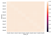
(a) The CKA similarity of IID with homo for stage 0.

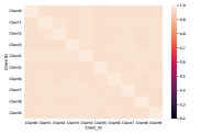
(b) The CKA similarity of IID with homo for stage 1.

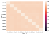
(c) The CKA similarity of IID with homo for stage 2.

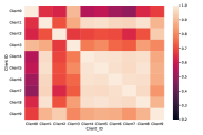
(d) The CKA similarity of IID with homo for stage 3.

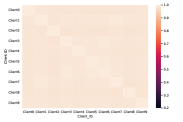
(e) The CKA similarity of Non-IID with homo for stage 0.

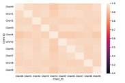
(f) The CKA similarity of Non-IID with homo for stage 1.

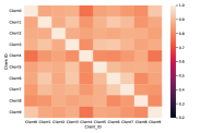
(g) The CKA similarity of Non-IID with homo for stage 2.

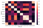
(h) The CKA similarity of Non-IID with homo for stage 3.

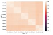
(i) The CKA similarity of Non-IID with hetero for stage 0.

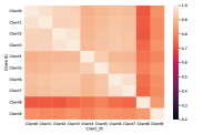
(j) The CKA similarity of Non-IID with hetero for stage 1.

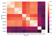
(k) The CKA similarity of Non-IID with hetero for stage 2.

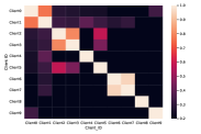
(l) The CKA similarity of Non-IID with hetero for stage 3.

Figure 12: The CKA similarity of IID with homo, Non-IID with homo and Non-IID with hetero for ResNets.

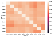
(a) The CKA similarity of IID with homo for layer 4.

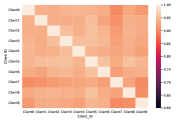
(b) The CKA similarity of IID with homo for layer 5.

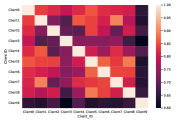
(c) The CKA similarity of IID with homo for layer 6.

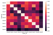
(d) The CKA similarity of IID with homo for layer 7.

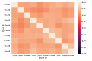
(e) The CKA similarity of Non-IID with homo for layer 4.

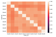
(f) The CKA similarity of Non-IID with homo for layer 5.

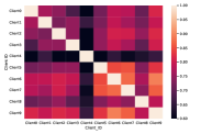
(g) The CKA similarity of Non-IID with homo for layer 6.

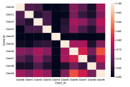
(h) The CKA similarity of Non-IID with homo for layer 7.

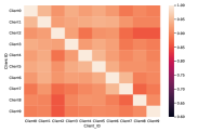
(i) The CKA similarity of Non-IID with hetero for layer 4.

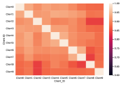
(j) The CKA similarity of Non-IID with hetero for layer 5.

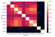
(k) The CKA similarity of Non-IID with hetero for layer 6.

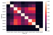
(l) The CKA similarity of Non-IID with hetero for layer 7.

Figure 13: The CKA similarity of IID with homo, Non-IID with homo and Non-IID with hetero for ViTs.

Appendix F More Details of the Experiments

F.1 Procedure for InCo Aggregation

The pseudo-codes for InCo Aggregation are shown in Algorithm 1. InCo Aggregation is operated in a server model, indicating that the methods focused on the client can be aligned with InCo Aggregation, as shown in our experiments.

Algorithm 1 InCo Aggregation (InCoAvg as the example)

1:Dataset $D_{k},k\in\{1,...,K\}$, $K$ clients, and their weights $w_{1},...,w_{K}$.

2:Weights for all clients $w_{1},...,w_{K}$.

3:Server process:

4:while not converge do

5:     Receives $g_{w_{i}}^{t}$ from the sampled client.

6:     Heterogeneous Aggregation for $g_{w_{i}}^{t}$.

7:     for each layer $l_{k}$ in the server model do

8:         if $l_{k}$ needs cross-layer gradients then

9:              ${g_{l_{k}}^{t}}^{\prime},{g_{l_{0}}^{t}}^{\prime}\leftarrow$Normalizes $g_{l_{k}}^{t}$ and $g_{l_{0}}^{t}$.

10:              $\theta^{t},\alpha,\beta$ from Theorem 3.1.

11:              $g_{l_{k}}^{t+1}=\frac{{(g_{l_{k}}^{t}}^{\prime}-\theta^{t}{g_{l_{0}}^{t}}^{\prime})\times({||g_{l_{k}}^{t}||+||g_{l_{0}}^{t}||})}{2}$.

12:         else

13:              $g_{l_{k}}^{t+1}=g_{l_{k}}^{t}$

14:         end if

15:         $w_{l_{k}}^{t+1}=w_{l_{k}}^{t}+g_{l_{k}}^{t+1}$

16:     end for

17:     Sends the updated $w_{i}^{t+1}$ to sampled clients.

18:end while

19:Client processes:

20:while random clients $i,i\in{1,...,K}$ do

21:     Receives model weights $w_{i}^{t-1}$.

22:     Updates client models $w_{i}^{t-1}$ to $w_{i}^{t}$.

23:     Sends $g_{w_{i}}^{t}=w_{i}^{t}-w_{i}^{t-1}$ to the server.

24:end while

F.2 Datasets

We conduct experiments on Fashion-MNIST, SVHN, CIFAR-10, and CINIC-10. CINIC-10 is a dataset of the mix of CIFAR-10 and ImageNet within ten classes. We use 3$\times$224$\times$224 with the ViT models and 3$\times$32$\times$32 with the ResNet models for all datasets.

F.3 Hyper-parameters

We use Adam optimizer with a learning rate of 0.001, $\beta_{1}=0.9$ and $\beta_{2}=0.999$, default parameter settings for all methods of ResNets. The local training epochs are fixed to 5. The batch size is 64 for all experiments. Furthermore, the global communication rounds are 500 for ResNets, and 200 for ViTs for all datasets. Global communication rounds for MOON and InCoMOON are 100 to prevent the extreme overfitting in Fashion-MNIST. The hyper-parameter $\frac{\mu}{2}$ for FedProx and InCoProx is 0.05 for ViTs and ResNets. We conduct our experiments with 4 NVIDIA GeForce RTX 3090s.

Table 4: Test accuracy of 100 clients and sample ratio 0.1. We shade in gray the methods that are combined with our proposed method, InCo Aggregation. We show the error bars for InCo Aggregation in this table.

Base	Methods	Fashion-MNIST		SVHN		CIFAR10		CINIC10
		$\alpha=0.5$	$\alpha=1.0$	$\alpha=0.5$	$\alpha=1.0$	$\alpha=0.5$	$\alpha=1.0$	$\alpha=0.5$	$\alpha=1.0$
ResNet	FedAvg	86.7$\pm$1.0	87.7$\pm$0.6	74.8$\pm$3.2	81.6$\pm$2.5	52.3$\pm$3.4	61.3$\pm$3.2	43.1$\pm$2.7	49.2$\pm$3.1
	FedProx	75.1$\pm$1.8	76.6$\pm$1.5	32.0$\pm$2.8	43.7$\pm$2.9	19.2$\pm$2.2	23.4$\pm$2.4	17.4$\pm$1.7	19.8$\pm$1.4
	Scaffold	87.9$\pm$0.5	88.0$\pm$0.3	76.3$\pm$3.4	82.4$\pm$3.1	54.3$\pm$3.6	61.8$\pm$3.0	43.5$\pm$2.4	49.4$\pm$3.1
	FedNova	12.7$\pm$0.2	15.6$\pm$0.2	13.4$\pm$ 0.4	15.3$\pm$0.3	10.4$\pm$0.3	14.3$\pm$0.2	12.0$\pm$0.3	14.0$\pm$0.2
	MOON	87.7$\pm$0.4	87.5$\pm$0.3	72.8$\pm$4.3	81.2$\pm$3.2	47.2$\pm$2.7	58.8$\pm$2.6	40.8$\pm$2.1	49.2$\pm$ 1.9
	InCoAvg	90.2$\pm$1.2	88.4$\pm$1.8	87.6$\pm$2.8	89.0$\pm$2.6	67.8$\pm$3.2	70.7$\pm$3.4	53.0$\pm$3.2	57.5$\pm$3.3
	InCoProx	88.8$\pm$2.3	86.4$\pm$3.2	89.0$\pm$1.3	90.8$\pm$1.2	74.5$\pm$2.3	76.8$\pm$1.8	59.1$\pm$3.2	62.5$\pm$2.4
	InCoScaffold	88.3$\pm$1.4	90.1$\pm$1.2	85.4$\pm$2.4	87.8$\pm$3.5	67.3$\pm$3.6	73.8$\pm$2.9	53.5$\pm$3.3	61.7$\pm$3.0
	InCoNova	86.6$\pm$1.4	87.4$\pm$1.3	86.4$\pm$2.5	88.4$\pm$1.8	62.8$\pm$3.9	69.7$\pm$4.2	48.0$\pm$2.7	54.1$\pm$1.7
	InCoMOON	89.1$\pm$1.3	89.5$\pm$1.2	85.6$\pm$3.8	89.3$\pm$2.0	68.2$\pm$3.1	71.8$\pm$2.3	54.3$\pm$3.0	57.6$\pm$2.7
ViT	FedAvg	92.0$\pm$0.7	91.9$\pm$0.5	92.4$\pm$0.9	93.9$\pm$0.8	93.7$\pm$1.0	94.2$\pm$0.8	83.8$\pm$1.4	85.1$\pm$0.9
	FedProx	89.8$\pm$0.5	89.7$\pm$0.5	71.4$\pm$3.8	81.1$\pm$2.9	82.6$\pm$3.3	84.7$\pm$2.3	67.8$\pm$2.8	71.3$\pm$3.0
	Scaffold	92.0$\pm$0.4	92.0$\pm$0.5	92.2$\pm$0.8	93.8$\pm$0.6	93.5$\pm$0.7	94.5$\pm$0.5	83.3$\pm$1.6	85.5$\pm$1.2
	FedNova	70.3$\pm$0.5	76.7$\pm$0.4	27.4$\pm$0.4	49.8$\pm$0.5	30.7$\pm$0.3	54.4$\pm$0.5	31.6$\pm$1.5	50.7$\pm$1.3
	MOON	92.1$\pm$0.3	92.1$\pm$0.2	92.5$\pm$1.2	93.9$\pm$0.9	93.6$\pm$0.8	94.6$\pm$0.3	84.3$\pm$1.6	85.3$\pm$1.2
	InCoAvg	93.0$\pm$0.6	93.1$\pm$0.5	94.2$\pm$0.6	95.0$\pm$0.4	94.6$\pm$0.7	95.0$\pm$0.6	85.9$\pm$1.9	86.8$\pm$1.3
	InCoProx	92.6$\pm$0.3	92.5$\pm$0.3	93.9$\pm$0.7	94.4$\pm$0.6	94.0$\pm$1.0	94.8$\pm$0.7	85.1$\pm$1.4	86.0$\pm$0.8
	InCoScaffold	92.9$\pm$0.3	93.0$\pm$0.2	94.0$\pm$1.1	94.8$\pm$0.6	94.6$\pm$0.5	95.0$\pm$0.2	85.7$\pm$1.3	86.5$\pm$1.1
	InCoNova	93.1$\pm$0.3	93.6$\pm$0.3	94.7$\pm$0.9	95.6$\pm$0.5	94.8$\pm$0.4	95.7$\pm$0.3	86.2$\pm$1.8	88.2$\pm$1.0
	InCoMOON	92.8$\pm$0.5	93.0$\pm$0.3	94.7$\pm$0.8	95.1$\pm$0.5	94.2$\pm$0.8	95.1$\pm$0.5	86.0$\pm$0.9	86.8$\pm$1.3

F.4 Error Bars of InCo Aggregation

We illustrate the error bars of InCo Aggregation in Table 4. These results show the stability of InCo Aggregation. In all cases of ResNets and many cases of ViTs, the worst results of InCo Aggregation are better than the Averaging Aggregation, demonstrating the efficacy of InCo Aggregation.

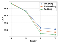
(a) CIFAR10 with $\alpha=0.5$.

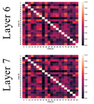
(b) InCoAvg.

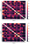
(c) HeteroAvg.

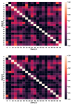
(d) FedAvg.

Figure 14: CKA layer similarity and Heatmaps of ViTs. (a): The layer similarity of different methods. (b) to (d): Heatmaps for different methods in layer 6 and layer 7.

F.5 Layer Similarity and Heatmaps of ViTs

Figure 14 illustrates the layer similarity of the last four layers, along with the corresponding heatmaps for Layer 6 and Layer 7. Furthermore, Figure 14a demonstrates that InCo Aggregation significantly enhances the layer similarity, validating the initial motivation behind our proposed method. Additionally, since the disparity in layer similarity between Layer 6 and Layer 7 is minimal, the heatmaps for these layers do not exhibit significant differences, as depicted in Figure 14b through Figure 14d.

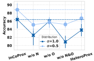
(a) Fashion-MNIST.

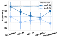
(b) SVHN.

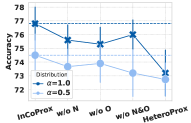
(c) CIFAR-10.

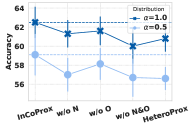
(d) CINIC-10.

Figure 15: Ablation studies for InCo Aggregation for FedProx. The federated settings are the same as Table 2.

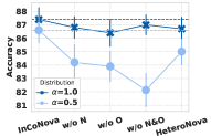
(a) Fashion-MNIST.

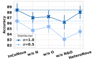
(b) SVHN.

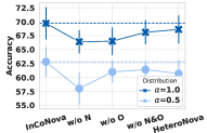
(c) CIFAR-10.

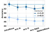
(d) CINIC-10.

Figure 16: Ablation studies for InCo Aggregation for FedNova. The federated settings are the same as Table 2.

F.6 More Ablation Studies and Robustness Analysis.

We conduct additional experiments on different baselines to demonstrate the effectiveness of InCo Aggregation. Figure 15 to Figure 17 present the results of the ablation study for FedProx, FedNova, and Scaffold, incorporating InCo Aggregation. These results highlight the efficacy of InCo Aggregation across different baselines. Additionally, Figure 18 and Figure 19 illustrate the robustness analysis for FedProx and Scaffold. In Figure 18, we observe that FedProx faces challenges in achieving convergence in all settings, whereas InCoProx exhibits great results with significant improvements over FedProx. In Figure 19, InCoScaffold consistently obtains the best performances across all settings. These experiments provide further evidence of the efficiency of InCo Aggregation.

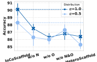
(a) Fashion-MNIST.

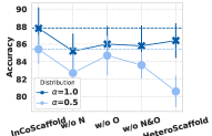
(b) SVHN.

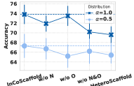
(c) CIFAR-10.

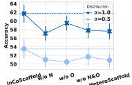
(d) CINIC-10.

Figure 17: Ablation studies for InCo Aggregation for Scaffold. The federated settings are the same as Table 2.

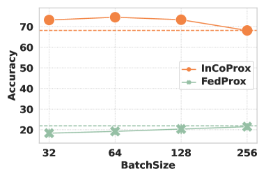
(a) Different batch sizes.

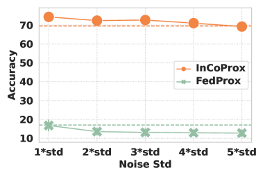
(b) Different noise perturbations.

Figure 18: Robustness analysis for InCo Aggregation for FedProx in CIFAR-10.

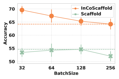
(a) Different batch sizes.

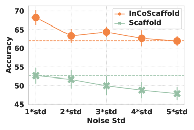
(b) Different noise perturbations.

Figure 19: Robustness analysis for InCo Aggregation for Scaffold in CIFAR-10.

References

- (1) Samiul Alam, Luyang Liu, Ming Yan, and Mi Zhang. Fedrolex: Model-heterogeneous federated learning with rolling sub-model extraction. In Advances in Neural Information Processing Systems, 2022.
- (2) Hankyul Baek, Won Joon Yun, Yunseok Kwak, Soyi Jung, Mingyue Ji, Mehdi Bennis, Jihong Park, and Joongheon Kim. Joint superposition coding and training for federated learning over multi-width neural networks. In IEEE INFOCOM 2022-IEEE Conference on Computer Communications, pages 1729–1738. IEEE, 2022.
- (3) Radu Ioan Bot, Sorin-Mihai Grad, and Gert Wanka. Duality in vector optimization. Springer Science & Business Media, 2009.
- (4) Stephen Boyd, Stephen P Boyd, and Lieven Vandenberghe. Convex optimization. Cambridge university press, 2004.
- (5) Sebastian Caldas, Jakub Konečny, H Brendan McMahan, and Ameet Talwalkar. Expanding the reach of federated learning by reducing client resource requirements. arXiv preprint arXiv:1812.07210, 2018.
- (6) Yun Hin Chan and Edith Ngai. Fedhe: Heterogeneous models and communication-efficient federated learning. IEEE International Confer- ence on Mobility, Sensing and Networking (MSN 2021), 2021.
- (7) Yun-Hin Chan and Edith C. H. Ngai. Exploiting features and logits in heterogeneous federated learning, 2022.
- (8) Chen Chen, Hong Xu, Wei Wang, Baochun Li, Bo Li, Li Chen, and Gong Zhang. Communication-efficient federated learning with adaptive parameter freezing. In 2021 IEEE 41st International Conference on Distributed Computing Systems (ICDCS), pages 1–11. IEEE, 2021.
- (9) Hanting Chen, Yunhe Wang, Chang Xu, Zhaohui Yang, Chuanjian Liu, Boxin Shi, Chunjing Xu, Chao Xu, and Qi Tian. Data-free learning of student networks. In Proceedings of the IEEE/CVF International Conference on Computer Vision, pages 3514–3522, 2019.
- (10) Luke N Darlow, Elliot J Crowley, Antreas Antoniou, and Amos J Storkey. Cinic-10 is not imagenet or cifar-10. arXiv preprint arXiv:1810.03505, 2018.
- (11) Enmao Diao, Jie Ding, and Vahid Tarokh. HeteroFL: Computation and communication efficient federated learning for heterogeneous clients. In International Conference on Learning Representations, 2021.
- (12) Alexey Dosovitskiy, Lucas Beyer, Alexander Kolesnikov, Dirk Weissenborn, Xiaohua Zhai, Thomas Unterthiner, Mostafa Dehghani, Matthias Minderer, Georg Heigold, Sylvain Gelly, et al. An image is worth 16x16 words: Transformers for image recognition at scale. arXiv preprint arXiv:2010.11929, 2020.
- (13) Xiuwen Fang and Mang Ye. Robust federated learning with noisy and heterogeneous clients. In Proceedings of the IEEE/CVF Conference on Computer Vision and Pattern Recognition, pages 10072–10081, 2022.
- (14) Dashan Gao, Xin Yao, and Qiang Yang. A survey on heterogeneous federated learning, 2022.
- (15) Ian Goodfellow, Jean Pouget-Abadie, Mehdi Mirza, Bing Xu, David Warde-Farley, Sherjil Ozair, Aaron Courville, and Yoshua Bengio. Generative adversarial nets. Advances in neural information processing systems, 27, 2014.
- (16) Chaoyang He, Murali Annavaram, and Salman Avestimehr. Group knowledge transfer: Federated learning of large cnns at the edge. Advances in Neural Information Processing Systems, 33:14068–14080, 2020.
- (17) Kaiming He, Xiangyu Zhang, Shaoqing Ren, and Jian Sun. Identity mappings in deep residual networks. In Computer Vision–ECCV 2016: 14th European Conference, Amsterdam, The Netherlands, October 11–14, 2016, Proceedings, Part IV 14, pages 630–645. Springer, 2016.
- (18) Geoffrey Hinton, Oriol Vinyals, and Jeff Dean. Distilling the knowledge in a neural network. NIPS Deep Learning and Representation Learning Workshop, 2015.
- (19) Sepp Hochreiter and Jürgen Schmidhuber. Long short-term memory. Neural computation, 9(8):1735–1780, 1997.
- (20) Samuel Horvath, Stefanos Laskaridis, Mario Almeida, Ilias Leontiadis, Stylianos Venieris, and Nicholas Lane. Fjord: Fair and accurate federated learning under heterogeneous targets with ordered dropout. Advances in Neural Information Processing Systems, 34:12876–12889, 2021.
- (21) Wenke Huang, Mang Ye, and Bo Du. Learn from others and be yourself in heterogeneous federated learning. In Proceedings of the IEEE/CVF Conference on Computer Vision and Pattern Recognition, pages 10143–10153, 2022.
- (22) Yangsibo Huang, Samyak Gupta, Zhao Song, Kai Li, and Sanjeev Arora. Evaluating gradient inversion attacks and defenses in federated learning. Advances in Neural Information Processing Systems, 34:7232–7241, 2021.
- (23) Wonyong Jeong and Sung Ju Hwang. Factorized-fl: Personalized federated learning with parameter factorization & similarity matching. In Advances in Neural Information Processing Systems, 2022.
- (24) Peter Kairouz, H Brendan McMahan, Brendan Avent, Aurélien Bellet, Mehdi Bennis, Arjun Nitin Bhagoji, Kallista Bonawitz, Zachary Charles, Graham Cormode, Rachel Cummings, et al. Advances and open problems in federated learning. 2021.
- (25) Sai Praneeth Karimireddy, Satyen Kale, Mehryar Mohri, Sashank Reddi, Sebastian Stich, and Ananda Theertha Suresh. Scaffold: Stochastic controlled averaging for federated learning. In International Conference on Machine Learning, pages 5132–5143. PMLR, 2020.
- (26) Diederik P. Kingma and Jimmy Ba. Adam: A method for stochastic optimization. In Yoshua Bengio and Yann LeCun, editors, 3rd International Conference on Learning Representations, ICLR 2015, San Diego, CA, USA, May 7-9, 2015, Conference Track Proceedings, 2015.
- (27) Simon Kornblith, Mohammad Norouzi, Honglak Lee, and Geoffrey Hinton. Similarity of neural network representations revisited. In International Conference on Machine Learning, pages 3519–3529. PMLR, 2019.
- (28) Alex Krizhevsky, Geoffrey Hinton, et al. Learning multiple layers of features from tiny images. 2009.
- (29) Daliang Li and Junpu Wang. FedMD: Heterogenous federated learning via model distillation. NeurIPS Workshop on Federated Learning for Data Privacy and Confidentiality, 2019.
- (30) Qinbin Li, Yiqun Diao, Quan Chen, and Bingsheng He. Federated learning on non-iid data silos: An experimental study. In 2022 IEEE 38th International Conference on Data Engineering (ICDE), pages 965–978. IEEE, 2022.
- (31) Qinbin Li, Bingsheng He, and Dawn Song. Model-contrastive federated learning. In Proceedings of the IEEE/CVF Conference on Computer Vision and Pattern Recognition, pages 10713–10722, 2021.
- (32) Tian Li, Anit Kumar Sahu, Ameet Talwalkar, and Virginia Smith. Federated learning: Challenges, methods, and future directions. IEEE Signal Processing Magazine, 37(3):50–60, 2020.
- (33) Tian Li, Anit Kumar Sahu, Manzil Zaheer, Maziar Sanjabi, Ameet Talwalkar, and Virginia Smith. Federated optimization in heterogeneous networks. Proceedings of the 3rd MLSys Conference, 2020.
- (34) Yiying Li, Wei Zhou, Huaimin Wang, Haibo Mi, and Timothy M Hospedales. FedH2L: Federated learning with model and statistical heterogeneity. arXiv preprint arXiv:2101.11296, 2021.
- (35) Tao Lin, Lingjing Kong, Sebastian U Stich, and Martin Jaggi. Ensemble distillation for robust model fusion in federated learning. Advances in Neural Information Processing Systems, 33:2351–2363, 2020.
- (36) Ruixuan Liu, Fangzhao Wu, Chuhan Wu, Yanlin Wang, Lingjuan Lyu, Hong Chen, and Xing Xie. No one left behind: Inclusive federated learning over heterogeneous devices. In Proceedings of the 28th ACM SIGKDD Conference on Knowledge Discovery and Data Mining, pages 3398–3406, 2022.
- (37) Kevin Lu, Aditya Grover, Pieter Abbeel, and Igor Mordatch. Pretrained transformers as universal computation engines. arXiv preprint arXiv:2103.05247, 1, 2021.
- (38) Mi Luo, Fei Chen, Dapeng Hu, Yifan Zhang, Jian Liang, and Jiashi Feng. No fear of heterogeneity: Classifier calibration for federated learning with non-iid data. Advances in Neural Information Processing Systems, 34:5972–5984, 2021.
- (39) Brendan McMahan, Eider Moore, Daniel Ramage, Seth Hampson, and Blaise Aguera y Arcas. Communication-efficient learning of deep networks from decentralized data. In Artificial intelligence and statistics, pages 1273–1282. PMLR, 2017.
- (40) Mehryar Mohri, Gary Sivek, and Ananda Theertha Suresh. Agnostic federated learning. In International Conference on Machine Learning, pages 4615–4625. PMLR, 2019.
- (41) Gaurav Kumar Nayak, Konda Reddy Mopuri, Vaisakh Shaj, Venkatesh Babu Radhakrishnan, and Anirban Chakraborty. Zero-shot knowledge distillation in deep networks. In International Conference on Machine Learning, pages 4743–4751. PMLR, 2019.
- (42) Yuval Netzer, Tao Wang, Adam Coates, Alessandro Bissacco, Bo Wu, and Andrew Y Ng. Reading digits in natural images with unsupervised feature learning. 2011.
- (43) Maithra Raghu, Thomas Unterthiner, Simon Kornblith, Chiyuan Zhang, and Alexey Dosovitskiy. Do vision transformers see like convolutional neural networks? Advances in Neural Information Processing Systems, 34:12116–12128, 2021.
- (44) Sebastian Ruder. An overview of gradient descent optimization algorithms. arXiv preprint arXiv:1609.04747, 2016.
- (45) Felix Sattler, Tim Korjakow, Roman Rischke, and Wojciech Samek. Fedaux: Leveraging unlabeled auxiliary data in federated learning. IEEE Transactions on Neural Networks and Learning Systems, 2021.
- (46) Tao Shen, Jie Zhang, Xinkang Jia, Fengda Zhang, Gang Huang, Pan Zhou, Kun Kuang, Fei Wu, and Chao Wu. Federated mutual learning. arXiv preprint arXiv:2006.16765, 2020.
- (47) Yue Tan, Guodong Long, Lu Liu, Tianyi Zhou, Qinghua Lu, Jing Jiang, and Chengqi Zhang. Fedproto: Federated prototype learning across heterogeneous clients. In Proceedings of the AAAI Conference on Artificial Intelligence, volume 36, pages 8432–8440, 2022.
- (48) Laurens Van der Maaten and Geoffrey Hinton. Visualizing data using t-sne. Journal of machine learning research, 9(11), 2008.
- (49) Jianyu Wang, Qinghua Liu, Hao Liang, Gauri Joshi, and H Vincent Poor. Tackling the objective inconsistency problem in heterogeneous federated optimization. Advances in neural information processing systems, 33:7611–7623, 2020.
- (50) Han Xiao, Kashif Rasul, and Roland Vollgraf. Fashion-MNIST: a novel image dataset for benchmarking machine learning algorithms, 2017.
- (51) Cong Xie, Sanmi Koyejo, and Indranil Gupta. Asynchronous federated optimization. 12th Annual Workshop on Optimization for Machine Learning, 2020.
- (52) Jiahui Yu and Thomas S Huang. Universally slimmable networks and improved training techniques. In Proceedings of the IEEE/CVF international conference on computer vision, pages 1803–1811, 2019.
- (53) Yue Zhao, Meng Li, Liangzhen Lai, Naveen Suda, Damon Civin, and Vikas Chandra. Federated learning with non-iid data. arXiv preprint arXiv:1806.00582, 2018.
- (54) Zhuangdi Zhu, Junyuan Hong, and Jiayu Zhou. Data-free knowledge distillation for heterogeneous federated learning. In International Conference on Machine Learning, pages 12878–12889. PMLR, 2021.