Bridging Cognitive Maps: a Hierarchical Active Inference Model of Spatial Alternation Tasks and the Hippocampal-Prefrontal Circuit

Abstract

Cognitive problem-solving benefits from cognitive maps aiding navigation and planning. Previous studies revealed that cognitive maps for physical space navigation involve hippocampal (HC) allocentric codes, while cognitive maps for abstract task space engage medial prefrontal cortex (mPFC) task-specific codes. Solving challenging cognitive tasks requires integrating these two types of maps. This is exemplified by spatial alternation tasks in multi-corridor settings, where animals like rodents are rewarded upon executing an alternation pattern in maze corridors. Existing studies demonstrated the HC – mPFC circuit’s engagement in spatial alternation tasks and that its disruption impairs task performance. Yet, a comprehensive theory explaining how this circuit integrates task-related and spatial information is lacking. We advance a novel hierarchical active inference model clarifying how the HC – mPFC circuit enables the resolution of spatial alternation tasks, by merging physical and task-space cognitive maps. Through a series of simulations, we demonstrate that the model’s dual layers acquire effective cognitive maps for navigation within physical (HC map) and task (mPFC map) spaces, using a biologically-inspired approach: a clone-structured cognitive graph. The model solves spatial alternation tasks through reciprocal interactions between the two layers. Importantly, disrupting inter-layer communication impairs difficult decisions, consistent with empirical findings. The same model showcases the ability to switch between multiple alternation rules. However, inhibiting message transmission between the two layers results in perseverative behavior, consistent with empirical findings. In summary, our model provides a mechanistic account of how the HC – mPFC circuit supports spatial alternation tasks and how its disruption impairs task performance.

[idlab] organization=IDLab, Department of Information Technology, Ghent University - imec, city=Ghent, country=Belgium [verses] organization=VERSES Research Lab, city=Los Angeles, country=USA [istc] organization=Institute of Cognitive Sciences and Technologies, National Research Council, city=Rome, country=Italy

Highlights

• Hierarchical active inference model of spatial alternation tasks

• The model integrates cognitive maps of task and physical space

• Both maps are learned using clone-structured cognitive graphs

• The integrated model reproduces key functions of the hippocampal - prefrontal circuit

• Model disruptions impair spatial alternation tasks, reproducing empirical findings

1 Introduction

To solve cognitive problems, such as finding the shortest route to a goal destination in a busy city, we can use so-called cognitive maps of the situation that affords flexible planning. The concept of the cognitive map has been initially popularized by Tolman, especially in the context of spatial navigation (Tolman,, 1948). An extensive body of literature has investigated the neuronal underpinnings of cognitive maps for spatial navigation in humans, rodents, and other animals. This research has established the crucial importance of structures of the medial temporal lobe and especially of the hippocampal formation in the creation of codes for allocentric space, such as place cells (in the hippocampus) (O’Keefe and Nadel,, 1979; O’Keefe and Dostrovsky,, 1971) and grid cells (in the entorhinal cortex) (Hafting et al.,, 2005). The same brain structures might provide a geometric code to navigate in “cognitive” domains, too (Bellmund et al.,, 2018; Epstein et al.,, 2017; Buzsáki and Moser,, 2013).

In parallel, the concept of a cognitive map can apply to more abstract state spaces that describe the sequential stages of a task at hand (for example, buying a gift in one’s preferred shop and then bringing it to a friend’s house) as opposed to the more fine-grained spatial codes found in the hippocampal formation. Recent studies reported that prefrontal structures, such as the orbitofrontal cortex, might host such coarse task codes, which might permit representing (for example) the current and the next stages of the task (Niv,, 2019; Schuck et al.,, 2016) as well as future navigational goals (Basu et al.,, 2021), as opposed to a physical location.

Crucially, during goal-directed spatial navigation (and other cognitive problems), it is often necessary to combine cognitive maps of task space (to find a sequence of coarse-grained actions to progress in task space, such as ensuring the correct sequence of destinations to buy and deliver a gift) and physical space (to find a path that reaches the next intended destination) (Ito et al.,, 2015; Pezzulo et al.,, 2014; Verschure et al.,, 2014). However, we still lack a comprehensive theory that explains the ways cognitive maps of physical and task space interact when executing cognitive tasks.

A useful starting point to understand the interaction of task-related and spatial codes is rodent memory-guided, spatial alternation tasks. A prominent example is the spatial alternation task in the W-maze studied in (Jadhav et al.,, 2012). As visualized in Figure 1, the W-maze comprises three corridors. To collect rewards, the animal has to visit the corridors in the correct order, according to an “alternation rule” (e.g. left, center, right, center, left, etc) that is initially unknown and has to be learned by trial and error.

A series of experiments showed that solving the spatial alternation task engages coordinated patterns of neural activity in the hippocampus (HC), which putatively encodes the spatial aspects of the task, and the prefrontal cortex (mPFC), which putatively learns the alternation rule and uses it to guide behavior (Benchenane et al.,, 2011; Shin and Jadhav,, 2016; Colgin,, 2011; Siapas et al.,, 2005; Khodagholy et al.,, 2017). For example, the HC - mPFC interaction is selectively enhanced during epochs requiring spatial working memory (Jones and Wilson,, 2005). Furthermore, the coordination of neural activity in both structures spans multiple timescales, from theta sequences during navigation to reactivation (replay) activity during inter-trial periods prior to navigation – and is considered crucial for the information exchange between the two areas during the task (Tang et al.,, 2021).

Notably, disrupting awake hippocampal reactivations (sharp wave ripples, SWR) at decision points impaired the animal’s performance, but only for the aspects of the alternation task that require spatial working memory (Jadhav et al.,, 2012), see Figure 1. Specifically, disrupting awake SWRs impaired outbound decisions (from the central corridor to the left or right corridor), which require memory for immediate past outer arm location. Rather, the same SWR disruption did not impair inbound decisions (from the left or right corridor to the central corridor) that do not require memory of the past corridor; nor did it impair self-localization (Jadhav et al.,, 2012). The study concludes that impairing SWRs prevents the hippocampus from providing information about past locations (and/or future options) to the prefrontal cortex, which is responsible to learn the alternation rule and to use it to guide behavior. In other words, the SWR disruption impairs communication between the hippocampus and the prefrontal cortex, hence preventing the latter from correctly inferring the current stage in task space.

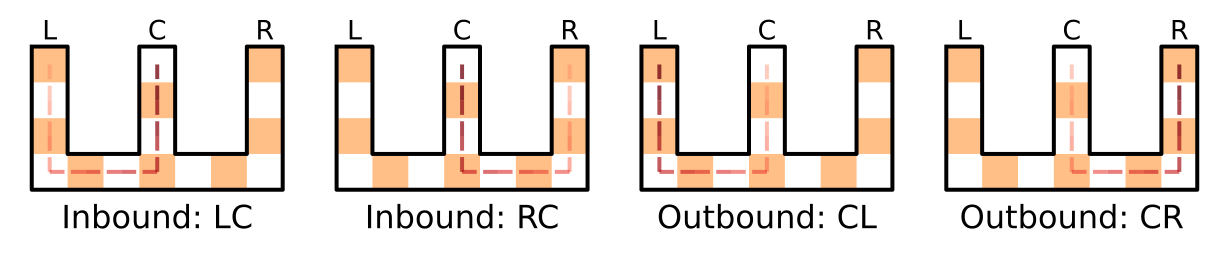
((a))

Figure 1: Spatial alternation tasks (LCRC). This figure exemplifies the W-maze used in  (Jadhav et al.,, 2012) to study spatial alternation and the role of the hippocampal - prefrontal dynamics. The W-maze is characterized by three separate corridors. The animal can acquire the reward at the end of each corridor, however, to receive the reward it must do so in the correct order (e.g. Left, Center, Right, Center, Left, etc). The spatial alternation task implies that when the animal is in the center position, it has to make a (difficult) outbound decision: it has to go either to the left or the right, depending on where it comes from. This outbound decision, therefore, requires a spatial memory component. In contrast, when the animal is in one of the side corridors (left or right), the only correct action is to move to the center. This inbound decision is considered simpler since it does not require a memory component. Trajectory order is indicated by the shade where lighter is earlier.

The importance of hippocampal-prefrontal communication for memory guided decisions is confirmed by another study in which animals had to learn and subsequently switch between three spatial alternation rules in the same three-arm maze  (Den Bakker et al.,, 2022). This study showed that disrupting neural activity in the mPFC directly following hippocampal sharp-wave ripples (but not after a random delay) impairs the animal’s ability to switch between learned rules.

Here, we advance a novel computational theory that casts the interactions between the hippocampus (HC) and the medial prefrontal cortex (mPFC) during spatial alternation tasks, in terms of hierarchical active inference (Friston,, 2010; Friston et al., 2017a, ; Bogacz,, 2017; Buckley et al.,, 2017; Parr et al.,, 2022; Smith et al.,, 2022; Isomura et al.,, 2023). Our theory has two main tenets. First, the HC and the mPFC learn cognitive maps for navigation in physical and task space, respectively, using the same statistical computations, but based on different inputs (see Section 4). Second, the neural circuit formed by the HC and the mPFC realizes a hierarchical active inference architecture, which can solve spatial alternation tasks. Hierarchical active inference rests on reciprocal, bottom-up, and top-down message passing. In the bottom-up pathway, the lower hierarchical level (encoding the HC map) infers the current location based on sensory information and communicates it to the higher level (encoding the mPFC map). In turn, the higher level infers the next goal location (in the mPFC map) and sets it as a goal for spatial navigation (in the HC map), in a top-down manner. Impairments of the message passing prevent the architecture from correctly solving spatial alternation tasks.

We exemplify the new theory by presenting two simulations of rodent spatial alternation tasks, with intact and impaired HC- mPFC interactions  (Jadhav et al.,, 2012; Den Bakker et al.,, 2022). Our first simulation, presented in Section 2.2, brings three main conclusions. First, the model is able to learn the spatial structure of the maze (HC map) and spatial alternation rules (mPFC) by navigating in the environment. Second, when the HC - mPFC circuit is configured as a hierarchical active inference system, it effectively solves spatial alternation tasks, through bottom-up and top-down message passing. Third, disrupting the interaction from the HC to the mPFC breaks the spatial memory and impairs the animal’s ability to make outbound but not inbound decisions, as observed empirically (Jadhav et al.,, 2012). Our second simulation, presented in Section 2.2.1, shows two additional features of the model. First, in a task in which three alternative spatial alternation rules are in play, the HC - mPFC circuit permits inferring the current rule. Second, selectively inhibiting the mPFC impairs this ability and provokes perseveration, as observed empirically in the study reported in (Den Bakker et al.,, 2022).

2 Results

2.1 The W-maze setup and the hierarchical active inference (HAI) agent

In this work, we consider the spatial alternation task in the W-maze of (Jadhav et al.,, 2012), see Figure 1. In this task, an animal (or an artificial agent) can acquire rewards at the end of each corridor, providing that the corridors are visited in the correct order (e.g. left, center, right, center, left).

In this section, we present a hierarchical active inference (HAI) agent (Parr et al.,, 2022) for solving the spatial alternation task. Central to this framework is the fact that agents are endowed with a generative model, describing how observed outcomes are generated from a hidden, unobserved state, which is influenced by the agent’s actions. The agent infers these hidden states by minimizing the free energy functional with respect to its belief over the state and acts to minimize its expected free energy over time (Parr et al.,, 2022). For more details on these mechanisms, the reader is referred to Section 4.2.

In our simulations, the HAI agent is endowed with a hierarchical generative model of two layers, which is schematically illustrated in Figure 2(b) (see Section 4.2 for a formal introduction). In this generative model, the lowest layer takes up the functional role of the hippocampus, namely encoding the spatial structure of the maze (O’Keefe and Nadel,, 1979). In contrast, the highest layer takes the functional role of the prefrontal cortex, namely encoding the structure of task space (Schuck et al.,, 2016). The agent learns both maps using the same sequence learning algorithm: the clone structured cognitive graphs (CSCG (George et al.,, 2021)), see Section 4 for details. The latent states learned by the CSCG at the two levels are schematically illustrated within the two boxes of Figure 2(b).

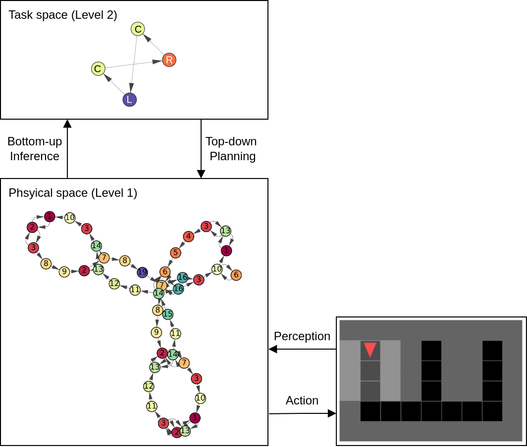
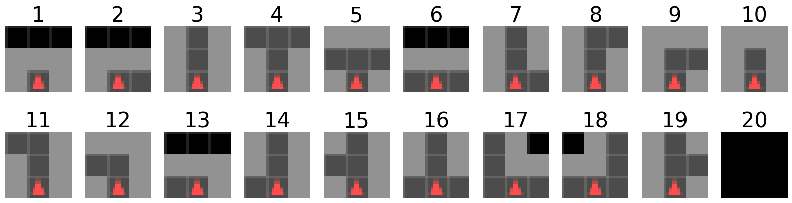
((a))

((b))

Figure 2: Illustration of the hierarchical active inference (HAI) agent and the W-maze setup (a) The hierarchical generative model of the HAI agent. The figure shows that the two layers of the model include cognitive maps of physical space (level 1) and task space (level 2). These cognitive maps essentially represent transitions between learned locations and stages of the task, respectively. Both maps are learned using a probabilistic sequence learning algorithm: the clone structured cognitive graph (CSCG (George et al.,, 2021)). Within each block, a subset of states from the CSCG is visualized, namely, the active states when pursuing the alternation rule (LCRC). For a visualization of the full set of states from the CSCG, we refer to Figure 5. The dynamics between the physical (level 1) and task space (level 2) CSCG in the hierarchical model are regulated by bottom-up message passing (that supports inference) and top-down message passing (that supports planning). Bottom-up inference messages from the physical space model are passed to the task space model, while top-down actions drive planning from the task-space model to the physical space model. An essential aspect of these interactions is that the two levels operate on a different temporal scale. Transitions at the physical level, through the agent’s movement, occur at every time step. Rather, the task level only transitions when the intermediate goal (of reaching a certain position in the maze) is achieved. This abstraction allows for hierarchical planning. Finally, the interaction with the environment using an action-perception loop with the world, the W-maze, is shown on the right. (b) The 20 distinct observations the agent can encounter in the W-maze created in the Minigrid environment (Chevalier-Boisvert et al.,, 2018).

Crucially, the HAI agent performs inference (of where it is in physical space, i.e., its pose, and in task space) and planning (of the next goal in physical and task space) through message-passing between the two hierarchical levels. As shown in Figure 2(b), level 1 observes the structural aspects of the environment through its bottom-up observations, i.e. the three-by-three grid around the agent as shown in Figure 2(b) and selects local movements in physical space such as “turn left”, “turn right” or “move forward” to reach any goal location (which is fed by the highest level, see below).

Once level 1 has navigated towards its local goal, it passes a bottom-up message containing the current state of the agent to level 2. In turn, level 2 processes this message and infers the next stage of the task to achieve a reward (as it is endowed with a prior preference to achieve reward at each step, see Section 4.2). Actions at level 2 are abstract and are matched to the bottom-up received observable states from level 1. Since level 1 states encode the agent’s pose, these actions essentially mean “move to target location”. We specifically encode only actions corresponding to target locations at the end of a corridor (i.e. observation 1 in Figure 2(b)). The selected action is sent to level 1 in a top-down manner and corresponds to the goal location for level 1. Once level 1 reaches the goal location, this process repeats.

Finally, the right part of Figure 2(b) illustrates the fact that the lowest level of the model is responsible for the action-perception loop with the environment – here, an implementation of the W-maze in the Minigrid (Chevalier-Boisvert et al.,, 2018) simulator. Observations in the Minigrid (Chevalier-Boisvert et al.,, 2018) are acquired as a square around the agent. In this work, we chose a range of three, yielding three-by-three observations which are then mapped to a unique one-hot index. For each step, the agent also observes a binary value indicating the reward presence. The actions the agent can perform are “turn left”, “turn right” and “move forward”, which are also represented as a one-hot index. See Section 4.2 for more details on the model implementation

2.2 Experiment 1: Solving the spatial alternation task

We replicate the task and experiment from a study on rodents (Jadhav et al.,, 2012) where the animal is taught this specific alternation task. In this study, disruption of the hippocampal sharp-wave ripple (SWR) reduces the performance on outbound trajectories, but not on inbound trajectories.

We first allow the HAI agent to learn the two cognitive maps for solving the spatial alternation task, using two CSCGs (see (George et al.,, 2021) and Section 4 for details on the learning procedure). The learned maps for the W-maze are shown within the two boxes of Figure 2(b). For ease of visualization, within each box, only a subset of states from the CSCG is shown, namely, the states that are active when correctly pursuing the alternation rule (the complete learned maps are shown in Figure 5). We denote the sequence of this alternation rule as LCRC (for Left, Center, Right, Center). For a visualization of the full set of states from the CSCG, please see Figure 5.

The hippocampal map on the lowest level organizes the 20 observations that the agent encounters during navigation (illustrated in Figure 2(b)) into a coherent graph, which nicely reflects the 3 corridors of the W-maze. In this map, the circles reflect the states learned by the CSCG, while the transitions reflect the agent’s spatial actions (e.g., “turn left”, “turn right”, or “move forward”). The nodes are color-coded (and numbered) according to the observations that they encode. Note that while the agent encounters the same observations multiple times during navigation (i.e., the observations are aliased), the CSCG correctly reflects the fact that they are part of different behavioral sequences. For example, observation 1 (that corresponds to the location in which a reward can be collected) appears three times, at the apex of each of the latent sequences that represent each of the three corridors.

The prefrontal map on the highest level corresponds to a much smaller graph that encodes the task-specific sequence of corridors that the agent has to visit to secure rewards. In this graph, the nodes correspond to (color-coded) corridors in which rewards have been collected and the edges correspond to higher-order actions (“go to corridor”). Note that there are nodes of the same color: both correspond to the central corridor but in different phases in task space (i.e., after the left and the right corridors, respectively). This indicates that the agent has successfully learned a low-dimensional representation of (or a finite state machine for) the task rule LCRC.

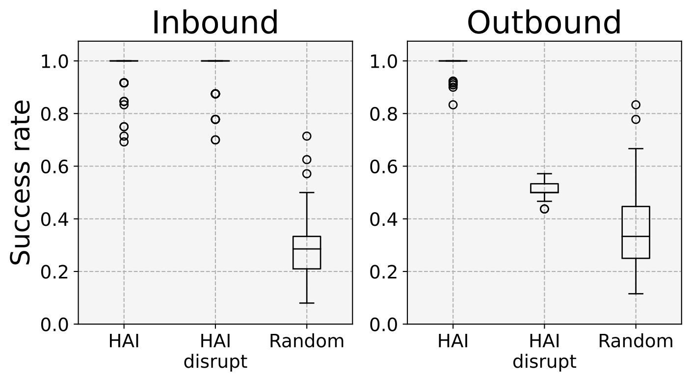
((a))

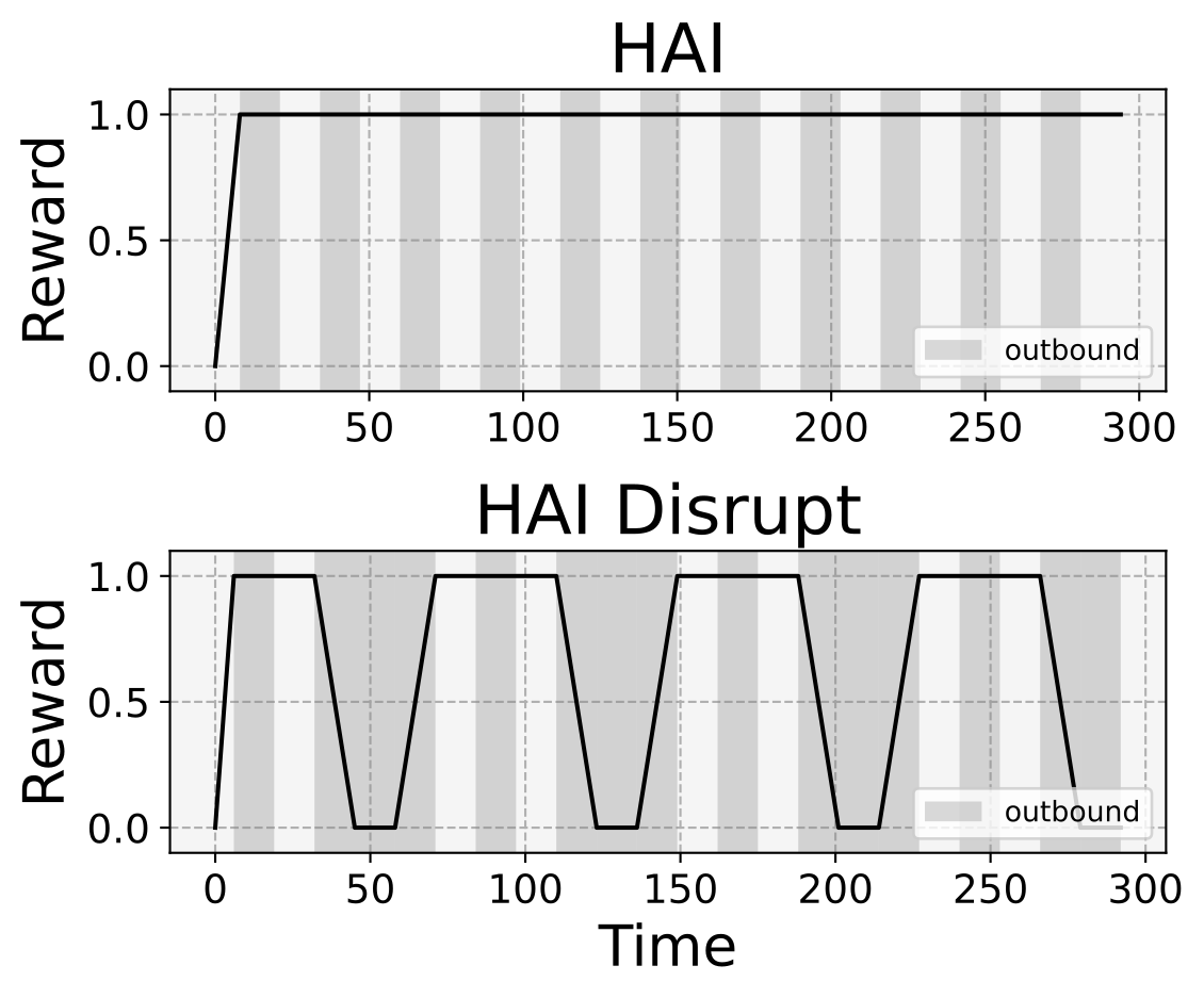
((b))

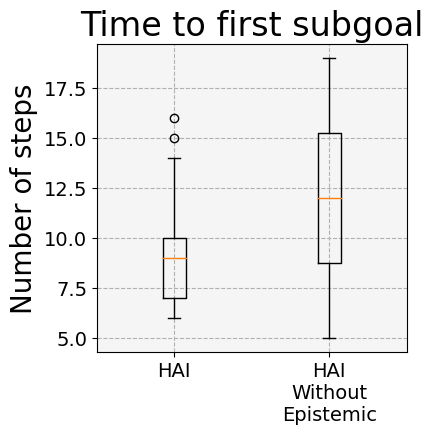
((c))

Figure 3: Experiment 1: Solving the spatial alternation task with intact and disrupted spatial memory. (a) The success rate in the spatial alternation task for the HAI agent without disruption, the HAI agent with disruption (HAI disrupted), and the Random agent, separated for both in- and outbound trajectories. The success rate is computed over 100 trials per agent, with 300 steps per trial, only recording the presence of reward at the end of the selected corridors. (b) The reward over time for the HAI agent and a disrupted HAI agent. The shaded areas in the plot indicate outbound trajectories. (c) A comparison of the performance (time to reach the first subgoal) of the HAI agent and a variant of the HAI agent, which selects actions based on reward optimization (pragmatic imperative of active inference) but not uncertainty reduction (epistemic imperative of active inference).

We then investigate whether the HAI agent equipped with the learned cognitive maps for physical and task space is able to solve spatial alternation tasks. For this, we endow the HAI agent with a prior preference for maximizing the reward and place it in a random pose in the W-maze. We then let the agent run for 300 steps, and record whether it selected the correct or the incorrect corridor to find the reward. We repeat this experiment for 100 trials, to collect statistics. Figure 3(a) shows that the HAI agent has near-perfect performance during both inbound and outbound decisions; furthermore, as expected, it significantly outperforms a Random agent that selects the next corridor randomly (t-test p=0). Figure 3(b) shows that after a few time steps, once the HAI agent has inferred where it is (in both physical and task space), it consistently follows the rule and is able to collect rewards at every step.

Finally, figure 3(c) provides a more fine-grained illustration of the strategy used by the HAI agent to solve the task. During the task, the HAI agent selects its actions based on both a pragmatic imperative (to reach the next subgoal to secure reward) and an epistemic imperative (to reduce its uncertainty about its current pose, by going to places where unambiguous observations could be found, e.g., the T-junction). Both the pragmatic and the epistemic imperative are part and parcel of the expected free energy functional used by active inference agents to select policies, see Section 4.2. In this task, once the agent has self-localized itself in the W-maze, it is able to keep track of its pose, based on the learned CSCG. However, it still needs to self-localize and infer its pose at the beginning of each trial, since it starts with a random initial pose. To test whether the epistemic imperative of active inference is important in this phase, we compared the time needed to find the first subgoal by the HAI agent and an HAI agent without the epistemic imperative in the expected free energy functional (HAI without epistemic), over 100 trials with a random initial pose. Figure 3(c) shows that the HAI agent is able to find the first subgoal significantly faster than the HAI agent without epistemic (t-test p=0.039). This result shows that while the pragmatic imperative to secure rewards is sufficient to solve this (relatively simple) task, the epistemic imperative of reducing uncertainty about one’s hidden state (here, the pose) promotes efficient exploration and ensures better performance (Parr et al.,, 2022; Schwartenbeck et al.,, 2019).

2.2.1 Disrupting spatial memory impairs outbound decisions

Having established that the HAI agent correctly solves the spatial alternation task, we next ask whether an impairment of spatial memory disrupts its performance in outbound decisions, as shown experimentally by Jadhav et al. (Jadhav et al.,, 2012). In this study, the experimenters disrupted hippocampal SWR at decision points and observed that the disruption prevented access to spatial memory – rendering the rodents unable to make correct outbound decisions – but left hippocampal spatial codes intact. The experimenters, therefore, concluded that the disruption was caused by a failure of communication or updating at the level of the PFC.

In analogy with this procedure, we realized a variant of the HAI agent (HAI disrupt) in which we implement the SWR disruption by preventing the belief updates (through the transition model) at the second level of the hierarchical model (Figure 6 as explained in Section 4.2). By doing this, we remove the agent’s spatial memory about task space. However, the agent is still able to receive the bottom-up message from level 1 and thus knows where it currently is in physical space – in keeping with the finding that spatial codes are intact after SWR disruptions (Jadhav et al.,, 2012).

When we compare the HAI agent with and without disruption in the spatial alternation task, we observe the same behavior as the experimental study: the HAI disrupted agent correctly addresses inbound decisions but makes outbound decisions at a chance level of 50% (from the central position, the agent can either go left or right), see Figure 3(a). A more detailed example of this pattern of results can be appreciated in Figure 3(b), which shows that the HAI disrupted agent tends to miss rewards, but only during outbound decisions.

2.3 Experiment 2: learning multiple rules and flexible switching between them

In the next experiment, we investigate whether the HAI agent is able to learn multiple alternation rules as proposed in (Den Bakker et al.,, 2022). We consider three spatial alternation rules, where for each rule, a different corridor serves as the alternation point (LCLR, LCRC, and RCRL). In this experiment, the HAI agent is endowed with a cognitive map of physical space which is the same as Experiment 1 (since the maze is always the same). However, it has to learn a new cognitive map of task space, which now comprises the dynamics of the three rules. For this, we let the agent explore the maze for 8000 steps, with alternating task rules after blocks of 1000 steps (in task space, i.e. visits to corridors). To aid the learning process, we guide the sequence and select the correct action 75% of the time, and random otherwise.

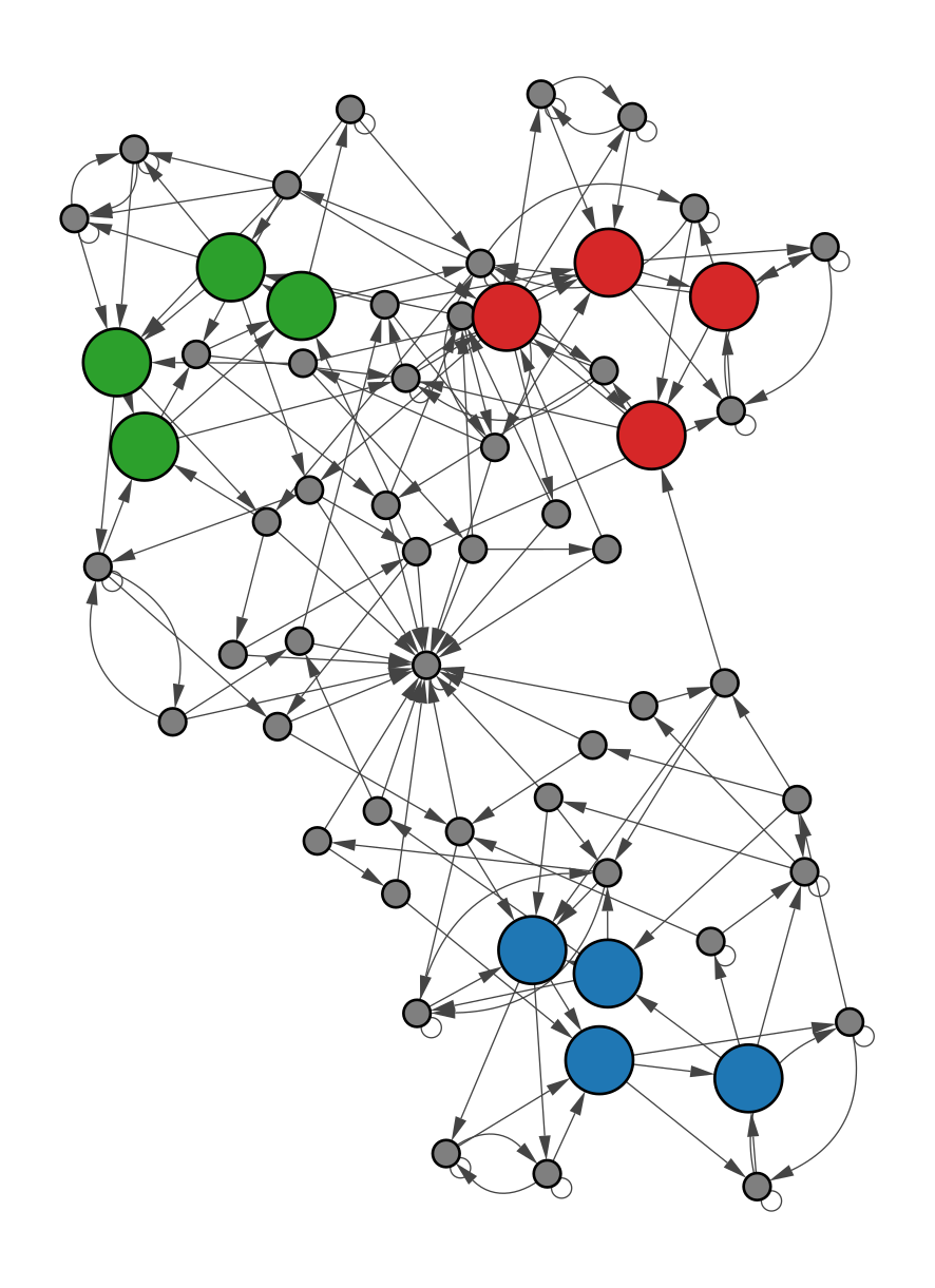
((a))

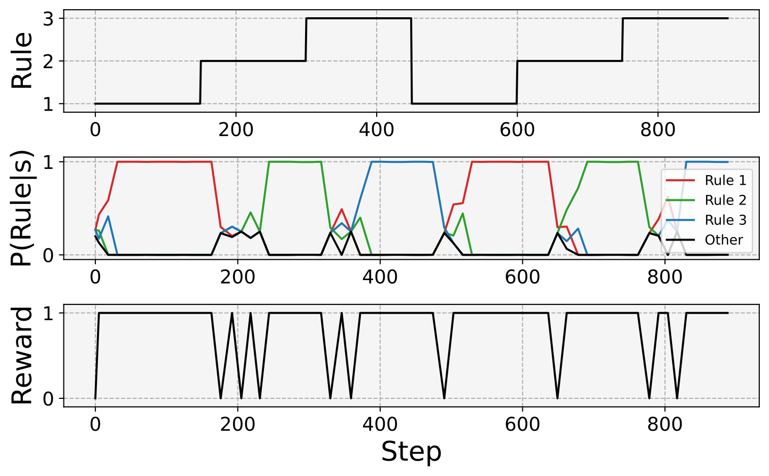
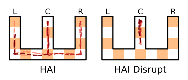
((b))

((c))

Figure 4: Experiment 2: Multiple spatial alternation rules (LCLR, LCRC, and RCRL). (a) Representation of the states used in the CSCG for the three distinct rules. States again map to the conjunction of the visited corridor and the presence of reward. Colors in the graph indicate the rule for which the state is used (red for rule 1, green for rule 2, and blue for rule 3). The gray nodes represent other states, either without reward or in transition between multiple rules (b) Performance during a representative trial of 1000 steps, during which the rule switches randomly, every 150 steps. The top plot shows the rule that is currently in play. The center plot shows the belief over rule, which is computed by first extracting states belonging to a single rule, and then measuring the likelihood of being in one of these states. The bottom plot shows the rewards collected over time. (c) Disruption experiment for rule switching, when communication between the level 1 and level 2 model is suppressed, perseveration behavior is observed. Trajectory order is indicated by the shade where lighter is earlier, noise was added to the trajectory to visualize overlapping visits.

The learned cognitive map of task space is visualized in Figure 4(a). For ease of visualization, we extract the states that are active when the agent has correctly inferred the rule, after a warmup period (15 steps) in each block. Similar to Section 2.2, the states of the task space correspond to the distinct colors, however since the different rules have distinct transition dynamics, these are mapped to unique states. Figure 4(a) uses different colors to visualize the states of the three different rules (red for rule 1, green for rule 2, and blue for rule 3). The smaller dark gray states are states used for transitioning between rules, or encode the corridors where no reward is found. We observe that for each of the individual rules, four states are active. This is an indication of correct learning since four is the optimal number required for each alternation problem.

Then, we evaluate whether the HAI agent is able to infer which rule is currently in place – in order to continue collecting rewards when the rule switches. For this, we test the HAI agent (endowed with a preference to maximize reward) in a task in which the rule switches every 150 steps. Figure 4(c) illustrates the behavior of the agent during a single, representative trial. As shown in the figure, shortly after the rule switches (top panel), the HAI agent is able to correctly update its belief about the current rule in its plan (center panel) and secure rewards (bottom panel). The inference of the rule currently in play follows standard Bayesian approach: when the rule changes, the agent receives unexpected observations (since expected rewards are not delivered) and correctly makes a transition to the subspace of the task rule map that encodes the most likely rule. In the center panel of Figure 4(c), we visualize the belief over each rule as the probability of being in one of the four states used in a particular rule (the rules are color-coded as Figure 4(a)) in or in another phase if the state does not occur in either of the rules (grey line). When the agent has a high probability of a rule, it no longer misses the reward. In some cases, it misses the reward because there is a potential overlap between the two rules. For example, around step 200 it could be either of the rules, as it only picks the right one once, and the wrong one after – which could happen for each corridor in each of the rules. Note that in this architecture, the belief about the currently active rule is implicit in the model, but it could be made explicit by adding a hierarchical layer that maintains a probability distribution over the map or the task one is currently in, as in (Stoianov et al.,, 2022).

2.3.1 Disrupting communication between the two levels yields perseveration behavior

We next test the effect of impairing communication between the two hierarchical levels, as studied in (Den Bakker et al.,, 2022). In this experiment, when a hippocampal SWR is detected, the medial prefrontal cortex (mPFC) is disrupted optogenetically – and this impairment produces perserveration with the current rule.

Here, we model this disruption by completely impairing the communication between the two levels – by preventing level 1 from sending any bottom-up information to level 2 in the HAI agent. Figure 4(c) shows the differences between the physical trajectory of the intact HAI agent (left) and the disrupted HAI agent (right) in which communication between the two levels is impaired. The shade of the trajectory indicates the order of visits (lighter is earlier). The figure shows that while the intact HAI agent follows the correct rule, the disrupted HAI agent perseveres in choosing the center corridor. Interestingly, the agent does check at the unambiguous T-junction to self-localize and ensure that it is still in the correct corridor (which is a feature of the epistemic dynamics of active inference, see Section 4.2), but never selects the next goal in the task rule. This is because, without the bottom-up message from level 1, level 2 is unable to correctly recognize that one phase of the task has been achieved and hence never updates the top-down plan. This result is in line with the findings of (Den Bakker et al.,, 2022), that showed perseveration behavior with impaired hippocampal - prefrontal communication.

3 Discussion

Here, we advanced a novel computational theory of hippocampal (HC) - prefrontal (PFC) interactions during cognitive tasks that require navigating in both physical and task space – such as spatial alternation tasks. Empirical studies of spatial alternation have assessed that they depend on the animal’s spatial memory, which is at least in part maintained by HC-PFC communication (Jones and Wilson,, 2005; Spiers,, 2008; Shin and Jadhav,, 2016; Patai and Spiers,, 2021; Tang et al.,, 2021; Simons and Spiers,, 2003) and that disruption of this communication can impair difficult (outbound) decisions (Jadhav et al.,, 2012) and the ability to switch between multiple rules (Den Bakker et al.,, 2022).

Our computational model is based on – and unites – two established theories. The former is a theory of cognitive map formation, based on a statistical sequence learning algorithm: the clone-structured cognitive graph (CSCG) (George et al.,, 2021). Previous studies assessed that CSCG are computationally effective and have biological validity since they are able to successfully reproduce a number of empirical observations about cognitive map formation in the hippocampus, including for example the emergence of place cell coding and splitter cells (Raju et al.,, 2022; Sun et al.,, 2023). Here we extended this body of work by showing that CSCGs can be used in a hierarchical scheme to learn not just cognitive maps for physical space (putatively linked to hippocampal computations), but also more abstract cognitive maps for task space (putatively linked to prefrontal computations).

Furthermore, we used learned CSCGs as components of a hierarchical generative model for active inference (Parr et al.,, 2022). Active inference is a normative framework to model sentient behavior in terms of free energy minimization and (approximate Bayesian) inference over a generative model, which is gaining popularity in cognitive neuroscience. We have shown that by combining two learned CSCG maps (for physical and task space), it is possible to design an effective hierarchical active inference (HAI) agent able to solve spatial alternation tasks. Interestingly, this scheme affords (hierarchical) planning by only using local computations – that is, top-down and bottom-up message-passing between the two hierarchical levels.

We speculate that the hierarchical message-passing scheme of HAI might help us understand HC - PFC communication during spatial alternation. By simulating the interruption of HC - PFC communication in our model, we were able to correctly reproduce impairments during difficult (outbound) decisions (Jadhav et al.,, 2012) and during rule switching (Den Bakker et al.,, 2022) observed in rodents. Our model suggests that the selective impairment of outbound decisions provoked by hippocampal SWR disruptions (Jadhav et al.,, 2012) is due to the fact that the SWRs convey messages to higher structures, like the PFC, which are used to update a belief about the current stage of the task (specifically, this message is key to propagate the belief about task state at level 2 over time ). This interpretation is in keeping with the idea of (Jadhav et al.,, 2012) that the impairment is at the level of spatial memory, not of hippocampal place coding, but to our knowledge, ours is the first work that provides a mechanistic model of this theoretical proposal.

Furthermore, our model suggests that the perseveration pattern found in (Den Bakker et al.,, 2022) when HC-PFC communication is abolished is due to the inhibition of message passing between the two structures. Indeed, in the second simulation, we prevented level 1 from sending any bottom-up message to level 2 (or equivalently, we prevented level 2 from updating its beliefs based on bottom-up message passing). This assumption is coherent with the finding of (Den Bakker et al.,, 2022) that the only disruption of mPFC that prevents spatial rule switching is one that directly follows hippocampal SWRs – hence highlighting the importance of coherent HC - PFC reactivations to solve spatial alternation tasks. Finally, besides helping understand HC - PFC interactions, our model suggests that looking at the animal’s epistemic behavior during the task (e.g., the selection of actions to self-localize and reduce uncertainty about the current pose) could be important to elucidate its strategy; in particular, whether it aims to maximize reward or also to minimize its uncertainty – as predicted by active inference (Parr et al.,, 2022; Schwartenbeck et al.,, 2019; Rens et al.,, 2023). Future studies might assess whether epistemic imperatives are important drivers of behavior during spatial alternation or similar tasks, especially in conditions of high uncertainty, such as when the animal is randomly placed in a maze (as in our simulations) or when spatial contingencies or task rules change unexpectedly.

The current study has several limitations that will need to be addressed in future studies. First, for efficiency reasons, we learned the CSCGs offline (before embedding them into the HAI), using a simplified procedure: we used predefined trajectories that exhaustively covered the W-maze as inputs for the cognitive map of physical space and 75% correct trajectories as inputs for the cognitive map of task space. In the future, it would be interesting to train CSCG online, similar to (Lazaro-Gredilla et al.,, 2023), by guiding the exploration through active inference dynamics (Friston et al., 2017a, ; Schwartenbeck et al.,, 2019; Parr et al.,, 2022). A second research avenue is to relax the separation of the timescales between the two levels, by selecting their inputs (e.g., level 1 takes all sensory observations as inputs, whereas level 2 only considers reward observations – and in particular, observation 1 in Figure 2(b)). In the future, it would be interesting to explore methods to learn hierarchical models with multiple timescales (Yamashita and Tani,, 2008; Hinton et al.,, 2006) and effective state spaces for navigation and for task rules in self-supervised (and/or reward-guided) ways, as shown in prior work (Stoianov et al.,, 2022, 2018, 2016; Niv,, 2019). A third promising challenge is to avoid having the agent learn from scratch each new maze or rule. Recent work in transfer learning shows that it is possible to reuse existing cognitive maps or latent task representations to learn novel and similar tasks much faster (Stoianov et al.,, 2022; Guntupalli et al.,, 2023; Stoianov et al.,, 2016; Swaminathan et al.,, 2023). Extending our architecture with transfer learning abilities would be important to provide more accurate models of how animals learn cognitive maps, especially given the strong evidence for the reuse of existing neural sequences and cognitive maps in the hippocampus (Liu et al., 2019a, ; Farzanfar et al.,, 2023).

Future studies might consider how to adapt the HAI agent to robot navigation and planning. There is increasing interest in applying active inference to robotic domains, given the appeal of its unified approach to control, state estimation, and world model learning (Lanillos et al.,, 2021; Da Costa et al.,, 2022; Taniguchi et al.,, 2023). Hierarchical active inference is especially appealing, since it affords planning over longer time horizons. For example, one study built a hierarchical model for robot navigation, using multiple layers of recurrent state space models (Çatal et al.,, 2021). Another study realized a hierarchical model for next-frame video prediction, using a subjective timescale for the predictions  (Zakharov et al.,, 2021). In another study (Van de Maele et al.,, 2023), a single layer CSCG was embedded within the active inference framework and was able to support navigation in different mazes. An interesting direction of future work could be adding a (learned) hierarchical layer that maps the high-dimensional observations space to a discrete state space and stack the proposed hierarchical active inference on top with multiple layers of CSCGs. This would potentially afford abstract reasoning and planning for complex tasks, directly from sensory observations such as pixels.

Finally, future studies might consider in more detail the functional role and content of hippocampal reactivations and replay in the hippocampus and other brain structures, such as the prefrontal cortex and the ventral striatum (Wilson and McNaughton,, 1994; Foster,, 2017; Pfeiffer and Foster,, 2013; Liu et al., 2019b, ; Lansink et al.,, 2009; Peyrache et al.,, 2009; Wittkuhn and Schuck,, 2021; Liu et al.,, 2018; Buzsáki,, 2015, 2019; Gupta et al.,, 2010; Nour et al.,, 2021). Previous studies suggested that replay might play different roles, which range from memory functions to planning, compositional computation and the optimization of the brain’s generative models (Stoianov et al.,, 2022; Shin et al.,, 2017; Mattar and Daw,, 2018; Pezzulo et al.,, 2019, 2021; Wittkuhn et al.,, 2021; Kurth-Nelson et al.,, 2023). However, these works have mostly considered hippocampal replay, not coordinated replay in the hippocampus and the prefrontal cortex (and other brain areas). It might be interesting to combine the insights of these studies with the hierarchical architecture of the HAI agent, to test whether (for example) planning and model optimization benefit from the combined replay of multiple brain structures, as opposed to local replay in the hippocampus.

4 Methods

In this paper, we develop a hierarchical planning agent by combining two components: we use clone structured cognitive graphs (CSCG) to learn “cognitive maps” of physical and task space; and hierarchical active inference to form hierarchical plans. In the next sections, we explain the two key components of our approach: CSCG (Section 4.1) and hierarchical active inference (Sec. 4.2). Finally, we explain how we combined these (Section 4.3).

4.1 Clone-structured cognitive graphs (CSCG) for learning cognitive maps of physical and task space

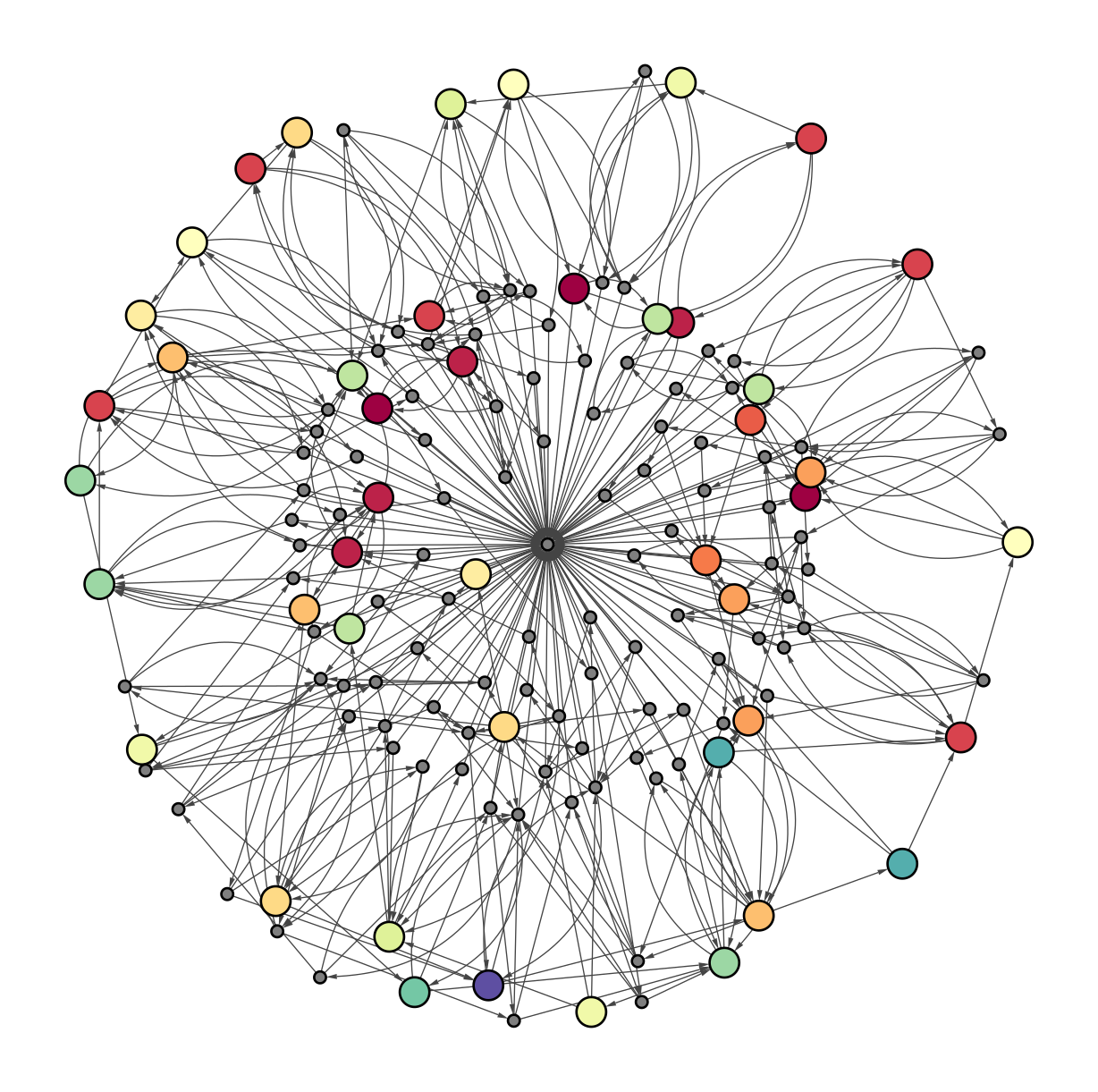
((a))

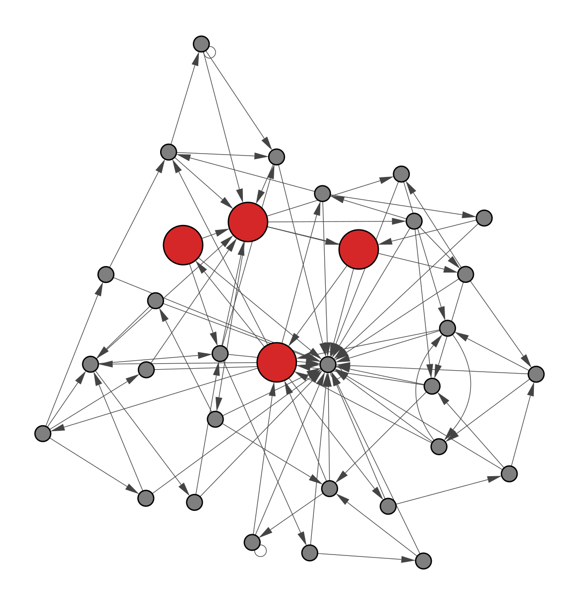
((b))

Figure 5: Learned cognitive graphs. (a) The learned CSCG for the physical space model (level 1). The color in the graph represents distinct observations, only the states that are active when pursuing the spatial alternation rule (LCRC) are colored, the other states are marked in gray. (b) The learned CSCG for the task space model (level 2). The color in the graph indicates the states that were active when pursuing the spatial alternation rule (LCLR).

Clone-structured cognitive graphs (CSCGs) are a probabilistic model for representing sequences of data, e.g. a sequence of action-observation pairs (Gothoskar et al.,, 2019; George et al.,, 2021). They are a special case of Hidden Markov Models (HMM), where each observation maps to a subset of the hidden states: the so-called clones of this observation. While these states have the same observation likelihood, they differ in the implied dynamics encoded in their transition model. Through the sequence of action-observation pairs, specific clones will have a higher likelihood and can therefore disambiguate the aliased observations.

We consider two cognitive maps, that represent the W-maze task at two distinct levels. The first level considers the structure of the environment (i.e. where can the agent walk and where are the walls), and the second level encodes the task rule (i.e. in which order the corridors yields the reward). We learn these two maps in a sequential fashion, using two distinct CSCGs.

We first collect a sequence of data for learning the spatial structure by exploring the maze. We designed the exploration sequence to exhaustively cover the W-maze such that a path from each pose to each possible other pose is present. This sequence was used to learn the parameters of a CSCG for the first (physical) level, using the expectation-maximization mechanism described in (George et al.,, 2021). We initialize the level 1 CSCG with 20 clone states per observation. After learning, the model is pruned using a Viterbi-decoding algorithm as described in (George et al.,, 2021) and mapped to the POMDP of the first level of the hierarchical generative model (as will be explained in Section 4.3) for engaging in active inference. The learned graph is visualized in Figure 5(a). The nodes in the graph correspond to the learned nodes and their colors represent the observations encountered in the states, during the correct execution of the spatial alternation task. The gray nodes represent other states required for transitioning between states or trajectories outside the correct spatial alternation. Note that the graph shown in Figure 2(b) only shows the colored nodes, but not the gray nodes.

We use the learned cognitive map of physical space to learn the cognitive map of task space. We first extract the states that are distinctly representing the end of each corridor (i.e. matching with observation 1 in Figure 2(b)) and use them as the actions for the task level. When an action is selected, this means that the agent is moving toward one of these states, and thus the end of one of the corridors. The observations at this level are the presence of reward (“1” if the agent is following the rule, “0” otherwise), and the reached level 1 state (physical level). To aid the learning process, we guide the agent to follow the rule 75% of the time. We now learn a CSCG with 10 clones per observation using the same expectation-maximization scheme for the single rule scheme, and 32 clones for the scenario with three rules. After learning, the model is pruned using a Viterbi algorithm as described in (George et al.,, 2021) and mapped to the POMDP of the second level of the hierarchical generative model to engage in active inference (see Section 4.3). We visualize the learned cognitive graph in Figure 5(b), where the states used when pursuing the rule are colored in red. It can be observed that the spatial alternation rule is encoded in this graph, using four states, as this is the optimal amount required for the spatial alternation rule (two states for the center, one for the left, and one for the right corridor). Note that the graph shown in Figure 2(b) only shows the colored nodes, but not the gray nodes.

4.2 Hierarchical active inference

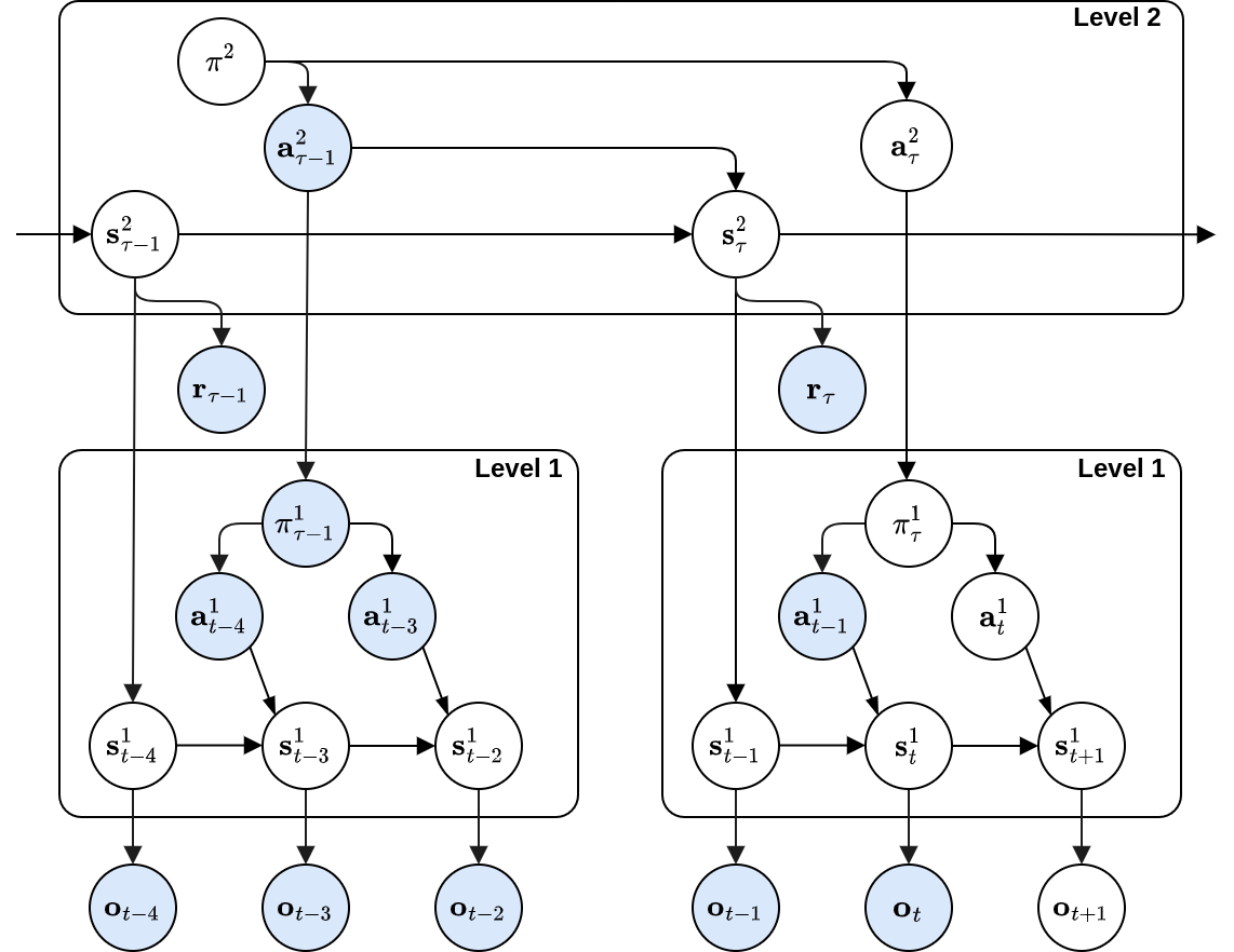
Figure 6: The Hierarchical Generative Model: This generative model consists of two hierarchical levels, where the top level operates at a slower timescale than the lower level. The policy at the highest level sets the actions for the top level, which determines temporal transitions between states at level 2. The level 2 state then generates the presence of reward and the level 1 state. At level 1, the states generate the observations and the policy generates the actions, depending upon the selected level 2 action. Finally, when a policy is pursued, a message is passed to the upper level, transitioning the upper level to the next state. This highlights the different timescales, whereas level 1 operates in the timescale of the agent’s movement, the upper level operates at the timescale of the reached subgoals (visited corridors). Blue circles denote observed variables, while white circles denote unobserved variables.

Active inference is a normative framework to describe cognitive processing and brain dynamics in living organisms (Parr et al.,, 2022). It assumes that action and perception both minimize a common functional: the minimization of variational free energy (which is an upper bound to the organisms’ surprise). Central to active inference is the idea that living organisms are equipped with generative models, capturing the causal relations between observable outcomes, the agent’s actions, and hidden states.

It is important to note the difference between the agent’s generative model and the generative process. The former represents the internal generative model that the agent uses to attribute consequences to its actions, while the latter represents the true process from which outcomes are generated in the world. Crucially, the agent is unable to observe the hidden state of the generative process, as they are separated through a Markov blanket given the observation and action hidden variables. However, the agent is able to perform actions and observe the generated outcomes (Parr et al.,, 2022; Pezzulo et al.,, 2018, 2015).

4.2.1 The hierarchical generative model

We endow the active inference agent with the hierarchical generative model depicted in Figure 6. In this section, we provide a high-level overview of the generative model, whereas in Section 4.3 below we discuss implementation details.

The hierarchical generative model can be split into two distinct levels, each of these levels can be interpreted as an individual partially observable Markov decision process (POMDPs) (Kaelbling et al.,, 1998), operating at different timescales. The highest hierarchical level reasons at a more abstract level, e.g. about which corridor to visit, while the lowest level considers the step-by-step navigation in the environment.

Observations are generated in a top-down fashion according to the hierarchical generative model. Level 2 contains a policy $\pi^{2}$ that generates actions $\mathbf{a}^{2}_{t}$ that follow the rule that is currently in place when the preferred observation is set to find the reward (technically, in active inference, this is done by assuming a strong prior for the reward observation). These actions indicate the location that the agent will then try to reach in the spatial map (level 1). In this way, the level 2-action conditions the level 1 policy $\pi^{1}$. The level 2 state $\mathbf{s}^{2}_{t}$ is a latent representation of the corridor in which the agent is currently located in, and where it comes from (i.e. where the agent is in rule space). This abstraction is enforced by the choice of considering the reachable states to be matched to observation 1 (Figure 2(b)). The agent only considers reward on level 2 and thus generates the presence of reward directly from the level 2 state.

At level 1, the policy $\pi^{1}$ is conditioned by level 2, by setting the preferred state as reaching one of the spatial locations encoded in the cognitive graph. The policy $\pi^{1}$ generates the low-level actions that navigate the agent from one pose (position and orientation, encoded in hidden state $\mathbf{s}_{t}^{1}$) to the next. Finally, the structural observations $\mathbf{o}_{t}$ in the environment are generated from this current pose in the maze. Note that reaching the preferred spatial location requires making multiple transitions at level 1, but level 2 only makes a transition between states when the preference at level 1 is reached (or equivalently when the level 2 action is “performed”). This creates a separation of timescales because multiple transitions at level 1 are nested between two subsequent actions at level 2.

4.2.2 Active inference

As shown in Figure 6, the generative model considered in this paper is a hierarchically stacked (two levels) POMDP. In order to reduce complexity, we first discuss active inference for a single layer POMDP, as depicted in Figure 7. At time step $t$, we have observation $\mathbf{o}_{t}$, action $\mathbf{a}_{t}$ generated from policy $\pi$, and state $\mathbf{s}_{t}$. The generative model is factorized as:

$$P(\mathbf{\tilde{s}},\mathbf{\tilde{a}},\mathbf{\tilde{o}})=P(\mathbf{s}_{0})\prod_{t=1}P(\mathbf{o}_{t}|\mathbf{s}_{t})P(\mathbf{s}_{t}|\mathbf{s}_{t-1},\mathbf{s}_{t-1})P(\mathbf{a}_{t-1}),$$ (1)

where the tilde represents a sequence over time. As computing the posterior distribution over the state is intractable for large state spaces, we resort to variational inference and introduce the approximate posterior $Q(\mathbf{\tilde{s}}|\mathbf{\tilde{o}},\mathbf{\tilde{a}})$, the variational free energy measures the discrepancy between the joint distribution and the approximate posterior:

$$F=\mathbb{E}_{Q(\mathbf{\tilde{s}}|\mathbf{\tilde{o}},\mathbf{\tilde{a}})}[\log Q(\mathbf{\tilde{s}}|\mathbf{\tilde{o}},\mathbf{\tilde{a}})-\log P(\mathbf{\tilde{s}},\mathbf{\tilde{a}},\mathbf{\tilde{o}})]\\$$ (2)

Active inference agents minimize this quantity through learning (by optimizing the model parameters), perception (by estimating the most likely state), and planning (by selecting the policy or action sequence that results in the lowest expected free energy).

The expected free energy $G$ is a quantity that is only used during planning and represents the agent’s variational free energy expected after pursuing a policy $\pi$. It is distinct from the variational free energy, because it requires considering future observations generated from the selected policy, as opposed to the current (and past) observations.

Active inference realizes goal-directed behavior by selecting policies that minimize expected free energy – and that are expected to yield observations that are closer to preferred observations (or prior preferences). This is done by setting the approximate posterior of the policy proportional to this quantity:

$$Q(\pi)=\sigma(\gamma G(\pi)),$$ (3)

where $\sigma$ is the softmax function, and $\gamma$ is a temperature variable. Actions are sampled according to this posterior distribution, where low temperatures yield more deterministic behavior. At a given timestep $\tau$, $G$ is computed for a given policy according to the following quantity as formalized in (Heins et al.,, 2022):

$$G(\pi,\tau)\geq-\underbrace{\mathbb{E}_{Q(\mathbf{o}_{\tau}|\pi)}\big{[}D_{KL}[Q(\mathbf{s}_{\tau}|\mathbf{o}_{\tau},\pi)||Q(\mathbf{s}_{\tau}|\pi)]\big{]}}_{\text{Epistemic value}}-\underbrace{\mathbb{E}_{Q(\mathbf{o}_{\tau}|\pi)}\big{[}\log P(\mathbf{o})\big{]}}_{\text{Pragmatic Value}}$$ (4)

This quantity is decomposed into an epistemic value and a pragmatic value (Friston et al., 2017a, ). The epistemic value computes the expected information gain (Bayesian surprise) between the prior $Q(\mathbf{s}_{\tau}|\pi)$ and posterior $Q(\mathbf{s}_{\tau}|\mathbf{o}_{\tau},\pi)$. Intuitively, this quantity represents how much the agent expects the belief over the state to shift when pursuing this policy. The pragmatic value then measures the expected log probability of observing the preferred observation under the selected policy, intuitively computing how likely it is that this policy will drive the agent to its prior preferences. The full expected free energy for a finite time horizon $T$ is computed as $\sum_{\tau=1}^{T}G(\pi,\tau)$.

4.2.3 Hierarchical active inference

Here, we discuss how the active inference scheme introduced above is extended to realize hierarchical perception and planning, through bottom-up and top-down message passing between the two levels of the hierarchical generative model shown in Figure 6.

During perception, first, the low-level state $\mathbf{s}^{1}$ is inferred given observations $\mathbf{o}_{t}$ and level 1 actions $\mathbf{a}^{1}_{t}$ using the inference mechanism implemented in PyMDP (Heins et al.,, 2022). When the free energy of the lowest level reaches a pre-specified threshold, a message containing the most likely level 1 state $\mathbf{s}^{1}_{t}$ the agent is in is passed to the level above (level 2). This threshold is chosen to be reached when the level 1-preference is reached, and uncertainty is below a fixed level. When level 2 gets this bottom-up message, it queries the environment for the presence of reward and observes $\mathbf{r}_{\tau}$. This conjunction of observations, together with high-level action $\mathbf{a}^{2}$ is used to infer the belief over the level 2 state $Q(\mathbf{s}^{2})$, in the same way as done for level 1.

During planning, i.e. generating a sequence of actions that (should) drive the agent toward its goal, policies are generated in a top-down manner, in the sense that goals set at level 2 determine the prior preference (and then in turn the policy) at level 1. First, the level 2 policy is selected by sampling from the approximate posterior over $\pi^{2}$ proportional to its expected free energy. The action selected at this level then conditions the policy at level 1 $\pi^{1}$, for which in turn the approximate posterior $Q(\pi^{1})$ is computed. The low-level action $\mathbf{a}^{1}_{t}$ is then sampled according to this distribution, similar to the hierarchical generative model described by Friston et al. (Friston et al., 2017b, ).

As depicted in Figure 6, the policy of the lower level sets a limited amount of steps. In particular, when the preference of the lower level is reached, a message is passed to the upper level, transitioning it into the next state. In this way, inferring the policy at the lower level only considers one action of the upper level at a time.

The posterior over the level 2 policy $Q(\pi^{2})$ is first inferred, as it has no dependencies from above. To do this, the expected free energy is computed, for which we look one time step ahead in our implementation as this could predict the next corridor in which the agent encounters reward. We consider Equation 5, for which the observations are now a conjunction of reward $\mathbf{r}_{\tau}$ and level 1-states $\mathbf{s}^{1}$:

$$G^{2}(\pi^{2},\tau)\geq-\mathbb{E}_{Q(\mathbf{r}_{\tau},\mathbf{s}^{1}_{t=\tau}|\pi^{2})}\big{[}D_{KL}[Q(\mathbf{s}^{2}_{\tau}|\mathbf{r}_{\tau},\mathbf{s}^{1}_{t},\pi^{2})||Q(\mathbf{s}^{2}_{\tau}|\pi^{2})]\big{]}-\mathbb{E}_{Q(\mathbf{r}_{\tau},\mathbf{s}^{1}_{t=\tau}|\pi^{2})}\big{[}\log P(\mathbf{r}_{\tau},\mathbf{s}^{1}_{t=\tau})\big{]},$$ (5)

Note that the level 1 state is synchronized with the level 2 state, and only the state observed at this synchronized time is considered, hence we denoted the time index for the level 1 state by $t=\tau$. In practice, we used a temperature ($\gamma$) value of $16.0$ for this level. The action $\mathbf{a}^{2}_{\tau}$ is then sampled according to $Q(\pi^{2})$.

The agent, however, is not able to act upon the physical world yet with this level 2 action. The agent now has to infer the posterior distribution over the policy at level 1 $Q(\pi^{1})$. Because we now want to move towards a specific state, i.e. a disambiguated observation, we set the preference in state space for computing the expected free energy at level 1. In practice, Equation 4, for level 1 then boils down to:

$$G^{1}(\pi^{1},t)\geq-\mathbb{E}_{Q(\mathbf{o}_{t}|\pi^{1})}\big{[}D_{KL}[Q(\mathbf{s}^{1}_{t}|\mathbf{o}_{t},\pi^{1})||Q(\mathbf{s}^{1}_{t}|\pi^{1})]\big{]}-\mathbb{E}_{Q(\mathbf{s}^{1}_{t}|\pi^{1})}\big{[}\log P(\mathbf{s}^{1}_{t})\big{]},$$ (6)

where the first term yields the expected information gain after pursuing policy $\pi^{1}$, and the latter the expected utility. In other words, how close the expected state is from the preferred state, set by the action of the level above. This quantity is then used to approximate the posterior over the policy at level 1 from which action $\mathbf{a}^{1}_{t}$ is sampled. At this level, we set a temperature ($\gamma$) value of $0.5$. Crucially, in order to evaluate $G^{1}$ at planning depth 1, we set the prior preference ($\mathbf{C}$ matrix) as such that the preference for each state is proportional to the distance to the goal, i.e. intuitively this means that the agent can follow a breadcrumb trail towards the goal, given that it properly inferred the current state.

4.3 Casting CSCGs as partially observable Markov decision processes

CSCGs can be used directly to plan (George et al.,, 2021). However, in this work, we use the two learned CSCGs to create a hierarchical generative model for active inference – and then use hierarchical active inference to solve the spatial alternation tasks.

Using the two CSCGs to create a hierarchical generative model for active inference requires mapping them into two partially observable Markov decision processes (POMDPs) (Kaelbling et al.,, 1998), the mathematical framework used in discrete time active inference.

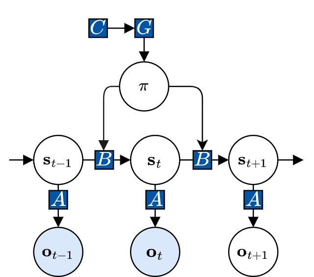
Figure 7: Factor graph of a POMDP: The conditional dependencies in Hidden Markov Models are parameterized by a set of matrices. The $\mathbf{A}$ matrix parameterizes the likelihood model, i.e. how states $\mathbf{s}_{t}$ map to observations $\mathbf{o}_{t}$. The $\mathbf{B}$ matrix parameterizes the transition model, i.e. how state $\mathbf{s}_{t+1}$ changes at each timestep, dependent on policy $\mathbf{\pi}$. The $\mathbf{C}$ vector denotes the preferred observation or state, and directly influences the $\mathbf{G}$ factor on which the policy $\pi$ is conditioned. Blue circles denote that the variable is observed.

Practically, a POMDP is described by a set of four arrays as shown in Figure 7. We describe these arrays using the symbol notation typically adopted in discrete time active inference (Parr et al.,, 2022). The $\mathbf{A}$ matrix encompasses the likelihood model $P(\mathbf{o}|\mathbf{s})$, or how states are mapped to observations. The $\mathbf{B}$ tensor entails the transition model $P(\mathbf{s}_{t+1}|\mathbf{s}_{t},\mathbf{a}_{t})$, or how states change over time, conditioned on the selected action. The $\mathbf{C}$ vector sets the prior over future observations or states, depending on the implementation. This vector is used within active inference to embed the preference or goal state/observation into the agent. Finally, the $\mathbf{D}$ vector describes the initial belief over the state $P(\mathbf{s})$.

As mentioned earlier, clone-structured cognitive graphs are a special case of hidden Markov models and can be therefore easily mapped to POMDPs (which extend HMMs, too). First, we consider the mapping of the likelihood. This $\mathbf{A}$ matrix represents the mapping of observation to state, specifically $\mathbf{A}_{i,j}=P(\mathbf{o}_{i}|\mathbf{s}_{j})$. The matrix can be constructed through the definition of the CSCG, a deterministic mapping of clone state to its observation is set: $P(\mathbf{o}_{i}|\mathbf{s}_{j})=1\forall\mathbf{s}_{j}\in C(\mathbf{o}_{i})$ and $P(\mathbf{o}_{i}|\mathbf{s}_{j})=0\forall\mathbf{s}_{j}\notin C(\mathbf{o}_{i})$, where $C(\mathbf{o}_{i})$ denotes all clone states for observation $\mathbf{o}_{i}$. When constructing the model we only consider states for which the marginalized probability $P(\mathbf{s}_{j})$ surpasses a threshold of $0.0001$. Finally, we add an additional “dummy” state to the additional “dummy” observation, to which unlikely actions are mapped (see below).

To define the transition model, or $\mathbf{B}$ tensor, we use the learned parameters of the model. Through the learning process described in Section 4.1, the CSCG has learned the transition probability $P(\mathbf{s}_{t+1}|\mathbf{s}_{t},\mathbf{a}_{t})$. This is parameterized as a tensor for which $\mathbf{B}_{i,j,k}=P(\mathbf{s}_{i}|\mathbf{s}_{j},\mathbf{a}_{k})$. We construct this tensor with the learned probabilities, for the same states that are considered in the likelihood matrix. Note that for ease of implementation, the active inference routines that we used require that any action could be executed from any state. However, in our task, some actions are not available or highly unlikely in some states (e.g., turning actions in a corridor). To handle this, we created a “dummy state” in the POMDP, which corresponds to observation 20 in Figure 2(b) to which we map the “highly unlikely” actions and to which we assign a large negative value (see below) to ensure that it is never selected during planning. In practice, we set a transition probability of $10^{-12}$ from every state to the dummy state (after which we re-normalize the tensor to sum to one for each action and state). We also set a self-transition of $1$ for the dummy state, therefore ensuring that it is “absorbing”.

Finally, we endow the active inference agent with prior preferences to secure rewards in the spatial alternation tasks in the $\mathbf{C}$ matrix. For ease of implementation, we set these prior preferences manually, rather than extracting them from the learned parameters of the CSCG. For level 2, we set a preference over the conjunction of observations where the reward is $1$ to encourage the agent to follow the learned rule. As described above, when the level 2 action is selected, it sets the $\mathbf{C}$ matrix of level 1 to a large preference for the preferred state and to a value proportional to the distance (in the learned state space of level 1) from said given state to the preferred state (except for the dummy state, for which the $\mathbf{C}$ vector has a fixed value. This is set to the lowest value, making the dummy state the least preferred state).

Finally, the $\mathbf{D}$ matrix is set as a prior over the state. We parameterize this as a uniform distribution over all the states, except for the dummy state. This reflects the fact that in our simulations, the active inference agent is placed in the W-maze with a random pose and has to self-localize.

References

- Basu et al., (2021) Basu, R., Gebauer, R., Herfurth, T., Kolb, S., Golipour, Z., Tchumatchenko, T., and Ito, H. T. (2021). The orbitofrontal cortex maps future navigational goals. Nature, 599(7885):449–452.
- Bellmund et al., (2018) Bellmund, J. L., Gärdenfors, P., Moser, E. I., and Doeller, C. F. (2018). Navigating cognition: Spatial codes for human thinking. Science, 362(6415):eaat6766.
- Benchenane et al., (2011) Benchenane, K., Tiesinga, P. H., and Battaglia, F. P. (2011). Oscillations in the prefrontal cortex: a gateway to memory and attention. Current Opinion in Neurobiology, 21(3):475–485.
- Bogacz, (2017) Bogacz, R. (2017). A tutorial on the free-energy framework for modelling perception and learning. Journal of Mathematical Psychology, 76:198–211.
- Buckley et al., (2017) Buckley, C. L., Kim, C. S., McGregor, S., and Seth, A. K. (2017). The free energy principle for action and perception: A mathematical review. Journal of Mathematical Psychology, 81:55–79.
- Buzsáki, (2015) Buzsáki, G. (2015). Hippocampal sharp wave-ripple: A cognitive biomarker for episodic memory and planning. Hippocampus, 25(10):1073–1188.
- Buzsáki, (2019) Buzsáki, G. (2019). The brain from inside out. Oxford University Press.
- Buzsáki and Moser, (2013) Buzsáki, G. and Moser, E. I. (2013). Memory, navigation and theta rhythm in the hippocampal-entorhinal system. Nature neuroscience, 16(2):130–138.
- Chevalier-Boisvert et al., (2018) Chevalier-Boisvert, M., Willems, L., and Pal, S. (2018). Minimalistic gridworld environment for gymnasium.
- Colgin, (2011) Colgin, L. L. (2011). Oscillations and hippocampal–prefrontal synchrony. Current opinion in neurobiology, 21(3):467–474.
- Da Costa et al., (2022) Da Costa, L., Lanillos, P., Sajid, N., Friston, K., and Khan, S. (2022). How Active Inference Could Help Revolutionise Robotics. Entropy, 24(3):361.
- Den Bakker et al., (2022) Den Bakker, H., Van Dijck, M., Sun, J.-J., and Kloosterman, F. (2022). Sharp-wave ripple associated activity in the medial prefrontal cortex supports spatial rule switching. preprint, Neuroscience.
- Epstein et al., (2017) Epstein, R. A., Patai, E. Z., Julian, J. B., and Spiers, H. J. (2017). The cognitive map in humans: spatial navigation and beyond. Nature neuroscience, 20(11):1504–1513.
- Farzanfar et al., (2023) Farzanfar, D., Spiers, H. J., Moscovitch, M., and Rosenbaum, R. S. (2023). From cognitive maps to spatial schemas. Nature Reviews Neuroscience, 24(2):63–79.
- Foster, (2017) Foster, D. J. (2017). Replay comes of age. Annual review of neuroscience, 40:581–602.
- Friston, (2010) Friston, K. (2010). The free-energy principle: a unified brain theory? Nature Reviews Neuroscience, 11(2):127–138.
- (17) Friston, K., FitzGerald, T., Rigoli, F., Schwartenbeck, P., and Pezzulo, G. (2017a). Active Inference: A Process Theory. Neural Computation, 29(1):1–49.
- (18) Friston, K. J., Rosch, R., Parr, T., Price, C., and Bowman, H. (2017b). Deep temporal models and active inference. Neuroscience & Biobehavioral Reviews, 77:388–402.
- George et al., (2021) George, D., Rikhye, R. V., Gothoskar, N., Guntupalli, J. S., Dedieu, A., and Lázaro-Gredilla, M. (2021). Clone-structured graph representations enable flexible learning and vicarious evaluation of cognitive maps. Nature Communications, 12(1):2392.
- Gothoskar et al., (2019) Gothoskar, N., Guntupalli, J. S., Rikhye, R. V., Lázaro-Gredilla, M., and George, D. (2019). Different clones for different contexts: Hippocampal cognitive maps as higher-order graphs of a cloned hmm. bioRxiv, page 745950.
- Guntupalli et al., (2023) Guntupalli, J. S., Raju, R. V., Kushagra, S., Wendelken, C., Sawyer, D., Deshpande, I., Zhou, G., Lázaro-Gredilla, M., and George, D. (2023). Graph schemas as abstractions for transfer learning, inference, and planning. arXiv preprint arXiv:2302.07350.
- Gupta et al., (2010) Gupta, A. S., Van Der Meer, M. A., Touretzky, D. S., and Redish, A. D. (2010). Hippocampal replay is not a simple function of experience. Neuron, 65(5):695–705.
- Hafting et al., (2005) Hafting, T., Fyhn, M., Molden, S., Moser, M.-B., and Moser, E. I. (2005). Microstructure of a spatial map in the entorhinal cortex. Nature, 436(7052):801–806.
- Heins et al., (2022) Heins, C., Millidge, B., Demekas, D., Klein, B., Friston, K., Couzin, I., and Tschantz, A. (2022). pymdp: A Python library for active inference in discrete state spaces. Publisher: arXiv Version Number: 2.
- Hinton et al., (2006) Hinton, G. E., Osindero, S., and Teh, Y.-W. (2006). A fast learning algorithm for deep belief nets. Neural computation, 18(7):1527–1554.
- Isomura et al., (2023) Isomura, T., Kotani, K., Jimbo, Y., and Friston, K. J. (2023). Experimental validation of the free-energy principle with in vitro neural networks. Nature Communications, 14(1):4547.
- Ito et al., (2015) Ito, H. T., Zhang, S.-J., Witter, M. P., Moser, E. I., and Moser, M.-B. (2015). A prefrontal–thalamo–hippocampal circuit for goal-directed spatial navigation. Nature, 522(7554):50–55.
- Jadhav et al., (2012) Jadhav, S. P., Kemere, C., German, P. W., and Frank, L. M. (2012). Awake Hippocampal Sharp-Wave Ripples Support Spatial Memory. Science, 336(6087):1454–1458.
- Jones and Wilson, (2005) Jones, M. W. and Wilson, M. A. (2005). Theta Rhythms Coordinate Hippocampal–Prefrontal Interactions in a Spatial Memory Task. PLoS Biology, 3(12):e402.
- Kaelbling et al., (1998) Kaelbling, L. P., Littman, M. L., and Cassandra, A. R. (1998). Planning and acting in partially observable stochastic domains. Artificial intelligence, 101(1-2):99–134.
- Khodagholy et al., (2017) Khodagholy, D., Gelinas, J. N., and Buzsáki, G. (2017). Learning-enhanced coupling between ripple oscillations in association cortices and hippocampus. Science, 358(6361):369–372.
- Kurth-Nelson et al., (2023) Kurth-Nelson, Z., Behrens, T., Wayne, G., Miller, K., Luettgau, L., Dolan, R., Liu, Y., and Schwartenbeck, P. (2023). Replay and compositional computation. Neuron, 111(4):454–469.
- Lanillos et al., (2021) Lanillos, P., Meo, C., Pezzato, C., Meera, A. A., Baioumy, M., Ohata, W., Tschantz, A., Millidge, B., Wisse, M., Buckley, C. L., and Tani, J. (2021). Active Inference in Robotics and Artificial Agents: Survey and Challenges. Publisher: arXiv Version Number: 1.
- Lansink et al., (2009) Lansink, C. S., Goltstein, P. M., Lankelma, J. V., McNaughton, B. L., and Pennartz, C. M. (2009). Hippocampus leads ventral striatum in replay of place-reward information. PLoS biology, 7(8):e1000173.
- Lazaro-Gredilla et al., (2023) Lazaro-Gredilla, M., Deshpande, I., Swaminathan, S., Dave, M., and George, D. (2023). Fast exploration and learning of latent graphs with aliased observations. Publisher: arXiv Version Number: 3.
- Liu et al., (2018) Liu, K., Sibille, J., and Dragoi, G. (2018). Generative predictive codes by multiplexed hippocampal neuronal tuplets. Neuron, 99(6):1329–1341.
- (37) Liu, K., Sibille, J., and Dragoi, G. (2019a). Preconfigured patterns are the primary driver of offline multi-neuronal sequence replay. Hippocampus, 29(3):275–283.
- (38) Liu, Y., Dolan, R. J., Kurth-Nelson, Z., and Behrens, T. E. (2019b). Human Replay Spontaneously Reorganizes Experience. Cell, 178(3):640–652.e14.
- Mattar and Daw, (2018) Mattar, M. G. and Daw, N. D. (2018). Prioritized memory access explains planning and hippocampal replay. Nature neuroscience, 21(11):1609–1617.
- Niv, (2019) Niv, Y. (2019). Learning task-state representations. Nature neuroscience, 22(10):1544–1553.
- Nour et al., (2021) Nour, M. M., Liu, Y., Arumuham, A., Kurth-Nelson, Z., and Dolan, R. J. (2021). Impaired neural replay of inferred relationships in schizophrenia. Cell, 184(16):4315–4328.
- O’Keefe and Dostrovsky, (1971) O’Keefe, J. and Dostrovsky, J. (1971). The hippocampus as a spatial map. preliminary evidence from unit activity in the freely-moving rat. Brain Research Volume, 34:171–175.
- O’Keefe and Nadel, (1979) O’Keefe, J. and Nadel, L. (1979). Précis of O’Keefe & Nadel’s The hippocampus as a cognitive map. Behavioral and Brain Sciences, 2(4):487–494.
- Parr et al., (2022) Parr, T., Pezzulo, G., and Friston, K. J. (2022). Active Inference: The Free Energy Principle in Mind, Brain, and Behavior. The MIT Press.
- Patai and Spiers, (2021) Patai, E. Z. and Spiers, H. J. (2021). The Versatile Wayfinder: Prefrontal Contributions to Spatial Navigation. Trends in Cognitive Sciences, 25(6):520–533.
- Peyrache et al., (2009) Peyrache, A., Khamassi, M., Benchenane, K., Wiener, S. I., and Battaglia, F. P. (2009). Replay of rule-learning related neural patterns in the prefrontal cortex during sleep. Nature neuroscience, 12(7):919–926.
- Pezzulo et al., (2019) Pezzulo, G., Donnarumma, F., Maisto, D., and Stoianov, I. (2019). Planning at decision time and in the background during spatial navigation. Current opinion in behavioral sciences, 29:69–76.
- Pezzulo et al., (2015) Pezzulo, G., Rigoli, F., and Friston, K. (2015). Active inference, homeostatic regulation and adaptive behavioural control. Progress in neurobiology, 134:17–35.
- Pezzulo et al., (2018) Pezzulo, G., Rigoli, F., and Friston, K. J. (2018). Hierarchical active inference: a theory of motivated control. Trends in cognitive sciences, 22(4):294–306.
- Pezzulo et al., (2014) Pezzulo, G., Verschure, P. F., Balkenius, C., and Pennartz, C. M. (2014). The principles of goal-directed decision-making: from neural mechanisms to computation and robotics.
- Pezzulo et al., (2021) Pezzulo, G., Zorzi, M., and Corbetta, M. (2021). The secret life of predictive brains: what’s spontaneous activity for? Trends in Cognitive Sciences, 25(9):730–743.
- Pfeiffer and Foster, (2013) Pfeiffer, B. E. and Foster, D. J. (2013). Hippocampal place-cell sequences depict future paths to remembered goals. Nature, 497(7447):74–79.
- Raju et al., (2022) Raju, R. V., Guntupalli, J. S., Zhou, G., Lázaro-Gredilla, M., and George, D. (2022). Space is a latent sequence: Structured sequence learning as a unified theory of representation in the hippocampus. Publisher: arXiv Version Number: 1.
- Rens et al., (2023) Rens, N., Lancia, G. L., Eluchans, M., Schwartenbeck, P., Cunnington, R., and Pezzulo, G. (2023). Evidence for entropy maximisation in human free choice behaviour. Cognition, 232:105328.
- Schuck et al., (2016) Schuck, N., Cai, M., Wilson, R., and Niv, Y. (2016). Human Orbitofrontal Cortex Represents a Cognitive Map of State Space. Neuron, 91(6):1402–1412.
- Schwartenbeck et al., (2019) Schwartenbeck, P., Passecker, J., Hauser, T. U., FitzGerald, T. H., Kronbichler, M., and Friston, K. J. (2019). Computational mechanisms of curiosity and goal-directed exploration. eLife, 8:e41703.
- Shin et al., (2017) Shin, H., Lee, J. K., Kim, J., and Kim, J. (2017). Continual Learning with Deep Generative Replay. arXiv:1705.08690 [cs].
- Shin and Jadhav, (2016) Shin, J. D. and Jadhav, S. P. (2016). Multiple modes of hippocampal–prefrontal interactions in memory-guided behavior. Current Opinion in Neurobiology, 40:161–169.
- Siapas et al., (2005) Siapas, A. G., Lubenov, E. V., and Wilson, M. A. (2005). Prefrontal phase locking to hippocampal theta oscillations. Neuron, 46(1):141–151.
- Simons and Spiers, (2003) Simons, J. S. and Spiers, H. J. (2003). Prefrontal and medial temporal lobe interactions in long-term memory. Nature reviews neuroscience, 4(8):637–648.
- Smith et al., (2022) Smith, R., Friston, K. J., and Whyte, C. J. (2022). A step-by-step tutorial on active inference and its application to empirical data. Journal of Mathematical Psychology, 107:102632.
- Spiers, (2008) Spiers, H. J. (2008). Keeping the goal in mind: Prefrontal contributions to spatial navigation. Neuropsychologia, 46(7):2106–2108.
- Stoianov et al., (2016) Stoianov, I., Genovesio, A., and Pezzulo, G. (2016). Prefrontal goal codes emerge as latent states in probabilistic value learning. Journal of Cognitive Neuroscience, 28(1):140–157.
- Stoianov et al., (2022) Stoianov, I., Maisto, D., and Pezzulo, G. (2022). The hippocampal formation as a hierarchical generative model supporting generative replay and continual learning. Progress in Neurobiology, 217:102329.
- Stoianov et al., (2018) Stoianov, I. P., Pennartz, C. M., Lansink, C. S., and Pezzulo, G. (2018). Model-based spatial navigation in the hippocampus-ventral striatum circuit: A computational analysis. PLoS computational biology, 14(9):e1006316.
- Sun et al., (2023) Sun, W., Winnubst, J., Natrajan, M., Lai, C., Kajikawa, K., Michaelos, M., Gattoni, R., Fitzgerald, J. E., and Spruston, N. (2023). Learning produces a hippocampal cognitive map in the form of an orthogonalized state machine. preprint, Neuroscience.
- Swaminathan et al., (2023) Swaminathan, S., Dedieu, A., Raju, R. V., Shanahan, M., Lazaro-Gredilla, M., and George, D. (2023). Schema-learning and rebinding as mechanisms of in-context learning and emergence. Publisher: arXiv Version Number: 1.
- Tang et al., (2021) Tang, W., Shin, J. D., and Jadhav, S. P. (2021). Multiple time-scales of decision-making in the hippocampus and prefrontal cortex. eLife, 10:e66227.
- Taniguchi et al., (2023) Taniguchi, T., Murata, S., Suzuki, M., Ognibene, D., Lanillos, P., Ugur, E., Jamone, L., Nakamura, T., Ciria, A., Lara, B., and Pezzulo, G. (2023). World models and predictive coding for cognitive and developmental robotics: frontiers and challenges. Advanced Robotics, 37(13):780–806.
- Tolman, (1948) Tolman, E. C. (1948). Cognitive maps in rats and men. Psychological review, 55(4):189.
- Van de Maele et al., (2023) Van de Maele, T., Dhoedt, B., Verbelen, T., and Pezzulo, G. (2023). Integrating cognitive map learning and active inference for planning in ambiguous environments. Publisher: arXiv Version Number: 1.
- Verschure et al., (2014) Verschure, P. F., Pennartz, C. M., and Pezzulo, G. (2014). The why, what, where, when and how of goal-directed choice: neuronal and computational principles. Philosophical Transactions of the Royal Society B: Biological Sciences, 369(1655):20130483.
- Wilson and McNaughton, (1994) Wilson, M. A. and McNaughton, B. L. (1994). Reactivation of Hippocampal Ensemble Memories During Sleep. Science, 265(5172):676–679.
- Wittkuhn et al., (2021) Wittkuhn, L., Chien, S., Hall-McMaster, S., and Schuck, N. W. (2021). Replay in minds and machines. Neuroscience & Biobehavioral Reviews, 129:367–388.
- Wittkuhn and Schuck, (2021) Wittkuhn, L. and Schuck, N. W. (2021). Dynamics of fmri patterns reflect sub-second activation sequences and reveal replay in human visual cortex. Nature communications, 12(1):1795.
- Yamashita and Tani, (2008) Yamashita, Y. and Tani, J. (2008). Emergence of functional hierarchy in a multiple timescale neural network model: a humanoid robot experiment. PLoS computational biology, 4(11):e1000220.
- Zakharov et al., (2021) Zakharov, A., Guo, Q., and Fountas, Z. (2021). Variational Predictive Routing with Nested Subjective Timescales. Publisher: arXiv Version Number: 2.
- Çatal et al., (2021) Çatal, O., Verbelen, T., Van De Maele, T., Dhoedt, B., and Safron, A. (2021). Robot navigation as hierarchical active inference. Neural Networks, 142:192–204.