Refining the properties of the TOI-178 system with
CHEOPS and TESS ^,

Abstract

Context. The TOI-178 system consists of a nearby late K-dwarf transited by six planets in the super-Earth to mini-Neptune regime, with radii ranging from $\sim$1.1 to 2.9 $R_{\oplus}$ and orbital periods between 1.9 and 20.7 days. All planets but the innermost one form a chain of Laplace resonances. Mass estimates derived from a preliminary radial velocity (RV) dataset suggest that the planetary densities do not decrease in a monotonic way with the orbital distance to the star, contrary to what one would expect based on simple formation and evolution models.

Aims. To improve the characterisation of this key system and prepare for future studies (in particular with JWST), we perform a detailed photometric study based on 40 new CHEOPS visits, one new TESS sector, as well as previously published CHEOPS, TESS, and NGTS data.

Methods. First we update the parameters of the host star using the new parallax from Gaia EDR3. We then perform a global analysis of the 100 transits contained in our data to refine the physical and orbital parameters of the six planets and study their transit timing variations (TTVs). We also use our extensive dataset to place constraints on the radii and orbital periods of potential additional transiting planets in the system.

Results. Our analysis significantly refines the transit parameters of the six planets, most notably their radii, for which we now obtain relative precisions $\lesssim$3%, with the exception of the smallest planet $b$ for which the precision is 5.1%. Combined with the RV mass estimates, the measured TTVs allow us to constrain the eccentricities of planets $c$ to $g$, which are found to be all below 0.02, as expected from stability requirements. Taken alone, the TTVs also suggest a higher mass for planet $d$ than the one estimated from the RVs, which had been found to yield a surprisingly low density for this planet. However, the masses derived from the current TTV dataset are very prior-dependent and further observations, over a longer temporal baseline, are needed to deepen our understanding of this iconic planetary system.

1 Introduction

Studying the relation between the internal composition of planets found in multi-planet systems and their architecture (i.e. orbital properties) is crucial to improve our understanding of the formation and evolution of planetary systems. In this context, planetary systems forming chains of three-body Laplace resonances, where each consecutive pair of planets are in (or close to) a mean-motion resonance (MMR), are of particular interest. Indeed, the fine-tuning and fragility of such orbital configurations ensure that no significant scattering or collision event has taken place since the formation of the planets in the protoplanetary disc (e.g. Mills et al., 2016). Hence, these systems are real goldmines for constraining the outcome of protoplanetary discs and provide important anchors for planet formation models.

To date, chains of Laplace resonances have only been observed for a few systems: GJ 876 (Rivera et al., 2010), Kepler-60 (Goździewski et al., 2016), Kepler-80 (MacDonald et al., 2016), Kepler-223 (Mills et al., 2016), TRAPPIST-1 (Gillon et al., 2017; Luger et al., 2017), K2-138 (Christiansen et al., 2018; Lopez et al., 2019), TOI-178 (Leleu et al. 2021a, hereafter L21), and TOI-1136 (Dai et al., 2023). All these systems, except GJ 876, are transiting, which provides an opportunity to constrain the masses and eccentricities of the planets via their transit timing variations (TTVs), which may have detectable amplitudes thanks to the proximity of each pair of planets to a MMR. For stars that are bright enough, it is also possible to obtain radial velocity (RV) measurements, that can provide complementary constraints on the planetary masses and orbital parameters. Out of the transiting systems cited above, only K2-138, TOI-1136, and TOI-178 have published RV measurements so far, the other ones being too faint in the visible ($V$-mag$\gtrsim$14). In this work, we focus on the latter of these three systems.

The nearby ($\sim$63 pc) late K-type star TOI-178 was initially flagged by the Transiting Exoplanet Survey Satellite (TESS, Ricker et al. 2015) as a potential host to three transiting sub-Neptunes with orbital periods of 6.56, 9.96, and 10.35 days, based on data from its Sector 2. The 0.4-day difference in the orbital periods of the two outer planetary candidates led Leleu et al. (2019) to hypothesise that they occupied a horseshoe orbital configuration. Thanks to an intensive photometric follow-up with the CHaracterising ExOPlanets Satellite (CHEOPS, Benz et al. 2021), L21 demonstrated that this was actually not the case, and revealed instead a compact system of at least six transiting planets in the super-Earth to mini-Neptune regime, with radii ranging from $\sim$1.1 to 2.9 $R_{\oplus}$ and orbital periods of 1.91, 3.24, 6.56, 9.96, 15.23, and 20.71 days. The five outer planets form a 2:4:6:9:12 chain of Laplace resonances, while the innermost planet $b$ lies just outside the 3:5 MMR with planet $c$, which could indicate that it was previously part of the chain but was then pulled away, possibly by tidal forces.

Using RV measurements obtained with the Echelle SPectrograph for Rocky Exoplanets and Stable Spectroscopic Observations (ESPRESSO, Pepe et al. 2021) installed at ESO’s Very Large Telescope, L21 were also able to derive preliminary estimates for the masses of the planets, and thus their bulk densities (when combined with the radii inferred from the transit photometry). The planetary densities that they found show important variations from planet to planet, jumping for example from $\sim$1 to 0.2 $\rho_{\oplus}$ between planets $c$ and $d$. By doing a Bayesian internal structure analysis, they showed that the two innermost planets are likely to be mostly rocky, which could indicate that they have lost their primordial gas envelope through atmospheric escape, while all the other planets appear to contain significant amounts of water and/or gas (see also the independent internal structure analysis by Acuña et al. 2022). Interestingly, it seems that the amount of gas in the planets does not vary as a monotonic function of the orbital distance to the star, as opposed to what one would expect from simple formation and evolution models and unlike other known systems in a chain of Laplace resonances. The most notable outlier is planet $d$, which seems to have a larger gas mass than planet $e$ (with a probability of 92%), although the latter is more massive and at a larger distance from the star. This is surprising for two reasons. First, from a formation perspective, one would expect that the mass of the primordial gas envelope is a growing function of the total planetary mass. Second, from an evolution point of view, one would also expect that atmospheric evaporation is more effective for planets that are closer to the star. Based on these considerations, we would thus expect planet $d$ to have a smaller gas mass than planet $e$. Another possible outlier is planet $f$, which appears to be the most massive planet in the system, but may still have less gas than planet $e$ (with a probability of $\sim$60%) despite being located further away from the star.

However, the planetary densities on which these results are based are rather poorly constrained (precision $\gtrsim$30%). In particular, the planetary masses presented by L21 were derived using only 46 RV data points, a very limited dataset for such a complex system. Further RV observations are thus needed to confirm and refine these preliminary mass estimates. Complementary constraints on the masses and eccentricities of the planets could also be obtained by monitoring their TTVs, which are expected to be measurable for all but the innermost planet, with predicted amplitudes ranging from a few minutes for the inner planets to a few tens of minutes for the outer ones (L21). Such transit follow-up observations would also be useful to refine the transit parameters of the planets and their radii. Improving the overall characterisation of the TOI-178 system is essential to optimally prepare the atmospheric follow-up observations that are scheduled on JWST/NIRSpec (PI: M. Hooton) for three of its planets ($b$, $d$, and $g$) and support the interpretation of the resulting transmission spectra.

These considerations motivated the work presented here, which consists in a detailed photometric study of the TOI-178 system, based on 40 new CHEOPS visits, one new TESS sector, as well as previously published data. Our extensive dataset contains 100 transits of the six planets in total, about twice more than the transit dataset presented in L21. The paper is structured as follows. In Sect. 2, we update the properties of the host star using the new parallax from Gaia EDR3. Sect. 3 describes all the observations that we used in our work, with a particular focus on the new data presented in this paper. In Sect. 4, we present our detailed analysis of all these data, including a global transit analysis to refine the system parameters and measure the individual transit timings (Sect. 4.1), as well as a search for possible additional transiting planets in the data and an assessment of their detection limits (Sect. 4.2). In Sect. 5, we present a dynamical analysis of the individual transit timings measured for the five outer planets, before concluding in Sect. 6.

2 Stellar properties

L21 already provided a thorough characterisation of the host star. Table 1 gives the effective temperature ($T_{\mathrm{eff}}$), surface gravity (log $g_{\star}$), metallicity ([Fe/H]), and projected rotational velocity ($v$ sin $i_{\star}$) that they derived from a detailed spectroscopic analysis of the 46 ESPRESSO high-resolution spectra. We refine here the stellar radius of TOI-178 in a similar fashion as in L21, but using updated Gaia EDR3 photometry and parallax values. In brief, we employed a Markov-Chain Monte Carlo (MCMC) modified infrared flux method (IRFM; Blackwell & Shallis 1977; Schanche et al. 2020) to compute the bolometric flux by fitting Gaia (Gaia Collaboration et al., 2021), 2MASS (Skrutskie et al., 2006), and WISE (Wright et al., 2010) broadband photometry with stellar atmospheric models (Castelli & Kurucz, 2003). In this process, the spectroscopic parameters from L21 were used as priors on stellar atmospheric model selection. The bolometric flux was then converted into stellar effective temperature and angular diameter, which was subsequently used to determine the stellar radius ($R_{\star}$) of TOI-178 using the offset-corrected Gaia EDR3 parallax (Lindegren et al., 2021). Via this method, we obtained $R_{\star}$ = $0.662\pm 0.010$ $R_{\odot}$, which is similar to the value reported in L21.

Table 1: Updated properties of the host star TOI-178.

Property (unit)	Value	Source
Astrometric properties
RA (J2000)	00:29:12.49	[1]
Dec (J2000)	$-$30:27:14.86	[1]
$\mathrm{\mu_{RA}}$ (mas $\mathrm{yr}^{-1}$)	$150.032\pm 0.028$	[1]
$\mathrm{\mu_{Dec}}$ (mas $\mathrm{yr}^{-1}$)	$-87.132\pm 0.030$	[1]
Parallax (mas)	$15.900\pm 0.031$	[1]
Distance (pc)	$62.89\pm 0.12$	from parallax
Photometric magnitudes
$G$ (mag)	$11.1575\pm 0.0028$	[1]
$G_{\rm BP}$ (mag)	$11.8398\pm 0.0029$	[1]
$G_{\rm RP}$ (mag)	$10.3602\pm 0.0038$	[1]
$J$ (mag)	$9.372\pm 0.021$	[2]
$H$ (mag)	$8.761\pm 0.023$	[2]
$K$ (mag)	$8.656\pm 0.021$	[2]
$W$1 (mag)	$8.573\pm 0.022$	[3]
$W$2 (mag)	$8.64\pm 0.02$	[3]
Spectroscopic and derived properties
$T_{\mathrm{eff}}$ (K)	$4316\pm 70$	Spectroscopy [4]
log $g_{\star}$ (cgs)	$4.45\pm 0.15$	Spectroscopy [4]
$\mathrm{[Fe/H]}$ (dex)	$-0.23\pm 0.05$	Spectroscopy [4]
$v$ sin $i_{\star}$ (km $\mathrm{s}^{-1}$)	$1.5\pm 0.3$	Spectroscopy [4]
$R_{\star}$ ($R_{\odot}$)	$0.662\pm 0.010$	IRFM [5]
$M_{\star}$ ($M_{\odot}$)	$0.647_{-0.029}^{+0.030}$	Isochrones [5]
$t_{\star}$ (Gyr)	$6.0_{-5.0}^{+6.8}$	Isochrones [5]
$L_{\star}$ ($L_{\odot}$)	$0.136\pm 0.010$	from $R_{\star}$ and $T_{\mathrm{eff}}$ [5]
$\rho_{\star}$ ($\rho_{\odot}$)	$2.23\pm 0.14$	from $R_{\star}$ and $M_{\star}$ [5]

References. [1] Gaia EDR3 (Gaia Collaboration et al., 2021); [2] 2MASS (Skrutskie et al., 2006); [3] WISE (Wright et al., 2010); [4] Leleu et al. (2021a); [5] this work (see Sect. 2).

Taking advantage of the $R_{\star}$ revision, we re-derived the isochronal mass ($M_{\star}$) and age ($t_{\star}$) following the same procedure outlined in L21. We inputted [Fe/H], $T_{\mathrm{eff}}$, and $R_{\star}$ into two different stellar evolutionary models, namely PARSEC v1.2S (Marigo et al., 2017) and CLES (Code Liégeois d’Évolution Stellaire, Scuflaire et al., 2008) to obtain two pairs of mass and age estimates. In particular, the first pair ($M_{\star,1}$, $t_{\star,1}$) was computed by the isochrone placement algorithm (Bonfanti et al., 2015, 2016), which interpolates the provided input values within pre-computed grids of PARSEC isochrones and tracks. The routine convergence was further aided by the $v\sin{i_{\star}}$-based gyrochronological relation (with $v\sin{i_{\star}}$ the projected rotational velocity) implemented within the isochrone placement, as described in Bonfanti et al. (2016). The second pair ($M_{\star,2}$, $t_{\star,2}$), instead, was retrieved by CLES, which generates the best-fit ‘on-the-fly’ stellar track, following the Levenberg-Marquardt minimisation scheme presented in Salmon et al. (2021). After carefully checking the mutual consistency of the two respective pairs of outcomes through the $\chi^{2}$-based criterion broadly discussed in Bonfanti et al. (2021), we finally merged the two results and obtained $M_{\star}=0.647_{-0.029}^{+0.030}\,M_{\odot}$ and $t_{\star}=6.0_{-5.0}^{+6.8}$ Gyr. Those values are similar to those reported in L21. Our revised stellar parameters are presented at the bottom of Table 1.

3 Data

In this section, we describe all the photometric data that we used in our work. Table 2 summarises the number of transits obtained for each planet and facility, with a total of 100 transits observed for the system. This is about twice more than the transit dataset presented in L21.

Table 2: Number of transits observed for each planet and facility.

	Planet
Facility	b	c	d	e	f	g
CHEOPS	19	9	5	4	4	4
TESS	23	14	6	4	4	2
NGTS	1	–	–	–	–	1
Total number of transits	43	23	11	8	8	7

3.1 CHEOPS

We obtained 44 visits (observation runs) of TOI-178 with CHEOPS (Benz et al., 2021) in total, of which only four were presented previously in L21. These observations were acquired between 21 July 2020 and 18 October 2021 as part of the Guaranteed Time Observations (GTO) program and are summarised in Table 5. Since CHEOPS revolves around the Earth on a low-altitude ($\sim$700 km) Sun-synchronous orbit, the data show some interruptions corresponding to occultations of the target by the Earth or passages through the South Atlantic Anomaly (SAA). For our TOI-178 visits, the resulting observing efficiencies (fraction of time used for science observations) vary between 45 and 93% depending on the date of observation. Due to the relative faintness of TOI-178 ($G$-mag=11.15) for CHEOPS, we used the maximum exposure time of 60 seconds for all visits.

As part of our CHEOPS dataset is the near-continuous 11-day observation performed in August 2020, split into two visits for scheduling reasons, that was previously presented in L21. Among the other 42 visits, 23 of them were scheduled to cover transits of the known planets, while the remaining 19 were ‘fillers’, i.e. observations that are carried out when CHEOPS has no time-constrained or higher-priority observations. In the case of TOI-178, the goal of these fillers was to search for other potential transiting planets in the system but they did not reveal any transit-like signal (see Sect. 4.2). Together, the CHEOPS data covered 19, 9, 5, 4, 4, and 4 transits of TOI-178 b, c, d, e, f, and g, respectively.

The raw data of each visit were automatically processed with the CHEOPS Data Reduction Pipeline (DRP version 13.1.0; Hoyer et al. 2020). In short, the DRP calibrates the raw images (event flagging, bias and gain corrections, linearisation, dark current, and flat field corrections), corrects them for environmental effects (cosmic rays, background, and smearing trails from nearby stars), and performs aperture photometry to extract the target’s flux for four different apertures. Using the pycheops package (Maxted et al., 2022) to analyse the different light curves, we found that the best precision is obtained in this case with the default photometric aperture (25 pixels). Owing to the extended and irregular shape of the CHEOPS Point Spread Function (PSF) and the fact that the field rotates around the target along the spacecraft’s nadir-locked orbit (Benz et al., 2021), nearby background stars can introduce time-variable flux contamination in the photometric aperture, in phase with the spacecraft roll angle (see e.g. Lendl et al. 2020; Bonfanti et al. 2021; Maxted et al. 2022). The DRP also provides an estimation of this contamination by using Gaia DR2 catalogue (Gaia Collaboration et al., 2018) and a PSF template to simulate CHEOPS images of the field of view. For our TOI-178 observations, this contamination varies between 0.03 and 0.09% of the target’s flux and is mostly modulated by the rotation around the target of a nearby background star with $G$-mag=13.3 at a projected sky distance of 60.8″. The light curves were corrected for this contamination.

To get an independent photometric extraction, we also reduced the data with PIPE (Brandeker et al. in prep., Morris et al. 2021, Szabó et al. 2021, Deline et al. 2022, Brandeker et al. 2022), a PSF photometry package developed specifically for CHEOPS that has demonstrated an improved precision for faint stars ($G$-mag $\gtrsim$11) such as TOI-178 in a previous work (Morris et al., 2021). PIPE first uses a principal component analysis (PCA) approach to derive a PSF template library from the data series. The first five principal components (PCs) together with a constant background are then used to fit the individual PSFs of each image using a least-squares minimisation and measure the target’s flux. The number of PCs to use is a trade-off between following systematic PSF changes and overfitting the noise. For faint stars such as TOI-178, the mean PSF (first PC) is sufficient for a good extraction, and attempts to model the PSF better with more PCs usually introduce noise in the extracted light curve. Some advantages of using PSF photometry rather than aperture photometry for faint targets are that: (1) the contributions to the signal of each pixel over the PSF are weighted according to noise so that higher S/N photometry can be extracted; (2) cosmic rays and bad pixels (both hot and telegraphic) are easier to filter out or give lower weight in the fitting process; (3) PSF photometry is less sensitive to contamination from nearby background stars; (4) the background is fit simultaneously with the PSF for the same pixels, which can be an advantage if there is some spatial structure.

For each visit, we estimated the photometric precision by computing the median absolute deviation (MAD) of the difference between two consecutive data points (d$f=f_{i+1}-f_{i}$) of the light curve. This metric is robust to outliers and removes correlated signals (e.g. transits). Table 5 gives the MAD that we obtained for both the DRP and PIPE. We found a significant improvement for PIPE, of 18% on average in terms of MAD. We thus decided to use the PIPE light curves in our global analysis.

3.2 TESS

TESS (Ricker et al., 2015) observed TOI-178 for the first time during Cycle 1/Sector 2 of its primary mission (22 August – 20 September 2018). These data, obtained with a two-minute cadence, were previously presented in L21 and we include them in our global analysis. TESS observed again TOI-178 during Cycle 3/Sector 29 of its extended mission, from 26 August to 22 September 2020. The observations were acquired on CCD 3 of camera 2. The data were processed with the TESS Science Processing Operations Center (SPOC) pipeline (Jenkins et al., 2016) at NASA Ames Research Center. We retrieved the 2-minute cadence Presearch Data Conditioning Simple Aperture Photometry (PDCSAP, Stumpe et al. 2012; Smith et al. 2012; Stumpe et al. 2014) from the Mikulski Archive for Space Telescopes (MAST), using the default quality bitmask. Together, the two TESS sectors covered 23, 14, 6, 4, 4, and 2 transits of TOI-178 b, c, d, e, f, and g, respectively.

3.3 NGTS

We also included in our global analysis the light curves obtained with the Next Generation Transit Survey (NGTS, Wheatley et al. 2018) that were previously published in L21: one transit of planet $b$ observed simultaneously with six telescopes on 11 September 2019 and one transit of planet $g$ observed on 12 October 2019 using seven telescopes, thus a total of 13 light curves. We refer the reader to L21 and references therein for more information about these NGTS data and their reduction.

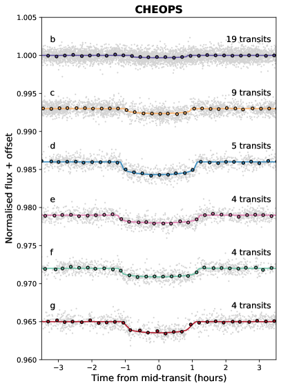
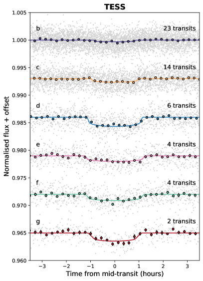
Figure 1: Phase-folded detrended transit photometry of the TOI-178 planets obtained with CHEOPS (left) and TESS (right). For each planet, the photometry was corrected for the measured TTVs and for the transit signals of the other planets. The unbinned data points are shown in grey, while the coloured circles with error bars correspond to 15-min bins. The coloured lines show the best-fit transit models. The number of transits combined in each phase-folded light curve is also indicated in the plot.

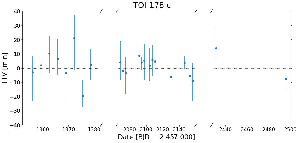
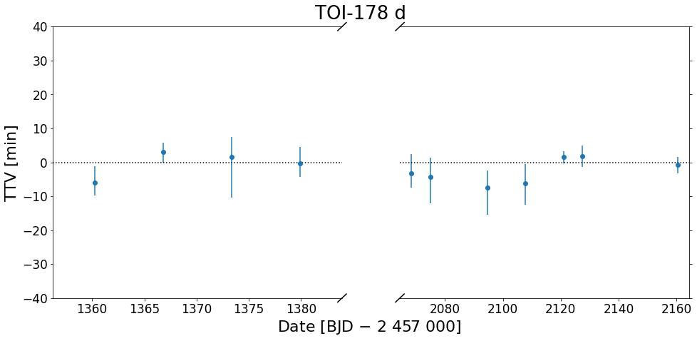
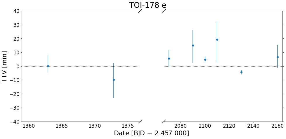
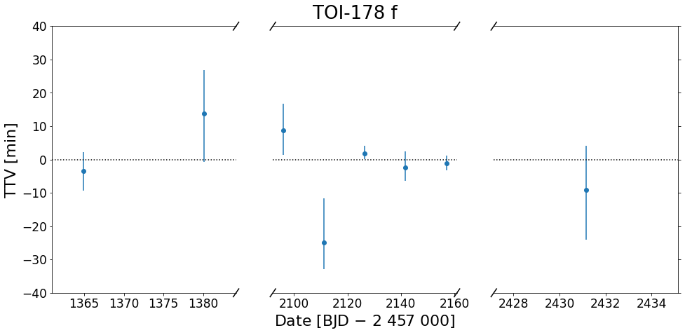
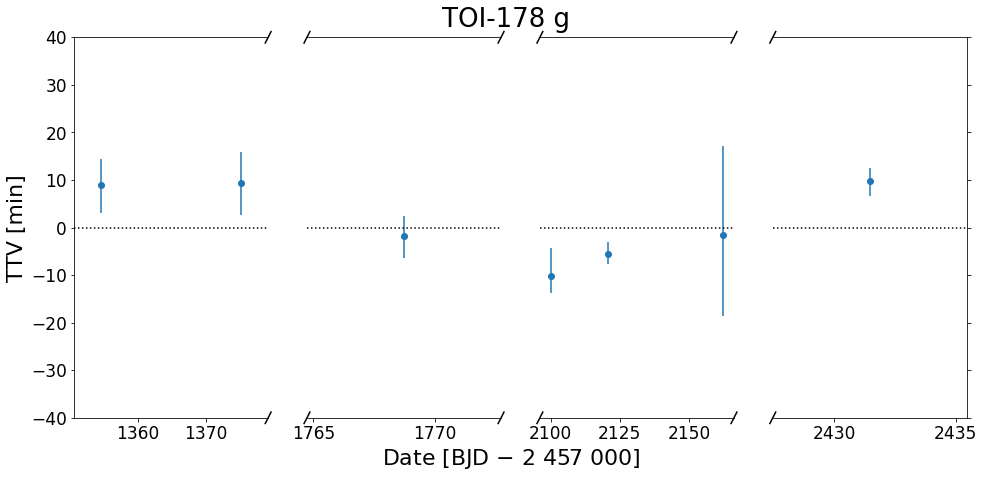
Figure 2: TTVs (in minutes) deduced from our global transit analysis (see Sect. 4.1) for the five outer TOI-178 planets. These TTVs are relative to the updated mean transit ephemerides given in Tables 3 (planets $b$, $c$, and $d$) and 4 (planets $e$, $f$, and $g$). For each planet, we zoomed around the epochs of the observed transits in the $x$-axes for a better visual assessment of the measured TTVs.

4 Data analysis

4.1 Global transit analysis

We performed a joint fit of all the transit photometry described in Sect. 3 using the most recent version of the adaptive MCMC algorithm presented in Gillon et al. (2012, see also Gillon et al. 2014). In order to reduce processing times in this global transit analysis, we only used the portions of the data which contain transits (leaving enough out-of-transit data for proper modelling of the photometric baseline, see below), thus ending up with a total of 96 light curves (summarised in Table LABEL:tab:baselines). These light curves were modelled using the quadratic limb-darkening transit model of Mandel & Agol (2002) multiplied by a photometric baseline model, different for each light curve, aimed at representing the photometric variations caused by other astrophysical, instrumental, or environmental effects. For each light curve, we explored a large range of baseline models, including polynomials, cubic splines, or Gaussian Processes with respect to e.g. time, background, target’s location on the detector, spacecraft roll angle, telescope tube temperature (for CHEOPS), airmass (for NGTS), or combinations of these parameters. Table LABEL:tab:baselines gives the baseline models selected for each light curve based on the Bayesian Information Criterion (BIC, Schwarz 1978). The minimal baseline model is a simple constant to account for any out-of-transit flux offset.

The model parameters sampled by the MCMC were:

• for each planet, the transit depth ($\mathrm{d}F=R_{\mathrm{p}}^{2}/R_{\star}^{2}$ where $R_{\rm{p}}$ is the radius of the planet and $R_{\star}$ is the stellar radius) and the cosine of the orbital inclination (cos $i_{\rm{p}}$);

• the log of the stellar density (log $\rho_{\star}$), the log of the stellar mass (log $M_{\star}$), and the effective temperature ($T_{\rm{eff}}$);

• for the five outer planets, the transit timing variation (TTV, in minutes) of each transit with respect to the transit ephemerides defined by the orbital period ($P$) and the mid-transit time ($T_{0}$) reported in Tables 3 and 4 of L21;

• the log of the orbital period (log $P$) and the mid-transit time ($T_{0}$) of TOI-178 b (we assumed a linear transit ephemeris for this planet as it is not part of the Laplace resonant chain and is thus not expected to show any significant TTVs, see L21);

• for each bandpass (CHEOPS, TESS, and NGTS), the combinations $q_{1}=(u_{1}+u_{2})^{2}$ and $q_{2}=0.5\,u_{1}(u_{1}+u_{2})^{-1}$ of the quadratic limb-darkening coefficients ($u_{1}$ and $u_{2}$), following the triangular sampling scheme advocated by Kipping (2013).

We note that our model thus did not include dynamical interactions between the components of the TOI-178 system; it assumed that there are no mutual interactions between the planets (fixed orbital periods) and then measured TTVs with respect to that Keplerian model. We also assumed circular orbits for all the planets (as justified in Sect. 5, see also L21) and thus set their respective $\sqrt{e}$ cos $\omega$ and $\sqrt{e}$ sin $\omega$ values (with $e$ the eccentricity and $\omega$ the argument of periastron) to zero. Given the large number of light curves, the coefficients of the photometric baseline models were not sampled by the MCMC but determined by a least-squares fit to the residuals at each step of the procedure. This approach allowed us to avoid a dramatic increase in the number of sampled parameters while still fitting the correlated noise simultaneously with the transits (instead of pre-detrending the data), thus ensuring a better propagation of the uncertainties to the derived system parameters of interest (see also similar TTV studies of the TRAPPIST-1 planets by Delrez et al. 2018 and Ducrot et al. 2020).

The prior distributions used in our analysis are summarised in Table 7. We assumed normal priors for $M_{\star}$, $R_{\star}$, and $T_{\rm{eff}}$ based on the values and uncertainties derived in Sect. 2 (Table 1). We also computed normal priors for the quadratic limb-darkening coefficients ($u_{1}$ and $u_{2}$) in each bandpass using the LDCU code (Deline et al., 2022), which builds on the method described by Espinoza & Jordán (2015) to generate limb-darkening coefficients from two libraries of synthetic stellar spectra, ATLAS (Kurucz, 1979) and PHOENIX (Husser et al., 2013), while propagating the uncertainties on the stellar parameters and models.

We first ran a preliminary MCMC chain of 50 000 steps to estimate the two scaling factors, $\beta_{w}$ and $\beta_{r}$ (Table LABEL:tab:baselines), to be applied to the photometric error bars of each light curve to account respectively for over- or under-estimated white noise and the presence of residual correlated (red) noise (for details, see Gillon et al. 2012 and references therein). With the corrected photometric error bars, we then ran two chains of 250 000 steps each (including 25% burn-in) and checked their convergence by using the statistical test of Gelman & Rubin (1992), ensuring that the test values for all sampled parameters were ¡1.01.

Parameter (unit)	Leleu et al. (2021)	This work
TOI-178 b
Transit depth, d$F$ (ppm)	$263_{-30}^{+32}$	$249_{-23}^{+24}$
Transit impact parameter, $b$ ($R_{\star}$)	$0.17_{-0.13}^{+0.19}$	$0.25_{-0.13}^{+0.15}$
Orbital period, $P$ (d)	$1.914558\pm 0.000018$	$1.914554_{-0.000015}^{+0.000018}$
Mid-transit time, $T_{0}$ ($\mathrm{BJD_{TDB}}-2\>450\>000$)	$8\,741.6365_{-0.0030}^{+0.0043}$	$8\,931.1779_{-0.0017}^{+0.0023}$
Transit duration, $W$ (hours)	$1.692_{-0.086}^{+0.056}$	$1.705_{-0.076}^{+0.033}$
Orbital inclination, $i_{\rm{p}}$ (deg)	$88.8_{-1.3}^{+0.8}$	$88.33_{-1.03}^{+0.88}$
Orbital semi-major axis, $a_{\rm{p}}$ (au)	$0.02607\pm 0.00078$	$0.02609_{-0.00034}^{+0.00031}$
Scale parameter, $a_{\mathrm{p}}/R_{\star}$	$8.61_{-0.22}^{+0.21}$	$8.47_{-0.13}^{+0.12}$
Radius, $R_{p}$ (R⊕)	$1.152_{-0.070}^{+0.073}$ (6.3%)	$1.142\pm 0.058$ (5.1%)
Stellar irradiation, $S_{\mathrm{p}}$ ($S_{\oplus}$)	–	$198\pm 14$
TOI-178 c
Transit depth, d$F$ (ppm)	$551_{-59}^{+68}$	$542_{-24}^{+29}$
Transit impact parameter, $b$ ($R_{\star}$)	$0.34_{-0.23}^{+0.30}$	$0.24\pm 0.14$
Orbital period, $P$ (d)	$3.238450_{-0.000019}^{+0.000020}$	$3.238449\pm 0.000011$
Mid-transit time, $T_{0}$ ($\mathrm{BJD_{TDB}}-2\>450\>000$)	$8\,741.4783_{-0.0029}^{+0.0034}$	$8\,926.0680\pm 0.0011$
Transit duration, $W$ (hours)	$1.95_{-0.25}^{+0.15}$	$2.045_{-0.083}^{+0.047}$
Orbital inclination, $i_{\rm{p}}$ (deg)	$88.4_{-1.6}^{+1.1}$	$88.86_{-0.70}^{+0.69}$
Orbital semi-major axis, $a_{\rm{p}}$ (au)	$0.0370\pm 0.0011$	$0.03703_{-0.00048}^{+0.00044}$
Scale parameter, $a_{\mathrm{p}}/R_{\star}$	$12.23_{-0.31}^{+0.29}$	$12.03_{-0.19}^{+0.18}$
Radius, $R_{p}$ (R⊕)	$1.669_{-0.099}^{+0.114}$ (6.8%)	$1.685_{-0.051}^{+0.052}$ (3.1%)
Stellar irradiation, $S_{\mathrm{p}}$ ($S_{\oplus}$)	–	$98.3\pm 7.2$
Orbital eccentricity (TTVs), $e_{\rm{p}}$	–	$0.0073_{-0.0051}^{+0.0083}$
TOI-178 d
Transit depth, d$F$ (ppm)	$1313_{-65}^{+64}$	$1414_{-51}^{+50}$
Transit impact parameter, $b$ ($R_{\star}$)	$0.485_{-0.060}^{+0.051}$	$0.530_{-0.035}^{+0.032}$
Orbital period, $P$ (d)	$6.557700\pm 0.000016$	$6.557721\pm 0.000013$
Mid-transit time, $T_{0}$ ($\mathrm{BJD_{TDB}}-2\>450\>000$)	$8\,747.14623_{-0.00095}^{+0.00087}$	$8\,760.26373\pm 0.00074$
Transit duration, $W$ (hours)	$2.346_{-0.046}^{+0.047}$	$2.323_{-0.034}^{+0.041}$
Orbital inclination, $i_{\rm{p}}$ (deg)	$88.58_{-0.18}^{+0.20}$	$88.42_{-0.11}^{+0.12}$
Orbital semi-major axis, $a_{\rm{p}}$ (au)	$0.0592\pm 0.0018$	$0.05927_{-0.00077}^{+0.00070}$
Scale parameter, $a_{\mathrm{p}}/R_{\star}$	$19.57_{-0.49}^{+0.47}$	$19.25_{-0.30}^{+0.28}$
Radius, $R_{p}$ (R⊕)	$2.572_{-0.078}^{+0.075}$ (3.0%)	$2.717_{-0.061}^{+0.066}$ (2.4%)
Stellar irradiation, $S_{\mathrm{p}}$ ($S_{\oplus}$)	–	$38.4\pm 2.8$
Orbital eccentricity (TTVs), $e_{\rm{p}}$	–	$0.010_{-0.007}^{+0.011}$

Table 3: Properties of the TOI-178 b, c, and d planets based on our global transit analysis (see Sect. 4.1). For planets $c$ and $d$, we also give the eccentricities derived from our TTV analysis (see Sect. 5). For each parameter, we indicate the median of the posterior distribution, along with the 1-$\sigma$ credible intervals. For the planetary radii, we also give the relative uncertainties in brackets.

Parameter (unit)	Leleu et al. (2021)	This work
TOI-178 e
Transit depth, d$F$ (ppm)	$968_{-71}^{+69}$	$917_{-36}^{+33}$
Transit impact parameter, $b$ ($R_{\star}$)	$0.583_{-0.066}^{+0.046}$	$0.595_{-0.025}^{+0.024}$
Orbital period, $P$ (d)	$9.961881\pm 0.000042$	$9.961815\pm 0.000090$
Mid-transit time, $T_{0}$ ($\mathrm{BJD_{TDB}}-2\>450\>000$)	$8\,751.4658_{-0.0019}^{+0.0016}$	$8\,761.4267\pm 0.0032$
Transit duration, $W$ (hours)	$2.501_{-0.077}^{+0.106}$	$2.517_{-0.041}^{+0.045}$
Orbital inclination, $i_{\rm{p}}$ (deg)	$88.71_{-0.13}^{+0.16}$	$88.662_{-0.071}^{+0.066}$
Orbital semi-major axis, $a_{\rm{p}}$ (au)	$0.07833_{-0.00103}^{+0.00093}$	$0.02609_{-0.00034}^{+0.00031}$
Scale parameter, $a_{\mathrm{p}}/R_{\star}$	$25.87_{-0.65}^{+0.62}$	$25.44_{-0.40}^{+0.37}$
Radius, $R_{p}$ (R⊕)	$2.207_{-0.090}^{+0.088}$ (4.1%)	$2.189_{-0.058}^{+0.053}$ (2.6%)
Stellar irradiation, $S_{\mathrm{p}}$ ($S_{\oplus}$)	–	$22.0\pm 1.6$
Orbital eccentricity (TTVs), $e_{\rm{p}}$	–	$0.0080_{-0.0057}^{+0.0100}$
TOI-178 f
Transit depth, d$F$ (ppm)	$1037_{-90}^{+94}$	$1154_{-53}^{+42}$
Transit impact parameter, $b$ ($R_{\star}$)	$0.765_{-0.031}^{+0.027}$	$0.753_{-0.020}^{+0.015}$
Orbital period, $P$ (d)	$15.231915_{-0.000095}^{+0.000105}$	$15.231951\pm 0.000095$
Mid-transit time, $T_{0}$ ($\mathrm{BJD_{TDB}}-2\>450\>000$)	$8\,745.7178_{-0.0027}^{+0.0023}$	$8\,898.0349\pm 0.0017$
Transit duration, $W$ (hours)	$2.348_{-0.087}^{+0.097}$	$2.446_{-0.043}^{+0.052}$
Orbital inclination, $i_{\rm{p}}$ (deg)	$88.723_{-0.069}^{+0.071}$	$88.723_{-0.044}^{+0.047}$
Orbital semi-major axis, $a_{\rm{p}}$ (au)	$0.1039\pm 0.0031$	$0.1040_{-0.0014}^{+0.0012}$
Scale parameter, $a_{\mathrm{p}}/R_{\star}$	$34.33_{-0.87}^{+0.82}$	$33.76_{-0.53}^{+0.49}$
Radius, $R_{p}$ (R⊕)	$2.287_{-0.110}^{+0.108}$ (4.8%)	$2.455_{-0.073}^{+0.061}$ (3.0%)
Stellar irradiation, $S_{\mathrm{p}}$ ($S_{\oplus}$)	–	$12.47\pm 0.91$
Orbital eccentricity (TTVs), $e_{\rm{p}}$	–	$0.0105_{-0.0061}^{+0.0071}$
TOI-178 g
Transit depth, d$F$ (ppm)	$1633_{-139}^{+157}$	$1620_{-62}^{+54}$
Transit impact parameter, $b$ ($R_{\star}$)	$0.866_{-0.019}^{+0.017}$	$0.863_{-0.0105}^{+0.0097}$
Orbital period, $P$ (d)	$20.70950_{-0.00011}^{+0.00014}$	$20.70991\pm 0.00015$
Mid-transit time, $T_{0}$ ($\mathrm{BJD_{TDB}}-2\>450\>000$)	$8\,748.0302_{-0.0017}^{+0.0023}$	$8\,893.0016\pm 0.0026$
Transit duration, $W$ (hours)	$2.167_{-0.082}^{+0.090}$	$2.218_{-0.058}^{+0.061}$
Orbital inclination, $i_{\rm{p}}$ (deg)	$88.823_{-0.047}^{+0.045}$	$88.806_{-0.024}^{+0.023}$
Orbital semi-major axis, $a_{\rm{p}}$ (au)	$0.1275_{-0.0039}^{+0.0038}$	$0.1276_{-0.0017}^{+0.0015}$
Scale parameter, $a_{\mathrm{p}}/R_{\star}$	$42.13_{-1.06}^{+1.01}$	$41.43_{-0.64}^{+0.61}$
Radius, $R_{p}$ (R⊕)	$2.87_{-0.13}^{+0.14}$ (4.9%)	$2.908_{-0.070}^{+0.068}$ (2.4%)
Stellar irradiation, $S_{\mathrm{p}}$ ($S_{\oplus}$)	–	$8.28_{-0.61}^{+0.60}$
Orbital eccentricity (TTVs), $e_{\rm{p}}$	–	$0.0056_{-0.0039}^{+0.0058}$

Table 4: Properties of the TOI-178 e, f, and g planets based on our global transit analysis (see Sect. 4.1). We also give the eccentricities derived from our TTV analysis (see Sect. 5). For each parameter, we indicate the median of the posterior distribution, along with the 1-$\sigma$ credible intervals. For the planetary radii, we also give the relative uncertainties in brackets.

Fig. 1 shows for each planet the phase-folded (TTV-corrected) detrended transit photometry from CHEOPS (left) and TESS (right), with the corresponding best-fit transit models. The medians and 1-$\sigma$ credible intervals of the posterior distributions obtained for the system parameters are given in Tables 3 (planets $b$, $c$, and $d$) and 4 (planets $e$, $f$, and $g$). The transit parameters of the six planets are significantly refined compared to L21, most notably their radii, for which we now obtain a relative precision $\lesssim$3% for all planets, except the smallest planet $b$ for which the precision is 5.1%. Table LABEL:tab:timings presents the individual transit timings that we obtained for the five outer planets. For each of these planets, we performed a linear fit of these transit timings as a function of their epochs to derive updated mean transit ephemerides, which are also given in Tables 3 and 4. The reduced $\chi^{2}$ values of these linear fits are 0.8, 0.9, 2.9, 1.4, and 4.3 for TOI-178 c, d, e, f, and g, respectively. The TTVs with respect to the updated ephemerides are given in Table LABEL:tab:timings and shown in Fig. 2. Only the latest transit of TOI-178 g observed with CHEOPS shows a TTV different from zero at the $\sim$3-$\sigma$ level. A detailed dynamical analysis of the measured transit timings will be presented in Sect. 5.

4.2 Search for additional transiting planets and detection limits

In this section, we first aim to use our large photometric dataset to search for additional transiting planets in the system. We then perform transit injection-and-recovery tests to assess the detection limits of the data and thus place constraints on the radii and orbital periods of potential additional transiting planets in the system.

4.2.1 Search for additional transiting planets

We first searched the TESS data for additional transit signals using the SHERLOCK pipeline presented in Pozuelos et al. (2020, 2023). SHERLOCK downloads the PDCSAP light curve from MAST and, using the Wōtan package (Hippke et al., 2019), applies a biweight sliding filter with varying window sizes to detrend the data. The motivation behind this multi-detrend approach is related to the risk of removing transit signals when detrending the light curve, especially short and shallow ones. Each detrended light curve and the original PDCSAP light curve are then searched for transit signals using the transit least squares (TLS) algorithm (Hippke & Heller, 2019). The transit search is carried out in a loop: once a signal is found, it is stored and masked, and then the search keeps running until no more signals above a user-defined signal detection efficiency (SDE, Hippke & Heller 2019) threshold are found in the dataset. Each of these search-find-mask iterations is called a ‘run’. Here, we analysed the 2 TESS sectors simultaneously and tested 10 different window sizes between 0.2 and 1.2 days for the detrending. We searched the PDCSAP and the 10 detrended light curves for periodic signals with orbital periods ranging from 0.5 to 60 days. For each run, we selected the signal which was found in the greatest number of light curves among these 11 light curves, and with the highest SDE. We recovered the 6 known planets in the first 6 runs in the following order: first TOI-178 d, then TOI-178 c, TOI-178 e, TOI-178 f, TOI-178 b, and finally TOI-178 g. In the subsequent runs, we did not find any other promising signal with a SDE$\geq$5 that could hint at the presence of extra transiting planets in the system.

We then ran SHERLOCK on the CHEOPS data following the same procedure. For this purpose, we pre-detrended the CHEOPS photometry using a cubic spline against the spacecraft roll angle to remove most instrumental noise (e.g. Maxted et al. 2022). We performed a transit search on this light curve as well as 10 further-detrended light curves, each obtained by applying a different biweight time-windowed sliding filter to the first light curve. As with the TESS data, we tested 10 window sizes between 0.2 and 1.2 days. We recovered again the 6 known planets in the first 6 runs: first TOI-178 d, then TOI-178 g, TOI-178 e, TOI-178 f, TOI-178 c, and finally TOI-178 b. Unfortunately, the subsequent runs did not reveal any other promising transit signal.

4.2.2 Detection limits

To assess the detection limits of the data, we performed transit injection-and-recovery tests using the MATRIX ToolKit (Dévora-Pajares & Pozuelos 2022, see also Pozuelos et al. 2020, 2023). We analysed the TESS and CHEOPS data separately, using the same input light curves as for our SHERLOCK transit searches for consistency. For both datasets, we explored planetary radii $R_{\mathrm{p}}$ between 0.5 and 3.5 $R_{\oplus}$ with steps of 0.2 $R_{\oplus}$ and orbital periods $P$ between 1 and 30 days with steps of 1 day. For each $R_{\mathrm{p}}-P$ combination, we injected synthetic transits at 12 random phases (i.e. 12 different values for $T_{0}$), thus giving a total of 5760 scenarios for each dataset. For simplicity, we assumed the impact parameters and eccentricities of the injected planets were zero. For computational cost reasons, only one detrending can be applied to the resulting light curves before trying to recover the injected transits. We chose here to use a biweight filter with a window size of 0.6 day for TESS and 0.8 day for CHEOPS. These window sizes were found to give the best results for the known planets during the SHERLOCK searches described above. We also masked the transits of the 6 known planets. During the transit recovery attempts, we considered a synthetic planet to be properly recovered when its epoch was found with 1 hour accuracy and the recovered period was within 5% of the injected period. Finally, it is worth noting that since we injected the synthetic signals into the PDCSAP light curves for TESS and the roll-angle-decorrelated light curves for CHEOPS, our results do not take into account the possible impact of these systematics corrections on the injected transits. The derived detection limits (discussed below) should therefore be considered rather optimistic (see, e.g., Pozuelos et al. 2020, Eisner et al. 2020).

Fig. 3 shows the two detectability maps in the $R_{\mathrm{p}}-P$ parameter space that we obtained for the TESS (upper panel) and CHEOPS (lower panel) data based on these transit injection-and-recovery tests. We first note that our goal here is not to compare the performances of TESS and CHEOPS. While CHEOPS’s larger primary aperture size and smaller pixel scale make it a higher-precision instrument relative to TESS, the detectability of a transiting planet with a given $R_{\mathrm{p}}$, $P$ and $T_{0}$ will also strongly depend on the number of in-transit data points. In this context, it should be noted that the temporal coverage of the two datasets considered here is very different: the TESS data consist of two sets of nearly-continuous 28-day observations performed in 2018 and 2020, while the CHEOPS data include a nearly-continuous 11-day observation as well as targeted transit windows of the known planets and short observations at random times (fillers, see Sect. 3.1) performed in 2020 and 2021. The CHEOPS data also have a varying observing efficiency depending on the date of observation (see Sect. 3.1). The difference in the number of in-transit data points between the TESS and CHEOPS datasets can thus be very variable depending on the considered scenario. These considerations show that it is necessary to work on a case-by-case basis (i.e. for each $R_{\mathrm{p}}-P-T_{0}$ scenario) if we want to compare the performances of both instruments (see Oddo et al. 2023 for a detailed discussion on this subject). This is not our goal here, which is rather to get a global picture of the overall detection potential of both datasets in the $R_{\mathrm{p}}-P$ parameter space. In this regard, Fig. 3 shows that additional transiting planets in the system with radii ¿1.75 $R_{\oplus}$ and orbital periods ¡12 days can be reasonably ruled out, as they should have been easily detected (recovery rates $\gtrsim$70% in the TESS data and $\gtrsim$50% in the CHEOPS data). The same planetary sizes but with orbital periods between 12 and 24 days have recovery rates ranging from $\sim$70 to 20%. Planets of any size with orbital periods ¿24 days have recovery rates ¡20%. Planets with sizes between 1.5 and 1.75 $R_{\oplus}$ have recovery rates $\gtrsim$50% for orbital periods ¡9 days, while smaller planets with sizes between 1.0 and 1.5 $R_{\oplus}$ only have such reasonably good recovery rates for short orbital periods ¡3 days. Planets smaller than 1 $R_{\oplus}$ would remain undetected in the current dataset, except maybe for short orbital periods ¡3 days (recovery rate $\sim$12% in the CHEOPS data, so this would be challenging).

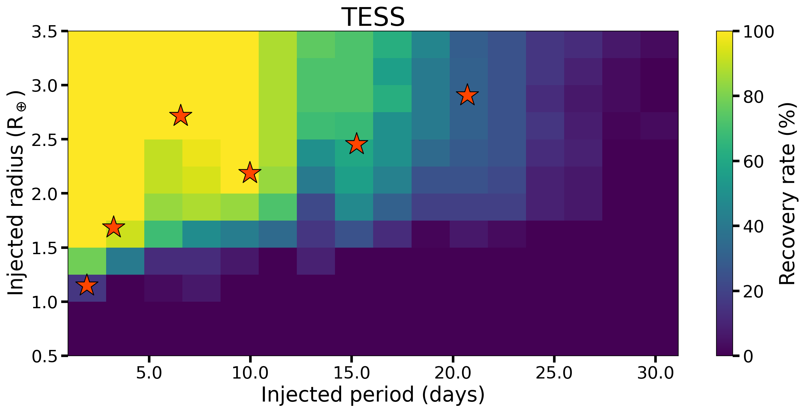
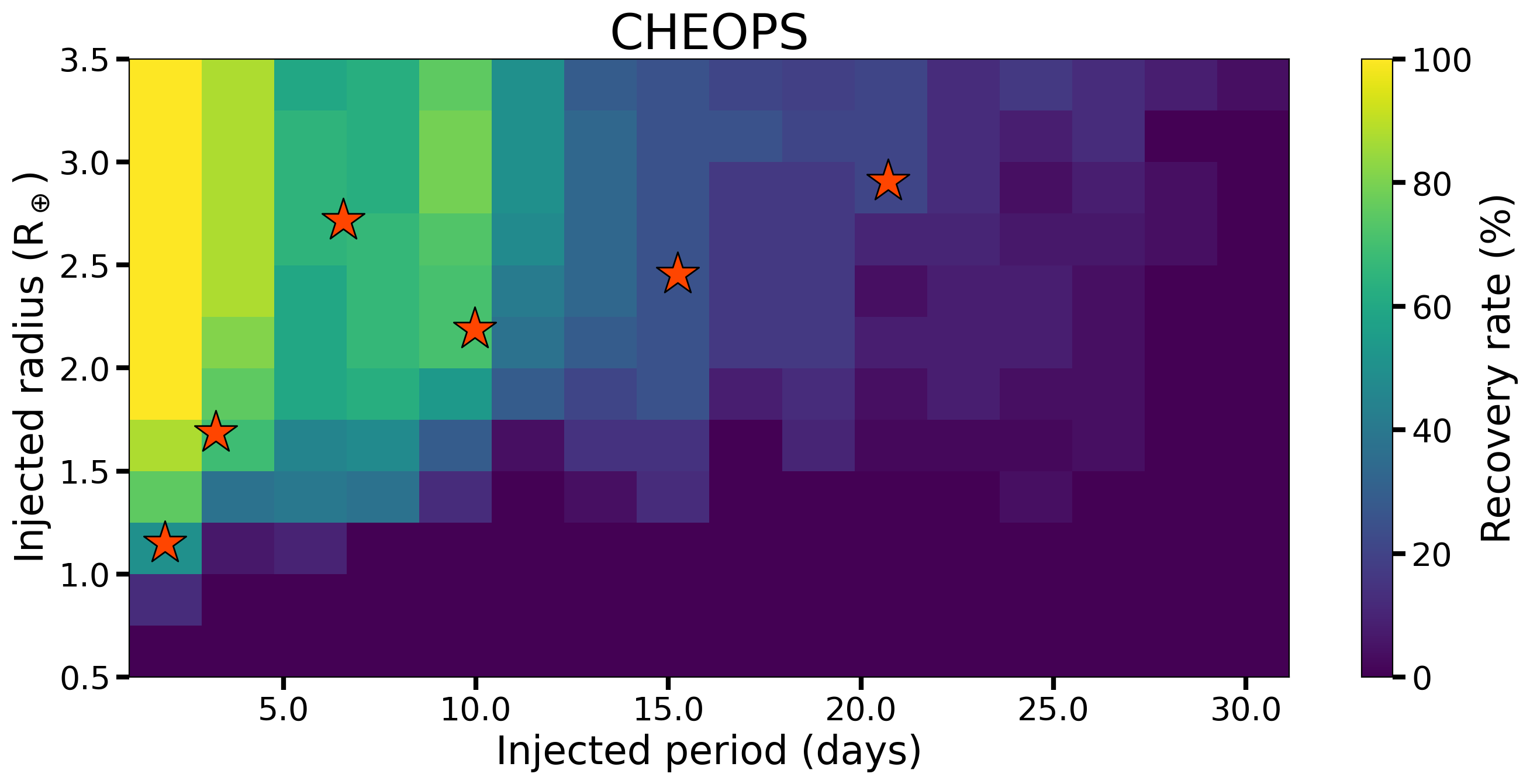
Figure 3: Results of the transit injection-and-recovery tests performed on the TESS (upper panel) and CHEOPS (lower panel) data to assess the detectability of potential additional transiting planets in the TOI-178 system. For both panels, the red stars show the locations of the 6 known planets in the system.

5 Dynamical analysis of the transit timings

All consecutive pairs of planets in the system but the innermost one are close to a first-order MMR where $P_{\mathrm{out}}/P_{\mathrm{in}}\approx(k+1)/k$ with $k$ an integer. As none of the pairs are formally inside the 2-planet MMR, we expect TTVs over the super-period (Lithwick et al., 2012):

$$P_{\mathrm{c,d}}\equiv\frac{1}{|(k+1)/P_{\mathrm{d}}-k/P_{\mathrm{c}}|}\,$$ (1)

for planets $c$ and $d$ as an example, and similarly for the other near-resonant pairs. For TOI-178, the super-period is almost the same for all the near-resonant pairs of planets, with $P_{\mathrm{c,d}}\approx P_{\mathrm{d,e}}\approx P_{\mathrm{e,f}}\approx P_{\mathrm{f,g}}\approx 260$ days. As a result, a Laplace relation links the successive triplets of planets, leading to a slow evolution of the Laplace angles (see L21):

$$\psi_{1} =1\lambda_{\mathrm{c}}-4\lambda_{\mathrm{d}}+3\lambda_{\mathrm{e}}\,,$$ (2)

$$\psi_{2} =2\lambda_{\mathrm{d}}-5\lambda_{\mathrm{e}}+3\lambda_{\mathrm{f}}\,,$$

$$\psi_{3} =1\lambda_{\mathrm{e}}-3\lambda_{\mathrm{f}}+2\lambda_{\mathrm{g}}$$

where $\lambda_{\mathrm{i}}$ is the mean longitude of planet $i$. The evolution of these angles can also produce TTVs on much longer timescales, although according to the mass estimates obtained using radial velocities (see L21), these effects should only start to show with at least 4 years of baseline. Finally, the relative proximity of the planets can also generate a high-frequency chopping signal (Deck & Agol, 2015).

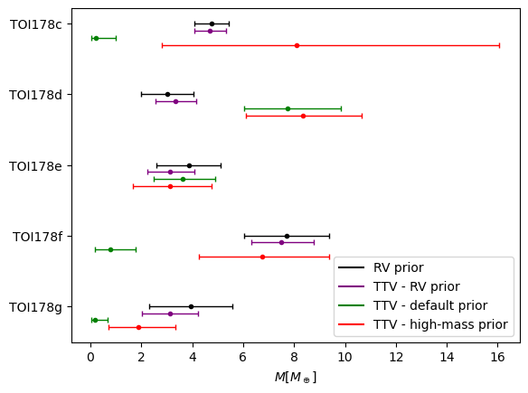
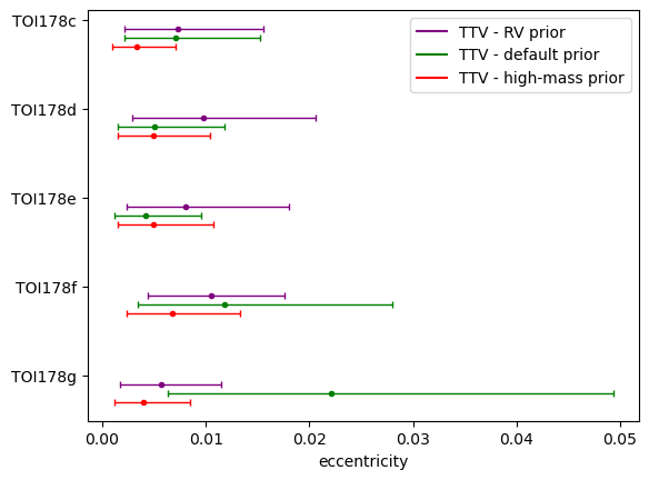
Figure 4: Mass (upper panel) and eccentricity (lower panel) posteriors derived from our dynamical analysis of the TTVs. The corresponding values are given in Table 9. In the upper panel, the radial velocity prior based on the RV measurements presented in L21 is shown in black, with $1\sigma$ error bars. The coloured error bars show the median and .16-.84 quantiles confidence level of the mass posteriors obtained from our TTV fit using three different sets of priors.

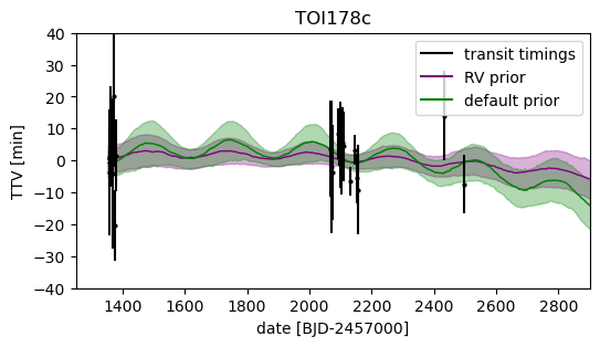
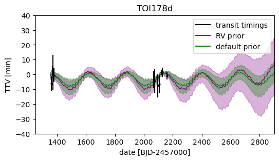
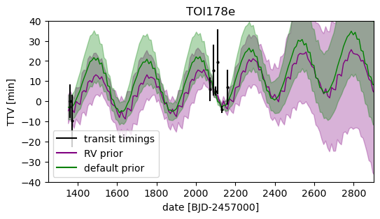
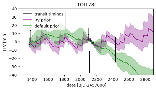
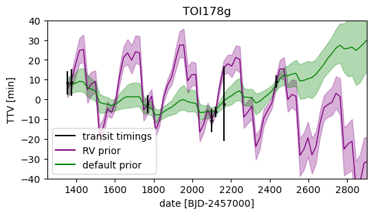
Figure 5: For each planet, the black points with error bars show the measured TTVs in minutes. For each planet, we also show the median and 1-sigma envelope for the TTVs propagated from 300 randomly-selected samples of the posterior obtained with the RV (purple) and default (green) mass priors.

We study here the transit timings reported in Table LABEL:tab:timings for the five outer planets. L21 predicted TTV peak-to-peak amplitudes ranging from several minutes for the inner planets to a few tens of minutes for the outer ones. Since the timing uncertainties of the inner planets are comparable to the expected signal, we proceed in two steps. First, we check whether the observed transit timings are consistent with the RV masses and if some constraints on the eccentricities can be obtained by combining the two. As a second step, we then assess the constraints on the masses that can be derived from the TTVs alone.

We fit the TTVs using the code presented in Leleu et al. (2021b): the transit timings are estimated using the TTVfast algorithm (Deck et al., 2014) and the samsam MCMC algorithm (see Delisle et al., 2018) is used to sample the posteriors. As L21 showed variations in the projected orbital inclination of only about 0.1 degree between the outer planets (Fig. 8 of L21), we assume in this study that the system is coplanar. The mean longitudes, periods, arguments of periastron, and eccentricities of the planets have uniform priors. For our first test, the mass priors are Gaussian with the respective mean and standard deviation based on the RV posteriors presented in L21. We call this setup the RV prior. The mass and eccentricity posteriors of this fit are shown in Fig. 4 and given in Table 9 (together with the RV mass priors for comparison). Fig. 4 shows that, for each planet, the mass posterior of the TTV fit is 1-$\sigma$ consistent with the RV prior, implying that the observed TTVs are indeed compatible with the RV masses. When using the RV mass priors, the TTVs allow us to constrain the eccentricities. L21 set the eccentricities to 0 as the available RVs did not allow a precise measurement, and the stability analysis of the system showed that the eccentricities had to be of a few percent at most. Here, the posteriors of the TTV fit obtained with the RV mass priors explore eccentricities that are consistent with both the masses determined from the RVs (all mass posteriors are 1-$\sigma$ consistent with their priors) and the TTV signals. We report the derived eccentricities in Tables 3 (planets $b$, $c$, and $d$) and 4 (planets $e$, $f$, and $g$). The 0.84 quantiles of the eccentricities are below 0.021 for all planets, which is consistent with the stability study of the system presented in L21.

As a second step, we check which constraints on the masses can be obtained from the TTVs alone. The main TTV signal whose period is the aforementioned super-period is degenerate between the planetary masses and eccentricities (Lithwick et al., 2012). The observation of other TTV harmonics, such as the chopping signal or the resonant evolution of the Laplace angle is thus necessary to constrain the planetary masses. Following Hadden & Lithwick (2016, 2017), we hence fit the data with different mass priors to test the robustness of the retrieved masses. The default prior is log-uniform in planetary masses, while the high-mass prior is uniform in planetary masses. Posteriors that we obtained using these priors are also shown in Fig. 4. We quantify the robustness of the mass determination using the parameter:

$$\Delta_{M}=\left|\frac{M_{\text{default}}^{.5}-M_{\text{high-mass}}^{.5}}{M_{\text{default}}^{.84}-M_{\text{default}}^{.5}}\right|$$ (3)

where $M_{\text{default}}^{.5}$ is the quantile at .5 of the default mass posterior, and similarly for other quantities. The robustness mass criterion from Hadden & Lithwick (2017) requires that $\Delta_{M}<1$ (note that their criterion is even more conservative as their high-mass prior also contains a log-uniform eccentricity prior, while in our case the eccentricity prior is uniform for all posteriors). The values that we obtained for $\Delta_{M}$, reported in Table 9, imply that the mass estimations of planets $c$, $f$, and $g$ are highly degenerate ($\Delta_{M}>3$ for the three of them). The test finds robust masses for planets $d$ and $e$. For TOI-178 e, the medians of both the default and high-mass posteriors are within 1-$\sigma$ of the RV prior, while for TOI-178 d, the medians of the two posteriors are both outside the 1-$\sigma$ interval of the RV prior.

However, the mean log-Likelihood computed for each posterior differs by less than 1 across all three. It implies that the three solutions explain the data equally well and that the various priors explore different parts of the underlying degeneracies. As a result, we recommend keeping for now the RV mass estimates presented in L21 as nominal values for the masses of the planets, as we deem the current TTV mass posteriors too much prior-dependent. Nonetheless, the apparent mass shift between the RV prior and the higher mass posterior found with both the default and high-mass priors for TOI-178 d highlights the importance of continuing to monitor the system in the future, both in RVs and TTVs. Indeed, TOI-178 d had been found by L21 to have a surprisingly low density based on its RV mass estimate (Sect. 1). Differences in planet density between RV- and TTV-characterised systems have been discussed in numerous studies over the last decade (e.g. Hadden & Lithwick, 2017; Mills & Mazeh, 2017; Leleu et al., 2023). TOI-178 offers the rare opportunity to compare the two techniques for the same system.

Fig. 5 shows the measured transit timings, as well as the TTV posteriors obtained with the RV (purple) and default (green) mass priors. We note that all current TTV measurements are well explained by the known planets of the system. The TTV signal over the $\sim$260d super-period is clearly visible in the posteriors of all planets. For the RV prior, a strong chopping signal is also visible for the two outer planets, while for the default prior, the TTVs are explained mainly through the slow evolution of the Laplace angles. A two-year projection after the last observed transit shows that future observations should be able to distinguish between these solutions.

Finally, we note that a photodynamical analysis of the light curves, where the gravitational interactions between the planets are taken into account at the stage of the light curve modelling (e.g. Ragozzine & Holman, 2010; Almenara et al., 2018, 2022), could help to better constrain the orbital parameters and masses. In particular, it has been shown that a photodynamical analysis can help to reduce the mass-eccentricity degeneracy when compared to the fit of pre-extracted transit timings, in particular for planets in the super-Earth to mini-Neptune range (Leleu et al., 2023). Such a photodynamical analysis will be performed in an upcoming paper (Leleu et al. 2023, in prep.).

6 Conclusions

In this work, we presented a detailed photometric study of the TOI-178 system, based on 40 new CHEOPS visits, one new TESS sector, as well as previously published data. We first performed a global analysis of the 100 transits contained in these data. This enabled us to significantly refine the transit parameters of the six TOI-178 planets, most notably their radii, for which we obtain relative precisions $\lesssim$3%, with the exception of the smallest planet $b$ for which the precision is 5.1%. We also used our extensive photometric dataset to place constraints on the radii and orbital periods of potential additional transiting planets in the system.

As part of our study, we also performed a first dynamical analysis of the TTVs measured for the five outer planets ($c$ to $g$), testing different priors for their masses to assess the robustness of the derived solution. We found that the mass posteriors are very prior-dependent. On one hand, when fitting the TTVs with mass priors based on the previously-published RVs, we find masses that are consistent with the RVs, and eccentricities that are all below 0.02, as expected from stability requirements. On the other hand, when fitting the TTVs with uniform or log-uniform (RV-independent) mass priors, we find mass estimates that are highly degenerate for planets $c$, $f$, and $g$; consistent with the RVs for planet $e$; and higher than the RV mass for planet $d$. We note that this latter planet had been found by L21 to have a surprisingly low density based on its RV mass estimate. Since the masses derived from the current TTV dataset are very prior-dependent, we recommend keeping for now the RV mass estimates presented in L21 as nominal values for the masses of the planets. Altogether, this first TTV study highlights the importance of continuing to monitor the system in the future, both in RVs and TTVs. In this context, further TTV measurements with CHEOPS and TESS (TOI-178 will be observed again in Sector 69), covering a longer temporal baseline, should help to break the degeneracies and improve our understanding of this benchmark planetary system.

Appendix A Data: CHEOPS visits

Table 5: Log of the CHEOPS observations. The file key (first column) is a unique identifier that can be used to retrieve the data from the CHEOPS archive. The efficiency (sixth column) represents the ratio between the amount of science observing time in a visit (excluding the interruptions due to Earth occultations or SAA crossings) and the total duration of the visit (including interruptions). The last two columns give the median absolute deviation (MAD) of the difference between two consecutive data points of the light curve for the CHEOPS Data Reduction Pipeline (DRP) and the PSF photometry pipeline (PIPE).

File key	UTC start	UTC end	Content	$N_{\mathrm{frames}}$	Efficiency	DRP MAD	PIPE MAD
					(%)	(ppm)	(ppm)
PR100031_TG028901	2020-07-21 11:01	2020-07-21 14:28	Filler	112	54.1	632	485
PR100031_TG029001	2020-07-25 01:59	2020-07-25 05:13	Filler	109	56.2	598	550
PR100031_TG030201(a)	2020-08-04 22:10	2020-08-09 01:57	b ($\times$2), c, d, e	3253	54.3	662	590
PR100031_TG030301(a)	2020-08-09 02:47	2020-08-15 22:50	b ($\times$4), c ($\times$2), d	5590	56.8	665	590
PR100031_TG030701(a)	2020-09-07 08:06	2020-09-07 21:27	e, g	559	69.7	740	638
PR100031_TG032101	2020-09-20 21:02	2020-09-21 01:54	Filler	257	87.7	741	596
PR100031_TG031001	2020-09-22 21:02	2020-09-23 00:15	Filler	165	85.0	648	583
PR100031_TG031801	2020-09-23 00:26	2020-09-23 05:18	Filler	283	96.5	747	532
PR100031_TG032201	2020-09-28 03:51	2020-09-28 12:17	b, d, g	441	86.9	759	657
PR100031_TG031101	2020-09-29 06:23	2020-09-29 11:24	Filler	253	83.7	631	638
PR100031_TG031201	2020-10-01 07:32	2020-10-01 10:45	Filler	160	82.4	1016	650
PR100031_TG031401	2020-10-03 10:24	2020-10-03 13:37	Filler	180	92.7	879	664
PR100031_TG033301(a)	2020-10-03 18:51	2020-10-04 02:51	b, f	424	88.1	750	593
PR100031_TG031301	2020-10-04 17:02	2020-10-04 19:59	Filler	161	90.4	798	583
PR100031_TG033001	2020-10-04 20:26	2020-10-05 05:09	d	480	91.6	686	550
PR100031_TG033302	2020-10-05 16:42	2020-10-05 23:56	b	379	87.1	825	574
PR100031_TG033101	2020-10-07 06:05	2020-10-07 15:26	c, e	497	88.4	762	604
PR100031_TG033303	2020-10-07 15:37	2020-10-07 22:51	b	372	85.5	844	613
PR100031_TG031901	2020-10-08 22:04	2020-10-09 02:56	Filler	273	93.1	687	602
PR100031_TG032001	2020-10-09 08:10	2020-10-09 13:02	Filler	254	86.6	737	571
PR100031_TG033304	2020-10-09 13:13	2020-10-09 20:20	b	399	93.2	755	593
PR100031_TG033901	2020-10-12 18:09	2020-10-12 23:27	Filler	236	73.9	782	609
PR100031_TG035101	2020-10-19 02:36	2020-10-19 10:20	b, f	333	71.6	734	617
PR100031_TG033902	2020-10-20 00:21	2020-10-20 05:13	Filler	218	74.4	927	633
PR100031_TG034001	2020-10-21 11:19	2020-10-21 14:32	Filler	131	67.5	657	464
PR100031_TG033903	2020-10-22 11:52	2020-10-22 16:41	Filler	193	66.5	796	605
PR100031_TG034201	2020-10-23 15:18	2020-10-23 22:52	c	262	57.6	759	669
PR100031_TG034002	2020-10-24 20:59	2020-10-24 23:52	Filler	97	55.7	892	593
PR100031_TG033904	2020-10-26 06:00	2020-10-26 10:53	Filler	174	59.4	595	469
PR100031_TG034003	2020-10-28 01:30	2020-10-28 04:43	Filler	115	59.3	756	593
PR100031_TG035601	2020-10-28 17:17	2020-10-29 00:16	b	115	59.3	841	736
PR100031_TG033905	2020-10-29 20:30	2020-10-30 01:33	Filler	153	50.3	712	581
PR100031_TG035701	2020-10-30 02:16	2020-10-30 09:46	c	285	63.2	723	647
PR100031_TG035702	2020-11-02 08:03	2020-11-02 16:07	c	274	56.5	715	634
PR100031_TG036101	2020-11-03 07:32	2020-11-03 14:19	b, f	234	57.3	627	614
PR100031_TG036401	2020-11-06 04:41	2020-11-06 14:02	e	289	51.4	644	517
PR100031_TG036301	2020-11-06 14:13	2020-11-06 22:56	d	240	45.8	675	558
PR100031_TG035602	2020-11-07 07:09	2020-11-07 13:55	b	234	57.5	714	626
PR100031_TG036201	2020-11-08 14:11	2020-11-08 22:13	g	218	45.1	766	577
PR100031_TG043601	2021-08-04 09:14	2021-08-04 18:48	b, c, f	306	53.2	691	618
PR100031_TG043701	2021-08-04 19:00	2021-08-05 05:53	c, g	360	55.0	740	668
PR100031_TG043201	2021-10-08 06:52	2021-10-08 14:01	b, c	378	87.9	682	602
PR100031_TG043202	2021-10-15 22:47	2021-10-16 05:56	b	343	79.7	650	552
PR100031_TG043203	2021-10-17 21:29	2021-10-18 04:38	b	304	70.7	679	587

Notes. ^(a) Data previously presented in L21.

Appendix B Global transit analysis: supplementary material

B.1 Photometric baseline models and error scaling factors

Date	Facility	Planet(s)	Epoch(s)	$N_{\rm points}$	$T_{\rm exp}$	Baseline model	Residual RMS	$\beta_{w}$	$\beta_{r}$
(UT)					(s)		(%)
2018-09-23	TESS	g	-26	265	120	$o$	0.118	0.94	1.74
2018-08-24	TESS	b	-301	196	120	$o$	0.118	0.94	1.29
2018-08-26	TESS	c	-176	218	120	$o$	0.121	0.96	1.23
2018-08-26	TESS	b	-300	195	120	p($t$)	0.116	0.92	1.14
2018-08-28	TESS	b	-299	187	120	$o$	0.123	0.97	1.48
2018-08-28	TESS	c	-175	228	120	$o$	0.126	1.00	1.08
2018-08-29	TESS	d	-61	247	120	p($t$)	0.127	1.01	1.08
2018-08-30	TESS	b	-298	197	120	$o$	0.108	0.86	1.00
2018-08-31	TESS	b, c	-297, -174	229	120	$o$	0.119	0.94	1.15
2018-09-01	TESS	e	-40	293	120	$o$	0.114	0.90	1.09
2018-09-02	TESS	b	-296	195	120	$o$	0.118	0.93	1.00
2018-09-03	TESS	f	-35	283	120	$o$	0.125	0.97	1.13
2018-09-04	TESS	c	-173	227	120	$o$	0.118	0.92	1.35
2018-09-04	TESS	b	-295	193	120	$o$	0.135	1.05	1.28
2018-09-05	TESS	d	-60	235	120	$o$	0.108	0.84	1.07
2018-09-07	TESS	c	-172	229	120	$o$	0.133	1.05	1.65
2018-09-08	TESS	b	-293	202	120	$o$	0.118	0.94	1.33
2018-09-10	TESS	b	-292	196	120	$o$	0.129	1.02	1.36
2018-09-10	TESS	c	-171	225	120	$o$	0.119	0.94	1.33
2018-09-11	TESS	e	-39	296	120	$o$	0.126	1.00	1.79
2018-09-11	TESS	d	-59	239	120	$o$	0.120	0.95	1.47
2018-09-12	TESS	b	-291	190	120	$o$	0.111	0.88	1.71
2018-09-13	TESS	g	-25	265	120	$o$	0.122	0.97	1.65
2018-09-13	TESS	c	-170	226	120	$o$	0.122	0.97	1.00
2018-09-14	TESS	b	-290	186	120	$o$	0.111	0.88	1.47
2018-09-16	TESS	b	-289	186	120	$o$	0.132	1.04	1.59
2018-09-17	TESS	c	-169	206	120	$o$	0.117	0.92	1.65
2018-09-18	TESS	b	-288	195	120	$o$	0.121	0.94	1.20
2018-09-18	TESS	d	-58	173	120	$o$	0.129	1.00	1.02
2018-09-18	TESS	f	-34	268	120	$o$	0.130	1.00	1.11
2019-09-11	NGTS1	b	-101	2321	10	p($a$)	0.639	0.72	1.13
2019-09-11	NGTS2	b	-101	2332	10	p($a$)	0.627	0.75	1.23
2019-09-11	NGTS3	b	-101	2326	10	p($a$)	0.634	0.76	1.48
2019-09-11	NGTS4	b	-101	2325	10	p($a$)	0.633	0.74	1.01
2019-09-11	NGTS5	b	-101	2330	10	p($a$)	0.637	0.75	1.46
2019-09-11	NGTS6	b	-101	2309	10	p($a$)	0.639	0.78	1.96
2019-10-12	NGTS1	g	-6	1835	10	p($a$)	0.578	0.60	2.74
2019-10-12	NGTS2	g	-6	1828	10	p($a$)	0.581	0.60	1.46
2019-10-12	NGTS3	g	-6	1838	10	p($a$)	0.616	0.61	1.11
2019-10-12	NGTS4	g	-6	1823	10	p($a$)	0.553	0.56	1.42
2019-10-12	NGTS5	g	-6	1836	10	p($a$)	0.574	0.60	1.00
2019-10-12	NGTS6	g	-6	1849	10	p($a$)	0.567	0.59	2.23
2019-10-12	NGTS7	g	-6	1831	10	p($a$)	0.578	0.59	1.65
2020-08-05	CHEOPS	b	71	206	60	sp($r$) + $o$	0.057	1.01	1.28
2020-08-06	CHEOPS	c, d	44, 47	404	60	sp($r$) + $o$	0.057	1.00	2.49
2020-08-07	CHEOPS	b	72	190	60	sp($r$) + $o$	0.057	1.00	1.55
2020-08-08	CHEOPS	e	31	331	60	sp($r$) + $o$	0.057	1.00	2.11
2020-08-09	CHEOPS	b	73	196	60	sp($r$) + $o$	0.060	1.07	1.83
2020-08-10	CHEOPS	c	45	185	60	sp($r$) + $o$	0.056	1.00	1.07
2020-08-11	CHEOPS	b	74	187	60	sp($r$) + $o$	0.056	1.00	1.92
2020-08-12	CHEOPS	b	75	275	60	sp($r$) + $o$	0.056	1.01	2.23
2020-08-13	CHEOPS	c, d	46, 48	374	60	sp($r$) + p($b$)	0.058	1.04	2.14
2020-08-15	CHEOPS	b	76	279	60	sp($r$) + $o$	0.056	1.00	1.13
2020-08-28	TESS	b, e	83, 33	368	120	$o$	0.124	0.99	1.19
2020-08-29	TESS	c	51	241	120	$o$	0.124	0.99	1.00
2020-08-30	TESS	b	84	207	120	$o$	0.119	0.94	1.09
2020-09-01	TESS	b	85	208	120	$o$	0.122	0.97	1.26
2020-09-01	TESS	c	52	240	120	$o$	0.115	0.91	1.00
2020-09-02	TESS	d	51	236	120	$o$	0.131	1.04	1.08
2020-09-03	TESS	b	86	208	120	$o$	0.110	0.87	1.07
2020-09-03	TESS	f	13	288	120	$o$	0.112	0.88	1.32
2020-09-04	TESS	b, c	87, 53	361	120	$o$	0.120	0.93	1.50
2020-09-07	CHEOPS	e, g	34, 10	555	60	sp($r$) + p($t$)	0.060	1.06	1.71
2020-09-10	TESS	b	90	207	120	$o$	0.131	1.03	1.48
2020-09-11	TESS	c	55	238	120	$o$	0.124	0.98	1.56
2020-09-12	TESS	b	91	207	120	$o$	0.115	0.91	1.25
2020-09-14	TESS	b	92	195	120	$o$	0.120	0.95	1.34
2020-09-14	TESS	c	56	216	120	$o$	0.126	0.99	1.26
2020-09-15	TESS	d	53	287	120	$o$	0.138	1.09	1.24
2020-09-16	TESS	b	93	207	120	$o$	0.135	1.07	1.33
2020-09-17	TESS	e	35	308	120	$o$	0.129	1.02	1.03
2020-09-18	TESS	c	57	240	120	$o$	0.122	0.96	1.00
2020-09-18	TESS	b	94	207	120	$o$	0.116	0.91	1.48
2020-09-18	TESS	f	14	267	120	$o$	0.125	0.98	1.37
2020-09-28	CHEOPS	b, d, g	99, 55, 11	434	60	sp($r$) + p($b$)	0.061	1.05	1.16
2020-10-03	CHEOPS	b, f	102, 15	426	60	sp($r$) + p($y$)	0.057	1.02	1.25
2020-10-04	CHEOPS	d	56	483	60	sp($r$) + p($b$)	0.059	1.05	2.19
2020-10-05	CHEOPS	b	103	365	60	sp($r$) + p($b$)	0.057	1.01	1.31
2020-10-07	CHEOPS	c, e	63, 37	486	60	sp($r$) + p($y$)	0.059	1.05	1.27
2020-10-07	CHEOPS	b	104	374	60	sp($r$) + $o$	0.056	1.00	1.58
2020-10-09	CHEOPS	b	105	394	60	sp($r$) + $o$	0.058	1.04	1.03
2020-10-19	CHEOPS	b, f	110, 16	329	60	sp($r$) + p($t$)	0.057	1.02	1.27
2020-10-23	CHEOPS	c	68	258	60	sp($r$) + p($t$)	0.061	1.08	1.16
2020-10-28	CHEOPS	b	115	205	60	sp($r$) + $o$	0.062	1.11	1.36
2020-10-30	CHEOPS	c	70	282	60	sp($r$) + p($ttt$)	0.060	1.07	1.68
2020-11-02	CHEOPS	c	71	268	60	sp($r$) + p($t$)	0.061	1.09	1.75
2020-11-03	CHEOPS	b, f	118, 17	233	60	sp($r$) + p($ttt$)	0.057	1.00	1.49
2020-11-06	CHEOPS	e	40	297	60	sp($r$) + $o$	0.056	1.00	1.84
2020-11-06	CHEOPS	d	61	247	60	sp($r$) + $o$	0.059	1.06	1.90
2020-11-07	CHEOPS	b	120	229	60	sp($r$) + $o$	0.060	1.08	1.41
2020-11-08	CHEOPS	g	13	223	60	sp($r$) + $o$	0.056	1.00	2.56
2021-08-04	CHEOPS	b, f, c	261, 35, 156	293	60	sp($r$) + $o$	0.063	1.12	2.10
2021-08-04	CHEOPS	c, g	156, 26	343	60	sp($r$) + p($y$)	0.066	1.18	1.48
2021-10-08	CHEOPS	b, c	295, 176	365	60	sp($r$) + $o$	0.057	1.01	2.66
2021-10-15	CHEOPS	b	299	327	60	sp($r$) + $o$	0.058	1.01	1.47
2021-10-17	CHEOPS	b	300	296	60	sp($r$) + $o$	0.067	1.15	1.43

Table 6: Photometric baseline models, residual RMS, and error scaling factors $\beta_{w}$ and $\beta_{r}$ for each transit light curve used in our global transit analysis (see Sect. 4.1). For the baseline function, $o$ is a simple constant (to account for any out-of-transit flux offset), sp($r$) is a cubic spline against the spacecraft roll angle $r$, and p($\alpha$) denotes a first-order polynomial function of the parameter $\alpha$, with $\alpha$ that can be $t=$ time, $b=$ background, $a=$ airmass, $x$ and $y=$ $x$- and $y$- position of the target on the detector, or $ttt=$ telescope tube temperature. Epochs are relative to the updated mean transit ephemerides given in Tables 3 (planets $b$, $c$, and $d$) and 4 (planets $e$, $f$, and $g$).

B.2 Prior distributions

Parameter (unit)	Prior
Mass, $M_{\star}$ ($M_{\odot}$)	$\mathcal{N}$(0.647, 0.0302)
Radius, $R_{\star}$ ($R_{\odot}$)	$\mathcal{N}$(0.662, 0.0102)
Effective temperature, $T_{\mathrm{eff}}$ (K)	$\mathcal{N}$(4316, 702)
Quadratic limb-darkening coefficient $u_{1,\>\mathrm{CHEOPS}}$	$\mathcal{N}$(0.538, 0.0232)
Quadratic limb-darkening coefficient $u_{2,\>\mathrm{CHEOPS}}$	$\mathcal{N}$(0.157, 0.0332)
Quadratic limb-darkening coefficient $u_{1,\>\mathrm{TESS}}$	$\mathcal{N}$(0.487, 0.0192)
Quadratic limb-darkening coefficient $u_{2,\>\mathrm{TESS}}$	$\mathcal{N}$(0.193, 0.0472)
Quadratic limb-darkening coefficient $u_{1,\>\mathrm{NGTS}}$	$\mathcal{N}$(0.529, 0.0302)
Quadratic limb-darkening coefficient $u_{2,\>\mathrm{NGTS}}$	$\mathcal{N}$(0.171, 0.0452)

Table 7: Prior probability distribution functions assumed in our global transit analysis (see Sect. 4.1). $\mathcal{N}(\mu,\sigma^{2})$ represents a normal distribution of mean $\mu$ and variance $\sigma^{2}$.

Appendix C Results: individual transit timings

Epoch	Transit timing	TTV	Source
	($\mathrm{BJD_{TDB}}-2\,450\,000$)	(minutes)
TOI-178 c
-176	$8356.0989_{-0.0138}^{+0.0080}$	$-2.89_{-19.87}^{+11.53}$	TESS
-175	$8359.3408_{-0.0050}^{+0.0061}$	$2.09_{-7.21}^{+8.76}$	TESS
-174	$8362.5850_{-0.0095}^{+0.0086}$	$10.29_{-13.75}^{+12.43}$	TESS
-173	$8365.8208_{-0.0078}^{+0.0096}$	$6.56_{-11.29}^{+13.82}$	TESS
-172	$8369.052_{-0.013}^{+0.016}$	$-3.38_{-19.30}^{+23.47}$	TESS
-171	$8372.308_{-0.015}^{+0.011}$	$21.06_{-22.18}^{+16.42}$	TESS
-170	$8375.5181_{-0.0052}^{+0.0077}$	$-19.55_{-7.53}^{+11.10}$	TESS
-169	$8378.7718_{-0.0077}^{+0.0075}$	$2.43_{-11.16}^{+10.77}$	TESS
44	$9068.5625_{-0.0086}^{+0.0104}$	$4.00_{-12.40}^{+14.98}$	CHEOPS
45	$9071.797_{-0.012}^{+0.014}$	$-1.78_{-17.28}^{+20.74}$	CHEOPS
46	$9075.034_{-0.010}^{+0.008}$	$-3.44_{-14.98}^{+11.49}$	CHEOPS
51	$9091.2349_{-0.0055}^{+0.0047}$	$8.67_{-7.99}^{+6.78}$	TESS
52	$9094.4701_{-0.0038}^{+0.0026}$	$3.99_{-5.47}^{+3.74}$	TESS
53	$9097.7094_{-0.0094}^{+0.0082}$	$5.20_{-13.55}^{+11.88}$	TESS
55	$9104.1840_{-0.0076}^{+0.0086}$	$1.86_{-11.00}^{+12.36}$	TESS
56	$9107.4252_{-0.0077}^{+0.0073}$	$5.81_{-11.10}^{+10.56}$	TESS
57	$9110.6629_{-0.0050}^{+0.0075}$	$4.74_{-7.16}^{+10.81}$	TESS
63	$9130.0860_{-0.0018}^{+0.0031}$	$-6.21_{-2.62}^{+4.46}$	CHEOPS
68	$9146.2850_{-0.0029}^{+0.0033}$	$3.59_{-4.18}^{+4.77}$	CHEOPS
70	$9152.7557_{-0.0049}^{+0.0053}$	$-5.30_{-7.07}^{+7.70}$	CHEOPS
71	$9155.9917_{-0.0097}^{+0.0089}$	$-8.88_{-14.00}^{+12.76}$	CHEOPS
156	$9431.2758_{-0.0069}^{+0.0098}$	$14.06_{-9.92}^{+14.05}$	CHEOPS
176	$9496.0299_{-0.0056}^{+0.0065}$	$-7.38_{-8.02}^{+9.30}$	CHEOPS
TOI-178 d
-61	$8360.2385_{-0.0026}^{+0.0033}$	$-6.00_{-3.72}^{+4.82}$	TESS
-60	$8366.8025_{-0.0021}^{+0.0020}$	$2.97_{-3.02}^{+2.84}$	TESS
-59	$8373.3593_{-0.0082}^{+0.0040}$	$1.58_{-11.88}^{+5.82}$	TESS
-58	$8379.9157_{-0.0028}^{+0.0033}$	$-0.27_{-4.02}^{+4.72}$	TESS
47	$9068.4744_{-0.0029}^{+0.0039}$	$-3.27_{-4.16}^{+5.63}$	CHEOPS
48	$9075.0314_{-0.0055}^{+0.0039}$	$-4.22_{-7.92}^{+5.56}$	CHEOPS
51	$9094.7023_{-0.0055}^{+0.0036}$	$-7.51_{-7.92}^{+5.13}$	TESS
53	$9107.8186_{-0.0043}^{+0.0040}$	$-6.24_{-6.25}^{+5.75}$	TESS
55	$9120.9395_{-0.0013}^{+0.0012}$	$1.58_{-1.83}^{+1.73}$	CHEOPS
56	$9127.4973_{-0.0022}^{+0.0022}$	$1.74\pm 3.17$	CHEOPS
61	$9160.2843_{-0.0018}^{+0.0016}$	$-0.70_{-2.64}^{+2.30}$	CHEOPS
TOI-178 e
-40	$8362.9541_{-0.0031}^{+0.0058}$	$0.07_{-4.51}^{+8.29}$	TESS
-39	$8372.9091_{-0.0091}^{+0.0085}$	$-9.80_{-13.05}^{+12.25}$	TESS
31	$9070.2469_{-0.0039}^{+0.0041}$	$5.65_{-5.66}^{+5.88}$	CHEOPS
33	$9090.1771_{-0.0087}^{+0.0077}$	$15.11_{-12.60}^{+11.16}$	TESS
34	$9100.1317_{-0.0014}^{+0.0016}$	$4.77_{-1.96}^{+2.28}$	CHEOPS
35	$9110.1036_{-0.0112}^{+0.0087}$	$19.29_{-16.13}^{+12.54}$	TESS
37	$9130.0109_{-0.0012}^{+0.0012}$	$-4.29_{-1.70}^{+1.71}$	CHEOPS
40	$9159.9040_{-0.0054}^{+0.0061}$	$6.72_{-7.78}^{+8.80}$	CHEOPS
TOI-178 f
-35	$8364.9143_{-0.0041}^{+0.0039}$	$-3.41_{-5.92}^{+5.57}$	TESS
-34	$8380.1582_{-0.0101}^{+0.0090}$	$13.87_{-14.54}^{+12.99}$	TESS
13	$9096.0564_{-0.0051}^{+0.0056}$	$8.78_{-7.39}^{+8.02}$	TESS
14	$9111.2650_{-0.0056}^{+0.0092}$	$-24.86_{-7.99}^{+13.31}$	TESS
15	$9126.5155_{-0.0012}^{+0.0015}$	$1.90_{-1.70}^{+2.22}$	CHEOPS
16	$9141.7445_{-0.0029}^{+0.0033}$	$-2.36_{-4.12}^{+4.74}$	CHEOPS
17	$9156.9773_{-0.0015}^{+0.0016}$	$-1.13_{-2.20}^{+2.25}$	CHEOPS
35	$9431.1468_{-0.0103}^{+0.0093}$	$-9.23_{-14.83}^{+13.35}$	CHEOPS
TOI-178 g
-26	$8354.5502_{-0.0041}^{+0.0038}$	$8.97_{-5.89}^{+5.46}$	TESS
-25	$8375.2603_{-0.0046}^{+0.0045}$	$9.30_{-6.64}^{+6.51}$	TESS
-6	$8768.7409_{-0.0031}^{+0.0029}$	$-1.81_{-4.49}^{+4.18}$	NGTS
10	$9100.0936_{-0.0025}^{+0.0041}$	$-10.13_{-3.60}^{+5.93}$	CHEOPS
11	$9120.8067_{-0.0014}^{+0.0018}$	$-5.61_{-2.07}^{+2.64}$	CHEOPS
13	$9162.2292_{-0.0118}^{+0.0131}$	$-1.65_{-16.99}^{+18.86}$	CHEOPS
26	$9431.4659_{-0.0022}^{+0.0020}$	$9.74_{-3.18}^{+2.87}$	CHEOPS

Table 8: Individual transit timings returned by our global transit analysis (see Sect. 4.1) for the five outer TOI-178 planets. The epochs and corresponding TTVs given here are relative to the updated mean transit ephemerides given in Tables 3 (planets $b$, $c$, and $d$) and 4 (planets $e$, $f$, and $g$).

Appendix D Dynamical analysis: TTV mass and eccentricity posteriors for different mass priors

Table 9: TTV mass and eccentricity posteriors for the 5 outer planets of the TOI-178 system.

	Source	Prior	TOI-178 c	TOI-178 d	TOI-178 e	TOI-178 f	TOI-178 g
$M_{\mathrm{p}}$ [$M_{\oplus}$]	RVs (Leleu et al. 2021a)	–	$4.77\pm 0.68$	$3.01\pm 1.03$	$3.86\pm 1.25$	$7.72\pm 1.67$	$3.94\pm 1.62$
$M_{\mathrm{p}}$ [$M_{\oplus}$]	TTVs	RV	$4.70_{-0.63}^{+0.63}$	$3.35_{-0.79}^{+0.81}$	$3.11_{-0.87}^{+0.96}$	$7.50_{-1.18}^{+1.27}$	$3.12_{-1.11}^{+1.10}$
$M_{\mathrm{p}}$ [$M_{\oplus}$]	TTVs	default	$0.22_{-0.17}^{+0.78}$	$7.73_{-1.71}^{+2.09}$	$3.61_{-1.13}^{+1.31}$	$0.78_{-0.59}^{+0.99}$	$0.17_{-0.12}^{+0.51}$
$M_{\mathrm{p}}$ [$M_{\oplus}$]	TTVs	high-mass	$8.08_{-5.26}^{+7.98}$	$8.33_{-2.23}^{+2.33}$	$3.12_{-1.45}^{+1.64}$	$6.76_{-2.51}^{+2.62}$	$1.88_{-1.19}^{+1.47}$
$\Delta_{M}$	Robustness criterion	–	$10.08$	$0.29$	$0.37$	$6.06$	$3.34$
$e_{\mathrm{p}}$	TTVs	RV	$0.0073_{-0.0051}^{+0.0083}$	$0.010_{-0.007}^{+0.011}$	$0.0080_{-0.0057}^{+0.0100}$	$0.0105_{-0.0061}^{+0.0071}$	$0.0056_{-0.0039}^{+0.0058}$
$e_{\mathrm{p}}$	TTVs	default	$0.0071_{-0.0050}^{+0.0081}$	$0.0051_{-0.0036}^{+0.0067}$	$0.0041_{-0.0029}^{+0.0054}$	$0.012_{-0.008}^{+0.016}$	$0.022_{-0.016}^{+0.027}$
$e_{\mathrm{p}}$	TTVs	high-mass	$0.0033_{-0.0023}^{+0.0038}$	$0.0049_{-0.0034}^{+0.0055}$	$0.0050_{-0.0035}^{+0.0057}$	$0.0068_{-0.0045}^{+0.0065}$	$0.0039_{-0.0028}^{+0.0045}$