Strong limit theorems for empirical halfspace depth trimmed regions

Abstract.

We study empirical variants of the halfspace (Tukey) depth of a probability measure $\mu$, which are obtained by replacing $\mu$ with the corresponding weighted empirical measure. We prove analogues of the Marcinkiewicz–Zygmund strong law of large numbers and of the law of the iterated logarithm in terms of set inclusions and for the Hausdorff distance between the theoretical and empirical variants of depth trimmed regions. In the special case of $\mu$ being the uniform distribution on a convex body $K$, the depth trimmed regions are convex floating bodies of $K$, and we obtain strong limit theorems for their empirical estimators.

1

1. Introduction

The halfspace depth of a point $x\in\mathbb{R}^{d}$ with respect to a Borel probability measure $\mu$ on $\mathbb{R}^{d}$, also called the depth function, is defined as

$$D(x)=\inf\{\mu(H)\colon H\in\mathcal{H},H\ni x\},\quad x\in\mathbb{R}^{d},$$ (1.1)

where $\mathcal{H}$ is the family of all closed halfspaces in $\mathbb{R}^{d}$. A generic halfspace is denoted by $H$ and its boundary by $\partial H$, which is $(d-1)$-dimensional affine subspace. In other words, the depth of $x$ is the smallest measure of a halfspace containing $x$. Clearly, the infimum in (1.1) can be equivalently taken over all $H$ with $x\in\partial H$. This concept was first introduced by Tukey [23] and is also called the Tukey depth, see [17] for a survey of recent results and geometric connections. For $\alpha\in(0,1]$, define the depth trimmed region

$$\mathcal{R}(\alpha)=\{x\in\mathbb{R}^{d}\colon D(x)\geq\alpha\},$$

that is, $\mathcal{R}(\alpha)$ is the upper level set of the depth function. The regions $\mathcal{R}(\alpha)$ are nested (i.e., decreasing with respect to the set inclusion) compact convex subsets of $\mathbb{R}^{d}$, see Corollary after Proposition 1 in [18] and Proposition 5 therein. Note that $\mathcal{R}(\alpha)$ converges to the convex hull of the support of $\mu$ as $\alpha\downarrow 0$.

Obviously, $\mathcal{R}(\alpha)$ is either empty or a singleton when $\alpha>1/2$. Moreover, for any $\alpha$,

$$\mathcal{R}(\alpha)=\bigcap_{H\in\mathcal{H}\colon\mu(H)>1-\alpha}H,$$ (1.2)

see Proposition 6 and Corollary thereafter in [18].

An empirical version $\widehat{\mathcal{R}}_{n}(\alpha)$ of $\mathcal{R}(\alpha)$ is constructed by replacing $\mu$ with the weighted empirical measure

$$\widehat{\mu}_{n}=n^{-1}\sum_{i=1}^{n}\xi_{i}\,\delta_{X_{i}}\,,$$ (1.3)

where $\{X_{i},i\geq 1\}$ is a sequence of $\mu$-distributed independent random vectors, $\{\xi_{i},i\geq 1\}$ is a sequence of i.i.d. random variables with $\mathbf{E}\xi_{1}=1$ independent of $\{X_{i},i\geq 1\}$, and $\delta_{x}$ denotes the Dirac measure at $x\in\mathbb{R}^{d}$. In particular, $\widehat{\mu}_{n}(\mathbb{R}^{d})=n^{-1}\sum_{i=1}^{n}\xi_{i}=\bar{\xi}_{n}$, the sample mean of $\xi_{i}$. If the weights $\xi_{i}$ are chosen to be identically one, $\widehat{\mu}_{n}$ is the empirical measure, see, e.g., [22] or [24]. In general, $\widehat{\mu}_{n}$ might be also signed. The above construction of the depth function and the depth trimmed regions applied to the empirical measure $\widehat{\mu}_{n}$ yields the empirical depth and the empirical depth trimmed regions $\widehat{\mathcal{R}}_{n}(\alpha)$. It can be easily shown that (1.2) remains true for finite signed measures and is applicable to $\widehat{\mathcal{R}}_{n}(\alpha)$ and $\widehat{\mu}_{n}$ with $1-\alpha$ replaced by $\bar{\xi}_{n}-\alpha$.

Our results on convergence of empirical depth trimmed regions are split into two groups. The nearness of $\mathcal{R}(\alpha)$ and $\widehat{\mathcal{R}}_{n}(\alpha)$ can be assessed in the inclusion sense by sandwiching the empirical depth trimmed region between two versions $\mathcal{R}(\alpha^{\prime}_{n})$ and $\mathcal{R}(\alpha^{\prime\prime}_{n})$ with parameters $\alpha^{\prime}_{n}$ and $\alpha^{\prime\prime}_{n}$ which converge to $\alpha$ from below and above as $n\to\infty$. In this case, we study the asymptotics of differences between $\alpha^{\prime}_{n}$, $\alpha^{\prime\prime}_{n}$ and $\alpha$. Another way is to consider the asymptotical behaviour of the Hausdorff distance $\rho_{H}(\mathcal{R}(\alpha),\widehat{\mathcal{R}}_{n}(\alpha))$. Strong limit theorems in the metric sense typically require additional assumptions on $\mu$, which are of smoothness nature.

In the specific case when the measure $\mu$ is uniform on a convex body $K\subset\mathbb{R}^{d}$, the set $\mathcal{R}(\alpha)$ is the convex floating body of $K$ at level $\alpha V_{d}(K)$, where $V_{d}(\cdot)$ denotes the Lebesgue volume, see [17] and [20]. Then $\widehat{\mathcal{R}}_{n}(\alpha)$ becomes an empirical estimator of the convex floating body. The Hausdorff distance between $\widehat{\mathcal{R}}_{n}(\alpha)$ and $\mathcal{R}(\alpha)$ in this setting has been studied in [4], where concentration type results are obtained, proving an upper exponential bound on the tail of the Hausdorff distance. Our results complement this work. In particular, we show that empirical floating bodies approximate the theoretical one at the rate $(n^{-1}\log\log n)^{1/2}$, so that the rate $n^{-1/2}$ for the convergence in probability from [4, Corollary 2] does not hold almost surely. It is interesting that this rate does not depend on the dimension, while the rate of approximation of a $C^{2}$-smooth convex body $K$ by the convex hull of a uniform random sample in $K$ is $(n^{-1}\log n)^{2/(d+1)}$ and so depends on dimension, see [2, Theorem 6].

It should be noted that related problems can be considered also for unbounded measures. For example, for the Lebesgue measure on $\mathbb{R}_{+}^{d}$ and a variant of empirical depth trimmed regions derived from multiple sums on the integer lattice, the strong law of large numbers and the law of the iterated logarithm were obtained in [8].

The paper is organised as follows. Section 2 reminds basic properties of the depth and standard assumptions on the underlying probability measure. It also contains some necessary representations of the theoretical and empirical depth trimmed regions.

In Section 3, we prove almost sure convergence of the empirical halfspace depth trimmed regions towards the theoretical ones and establish the rate of this convergence in terms of the Marcinkiewicz–Zygmund law. Section 4 contains the law of the iterated logarithm. Both these sections present results in the inclusion setting. Among other methods, the proofs extensively use techniques from the theory of empirical measures.

Section 5 presents a deterministic result concerning asymptotics of the Hausdorff distance between two depth trimmed regions at close levels. Since depth trimmed regions appear as solutions of inequalities, we can take advantage of the approach used in [14] to handle this task. Assuming differentiability of the depth function, we determine its gradient in terms of the Radon transform of the underlying measure.

In Section 6, we prove the strong law of large numbers and the law of the iterated logarithm for the Hausdorff distance between $\widehat{\mathcal{R}}_{n}(\alpha)$ and $\mathcal{R}(\alpha)$. In Section 7, we present several examples.

Appendix contains some geometric results which make it possible to show that the depth function generated by the uniform distribution on a symmetric smooth strictly convex body is differentiable.

2. Basic properties of depth trimmed regions

We start by listing some conditions on the measure $\mu$ needed in what follows. The first two are quite standard.

1. $\mu(E)=0$ for each hyperplane $E$.

2. If $H_{1},H_{2}\in\mathcal{H}$ are disjoint with $\mu(H_{1}),\mu(H_{2})>0$, then $\mu(H_{1})+\mu(H_{2})<1$.

Condition (C1) holds if $\mu$ is absolutely continuous with respect to the $d$-dimensional Lebesgue measure. Under (C1), the infimum in (1.1) is attained at some (possibly not unique) minimal halfspace $H$, and the depth function $D$ is continuous in $x$, see Proposition 4.5 in [11] or Proposition 1 in [13].

Condition (C2) is usually called the contiguity of support. This means that the support of $\mu$ cannot be divided into two disjoint parts separated by a strip. Clearly, (C2) holds for $\mu$ with connected support. Under (C1) and (C2), the map $\alpha\mapsto\mathcal{R}(\alpha)$ is continuous in the Hausdorff metric $\rho_{H}$ on $\alpha\in(0,\alpha_{\max})$, where

$$\alpha_{\max}=\sup\{D(x)\colon x\in\mathbb{R}^{d}\},$$

see Theorem 1 in [17]. Under some additional conditions, the differentiability of the function $\rho_{H}(\mathcal{R}(\alpha),\mathcal{R}(\alpha+t))$ in $t$ is proved in Section 5.

In the following lemma, we give two further useful consequences of (C1) and (C2). For a set $K$ in $\mathbb{R}^{d}$ and $E=\partial H$ for a halfspace $H$, we say that $E$ is a supporting hyperplane of $K$ at $x\in\partial K$ if $x\in E$ and $K$ is contained in one of the two closed halfspaces bounded by $E$.

Lemma 2.1.

Under (C1), (C2), and for each $\alpha\in(0,\alpha_{\max})$,

1. $\partial\mathcal{R}(\alpha)=\{x\colon D(x)=\alpha\}$, which is the $\alpha$-level surface of the depth function $D$;

2. the boundary of each minimal halfspace $H$ at $x\in\partial\mathcal{R}(\alpha)$ is a supporting hyperplane of $\mathcal{R}(\alpha)$.

Proof.

If $x\in\partial\mathcal{R}(\alpha)$ then $x_{i}^{-}\to x$ and $x_{i}^{+}\to x$ for some sequences $\{x_{i}^{-},i\geq 1\}$ and $\{x_{i}^{+},i\geq 1\}$ with $D(x_{i}^{-})<\alpha$ and $D(x_{i}^{+})\geq\alpha$ for all $i$. Hence, $D(x)=\alpha$ by continuity of the depth function implied by (C1).

Conversely, if $D(x)=\alpha$ then $x\in\partial\mathcal{R}(\alpha)$ since, otherwise, we would have $x\in\mathcal{R}(\beta)$ for some $\beta>\alpha$ by continuity of $\mathcal{R}(\cdot)$ in the Hausdorff metric implied by (C1) and (C2). This contradicts to $D(x)=\alpha$.

Finally, if $\partial H$ does not support $\mathcal{R}(\alpha)$ then $G\subset H$ for some $G\in\mathcal{H}$ such that $\partial G$ supports $\mathcal{R}(\alpha)$ at some point $y\in\partial\mathcal{R}(\alpha)$. Hence $\mu(G)\geq D(y)=\alpha$. On the contrary, $G\subset H$ and (C2) yield $\mu(G)<\mu(H)=D(x)=\alpha$. ∎

In (1.2) and in a similar representation of $\widehat{\mathcal{R}}_{n}(\alpha)$, we deal with uncountable intersections of closed halfspaces. In case of $\widehat{\mathcal{R}}_{n}(\alpha)$, the condition $\widehat{\mu}_{n}(H)>\bar{\xi}_{n}-\alpha$ is a random event due to measurability of $\widehat{\mu}_{n}$. Hence, to guarantee the measurability of the intersection we should show that $\widehat{\mathcal{R}}_{n}(\alpha)$ are countably determined. This means that we can replace $\mathcal{H}$ in the above representation by a countable subclass $\mathcal{H}_{0}\subset\mathcal{H}$, and still almost surely obtain the same depth trimmed regions.

The family of halfspaces whose boundaries contain the origin can be parametrised as

$$H_{u}=\{z\in\mathbb{R}^{d}\colon\langle z,u\rangle\leq 0\},\quad u\in\SS^{d-1},$$

where $\SS^{d-1}$ stands for the unit sphere in $\mathbb{R}^{d}$. Each halfspace from $\mathcal{H}$ can be given as $H_{u}+x$ for some $x\in\mathbb{R}^{d}$ and $u\in\SS^{d-1}$ or as

$$H_{u}(t)=\{z\in\mathbb{R}^{d}\colon\langle z,u\rangle\leq t\},\quad u\in\SS^{d-1},\;t\in\mathbb{R}.$$

Lemma 2.2.

Let $\mathcal{H}_{0}$ be the family of halfspaces $H_{u}(t)$ for all rational numbers $t$ and all $u$ from a countable dense set on the unit sphere. If $\mu$ is either a probability measure or a signed measure with a finite support then

$$\mathcal{R}(\alpha)=\bigcap_{\begin{subarray}{c}H\in\mathcal{H}_{0}\colon\\ \mu(H)>\mu(\mathbb{R}^{d})-\alpha\end{subarray}}H.$$ (2.1)

In particular, $\widehat{\mathcal{R}}_{n}(\alpha)$ is a random closed set.

Proof.

It suffices to prove that

$$\bigcap_{\begin{subarray}{c}H\in\mathcal{H}\colon\\ \mu(H)>\mu(\mathbb{R}^{d})-\alpha\end{subarray}}H\supset\bigcap_{\begin{subarray}{c}H\in\mathcal{H}_{0}\colon\\ \mu(H)>\mu(\mathbb{R}^{d})-\alpha\end{subarray}}H,$$ (2.2)

since the opposite inclusion is obvious.

If $x$ does not belong to the left-hand side of (2.2), then $x\notin H$ for some $H\in\mathcal{H}$ such that $\mu(H)=\mu(\mathbb{R}^{d})-\alpha+\varepsilon$ with $\varepsilon>0$. If $\mu$ is a finitely supported signed measure then there exists an $H_{0}\in\mathcal{H}_{0}$ such that $x\notin H_{0}$ and $\mu(H)=\mu(H_{0})$. Hence, $x$ does not belong to the right-hand side of (2.2) as well.

Let $\mu$ be a probability measure. Consider a ball $B\subset\mathbb{R}^{d}$ such that $\mu(B^{c})<\varepsilon$, and choose a halfspace $H_{0}\in\mathcal{H}_{0}$ such that $x\notin H_{0}$ and $(H_{0}\cap B)\supset(H\cap B)$. Then the chain of inequalities

$$\mu(H_{0}) =\mu(H_{0}\cap B)+\mu(H_{0}\cap B^{c})\geq\mu(H\cap B)$$

$$=\mu(H)-\mu(H\cap B^{c})\geq\mu(H)-\mu(B^{c})>\mu(\mathbb{R}^{d})-\alpha+\varepsilon-\varepsilon=\mu(\mathbb{R}^{d})-\alpha$$

implies that $x$ does not belong to the right-hand side of (2.2). This proves the first claim.

Let $H(n,\alpha)$ be $H$ if $\widehat{\mu}_{n}(H)>\bar{\xi}_{n}-\alpha$ and $\mathbb{R}^{d}$ otherwise. By (2.1),

$$\widehat{\mathcal{R}}_{n}(\alpha)=\bigcap_{H\in\mathcal{H}_{0}}H(n,\alpha).$$

Since $H(n,\alpha)$ are simple random closed sets in the sense of [15, Definition 1.3.15], the second claim follows from Theorem 1.3.25(vii) therein. ∎

The following result clarifies the structure of empirical depth trimmed regions.

Lemma 2.3.

The boundary of the empirical depth trimmed region $\widehat{\mathcal{R}}_{n}(\alpha)$ is contained in the union of all affine subspaces generated by $i$-tuples of points from $\{X_{1},\dots,X_{n}\}$ with $i=1,\ldots,d$.

Proof.

Let $\mathcal{I}$ be the family of all subsets $I\subset\Xi_{n}=\{X_{1},\dots,X_{n}\}$ such that $I$ equals the intersection of its convex hull $\operatorname{conv}I$ with $\Xi_{n}$ and $n^{-1}\sum_{X_{i}\in I}\xi_{i}>\bar{\xi}_{n}-\alpha$.

If $I\in\mathcal{I}$ and $I\subset H$ for a halfspace $H$ and $H\cap(\Xi_{n}\setminus I)=\emptyset$, then $\widehat{\mu}_{n}(H)>\bar{\xi}_{n}-\alpha$. If $\widehat{\mu}_{n}(H)>\bar{\xi}_{n}-\alpha$ for a halfspace $H$, then $H\supset I$ for $I=H\cap\Xi_{n}\in\mathcal{I}$ and $H$ does not intersect $\Xi_{n}\setminus I$. Thus,

$$\widehat{\mathcal{R}}_{n}(\alpha) =\bigcap\{H\colon\widehat{\mu}_{n}(H)>\bar{\xi}_{n}-\alpha\}$$

$$=\bigcap\{H\colon H\supset I,H\cap(\Xi_{n}\setminus I)=\emptyset\;\text{for}\;I\in\mathcal{I}\}$$

$$=\bigcap_{I\in\mathcal{I}}\bigcap\{H\colon H\supset I,H\cap(\Xi_{n}\setminus I)=\emptyset\}.$$

Hence, the boundary of $\widehat{\mathcal{R}}_{n}(\alpha)$ is a subset of the union of boundaries of the sets

$$\bigcap\{H\colon H\supset I,H\cap(\Xi_{n}\setminus I)=\emptyset\}$$

for $I\in\mathcal{I}$, not to say for all subsets $I$ of $\Xi_{n}$. The statement now follows from the following lemma. ∎

Lemma 2.4.

If $I_{1}$ and $I_{2}$ are finite sets in $\mathbb{R}^{d}$ then the intersection $A$ of all halfspaces which contain $I_{1}$ and do not intersect $I_{2}$ is either $\mathbb{R}^{d}$ or has the boundary which is a subset of the union of all affine subspaces generated by $i$-tuples of points from $I_{1}\cup I_{2}$ with $i=1,\ldots,d$.

Proof.

If $\operatorname{conv}I_{1}\hskip 0.5pt\cap\hskip 0.5pt\operatorname{conv}I_{2}\neq\emptyset$, there are no halfspaces which contain $I_{1}$ and do not intersect $I_{2}$. In this case $A=\mathbb{R}^{d}$.

Assume that the convex hulls of $I_{1}$ and $I_{2}$ are disjoint. Then $a\notin A$ if and only if there exists an $H\in\mathcal{H}$ containing $\operatorname{conv}I_{1}$ which intersects neither $\operatorname{conv}I_{2}$ nor $a$, that is, does not intersect $\operatorname{conv}(\{a\}\cup I_{2})$. By the separation theorem, this is possible if and only if $\operatorname{conv}I_{1}$ and $\operatorname{conv}(\{a\}\cup I_{2})$ are disjoint. Hence, $a\in\partial A$ means that $\operatorname{conv}I_{1}$ touches $\operatorname{conv}(\{a\}\cup I_{2})$, and thus there is a face $F_{1}$ of $\operatorname{conv}I_{1}$ and a face $F_{2}$ of $\operatorname{conv}(\{a\}\cup I_{2})$ of dimensions $d_{1},d_{2}\leq d-1$, respectively, such that $F_{1}$ and $F_{2}$ lie on an affine subspace $E$ of dimension at most $d-1$ and $F_{1}\cap F_{2}\neq\emptyset$. Moreover, it follows from the assumption $\operatorname{conv}I_{1}\hskip 0.5pt\cap\hskip 0.5pt\operatorname{conv}I_{2}=\emptyset$ that $F_{2}$ has $a$ as one of its vertices.

Let $x\in F_{1}\cap F_{2}$. Then

$$\sum_{k=1}^{d_{1}}s_{k}x_{k}=x=t_{0}a+\sum_{k=1}^{d_{2}}t_{k}y_{k},$$

where $x_{1},\ldots,x_{d_{1}}$ are vertices of $F_{1}$ and thus belong to $I_{1}$, $y_{1},\ldots,y_{d_{2}}$ are vertices of $F_{2}$ other than $a$ and thus belong to $I_{2}$, $s_{1},\ldots,s_{d_{1}}$ and $t_{0},\ldots,t_{d_{2}}$ are positive numbers which sum up to one in each group. Hence,

$$a=\sum_{k=1}^{d_{1}}\frac{s_{k}}{t_{0}}x_{k}+\sum_{k=1}^{d_{2}}\Bigl{(}-\frac{t_{k}}{t_{0}}\Bigr{)}y_{k}.$$

Since $x_{1},\ldots,x_{d_{1}},y_{1},\ldots,y_{d_{2}}$ belong to $E$ and the dimension of $E$ is at most $d-1$, it is possible to extract from them at most $d$ points which also generate $E$ and yield $a\in E$ as their affine combination. ∎

3. Strong laws of large numbers

The following result may be regarded as the Marcinkiewicz–Zygmund strong law of large numbers for $\widehat{\mathcal{R}}_{n}(\alpha)$ in the inclusion sense.

Theorem 3.1.

For $p\in[1,2)$, let $\mathbf{E}|\xi_{1}|^{p}<\infty$. Then, for any $\varepsilon>0$,

$$\mathcal{R}\left(\alpha+n^{\frac{1-p}{p}}\varepsilon\right)\subset\widehat{\mathcal{R}}_{n}(\alpha)\subset\mathcal{R}\left(\alpha-n^{\frac{1-p}{p}}\varepsilon\right),\quad\alpha\in(0,1],$$

almost surely for all sufficiently large $n$.

We preface the proof of Theorem 3.1 with the following lemma. Define

$$D_{n}=\sup_{H\in\mathcal{H}_{0}}\bigl{|}\widehat{\mu}_{n}(H)-\mu(H)\bigr{|},\quad n\geq 1,$$

where $\mathcal{H}_{0}$ is defined in Lemma 2.2.

Lemma 3.2.

Under conditions of Theorem 3.1,

$$n^{\frac{p-1}{p}}D_{n}\to 0\quad\text{ a.s. as }\;n\to\infty.$$ (3.1)

Proof.

First, recall the definition of bracketing number and entropy with bracketing. Let $(\mathcal{X},\mathcal{A})$ be a measurable space, and let $\mathcal{F}$ be a set of measurable functions $f\colon\mathcal{X}\to\mathbb{R}$. For a measure $\theta$ on $(\mathcal{X},\mathcal{A})$, let $\|f\|_{p}$, $p\geq 1$, be the $\mathsf{L}^{p}(\theta)$-norm of a function $f$.

The bracketing number $N_{[\,]}\bigl{(}\varepsilon,\mathcal{F},\mathsf{L}^{p}(\theta)\bigr{)}$ is the minimal number of $\varepsilon$-brackets

$$B_{l,u}=\{f\colon l(x)\leq f(x)\leq u(x),x\in\mathcal{X}\}$$

with $l,u\in\mathsf{L}^{p}(\theta)$ and $\|u-l\|_{p}<\varepsilon$, needed to cover the set $\mathcal{F}$. The entropy with bracketing $H_{[\,]}\bigl{(}\varepsilon,\mathcal{F},\mathsf{L}^{p}(\theta)\bigr{)}$ is defined as $\log N_{[\,]}\bigl{(}\varepsilon,\mathcal{F},\mathsf{L}^{p}(\theta)\bigr{)}$, see Definition 2.1.6 in [24].

Denote by $\nu$ the law of $\xi_{1}$ and by $\theta=\nu\otimes\mu$ the law of $(\xi_{1},X_{1})$. Then the empirical measure corresponding to $\theta$ is

$$\hat{\theta}_{n}=n^{-1}\sum_{i=1}^{n}\delta_{(\xi_{i},X_{i})}.$$ (3.2)

Denote by $\mathcal{F}_{0}$ the family of functions $f_{H}\colon\mathbb{R}\times\mathbb{R}^{d}\to\mathbb{R}$, $H\in\mathcal{H}_{0}$, given by $f_{H}(t,x)=t\mathbf{1}_{H}(x)$. Since

$$\widehat{\mu}_{n}(H)=\int_{\mathbb{R}\times\mathbb{R}^{d}}f_{H}\,\mathrm{d}\hat{\theta}_{n},\qquad\mu(H)=\int_{\mathbb{R}\times\mathbb{R}^{d}}f_{H}\,\mathrm{d}\theta,$$ (3.3)

we can write

$$D_{n}=\sup_{f\in\mathcal{F}_{0}}\left|\int_{\mathbb{R}\times\mathbb{R}^{d}}f\,\mathrm{d}\hat{\theta}_{n}-\int_{\mathbb{R}\times\mathbb{R}^{d}}f\,\mathrm{d}\theta\right|.$$

It follows from Corollary 6 in [6] that $\mathcal{H}$ can be covered by $n_{\delta}=(2/\delta)^{c_{d}}$ $\delta$-brackets with some $c_{d}=O(d)$: for each $\delta>0$ there exists a finite family $(A_{i}^{1},A_{i}^{2})$, $i=1,\ldots,n_{\delta}$, of Borel sets in $\mathbb{R}^{d}$ with $\mu(A_{i}^{2}\setminus A_{i}^{1})<\delta$ such that each $H\in\mathcal{H}$ satisfies $A_{i}^{1}\subset H\subset A_{i}^{2}$ for some $i$. Then, the functions

$$l_{i}=\min\{f_{A_{i}^{1}},f_{A_{i}^{2}}\},\quad u_{i}=\max\{f_{A_{i}^{1}},f_{A_{i}^{2}}\}$$

with $f_{A_{i}^{j}}(t,x)=t\mathbf{1}_{A_{i}^{j}}(x)$, $i=1,\ldots,n_{\delta}$, $j=1,2$, form a family of $\varepsilon$-brackets for $\mathcal{F}_{0}$ with $\varepsilon=\|\xi_{1}\|_{p}\,\delta^{1/p}$. This follows from $l_{i}\leq f_{H}\leq u_{i}$ and

$$\|u_{i}-l_{i}\|_{p}^{p}=\|f_{A_{i}^{2}}-f_{A_{i}^{1}}\|_{p}^{p}=\int_{\mathbb{R}}|t|^{p}\,\mathrm{d}\nu\;\int_{\mathbb{R}^{d}}\mathbf{1}_{A_{i}^{2}\setminus A_{i}^{1}}(x)\,\mathrm{d}\mu=\mathbf{E}|\xi_{1}|^{p}\;\mu(A_{i}^{2}\setminus A_{i}^{1})<\|\xi_{1}\|_{p}^{p}\,\delta.$$

Hence,

$$H_{[\,]}\bigl{(}\varepsilon,\mathcal{F}_{0},\mathsf{L}^{p}(\theta)\bigr{)}\leq\log(2/\delta)^{c_{d}}\sim pc_{d}\log(1/\varepsilon)\quad\text{as}\;\varepsilon\downarrow 0,$$

and

$$\int_{0}^{1}\bigl{(}H_{[\,]}\bigl{(}\varepsilon,\mathcal{F}_{0},\mathsf{L}^{p}(\theta)\bigr{)}\bigr{)}^{1-1/p}\,\mathrm{d}\varepsilon<\infty.$$

Since $\mathcal{H}_{0}$ is countable and the envelope $F(t,x)=\sup_{f\in\mathcal{F}_{0}}|f(t,x)|=|t|$ belongs to $\mathsf{L}^{p}(\theta)$ due to $\int_{\mathbb{R}\times\mathbb{R}^{d}}|t|^{p}\,\mathrm{d}\theta=\mathbf{E}|\xi_{1}|^{p}<\infty$, we may apply Theorem 2.4.1 in [24] if $p=1$ and Theorem 1 in [10] if $p\in(1,2]$ to obtain (3.1). ∎

Proof of Theorem 3.1.

Fix any $\varepsilon>0$. Lemma 3.2 ensures that $D_{n}<\frac{\varepsilon}{2}n^{\frac{1-p}{p}}$ a.s. for large $n$. By the Marcinkiewicz–Zygmund strong law of large numbers for $\{\xi_{i},i\geq 1\}$, we also have $|\bar{\xi}_{n}-1|<\frac{\varepsilon}{2}n^{\frac{1-p}{p}}$ a.s. for large $n$. Hence, for such $n$, we have

$$1-\bigl{(}\alpha+\varepsilon n^{\frac{1-p}{p}}\bigr{)}<\bar{\xi}_{n}-\alpha-\frac{\varepsilon}{2}n^{\frac{1-p}{p}}<\bar{\xi}_{n}-\alpha+\frac{\varepsilon}{2}n^{\frac{1-p}{p}}<1-\bigl{(}\alpha-\varepsilon n^{\frac{1-p}{p}}\bigr{)}.$$

Therefore, for large $n$, the following inclusions hold:

$$\bigcap_{\begin{subarray}{c}H\in\mathcal{H}_{0},\\[-3.0pt] \mu(H)>1-(\alpha+\varepsilon n^{\frac{1-p}{p}})\end{subarray}}H\quad\quad\subset\,\bigcap_{\begin{subarray}{c}H\in\mathcal{H}_{0},\\[-3.0pt] \mu(H)>\bar{\xi}_{n}-\alpha-\frac{\varepsilon}{2}n^{\frac{1-p}{p}}\end{subarray}}H\quad\subset\,\bigcap_{\begin{subarray}{c}H\in\mathcal{H}_{0},\\[2.0pt] \widehat{\mu}_{n}(H)>\bar{\xi}_{n}-\alpha\end{subarray}}H\quad\subset\,\bigcap_{\begin{subarray}{c}H\in\mathcal{H}_{0},\\[-3.0pt] \mu(H)>\bar{\xi}_{n}-\alpha+\frac{\varepsilon}{2}n^{\frac{1-p}{p}}\end{subarray}}H\quad\quad\subset\,\bigcap_{\begin{subarray}{c}H\in\mathcal{H}_{0},\\[-3.0pt] \mu(H)>1-(\alpha-\varepsilon n^{\frac{1-p}{p}})\end{subarray}}H\,.$$

The result now follows from Lemma 2.2. ∎

4. Law of the iterated logarithm

In this section, we consider the law of the iterated logarithm for empirical depth trimmed regions $\widehat{\mathcal{R}}_{n}(\alpha)$ in the inclusion sense. Define the numerical sequence

$$\lambda_{n}=\sqrt{\frac{2\log\log n}{n}},\quad n\geq 3.$$

Theorem 4.1.

Assume that

$$M=\mathbf{E}\xi_{1}^{2}<\infty.$$

Then

1. for all $\alpha\in(0,1]$ and any $\gamma>\sqrt{M\alpha-\alpha^{2}}$

   $$\mathcal{R}\bigl{(}\alpha+\gamma\lambda_{n}\bigr{)}\subset\widehat{\mathcal{R}}_{n}(\alpha)\subset\mathcal{R}\bigl{(}\alpha-\gamma\lambda_{n}\bigr{)}$$

   almost surely for all sufficiently large $n$;

2. under (C1), (C2), and for all $\alpha\in(0,\alpha_{\max})$, for any $\gamma<\sqrt{M\alpha-\alpha^{2}}$ almost surely there exist sequences $n^{\prime}_{k},n^{\prime\prime}_{k}\to\infty$ such that

   $$\mathcal{R}\bigl{(}\alpha+\gamma\lambda_{n^{\prime}_{k}}\bigr{)}\not\subset\widehat{\mathcal{R}}_{n^{\prime}_{k}}(\alpha)\quad\text{and}\quad\widehat{\mathcal{R}}_{n^{\prime\prime}_{k}}(\alpha)\not\subset\mathcal{R}\bigl{(}\alpha-\gamma\lambda_{n^{\prime\prime}_{k}}\bigr{)};$$

3. for any $\gamma>0$ almost surely there exists a sequence $n^{\prime\prime\prime}_{k}\to\infty$ such that

   $$\mathcal{R}\bigl{(}\alpha+\gamma\lambda_{n^{\prime\prime\prime}_{k}}\bigr{)}\subset\widehat{\mathcal{R}}_{n^{\prime\prime\prime}_{k}}(\alpha)\subset\mathcal{R}\bigl{(}\alpha-\gamma\lambda_{n^{\prime\prime\prime}_{k}}\bigr{)}.$$

We will need some preliminary lemmas. As in the proof of Lemma 3.2, we denote by $\nu$ the law of $\xi_{1}$ and by $\theta=\nu\otimes\mu$ the law of $(\xi_{1},X_{1})$.

Lemma 4.2.

Let $l^{\infty}(\mathcal{H})$ be the space of all bounded functions $h\colon\mathcal{H}\to\mathbb{R}$ with

$$\|h\|_{\mathcal{H}}=\sup_{H\in\mathcal{H}}|h(H)|<\infty,$$

and let

$$\mathbb{K}=\Bigl{\{}h_{w}\colon H\mapsto\int_{\mathbb{R}\times H}tw(t,x)\,\mathrm{d}\theta,\\ \text{ where }w\in L^{2}(\theta),\;\int_{\mathbb{R}\times\mathbb{R}^{d}}w(t,x)\,\mathrm{d}\theta=0,\;\int_{\mathbb{R}\times\mathbb{R}^{d}}w^{2}(t,x)\,\mathrm{d}\theta\leq 1\Bigr{\}},$$ (4.1)

which is a compact subset of $l^{\infty}(\mathcal{H})$. Then

$$\inf_{h_{w}\in\mathbb{K}}\left\|\frac{\widehat{\mu}_{n}-\mu}{\lambda_{n}}-h_{w}\right\|_{\mathcal{H}}=\inf_{h_{w}\in\mathbb{K}}\sup_{H\in\mathcal{H}}\left|\frac{\widehat{\mu}_{n}(H)-\mu(H)}{\lambda_{n}}-h_{w}(H)\right|\to 0\quad\text{a.s. as}\;n\to\infty.$$

Moreover, almost surely, the set of limit points of $\bigl{\{}(\widehat{\mu}_{n}-\mu)/\lambda_{n},n\geq 1\bigr{\}}$ in $l^{\infty}(\mathcal{H})$ is exactly $\mathbb{K}$.

Proof.

Denote by $\mathcal{F}$ the set of functions $f_{H}(t,x)=t\mathbf{1}_{H}(x)$ with $H\in\mathcal{H}$, by $F(t,x)=|t|$ its envelope, and by $\hat{\theta}_{n}$ the empirical measure defined at (3.2). The set $\mathcal{F}$ is a bounded countable determined subset of $L^{2}(\theta)$ (see page 158 in [1]), which is also a Vapnik–Červonenkis (or VC) graph class. The latter follows from the VC-property of the set of halfspaces in $\mathbb{R}^{d}$ and Lemma 2.6.18(vi) in [24].

Moreover, $\mathcal{F}$ is totally bounded with respect to the centred $\mathsf{L}^{2}(\theta)$-pseudometric given by

$$\rho_{o}\bigl{(}f_{H_{1}},f_{H_{2}}\bigr{)}=\biggl{(}\int_{\mathbb{R}\times\mathbb{R}^{d}}\bigl{(}f_{H_{2}}^{o}-f_{H_{1}}^{o}\bigr{)}^{2}\,\mathrm{d}\theta\biggr{)}^{\frac{1}{2}},\quad H_{1},H_{2}\in\mathcal{H},$$

with

$$f_{H_{j}}^{o}(t,x)=f_{H_{j}}(t,x)-\int_{\mathbb{R}\times\mathbb{R}^{d}}f_{H_{j}}\,\mathrm{d}\theta=f_{H_{j}}(t,x)-\mu(H_{j}),\quad j=1,2.$$

Indeed, $\rho_{o}$ can be bounded by the symmetric difference pseudometric on $\mathcal{H}$ given by $\mu\bigl{(}H_{1}\Delta H_{2}\bigr{)}$ for $H_{1},H_{2}\in\mathcal{H}$. Namely,

$$\rho_{o}^{2}\bigl{(}f_{H_{1}},f_{H_{2}}\bigr{)} =\int_{\mathbb{R}\times\mathbb{R}^{d}}\Bigl{(}\bigl{(}f_{H_{2}}(t,x)-f_{H_{1}}(t,x)\bigr{)}-\bigl{(}\mu(H_{2})-\mu(H_{1})\bigr{)}\Bigr{)}^{2}\,\mathrm{d}\theta$$

$$\leq 2\int_{\mathbb{R}\times\mathbb{R}^{d}}\bigl{(}f_{H_{2}}(t,x)-f_{H_{1}}(t,x)\bigr{)}^{2}\,\mathrm{d}\theta+2\int_{\mathbb{R}\times\mathbb{R}^{d}}\bigl{(}\mu(H_{2})-\mu(H_{1})\bigr{)}^{2}\,\mathrm{d}\theta$$

$$\leq 2\,\mathbf{E}\xi_{1}^{2}\,\mu\bigl{(}H_{1}\Delta H_{2}\bigr{)}+2\,\mu\bigl{(}H_{1}\Delta H_{2}\bigr{)}=(2\sigma^{2}+4)\,\mu\bigl{(}H_{1}\Delta H_{2}\bigr{)}.$$

Hence, the total boundedness of $\mathcal{F}$ with respect to $\rho_{o}$ follows from that of $\mathcal{H}$ with respect to the symmetric difference pseudometric. The latter holds due to finiteness of bracketing numbers, see the proof of Lemma 3.2.

Finally, the envelope function $F$ satisfies

$$\mathbf{E}\left[\frac{F^{2}(\xi_{1},X_{1})}{\log\log F(\xi_{1},X_{1})}\right]\leq\mathbf{E}\xi_{1}^{2}<\infty\,.$$

Thus, the set $\mathcal{F}$ fulfils all assumptions of Theorem 2.3 in [1]. Hence, for empirical measures $\hat{\theta}_{n}$, the compact law of the iterated logarithm holds with the limiting set of the form

$$\Bigl{\{}h_{w}\colon f_{H}\mapsto\int_{\mathbb{R}\times\mathbb{R}^{d}}f_{H}(t,x)w(t,x)\,\mathrm{d}\theta,\\ \text{ where }w\in L^{2}(\theta),\;\int_{\mathbb{R}\times\mathbb{R}^{d}}w(t,x)\,\mathrm{d}\theta=0,\;\int_{\mathbb{R}\times\mathbb{R}^{d}}w^{2}(t,x)\,\mathrm{d}\theta\leq 1\Bigr{\}}.$$

Since $f_{H}(t,x)=t\mathbf{1}_{H}(x)$ and, by (3.3),

$$\int_{\mathbb{R}\times\mathbb{R}^{d}}f_{H}\,\mathrm{d}\hat{\theta}_{n}-\int_{\mathbb{R}\times\mathbb{R}^{d}}f_{H}\,\mathrm{d}\theta=\widehat{\mu}_{n}(H)-\mu(H),$$

we confirm both claims. ∎

Lemma 4.3.

For any $H\in\mathcal{H}$,

$$\sup_{h_{w}\in\mathbb{K}}h_{w}(H)=\sqrt{M\mu(H)-\mu^{2}(H)},$$ (4.2)

$$\inf_{h_{w}\in\mathbb{K}}h_{w}(H)=-\sqrt{M\mu(H)-\mu^{2}(H)}.$$ (4.3)

Proof.

Since, by (4.1), the integral of $w$ vanishes,

$$h_{w}(H)=\int_{\mathbb{R}\times\mathbb{R}^{d}}t\mathbf{1}_{H}(x)w(t,x)\,\mathrm{d}\theta=\int_{\mathbb{R}\times\mathbb{R}^{d}}\bigl{(}t\mathbf{1}_{H}(x)-\mu(H)\bigr{)}w(t,x)\mathrm{d}\theta$$

for all $h_{w}\in\mathbb{K}$. Hence, by the Cauchy–Schwarz inequality,

$$h_{w}^{2}(H) \leq\int_{\mathbb{R}\times\mathbb{R}^{d}}\bigl{(}t\mathbf{1}_{H}(x)-\mu(H)\bigr{)}^{2}\,\mathrm{d}\theta\int_{\mathbb{R}\times\mathbb{R}^{d}}w^{2}(t,x)\,\mathrm{d}\theta$$

$$\leq\operatorname{Var}\bigl{(}\xi_{1}\mathbf{1}_{H}(X_{1})\bigr{)}=M\mu(H)-\mu^{2}(H).$$

It is straightforwardly checked that both inequalities above turn into equalities for

$$w_{H}(t,x)=\frac{t\mathbf{1}_{H}(x)-\mu(H)}{\sqrt{M\mu(H)-\mu^{2}(H)}},$$ (4.4)

and $h_{w_{H}}$ belongs to $\mathbb{K}$. Thus, (4.2) follows. The proof of (4.3) is similar. ∎

Proof of Theorem 4.1.

We begin with the right-hand inclusion in (i). Assume the opposite, i.e., that there are $n_{k}\to\infty$ and $x_{k}\in\mathbb{R}^{d}$ such that $x_{k}\in\widehat{\mathcal{R}}_{n_{k}}(\alpha)$ and $x_{k}\notin\mathcal{R}(\alpha-\gamma\lambda_{n_{k}})$ for all $k\geq 1$. By definition of the halfspace depth trimmed regions, $\widehat{\mu}_{n_{k}}(H_{k})\geq\alpha$ and $\mu(H_{k})<\alpha-\gamma\lambda_{n_{k}}$ for any $k\geq 1$ and some $H_{k}\in\mathcal{H}$. Moreover, by Lemma 3.2, for any $\varepsilon>0$, we have $\mu(H_{k})>\alpha-\gamma\lambda_{n_{k}}-\varepsilon$ for all sufficiently large $k$. Hence, for such $k$,

$$\frac{\widehat{\mu}_{n_{k}}(H_{k})-\mu(H_{k})}{\lambda_{n_{k}}}>\gamma,$$

whence

$$\sup_{\begin{subarray}{c}H\in\mathcal{H}\colon\\ \alpha-\gamma\lambda_{n_{k}}-\varepsilon<\mu(H)<\alpha-\gamma\lambda_{n_{k}}\end{subarray}}\frac{\widehat{\mu}_{n_{k}}(H)-\mu(H)}{\lambda_{n_{k}}}>\gamma.$$ (4.5)

On the other hand, Lemma 4.2 for each $\delta>0$ and $k\geq k^{\prime}_{0}(\delta)$ imply that

$$\sup_{\begin{subarray}{c}H\in\mathcal{H}\colon\\ \alpha-\gamma\lambda_{n_{k}}-\varepsilon<\mu(H)<\alpha-\gamma\lambda_{n_{k}}\end{subarray}}\frac{\widehat{\mu}_{n_{k}}(H)-\mu(H)}{\lambda_{n_{k}}}<\delta+\sup_{\begin{subarray}{c}H\in\mathcal{H}\colon\\ \alpha-\gamma\lambda_{n_{k}}-\varepsilon<\mu(H)<\alpha-\gamma\lambda_{n_{k}}\end{subarray}}\sup_{h_{w}\in\mathbb{K}}h_{w}(H).$$ (4.6)

By Lemma 4.3, the right-hand side for large $k$ does not exceed $\delta+\sup_{\alpha-2\varepsilon<x<\alpha}\sqrt{Mx-x^{2}}$. Letting first $\varepsilon\downarrow 0$ and then $\delta\downarrow 0$, we obtain from (4.5) and (4.6) that $\gamma\leq\sqrt{M\alpha-\alpha^{2}}$, which is a contradiction with the condition imposed in (i). The left-hand inclusion in (i) is proved in the same way.

Let us now turn to the proof of the left-hand non-inclusion in (ii). Consider an arbitrary point $x\in\partial\mathcal{R}(\alpha)$. By Lemma 2.1, $D(x)=\alpha$, and, by (C1), there exists a halfspace $H$ supporting $\mathcal{R}(\alpha)$ at $x\in\partial H$ and with $\mu(H)=\alpha$. Then, by Lemma 4.2, there exists a sequence $n^{\prime}_{k}\to\infty$ such that

$$\frac{\widehat{\mu}_{n^{\prime}_{k}}-\mu}{\lambda_{n^{\prime}_{k}}}\to-h_{w_{H}}\quad\text{ a.s.~{}in }l^{\infty}(\mathcal{H})\;\text{ as }\;k\to\infty,$$ (4.7)

where the extremal function $h_{w_{H}}$ is defined by (4.4) and (4.1). Written explicitly,

$$h_{w_{H}}(G)=\frac{M\mu(G\cap H)-\alpha\mu(G)}{\sqrt{M\alpha-\alpha^{2}}},\quad G\in\mathcal{H}.$$ (4.8)

For $k\geq 1$, let $H_{k}$ denote a translate of $H$ such that $\partial H_{k}$ supports $\partial\mathcal{R}(\alpha+\gamma\lambda_{n^{\prime}_{k}})$ which is eventually not empty due to $\alpha<\alpha_{\max}$. Choose any point

$$x_{k}\in\partial H_{k}\cap\partial\mathcal{R}(\alpha+\gamma\lambda_{n^{\prime}_{k}}).$$

By construction and due to Lemma 2.1(ii), $H_{k}$ is a minimal halfspace at $x_{k}$, and thus $\mu(H_{k})=\alpha+\gamma\lambda_{n^{\prime}_{k}}$.

Since the convergence in (4.7) is uniform over $\mathcal{H}$ and by (4.8),

$$\lim_{k\to\infty}\frac{\widehat{\mu}_{n^{\prime}_{k}}(H_{k})-\mu(H_{k})}{\lambda_{n^{\prime}_{k}}}=-\lim_{k\to\infty}h_{w_{H}}(H_{k})=-\lim_{k\to\infty}\frac{M\mu(H_{k}\cap H)-\alpha\mu(H_{k})}{\sqrt{M\alpha-\alpha^{2}}},$$ (4.9)

where $\mu(H_{k}\cap H)=\mu(H)=\alpha$ and $\mu(H_{k})\to\alpha$. So, the right-hand side in (4.9) becomes $-\sqrt{M\alpha-\alpha^{2}}$. Therefore, for any $\gamma<\sqrt{M\alpha-\alpha^{2}}$ and sufficiently large $k$,

$$\frac{\widehat{\mu}_{n^{\prime}_{k}}(H_{k})-\mu(H_{k})}{\lambda_{n^{\prime}_{k}}}<-\gamma,$$

and thus

$$\widehat{\mu}_{n^{\prime}_{k}}(H_{k})<\mu(H_{k})-\gamma\lambda_{n^{\prime}_{k}}=\alpha.$$

Hence, $x_{k}\notin\widehat{\mathcal{R}}_{n^{\prime}_{k}}(\alpha)$ but $x_{k}\in\mathcal{R}(\alpha+\gamma\lambda_{n^{\prime}_{k}})$ which proves the claim.

For the proof of the right-hand non-inclusion in (ii), consider a point $x\in\partial\mathcal{R}(\alpha)$ and assume additionally that $\mathcal{R}(\alpha)$ has a unique supporting hyperplane at $x$. The existence of such points follows from Theorem 2.2.5 and the argument thereafter in [19]. By Lemma 2.1(ii), this means that the minimal halfspace $H$ at such $x$ is unique. As above, there are $n^{\prime\prime}_{k}\to\infty$ such that

$$\frac{\widehat{\mu}_{n^{\prime\prime}_{k}}-\mu}{\lambda_{n^{\prime\prime}_{k}}}\to h_{w_{H}}\quad\text{ a.s.~{}in }l^{\infty}(\mathcal{H})\;\text{ as }\;k\to\infty,$$ (4.10)

where $h_{w_{H}}$ is given by (4.8). For $k\geq 1$, consider some $x_{k}\in\partial\mathcal{R}(\alpha-\gamma\lambda_{n^{\prime\prime}_{k}})$ such that $x_{k}\to x$. The existence of such sequence is guaranteed by the continuity of $\mathcal{R}(\cdot)$ at $\alpha$ in the Hausdorff metric which follows from (C1), (C2), and $\alpha<\alpha_{\max}$.

We now prove that, for large $k$ and any $G_{k}\in\mathcal{H}$ with $x_{k}\in\partial G_{k}$, we have $\widehat{\mu}_{n^{\prime\prime}_{k}}(G_{k})\geq\alpha$. Assume the contrary, i.e., there is a subsequence $k_{l}$ violating this condition, which without loss of generality is assumed to be the original sequence, so that $G_{k}\in\mathcal{H}$, $x_{k}\in\partial G_{k}$ and $\widehat{\mu}_{n^{\prime\prime}_{k}}(G_{k})<\alpha$. Denoting by $u_{k}\in\SS^{d-1}$ the outer normal to $G_{k}$, by compactness of $\SS^{d-1}$ and passing to a subsequence, assume that $u_{k}\to u\in\SS^{d-1}$.

Let $G=H_{u}+x$. Since $u_{k}\to u$ and $x_{k}\to x$, (C1) implies that $\mu(G_{k})\to\mu(G)$ and $\mu(G_{k}\cap H)\to\mu(G\cap H)$ as $k\to\infty$. By (4.10) and (4.8),

$$\lim_{l\to\infty}\frac{\widehat{\mu}_{n^{\prime\prime}_{k}}(G_{k})-\mu(G_{k})}{\lambda_{n^{\prime\prime}_{k}}}=\lim_{l\to\infty}h_{w_{H}}(G_{k})=h_{w_{H}}(G).$$ (4.11)

If $\mu(G)>\alpha$ then $\mu(G_{k})$ is at least $\alpha+\varepsilon$ for some $\varepsilon>0$ and all sufficiently large $k$, and the left-hand side in (4.11) becomes $-\infty$, giving a contradiction. Thus, $\mu(G)=\alpha=\mu(H)$, and, by uniqueness of the minimal halfspace at $x$, $G=H$. Hence, by (4.11),

$$\lim_{l\to\infty}\frac{\widehat{\mu}_{n^{\prime\prime}_{k}}(G_{k})-\mu(G_{k})}{\lambda_{n^{\prime\prime}_{k}}}=h_{w_{H}}(H)=\sqrt{M\alpha-\alpha^{2}}>\gamma.$$

Since $x_{k}\in\partial\mathcal{R}(\alpha-\gamma\lambda_{n^{\prime\prime}_{k}})\cap\partial G_{k}$, for large $l$,

$$\widehat{\mu}_{n^{\prime\prime}_{k}}(G_{k})>\mu(G_{k})+\gamma\lambda_{n^{\prime\prime}_{k}}\geq\alpha,$$

which is a contradiction.

We have proved that $\widehat{\mu}_{n^{\prime\prime}_{k}}(G_{k})\geq\alpha$ for large $k$ and any $G_{k}$ which contains $x_{k}$. Hence, $x_{k}\in\partial\mathcal{R}(\alpha-\gamma\lambda_{n^{\prime\prime}_{k}})\cap\widehat{\mathcal{R}}_{n^{\prime\prime}_{k}}(\alpha)$ for large $k$. Moreover, almost surely $x_{k}\notin\partial\widehat{\mathcal{R}}_{n^{\prime\prime}_{k}}(\alpha)$ for all $k$, since the latter boundary is contained in the union of all affine subspaces generated by $i$-tuples of points from $\{X_{1},\dots,X_{n}\}$ with $i=1,\ldots,d$, see Lemma 2.3, and $\mu$ satisfies (C1). Hence, for each large $k$, there is an $\tilde{x}_{k}$ from a neighbourhood of $x_{k}$ with $\tilde{x}_{k}\in\widehat{\mathcal{R}}_{n^{\prime\prime}_{k}}(\alpha)\setminus\mathcal{R}(\alpha-\gamma\lambda_{n^{\prime\prime}_{k}})$ which was to be proved.

Let us now prove (iii). By Lemma 4.2, for any $\gamma>0$ there exist $n^{\prime\prime\prime}_{k}\to\infty$ such that

$$\frac{\widehat{\mu}_{n^{\prime\prime\prime}_{k}}-\mu}{\lambda_{n^{\prime\prime\prime}_{k}}}\to 0\in\mathbb{K}\quad\text{ a.s.~{}in }l^{\infty}(\mathcal{H}).$$

Hence, for any $\gamma>0$ and sufficiently large $k$,

$$-\gamma<\inf_{H\in\mathcal{H}}\frac{\widehat{\mu}_{n^{\prime\prime\prime}_{k}}(H)-\mu(H)}{\lambda_{n^{\prime\prime\prime}_{k}}}\leq\sup_{H\in\mathcal{H}}\frac{\widehat{\mu}_{n^{\prime\prime\prime}_{k}}(H)-\mu(H)}{\lambda_{n^{\prime\prime\prime}_{k}}}<\gamma.$$ (4.12)

If the right-hand inclusion in (iii) were not satisfied, then, as in the proof of (i), we would have $\widehat{\mu}_{n^{\prime\prime\prime}_{k}}(H_{k})\geq\alpha$ and $\mu(H_{k})<\alpha-\gamma\lambda_{n^{\prime\prime\prime}_{k}}$ for some $H_{k}\in\mathcal{H}$, which contradicts the right-hand inequality in (4.12). The proof of the left-hand inclusion is similar. ∎

5. Distance between depth trimmed regions

In order to establish the rate of convergence of $\widehat{\mathcal{R}}_{n}(\alpha)$ to $\mathcal{R}(\alpha)$ in the Hausdorff metric, we first need to study the asymptotic behaviour of the Hausdorff distance $\rho_{H}\bigl{(}\mathcal{R}(\alpha),\mathcal{R}(\beta)\bigr{)}$ as $\beta\to\alpha$. For this, we need a further smoothness condition on the depth function $D$. In the following, we fix some $\alpha\in(0,\alpha_{\max})$.

1. The depth function $D$ is continuously differentiable in a neighbourhood of $\partial\mathcal{R}(\alpha)$ with $\operatorname{grad}D(x)\neq 0$ for all $x\in\partial\mathcal{R}(\alpha)$.

While, in general, a minimal halfspace at $x$ is not necessarily unique, the differentiability of $D$ at $x\in\partial\mathcal{R}(\alpha)$ imposed in (C3) guarantees the uniqueness. Indeed, let $u_{x}$ denote the unit outer normal to a minimal halfspace at $x$, so that

$$\mu(x+H_{u_{x}})=\min_{H\in\mathcal{H},\,H\ni x}\mu(H)=\alpha.$$

Since, by Lemma 2.1, $x+\partial H_{u_{x}}$ supports $\partial\mathcal{R}(\alpha)$, which is the $\alpha$-level surface of $D$, this hyperplane is orthogonal to $\operatorname{grad}D(x)$. Hence,

$$u_{x}=\frac{\operatorname{grad}D(x)}{\|\operatorname{grad}D(x)\|}.$$ (5.1)

For each $u\in\SS^{d-1}$, let $\mu_{u}$ be the measure on $\mathbb{R}$, obtained as the projection of $\mu$ on the line $\{tu\colon t\in\mathbb{R}\}$.

1. For any $u$, the measure $\mu_{u}$ is absolutely continuous and admits a density $f_{u}(t)$, which is continuous in $(t,u)$ and does not vanish for all $t$ from the open interval between the essential infimum and essential supremum of the support of $\mu_{u}$.

Denote

$$T_{x,u}\mu=f_{u}(\langle x,u\rangle).$$

If $\mu$ is absolutely continuous with density $f$, then

$$T_{x,u}\mu=\int_{u^{\perp}}f(x+y)\,\mathrm{d}y,\qquad u\in\SS^{d-1},\,x\in\mathbb{R}^{d},$$

where $u^{\perp}=\{y\in\mathbb{R}^{d}\colon\langle u,y\rangle=0\}$, so that $T_{x,u}\mu$ is the Radon transform of $f$.

Remark 5.1.

Note that, due to (C3), $u_{x}$ defined by (5.1) is continuous in $x$. Hence, by (C4), $T_{x,u_{x}}\mu$ is also continuous in $x$, and $\min_{x\in\partial\mathcal{R}(\alpha)}T_{x,u_{x}}\mu$ is well defined and positive. Furthermore, (C4) implies the validity of (C1) and (C2).

For a function $\varphi\colon\mathbb{R}^{d}\to\mathbb{R}$, define a perturbed depth trimmed region

$$\mathcal{R}(\alpha;\varphi)=\operatorname{cl}\bigl{\{}x\colon D(x)\geq\alpha+\varphi(x)\bigr{\}}.$$

Furthermore, let

$$\Phi(\varphi)=\rho_{H}\bigl{(}\mathcal{R}(\alpha),\mathcal{R}(\alpha;\varphi)\bigr{)}.$$ (5.2)

This functional was studied in [14] for a general function $D$ and sets $\mathcal{R}(\alpha)$ and $\mathcal{R}(\alpha;\varphi)$ defined with the opposite inequality sign.

Following Section 8 in [3], the functional $\Phi$ is said to be continuously differentiable if there exists a functional $\Phi^{\prime}$ defined on continuous functions $\varphi\colon\mathbb{R}^{d}\to\mathbb{R}$ such that

$$\delta_{n}^{-1}\Phi(\delta_{n}\varphi_{n}) \to\Phi^{\prime}(\varphi)\quad\text{as}\;n\to\infty,$$ (5.3)

$$\Phi^{\prime}(\varphi_{n}) \to\Phi^{\prime}(\varphi)\quad\text{as}\;n\to\infty$$

for $\delta_{n}\downarrow 0$ and any sequence $\{\varphi_{n},n\geq 1\}$ of (not necessarily continuous) functions which converge to a continuous function $\varphi$ uniformly on compact sets.

Following [14], define

$$\varpi_{+}(x,r)=\sup_{y\in B_{r}(x)}\bigl{(}D(y)-D(x)\bigr{)},\quad x\in\mathbb{R}^{d},$$ (5.4)

$$\varpi_{-}(x,r)=\inf_{y\in B_{r}(x)}\bigl{(}D(y)-D(x)\bigr{)},\quad x\in\mathbb{R}^{d},$$ (5.5)

where $B_{r}(x)$ is the closed Euclidean ball of radius $r$ centred at $x$. Clearly, $\varpi_{+}$ and $\varpi_{-}$ are continuous in both arguments due to continuity of $D$ which follows from (C1). Moreover, there is a neighbourhood $\mathcal{G}(\alpha)$ of $\partial\mathcal{R}(\alpha)$ such that $\varpi_{+}$ and $\varpi_{-}$ are differentiable in $r$ at $r=0$ uniformly over $x\in\mathcal{G}(\alpha)$, which is confirmed by the following lemma.

Lemma 5.2.

Assume that (C3) and (C4) hold. Then, for each $\alpha\in(0,\alpha_{\max})$,

$$\lim_{r\downarrow 0}\sup_{x\in\mathcal{G}(\alpha)}\Bigl{|}\frac{\varpi_{+}(x,r)}{r}-T_{x,u_{x}}\mu\Bigr{|}=0,\qquad\lim_{r\downarrow 0}\sup_{x\in\mathcal{G}(\alpha)}\Bigl{|}\frac{\varpi_{-}(x,r)}{r}+T_{x,u_{x}}\mu\Bigr{|}=0.$$

Note that, for compactly supported measures $\mu$ and except for uniformity in $x\in\mathcal{G}(\alpha)$, a related result appears as equation (2.7) in [16].

Proof of Lemma 5.2.

We will prove the first equality, the argument for the second is similar. Denote by $\mathcal{G}(\alpha)$ a sufficiently small open neighbourhood of $\partial\mathcal{R}(\alpha)$. By (C3) and (C4), we may assume that $\operatorname{grad}D(x)$ and $T_{x,u}\mu$ are uniformly continuous in $\mathcal{G}(\alpha)$ and $\mathcal{G}(\alpha)\times\SS^{d-1}$, respectively.

By (5.4), for small $r>0$ we have

$$\varpi_{+}(x,r)=\sup_{y\in B_{r}(x)}\bigl{(}\mu(y+H_{u_{y}})-\mu(x+H_{u_{x}})\bigr{)}\\ \leq\sup_{y\in B_{r}(x)}\bigl{(}\mu(y+H_{u_{x}})-\mu(x+H_{u_{x}})\bigr{)}=\mu(x+ru_{x}+H_{u_{x}})-\mu(x+H_{u_{x}}).$$ (5.6)

In the second line, the inequality is due to minimality of $y+H_{u_{y}}$ at $y$, and the ultimate equality holds since the supremum is attained at the point of $B_{r}(x)$ farthest from $x+H_{u_{x}}$. By definition of $T_{x,u}\mu$, the right-hand side of (5.6) equals

$$\mu_{u_{x}}\bigl{(}[\langle x,u_{x}\rangle,\langle x,u_{x}\rangle+r]\bigr{)}=\int_{0}^{r}T_{x+tu_{x},u_{x}}\mu\,\mathrm{d}t.$$ (5.7)

Hence, by the uniform continuity of $T_{x,u}\mu$, we have

$$\sup_{x\in\mathcal{G}(\alpha)}\Bigl{(}\frac{\varpi_{+}(x,r)}{r}-T_{x,u_{x}}\mu\Bigr{)}\leq\sup_{x\in\mathcal{G}(\alpha)}\frac{1}{r}\int_{0}^{r}\bigl{(}T_{x+tu_{x},u_{x}}\mu-T_{x,u_{x}}\mu\bigr{)}\,\mathrm{d}t\to 0,$$ (5.8)

as $r\downarrow 0$.

On the other hand,

$$\varpi_{+}(x,r) =\sup_{y\in B_{r}(x)}\bigl{(}\mu(y+H_{u_{y}})-\mu(x+H_{u_{x}})\bigr{)}$$

$$\geq\sup_{y\in B_{r}(x)}\bigl{(}\mu(y+H_{u_{x}})-\mu(x+H_{u_{x}})\bigr{)}+\inf_{y\in B_{r}(x)}\bigl{(}\mu(y+H_{u_{y}})-\mu(y+H_{u_{x}})\bigr{)}.$$

Define $W_{x}(y)=\mu(y+H_{u_{x}})$ and

$$\Delta_{x}(y)=\mu(y+H_{u_{y}})-\mu(y+H_{u_{x}})=D(y)-W_{x}(y).$$ (5.9)

Taking into account the last equality in (5.6) and the representation of its right-hand side in the form of (5.7), we have

$$\inf_{x\in\mathcal{G}(\alpha)}\Bigl{(}\frac{\varpi_{+}(x,r)}{r}-T_{x,u_{x}}\mu\Bigr{)}\geq\inf_{x\in\mathcal{G}(\alpha)}\frac{1}{r}\int_{0}^{r}\bigl{(}T_{x+tu_{x},u_{x}}\mu-T_{x,u_{x}}\mu\bigr{)}\,\mathrm{d}t\\ +\inf_{x\in\mathcal{G}(\alpha)}\frac{1}{r}\inf_{y\in B_{r}(x)}\Delta_{x}(y),$$ (5.10)

where the first summand on the right-hand side vanishes as $r\downarrow 0$ for the same reasons as the supremum in (5.8).

By (C3), $D$ is differentiable. Moreover, by (C4),

$$\operatorname{grad}W_{x}(y)=\bigl{(}T_{y,u_{x}}\mu\bigr{)}\;u_{x},$$ (5.11)

which can be checked straightforwardly by considering partial derivatives in an orthogonal basis containing $u_{x}$. So, by (5.9), $\Delta_{x}(y)$ is differentiable in $y$.

Take some $y^{\ast}_{x,r}\in\arg\min_{y\in B_{r}(x)}\Delta_{x}(y)$. Since $\Delta_{x}(x)=0$, we have

$$\bigl{|}\inf{\!}_{y\in B_{r}(x)}\Delta_{x}(y)\bigr{|}=\bigl{|}\Delta_{x}(y^{\ast}_{x,r})-\Delta_{x}(x)\bigr{|}=\bigl{|}\langle\operatorname{grad}\Delta_{x}(z_{x,r}),y^{\ast}_{x,r}-x\rangle\bigr{|}$$

for some $z_{x,r}$, lying on the segment joining $x$ and $y^{\ast}_{x,r}$, due to the mean value theorem. Hence,

$$\frac{1}{r}\,\bigl{|}\inf{\!}_{y\in B_{r}(x)}\Delta_{x}(y)\bigr{|}\leq\frac{\|y^{\ast}_{x,r}-x\|}{r}\;\bigl{\|}\operatorname{grad}\Delta_{x}(z_{x,r})\bigr{\|}\leq\bigl{\|}\operatorname{grad}\Delta_{x}(z_{x,r})\bigr{\|}.$$ (5.12)

Note that $\Delta_{x}(y)\leq 0=\Delta_{x}(x)$ by minimality of $H_{u_{y}}$ at $y$. Hence, $\Delta_{x}(y)$ has a local maximum at $y=x$, and so, $\operatorname{grad}\Delta_{x}(x)=0$. Thus, by (5.12) and (5.9),

$$\frac{1}{r}\,\bigl{|}\inf{\!}_{y\in B_{r}(x)}\Delta_{x}(y)\bigr{|} \leq\bigl{\|}\operatorname{grad}\Delta_{x}(z_{x,r})-\operatorname{grad}\Delta_{x}(x)\bigr{\|}$$

$$\leq\bigl{\|}\operatorname{grad}D(z_{x,r})-\operatorname{grad}D(x)\bigr{\|}+\bigl{\|}\operatorname{grad}W_{x}(z_{x,r})-\operatorname{grad}W_{x}(x)\bigr{\|}.$$

Therefore, by (5.11),

$$\bigl{|}\!\inf_{x\in\mathcal{G}(\alpha)}\frac{1}{r}\inf{\!}_{y\in B_{r}(x)}\Delta_{x}(y)\bigr{|}=\sup_{x\in\mathcal{G}(\alpha)}\frac{1}{r}\,\bigl{|}\inf{\!}_{y\in B_{r}(x)}\Delta_{x}(y)\bigr{|}\\ \leq\sup_{x\in\mathcal{G}(\alpha)}\bigl{\|}\operatorname{grad}D(z_{x,r})-\operatorname{grad}D(x)\bigr{\|}+\sup_{x\in\mathcal{G}(\alpha)}\bigl{|}T_{z_{x,r},u_{x}}\mu-T_{x,u_{x}}\mu\bigr{|},$$

which vanishes as $r\downarrow 0$ due to the uniform continuity of $\operatorname{grad}D(x)$ and $T_{x,u}\mu$ in $\mathcal{G}(\alpha)$ and $\mathcal{G}(\alpha)\times\SS^{d-1}$, respectively.

This proves that the second summand on the right-hand side of (5.10) vanishes as $r\downarrow 0$. The claim now follows from (5.8) and (5.10). ∎

Applying Theorem 3.1 from [14] in our setting, we arrive at the following result.

Theorem 5.3.

Under (C3), (C4), and for $\alpha\in(0,\alpha_{\max})$, the functional $\Phi$ is continuously differentiable and

$$\Phi^{\prime}(\varphi)=\sup_{x\in\partial\mathcal{R}(\alpha)}\frac{|\varphi(x)|}{T_{x,u_{x}}\mu},$$ (5.13)

where the outer normal $u_{x}$ to the minimal halfspace at $x$ is defined by (5.1).

We will also need the following property of the Hausdorff distance.

Lemma 5.4.

Let $\varphi=\varphi_{+}-\varphi_{-}$ be the decomposition of $\varphi$ into its positive and negative parts. Then,

$$\rho_{H}(\mathcal{R}(\alpha;\varphi),\mathcal{R}(\alpha))=\max\Bigl{\{}\rho_{H}\bigl{(}\mathcal{R}(\alpha;\varphi_{+}),\mathcal{R}(\alpha)\bigr{)},\rho_{H}\bigl{(}\mathcal{R}(\alpha;\varphi_{-}),\mathcal{R}(\alpha)\bigr{)}\Bigr{\}}.$$

Proof.

Let $\rho(x,Y)=\inf_{y\in Y}\rho(x,y)$ stand for the Euclidean distance between the point $x$ and the set $Y$. By the definition of the Hausdorff distance,

$$\rho_{H}\bigl{(}\mathcal{R}(\alpha;\varphi),\mathcal{R}(\alpha)\bigr{)} =\max\Bigl{\{}\sup_{x\in\mathcal{R}(\alpha)}\rho(x,\mathcal{R}(\alpha;\varphi_{+})),\!\!\sup_{x\in\mathcal{R}(\alpha;\varphi_{-})}\!\!\rho(x,\mathcal{R}(\alpha))\Bigr{\}}$$

$$=\max\Big{\{}\rho_{H}(\mathcal{R}(\alpha;\varphi_{+}),\mathcal{R}(\alpha)),\rho_{H}(\mathcal{R}(\alpha;\varphi_{-}),\mathcal{R}(\alpha))\Big{\}}.\qed$$

Applying Theorem 5.3 and Lemma 5.4 and taking into account Remark 5.1, we have the following result.

Corollary 5.5.

Under (C3), (C4), and for $\alpha\in(0,\alpha_{\max})$,

$$\lim_{t\to 0}\frac{1}{t}\rho_{H}\bigl{(}\mathcal{R}(\alpha+t),\mathcal{R}(\alpha)\bigr{)}=\frac{1}{\min_{x\in\partial\mathcal{R}(\alpha)}T_{x,u_{x}}\mu}.$$

Remark 5.6.

Theorem 3.1 in [14] dealt with the localised Hausdorff distance given by $\rho_{H}\bigl{(}\mathcal{R}(\alpha)\cap K_{0},\mathcal{R}(\alpha;\varphi)\cap K_{0}\bigr{)}$ for a fixed compact set $K_{0}$. In a smooth setting, we do not need such a localisation because of compactness of $\partial\mathcal{R}(\alpha)$. However, if (C3) and (C4) are not satisfied globally over a neighbourhood of $\partial\mathcal{R}(\alpha)$ but hold locally in a neighbourhood of $\partial\mathcal{R}(\alpha)\cap K_{0}$, and, for a suitable class of $\varphi_{n}$, the supremum in the definition of $\rho_{H}\bigl{(}\mathcal{R}(\alpha),\mathcal{R}(\alpha;\delta_{n}\varphi_{n})\bigr{)}$ is attained inside $K_{0}$, then $\sup_{x\in\partial\mathcal{R}(\alpha)}$ in (5.13) can be replaced by the supremum over $x\in\partial\mathcal{R}(\alpha)\cap K_{0}$. This is a typical case, e.g., for uniform distributions in polytopes, see Example 7.3.

6. Strong limit theorems in the Hausdorff distance

Since $\widehat{\mathcal{R}}_{n}(\alpha)$ is a random closed set, the Hausdorff distance $\rho_{H}(\mathcal{R}(\alpha),\widehat{\mathcal{R}}_{n}(\alpha))$ is a random variable, see Theorem 1.3.25(vi) in [15]. The next result follows from Theorem 3.1 for $p=1$ and continuity of $\mathcal{R}(\alpha)$ in the Hausdorff metric implied by (C1) and (C2).

Corollary 6.1.

Under (C1) and (C2),

$$\rho_{H}\bigl{(}\mathcal{R}(\alpha),\widehat{\mathcal{R}}_{n}(\alpha)\bigr{)}\to 0\quad\text{ a.s. as}\;n\to\infty,$$ (6.1)

for $\alpha\in(0,\alpha_{\max})$.

Note that, for $\xi_{1}=1$ a.s., a uniform variant of (6.1) (for $\alpha$ from a compact interval in $(0,\alpha_{\max})$) is given in [7], Theorem 4.5 and Example 4.2.

Corollary 6.2.

Assume that (C3), (C4) hold for $\alpha\in(0,\alpha_{\max})$, and $\mathbf{E}|\xi_{1}|^{p}<\infty$ for $p\in[1,2)$. Then,

$$n^{\frac{p-1}{p}}\rho_{H}\bigl{(}\mathcal{R}(\alpha),\widehat{\mathcal{R}}_{n}(\alpha)\bigr{)}=0\text{ a.s. as}\;n\to\infty.$$

Proof.

Fix any $\varepsilon>0$. By Lemma 5.4 and Corollary 5.5,

$$\lim_{n\to\infty}n^{\frac{p-1}{p}}\rho_{H}\Bigl{(}\mathcal{R}\Bigl{(}\alpha-n^{\frac{1-p}{p}}\varepsilon\Bigr{)},\mathcal{R}\Bigl{(}\alpha+n^{\frac{1-p}{p}}\varepsilon\Bigr{)}\Bigr{)}=\frac{\varepsilon}{\min_{x\in\partial\mathcal{R}(\alpha)}T_{x,u_{x}}\mu}.$$

Hence, by Theorem 3.1,

$$\limsup_{n\to\infty}n^{\frac{p-1}{p}}\rho_{H}\bigl{(}\mathcal{R}(\alpha),\widehat{\mathcal{R}}_{n}(\alpha)\bigr{)}\leq\frac{\varepsilon}{\min_{x\in\partial\mathcal{R}(\alpha)}T_{x,u_{x}}\mu}.$$

The result follows by letting $\varepsilon\downarrow 0$. ∎

The next theorem establishes the law of the iterated logarithm for $\widehat{\mathcal{R}}_{n}(\alpha)$ in terms of the Hausdorff distance. We maintain notation and assumptions from Section 4.

Theorem 6.3.

Assume that (C3), (C4) hold for $\alpha\in(0,\alpha_{\max})$. Then the following statements hold almost surely:

$$\limsup_{n\to\infty}\lambda_{n}^{-1}\rho_{H}\bigl{(}\mathcal{R}(\alpha),\widehat{\mathcal{R}}_{n}(\alpha)\bigr{)}=\frac{\sqrt{M\alpha-\alpha^{2}}}{\min_{x\in\partial\mathcal{R}(\alpha)}T_{x,u_{x}}\mu},$$ (6.2)

$$\liminf_{n\to\infty}\lambda_{n}^{-1}\rho_{H}\bigl{(}\mathcal{R}(\alpha),\widehat{\mathcal{R}}_{n}(\alpha)\bigr{)}=0.$$

Proof.

By Theorem 4.1(i) and Lemma 5.4,

$$\rho_{H}\bigl{(}\mathcal{R}(\alpha),\widehat{\mathcal{R}}_{n}(\alpha)\bigr{)}\leq\max\bigl{\{}\rho_{H}\bigl{(}\mathcal{R}(\alpha),\mathcal{R}(\alpha+\gamma\lambda_{n})\bigr{)},\rho_{H}\bigl{(}\mathcal{R}(\alpha),\mathcal{R}(\alpha-\gamma\lambda_{n})\bigr{)}\bigr{\}}$$ (6.3)

for any $\gamma>\sqrt{M\alpha-\alpha^{2}}$ and all sufficiently large $n$. By Corollary 5.5,

$$\limsup_{n\to\infty}\lambda_{n}^{-1}\rho_{H}\bigl{(}\mathcal{R}(\alpha),\widehat{\mathcal{R}}_{n}(\alpha)\bigr{)}\leq\frac{\gamma}{\min_{x\in\partial\mathcal{R}(\alpha)}T_{x,u_{x}}\mu}\quad\text{ a.s.}$$

Letting $\gamma\downarrow\sqrt{M\alpha-\alpha^{2}}$ yields the upper bound in the first claim.

To confirm the lower bound, fix some $\gamma<\sqrt{M\alpha-\alpha^{2}}$ and let $x\in\partial\mathcal{R}(\alpha)$ be an arbitrary point from $\arg\min_{x\in\partial\mathcal{R}(\alpha)}T_{x,u_{x}}\mu$. By (C3), there is a unique minimal halfspace $H$ at $x$ with the outer normal $u_{x}$. As in the proof of the right-hand non-inclusion in (ii) of Theorem 4.1, we may choose a sequence $n^{\prime\prime}_{k}\to\infty$ and arbitrary points $x_{k}\in\partial\mathcal{R}(\alpha-\gamma\lambda_{n^{\prime\prime}_{k}})$ such that $x_{k}\to x$ and $x_{k}\in\partial\mathcal{R}(\alpha-\gamma\lambda_{n^{\prime\prime}_{k}})\cap\widehat{\mathcal{R}}_{n^{\prime\prime}_{k}}(\alpha)$ for large $k$. However, this time we choose the points $x_{k}$ in a more specific way, namely, as intersections of $\ell=\{x+tu_{x},t>0\}$ with $\partial\mathcal{R}(\alpha-\gamma\lambda_{n^{\prime\prime}_{k}})$. Slightly moving $x_{k}$ along $\ell$ as in the aforementioned proof, we obtain a sequence of points $\tilde{x}_{k}\in\ell$ such that

$$\tilde{x}_{k}\in\widehat{\mathcal{R}}_{n^{\prime\prime}_{k}}(\alpha)\setminus\mathcal{R}(\alpha-\gamma\lambda_{n^{\prime\prime}_{k}})$$

for all sufficiently large $k$.

By the definition of the Hausdorff metric and due to the fact that $\ell$ is orthogonal to $\partial H$,

$$\rho_{H}\bigl{(}\widehat{\mathcal{R}}_{n^{\prime\prime}_{k}}(\alpha),\mathcal{R}(\alpha)\bigr{)}\geq\rho\bigl{(}\tilde{x}_{k},\mathcal{R}(\alpha)\bigr{)}\geq\rho(x_{k},x).$$ (6.4)

Since $D(x_{k})-D(x)=-\gamma\lambda_{n^{\prime\prime}_{k}}$, we have $\varpi_{-}\bigl{(}x,\rho(x_{k},x)\bigr{)}\leq-\gamma\lambda_{n^{\prime\prime}_{k}}$, where $\varpi_{-}$ is defined in (5.5). As $\varpi_{-}(x,\cdot)$ strictly decreases for small $r$, there exists $\varpi_{-}^{\leftarrow}(x,\cdot)$, an inverse function in $r$, which also decreases in $r$. Hence, $\rho(x_{k},x)\geq\varpi_{-}^{\leftarrow}(x,-\gamma\lambda_{n^{\prime\prime}_{k}})$, and, by (6.4),

$$\limsup_{n\to\infty}\lambda_{n}^{-1}\rho_{H}\bigl{(}\mathcal{R}(\alpha),\widehat{\mathcal{R}}_{n}(\alpha)\bigr{)} \geq\limsup_{k\to\infty}\lambda_{n^{\prime\prime}_{k}}^{-1}\,\rho_{H}\bigl{(}\mathcal{R}(\alpha),\widehat{\mathcal{R}}_{n^{\prime\prime}_{k}}(\alpha)\bigr{)}$$ (6.5)

$$\geq\limsup_{k\to\infty}\lambda_{n^{\prime\prime}_{k}}^{-1}\,\varpi_{-}^{\leftarrow}(x,-\gamma\lambda_{n^{\prime\prime}_{k}}).$$

It easily follows from Lemma 5.2 that

$$\lim_{t\downarrow 0}t^{-1}\varpi_{-}^{\leftarrow}(x,-\gamma t)=\frac{\gamma}{T_{x,u_{x}}\mu}.$$

Thus, the right-hand side in (6.5) equals $\gamma/T_{x,u_{x}}\mu$. In view of $x\in\arg\min_{x\in\partial\mathcal{R}(\alpha)}T_{x,u_{x}}\mu$, letting $\gamma$ grow to $\sqrt{M\alpha-\alpha^{2}}$ yields the lower bound in the first claim.

The second claim follows from (iii) in Theorem 4.1 in the same way as the upper bound of the first claim followed from (i). ∎

7. Examples

In this section, we provide some examples of applying the law of the iterated logarithm to specific distributions.

Example 7.1 (Univariate distribution).

On the line, $D(x)$ is the minimum of $\mu((-\infty,x])$ and $\mu([x,\infty))$, and the depth trimmed region of a probability measure $\mu$ with connected support is the interval $[q_{\alpha}(\mu),q_{1-\alpha}(\mu)]$ between its quantiles. Then, in the non-weighted case, our results follow from well-known strong limit theorems for empirical quantiles, see, e.g., [5, Theorem 5].

Example 7.2 (Uniform distribution).

Assume that $\mu$ is the uniform distribution on a convex body $K$. If $K$ is symmetric smooth and strictly convex, then Theorem 8.4 yields that the depth function is continuously differentiable. Hence, all strong limit theorems in the inclusion and metric sense hold. For instance, Theorem 6.3 is applicable with the right-hand side of (6.2) given by

$$\frac{\sqrt{M\alpha-\alpha^{2}}\,V_{d}(K)}{\min_{x\in\partial\mathcal{R}(\alpha)}V_{d-1}(K\cap(x+\partial H_{u_{x}}))}.$$

For instance, let $\mu$ be the uniform distribution in the unit disk $K$ centred at the origin. It is shown in Section 5.6 in [18] that

$$\mathcal{R}(\alpha)=\bigl{\{}x\in\mathbb{R}^{2}\colon\|x\|\leq r(\alpha)\bigr{\}},\quad\alpha\leq 1/2,$$

where $r(\alpha)$ is the unique root of the equation

$$\arcsin r+r\sqrt{1-r^{2}}=\frac{\pi}{2}-\pi\alpha.$$

Hence, for $\alpha\in(0,1/2)$ and $x\in\partial\mathcal{R}(\alpha)$, we have $V_{2}(K)=\pi$ and $V_{1}(K\cap(x+\partial H_{u_{x}}))=2\sqrt{1-r^{2}(\alpha)}$. Thus, Theorem 6.3 holds for $\alpha\in(0,1/2)$ with the right-hand side of (6.2) being

$$\frac{\pi}{2}\sqrt{\frac{M\alpha-\alpha^{2}}{1-r^{2}(\alpha)}}.$$

Example 7.3 (Uniform distribution on a square).

Let $\mu$ be the uniform distribution on the unit square $K$. Theorem 8.4 is not applicable since $K$ is neither smooth nor strictly convex. Due to Section 5.4 in [18],

$$D(x)=2\min\{x_{1},1-x_{1}\}\min\{x_{2},1-x_{2}\},\qquad x=(x_{1},x_{2})\in K,$$

$$\mathcal{R}(\alpha)=\bigl{\{}x\in\mathbb{R}^{2}\colon\min\{x_{1},1-x_{1}\}\min\{x_{2},1-x_{2}\}\geq\alpha/2\bigr{\}},\qquad\alpha\leq 1/2.$$

The depth function $D$ is not globally differentiable, and $\partial\mathcal{R}(\alpha)$ is not smooth, see Figure 1. Thus, we cannot apply Theorem 6.3 in its original form.

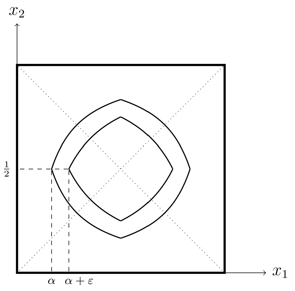
Figure 1. Boundaries of $\mathcal{R}(\alpha)$ and $\mathcal{R}(\alpha+\varepsilon)$ for the uniform distribution in the unit square. Supremum in the definition of $\rho_{H}\bigl{(}\mathcal{R}(\alpha),\mathcal{R}(\alpha+\varepsilon)\bigr{)}$ is attained on diagonals.

It can be easily checked that the supremum in the definition of $\rho_{H}\bigl{(}\mathcal{R}(\alpha),\mathcal{R}(\alpha+\varepsilon)\bigr{)}$ is attained on the diagonals $x_{1}=x_{2}$ and $x_{1}+x_{2}=1$. Note that, in a small neighbourhood $K_{0}$ of $\bigl{(}\sqrt{\frac{\alpha}{2}},\sqrt{\frac{\alpha}{2}}\bigr{)}$, which is the intersection point of $\partial\mathcal{R}(\alpha)$ and $x_{1}=x_{2}$, conditions (C3) and (C4) hold. Hence, Remark  5.6 applies with

$$\min_{x\in\partial\mathcal{R}(\alpha)\cap K_{0}}T_{x,u_{x}}\mu=2\sqrt{\alpha},$$

being the length of the segment tangent to $\partial\mathcal{R}(\alpha)$ at the point $\bigl{(}\sqrt{\frac{\alpha}{2}},\sqrt{\frac{\alpha}{2}}\bigr{)}$. Therefore, Theorem 6.3 holds for $\alpha\in(0,1/2)$ with $\limsup$ given by $\frac{1}{2}\sqrt{M-\alpha}$. The same approach can be applied for any uniform distribution $\mu$ on a polygon, since, in this case, $\partial\mathcal{R}(\alpha)$ consists of a finite number of hyperbolic arcs, see Sections 5.3-5.5 in [18].

Example 7.4 (Normal distribution).

Let $\mu$ be the standard bivariate normal distribution in $\mathbb{R}^{2}$. Due to spherical symmetry of $\mu$, we have $D(x)=\frac{1}{2}-\Phi_{0}\bigl{(}\|x\|\bigr{)}$, $x\in\mathbb{R}^{2}$, where

$$\Phi_{0}(t)=\frac{1}{\sqrt{2\pi}}\int_{0}^{t}\mathrm{e}^{-s^{2}/2}\,\mathrm{d}s.$$

Hence,

$$\mathcal{R}(\alpha)=\bigl{\{}x\in\mathbb{R}^{2}\colon\|x\|\leq\Phi_{0}^{\leftarrow}(1/2-\alpha)\bigr{\}},\quad\alpha\leq 1/2,$$

is the centred disk with radius given by the inverse of $\Phi_{0}$, see also Section 5.7 in [18]. For $\alpha\in(0,1/2)$ and $x\in\partial\mathcal{R}(\alpha)$, we have

$$T_{x,u_{x}}\mu=\biggl{.}\frac{1}{2\pi}\int_{-\infty}^{\infty}\mathrm{e}^{-\frac{1}{2}(s^{2}+t^{2})}\,\mathrm{d}t\,\biggr{|}_{s=\Phi_{0}^{\leftarrow}(1/2-\alpha)}=\frac{1}{\sqrt{2\pi}}\mathrm{e}^{-\frac{1}{2}(\Phi_{0}^{\leftarrow}(1/2-\alpha))^{2}}.$$

Therefore, Theorem 6.3 holds for $\alpha\in(0,1/2)$ with the right-hand side of (6.2) being

$$\sqrt{2\pi(M\alpha-\alpha^{2})}\;\mathrm{e}^{\frac{1}{2}(\Phi_{0}^{\leftarrow}(1/2-\alpha))^{2}}.$$

Example 7.5 (Cauchy distribution).

Let $\mu$ be the bivariate Cauchy distribution with the density

$$f(x)=\frac{1}{\pi^{2}}\frac{1}{(1+x_{1}^{2})(1+x_{2}^{2})},\qquad x=(x_{1},x_{2})\in\mathbb{R}^{2}.$$

Due to Section 5.8 in [18],

$$D(x)=\frac{1}{2}-\frac{1}{\pi}\arctan\max\bigl{\{}|x_{1}|,|x_{2}|\bigr{\}},\qquad x\in\mathbb{R}^{2},$$

$$\mathcal{R}(\alpha)=\bigl{\{}x\in\mathbb{R}^{2}\colon\max\{|x_{1}|,|x_{2}|\}\leq\cot\pi\alpha\bigr{\}},\qquad\alpha\leq 1/2,$$

which is the square with vertices $(\pm\cot\pi\alpha,\pm\cot\pi\alpha)$. The Hausdorff distance $\rho_{H}\bigl{(}\mathcal{R}(\alpha),\mathcal{R}(\alpha+\varepsilon)\bigr{)}$ equals the distance between the vertices of the corresponding squares, where the depth function $D$ is not differentiable. Hence, Theorem 6.3 is not applicable even with Remark 5.6 taken into account. However, these vertices are located on fixed diagonals $x_{1}\pm x_{2}=0$, and so the Hausdorff distance can be calculated explicitly as

$$\rho_{H}\bigl{(}\mathcal{R}(\alpha),\mathcal{R}(\alpha+\varepsilon)\bigr{)}=\sqrt{2}\,\bigl{|}\cot\pi(\alpha+\varepsilon)-\cot\pi\alpha\bigr{|}.$$ (7.1)

Then (6.3) and (7.1) yield

$$\rho_{H}\bigl{(}\mathcal{R}(\alpha),\widehat{\mathcal{R}}_{n}(\alpha)\bigr{)}\leq\sqrt{2}\max\bigl{\{}\cot\pi(\alpha-\gamma\lambda_{n})-\cot\pi\alpha,\cot\pi\alpha-\cot\pi(\alpha+\gamma\lambda_{n})\bigr{\}}\\ =\frac{\pi\sqrt{2}\,\gamma\lambda_{n}}{\sin^{2}\pi\alpha}+o(\lambda_{n})\quad\text{as}\;n\to\infty,$$

for any $\gamma>\sqrt{M\alpha-\alpha^{2}}$. Hence,

$$\limsup_{n\to\infty}\lambda_{n}^{-1}\rho_{H}\bigl{(}\mathcal{R}(\alpha),\widehat{\mathcal{R}}_{n}(\alpha)\bigr{)}\leq\frac{\pi\sqrt{2(M\alpha-\alpha^{2})}}{\sin^{2}\pi\alpha}.$$

To prove the reverse inequality, we can not directly follow the approach used in the proof of Theorem 6.3 since a minimal halfspace at a vertex of $\partial\mathcal{R}(\alpha)$ is not unique. But, with some loss of optimality, we can apply the same technique to any point $x$ of the boundary which is not a vertex. In this case,

$$T_{x,u_{x}}\mu=\biggl{.}\frac{1}{\pi^{2}}\int_{-\infty}^{\infty}\frac{1}{(1+s^{2})(1+t^{2})}\,\mathrm{d}t\,\biggr{|}_{s=\cot\pi\alpha}=\frac{\sin^{2}\pi\alpha}{\pi},$$

which results in the lower bound

$$\frac{\pi\sqrt{M\alpha-\alpha^{2}}}{\sin^{2}\pi\alpha}.$$

Therefore, Theorem 6.3 holds for $\alpha\in(0,1/2)$ with (6.2) replaced by the inequality

$$\frac{\pi\sqrt{M\alpha-\alpha^{2}}}{\sin^{2}\pi\alpha}\leq\limsup_{n\to\infty}\lambda_{n}^{-1}\rho_{H}\bigl{(}\mathcal{R}(\alpha),\widehat{\mathcal{R}}_{n}(\alpha)\bigr{)}\leq\frac{\pi\sqrt{2(M\alpha-\alpha^{2})}}{\sin^{2}\pi\alpha}.$$

The same approach applies to further symmetric distributions, where $\mathcal{R}(\alpha)$ is also a square, see Example 2 in [17].

8. Appendix: Depth functions of convex bodies

Consider a convex body $K$ in $\mathbb{R}^{d}$, and let $\mu$ be the uniform probability distribution on $K$, that is, $\mu$ is the Lebesgue measure on $K$ normalised by the volume $V_{d}(K)$ of $K$. By rescaling, in all subsequent arguments it is possible to let $V_{d}(K)=1$. The depth trimmed region of $\mu$ at level $\alpha$ is said to be the convex floating body $K_{\alpha}$ of $K$, see [20]. Then

$$D(x)=\sup\{\alpha\colon x\in K_{\alpha}\},\quad x\in K,$$

is the depth function of $\mu$.

For a convex set $L$ in $\mathbb{R}^{d}$ denote by $C(L)$ its centroid, that is,

$$C(L)=\frac{1}{V_{j}(L)}\int_{L}x\,\mathrm{d}x,$$

where $j$ is the dimension of $L$, the integral is understood with respect to the Lebesgue measure on the affine subspace generated by $L$, and the normalising factor is the $j$-dimensional Lebesgue measure of $L$.

For a set $L$ and $r>0$ denote by

$$L^{r}=\{x\in\mathbb{R}^{d}\colon\rho(x,L)\leq r\}\quad\text{ and }\quad L^{-r}=\{x\in\mathbb{R}^{d}\colon B_{r}(x)\subset L\}$$

the outer and inner $r$-envelopes of $L$. If $L$ is a convex set, then the Steiner formula says

$$V_{d}(L^{r})=\sum_{i=0}^{d}r^{d-i}\kappa_{d-i}V_{i}(L),$$

where $V_{i}(L)$, $i=0,\dots,d$, are intrinsic volumes of $L$ and $\kappa_{j}$ is the volume of the unit Euclidean ball in $\mathbb{R}^{j}$, see [19, Section 4.1]. Furthermore, denote $\|L\|=\sup\{\|x\|\colon x\in L\}$ and

$$m(L)=\sum_{i=0}^{d}\kappa_{d-i}V_{i}(L).$$

If $E$ is a linear subspace of $\mathbb{R}^{d}$, denote by $\operatorname{proj}_{E}x$ the orthogonal projection of $x$ onto $E$. For each $w,v\in\SS^{d-1}$, denote by $w_{v}$ the normalised projection of $w$ on $\partial H_{v}$.

Lemma 8.1.

Assume that $K$ is a convex body in $\mathbb{R}^{d}$, and let $\delta>0$ be such that $K^{-\delta}$ is not empty. For each pair of $(d-1)$-dimensional affine hyperplanes $E_{1}$ and $E_{2}$ which intersect $K^{-\delta}$, we have that

$$\rho_{H}(K\cap E_{1},K\cap E_{2})\leq c_{1}\rho_{H}(E_{1},E_{2})$$

and

$$\|C(K\cap E_{1})-C(K\cap E_{2})\|\leq c_{2}\rho_{H}(E_{1},E_{2})$$

with constants $c_{1}$ and $c_{2}$ depending only on $K$ and $\delta$.

Proof.

It suffices to consider only parallel $E_{1}$ and $E_{2}$ since otherwise the Hausdorff distance between them is infinite. Denote $\varepsilon=\rho_{H}(E_{1},E_{2})$. Let $u$ be the unit normal to $E_{1}$ such that $E_{2}=E_{1}+\varepsilon u$. Furthermore, let $x$ be any support point of $K$ in direction $u$, that is, $h(K,u)=\langle x,u\rangle$, and let $M$ be the convex hull of $x$ and $K\cap E_{1}$. Since $E_{1}$ intersects $K^{-\delta}$, the distance between $x$ and $E_{1}$ is at least $\delta$, so that $M$ is a cone of height at least $\delta$. Then

$$K\cap E_{1}\subset(M\cap E_{2})^{2\delta^{-1}\|K\|\varepsilon}\subset(K\cap E_{2})^{2\delta^{-1}\|K\|\varepsilon}.$$

The same argument with the roles of $E_{1}$ and $E_{2}$ interchanged and with $x$ being the support point in direction $(-u)$ yields the result for the Hausdorff distance with $c_{1}=2\delta^{-1}\|K\|$.

By assumption, we have that $V_{d-1}(K\cap E_{i})\geq\delta^{d-1}\kappa_{d-1}$, $i=1,2$. For all $r\leq 1$,

$$V_{d-1}((K\cap E_{i})^{r})-V_{d-1}(K\cap E_{i}))\leq rm(K\cap E_{i})\leq rm(K),\quad i=1,2,$$

where we used the monotonicity of intrinsic volumes. Without loss of generality, we may assume that $c_{1}\varepsilon\leq 1$. Then, due to the first part of the lemma,

$$|V_{d-1}(K\cap E_{1})-V_{d-1}(K\cap E_{2})|\leq c_{1}\varepsilon m(K).$$

Denote $L=(K\cap E_{2})-\varepsilon u$, where the translation ensures that $L\subset E_{1}$. Thus,

$$\|C (K\cap E_{1})-C(K\cap E_{2})\|$$

$$\leq\frac{1}{V_{d-1}(K\cap E_{1})}\Big{\|}\int_{K\cap E_{1}}x\,\mathrm{d}x-\int_{L}(x+\varepsilon u)\,\mathrm{d}x\Big{\|}$$

$$\qquad\qquad\qquad\qquad\qquad\qquad+\frac{|V_{d-1}(K\cap E_{1})-V_{d-1}(K\cap E_{2})|}{V_{d-1}(K\cap E_{1})V_{d-1}(K\cap E_{2})}\Big{\|}\int_{K\cap E_{2}}x\,\mathrm{d}x\Big{\|}$$

$$\leq\frac{1}{\delta^{d-1}\kappa_{d-1}}\Big{(}\int_{(K\cap E_{1})\Delta L}\|x\|\,\mathrm{d}x\Big{)}+\frac{1}{\delta^{d-1}\kappa_{d-1}}\Big{(}\int_{L}\varepsilon\,\mathrm{d}x+c_{1}\varepsilon m(K)\|C(K\cap E_{2})\|\Big{)}$$

$$\leq\frac{1}{\delta^{d-1}\kappa_{d-1}}\Big{(}2c_{1}\varepsilon m(K)\|K\|+\varepsilon m(K)(c_{1}\|K\|+1)\Big{)}=c_{2}\varepsilon,$$

where $c_{2}$ depends only on $K$ and $\delta$. ∎

The following result for $K$ with $C^{1}$-boundary can be recovered from the proof of Lemma 5 in [21], however, without a uniform bound on the Lipschitz constant. Recall that $u_{y}$ denotes a unit normal vector to the convex floating body $K_{\alpha}$ at the point $y$ on its boundary.

Lemma 8.2.

Let $K$ be a convex body in $\mathbb{R}^{d}$, and let $\delta>0$ be such that $K^{-\delta}$ is not empty. Then

$$\mu(y+H_{v})-\mu(y+H_{u_{y}})\leq c\|v-u_{y}\|^{2},\quad y\in K^{-\delta},$$

for a constant $c$ which depends only on $\delta$ and $K$.

Proof.

Applying a translation, assume that $y=0$ and denote $u=u_{y}$. Let $L=K\cap\partial H_{u}$. Furthermore, let $L_{1}$ be the set of $x\in L$ such that $\operatorname{proj}_{\partial H_{v}}x\in K$, and let $L_{2}$ be the set of all $x\in\partial H_{u}$ such that the segment which joins $x$ and $y=\operatorname{proj}_{\partial H_{v}}x$ intersects $K$. Note that $L_{1}\subset L\subset L_{2}$.

In the following we use the inequality

$$\|z-\operatorname{proj}_{\partial H_{v}}z\|=|\langle z,v\rangle|=|\langle z,v-u\rangle|\leq\|z\|\|v-u\|,\quad z\in\partial H_{u}.$$

Denote by $r_{M}(w)$ the radial function of a convex set $M$ in direction $w\in\SS^{d-1}$.

Consider $w\in\SS^{d-1}\cap\partial H_{u}$ and $z=r_{L_{2}}(w)w$, which belongs to the relative boundary of $L_{2}$. Let $y$ belong to the intersection of $K$ and the segment which joins $z$ and $z_{1}=\operatorname{proj}_{\partial H_{v}}z$. Then $y$ belongs to the boundary of $K$ and the line passing through $z$ and $z_{1}$ is a tangent line to $K$, so that $y$ belongs to $\partial H_{v^{\prime}}$ with $v^{\prime}$ being a convex combination of $u$ and $v$. Then $y=r_{K}(w_{v^{\prime}})w_{v^{\prime}}$. Since $r_{K}(w)=r_{L}(w)$ and $\|y-z\|\leq\|z_{1}-z\|$,

$$|r_{L}(w)-r_{L_{2}}(w)| \leq\|r_{K}(w)w-y\|+\|y-z\|$$

$$\leq\|r_{K}(w)w-r_{K}(w_{v^{\prime}})w\|+\|r_{K}(w_{v^{\prime}})w-r_{K}(w_{v^{\prime}})w_{v^{\prime}}\|+\|\operatorname{proj}_{\partial H_{v^{\prime}}}z-z\|$$

$$\leq|r_{K}(w)-r_{K}(w_{v^{\prime}})|+r_{K}(w_{v^{\prime}})\|w-w_{v^{\prime}}\|+\|z\|\|u-v\|.$$

The radial function $r_{K}$ is Lipschitz, that is, $|r_{K}(w_{v^{\prime}})-r_{K}(w)|\leq c_{3}\|w_{v^{\prime}}-w\|$, with a constant $c_{3}$ depending only on $\delta$ and $K$. This is seen by writing $r_{K}(u)=h(K^{o},u)^{-1}$, using the support function of the polar body to $K$ and noticing that $K^{o}$ is contained in the ball of radius $\delta^{-1}$ and contains the ball of radius $\|K\|^{-1}$ and the fact that the support function is Lipschitz. Note also that $r_{K}(w)$ is bounded by a constant which depends on $K$. Thus, and since $\|w_{v^{\prime}}-w\|\leq\|v^{\prime}-u\|\leq\|v-u\|$, we have

$$|r_{L}(w)-r_{L_{2}}(w)|\leq c_{4}\|v-u\|$$

for all $w\in\SS^{d-1}\cap\partial H_{u}$. Since the Hausdorff distance between convex sets is bounded by the uniform distance between their radial functions, $\rho_{H}(L,L_{2})\leq c_{4}\|u-v\|$.

Now consider the set $L_{1}$, take $w\in\SS^{d-1}\cap\partial H_{u}$, and let $z_{1}=\operatorname{proj}_{\partial H_{v}}z$ for $z=r_{L}(w)w$. If $z_{1}\in K$, then $z$ lies on the boundary of $L_{1}$ and $r_{L_{1}}(w)=r_{L}(w)$. If $z_{1}\notin K$, then the point $z_{2}\in L$ with $r_{K}(w_{v})w_{v}=\operatorname{proj}_{\partial H_{v}}z_{2}$ lies on the boundary of $L_{1}$, so that

$$r_{L}(w)-r_{L_{1}}(w) =\|r_{K}(w)w-z_{2}\|$$

$$\leq\|r_{K}(w)w-r_{K}(w_{v})w_{v}\|+\|r_{K}(w_{v})w_{v}-z_{2}\|$$

$$\leq|r_{K}(w)-r_{K}(w_{v})|+r_{K}(w)\|w-w_{v}\|+\|\operatorname{proj}_{\partial H_{v}}z_{2}-z_{2}\|$$

$$\leq c_{5}\|u-v\|.$$

Arguing as above, we obtain $\rho_{H}(L,L_{1})\leq c_{5}\|v-u\|$. Combining this with the bound on $\rho_{H}(L,L_{2})$ yields that

$$L_{2}\subset L_{1}+c_{6}\|u-v\|B^{d-1},$$ (8.1)

where $B^{d-1}$ is the unit ball in the space $\partial H_{u}$ of dimension $(d-1)$.

Denote

$$M =\{z\in\mathbb{R}^{d}\colon\langle z,u\rangle\langle z,v\rangle\leq 0\},$$

$$h =\sup\{\|z-\operatorname{proj}_{\partial H_{v}}z\|\colon z\in L_{2}\}.$$

Note that $h\leq c_{7}\|u-v\|$. Furthermore, let

$$Z=M\cap\operatorname{conv}(L\cup\operatorname{proj}_{\partial H_{v}}L).$$

Then

$$\mu(H_{v})-\mu(H_{u})\leq|V_{d}(Z\cap H_{v})-V_{d}(Z\cap H_{u})|+V_{d}(M\cap(K\triangle Z)).$$

Note that $M\cap(K\triangle Z)$ is a subset of the difference of two cylinders, $C_{2}=L_{2}+[-hv,hv]$ and $C_{1}=L_{1}+[-hv,hv]$. By (8.1),

$$V_{d}(M\cap(K\triangle Z))\leq V_{d}(C_{2})-V_{d}(C_{1}) =2h\big{(}V_{d-1}(L_{2})-V_{d-1}(L_{1})\big{)}$$

$$=2h\sum_{i=0}^{d-2}(c_{6}\|u-v\|)^{d-1-i}\kappa_{d-1-i}V_{i}(L_{1})\leq c_{8}\|u-v\|^{2}.$$

Finally,

$$V_{d}(Z\cap H_{u})-V_{d}(Z\cap H_{v})=\langle u,v\rangle\int_{z\in L}\langle z,v\rangle\mathrm{d}z=\langle u,v\rangle\Big{\langle}\int_{z\in L}z\mathrm{d}z,v\Big{\rangle}=0,$$

where $\langle u,v\rangle$ is the Jacobian of the linear transformation used in the integral, and the last integral vanishes since $0$ is the centroid of $L=K\cap H_{u}$, see, e.g., [21, Lemma 2]. ∎

A convex body is said to be smooth if each point on its boundary admits a unique outer normal; it is symmetric if $K$ equals its reflection with respect to some point which is usually put at the origin; $K$ is strictly convex if its boundary does not contain any segment. It is known that if $K$ is symmetric smooth and strictly convex, then the convex floating body $K_{\alpha}$ is of the class $C^{2}$ for all $0<\alpha<V_{d}(K)/2=\alpha_{\max}$, see [12, Theorem 3]. Then, each $x\neq 0$ from the interior of $K$ belongs to some $\partial K_{\alpha}$ and there exists a unique outer normal vector $u_{x}$ to $K_{\alpha}$ such that $\mu(x+H_{u_{x}})=\alpha$, see Lemma 2.1.

Lemma 8.3.

Assume that $K$ is a symmetric smooth strictly convex body. Then the function $x\mapsto u_{x}$ is Lipschitz on $\{x\in K\colon\delta_{1}\leq D(x)\leq\delta_{2}\}$, where $0<\delta_{1}<\delta_{2}<V_{d}(K)/2$, and the Lipschitz constant depends on $K$ and $\delta_{1},\delta_{2}$.

Proof.

Assume that $D(x)=t$ and $D(y)=s$, where $\delta_{1}\leq t\leq s\leq\delta_{2}$ without loss of generality.

We first settle the case when $t=s$, so that both $x$ and $y$ belong to the boundary of $K_{t}$ for some $t\in[\delta_{1},\delta_{2}]$. It is known from [9, Eq. (19)] and [21, Lemma 4] that the radius of curvature $R(x)$ of $K_{t}$ at a point $x$ on its boundary equals the determinant of the matrix $Q$ given by

$$Q_{i,j}=\frac{1}{V_{d-1}(K\cap E)}\int_{\mathbb{S}^{d-2}}\eta_{i}\eta_{j}r(\eta)^{d}\cot\beta(\eta)\mathrm{d}\eta,\quad i,j=1,\dots,d-1,$$

where $E$ is the $(d-1)$-dimensional affine space passing through $x$ with normal $u_{x}$, that is, the tangent plane to $K_{t}$ at $x$, the integration is over the unit sphere in $E$, and $r(\eta)$ is the radial function of $K\cap E$. The angle $\beta(\eta)$ is built by the half-line $\ell(\eta)$ through $x$ in direction $\eta\in E$ and the tangent half-line to $\partial K$ at $y=\ell(\eta)\cap\partial K$, whose orthogonal projection onto $E$ is $\ell(\eta)$ and which belongs to the complement of $x+H_{u_{x}}$, see Figure 2 in [12].

The determinant of $Q$ is bounded below by the $(d-1)$th power of the infimum of

$$\frac{1}{V_{d-1}(K\cap E)}\int_{\mathbb{S}^{d-2}}\langle\eta,y\rangle^{2}r(\eta)^{d}\cot\beta(\eta)\mathrm{d}\eta$$

for all $y$ from the unit sphere $\mathbb{S}^{d-2}$ in $E$. As in the proof of [12, Theorem 3], let $\tilde{K}$ be the convex hull of $K\cap E$ and $K\cap(-E)$, and let $\tilde{\beta}(\eta)$ be the maximum of the angles constructed for $\tilde{K}$ in the same way as $\beta(\eta)$ was constructed for $K$. Since $t\leq\delta_{2}<V_{d}(K)/2$ and $K$ is strictly convex,

$$\tilde{\beta}(\eta)\geq\varepsilon+\beta(\eta)$$

for some $\varepsilon>0$, all $\eta\in\mathbb{S}^{d-2}$, and all $x$ with $D(x)\in[\delta_{1},\delta_{2}]$. By Theorem 1 from [12] we have

$$0\leq\int_{\mathbb{S}^{d-2}}\langle\eta,y\rangle^{2}r(\eta)^{d}\cot\tilde{\beta}(\eta)\mathrm{d}\eta\leq\int_{\mathbb{S}^{d-2}}\langle\eta,y\rangle^{2}r(\eta)^{d}\cot\beta(\eta)\mathrm{d}\eta-\varepsilon\int_{\mathbb{S}^{d-2}}\langle\eta,y\rangle^{2}r(\eta)^{d}\mathrm{d}\eta,$$

where we have used the inequality $\cot(\beta)-\cot(\beta+\varepsilon)\geq\varepsilon$. Thus,

$$R(x)\geq\Big{(}c_{9}\frac{\varepsilon}{V_{d-1}(K\cap E)}\Big{)}^{d-1}.$$

The right-hand side is bounded away from zero for all $x$ with $D(x)\in[\delta_{1},\delta_{2}]$. Thus, the curvatures of sets $K_{t}$ with $t\in[\delta_{1},\delta_{2}]$ are bounded by a constant, so that, $\|u_{x}-u_{y}\|\leq c_{10}\|x-y\|$ for a constant $c_{10}$ which depends on $K$ and $\delta_{1},\delta_{2}$.

Assume now that $t<s$. Let $x\in\partial K_{t}$ with $u_{x}$ being the normal to $K_{t}$ at $x$. Let $z$ be the point on $K_{s}$ with the normal $u_{x}$. Since $\langle y,u_{x}\rangle\leq\langle z,u_{x}\rangle=h(K_{s},u_{x})$, we have that

$$h(K_{t},u_{x})-h(K_{s},u_{x})\leq\|x-y\|.$$

Since $x$ and $z$ are the centroids of the sections $K\cap(x+\partial H_{u_{x}})$ and $K\cap(z+\partial H_{u_{x}})$, respectively, and $K_{t}$ is a subset of $K^{-\delta}$ for some $\delta>0$, Lemma 8.1 yields that $\|x-z\|\leq c_{2}\|x-y\|$. Hence, $\|z-y\|\leq c_{11}\|x-y\|$, and, by the boundedness of curvatures of convex floating bodies, we have that $\|u_{x}-u_{y}\|=\|u_{z}-u_{y}\|\leq c_{12}\|x-y\|$. ∎

Theorem 8.4.

Assume that $\mu$ is the uniform distribution on a centrally symmetric smooth strictly convex body $K$. Then the depth function is continuously differentiable on the interior of $K$ and

$$\operatorname{grad}D(x)=\frac{V_{d-1}(K\cap(x+\partial H_{u_{x}}))}{V_{d}(K)}.$$

Proof.

The proof follows the argument from the proof of Lemma 5.2. Namely,

$$D(x)-D(y)=\mu(x+H_{u_{x}})-\mu(y+H_{u_{y}})=\Big{(}\mu(x+H_{u_{x}})-\mu(y+H_{u_{x}})\Big{)}+\Big{(}\mu(y+H_{u_{x}})-\mu(y+H_{u_{y}})\Big{)}.$$

The first term is continuously differentiable, and the second one is of the order $\|x-y\|^{2}$ uniformly in $x$ due to Lemmas 8.2 and 8.3. ∎

References

- [1] K. S. Alexander and M. Talagrand. The law of the iterated logarithm for empirical processes on Vapnik-Červonenkis classes. J. Multivariate Anal., 30:155 – 166, 1989.
- [2] I. Bárány. Intrinsic volumes and -vectors of random polytopes. Math. Ann., 285(4):671–699, 1989.
- [3] A. A. Borovkov. Mathematical Statistics. Gordon and Breach Science Publishers, Amsterdam, 1998.
- [4] V.-E. Brunel. Concentration of the empirical level sets of Tukey’s halfspace depth. Probab. Theory Related Fields, 173:1165–1196, 2019.
- [5] M. Csörgő and P. Révész. Strong approximations of the quantile process. Ann. Statist., 6(4):882–894, 1978.
- [6] K. Dutta, A. Ghosh, and S. Moran. Uniform Brackets, Containers, and Combinatorial Macbeath Regions. In 13th Innovations in Theoretical Computer Science Conference (ITCS 2022), volume 215 of Leibniz International Proceedings in Informatics (LIPIcs), pages 59:1–59:10, Dagstuhl, Germany, 2022.
- [7] R. Dyckerhoff. Convergence of depths and depth-trimmed regions. Technical report, arXiv math:1611.08721, 2017.
- [8] A. Ilienko and I. Molchanov. Limit theorems for multidimensional renewal sets. Acta Math. Hungar., 156(1):56–81, 2018.
- [9] K. Leichtweiss. Über eine Formel Blaschkes zur Affinoberfläche. Studia Sci. Math. Hungar., 21(3-4):453–474, 1986.
- [10] P. Massart and E. Rio. A uniform Marcinkiewicz-Zygmund strong law of large numbers for empirical processes. In Asymptotic Methods in Probability and Statistics (Ottawa, ON, 1997), pages 199–211. North-Holland, Amsterdam, 1998.
- [11] J.-C. Massé. Asymptotics for the Tukey depth process, with an application to the multivariate trimmed mean. Bernoulli, 10:397–420, 2004.
- [12] M. Meyer and S. Reisner. A geometric property of the boundary of symmetric convex bodies and convexity of flotation surfaces. Geometriae Dedicata, 37:327–337, 01 1991.
- [13] I. Mizera and M. Volauf. Continuity of halfspace depth contours and maximum depth estimators: diagnostics of depth-related methods. J. Multivariate Anal., 83(2):365–388, 2002.
- [14] I. Molchanov. A limit theorem for solutions of inequalities. Scand. J. Statist., 25(1):235–242, 1998.
- [15] I. Molchanov. Theory of Random Sets. London: Springer, 2nd edition, 2017.
- [16] M. Molina-Fructuoso and R. Murray. Tukey depths and Hamilton-Jacobi differential equations. SIAM J. Math. Data Sci., 4(2):604–633, 2022.
- [17] S. Nagy, C. Schütt, and E. M. Werner. Halfspace depth and floating body. Stat. Surv., 13:52–118, 2019.
- [18] P. J. Rousseeuw and I. Ruts. The depth function of a population distribution. Metrika, 49:213–244, 1999.
- [19] R. Schneider. Convex Bodies. The Brunn–Minkowski Theory. Cambridge University Press, Cambridge, 2nd edition, 2014.
- [20] C. Schütt and E. Werner. The convex floating body. Math. Scand., 66:275–290, 1990.
- [21] C. Schütt and E. Werner. Homothetic floating bodies. Geom. Dedicata, 49(3):335–348, 1994.
- [22] G. R. Shorack and J. A. Wellner. Empirical Processes with Applications to Statistics. John Wiley & Sons, Inc., New York, 1986.
- [23] J. W. Tukey. Mathematics and the picturing of data. In Proceedings of the International Congress of Mathematicians (Vancouver, B. C., 1974), Vol. 2, pages 523–531, 1975.
- [24] A. W. van der Vaart and J. A. Wellner. Weak Convergence and Empirical Processes. Springer-Verlag, New York, 1996.