A Simple Framework for Multi-mode Spatial-Temporal Data Modeling

Abstract

Spatial-temporal data modeling aims to mine the underlying spatial relationships and temporal dependencies of objects in a system. However, most existing methods focus on the modeling of spatial-temporal data in a single mode, lacking the understanding of multiple modes. Though very few methods have been presented to learn the multi-mode relationships recently, they are built on complicated components with higher model complexities. In this paper, we propose a simple framework for multi-mode spatial-temporal data modeling to bring both effectiveness and efficiency together. Specifically, we design a general cross-mode spatial relationships learning component to adaptively establish connections between multiple modes and propagate information along the learned connections. Moreover, we employ multi-layer perceptrons to capture the temporal dependencies and channel correlations, which are conceptually and technically succinct. Experiments on three real-world datasets show that our model can consistently outperform the baselines with lower space and time complexity, opening up a promising direction for modeling spatial-temporal data. The generalizability of the cross-mode spatial relationships learning module is also validated. Codes and datasets are available at https://github.com/lzhmarkk/SimMST.

I Introduction

Spatial-temporal data record the information of objects across both space and time in a system, which are pervasive in many applications, such as traffic forecasting [1, 2], air quality inference [3, 4], and electricity consumption prediction [5, 6]. In recent years, spatial-temporal modeling has attracted a lot of attention, whose core is to mine the underlying spatial relationships and temporal dependencies of objects [7, 8].

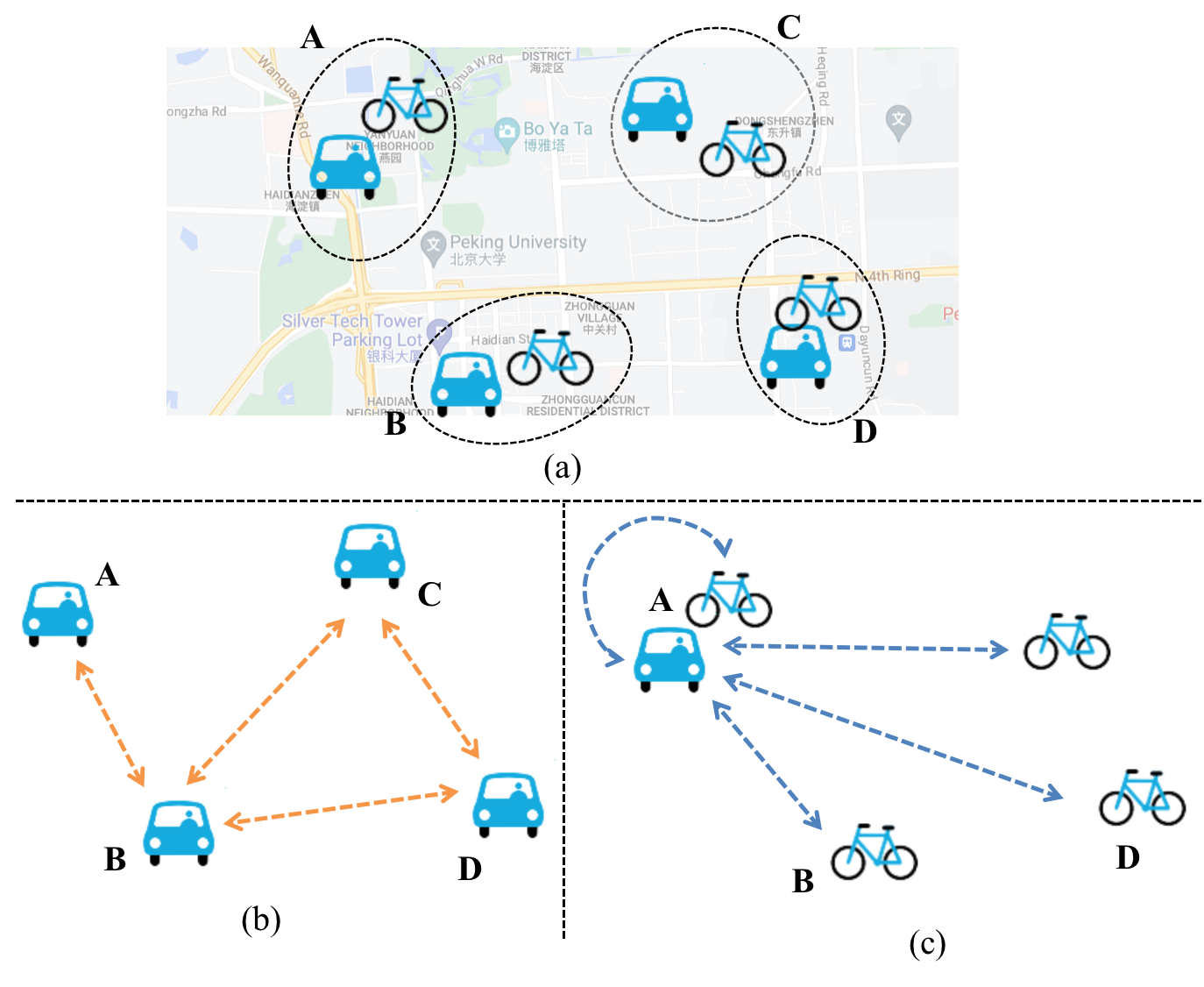
Figure 1: Illustrations of spatial and mode dependency of multi-mode spatial-temporal data. (a) Multiple modes of a specific location can be simultaneously observed in many real-world scenarios, e.g. bike and taxi demands of each location. (b) Most previous works consider the spatial relationships between locations with only a single mode. (c) The correlations between different modes remain to be investigated.

Existing methods for spatial-temporal data modeling mainly learn from a single mode [1, 2, 3, 7, 9, 4, 10, 11, 5, 12, 6, 13]. For example, [2] combined the Graph Neural Networks (GNNs) [14] and convolutional sequence learning modules to jointly extract spatial-temporal features for traffic speed forecasting. [5] designed a GNN-based framework to exploit the inherent relationships of different single-mode sequences. [12] extended [15] with a graph gate for spatial modeling and a time gate to capture multiplicative seasonality. However, in real-world scenarios, multiple factors of a specific location can be simultaneously observed (i.e., multi-mode) and tend to affect each other. For example, the demands of taxis and bikes both exist in one certain area and the changes in taxi demands are often influenced by the variations in bike demands [16, 17]. Therefore, it is essential to investigate the relationships between multiple modes, which cannot be captured by previous methods. Figure 1 demonstrates the spatial and mode dependency of multi-mode spatial-temporal data.

TABLE I: Comparison of components, time complexity and space complexity of single-mode and multi-mode methods. $N$, $T$, $L$, $C$ and $K$ respectively refers to the number of objects, timestamps, layers, features and GCN hops. Other stands for other components such as embedding layers and normalization layers. For fair comparison, we ignore the number of modes $M$ here.

Methods	Multi mode	Spatial					Temporal			Other
		Learning		Propagation
		Time	Space	Component	Time	Space	Component	Time	Space	Time	Space
STGCN	$\times$	-	-	GCN	$\mathcal{O}\left(N^{2}TLK\right)$	$\mathcal{O}\left(LK\right)$	TCN	$\mathcal{O}\left(NTL\right)$	$\mathcal{O}\left(L\right)$	$\mathcal{O}\left(NT(L+C)\right)$	$\mathcal{O}\left(NL+C\right)$
GWNet	$\times$	$\mathcal{O}\left(N^{2}\right)$	$\mathcal{O}\left(N\right)$	GCN	$\mathcal{O}\left(N^{2}TLK\right)$	$\mathcal{O}\left(LK\right)$	TCN	$\mathcal{O}\left(NTL\right)$	$\mathcal{O}\left(L\right)$	$\mathcal{O}\left(NT(L+C)\right)$	$\mathcal{O}\left(L+C\right)$
MTGNN	$\times$	$\mathcal{O}\left(N^{2}\right)$	$\mathcal{O}\left(N\right)$	GCN	$\mathcal{O}\left(N^{2}TLK\right)$	$\mathcal{O}\left(LK\right)$	TCN	$\mathcal{O}\left(NTL\right)$	$\mathcal{O}\left(L\right)$	$\mathcal{O}\left(NT(L+C)\right)$	$\mathcal{O}\left(NTL+C\right)$
ESG	$\times$	$\mathcal{O}\left(N^{2}T\right)$	$\mathcal{O}\left(N+T\right)$	GCN	$\mathcal{O}\left(N^{2}TLK\right)$	$\mathcal{O}\left(LK\right)$	TCN	$\mathcal{O}\left(NTL\right)$	$\mathcal{O}\left(L\right)$	$\mathcal{O}\left(NT(L+C)\right)$	$\mathcal{O}\left(NTL+C\right)$
FC-GAGA	$\times$	$\mathcal{O}\left(N^{2}\right)$	$\mathcal{O}\left(N\right)$	MLP	$\mathcal{O}\left(N^{2}TL\right)$	-	MLP	$\mathcal{O}\left(N^{2}TL\right)$	$\mathcal{O}\left(NTL\right)$	$\mathcal{O}\left(NT(L+C)\right)$	$\mathcal{O}\left(TL+C\right)$
MTS-Mixer	$\times$	$\mathcal{O}\left(N^{2}\right)$	$\mathcal{O}\left(N^{2}\right)$	MLP	$\mathcal{O}\left(N^{2}TC\right)$	-	MLP	$\mathcal{O}\left(NT^{2}C\right)$	$\mathcal{O}\left(T^{2}\right)$	$\mathcal{O}\left(NTLC\right)$	$\mathcal{O}\left(NL\right)$
MOHER	✓	-	-	GCN	$\mathcal{O}\left(N^{2}TK\right)$	$\mathcal{O}\left(K\right)$	LSTM	$\mathcal{O}\left(NT\right)$	$\mathcal{O}\left(1\right)$	$\mathcal{O}\left(NT(L+C)\right)$	$\mathcal{O}\left(C\right)$
CoGNN	✓	$\mathcal{O}\left(N^{2}\right)$	$\mathcal{O}\left(N\right)$	GCN	$\mathcal{O}\left(N^{2}TLK\right)$	$\mathcal{O}\left(LK\right)$	TCN	$\mathcal{O}\left(NTL\right)$	$\mathcal{O}\left(L\right)$	$\mathcal{O}\left(NT(L+C)\right)$	$\mathcal{O}\left(NTL+C\right)$
SimMST	✓	$\mathcal{O}\left(N^{2}\right)$	$\mathcal{O}\left(N\right)$	MLP	$\mathcal{O}\left(N^{2}T\right)$	-	MLP	$\mathcal{O}\left(NT^{2}\right)$	$\mathcal{O}\left(T^{2}\right)$	$\mathcal{O}\left(NTC\right)$	$\mathcal{O}\left(T+C\right)$

In recent years, very few efforts have been made on modeling multi-mode spatial-temporal data. One part of the methods restricted their studied objects to be organized in regular grids in the space, and thus reduced its usability in scenarios with irregular regions [18, 19, 16, 20]. Other methods tried to apply GNNs to break the constraints of grids. For instance, MOHER [21] and CoGNN [17] utilized GNNs to propagate information along the connections between nodes and modes to explore multiple modes’ relationships. Although insightful, they are built on complicated modules, which inevitably introduce more learnable parameters and incur higher computational costs. We provide the analysis of existing methods in Table I, which shows that they either fail to capture multi-mode relationships or require complex components. Specifically, most methods use Temporal Convolutional Networks (TCNs) to learn temporal dependencies. They concatenate multiple filters with different kernel sizes to capture temporal patterns with different granularities and use dilation configurations for larger receptive fields. Moreover, these methods stack multiple GNN layers to propagate high-order spatial information. ESG [6] even entangles recurrent modules with graph structure learning. These complex designs are computationally expensive but might not be necessary.

To this end, we aim to investigate whether it is necessary to design sophisticated components for modeling multi-mode spatial-temporal data. To be specific, we propose a Simple framework for Multi-mode Spatial-Temporal data modeling (SimMST) to bring both effectiveness and efficiency together. A general cross-mode spatial relationships learning component is designed, which can adaptively establish connections between multiple modes and propagate information along the learned connections. Also, we leverage multi-layer perceptrons to capture the temporal dependencies and channel correlations. Our approach is built by stacking the above components multiple times and can be trained in an end-to-end manner. We conduct extensive experiments on three real-world datasets, and the results demonstrate that our model outperforms existing methods with fewer learnable parameters and lower computational costs. We also integrate the proposed cross-mode spatial relationships learning module into existing methods and find that this module is general and can bring improvements due to the learning of multi-mode relationships. Our main contributions include:

• We are the first to show the task of multi-mode spatial-temporal data modeling can be well tackled by a simple framework, which can simultaneously learn the temporal dependencies, cross-mode spatial relationships, and channel correlations.

• A cross-mode spatial relationships learning component is designed, which can adaptively learn connections between different modes and propagate information along the connections. This module is general and applicable to existing spatial-temporal modeling methods.

• Extensive experimental results show the superiority of our approach over existing methods, which motivates future research to rethink the key factors for modeling multi-mode spatial-temporal data as well as the potential of simple architectures.

II Preliminaries

TABLE II: Some important notations used in this paper.

Notation	Implication
$\mathbb{M}$	The set of all modes (e.g. railway, bus)
$\mathbb{N}$	The set of all objects (e.g. regions)
$M$	Total number of modes
$N$	Total number of objects
$T$	Total number of timestamps
$C$	Total number of features
$L$	Total number of model layers
$m$	A mode
$n$	An object
$t$	A timestamp
$c$	A feature
$\mathbf{A}_{m_{i},m_{j}}$	Relationship matrix between modes $m_{i}$ and $m_{j}$
$\mathbf{H^{l}}$	Hidden state of layer $l$
$\mathbf{X}$	Input history observations
$\mathbf{\hat{Y}}$	Output predicted observations
$\mathbf{X}_{m}$	Input history observations with mode $m$
$\mathbf{\hat{Y}}_{m}$	Output predicted observations with mode $m$

II-A Multi-mode Spatial-Temporal Data

Let $\mathbb{N}=\{n_{1},\cdots,n_{N}\}$ denote the set of all the studied objects with $N$ as the cardinality. Let $\mathbb{M}=\{m_{1},\cdots,m_{M}\}$ represents the set of all the modes with $M$ as the cardinality. We denote observations of object $n\in\mathbb{N}$ with mode $m\in\mathbb{M}$ at time $t$ by $\bm{X}_{m,n,t,*}\in\mathbb{R}^{C}$, where $C$ is the feature dimension and $*$ refers to all entities in the corresponding dimension. Therefore, the observations of all objects with mode $m$ at all timestamps can be denoted as $\bm{X}_{m,*,*,*}\in\mathbb{R}^{N\times T\times C}$, where $T$ is the total number of timestamps. By stacking $M$ modes, we can represent the multi-mode spatial-temporal data as $\bm{X}\in\mathbb{R}^{M\times N\times T\times C}$. Take the traffic forecasting task as an example, each region has observations with several traffic modes at different times, such as the demand of taxis, bikes, and buses, which could be formalized as multi-mode spatial-temporal data.

II-B Multi-mode Relation Matrices

A multi-mode relation matrix captures the relationships between different objects with two specific modes. Formally, we use matrix $\bm{A}_{m_{i},m_{j}}\in\mathbb{R}^{N\times N}$ to record the relationships of $N$ objects with modes $m_{i},m_{j}\in\mathbb{M}$. Therefore, for $M$ modes, we have $M\times M$ matrices that represent the pairwise relationships between all modes, that is, $\mathcal{A}=\{\bm{A}_{m_{i},m_{j}}|m_{i},m_{j}\in\mathbb{M}\}$.

II-C Problem Formulation

In this paper, we formalize the multi-mode spatial-temporal modeling problem as a forecasting task. Given the observations within historical $W$ timestamps $\bm{X}_{*,*,t-W+1:t,*}\in\mathbb{R}^{M\times N\times W\times C}$, we aim to design an algorithm $\mathcal{F}$ to predict future observations in the next $H$ horizons for all the objects with all the modes, i.e., $\hat{\bm{Y}}_{*,*,t+1:t+H,*}\in\mathbb{R}^{M\times N\times H\times C}$, which can be denoted by the following equation,

$$\hat{\bm{Y}}_{*,*,t+1:t+H,*}=\mathcal{F}\left(\bm{X}_{*,*,t-W+1:t,*}\right).$$ (1)

Table II provides an overview of some important notations used in this paper.

III Methodology

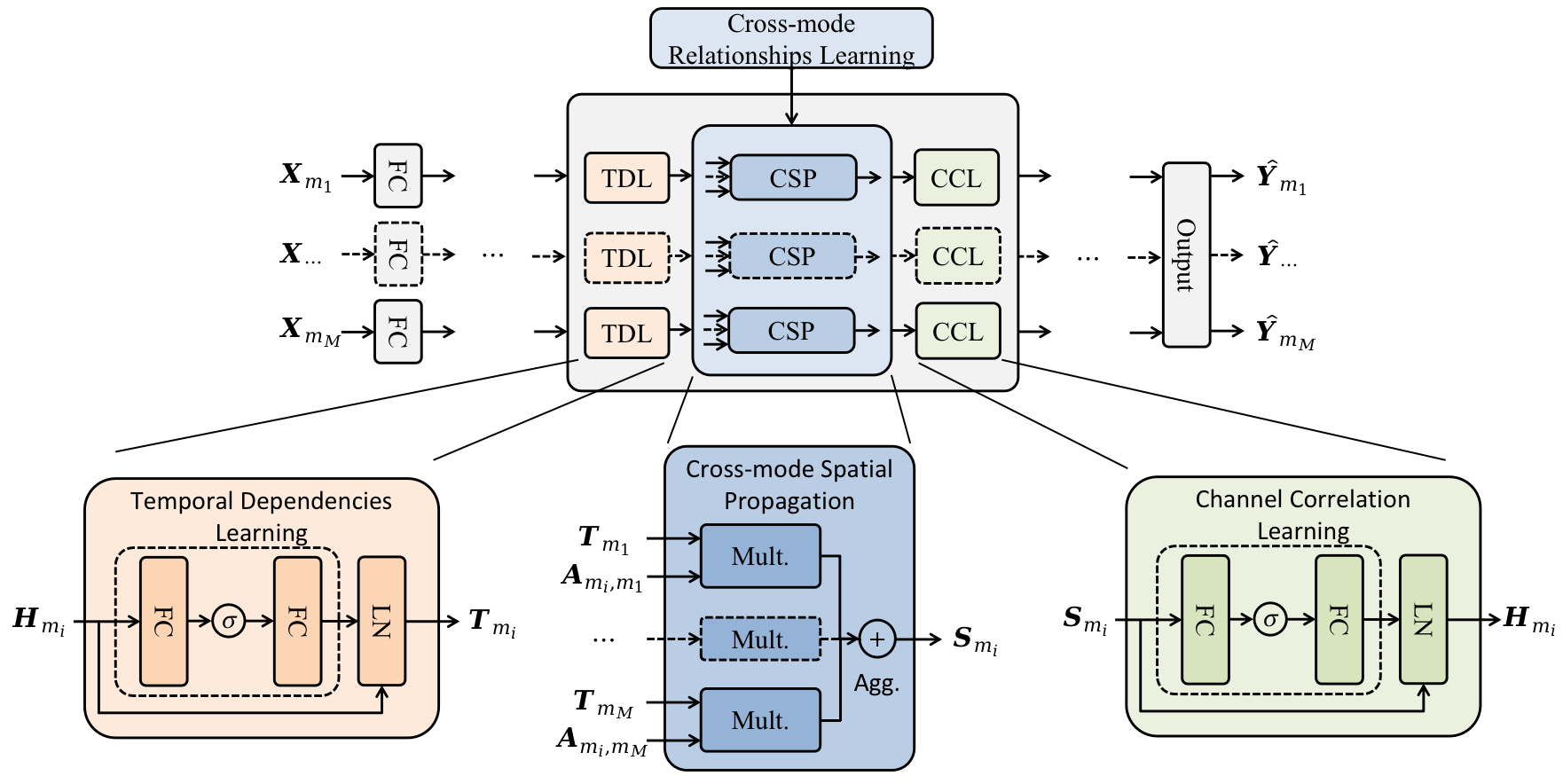
Figure 2: Framework of the proposed SimMST.

In this section, we elaborate on the design of the overall framework and each component.

III-A Overview

Figure 2 presents the framework of our method, which learns from the perspectives of temporal, spatial, cross-mode, and channel. The multi-mode spatial-temporal input $\{\bm{X}_{m_{1}},\bm{X}_{m_{2}},\cdots,\bm{X}_{m_{M}}\}$ is first fed into multiple mode-specific embedding layers $\{f_{1}^{init},f_{2}^{init},\cdots,f_{M}^{init}\}$ to obtain the corresponding initial hidden states $\{\bm{H}_{m_{1}}^{0},\bm{H}_{m_{2}}^{0},\cdots,\bm{H}_{m_{M}}^{0}\}$. Then a Temporal Dependencies Learning (TDL) component is utilized to model temporal evolutionary patterns for each mode, and a Cross-mode Spatial Relationships Learning (CSRL) component is used to capture both spatial relationships and interactions between different modes. Third, a Channel Correlations Learning (CCL) component is employed to learn the correlations of different channels. We stack the above components into layers to obtain hierarchical hidden states and send all hidden states to an output module to generate predictions with each mode.

III-B Temporal Dependencies Learning

Given hidden states of $l-1$ layer $\bm{H}_{m}^{l-1}\in\mathbb{R}^{N\times\ T_{l-1}\times D}$ with time length $T_{l-1}$, Temporal Dependencies Learning (TDL) component models the temporal evolutionary patterns of each object within each mode, which reflect the inherent patterns of each object.

TDL regards the input as time series and conducts information mixing with neural networks $f^{TDL}$ along the temporal dimension. We use a layer normalization operation for regularization and a residual connection to retain the input features. The process of TDL can be denoted as:

$$\bm{T}_{m}^{l}=LN(f^{TDL}_{m}(\bm{H}_{m}^{l-1}))+\bm{H}_{m}^{l-1},$$ (2)

where $f^{TDL}_{m}$ denotes the neural networks applied on the temporal dimension and $m$ refers to mode.

We proposed several forms of empirical configurations of TDL:

1) General configuration. Multi-layer perceptron (MLP) learns the pair-wise influence from each input timestamp to each output timestamp. It has a full receptive field and is naturally sensitive to the input order. Therefore it is suitable to deal with sequences. The length of temporal dimension is reduced by half, which helps to learn high-level temporal information. It can be described with the following equation:

$$f^{TDL}_{m}(\bm{H})=\sigma(\bm{H}\bm{W}_{m,0}^{t,l}+\bm{b}_{m,0}^{t,l})\bm{W}_{m,1}^{t,l}+\bm{b}_{m,1}^{t,l},$$ (3)

where the activation function $\sigma(\cdot)$ is GeLU. $\bm{W}_{m}^{t,l}$ and $\bm{b}_{m}^{t,l}$ are learnable temporal weight and bias parameters.

2) Seasonality configuration. Seasonality describes the recurring and regular characteristics of a series. We adopt Fourier Transforms to discriminate the input into a series of trigonometric functions to better capture the seasonal patterns. It can be described with the following equation:

$$f^{TDL}_{m}(\bm{H})=\mathcal{F}^{-1}\left(\mathcal{F}(\bm{H})\odot\bm{W}_{m}^{t,l}+\bm{b}_{m}^{t,l}\right),$$ (4)

where $\mathcal{F}$ represents FFT operation and $\mathcal{F}^{-1}$ represents inverse FFT operation. $\odot$ refers to Hadamard product.

In this paper, we choose the MLPs as the backbone of TDL. Each timestamp of the output matrix $\bm{T}_{m}^{l}$ receives direct information from all timestamps of the input, and thus the interactions of different timestamps can be learned.

III-C Cross-mode Spatial Relationships Learning

In this component, we aim to model the spatial and multi-mode relationships, which correspond to the $N$ dimension and $M$ dimension of input $\bm{X}$ respectively. The spatial relationships indicate the relations between objects within a mode. For example, the railway demands of an area can be influenced by the railway demands of another area. The multi-mode relationships indicate the impacts between objects with different modes, which are pervasive in real-world scenarios. Intuitively, the railway demand in an area is positively correlated with taxis (the demand brought by the railways will be absorbed by taxis), but the demand for bikes is inversely related to taxis (people either choose bikes or taxis for travel).

In order to explicitly model both spatial and multi-mode relationships, we propose a Cross-mode Spatial Relationships Learning (CSRL) component. It consists of a cross-mode relationships learning module and several cross-mode spatial propagation modules.

Cross-mode Relationships Learning Module. For every two modes $m_{i}$ and $m_{j}$, we use a relation matrix $\bm{A}_{m_{i},m_{j}}$ to record the learned connections from mode $m_{j}$ to mode $m_{i}$. First, we denote the trainable object embeddings with mode $m$ as $\bm{E}_{m}\in\mathbb{R}^{N\times D_{emb}}$, where $D_{emb}$ is the embedding dimension. Then, two MLPs are respectively utilized to retrieve the in-affect embeddings $\bm{E}_{m}^{in}$ and out-affect embeddings $\bm{E}_{m}^{out}$. The relation matrix between mode $m_{j}$ and $m_{i}$ can be denoted as:

$$\tilde{\bm{A}}_{m_{i},m_{j}}=\psi\left(\tau(\bm{E}_{m_{j}}^{out}\times(\bm{E}_{m_{i}}^{in})^{T}-\bm{E}_{m_{j}}^{in}\times(\bm{E}_{m_{i}}^{out})^{T})\right),$$ (5)

where $(\cdot)^{T}$ refers to matrix transposition. The former term in Equation 5 represents the gross impact from mode $m_{j}$ to $m_{i}$, and the latter represents the reverse impact. We can obtain the net impact from mode $m_{j}$ to $m_{i}$ with a subtraction. $\psi(\cdot)$ and $\tau(\cdot)$ are respectively ReLU and Tanh activation functions. We further facilitate the training with self-loops and normalization:

$$\bm{A}_{m_{i},m_{j}}=\bm{D}_{m_{i},m_{j}}^{-1}(\tilde{\bm{A}}_{m_{i},m_{j}}+\bm{I}),$$ (6)

where $\bm{D}_{m_{i},m_{j}}$ is the degree matrix of $\tilde{\bm{A}}_{m_{i},m_{j}}+\bm{I}$.

Cross-mode Spatial Propagation Module. Then, we propose a Cross-mode Spatial Propagation module to simultaneously model the spatial and multi-mode relationships, which intakes multi-mode embeddings $\{\bm{T}_{m}^{l}|m\in\mathbb{M}\}$ output from previous TDL component and relation matrices $\{\bm{A}_{m_{i},m_{j}}|m_{i},m_{j}\in\mathbb{M}\}$ acquired from above relationships learning module.

Taking mode $m_{i}$ as a target, we use matrix multiplication to propagate information along the connections in $\bm{A}_{m_{i},*}$ from two aspects to compute the impacts from each source mode $m_{j}\in\mathbb{M}$:

$$\hat{\bm{S}}_{m_{i},m_{j}}^{l}=\bm{A}_{m_{i},m_{j}}\bm{T}_{m_{j}}^{l}+(\bm{A}_{m_{i},m_{j}})^{T}\bm{T}_{m_{j}}^{l}.$$ (7)

Then, we aggregate the impacts from all source modes with a weighted summation:

$$\bm{S}_{m_{i}}^{l}=\sum_{m_{j}\in\mathbb{M}}{\left(w_{m_{i},m_{j}}+\mathbb{I}(i,j)\right)\hat{\bm{S}}_{m_{i},m_{j}}^{l}},$$ (8)

where $\mathbb{I}(i,j)$ is an indication function returning 1 if $i$ equals to $j$, and 0 otherwise. $w_{m_{i},m_{j}}$ is a learnable weight scalar.

The cross-mode spatial relationships learning component proposed in this section is general. It can be easily integrated with existing spatial-temporal modeling methods to empower them to model multi-mode relationships, which can be testified by the experiments in Section IV-E.

III-D Channel Correlations Learning

In the above sections, the multi-mode, spatial and temporal semantics have been modeled, which respectively correspond to dimensions $M$, $N$, and $T$ of the input with shape $\mathbb{R}^{M\times N\times T\times C}$. Besides, the correlation of different entries of feature vectors (named channel and corresponding to dimension $C$) might contain semantics about the relationship between features. For example, the pick-up demands and drop-off demands of a region are correlated in some way. Explicitly learning the representation of features and their interactions are crucial for multi-mode spatial-temporal modeling.

To this end, we propose Channel Correlations Learning (CCL) component to learn the correlation between channels. Formally, given $\bm{S}_{m}^{l}$ acquired from Equation (8), we use the following process to model channel interactions:

$$\bm{H}_{m}^{l}=LN(f^{CCL}_{m}(\bm{S}_{m}^{l}))+\bm{S}_{m}^{l},$$ (9)

We adopt a general configuration similar to Equation (3) for the implementation of $f^{CCL}$. Specifically, we use a 2-layer MLP as the backbone to capture the feature interactions and a GeLU activation between the layers to learn non-linear patterns.

Input : Historical observations $\mathbf{X}$ with multiple modes $\mathbb{M}=\{m_{1},m_{2},\cdots,m_{M}\}$

Output : Predicted observations $\hat{\mathbf{Y}}$

1 $\{\bm{A}_{m_{i},m_{j}}|m_{i},m_{j}\in\mathbb{M}\}\leftarrow$ Relation matrices learning;

2 $\mathbf{X}_{m_{1}},\mathbf{X}_{m_{2}},\cdots,\mathbf{X}_{m_{M}}\leftarrow$ Split $\mathbf{X}$ by mode;

3 for $m\in\mathbb{M}$ do

4       $\bm{H}_{m}^{0}\leftarrow f^{init}_{m}(\bm{X}_{m})$

5 end for

6for layer $l\in[1,L]$ do

       /* TDL, Equation (2) */

7       for $m\in\mathbb{M}$ do

8             $\bm{T}_{m}^{l}\leftarrow$ Learn temporal dependencies;

9            

10       end for

      /* CSRL, Equation (7) and Equation (8) */

11       for $m_{i},m_{j}\in\mathbb{M}$ do

12             $\hat{\bm{S}}_{m_{i},m_{j}}^{l}\leftarrow$ Compute impacts from each source mode;

13             $\bm{S}_{m_{i}}^{l}\leftarrow$ Aggregate impacts from all source modes;

14            

15       end for

      /* CCL, Equation (9) */

16       for $m\in\mathbb{M}$ do

17             $\bm{H}_{m}^{l}\leftarrow$ Learn channel correlations;

18            

19       end for

20      

21 end for

/* Output, Equation (10) */

22 $\bm{E}^{semantic}\leftarrow$ Encode time semantics;

23 for $m\in\mathbb{M}$ do

24       $\bm{Z}_{m}\leftarrow$ Aggregate hidden states and time semantics;

25       $\hat{\bm{Y}}_{m}\leftarrow f_{m}^{out}(\bm{Z}_{m})$;

26      

27 end for

28$\hat{\bm{Y}}\leftarrow$ Concatenate predictions of all modes;

Algorithm 1 The process of SimMST.

III-E Output Module

We combine the above TDL, CSRL, and CCL components into a layer and stack multiple layers to obtain hierarchical hidden states $\{\bm{H}_{m}^{l}|m\in\mathbb{M},0\leq l\leq L\}$ for all modes. Then, we aggregate the hidden states of each mode with a summation to obtain the summary of input multi-mode spatial-temporal data.

To better model periodical patterns, we extract the timestamp semantics, including: 1) which time slot it belongs to in a day (48 slots per day), and 2) which day it belongs to in a week (7 slots per week) and respectively retrieve the corresponding embedding vectors from a $\mathbb{R}^{48\times C}$ trainable embedding table and a $\mathbb{R}^{7\times C}$ trainable embedding table.

Then, we concatenate the time semantic embedding $\bm{E}^{semantic}$ and the aggregated hidden state:

$$\bm{Z}_{m}=\sum_{l=0}^{L}{\bm{H}_{m}^{l}}||\bm{E}^{semantic}.$$ (10)

Finally, for each mode $m$, a two-layer MLP $f_{m}^{out}(\cdot)$ is used to predict future observations in the next $H$ horizons for all the objects:

$$\hat{\bm{Y}}_{m}=f_{m}^{out}(\bm{Z}_{m})\in\mathbb{R}^{N\times H\times C}.$$ (11)

The output of SimMST with all modes are $\{\hat{\bm{Y}}_{m_{1}},\hat{\bm{Y}}_{m_{2}},\cdots,\hat{\bm{Y}}_{m_{M}}\}$. We concatenate them together to obtain the final predictions $\hat{\bm{Y}}$.

III-F Model Learning Process

Our SimMST is trained in an end-to-end manner. Mean Absolute Error (MAE) is adopted to calculate the divergence between the predicted values $\hat{\bm{Y}}_{m}$ and the ground truth observations $\bm{Y}_{m}$ for each mode $m$. We use an unweighted summation over modes to simultaneously optimize parameters with all modes:

$$\mathcal{L}=\sum_{m\in\mathbb{M}}\sum_{n\in\mathbb{N}}\sum_{t=0}^{H}\sum_{c=0}^{C}|\hat{\bm{Y}}_{m,n,t,c}-\bm{Y}_{m,n,t,c}|.$$ (12)

The overall process of SimMST is shown in Algorithm 1.

III-G Complexity Analysis

The overall time complexity of SimMST is $\mathcal{O}\left(MNT(C+MN+T)\right)$ and the space complexity is $\mathcal{O}\left(M(C+MN+T^{2})\right)$.

• In cross-model relationship learning module (Equation (5)), the time and space complexities for all $M^{2}$ pair of modes are respectively $\mathcal{O}\left(M^{2}N^{2}\right)$ and $\mathcal{O}\left(M^{2}N\right)$. In propagation module (Equation (7)), the time complexity is $\mathcal{O}\left(M^{2}N^{2}T_{l}\right)$ with no space cost.

• In temporal learning module (Equation (2)), we use MLP backbones, which lead to $\mathcal{O}\left(MNT_{l-1}T_{l}\right)$ time and $\mathcal{O}\left(MT_{l-1}T_{l}\right)$ space complexity in layer $l$.

• In channel learning module (Equation (9)), the space and time complexities are trivial since we regard the hidden dimension $D$ as a constant.

• Other components include the embedding layer ($\mathcal{O}\left(MNTC\right)$ for time and $\mathcal{O}\left(MC\right)$ for space) and the normalization layer ($\mathcal{O}\left(MNT_{l}\right)$ for time and $\mathcal{O}\left(MT_{l}\right)$ for space in layer $l$).

In summary, the time spent on all components is $\mathcal{O}\left(MNTC+M^{2}N^{2}+\sum_{l=1}^{L}(M^{2}N^{2}T_{l}+MNT_{l-1}T_{l})\right)$, and the space cost is $\mathcal{O}\left(MC+M^{2}N+M\sum_{l=1}^{L}(T_{l-1}T_{l}+T_{l})\right)$.

We further reduce the complexity by letting $T_{l}=\frac{1}{2}T_{l-1}$ and assuming $L<log(T)$, which leads to the overall time complexity $\mathcal{O}\left(MNT(MN+T+C)\right)$ and the overall space complexity $\mathcal{O}\left(M(MN+T^{2}+C)\right)$.

Compared with most previous methods, SimMST theoretically has a much lower time and space complexity and can empirically outperform the state-of-the-arts with fewer parameters in the experiments.

IV Experiments

In this section, we conduct extensive experiments on three real-world multi-mode datasets to evaluate the model performance and present a detailed analysis.

TABLE III: Statistics of the datasets. Density refers to the proportion of nonzero entries of each data.

City	Mode	Start Time	End Time	Number of regions	Number of Records	Density
NYC	bike	4/1/2016	6/30/2016	266	7,371,175	0.2045
	taxi				61,467,659	0.9458
Chicago	bike	4/1/2016	6/30/2016	247	2,140,950	0.2739
	taxi				9458490	0.1803
Beijing	railway	7/1/2017	9/30/2017	123	805,136,046	0.7908
	bus				416,870,574	0.8735

TABLE IV: Overall prediction performance of all the methods. The best and the second-best performance are boldfaced and underlined. Lower MAE, lower RMSE, and higher CORR metrics correspond to better performance.

Dataset	Method	$H=3$			$H=6$			$H=12$
		MAE$\downarrow$	RMSE$\downarrow$	CORR$\uparrow$	MAE$\downarrow$	RMSE$\downarrow$	CORR$\uparrow$	MAE$\downarrow$	RMSE$\downarrow$	CORR$\uparrow$
NYC-Bike	STGCN	1.172	4.048	0.209	1.252	4.347	0.205	1.434	5.162	0.195
	GWNet	1.131	4.374	0.208	1.294	4.890	0.203	1.471	5.609	0.189
	MTGNN	0.960	3.158	0.223	1.062	3.543	0.218	1.199	4.123	0.208
	ESG	0.994	3.246	0.220	1.047	3.442	0.217	1.206	4.195	0.206
	FC-GAGA	1.021	3.375	0.222	1.135	3.887	0.216	1.177	3.972	0.211
	MTS-Mixer	1.094	3.721	0.216	1.219	4.335	0.209	1.336	4.782	0.200
	MOHER	1.034	3.488	0.213	1.110	3.801	0.207	1.213	4.197	0.200
	CoGNN	0.953	3.188	0.224	1.025	3.454	0.221	1.117	3.828	0.215
	SimMST	0.915	3.030	0.226	0.965	3.210	0.224	1.051	3.576	0.218
NYC-Taxi	STGCN	6.072	11.089	0.804	6.273	11.668	0.796	6.966	13.482	0.752
	GWNet	5.253	9.236	0.852	5.298	9.423	0.849	5.690	10.240	0.826
	MTGNN	4.772	8.320	0.872	4.956	8.850	0.863	5.368	9.723	0.849
	ESG	5.135	8.963	0.859	5.254	9.347	0.852	5.692	10.112	0.834
	FC-GAGA	4.961	8.726	0.862	5.163	9.313	0.853	5.552	9.930	0.840
	MTS-Mixer	5.267	9.302	0.851	5.311	9.433	0.850	5.655	10.227	0.839
	MOHER	5.317	9.211	0.829	5.725	10.038	0.802	6.397	11.314	0.761
	CoGNN	4.681	8.125	0.873	4.898	8.728	0.865	5.292	9.641	0.851
	SimMST	4.613	7.984	0.874	4.802	8.498	0.868	5.089	9.161	0.857
Chicago-Bike	STGCN	0.803	2.566	0.308	0.849	2.771	0.275	0.907	3.052	0.269
	GWNet	1.428	5.175	0.312	1.431	5.177	0.236	1.420	5.132	0.228
	MTGNN	0.710	1.842	0.348	0.744	2.005	0.347	0.802	2.343	0.326
	ESG	0.741	2.053	0.337	0.774	2.166	0.317	0.870	2.750	0.287
	FC-GAGA	0.775	2.064	0.333	0.829	2.425	0.308	0.883	2.679	0.258
	MTS-Mixer	0.820	2.494	0.345	0.848	2.644	0.330	0.912	2.867	0.293
	MOHER	0.790	2.348	0.320	0.835	2.576	0.291	0.883	2.869	0.286
	CoGNN	0.724	1.996	0.342	0.752	2.114	0.326	0.800	2.323	0.309
	SimMST	0.708	1.876	0.368	0.736	2.004	0.360	0.776	2.207	0.351
Chicago-Taxi	STGCN	1.302	4.904	0.312	1.403	5.292	0.253	1.522	5.735	0.286
	GWNet	1.260	4.807	0.258	1.369	5.346	0.245	1.514	6.014	0.245
	MTGNN	1.057	3.759	0.307	1.131	4.071	0.290	1.222	4.512	0.285
	ESG	1.107	3.929	0.319	1.165	4.182	0.296	1.349	5.134	0.261
	FC-GAGA	1.137	4.117	0.313	1.275	4.973	0.280	1.432	5.548	0.259
	MTS-Mixer	1.232	4.588	0.302	1.305	4.950	0.298	1.462	5.718	0.280
	MOHER	1.127	3.934	0.303	1.241	4.459	0.278	1.391	5.101	0.268
	CoGNN	1.025	3.596	0.332	1.107	4.074	0.333	1.189	4.453	0.310
	SimMST	1.001	3.481	0.342	1.076	3.921	0.335	1.159	4.339	0.328
Beijing-Railway	STGCN	114.684	270.681	0.952	146.426	439.151	0.915	124.038	284.024	0.951
	GWNet	81.743	199.084	0.971	90.111	245.067	0.962	96.837	255.000	0.962
	MTGNN	71.674	166.712	0.977	82.079	218.255	0.968	113.155	419.650	0.933
	ESG	78.350	204.110	0.966	90.826	245.604	0.950	112.458	333.874	0.941
	FC-GAGA	90.356	273.169	0.964	120.048	544.727	0.916	110.479	378.218	0.951
	MTS-Mixer	95.116	252.849	0.966	116.973	398.508	0.937	126.121	384.055	0.939
	MOHER	139.898	430.064	0.909	165.280	549.150	0.889	150.780	408.103	0.920
	CoGNN	74.776	180.763	0.975	88.649	251.715	0.962	102.099	347.678	0.948
	SimMST	65.039	170.731	0.976	75.331	231.130	0.970	77.567	234.012	0.969
Beijing-Bus	STGCN	52.971	93.294	0.956	58.835	113.180	0.943	62.140	117.252	0.942
	GWNet	48.674	83.301	0.965	55.458	108.946	0.951	56.155	107.763	0.951
	MTGNN	41.420	72.097	0.974	44.884	84.857	0.968	48.328	94.591	0.963
	ESG	46.265	80.764	0.958	51.428	97.420	0.941	52.016	90.205	0.945
	FC-GAGA	44.488	76.874	0.969	51.740	105.501	0.955	55.735	114.944	0.947
	MTS-Mixer	49.211	91.957	0.958	54.258	110.886	0.949	56.259	115.168	0.946
	MOHER	56.589	109.901	0.940	67.910	144.560	0.915	66.926	123.500	0.927
	CoGNN	42.136	73.651	0.972	46.772	88.065	0.966	51.011	99.085	0.960
	SimMST	38.065	67.629	0.975	41.488	75.248	0.972	44.121	78.761	0.970

IV-A Descriptions of Datasets

We use three multi-mode traffic datasets for experiments, which record the traffic demands of three cities (New York City, Chicago, and Beijing) with multiple modes (bikes, taxis, buses, and railways):

• NYC-Bike & NYC-Taxi. We use the Bike Sharing System to obtain the demands of bikes in New York City, which collects sharing bike orders and shares them online. Each order record contains information on pick-up/drop-off time, latitude, and longitude. We use the dataset that contains taxi trip records to get the taxi demands. We select records from April 2016 to June 2016, and obtain 7,371,175 bike records and 61,467,659 taxi records in total.

• Chicago-Bike & Chicago-Taxi. We obtain the records of bikes and taxis from Divvy, a Chicago’s bike share system, and The City of Chicago. Each trip record is anonymized and includes trip start/end time and start/end location. In total, we select 2,140,950 bike records and 9,458,490 taxi records from April 2016 to June 2016 to do experiments.

• Beijing-Railway & Beijing-Bus. We use the Beijing Identity Card Records dataset, which contains public transport records in Beijing of railways and buses, to obtain the demands of railways and buses. We finally choose 805,136,046 railway trip records and 416,870,574 bus trip records from July 2017 to September 2017 for experiments.

We partition cities into regions and time into intervals. For each region and time interval, we filter trips with pick-up and drop-off locations and timestamps within that region and interval. We use the number of these trips as the pick-up demands and drop-off demands, respectively. This process is performed separately for each mode and the data is fed into the corresponding mode-specific modules. Statistics of the datasets are shown in Table III. Following [5], we split each dataset into the training set ($70\%$), validation set ($15\%$), and test set ($15\%$) in chronological order. Both the historical and future sequence lengths are set to 12 and the time slot interval is 30 minutes. The task is to predict future traffic demands for each mode given historical multi-mode traffic demands.

IV-B Baselines

We compare our method with the following baselines, including single-mode spatial-temporal data modeling methods (STGCN, GWNet, MTGNN, ESG, FC-GAGA and MTS-Mixer) and methods for multi-mode spatial-temporal data modeling (MOHER and CoGNN):

• STGCN [2] uses pure convolutions to model spatial-temporal data on predefined graphs.

• GWNet [7] introduces an adaptively learned adjacency matrix, along with predefined graphs, to capture the spatial relationships between nodes.

• MTGNN [5] is a widely-adopted baseline for spatial-temporal data modeling, which effectively learns inherent spatial relationships.

• ESG [6] constructs multiple evolutionary graphs to model the dynamic interactions of time series.

• FC-GAGA [12] extends [15] with learnable time gates and graph gates for spatial-temporal modeling with fully connected layers.

• MTS-Mixer [13] uses factorized multi-layer perceptrons to effectively capture the temporal and channel interactions.

• MOHER [21] explores the correlations and differences between multiple modes by using the predefined geographical proximity graphs and the POI similarity graphs.

• CoGNN [17] constructs a heterogeneous graph to learn the spatial relationships of multiple transportation modes.

Since single-mode method is not specifically designed for multi-mode datasets, we train an individual model for each mode, e.g. training two individual STGCN instances respectively on NYC-Bike dataset and NYC-Taxi dataset.

IV-C Experimental Setup

We keep the basic settings of baselines and our method to be identical (e.g., learning rate as 0.001, hidden dimension as 32). We use grid search to find the optimal settings for model-specific hyper-parameters to get more reliable results, such as model layers and dropout rate. We train all the methods for 1000 epochs with batch size 128 and early stop patience 100. For our method, top 20 entries of each row in matrix $\tilde{\bm{A}}$ are selected and the dimension $D_{emb}$ of region embedding is 40. We stack 3 layers to build our model. The hidden dimension $D$ is set to 32 for all modules as well as the time semantic embedding. Following [6], we use MAE, RMSE, and CORR as the evaluation metrics. All the experiments are conducted on a Centos machine equipped with Intel(R) Xeon(R) CPU E5-2667 and NVIDIA TITAN Xp with 12GB memory, with python 3.10 and PyTorch 1.12 [22].

IV-D Overall Performance

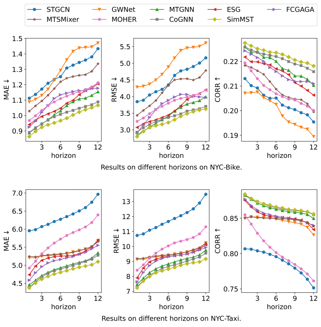
Figure 3: Prediction results on different horizons on NYC dataset.

We show the overall prediction performance of all the methods in Table IV and present the results on different horizons in Figure 3. We observe that our approach achieves the best performance in most cases even if its framework is quite simple, and several conclusions can be further summarized: Firstly, adaptively learning spatial relationships is essential for spatial-temporal data modeling. Compared with STGCN, GWNet, and MTGNN achieve better performance, indicating the predefined relation matrix can not fully capture the spatial relationships between regions, while the learned matrix reflects the inherent relationship more effectively. Secondly, modeling the relationships between multiple modes is beneficial. Although both STGCN and MOHER use predefined graphs, MOHER surpasses STGCN in most cases by considering multiple modes. Similarly, though CoGNN and MTGNN automatically learn the spatial relationships, CoGNN often performs better than MTGNN as it constructs a heterogeneous graph to capture the impacts from different modes. Finally, SimMST consistently outperforms the existing methods in most cases by using a quite simple architecture, which demonstrates its effectiveness in learning the temporal dependencies, cross-mode spatial relationships, and channel correlations in multi-mode spatial-temporal data.

IV-E Importance of Modeling Multi-mode Relationships

In this part, we aim to verify 1) the importance of modeling the relationships of multiple modes; and 2) the generalizability and efficacy of the proposed cross-mode spatial relationships learning (CSRL) component.

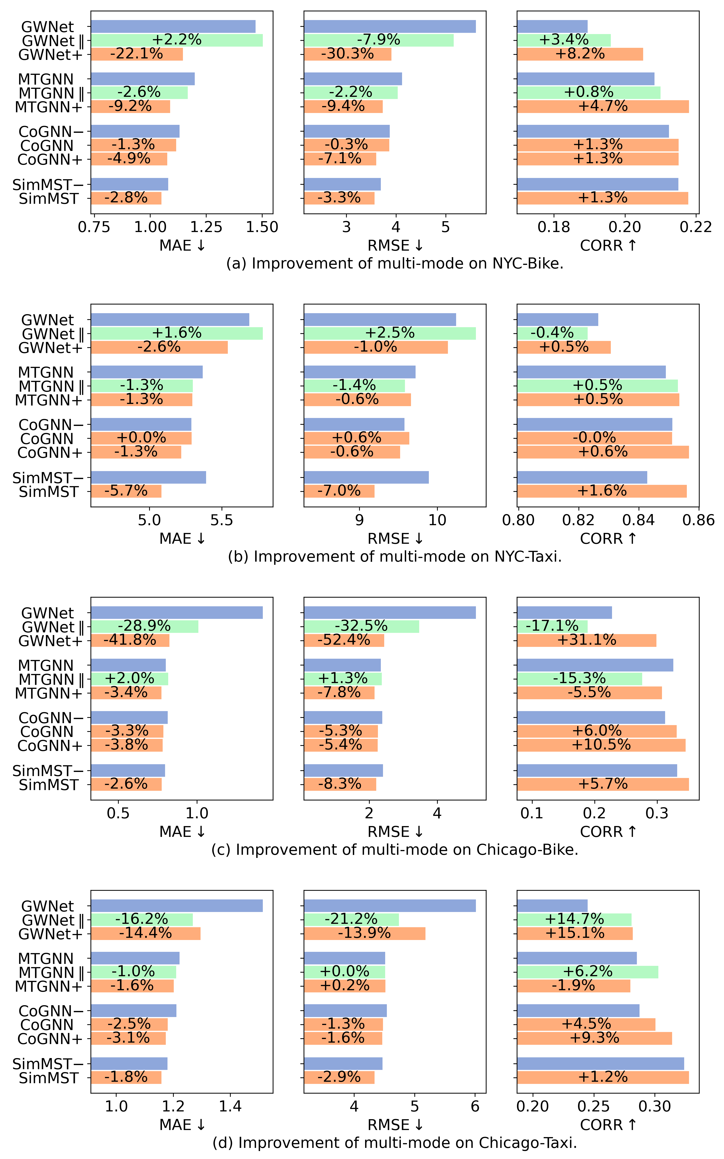
Figure 4: Performance ($H=12$) of different variants on the NYC and Chicago datasets. Blue/Mint/Orange bars denote the performance of methods without modeling multi-mode relationships / with naive combinations of multiple modes / with the capturing of multi-mode relationships. Metric differences compared to blue bars are marked. CoGNN+ refers to substituting its original multi-mode modeling module with our proposed CSRL component.

We first choose GWNet and MTGNN as two representative single-mode methods, which achieve relatively better performance. Then, we provide two ways to adapt them for handling multi-mode spatial-temporal data. One naive way is to treat the observations from multiple modes as different features and combine them together as the inputs for each model. We denote such variants as GWNet $\|$ and MTGNN $\|$. Another way is to integrate our CSRL component into the models and enable them to capture multi-mode relationships. We denote these variants as GWNet+ and MTGNN+. Also, for multi-mode spatial-temporal data modeling methods, we remove the multi-mode modeling module in CoGNN and the proposed SimMST, and denote the variants CoGNN- and SimMST-. Further, we substitute the multi-mode modeling module in CoGNN with the proposed CSRL component and denote it as CoGNN+. We show the performance of all the above methods on the NYC and Chicago datasets in Figure 4.

From Figure 4, we find that 1) combining the observations from multiple modes as input features can help the single-mode methods perform better in most cases, which shows the importance of considering cross-mode information; 2) the proposed cross-mode spatial relationships learning (CSRL) component can effectively improve the model performance further and leads to better performance than the naive combinations of multiple modes, which indicates the necessity of designing customized modules and demonstrates its effectiveness and generalizability; 3) after removing the multi-mode relationship module in CoGNN and our SimMST (CoGNN- v.s. CoGNN and SimMST- v.s. SimMST), the results become worse, which shows the necessity of learning the relationships of multiple modes; 4) by substituting the original multi-mode modeling module of CoGNN with our CSRL component (CoGNN v.s. CoGNN+), CoGNN achieves higher performance, thus demonstrating the efficacy of our proposed CSRL component.

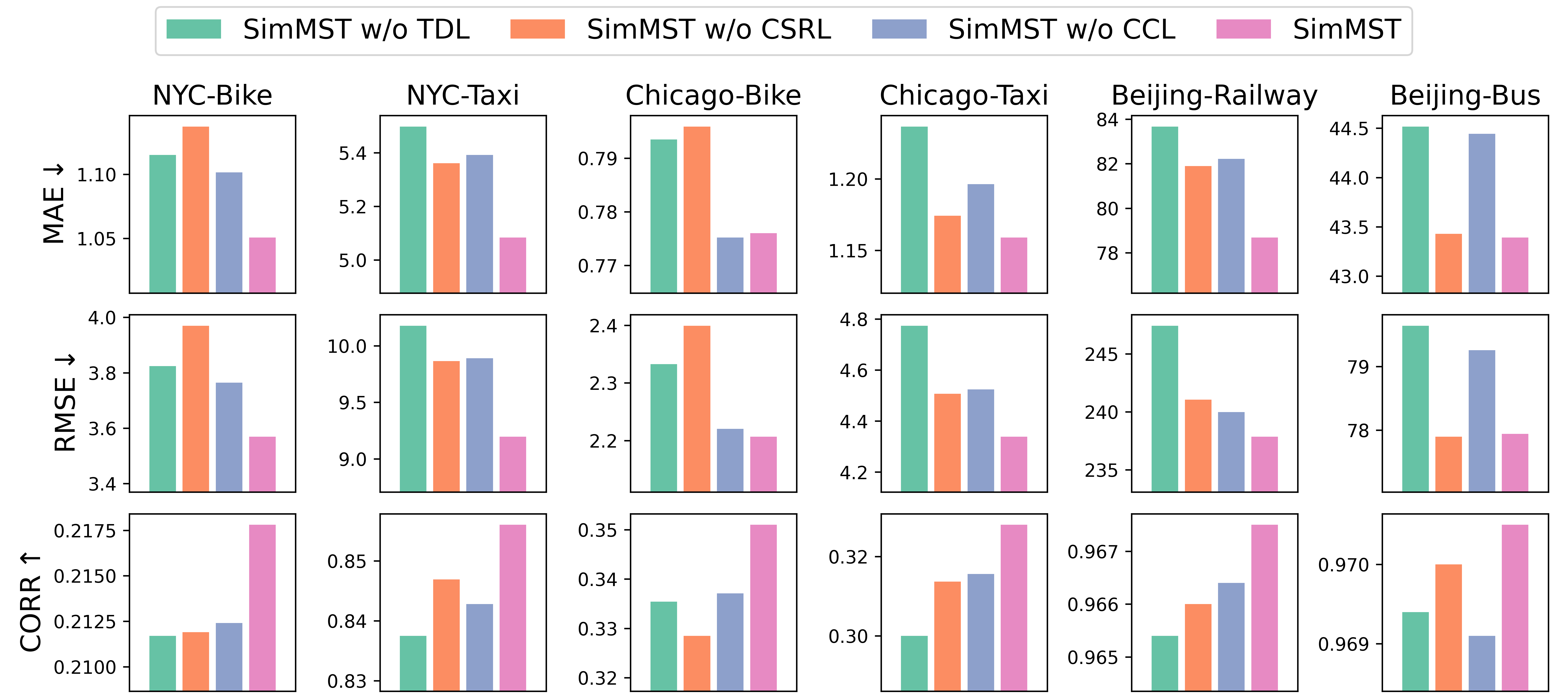
Figure 5: Effects of different components on all three datasets. Performances with $H=12$ are reported.

IV-F Ablation Study

We further conduct an ablation study to validate the effectiveness of the proposed Temporal Dependencies Learning (TDL) component, Cross-mode Spatial Relationships Learning (CSRL) component, and Channel Correlations Learning (CCL) component. We remove TDL, CSRL, and CCL components from the proposed SimMST, and denote the remaining parts as SimMST w/o TDL, SimMST w/o CSRL, and SimMST w/o CCL, respectively. The results of different variants on all three datasets are shown in Figure 5.

From Figure 5, we observe that SimMST achieves the best performance when using all three components. Removing any component will degrade the performance. To be specific, TDL captures the evolutionary pattern of each region in the temporal dimension. CSRL propagates the information between regions under multiple modes to simultaneously exploit the cross-mode and spatial relationships. CCL enhances the model capacity by learning channel correlations. Hence, the contribution of each component is verified.

IV-G Model Efficiency Comparison

Compared with previous methods, another advantage of our approach stems from its simple framework with lower model complexity. Therefore, in this part, we validate the efficiency of our approach by comparing the parameter size and the inference time with baselines. Moreover, we conduct experiments on some variants of SimMST by using seasonality configuration (denoted as SimMST-Season), recurrent-based module (e.g. GRU, denoted as SimMST-RNN) and Attention-based module (e.g. Transformer, denoted as SimMST-Attn) as TDL implementations. The experimental results on all the datasets are shown in Table V.

TABLE V: Comparison of parameter size, inference time, and performance on all datasets.

Dataset	Methods	Bike/Railway MAE-12	Taxi/Bus MAE-12	Relative Performance	Parameter Size	Relative Size	Inference Time (s/epoch)	Relative Time
NYC	MOHER	1.213	6.397	-16.9%	92,492	-58.0%	1.77	+14.4%
	CoGNN	1.117	5.292	-4.9%	932,632	+323.7%	2.26	+46.3%
	GWNet+	1.168	5.545	-9.2%	538,332	+144.5%	6.74	+335.9%
	MTGNN+	1.089	5.297	-3.7%	995,876	+352.4%	2.19	+41.8%
	SimMST-Season	1.071	5.100	-1.1%	226,782	+3.0%	1.51	-2.5%
	SimMST-RNN	1.064	5.122	-0.9%	295,694	+34.3%	1.95	+26.4%
	SimMST-Attn	1.105	5.099	-2.5%	424,718	+92.9%	4.08	+163.7%
	SimMST	1.051	5.089	-	220,140	-	1.55	-
Chicago	MOHER	0.883	1.391	-14.4%	92,492	-57.5%	1.67	+17.3%
	CoGNN	0.800	1.189	-2.7%	874,264	+302.1%	2.07	+45.4%
	GWNet+	0.830	1.314	-9.1%	526,892	+142.4%	6.49	+355.7%
	MTGNN+	0.773	1.202	-1.6%	941,004	+332.8%	2.16	+51.9%
	SimMST-Season	0.779	1.147	+0.3%	224,046	+3.1%	1.40	-1.5%
	SimMST-RNN	0.798	1.170	-1.8%	409,134	+88.2%	1.78	+25.3%
	SimMST-Attn	0.782	1.157	-0.2%	425,262	+95.6%	3.76	+164.1%
	SimMST	0.776	1.159	-	217,404	-	1.42	-
Beijing	MOHER	150.780	66.926	-41.3%	92,492	-53.6%	0.80	+0.4%
	CoGNN	102.099	51.011	-18.8%	493,336	+147.2%	1.08	+35.7%
	GWNet+	103.283	50.351	-18.6%	536,812	+169.0%	5.21	+557.3%
	MTGNN+	108.696	50.291	-20.5%	582,892	+192.1%	1.24	+56.7%
	SimMST-Season	77.939	42.333	+1.9%	206,190	+3.3%	0.80	+0.7%
	SimMST-RNN	77.470	42.196	+2.3%	391,278	+96.1%	0.95	+20.0%
	SimMST-Attn	88.881	46.068	-8.5%	407,406	+104.2%	1.96	+147.4%
	SimMST	77.567	44.121	-	199,548	-	0.79	-

Concretely, on the NYC/Chicago/Beijing dataset, the proposed SimMST achieves 109.6%/ 117.6%/ 162.5% accelerations in time, 65.6%/ 64.3%/ 53.2% reductions in space, and 8.4%/ 5.5%/ 33.3% improvements on average. The significant decreases in inference time and parameter size demonstrate the efficiency and lightweight property of our approach. Though our SimMST additionally learns the multi-mode relation matrices, it brings better performance and the overall simple framework still guarantees that SimMST enjoys a faster speed.

Moreover, compared with complex components such as RNN and Attention, SimMST with MLPs achieves comparable performance despite its simple structure. This suggests that multi-mode spatial-temporal data can be well modeled by a simple framework and complex modules may be unnecessary.

IV-H Visualization

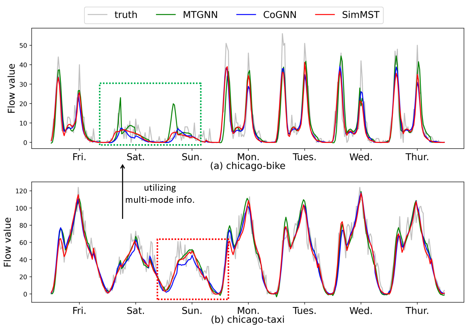
Figure 6: Forecasting visualizations of a case region (id #242) on Chicago dataset. Grey curves refer to the truth observations and green, blue, and red curves respectively refer to the predictions of MTGNN, CoGNN, and SimMST. Only the first 7 days in the test set (6/17/2016 - 6/23/2016) are shown.

We provide a case study to demonstrate the importance of modeling multi-mode relationships and the effectiveness of the proposed method. Figure 6 shows the future traffic demands predicted by MTGNN, CoGNN, and SimMST and the ground truths of a case region on the Chicago dataset.

Despite all methods largely approximate the truth demands, their prediction details are not identical: 1) Compared with methods with multi-mode modeling, single-mode method fails to correctly predict the bike demands on weekends. Specifically, MTGNN mistakenly predicts a peak in the morning on weekends (see green box in the figure), while multi-mode methods (CoGNN and SimMST) can utilize the information from taxi demands and provide more accurate predictions. 2) SimMST is generally more accurate and robust than CoGNN, which can be inferred from the green and red boxes in the figure. With fewer parameters, SimMST can better avoid overfitting the noises of training data and yield smoother predictions.

V Related Work

In this section, we review the related work and show the differences between previous studies and our work, including multi-mode spatial-temporal data modeling methods, and simple frameworks in different fields.

V-A Multi-mode Spatial-Temporal Data Modeling

Due to the importance of spatial-temporal data, a number of efforts have been made on modeling spatial-temporal data. Most of the existing methods mainly focus on learning from a single mode [1, 2, 3, 7, 9, 4, 10, 11, 5, 12, 6, 13]. For example, [1] combined diffusion graph convolution network on predefined graphs and gated recurrent units for modeling traffic data. STGCN [2] applied purely convolutional structures to jointly extract spatial-temporal features for traffic speed forecasting. [7, 5, 23, 24] designed GNN-based frameworks to exploit inherent spatial relationships. ESG [6] constructed multiple evolutionary graph structures to model the dynamic interactions of time series. However, these methods ignore the relationships between the data from multiple modes, which are pervasive in many real-world scenarios.

In recent years, very few researchers investigated the modeling of multi-mode spatial-temporal data. One part of the methods restricted the studied objects on regular grids in the space [18, 19, 16, 20], and thus limited the models’ usability in scenarios with irregular objects. Another part of the methods applied GNNs to propagate information along the connections between regions. STC-GNN [25] learned pairwise similarity between modes and proposed a spatial-temporal encoder-decoder framework. MOHER [21] built graphs with predefined geographical and functional similarities and proposed a propagation mechanism to explore both multi-mode and spatial relationships. CoGNN [17] constructed a heterogeneous graph to learn the inherent spatial relationships of multiple transportation modes with spatial-temporal convolutional networks.

We conclude that previous methods either neglect the multi-mode relationships or need sophisticated modules with higher model complexity. In this paper, we simultaneously capture the temporal dependencies, cross-mode spatial relationships, and channel correlations for modeling multi-mode spatial-temporal data with lower space and time complexity.

V-B Simple Frameworks in Different Fields

Recently, there is an increasing interest in designing simple frameworks in a variety of fields. In computer vision, [26], [27] and [28] abandoned both the convolution and attention operations by presenting MLP-based architectures for image classification. [29] further presented two MLP-based layers for intra-frame and inter-frame modeling respectively for video representation learning. In sequential recommendation, [30] simplified GCN and learned user and item embedding by linear propagation on user-item interaction graphs. [31] replaced the multi-head self-attention layers in Transformer with filter-enhanced MLP layers. MLP4Rec [32] developed a tri-directional fusion scheme to coherently capture sequential, cross-channel, and cross-feature correlations by MLPs. [33] present a succinct architecture that is solely built on the fully connected networks without nonlinear activation functions for temporal sets modeling. For traffic forecasting, FCGAGA [12] employed learnable time gates to model temporal seasonality and hard graph gates to model spatial and temporal relationships at the same time with fully connected layers. MTS-Mixer [13] replaced attention modules with factorized multi-layer perceptrons to capture temporal and channel dependencies. x The above methods have shown the potential of simple architectures. In this paper, we design a simple framework for modeling multi-mode spatial-temporal data to bring both effectiveness and efficiency together.

VI Conclusion

In this paper, we studied the problem of multi-mode spatial-temporal data modeling. Considering the fact that existing methods either failed to capture the multi-mode relationships or were built on complicated modules, we investigated the possibility of designing a simple framework for such a problem. We presented a cross-mode spatial relationships learning component to capture the correlations between multiple modes, which is general and applicable to existing spatial-temporal data modeling methods. We also utilized MLPs to capture the temporal dependencies and channel correlations, which are simple yet effective. Extensive experiments on real-world multi-mode traffic datasets not only showed the effectiveness and efficiency of our approach but also demonstrated the generability of our cross-mode spatial relationships learning module. Our work encourages future research to rethink the key factors for spatial-temporal data modeling and indicates the potential of simple architectures.

Zihang Liu is currently a second-year M.S. student in Computer Science and Engineering from Beihang University. He received the B.S. degree in 2021. His research interests include time-series data mining, recommendation system, and graph neural networks.

Le Yu received the B.S. degree in the School of Computer Science and Engineering at Beihang University, Beijing, China, in 2019. He is currently a fourth-year computer science Ph.D. student in the School of Computer Science and Engineering at Beihang University. His research interests include temporal data mining, machine learning, and graph neural networks.

Tongyu Zhu received the B.S. degree from Tsinghua University in 1992, and the M.S. degree from Beihang University in 1999. He is currently an associate professor with the State Key Laboratory of Software Development Environment in School of Computer Science, Beihang University, Beijing, China. His research interests include intelligent traffic information processing and network application.

Leilei Sun received the B.S., M.S. and Ph.D. degree from Dalian University of Technology in 2009, 2012, and 2017 respectively. He is currently an associate professor with the State Key Laboratory of Software Development Environment (SKLSDE) at School of Computer Science, Beihang University. He was a postdoctoral research fellow from 2017 to 2019 at Tsinghua University. His research interests include machine learning and data mining.

References

- [1] Y. Li, R. Yu et al., “Diffusion Convolutional Recurrent Neural Network: Data-Driven Traffic Forecasting,” in International Conference on Learning Representations, 2018.
- [2] B. Yu, H. Yin, and Z. Zhu, “Spatio-Temporal Graph Convolutional Networks: A Deep Learning Framework for Traffic Forecasting,” in Proceedings of the Twenty-Seventh International Joint Conference on Artificial Intelligence, 2018, pp. 3634–3640.
- [3] X. Yi, J. Zhang et al., “Deep distributed fusion network for air quality prediction,” in Proceedings of the 24th ACM SIGKDD International Conference on Knowledge Discovery & Data Mining. ACM, 2018, pp. 965–973.
- [4] C. Wen, S. Liu et al., “A novel spatiotemporal convolutional long short-term neural network for air pollution prediction,” Science of the total environment, vol. 654, pp. 1091–1099, 2019.
- [5] Z. Wu, S. Pan et al., “Connecting the Dots: Multivariate Time Series Forecasting with Graph Neural Networks,” in Proceedings of the 26th ACM SIGKDD International Conference on Knowledge Discovery & Data Mining, 2020, pp. 753–763.
- [6] J. Ye, Z. Liu et al., “Learning the Evolutionary and Multi-scale Graph Structure for Multivariate Time Series Forecasting,” in Proceedings of the 28th ACM SIGKDD Conference on Knowledge Discovery and Data Mining, 2022, pp. 2296–2306.
- [7] Z. Wu, S. Pan et al., “Graph WaveNet for Deep Spatial-Temporal Graph Modeling,” in Proceedings of the Twenty-Eighth International Joint Conference on Artificial Intelligence, 2019, pp. 1907–1913.
- [8] S. Wang, J. Cao et al., “Deep learning for spatio-temporal data mining: A survey,” IEEE Trans. Knowl. Data Eng., vol. 34, no. 8, pp. 3681–3700, 2022.
- [9] S. Guo, Y. Lin et al., “Attention Based Spatial-Temporal Graph Convolutional Networks for Traffic Flow Forecasting,” in Proceedings of the AAAI Conference on Artificial Intelligence, vol. 33, 2019, pp. 922–929.
- [10] W. Chen, L. Chen et al., “Multi-range attentive bicomponent graph convolutional network for traffic forecasting,” in The Thirty-Fourth AAAI Conference on Artificial Intelligence. AAAI Press, 2020, pp. 3529–3536.
- [11] C. Zheng, X. Fan et al., “GMAN: A graph multi-attention network for traffic prediction,” in The Thirty-Fourth AAAI Conference on Artificial Intelligence. AAAI Press, 2020, pp. 1234–1241.
- [12] B. N. Oreshkin, A. Amini et al., “FC-GAGA: Fully Connected Gated Graph Architecture for Spatio-Temporal Traffic Forecasting,” in Proceedings of the AAAI Conference on Artificial Intelligence, vol. 35, 2021, pp. 9233–9241.
- [13] Z. Li, Z. Rao, L. Pan, and Z. Xu. MTS-Mixers: Multivariate Time Series Forecasting via Factorized Temporal and Channel Mixing. [Online]. Available: http://arxiv.org/abs/2302.04501
- [14] M. Defferrard, X. Bresson et al., “Convolutional neural networks on graphs with fast localized spectral filtering,” in Advances in Neural Information Processing Systems, 2016, pp. 3837–3845.
- [15] B. N. Oreshkin, D. Carpov et al., “N-BEATS: Neural basis expansion analysis for interpretable time series forecasting,” in International Conference on Learning Representations, 2020.
- [16] J. Ye, L. Sun et al., “Co-Prediction of Multiple Transportation Demands Based on Deep Spatio-Temporal Neural Network,” in Proceedings of the 25th ACM SIGKDD International Conference on Knowledge Discovery & Data Mining, 2019, pp. 305–313.
- [17] M. Liu, B. Du, and L. Sun, “Co-Prediction of Multimodal Transportation Demands With Self-learned Spatial Dependence,” in 2021 IEEE International Conference on Big Data (Big Data), 2021, pp. 824–833.
- [18] Y. Liang, S. Ke et al., “GeoMAN: Multi-level attention networks for geo-sensory time series prediction,” in Proceedings of the 27th International Joint Conference on Artificial Intelligence, 2018, pp. 3428–3434.
- [19] C. Huang, C. Zhang et al., “MiST: A Multiview and Multimodal Spatial-Temporal Learning Framework for Citywide Abnormal Event Forecasting,” in The World Wide Web Conference, 2019, pp. 717–728.
- [20] J. Deng, X. Chen et al., “The Pulse of Urban Transport: Exploring the Co-evolving Pattern for Spatio-temporal Forecasting,” ACM Transactions on Knowledge Discovery from Data, vol. 15, no. 6, pp. 103:1–103:25, 2021.
- [21] Q. Zhou, J. Gu et al., “Modeling Heterogeneous Relations across Multiple Modes for Potential Crowd Flow Prediction,” in Proceedings of the AAAI Conference on Artificial Intelligence, vol. 35, 2021, pp. 4723–4731.
- [22] A. Paszke, S. Gross et al., “PyTorch: An Imperative Style, High-Performance Deep Learning Library,” in Advances in Neural Information Processing Systems, vol. 32, 2019.
- [23] L. Bai, L. Yao et al., “Adaptive Graph Convolutional Recurrent Network for Traffic Forecasting,” in Advances in Neural Information Processing Systems, vol. 33, 2020, pp. 17 804–17 815.
- [24] J. Choi, H. Choi et al., “Graph Neural Controlled Differential Equations for Traffic Forecasting,” in Proceedings of the AAAI Conference on Artificial Intelligence, vol. 36, 2022, pp. 6367–6374.
- [25] Z. Wang, R. Jiang et al., “Spatio-Temporal-Categorical Graph Neural Networks for Fine-Grained Multi-Incident Co-Prediction,” in Proceedings of the 30th ACM International Conference on Information & Knowledge Management, 2021, pp. 2060–2069.
- [26] I. O. Tolstikhin, N. Houlsby et al., “MLP-Mixer: An all-MLP Architecture for Vision,” in Advances in Neural Information Processing Systems, vol. 34, 2021, pp. 24 261–24 272.
- [27] H. Touvron, P. Bojanowski et al., “ResMLP: Feedforward networks for image classification with data-efficient training,” 2021.
- [28] T. Yu, X. Li et al., “S2-MLP: Spatial-Shift MLP Architecture for Vision,” in Proceedings of the IEEE/CVF Winter Conference on Applications of Computer Vision, 2022, pp. 297–306.
- [29] D. J. Zhang, K. Li, Y. Wang, Y. Chen, S. Chandra, Y. Qiao, L. Liu, and M. Z. Shou, “MorphMLP: An Efficient MLP-Like Backbone for Spatial-Temporal Representation Learning,” in Computer Vision – ECCV 2022, S. Avidan, G. Brostow, M. Cissé, G. M. Farinella, and T. Hassner, Eds., pp. 230–248.
- [30] X. He, K. Deng et al., “LightGCN: Simplifying and Powering Graph Convolution Network for Recommendation,” in Proceedings of the 43rd International ACM SIGIR Conference on Research and Development in Information Retrieval, 2020, pp. 639–648.
- [31] K. Zhou, H. Yu et al., “Filter-enhanced MLP is all you need for sequential recommendation,” in Proceedings of the ACM Web Conference 2022, 2022, pp. 2388–2399.
- [32] M. Li, X. Zhao et al., “MLP4Rec: A Pure MLP Architecture for Sequential Recommendations,” in International Joint Conferences on Artificial Intelligence Organization, 2022.
- [33] L. Yu, Z. Liu, T. Zhu, L. Sun, B. Du, and W. Lv, “Predicting Temporal Sets with Simplified Fully Connected Networks,” in Proceedings of the AAAI Conference on Artificial Intelligence, vol. 37, no. 4, pp. 4835–4844.