Quantitative stability
for overdetermined nonlocal problems
with parallel surfaces
and investigation of the stability exponents

Abstract.

In this article, we analyze the stability of the parallel surface problem for semilinear equations driven by the fractional Laplacian. We prove a quantitative stability result that goes beyond that previously obtained in [Cir+23].

Moreover, we discuss in detail several techniques and challenges in obtaining the optimal exponent in this stability result. In particular, this includes an upper bound on the exponent via an explicit computation involving a family of ellipsoids. We also sharply investigate a technique that was proposed in [Cir+18] to obtain the optimal stability exponent in the quantitative estimate for the nonlocal Alexandrov’s soap bubble theorem, obtaining accurate estimates to be compared with a new, explicit example.

1. Introduction and main results

1.1. The long-standing tradition of overdetermined problems

Overdetermined problems are a broad class of partial differential equations (PDEs) where ‘too many conditions’ are imposed on the solution. Since not every region will admit a solution which satisfies all the conditions, the objective in the study of overdetermined problems is to classify those regions which do admit solutions.

Often, overdetermined problems arise naturally in applications as a combination of a well-posed partial differential equation (PDE) which describes the dynamics of a given physical system, as well as an extra condition, often referred to as the overdetermined condition, which describes a property or an optimal quality you would like the solution to possess. As such, overdetermined problems have a close relationship with optimization, free boundary problems and calculus of variations, particularly shape optimization, as well as many other applications including fluid mechanics, solid mechanics, thermodynamics, electrostatics, see [Ser71, FG08, HP18, DPV21].

The study of overdetermined problems began in the early 1970’s with the celebrated paper of Serrin [Ser71]. In this influential paper, Serrin proved that, given a bounded domain $\Omega\subset\mathbb{R}^{n}$ with $C^{2}$ boundary and $f\in C^{0,1}_{\text{loc}}(\mathbb{R})$, if there exists a positive solution $u\in C^{2}(\overline{\Omega})$ that satisfies the Dirichlet boundary value problem

(1.3) $$\left\{\begin{array}[]{r@{ \ }l @{\quad\: \;} l}-\Delta u&=f(u)\hfil\quad\>&\text{in }\Omega,\\ u&=0\hfil\quad\>&\text{on }\partial\Omega,\end{array}\right.$$

as well as the overdetermined condition

(1.4) $$\partial_{\nu}u =c\qquad\text{on }\partial\Omega$$

for some constant $c\in\mathbb{R}\setminus\{0\}$, then $\Omega$ must be a ball. Here $\nu$ is the unit outward pointing normal to $\partial\Omega$ and $\partial_{\nu}u=\nabla u\cdot\nu$. The proof relies on a powerful technique, now known as the method of moving planes, a refinement of a reflection principle conceived by Alexandrov in [Ale62] to prove the so-called soap bubble theorem, which states that the only connected closed hypersurfaces embedded in a space form with everywhere constant mean curvature are spheres.

Since the work of Alexandrov and Serrin, the analysis of overdetermined problems and the method of moving planes has seen intense research activity. Some of the literature on the method of moving planes, overdetermined problems, and symmetry in PDE include:

• Alternate/incomplete overdetermined conditions: One can consider elliptic equations such (1.3) or otherwise with an alternate overdetermined condition to (1.4), see [HP98, FG08, BHS14, DPV21]. The parallel surface problem fits into this category, see below for references.

• Integral identities: Integral identities such as the Pohozaev identity are often employed in the analysis of overdetermined problems, providing an alternative approach to the method of moving planes. Such an alternative approach was pioneered in [Wei71] and then further developed in, e.g., [PS89, GL89, Bra+08, CS09, QX17, CV19, MP20, MP20a].

• Nonlinear elliptic equations: The original paper of Serrin [Ser71] dealt with uniformly elliptic quasilinear equations including equations of mean curvature type. Other (possibly degenerate) quasilinear and fully nonlinear equations have been analyzed [GL89, DS07, FK08, Bra+08, BK11, BD13, SS15].

• Symmetry: The method of moving planes was famously used to prove symmetry results for solutions to semilinear PDE in domains with symmetry in [GNN79, GNN81]. For this type of results, an alternative approach which combines Pohozaev identity and isoperimetric-type inequalities was pioneered in [Lio81] and then further developed in [KP94, Ser13, DPV22].

• Nonlocal operators: For overdetermined problems and symmetry for nonlocal equations, see [FJ15, Cab+18, Cir+18, SV19, Dip+22, Cir+23].

1.2. The nonlocal parallel surface problem and the main results of this paper

In this paper, we are concerned with the nonlocal parallel surface problem. The context of this problem is as follows: Let $n$ be a positive integer and $s\in(0,1)$. Suppose that $G$ is an open bounded subset of $\mathbb{R}^{n}$ and let $\Omega=G+B_{R}$ for some $R>0$, where $A+B$ is the Minkowski sum of sets defined by

$$A+B=\{a+b\text{ s.t. }a\in A,b\in B\}.$$

Moreover, let $(-\Delta)^{s}$ denote the fractional Laplacian defined by

$$(-\Delta)^{s}u(x) =c_{n,s}\mathrm{P.V.}\int_{\mathbb{R}^{n}}\frac{u(x)-u(y)}{|x-y|^{n+2s}}\mathop{}\!dy$$

where $c_{n,s}$ is a positive normalization constant and $\mathrm{P.V.}$ denotes the Cauchy principle value. Also, assume that $f:\mathbb{R}\to\mathbb{R}$ is locally Lipschitz and satisfies $f(0)\geqslant 0$. Then, the nonlocal parallel surface problem asks: if there exists a function $u$ that satisfies (in an appropriate sense) the equation

(1.8) $$\left\{\begin{array}[]{r@{ \ }l @{\quad\: \;} l}(-\Delta)^{s}u&=f(u)\hfil\quad\>&\text{in }\Omega,\\ u&=0\hfil\quad\>&\text{in }\mathbb{R}^{n}\setminus\Omega,\\ u&\geqslant 0\hfil\quad\>&\text{in }\mathbb{R}^{n},\end{array}\right.$$

as well as the overdetermined condition

(1.9) $$u=\text{constant}\qquad\text{on }\partial G,$$

then is $\Omega$ necessarily a ball?

This question is referred to as the rigidity problem for the parallel surface problem. Furthermore, one can ask about the stability of this problem, that is, heuristically, if $u$ satisfies (1.8) and ‘almost’ satisfies (1.9) then is $\Omega$ ‘almost’ a ball? This is the subject of the current article. Of course, one must be precise by what one means by ‘almost’—this will be made clear in the proceeding paragraphs as we describe the literature and our main results.

The local analogue of the parallel surface problem (i.e. the case $s=1$) was introduced in [Sha12] as a discrete analogue of the original Serrin’s problem. Moreover, it also appears in [MS10, CMS15] in the context of invariant isothermic surfaces of a nonlinear non-degenerate fast diffusion equation.

To see why the parallel surface problem can be viewed as a discrete analogue of Serrin’s problem, consider that $u\in C^{2}(\overline{\Omega})$ satisfies (1.3) as well as $u=c_{k}>0$ on an countably infinite family of parallel surfaces $\Gamma_{k}$ that are a distance $1/k$ from the boundary of $\Omega$. Then $kc_{k}$ necessarily converges to some $c$ by regularity assumptions on $u$ and $u$ satisfies (1.4). Consequently, $\Omega$ must be a ball.

To reiterate, in the parallel surface problem there is only a single parallel surface (not a family as just described); regardless, this was enough to prove in [Sha12, CMS15] the rigidity result: if there exists a solution to (1.3) satisfying (1.9) then $\Omega$ must be a ball.

Subsequently, in [CMS16], the stability of (1.8) for the local problem was addressed. In that article, the authors used the shape functional

$$\rho(\Omega)=\inf\big{\{}R-r\text{ s.t. }B_{r}(x)\subset\Omega\subset B_{R}(x)\text{ for some }x\in\Omega\big{\}}$$

to quantify how close $\Omega$ is to being a ball and the semi-norm

$$[u]_{\partial G}=\sup_{\begin{subarray}{c}x,y\in\partial G\\ x\neq y\end{subarray}}\bigg{\{}\frac{|u(x)-u(y)|}{|x-y|}\bigg{\}}$$

to quantify how close $u$ is to being constant on $\partial\Omega$. They showed, under reasonable assumptions on $\Omega$, that

(1.10) $$\rho(\Omega)\leqslant C[u]_{\partial G}.$$

Moreover, for the nonlocal parallel surface problem, the rigidity problem was answered affirmatively in [Cir+23] for the case $f=1$ and [Dip+22] for general $f$. Moreover, [Cir+23] also addressed the stability problem (still for the case $f=1$) and showed that

(1.11) $$\rho(\Omega)\leqslant C[u]_{\partial G}^{\frac{1}{s+2}}.$$

It is interesting to observe that (1.11) is sub-optimal in the sense that it does not recover the estimate (1.10) when $s=1$. This is due to the nonlocality of the fractional Laplacian which caused contributions from mass ‘far away’ to have a significant effect on the analysis.

This leads us to our main result.

Theorem 1.1.

oAZAv7vy Let $G$ be an open bounded subset of $\mathbb{R}^{n}$ and $\Omega=G+B_{R}$ for some $R>0$. Furthermore, let $\Omega$ and $G$ have $C^{1}$ boundary, and let $f\in C^{0,1}_{\mathrm{loc}}(\mathbb{R})$ be such that $f(0)\geqslant 0$. Suppose that $u$ satisfies (1.8) in the weak sense.

Then,

(1.12) $$\rho(\Omega) \leqslant C[u]_{\partial G}^{\frac{1}{s+2}}$$

with

$$C:=C(n,s)\left[\frac{(\max\{1,\operatorname{diam}\Omega\})^{n+2s}\big{(}1+(\operatorname{diam}\Omega)^{2s}[f]_{C^{0,1}([0,\|u\|_{L^{\infty}(\Omega)}])}\big{)}}{R^{s}\big{(}f(0)+\|u\|_{L_{s}(\mathbb{R}^{n})}\big{)}}+(\operatorname{diam}\Omega)^{n-1}+\frac{|\Omega|}{R}\right]\\ \times\frac{(\operatorname{diam}\Omega)^{n+2s+3}}{R^{2s}|\Omega|}\left(1+R^{2s}[f]_{C^{0,1}([0,\|u\|_{L^{\infty}(\Omega)}])}\right).$$

For the precise definition of a solution satisfying (1.8) in the weak sense, see Section 2.

oAZAv7vy is a direct extension of [Cir+23] to the case $f\neq 1$. Moreover, oAZAv7vy relaxes some of the regularity assumptions on $\Omega$ appearing in [Cir+23]. It is clear that the dependence on the volume $|\Omega|$ in the constant of Theorem LABEL:oAZAv7vy can be removed by means of the following bounds

$$|B_{1}|R^{n}\leqslant|\Omega|\leqslant|B_{1}|(\operatorname{diam}\Omega)^{n},\text{ where }|B_{1}|\text{ is the volume of the unit ball in }\mathbb{R}^{n},$$

which hold true in light of the monotonicity of the volume with respect to inclusion.

Currently, an important open problem for the nonlocal parallel surface problem is to understand the optimality of oAZAv7vy. Indeed, let $\overline{\beta}(s)$ be the optimal exponent in (1.12) defined as the supremum over $\beta\in\mathbb{R}$ such that if $u=u_{f}$ is a weak solution of (1.8) for some $f$ satisfying the assumptions of oAZAv7vy then $\rho(\Omega)\leqslant C[u]_{\partial G}^{\beta}$. In this framework, an explicit expression for $\overline{\beta}$ as a function of $s$ is still unknown. oAZAv7vy implies that $\overline{\beta}(s)\geqslant\frac{1}{s+2}$ and [Sha12, CMS15] establish that $\overline{\beta}(1)=1$, therefore we believe it is an interesting problem to detect optimal stability exponents in the nonlocal setting, also to recover, whenever possible, the classical exponent of the local cases in the limit.

In Section 7, we explicitly construct a family of domains $G_{\varepsilon}$ that are small perturbations of a ball and corresponding solutions $u_{\varepsilon}$ to (1.8) when $f=1$ which satisfy $[u_{\varepsilon}]_{\partial G_{\varepsilon}}\simeq C\rho(\Omega_{\varepsilon})$ as $\varepsilon\to 0^{+}$. This entails the following result:

Theorem 1.2.

O4zCF33o Let $G$ be an open bounded subset of $\mathbb{R}^{n}$ and $\Omega=G+B_{R}$ for some $R>0$. Furthermore, let $\Omega$ and $G$ have $C^{1}$ boundary.

Then, we have that $\overline{\beta}(s)\leqslant 1$.

As far as the authors are aware, these are the only known estimates for $\overline{\beta}(s)$. Furthermore, by considering the case in which $\Omega=\Omega_{\varepsilon}$ is a small perturbation of a ball and exploting interior regularity for the fractional Laplacian, one would expect that $\rho(\Omega_{\varepsilon})\simeq[u_{\varepsilon}]_{\partial G_{\varepsilon}}\simeq\varepsilon$ (up to constant) as $\varepsilon\to 0^{+}$ which suggests that $\overline{\beta}(s)=1$ for all $s\in(0,1]$. In Section 5, we give a broad discussion on some of the challenges that the nonlocality of the fractional Laplacian presents in obtaining this result. In particular, by way of an example via the Poisson representation formula, we show that estimates for a singular integral involving the reciprocal of the distance to the boundary function play a key role in obtaining the anticipated optimal result. This suggests, surprisingly, that fine geometric estimates for the distance function close to the boundary are required to obtain the optimal exponent.

1.3. Scrutiny of the stability exponent

In the recent literature, some inventive methods have been introduced to improve the stability results obtained via the moving plane method. A remarkable one was put forth in [Cir+18]. Roughly speaking, the setting considered in [Cir+18, Proposition 3.1(b)] focused on the critical hyperplane $\pi_{\lambda}=\{x_{n}=\lambda\}$ for the moving plane technique for a set $\Omega$ which contains the ball $B_{r}$ and is contained in the ball $B_{R}$, looked at the symmetric difference between $\Omega$ and its reflection $\Omega^{\prime}$ and obtained a bound on the measure of the set

(1.13) $$\big{\{}x\in\Omega\triangle\Omega^{\prime}\text{ s.t. }\operatorname{dist}(x,\pi_{\lambda})\leqslant\gamma\big{\}}$$

which was linear in both $\gamma$ and $R-r$.

This constituted a fundamental ingredient in [Cir+18] to achieve an optimal stability exponent.

Unfortunately, we believe that, in the very broad generality in which the result is stated in [Cir+18], this statement may not be true, and we present an explicit counter-example.

Nevertheless, in our opinion, a weaker version of [Cir+18, Proposition 3.1(b)] does hold true. We state and prove this new result and check its optimality against the counter-example mentioned above. This construction plays a decisive role in improving the stability exponent.

Though we refer the reader to Section 6 for full details of this strategy, let us anticipate here some important details.

More specifically, in the forthcoming Theorem LABEL:m9q9X2hE, under the additional assumption that the set $\Omega$ is of class $C^{\alpha}$, with $\alpha>1$, we will bound the measure of the set in (1.13), up to constants, by

(1.14) $$\gamma(R-r)^{1-\frac{1}{\alpha}}.$$

We stress that this bound formally recovers exactly the one stated in [Cir+18, Proposition 3.1(b)] when $\alpha=+\infty$.

However, we believe that the bound in (1.14) is optimal and cannot be improved (in particular, while the dependence in $\gamma$ of the estimate above is linear, the dependence in $R-r$, surprisingly, is not!). This will be shown by an explicit counter-example put forth in Theorem 6.6—while the analytical details of this counter-example are very delicate, the foundational idea behind it is sketched in Figure 2 (roughly speaking, the example is obtained by a very small and localized modification of a ball to induce a critical situation at the maximal location allowed by the regularity of the set; the construction is technically demanding since the constraint for the set of “being between two balls” induces two different scales, in the horizontal and in the vertical directions, which in principle could provide different contributions).

As a consequence of the bound (1.14) for the measure of the set in (1.13), as given in m9q9X2hE, the stability exponent $1/(s+2)$ of oAZAv7vy can be improved to $\alpha/(1+\alpha(s+1))$ provided that $\Omega$ is of class $C^{\alpha}$ for $\alpha>1$: we refer to Section 6.2 and thm:improvement for details.

1.4. Organization of paper

The paper is organized as follows. In Section 2, we summarize the notation and basic definitions used throughout the article. In Section 3, we give several quantitative maximum principles—in both the non-antisymmetric and antisymmetric situations—that are required in the proof of oAZAv7vy and, in Section 4, we give the proof of oAZAv7vy.

The remaining sections are broadly focused on the techniques and challenges in obtaining the optimal stability exponent. In Section 5, we discuss the surprising role that fine geometric estimates for the distance function close to the boundary play in the attainment of the optimal exponent. In Section 6, we accurately discuss the possibility of obtaining the optimal exponent and comment about some criticalities in the existing literature, and, in Section 7, we construct an explicit family of solutions which implies O4zCF33o.

2. Preliminaries and notation

In this section we fix the notation that we will use throughout the article and give some relevant definitions. Let $n\geqslant 1$ and $s\in(0,1)$. The fractional Sobolev space $H^{s}(\mathbb{R}^{n})$ is defined as

$$H^{s}(\mathbb{R}^{n})=\big{\{}u\in L^{2}(\mathbb{R}^{n})\text{ such that }[u]_{H^{s}(\mathbb{R}^{n})}<+\infty\big{\}}$$

where $[\cdot]_{H^{s}(\mathbb{R}^{n})}$ is the Gagliardo semi-norm given by

$$[u]_{H^{s}(\mathbb{R}^{n})}=c_{n,s}\int_{\mathbb{R}^{n}}\int_{\mathbb{R}^{n}}\frac{|u(x)-u(y)|^{2}}{|x-y|^{n+2s}}\mathop{}\!dy\mathop{}\!dx$$

where $c_{n,s}$ is the same constant appearing in the definition of the fractional Laplacian. Functions in $H^{s}(\mathbb{R}^{n})$ that are equal almost everywhere are identified. Moreover, the bilinear form associated with $[\cdot]_{H^{s}(\mathbb{R}^{n})}$ is denoted by $\mathcal{E}:H^{s}(\mathbb{R}^{n})\times H^{s}(\mathbb{R}^{n})\to\mathbb{R}$ and is given by

$$\mathcal{E}(u,v)=\frac{c_{n,s}}{2}\int_{\mathbb{R}^{n}}\int_{\mathbb{R}^{n}}\frac{(u(x)-u(y))(v(x)-y(y)}{|x-y|^{n+2s}}\mathop{}\!dy\mathop{}\!dx.$$

We also define the following weighted $L^{1}$ norm via

$$\|u\|_{L_{s}(\mathbb{R}^{n})}=\int_{\mathbb{R}^{n}}\frac{|u(x)|}{1+|x|^{n+2s}}\mathop{}\!dx$$

and the space $L_{s}(\mathbb{R}^{n})$ as

$$L_{s}(\mathbb{R}^{n})=\big{\{}L^{1}_{\mathrm{loc}}(\mathbb{R}^{n})\text{ such that }\|u\|_{L_{s}(\mathbb{R}^{n})}<+\infty\big{\}}.$$

Now, suppose that $\Omega$ is an open, bounded subset of $\mathbb{R}^{n}$ and define the space $\mathcal{H}^{s}_{0}(\Omega)$ by

$$\mathcal{H}^{s}_{0}(\Omega) =\big{\{}u\in H^{s}(\mathbb{R}^{n})\text{ such that }u=0\text{ in }\mathbb{R}^{n}\setminus\Omega\big{\}}.$$

Let $c:\Omega\to\mathbb{R}$ be a measurable function such that $c\in L^{\infty}(\Omega)$ and $g\in L^{2}(\Omega)$. We say that a function $u\in H^{s}(\mathbb{R}^{n})\cap L_{s}(\mathbb{R}^{n})$ satisfies $(-\Delta)^{s}u+cu\geqslant g$ (respectively, $\leqslant$) in the weak sense if

$$\mathcal{E}(u,v)+\int_{\Omega}cuv\mathop{}\!dx\geqslant\int_{\Omega}gv\mathop{}\!dx\qquad(\text{respectively, }\leqslant)$$

for all $v\in\mathcal{H}^{s}_{0}(\Omega)$ with $v\geqslant 0$. In this case, we also say that $u$ is a supersolution (respectively, subsolution) of $(-\Delta)^{s}u+cu=g$ in the weak sense. Moreover, we say a function $u\in H^{s}(\mathbb{R}^{n})\cap L_{s}(\mathbb{R}^{n})$ satisfies $(-\Delta)^{s}u+cu=g$ in the weak sense if

$$\mathcal{E}(u,v)+\int_{\Omega}cuv\mathop{}\!dx=\int_{\Omega}gv\mathop{}\!dx$$

for all $v\in\mathcal{H}^{s}_{0}(\Omega)$. This is equivalent to $u$ being both a weak supersolution and a weak subsolution. Note that we are assuming a priori that weak solutions are in $L_{s}(\mathbb{R}^{n})$.

Next, we describe some notation regarding antisymmetric functions. This is closely related to the notation of the method of moving planes; however, we will defer our explanation of the method of moving planes until Section 4 in the interests of simplicity.

A function $v:\mathbb{R}^{n}\to\mathbb{R}$ is said to be antisymmetric with respect to a plane $T$ if

$$v(Q_{T}(x))=-v(x)\qquad\text{for all }x\in\mathbb{R}^{n}$$

where $Q_{T}:\mathbb{R}^{n}\to\mathbb{R}^{n}$ is the function that reflects $x$ across $T$. Often it will suffice to consider the case $T=\{x_{1}=0\}$, in which case $Q_{T}(x)=x-2x_{1}e_{1}$.

For simplicity, we will refer to $v$ as antisymmetric if it is antisymmetric with respect to the plane $\{x_{1}=0\}$. Moreover, we sometimes write $x^{\prime}$ to denote $Q_{T}(x)$ when it is clear from context what $T$ is.

Finally, some other notation we will employ through the article is: given a set $A\subset\mathbb{R}^{n}$, the function $\chi_{A}:\mathbb{R}^{n}\to\mathbb{R}$ denotes the characteristic function of $A$, given by

$$\chi_{A}(x) =\begin{cases}1,&\text{if }x\in A,\\ 0,&\text{if }x\not\in A,\end{cases}$$

and $\delta_{A}:\mathbb{R}^{n}\to[0,+\infty]$ denotes the distance function to $A$, given by

$$\delta_{A}(x)=\inf_{y\in A}|x-y|.$$

We will denote by $\mathbb{R}^{n}_{+}:=\{x=(x_{1},\dots,x_{n})\in\mathbb{R}^{n}\;{\mbox{s.t.}}\;x_{1}>0\}$ and, given $A\subseteq\mathbb{R}^{n}$, we will denote by $A^{+}:=A\cap\mathbb{R}^{n}_{+}$.

Moreover, if $A$ is open and bounded with sufficiently regular boundary (we only use the case in which $A$ has smooth boundary), we will denote by $\psi_{A}$ the (unique) function in $C^{\infty}(A)\cap C^{s}(\mathbb{R}^{n})$ such that $\psi_{A}$ satisfies

(2.3) $$\left\{\begin{array}[]{r@{ \ }l @{\quad\: \;} l}(-\Delta)^{s}\psi_{A}&=1\hfil\quad\>&\text{in }A,\\ \psi_{A}&=0\hfil\quad\>&\text{in }\mathbb{R}^{n}\setminus A.\end{array}\right.$$

Also, we will use $\lambda_{1}(A)$ to denote the first Dirichlet eigenvalue of the fractional Laplacian.

3. Quantitative maximum principles up to the boundary

The basic idea of the proof of oAZAv7vy is to apply the method of moving planes, as in the proof of the analogous rigidity result [Dip+22, Theorem 1.4], but replace ‘qualitative’ maximum principles, such as the strong maximum principles, with ‘quantitative’ maximum principles, such as the Harnack inequality.

The purpose of this section is to prove several such quantitative maximum principles both in the non-antisymmetric and the antisymmetric setting. In particular, we require that these maximum principles hold up to the boundary of regions with very little boundary regularity. Moreover, we are careful to keep track of precisely how constants depend on relevant quantities since we believe that this may be useful in future analyses of the nonlocal parallel surface problem.

The section is split into two parts: maximum principles for equations without any antisymmetry assumptions and maximum principles for equations with antisymmetry assumptions.

3.1. Equations without antisymmetry

In this subsection, we will give several maximum principles for linear equations with zero-th order terms without any antisymmetry assumptions. This will culminate in a quantitative analogue of the Hopf lemma for non-negative supersolutions of general semilinear equations (see zAPw0npM below).

Our first result is as follows:

Proposition 3.1.

YCl8lL0I Let $\Omega$ be an bounded open subset of $\mathbb{R}^{n}$, $c\in L^{\infty}(\Omega)$, and $g\in L^{2}(\Omega)$ with $g\geqslant 0$. Suppose that $u$ satisfies

$$\left\{\begin{array}[]{r@{ \ }l @{\quad\: \;} l}(-\Delta)^{s}u+cu&\geqslant g\hfil\quad\>&\text{in }\Omega,\\ u&\geqslant 0\hfil\quad\>&\text{in }\mathbb{R}^{n}\end{array}\right.$$

in the weak sense.

Then,

$$u(x) \geqslant C\Big{(}\operatorname*{ess\,inf}_{\Omega}g+\|u\|_{L_{s}(\mathbb{R}^{n})}\Big{)}\delta_{\partial\Omega}^{2s}(x)\qquad\text{for a.e. }x\in\Omega$$

with $C:=C(n,s)(\max\{1,\operatorname{diam}\Omega\})^{-n-2s}\big{(}1+(\operatorname{diam}\Omega)^{2s}\|c^{+}\|_{L^{\infty}(\Omega)}\big{)}^{-1}$.

The proof of YCl8lL0I essentially follows by, at each point $x\in\Omega$, ‘touching’ the solution $u$ from below by $\psi_{B}$ (recall the notation in (2.3)) where $B$ is the largest ball contained in $\Omega$ and centred at $x$. This is similar to the proof of [RS19, Theorem 2.2] where a nonlinear interior analogue of YCl8lL0I was proven. To prove YCl8lL0I, however, some care must be taken since the touching point may occur on the boundary of $\Omega$ (unlike in the interior result of [RS19, Theorem 2.2]) where the PDE does not necessarily hold. Moreover, YCl8lL0I is stated in the context of weak solutions where pointwise techniques no longer make sense, so a simple mollification argument needs to be made. We require the following lemma.

Lemma 3.2.

Voueel7o Let $\rho>0$, $c\in L^{\infty}(B_{\rho})$, and $g\in C^{\infty}_{0}(\mathbb{R}^{n})$ be such that $g\geqslant 0$ in $B_{\rho}$. Suppose that $u\in C^{\infty}_{0}(\mathbb{R}^{n})$ satisfies

$$\left\{\begin{array}[]{r@{ \ }l @{\quad\: \;} l}(-\Delta)^{s}u+cu&\geqslant g\hfil\quad\>&\text{in }B_{\rho},\\ u&\geqslant 0\hfil\quad\>&\text{in }\mathbb{R}^{n}.\end{array}\right.$$

Then,

$$u(x)\geqslant C\Big{(}\inf_{B_{\rho}}g+\|u\|_{L_{s}(\mathbb{R}^{n})}\Big{)}\psi_{B_{\rho}}(x)\qquad\text{for all }x\in B_{\rho}$$

with $C:=C(n,s)(\max\{1,\rho\})^{-n-2s}\big{(}1+\rho^{2s}\|c^{+}\|_{L^{\infty}(B_{\rho})}\big{)}^{-1}$.

We observe that Lemma LABEL:Voueel7o can be seen as a quantitative version of a strong maximum principle (which can be proved directly): in particular, it entails that if $u(x_{0})=0$ for some $x_{0}\in\Omega$, then $u$ vanishes identically.

Proof of Lemma LABEL:Voueel7o.

We will begin by proving the case $\rho=1$. Fix $\varepsilon>0$ small and let $\tau\geqslant 0$ be the largest value such that $u\geqslant\tau\psi_{B_{1-\varepsilon}}$ in $\mathbb{R}^{n}$. Now, by the definition of $\tau$, there exists $x_{0}\in B_{1-\varepsilon}$ such that $u(x_{0})=\tau\psi_{B_{1-\varepsilon}}(x_{0})$. On one hand,

$$(-\Delta)^{s}(u-\tau\psi_{B_{1-\varepsilon}})(x_{0})+c(x_{0})(u-\tau\psi_{B_{1-\varepsilon}})(x_{0}) \geqslant\inf_{B_{1}}g-\tau\big{(}1+c(x_{0})\psi_{B_{1-\varepsilon}}(x_{0})\big{)}$$

$$\geqslant\inf_{B_{1}}g-C(n,s)\big{(}1+\|c^{+}\|_{L^{\infty}(B_{1})}\big{)}\tau.$$

On the other hand, since $|x_{0}-y|^{-n-2s}\geqslant C(n,s)(1+|y|^{n+2s})^{-1}$, we have that

$$(-\Delta)^{s}(u-\tau\psi_{B_{1-\varepsilon}})(x_{0})+c(x_{0})(u-\tau\psi_{B_{1-\varepsilon}})(x_{0}) =-\int_{\mathbb{R}^{n}}\frac{(u-\tau\psi_{B_{1-\varepsilon}})(y)}{|x_{0}-y|^{n+2s}}\mathop{}\!dy$$

$$\leqslant-C(n,s)\int_{\mathbb{R}^{n}}\frac{(u-\tau\psi_{B_{1-\varepsilon}})(y)}{1+|y|^{n+2s}}\mathop{}\!dy$$

$$\leqslant-C(n,s)\big{(}\|u\|_{L_{s}(\mathbb{R}^{n})}-\tau\big{)}.$$

Rearranging gives $\tau\geqslant C(n,s)\big{(}1+\|c^{+}\|_{L^{\infty}(B_{1})}\big{)}^{-1}\big{(}\inf_{B_{1}}g+\|u\|_{L_{s}(\mathbb{R}^{n})}\big{)}$, which implies that

$$u(x) \geqslant C(n,s)\big{(}1+\|c^{+}\|_{L^{\infty}(B_{1})}\big{)}^{-1}\Big{(}\inf_{B_{1}}g+\|u\|_{L_{s}(\mathbb{R}^{n})}\Big{)}\psi_{B_{1-\varepsilon}}.$$

Sending $\varepsilon\to 0^{+}$ gives the result when $\rho=1$.

Now, for the case that $\rho$ is not necessarily 1, let $u_{\rho}(x):=u(\rho x)$. Then

$$(-\Delta)^{s}u_{\rho}+\rho^{2s}c_{\rho} \geqslant\rho^{2s}g_{\rho}\qquad\text{in }B_{1}$$

where $c_{\rho}(x):=c(\rho x)$ and $g_{\rho}(x):=g(\rho x)$, so, for all $x\in B_{\rho}$, we have that

$$u(x) =u_{\rho}(x/\rho)$$

$$\geqslant C(n,s)\big{(}1+\rho^{2s}\|c^{+}_{\rho}\|_{L^{\infty}(B_{1})}\big{)}^{-1}\Big{(}\rho^{2s}\inf_{B_{1}}g_{\rho}+\|u_{\rho}\|_{L_{s}(\mathbb{R}^{n})}\Big{)}\psi_{B_{1}}(x/\rho)$$

$$=C(n,s)\rho^{-2s}\big{(}1+\rho^{2s}\|c^{+}\|_{L^{\infty}(B_{\rho})}\big{)}^{-1}\Big{(}\rho^{2s}\inf_{B_{\rho}}g+\|u_{\rho}\|_{L_{s}(\mathbb{R}^{n})}\Big{)}\psi_{B_{\rho}}(x).$$

Finally,

$$\|u_{\rho}\|_{L_{s}(\mathbb{R}^{n})} =\int_{\mathbb{R}^{n}}\frac{|u(\rho x)|}{1+|x|^{n+2s}}\mathop{}\!dx=\rho^{2s}\int_{\mathbb{R}^{n}}\frac{|u(x)|}{\rho^{n+2s}+|x|^{n+2s}}\mathop{}\!dx\geqslant\rho^{2s}(\max\{1,\rho\})^{-n-2s}\|u\|_{L_{s}(\mathbb{R}^{n})}$$

which completes the proof. ∎

We can now give the proof of YCl8lL0I.

Proof of YCl8lL0I.

If $u,g\in C^{\infty}_{0}(\mathbb{R}^{n})$ then the proof follows immediately from Voueel7o. Indeed, let $x\in\Omega$ be arbitrary. Then, applying Voueel7o in the ball $B_{\rho}(x)$ with $\rho:=\delta_{\partial\Omega}(x)$, we obtain that

$$u(y) \geqslant C\Big{(}\operatorname*{ess\,inf}_{\Omega}g+\|u\|_{L_{s}(\mathbb{R}^{n})}\Big{)}\psi_{B_{\rho}}(y)\qquad\text{for all }y\in B_{\rho}(x)$$

with $C=C(n,s)(\max\{1,\operatorname{diam}\Omega\})^{-n-2s}\big{(}1+(\operatorname{diam}\Omega)^{2s}\|c^{+}\|_{L^{\infty}(\Omega)}\big{)}^{-1}$. Substituting $y=x$ completes the proof.

In the general case that $u\in H^{s}(\mathbb{R}^{n})$, if $u_{\varepsilon}$ and $g_{\varepsilon}$ are mollifications of $u$ and $g$ respectively then $(-\Delta)^{s}u_{\varepsilon}+\|c^{+}\|_{L^{\infty}(\Omega)}u_{\varepsilon}\geqslant g_{\varepsilon}$ in $\Omega_{\varepsilon}:=\Omega\cap\{\delta_{\partial\Omega}>\varepsilon\}$. Then, applying the result for smooth compactly supported functions, we have that $u_{\varepsilon}\geqslant C\delta^{2s}_{\partial\Omega_{\varepsilon}}$ with $C$ as in the statement of Proposition LABEL:YCl8lL0I (and, in particular, uniformly bounded in $\varepsilon$). Moreover, given $x\in\Omega_{\varepsilon}$, if $y\in\partial\Omega_{\varepsilon}$ is the closest point to $x$ on $\partial\Omega_{\varepsilon}$ and $z\in\partial\Omega$ is the closest point to $y$ on $\partial\Omega$ then

$$\delta_{\partial\Omega}(x)\leqslant|x-z|\leqslant|x-y|+|y-z|\leqslant\delta_{\partial\Omega_{\varepsilon}}(x)+\varepsilon,$$

so $u_{\varepsilon}\geqslant C(\delta_{\partial\Omega}-\varepsilon)^{2s}$ in $\Omega_{\varepsilon}$. Then $u_{\varepsilon}\to u$ a.e., so sending $\varepsilon\to 0^{+}$ gives the result. ∎

Next, we obtain a refined version of YCl8lL0I when $\Omega$ satisfies the uniform interior ball condition. As customary, we say that a bounded domain $\Omega\subset\mathbb{R}^{n}$ satisfies the uniform interior ball condition with radius $r_{\Omega}>0$ if for every point $x_{0}\in\partial\Omega$ there exists a ball $B\subset\Omega$ of radius $r_{\Omega}$ such that its closure intersects $\partial\Omega$ only at $x_{0}$.

Proposition 3.3.

1kapKUbs Let $\Omega$ be an open bounded subset of $\mathbb{R}^{n}$ with $C^{1}$ boundary and satisfying the uniform interior ball condition with radius $r_{\Omega}>0$, $c\in L^{\infty}(\Omega)$, and $g\in L^{2}(\Omega)$ with $g\geqslant 0$. Suppose that $u$ satisfies

$$\left\{\begin{array}[]{r@{ \ }l @{\quad\: \;} l}(-\Delta)^{s}u+cu&\geqslant g\hfil\quad\>&\text{in }\Omega,\\ u&\geqslant 0\hfil\quad\>&\text{in }\mathbb{R}^{n}\end{array}\right.$$

in the weak sense.

Then,

$$u(x) \geqslant C\Big{(}\operatorname*{ess\,inf}_{\Omega}g+\|u\|_{L_{s}(\mathbb{R}^{n})}\Big{)}\delta_{\partial\Omega}^{s}(x)\qquad\text{for a.e. }x\in\Omega$$

with $C:=C(n,s)r_{\Omega}^{s}(\max\{1,\operatorname{diam}\Omega\})^{-n-2s}\big{(}1+(\operatorname{diam}\Omega)^{2s}\|c^{+}\|_{L^{\infty}(\Omega)}\big{)}^{-1}$.

Proof.

By an analogous argument to the one in the proof of YCl8lL0I, we may assume that $u,g\in C^{\infty}_{0}(\mathbb{R}^{n})$. Let $x\in\Omega$ be arbitrary. If $\delta_{\partial\Omega}(x)\geqslant r_{\Omega}$ then we are done by YCl8lL0I, so let $\delta_{\partial\Omega}(x)<r_{\Omega}$. If $\bar{x}$ denotes the closest point to $x$ on $\partial\Omega$ then there exists a ball $B=B_{r_{\Omega}}(x_{0})$ such that $x\in B$, $B\subset\Omega$, and $B$ touches $\partial\Omega$ at $\bar{x}$. Then, applying Voueel7o in $B$, we have that $u(y)\geqslant C\big{(}\operatorname*{ess\,inf}_{\Omega}g+\|u\|_{L_{s}(\mathbb{R}^{n})}\big{)}\psi_{B_{r_{\Omega}}}(y)$ with $C=C(n,s)(\max\{1,\operatorname{diam}\Omega\})^{-n-2s}\big{(}1+(\operatorname{diam}\Omega)^{2s}\|c^{+}\|_{L^{\infty}(\Omega)}\big{)}^{-1}$. Substituting $y=x$, we obtain

$$u(x) \geqslant C\Big{(}\operatorname*{ess\,inf}_{\Omega}g+\|u\|_{L_{s}(\mathbb{R}^{n})}\Big{)}(r_{\Omega}^{2}-|x-x_{0}|^{2})^{s}$$

$$=C\Big{(}\operatorname*{ess\,inf}_{\Omega}g+\|u\|_{L_{s}(\mathbb{R}^{n})}\Big{)}(r_{\Omega}+|x-x_{0}|)^{s}(r_{\Omega}-|x-x_{0}|)^{s}$$

$$\geqslant Cr_{\Omega}^{s}\Big{(}\operatorname*{ess\,inf}_{\Omega}g+\|u\|_{L_{s}(\mathbb{R}^{n})}\Big{)}(r_{\Omega}-|x-x_{0}|)^{s}.$$

Observing that $r_{\Omega}-|x-x_{0}|=\delta_{\partial\Omega}(x)$ completes the proof. ∎

From 1kapKUbs, we immediately obtain the following corollary.

Corollary 3.4.

zAPw0npM Let $\Omega$ be an open bounded subset of $\mathbb{R}^{n}$ with $C^{1}$ boundary and satisfying the uniform interior ball condition with radius $r_{\Omega}>0$. Let $f\in C^{0,1}_{\mathrm{loc}}(\overline{\Omega}\times\mathbb{R})$ satisfy $f_{0}:=\inf_{x\in\Omega}f(x,0)\geqslant 0$. Suppose that $u$ satisfies

$$\left\{\begin{array}[]{r@{ \ }l @{\quad\: \;} l}(-\Delta)^{s}u&\geqslant f(x,u)\hfil\quad\>&\text{in }\Omega,\\ u&\geqslant 0\hfil\quad\>&\text{in }\mathbb{R}^{n}\end{array}\right.$$

in the weak sense.

Then,

$$u(x) \geqslant C_{\ast}\big{(}f_{0}+\|u\|_{L_{s}(\mathbb{R}^{n})}\big{)}\delta_{\partial\Omega}^{s}(x)\qquad\text{for a.e. }x\in\Omega$$

with $C_{\ast}:=C(n,s)r_{\Omega}^{s}(\max\{1,\operatorname{diam}\Omega\})^{-n-2s}\big{(}1+(\operatorname{diam}\Omega)^{2s}[f]_{C^{0,1}(\overline{\Omega}\times[0,\|u\|_{L^{\infty}(\Omega)}])}\big{)}^{-1}$.

Proof.

Since $f=f(x,z)$ is locally lipschitz, $\partial_{z}f$ exists a.e., so we may define

$$c(x):=-\int_{0}^{1}\partial_{z}f(x,tu(x))\mathop{}\!dt.$$

Observe that $\|c\|_{L^{\infty}(\Omega)}\leqslant[f]_{C^{0,1}(\overline{\Omega}\times[0,\|u\|_{L^{\infty}(\Omega)}])}$. Then, $(-\Delta)^{s}u+cu\geqslant f(\cdot,0)$ in $\Omega$ in the weak sense, so the result follows by 1kapKUbs. ∎

Remark 3.5.

One could also obtain an analogous result to zAPw0npM without assuming that $\Omega$ has $C^{1}$ boundary and satisfies the uniform interior ball condition; this can be achieved by applying YCl8lL0I instead of 1kapKUbs. ∎

3.2. Equations with antisymmetry

The purpose of this subsection is to prove the following proposition.

Proposition 3.6.

TV1cTSyn Let $H\subset\mathbb{R}^{n}$ be a halfspace, $U$ be an open subset of $H$, and $a\in H$ and $\rho>0$ such that $B_{\rho}(a)\cap H\subset U$. Moreover, let $c\in L^{\infty}(U)$ be such that

(3.1) $$\|c^{+}\|_{L^{\infty}(U)}<\lambda_{1}(B_{\rho}(a)\cap H).$$

Suppose that $v$ is antisymmetric with respect to $\partial H$ and satisfies

$$\left\{\begin{array}[]{r@{ \ }l @{\quad\: \;} l}(-\Delta)^{s}v+cv&\geqslant 0\hfil\quad\>&\text{in }U,\\ v&\geqslant 0\hfil\quad\>&\text{in }H\end{array}\right.$$

in the weak sense.

If $K\subset H$ is a non-empty open set that is disjoint from $B_{\rho}(a)$ and

$$\inf_{{x\in K}\atop{y\in B_{\rho}(a)\cap H}}|Q_{\partial H}(x)-y|^{-1}\geqslant M\geqslant 0$$

then

(3.2) $$v(x) \geqslant C\|\delta_{\partial H}v\|_{L^{1}(K)}\delta_{\partial H}(x)\qquad\text{for a.e. }x\in B_{\rho/2}(a)\cap H$$

with

$$C:=C(n,s)\rho^{2s}M^{n+2s+2}\Big{(}1+\rho^{2s}\|c^{+}\|_{L^{\infty}(U)}\Big{)}^{-1}.$$

TV1cTSyn can be viewed as a quantitative version of Proposition 3.3 in [FJ15]. A similar result was also obtained in [Cir+23] in the case $c=0$. One advantage that TV1cTSyn has over both of the results of [FJ15] and [Cir+23] is that it allows the ball $B_{\rho}(a)$ to go right up to and, indeed, overlap the plane of symmetry $\partial H$. To allow for this possibility required the construction of an antisymmetric barrier given in gmjWA2gy below.

However, a disadvantage of TV1cTSyn is that it is not a boundary estimate, in the sense that (3.2) holds in $B_{\rho/2}(a)\cap H$ and not $B_{\rho}(a)\cap H$, so it does not give any information up to $\partial U\setminus\partial H$. This is also a by-product of the barrier given in gmjWA2gy. In theory, one should be able to fix this issue by adjusting the barrier to behave like distance to the power $s$ close to the boundary of its support, but this was unnecessary for the purposes of our results.

To prove TV1cTSyn, we require two lemmata.

Lemma 3.7.

xwrqefNE Let $v\in C^{\infty}_{0}(\mathbb{R}^{n})$ be antisymmetric with respect to $\{x_{1}=0\}$.

Then, $(-\Delta)^{s}v$ is a smooth function in $\mathbb{R}^{n}$ that is antisymmetric with respect to $\{x_{1}=0\}$. Furthermore, if $w(x):=v(x)/x_{1}$ then

(3.3) $$|(-\Delta)^{s}v(x)| \leqslant C\Big{(}\|w\|_{L^{\infty}(\mathbb{R}^{n})}+\|x_{1}^{-1}\partial_{1}w\|_{L^{\infty}(\mathbb{R}^{n})}+\|D^{2}w\|_{L^{\infty}(\mathbb{R}^{n})}\Big{)}x_{1}$$

for all $x\in\mathbb{R}^{n}_{+}$. The constant $C$ depends only on $n$ and $s$.

Proof.

The proof that $(-\Delta)^{s}v$ is a smooth function and antisymmetric follows from standard properties of the fractional Laplacian, so we will omit it and focus on the proof of (3.3). For all $\tilde{x}\in\mathbb{R}^{n+2}$, define $\tilde{w}(\tilde{x}):=w\big{(}\sqrt{\tilde{x}_{1}^{2}+\tilde{x}_{2}^{2}+\tilde{x}_{3}^{2}},\tilde{x}_{4},\dots,\tilde{x}_{n+2}\big{)}$. By Bochner’s relation, we have that

(3.4) $$(-\Delta)^{s}v(x) =x_{1}(-\Delta)^{s}_{\mathbb{R}^{n+2}}\tilde{w}(x_{1},0,0,x_{2},\dots,x_{n})$$

where $(-\Delta)^{s}_{\mathbb{R}^{n+2}}$ is the fractional Laplacian in $\mathbb{R}^{n+2}$ (and $(-\Delta)^{s}$ still refers to the fractional Laplacian in $\mathbb{R}^{n}$). For more details regarding Bochner’s relation and a proof of (3.4), we refer the interested reader to the upcoming note [Dip+23].

Thus, applying standard estimates for the fractional Laplacian, we have that,

$$|(-\Delta)^{s}v(x)| \leqslant C\Big{(}\|D^{2}\tilde{w}\|_{L^{\infty}(\mathbb{R}^{n+2})}+\|\tilde{w}\|_{L^{\infty}(\mathbb{R}^{n+2})}\Big{)}x_{1}$$

for all $x\in\mathbb{R}^{n}_{+}$ and $C>0$ depending on $n$ and $s$. Clearly, $\|\tilde{w}\|_{L^{\infty}(\mathbb{R}^{n+2})}\leqslant\|w\|_{L^{\infty}(\mathbb{R}^{n})}$. Moreover, by a direct computation, one can check that

$$\partial_{ij}\tilde{w}(\tilde{x}) = \partial_{11}w\Big{(}\sqrt{\tilde{x}_{1}^{2}+\tilde{x}_{2}^{2}+\tilde{x}_{3}^{2}},\tilde{x}_{4},\dots,\tilde{x}_{n+2}\Big{)}\frac{\tilde{x}_{i}\tilde{x}_{j}}{\tilde{x}_{1}^{2}+\tilde{x}_{2}^{2}+\tilde{x}_{3}^{2}}$$

$$+\partial_{1}w\Big{(}\sqrt{\tilde{x}_{1}^{2}+\tilde{x}_{2}^{2}+\tilde{x}_{3}^{2}},\tilde{x}_{4},\dots,\tilde{x}_{n+2}\Big{)}\left[\frac{\delta_{ij}}{\sqrt{\tilde{x}_{1}^{2}+\tilde{x}_{2}^{2}+\tilde{x}_{3}^{2}}}-\frac{\tilde{x}_{i}\tilde{x}_{j}}{(\tilde{x}_{1}^{2}+\tilde{x}_{2}^{2}+\tilde{x}_{3}^{2})^{3/2}}\right]$$

$$\qquad{\mbox{ if }}i,j\in\{1,2,3\},$$

$$\partial_{ij}\tilde{w}(\tilde{x}) = \partial_{1j-2}w\Big{(}\sqrt{\tilde{x}_{1}^{2}+\tilde{x}_{2}^{2}+\tilde{x}_{3}^{2}},\tilde{x}_{4},\dots,\tilde{x}_{n+2}\Big{)}\frac{\tilde{x}_{i}}{\sqrt{\tilde{x}_{1}^{2}+\tilde{x}_{2}^{2}+\tilde{x}_{3}^{2}}}$$

$$\qquad{\mbox{ if }}i\in\{1,2,3\}\;{\mbox{ and }}\;j\in\{4,\dots,n+2\},$$

$$\partial_{ij}\tilde{w}(\tilde{x}) = \partial_{i-2j-2}w\Big{(}\sqrt{\tilde{x}_{1}^{2}+\tilde{x}_{2}^{2}+\tilde{x}_{3}^{2}},\tilde{x}_{4},\dots,\tilde{x}_{n+2}\Big{)}\qquad{\mbox{ if }}i,j\in\{4,\dots,n+2\},$$

and therefore

$$\|D^{2}\tilde{w}\|_{L^{\infty}(\mathbb{R}^{n+2})} \leqslant C\Big{(}\|x_{1}^{-1}\partial_{1}w\|_{L^{\infty}(\mathbb{R}^{n})}+\|D^{2}w\|_{L^{\infty}(\mathbb{R}^{n})}\Big{)}$$

for some universal constant $C>0$, which implies the desired result. ∎

We now construct the barrier that will be essential to allow $B_{\rho}(a)$ in TV1cTSyn to come up to $\partial H$.

Lemma 3.8.

gmjWA2gy Let $a\in\overline{\mathbb{R}^{n}_{+}}$ and $\rho>0$. There exists a function $\varphi\in C^{\infty}_{0}(B_{\rho}(a)\cup B_{\rho}(a^{\prime}))$ such that $\varphi$ is antisymmetric with respect to $\partial\mathbb{R}^{n}_{+}$, $\rho^{2s}\chi_{B_{\rho/2}(a)}(x)x_{1}\leqslant\varphi(x)\leqslant C\rho^{2s}x_{1}$ in $\mathbb{R}^{n}_{+}$, and

(3.5) $$|(-\Delta)^{s}\varphi(x)|\leqslant Cx_{1}\qquad\text{in }B_{\rho}^{+}(a).$$

The constant $C$ depends only on $n$ and $s$.

Recall that $B_{\rho}^{+}(a)=B_{\rho}(a)\cap\mathbb{R}^{n}_{+}$, and notice that $B_{\rho}^{+}(a)$ in Lemma LABEL:gmjWA2gy coincides with $B_{\rho}(a)$ if $\rho\in(0,a_{1})$ with $a=(a_{1},\dots,a_{n})$.

Proof of Lemma LABEL:gmjWA2gy.

Let $\eta\in C^{\infty}_{0}(B_{1})$ be a radial function such that $\eta=1$ in $B_{1/2}$ and $0\leqslant\eta\leqslant 1$ in $\mathbb{R}^{n}$. Define

$$\varphi(x) :=\rho^{2s}x_{1}\bigg{(}\eta\bigg{(}\frac{x-a}{\rho}\bigg{)}+\eta\bigg{(}\frac{x-a^{\prime}}{\rho}\bigg{)}\bigg{)}.$$

Then $\varphi\in C^{\infty}_{0}(B_{\rho}(a)\cup B_{\rho}(a^{\prime}))$, it is antisymmetric, and satisfies $\rho^{2s}\chi_{B_{\rho/2}(a)}(x)x_{1}\leqslant\varphi\leqslant 2\rho^{2s}x_{1}$ in $\mathbb{R}^{n}_{+}$.

Moreover, let

$$\bar{\varphi}(x):=x_{1}\left(\eta\left(x-\frac{a}{\rho}\right)+\eta\left(x-\frac{a^{\prime}}{\rho}\right)\right)$$

so that $\varphi(x)=\rho^{2s+1}\bar{\varphi}(x/\rho)$. From xwrqefNE, it follows that $|(-\Delta)^{s}\bar{\varphi}|\leqslant Cx_{1}$ for some $C>0$ depending on $n$ and $s$, which implies that

$$|(-\Delta)^{s}\varphi(x)| =\rho|(-\Delta)^{s}\bar{\varphi}(x/\rho)|\leqslant Cx_{1}.\qed$$

Now, we will give the proof of TV1cTSyn.

Proof of TV1cTSyn.

Without loss of generality, we may assume that $H=\mathbb{R}^{n}_{+}$. We also denote by $B=B_{\rho}(a)$. Recall that, given $A\subset\mathbb{R}^{n}$, we use the notation $A^{+}=A\cap\mathbb{R}^{n}_{+}$. Let $\tau\geqslant 0$ be a constant to be chosen later and $w:=\tau\varphi+(\chi_{K}+\chi_{K^{\prime}})v$ where $\varphi$ is as in gmjWA2gy and $K^{\prime}:=Q_{\partial\mathbb{R}^{n}_{+}}(K)$. Furthermore, let $\xi\in\mathcal{H}^{s}_{0}(B^{+})$ with $\xi\geqslant 0$. By formula (3.5) in gmjWA2gy, we have that

$$\mathcal{E}(w,\xi) =\tau\mathcal{E}(\varphi,\xi)+\mathcal{E}(\chi_{K}v,\xi)+\mathcal{E}(\chi_{K^{\prime}}v,\xi)$$

$$\leqslant C\tau\int_{B^{+}}x_{1}\xi(x)\mathop{}\!dx-c_{n,s}\int_{B^{+}}\int_{K}\frac{\xi(x)v(y)}{|x-y|^{n+2s}}\mathop{}\!dy\mathop{}\!dx-c_{n,s}\int_{B^{+}}\int_{K^{\prime}}\frac{\xi(x)v(y)}{|x-y|^{n+2s}}\mathop{}\!dy\mathop{}\!dx$$

$$=\int_{B^{+}}\bigg{[}C\tau x_{1}-c_{n,s}\int_{K}\bigg{(}\frac{1}{|x-y|^{n+2s}}-\frac{1}{|x^{\prime}-y|^{n+2s}}\bigg{)}v(y)\mathop{}\!dy\bigg{]}\xi(x)\mathop{}\!dx$$

where $x^{\prime}:=Q_{\partial H}(x)$.

Since, for all $x\in B^{+}$ and $y\in K$, we have that

$$\frac{1}{|x-y|^{n+2s}}-\frac{1}{|x^{\prime}-y|^{n+2s}} =\frac{n+2s}{2}\int_{|x-y|^{2}}^{|x^{\prime}-y|^{2}}t^{-\frac{n+2s+2}{2}}\mathop{}\!dt$$

$$\geqslant\frac{n+2s}{2}\;\frac{|x^{\prime}-y|^{2}-|x-y|^{2}}{|x^{\prime}-y|^{n+2s+2}}$$

$$=2(n+2s)\frac{x_{1}y_{1}}{|x^{\prime}-y|^{n+2s+2}}$$

$$\geqslant 2(n+2s)M^{n+2s+2}x_{1}y_{1},$$

it follows that

$$\mathcal{E}(w,\xi) \leqslant C\Big{(}\tau-\tilde{C}M^{n+2s+2}\|y_{1}v\|_{L^{1}(K)}\Big{)}\int_{B^{+}}x_{1}\xi(x)\mathop{}\!dx$$

with $C$ and $\tilde{C}$ depending only on $n$ and $s$.

Hence, using that $w=\tau\varphi\leqslant C\rho^{2s}\tau x_{1}$ in $B^{+}$ by gmjWA2gy, we have that

$$\mathcal{E}(w,\xi)+\int_{B^{+}}c(x)w(x)\xi(x)\mathop{}\!dx \leqslant C\Big{[}\tau\big{(}1+\rho^{2s}\|c^{+}\|_{L^{\infty}(U)}\big{)}-\tilde{C}M^{n+2s+2}\|y_{1}v\|_{L^{1}(K)}\Big{]}\int_{B^{+}}x_{1}\xi(x)\mathop{}\!dx$$

(after possibly relabeling $C$ and $\tilde{C}$, but still depending only on $n$ and $s$). Choosing

$$\tau :=\frac{1}{2}\tilde{C}M^{n+2s+2}\|y_{1}v\|_{L^{1}(K)}\big{(}1+\rho^{2s}\|c^{+}\|_{L^{\infty}(U)}\big{)}^{-1}$$

we obtain that

$$(-\Delta)^{s}w+cw \leqslant 0\qquad\text{in }B^{+}.$$

Moreover, in $\mathbb{R}^{n}_{+}\setminus B^{+}$, we have that $w=v\chi_{K}\leqslant v$, so, recalling also (3.1), [FJ15, Proposition 3.1] implies that, in $B^{+}$,

$$v(x) \geqslant w(x)=\frac{1}{2}\tilde{C}M^{n+2s+2}\big{(}1+\rho^{2s}\|c^{+}\|_{L^{\infty}(U)}\big{)}^{-1}\|y_{1}v\|_{L^{1}(K)}\varphi(x).$$

Recalling that $\varphi\geqslant\rho^{2s}x_{1}\chi_{B_{\rho/2}^{+}(a)}$ (by Lemma LABEL:gmjWA2gy), we obtain the final result. ∎

4. The stability estimate and proof of Theorem LABEL:oAZAv7vy

The proof of oAZAv7vy makes use of the method of moving planes. Before we begin our discussion of this technique and give the proof of oAZAv7vy, we must fix some notation. Let $\mu\in\mathbb{R}$, $e\in\mathbb{S}^{n-1}$, and $A\subset\mathbb{R}^{n}$. Then we have the following standard definitions:

$$\pi_{\mu} =\{x\in\mathbb{R}^{n}\text{ s.t. }x\cdot e=\mu\} \text{a hyperplane orthogonal to }e$$

$$H_{\mu} =\{x\in\mathbb{R}^{n}\text{ s.t. }x\cdot e>\mu\} \text{the right-hand half space with respect to }\pi_{\mu}$$

$$H_{\mu}^{\prime} =\{x\in\mathbb{R}^{n}\text{ s.t. }x\cdot e<\mu\} \text{the left-hand half space with respect to }\pi_{\mu}$$

$$A_{\mu} =A\cap H_{\mu} \text{the portion of }A\text{ on the right-hand side of }\pi_{\mu}$$

$$x_{\mu}^{\prime} =x-2(x\cdot e-\mu)e \text{the reflection of }x\text{ across }\pi_{\mu}$$

$$A_{\mu}^{\prime} =\{x\in\mathbb{R}^{n}\text{ s.t. }x^{\prime}_{\mu}\in A_{\mu}\} \text{the reflection of }A_{\mu}\text{ across }\pi_{\mu}$$

Note that in some articles such as [Cir+18] $A^{\prime}_{\mu}$ is used to denote the reflection of $A$ (instead of $A_{\mu}$) across $\pi_{\mu}$.

The method of moving planes works as follows. Fix a direction $e\in\mathbb{S}^{n-1}$ and suppose that $\Omega$ is a bounded open subset of $\mathbb{R}^{n}$ with $C^{1}$ boundary. Since $\Omega$ is bounded, for $\mu$ sufficiently large the hyperplane $\pi_{\mu}$ does not intersect $\Omega$. Furthermore, by decreasing the value of $\mu$, at some point $\pi_{\mu}$ will intersect $\overline{\Omega}$. We denote the value of $\mu$ at this point by

$$\Lambda=\Lambda_{e}:=\sup\{x\cdot e\text{ s.t. }x\in\Omega\}.$$

From here, we continue to decrease the value of $\mu$. Initially, since $\partial\Omega$ is $C^{1}$, the reflection of $\Omega_{\mu}$ across $\pi_{\mu}$ will be contained within $\Omega$, that is $\Omega_{\mu}^{\prime}\subset\Omega$ for $\mu<\Lambda$ but with $\mu$ sufficiently close to $\Lambda$. Eventually, as we continue to make $\mu$ smaller, there will come a point when this is no longer the case. More precisely, there exists $\lambda=\lambda_{e}\in\mathbb{R}$ such that for all $\mu\in[\lambda,\Lambda)$, it occurs that $\Omega^{\prime}_{\mu}\subset\Omega$, but $\Omega^{\prime}_{\mu}\not\subset\Omega$ for $\mu<\lambda$. We may write $\lambda$ more explicitly as

(4.1) $$\lambda:=\inf\Big{\{}\tilde{\mu}\in\mathbb{R}\text{ s.t. }\Omega^{\prime}_{\mu}\subset\Omega\text{ for all }\mu\in(\tilde{\mu},\Lambda)\Big{\}}.$$

When $\mu=\lambda$, geometrically speaking, there are two possibilities that can occur:

Case 1: The boundary of $\Omega^{\prime}_{\lambda}$ is internally tangent to $\partial\Omega$ at some point not on $\pi_{\lambda}$, that is, there exists $p\in(\partial\Omega\cap\partial\Omega^{\prime}_{\lambda})\setminus\pi_{\lambda}$; or

Case 2: The critical hyperplane $\pi_{\lambda}$ is orthogonal to the $\partial\Omega$ at some point, that is, there exists $p\in\partial\Omega\cap\pi_{\mu}$ such that the normal of $\partial\Omega$ at $p$ is contained in the plane $\pi_{\mu}$.

At this stage, let us introduce the function

(4.2) $$v_{\mu}(x):=u(x)-u(x_{\mu}^{\prime}),\qquad\text{for all }\mu\in\mathbb{R}\text{ and }x\in\mathbb{R}^{n}.$$

It follows that, in $\Omega_{\mu}^{\prime}$,

$$(-\Delta)^{s}v_{\mu}(x) =f(u(x))-f(u(x_{\mu}^{\prime}))=-c_{\mu}(x)v_{\mu}(x)$$

where

$$c_{\mu}(x) =\int_{0}^{1}f^{\prime}((1-t)u(x)+tu(x_{\mu}^{\prime}))\mathop{}\!dt.$$

Note that

$$\|c_{\mu}\|_{L^{\infty}(\Omega_{\mu}^{\prime})}\leqslant[f]_{C^{0,1}([0,\|u\|_{L^{\infty}(\Omega)}])}.$$

Hence, $v_{\mu}$ is an antisymmetric function that satisfies

$$\left\{\begin{array}[]{r@{ \ }l @{\quad\: \;} l}(-\Delta)^{s}v_{\mu}+c_{\mu}v_{\mu}&=0\hfil\quad\>&\text{in }\Omega_{\mu}^{\prime},\\ v_{\mu}&=u\hfil\quad\>&\text{in }(\Omega\cap H_{\mu}^{\prime})\setminus\Omega_{\mu}^{\prime},\\ v_{\mu}&=0\hfil\quad\>&\text{in }H_{\mu}^{\prime}\setminus\Omega,\end{array}\right.$$

with $c_{\mu}\in L^{\infty}(\Omega_{\mu}^{\prime})$.

In the situations where one expects that $\Omega$ should be a ball, the goal of the method of moving planes is to prove that $v_{\lambda}\equiv 0$ i.e. $u$ is even with respect to reflections across the critical hyperplane $\pi_{\lambda}$. Since the direction $e$ was arbitrary, one can then deduce that $u$ must be radial with respect to some point. The proof that $v_{\lambda}\equiv 0$ is achieved through repeated applications of the maximum principle.

Remark 4.1.

VbKq6OVB From the preceding exposition, it is clear that in several instances we will need to evaluate $u$ and $v_{\mu}$ at a single point. This is technically an issue since, in oAZAv7vy, $u$ is only assumed to be in $H^{s}(\mathbb{R}^{n})\cap L^{\infty}(\mathbb{R}^{n})$. However, by standard regularity theory, we have that $u\in C^{2s+1-\varepsilon}(\Omega)$ for all $\varepsilon>0$ such that $2s+1-\varepsilon$ is not an integer. In particular, this implies that $u\in C^{1}(\Omega)$ which will be essential for the proof of the theorem. Indeed, using that $f$ is locally Lipschitz, we have that $(-\Delta)^{s}u=-cu+f(0)$ with $c(x)=-\int_{0}^{1}f^{\prime}(tu(x))\mathop{}\!dt$, so $(-\Delta)^{s}u\in L^{\infty}(\Omega)$. Hence, it follows that $u\in C^{2s-\varepsilon}(\Omega)$ for all $\varepsilon\in(0,2s)$, $2s-\varepsilon\not\in\mathbb{Z}$, see [RS14, Proposition 2.3]. Then, it follows that $(-\Delta)^{s}u=f(u)\in C^{\min\{1-\varepsilon,2s-\varepsilon\}}(\Omega)$, so by [RS14, Proposition 2.2] and a bootstrapping argument (if necessary), we obtain that $u\in C^{2s+1-\varepsilon}(\Omega)$. ∎

4.1. Uniform stability in each direction

In this subsection, we will use the maximum principle of Section 3 to prove uniform stability for each direction $e\in\mathbb{S}^{n-1}$, that is, we will show, for each $e\in\mathbb{S}^{n-1}$, that $\Omega$ is almost symmetric with respect to $e$. This is stated precisely in 7TQmUHhl. We will repeatedly use that fact that $v_{\lambda}$ is $C^{1}$ which follows from VbKq6OVB. Before proving 7TQmUHhl, we have two lemmata.

Lemma 4.2.

JFhLgBx4 Let $\Omega$ be a bounded open set with $C^{1}$ boundary, $e\in\mathbb{S}^{n-1}$, and $v_{\mu}$ as in (4.2).

Then, for all $\mu\in[\lambda,\Lambda]$, we have that $v_{\mu}\geqslant 0$ in $\Omega_{\mu}^{\prime}$.

The proof of JFhLgBx4 is given as part of the proof of Theorem 1.4 in [Dip+22], so we will not include it again here. However, we would like to emphasise that, even though [Dip+22, Theorem 1.4] assumes the solution $u$ of (1.8) is constant on $\partial G$ (i.e. $[u]_{\partial G}=0$), this assumption was unnecessary to obtain the much weaker result of JFhLgBx4.

We now give the second lemma.

Lemma 4.3.

goNy8kYt Let $\Omega$ and $G$ be open bounded sets with $C^{1}$ boundary such that $\Omega=G+B_{R}$ for some $R>0$. Let $f\in C^{0,1}_{\mathrm{loc}}(\mathbb{R})$ be such that $f(0)\geqslant 0$ and $u\in H^{s}(\mathbb{R}^{n})$ be a solution of (1.8).

Then, for each $e\in\mathbb{S}^{n-1}$, we have that

(4.3) $$\int_{(\Omega\cap H^{\prime}_{\lambda})\setminus\Omega_{\lambda}^{\prime}}\delta_{\pi_{\lambda}}(x)u(x)\mathop{}\!dx\leqslant C[u]_{\partial G},$$

where

(4.4) $$C:=C(n,s)R^{-2s}(\operatorname{diam}\Omega)^{n+2s+2}\Big{(}1+R^{2s}[f]_{C^{0,1}([0,\|u\|_{L^{\infty}(\Omega)}])}\Big{)}.$$

Proof.

Without loss of generality, take $e=-e_{1}$ and $\lambda=0$. We now apply the method of moving planes to $G$. First, suppose that we are in the first case, namely, the boundary of $G^{\prime}_{\lambda}$ is internally tangent to $\partial G$ at some point not on $\{x_{1}=0\}$, and let $p\in(\partial G\cap\partial G_{\lambda}^{\prime})\setminus\{x_{1}=0\}$.

By TV1cTSyn with $U:=\Omega^{\prime}_{\lambda}$, $K:=(\Omega\cap H_{\lambda}^{\prime})\setminus\Omega_{\lambda}^{\prime}$ and $B_{\rho}(a):=B_{R/2}(p)$ (notice that condition (3.1) is satisfied, possibly taking a smaller ball centered at $p$), we have that

(4.5) $$\frac{v_{\lambda}(p)}{p_{1}} \geqslant C\int_{(\Omega\cap H_{\lambda}^{\prime})\setminus\Omega_{\lambda}^{\prime}}y_{1}v_{\lambda}(y)\mathop{}\!dy=C\int_{(\Omega\cap H_{\lambda}^{\prime})\setminus\Omega_{\lambda}^{\prime}}y_{1}u(y)\mathop{}\!dy.$$

Note that, since $x_{\lambda}^{\prime}$ belongs to the reflection of $\Omega$ across $\{x_{1}=0\}$ for each $x\in(\Omega\cap H_{\lambda}^{\prime})\setminus\Omega_{\lambda}^{\prime}$, we have that

$$\inf_{{x\in(\Omega\cap H^{\prime}_{\lambda})\setminus\Omega_{\lambda}^{\prime}}\atop{y\in B_{R/2}^{+}(p)}}|x_{\lambda}^{\prime}-y|^{-1} \geqslant(\operatorname{diam}\Omega)^{-1},$$

so TV1cTSyn implies that the constant in (4.5) is given by

$$C=C(n,s)R^{2s}(\operatorname{diam}\Omega)^{-n-2s-2}\big{(}1+R^{2s}\|c^{+}\|_{L^{\infty}(\Omega_{\lambda}^{\prime})}\big{)}^{-1}.$$

Moreover, we have that

$$\frac{v_{\lambda}(p)}{p_{1}}=\frac{u(p)-u(p_{\lambda}^{\prime})}{p_{1}}=\frac{2(u(p)-u(p_{\lambda}^{\prime}))}{|p_{1}-(p_{\lambda}^{\prime})_{1}|}\leqslant 2[u]_{\partial G},$$

which, along with (4.5), gives (4.3).

Now, let us suppose that we are in the second case and let $p\in\partial G\cap\{x_{1}=0\}$ be such that the normal of $\partial G$ at $p$ is contained in $\{x_{1}=0\}$. Proceeding in a similar fashion as the first case, we apply TV1cTSyn with $U:=\Omega^{\prime}_{\lambda}$, $K:=(\Omega\cap H_{\lambda}^{\prime})\setminus\Omega_{\lambda}^{\prime}$ and $B_{\rho}(a):=B_{R/2}(p+he_{1})$ with $h>0$ very small, to obtain that

$$\int_{(\Omega\cap H_{\lambda}^{\prime})\setminus\Omega_{\lambda}^{\prime}}x_{1}u(x)\mathop{}\!dx\leqslant C\frac{v_{\lambda}(p+he_{1})}{h}$$

with $C$ in the same form as in (4.4) and, in particular, independent of $h$. Sending $h\to 0^{+}$, we obtain that

$$\int_{(\Omega\cap H_{\lambda}^{\prime})\setminus\Omega_{\lambda}^{\prime}}x_{1}u(x)\mathop{}\!dx\leqslant C\partial_{1}v_{\lambda}(p)\leqslant C[u]_{\partial G}$$

which gives (4.3) in this case as well. ∎

We are now able to obtain uniform stability for each direction in 7TQmUHhl below.

Proposition 4.4.

7TQmUHhl Let $\Omega$ be an open bounded set with $C^{1}$ boundary and satisfying the uniform interior ball condition with radius $r_{\Omega}>0$ and $G$ be an open bounded set with $C^{1}$ boundary such that $\Omega=G+B_{R}$ for some $R>0$. Let $f\in C^{0,1}_{\mathrm{loc}}(\mathbb{R})$ be such that $f(0)\geqslant 0$ and $u\in H^{s}(\mathbb{R}^{n})$ be a solution of (1.8).

For $e\in\mathbb{S}^{n-1}$, let $\Omega^{\prime}$ denote the reflection of $\Omega$ with respect to the critical hyperplane $\pi_{\lambda}$.

Then,

(4.6) $$|\Omega\triangle\Omega^{\prime}|\leqslant C_{\star}[u]_{\partial G}^{\frac{1}{s+2}},$$

where

$$C_{\star} := C(n,s)\Big{(}C_{\ast}^{-1}\big{(}f(0)+\|u\|_{L_{s}(\mathbb{R}^{n})}\big{)}^{-1}+(\operatorname{diam}\Omega)^{n-1}+r_{\Omega}^{-1}|\Omega|\Big{)}$$

$$\qquad\times R^{-2s}(\operatorname{diam}\Omega)^{n+2s+2}\Big{(}1+R^{2s}[f]_{C^{0,1}([0,\|u\|_{L^{\infty}(\Omega)}])}\Big{)}$$

and $C_{\ast}$ is as in zAPw0npM.

Proof.

Without loss of generality, take $e=-e_{1}$ and $\lambda=0$. By zAPw0npM, we have that

(4.7) $$\int_{(\Omega\cap H_{\lambda}^{\prime})\setminus\Omega_{\lambda}^{\prime}}x_{1}u(x)\mathop{}\!dx \geqslant C_{\ast}\big{(}f(0)+\|u\|_{L_{s}(\mathbb{R}^{n})}\big{)}\int_{(\Omega\cap H_{\lambda}^{\prime})\setminus\Omega_{\lambda}^{\prime}}x_{1}\delta_{\partial\Omega}^{s}(x)\mathop{}\!dx.$$

Fix $\gamma>0$. By Chebyshev’s inequality, (4.7) and goNy8kYt, we have that

(4.8) $$\begin{split}\Big{|}\big{\{}x\in(\Omega\cap H_{\lambda}^{\prime})\setminus\Omega_{\lambda}^{\prime}\text{ s.t. }x_{1}\delta_{\partial\Omega}^{s}(x)>\gamma\big{\}}\Big{|}\leqslant\;&\frac{1}{\gamma}\int_{(\Omega\cap H_{\lambda}^{\prime})\setminus\Omega_{\lambda}^{\prime}}x_{1}\delta_{\partial\Omega}^{s}(x)\mathop{}\!dx\\ \leqslant\;&\frac{CC_{\ast}^{-1}\big{(}f(0)+\|u\|_{L_{s}(\mathbb{R}^{n})}\big{)}^{-1}}{\gamma}[u]_{\partial G}.\end{split}$$

Moreover,

$$\Big{|}\big{\{}x\in(\Omega\cap H_{\lambda}^{\prime})\setminus\Omega_{\lambda}^{\prime}\text{ s.t. }x_{1}\delta_{\partial\Omega}^{s}(x)\leqslant\gamma\big{\}}\Big{|}$$

$$= \Big{|}\big{\{}x\in(\Omega\cap H_{\lambda}^{\prime})\setminus\Omega_{\lambda}^{\prime}\text{ s.t. }x_{1}\delta_{\partial\Omega}^{s}(x)\leqslant\gamma,x_{1}<\gamma^{\frac{1}{s+1}}\big{\}}\Big{|}$$

$$\qquad+\Big{|}\big{\{}x\in(\Omega\cap H_{\lambda}^{\prime})\setminus\Omega_{\lambda}^{\prime}\text{ s.t. }x_{1}\delta_{\partial\Omega}^{s}(x)\leqslant\gamma,x_{1}\geqslant\gamma^{\frac{1}{s+1}}\big{\}}\Big{|}$$

$$\leqslant \Big{|}\big{\{}x\in\Omega^{+}\text{ s.t. }x_{1}<\gamma^{\frac{1}{s+1}}\big{\}}\Big{|}+\Big{|}\big{\{}x\in\Omega\text{ s.t. }\delta_{\partial\Omega}(x)\leqslant\gamma^{\frac{1}{s+1}}\big{\}}\Big{|}.$$

Furthermore, we have the estimate

$$\Big{|}\big{\{}x\in\Omega^{+}\text{ s.t. }x_{1}<\gamma^{\frac{1}{s+1}}\big{\}}\Big{|} \leqslant(\operatorname{diam}\Omega)^{n-1}\gamma^{\frac{1}{s+1}}$$

and, by [Cir+23, Lemma 5.2] in the case that $\partial\Omega$ is $C^{2}$ and more generally in [Tam76], we have that

$$\Big{|}\big{\{}x\in\Omega\text{ s.t. }\delta_{\partial\Omega}(x)\leqslant\gamma^{\frac{1}{s+1}}\big{\}}\Big{|} \leqslant\frac{2n|\Omega|}{r_{\Omega}}\gamma^{\frac{1}{s+1}}.$$

Thus,

(4.9) $$\Big{|}\big{\{}x\in(\Omega\cap H_{\lambda}^{\prime})\setminus\Omega_{\lambda}^{\prime}\text{ s.t. }x_{1}\delta_{\partial\Omega}^{s}(x)\leqslant\gamma\big{\}}\Big{|}\leqslant\left[(\operatorname{diam}\Omega)^{n-1}+\frac{2n|\Omega|}{r_{\Omega}}\right]\gamma^{\frac{1}{s+1}}.$$

From this and (4.8), we deduce that

$$|(\Omega\cap H_{\lambda}^{\prime})\setminus\Omega^{\prime}_{\lambda}|\leqslant\frac{CC_{\ast}^{-1}\big{(}f(0)+\|u\|_{L_{s}(\mathbb{R}^{n})}\big{)}^{-1}}{\gamma}[u]_{\partial G}+\left[(\operatorname{diam}\Omega)^{n-1}+\frac{2n|\Omega|}{r_{\Omega}}\right]\gamma^{\frac{1}{s+1}}.$$

Hence,

$$|\Omega\triangle\Omega^{\prime}| =2|(\Omega\cap H_{\lambda}^{\prime})\setminus\Omega^{\prime}_{\lambda}|\leqslant\frac{2CC_{\ast}^{-1}\big{(}f(0)+\|u\|_{L_{s}(\mathbb{R}^{n})}\big{)}^{-1}}{\gamma}[u]_{\partial G}+2\left[(\operatorname{diam}\Omega)^{n-1}+\frac{2n|\Omega|}{r_{\Omega}}\right]\gamma^{\frac{1}{s+1}}$$

for all $\gamma>0$. Choosing $\gamma=[u]_{\partial G}^{\frac{s+1}{s+2}}$, we obtain that

$$|\Omega\triangle\Omega^{\prime}|\leqslant\left[2CC_{\ast}^{-1}\big{(}f(0)+\|u\|_{L_{s}(\mathbb{R}^{n})}\big{)}^{-1}+2\left((\operatorname{diam}\Omega)^{n-1}+\frac{2n|\Omega|}{r_{\Omega}}\right)\right][u]_{\partial G}^{\frac{1}{s+2}},$$

which gives (4.6). ∎

Note, setting $[u]_{\partial G}=0$ in 7TQmUHhl implies that $\Omega$ (and, therefore, $G$) must be symmetric with respect to the critical hyperplane for every direction. This implies that they are both balls, thereby recovering the main result of [Dip+22].

4.2. Proof of Theorem LABEL:oAZAv7vy

We will now use the results of the previous subsection to prove oAZAv7vy. In fact, oAZAv7vy follows almost immediately from the following result, k4VRS3Fx. The idea of k4VRS3Fx is to choose a centre for $\Omega$ by looking at the intersection of $n$ orthogonal critical hyperplanes, then to prove that every other critical hyperplane is quantifiably close to this centre in terms of the semi-norm $[u]_{\partial G}$. The precise statement is as follows.

Proposition 4.5.

k4VRS3Fx Let $\Omega$ be an open bounded set with $C^{1}$ boundary and satisfying the uniform interior ball condition with radius $r_{\Omega}>0$ and suppose that the critical planes $\pi_{e_{i}}$ with respect to the coordinate directions $e_{i}$ coincide with $\{x_{i}=0\}$ for every $i=1,\dots,n$. Also, given $e\in\mathbb{S}^{n-1}$, denote by $\lambda_{e}$ the critical value associated with $e$ as in (4.1).

Assume that

(4.10) $$[u]^{\frac{1}{s+2}}_{\partial G}\leqslant\frac{|\Omega|}{nC_{\star}}$$

where $C_{\star}$ is the constant in 7TQmUHhl.

Then,

(4.11) $$|\lambda_{e}|\leqslant C[u]_{\partial G}^{\frac{1}{s+2}}$$

for all $e\in\mathbb{S}^{n-1}$ with

$$C := C(n,s)\Big{(}C_{\ast}^{-1}\big{(}f(0)+\|u\|_{L_{s}(\mathbb{R}^{n})}\big{)}^{-1}+(\operatorname{diam}\Omega)^{n-1}+r_{\Omega}^{-1}|\Omega|\Big{)}$$

$$\qquad\times R^{-2s}|\Omega|^{-1}(\operatorname{diam}\Omega)^{n+2s+3}\Big{(}1+R^{2s}[f]_{C^{0,1}([0,\|u\|_{L^{\infty}(\Omega)}])}\Big{)}$$

and $C_{\ast}$ is as in zAPw0npM.

Proof.

Define $\Omega^{\mathbf{0}}:=\{-x\text{ s.t. }x\in\Omega\}$. Moreover, let $Q_{i}:=Q_{\pi_{e_{i}}}$ be the reflections across each critical plane $\pi_{e_{i}}$ and define $\Omega^{\mathbf{0}}$ recursively via $\Omega^{\mathbf{0}}_{i+1}:=Q_{i+1}(\Omega^{\mathbf{0}}_{i})$ for $i=1,\dots n-1$ with $\Omega^{\mathbf{0}}_{1}:=\Omega$. Observe that $\Omega^{\mathbf{0}}=\Omega^{\mathbf{0}}_{n}$. Via the triangle inequality for symmetric difference, it follows that

$$|\Omega\triangle\Omega^{\mathbf{0}}| \leqslant|\Omega\triangle Q_{n}(\Omega)|+|Q_{n}(\Omega)\triangle Q_{n}(\Omega^{\mathbf{0}}_{n-1})|$$

Since $|Q_{n}(\Omega)\triangle Q_{n}(\Omega^{\mathbf{0}}_{n-1})|=|Q_{n}(\Omega\triangle\Omega^{\mathbf{0}}_{n-1})|=|\Omega\triangle\Omega^{\mathbf{0}}_{n-1}|$, we have that

$$|\Omega\triangle\Omega^{\mathbf{0}}| \leqslant|\Omega\triangle Q_{n}(\Omega)|+|\Omega\triangle\Omega^{\mathbf{0}}_{n-1}|.$$

Iterating, we obtain

(4.12) $$|\Omega\triangle\Omega^{\mathbf{0}}| \leqslant\sum_{i=1}^{n}|\Omega\triangle Q_{i}(\Omega)|\leqslant nC_{\star}[u]_{\partial G}^{\frac{1}{s+2}}$$

by 7TQmUHhl.

Next, let us assume that $\lambda_{e}>0$ (the case $\lambda_{e}<0$ is analogous). If $\Lambda_{e}>\operatorname{diam}\Omega$ then $x\cdot e\geqslant\Lambda_{e}-\operatorname{diam}\Omega\geqslant 0$ for all $x\in\Omega$, so $|\Omega\triangle\Omega^{\mathbf{0}}|=2|\Omega|$. However, this is in contradiction with (4.10) and (4.12), so we must have that $\Lambda_{e}\leqslant\operatorname{diam}\Omega$. Arguing as in Lemma 4.1 in [Cir+18] using 7TQmUHhl instead of [Cir+18, Proposition 3.1 (a)] , we find that

$$|\Omega_{\lambda_{e}}|\lambda_{e}\leqslant(n+3)C_{\star}(\operatorname{diam}\Omega)[u]_{\partial G}^{\frac{1}{s+2}}.$$

Now, recalling the notation of Section 4, we have that

$$|\Omega\triangle\Omega^{\mathbf{0}}| =2|(\Omega\cap H_{\lambda_{e}}^{\prime})\setminus\Omega_{\lambda_{e}}^{\prime}|=2\big{(}|\Omega|-2|\Omega_{\lambda_{e}}|\big{)},$$

and therefore

$$|\Omega_{\lambda_{e}}|=\frac{|\Omega|}{2}-\frac{1}{4}|\Omega\triangle\Omega^{\mathbf{0}}|\geqslant\frac{|\Omega|}{2}-\frac{1}{4}C_{\star}[u]_{\partial G}^{\frac{1}{s+2}}\geqslant\frac{|\Omega|}{4}$$

by 7TQmUHhl and (4.10). Thus, we conclude that

$$|\lambda_{e}| \leqslant\frac{C(n)C_{\star}(\operatorname{diam}\Omega)}{|\Omega|}[u]_{\partial G}^{\frac{1}{s+2}},$$

as desired. ∎

Now the proof of oAZAv7vy follows almost immediately from k4VRS3Fx.

Proof of oAZAv7vy.

The result follows by reasoning as in the proof of [Cir+18, Theorem 1.2], but using k4VRS3Fx instead of [Cir+18, Lemma 4.1]. Notice that the dependence on $r_{\Omega}$ appearing in k4VRS3Fx can be removed (and, in fact, does not appear in oAZAv7vy). In fact, by the definition of $\Omega:=G+B_{R}(0)$, we have that $\Omega$ automatically satisfies the uniform interior sphere condition and we can take, e.g., $r_{\Omega}:=R/2$. ∎

5. The role of boundary estimates in the attainment of the optimal exponent

In this section, we give a broad discussion on some of the challenges the nonlocality of the fractional Laplacian presents in obtaining the optimal exponent. By way of an example, via the Poisson representation formula, we show that estimates for a singular integral involving the reciprocal of the distance to the boundary function play a key role in obtaining the anticipated optimal result. This suggests, surprisingly, that fine geometric estimates for the distance function close to the boundary are required to obtain the optimal exponent.

Recall the notation at the beginning of Section 4 and also

$$\mathbb{R}^{n}_{+}:=\{x=(x_{1},\dots,x_{n})\in\mathbb{R}^{n}\;{\mbox{ s.t. }}x_{1}>0\},$$

$$\mathbb{R}^{n}_{-}:=\{x=(x_{1},\dots,x_{n})\in\mathbb{R}^{n}\;{\mbox{ s.t. }}x_{1}<0\},$$

$$B_{1}^{+}:=B_{1}\cap\mathbb{R}^{n}_{+},\qquad B_{1}^{-}:=B_{1}\cap\mathbb{R}^{n}_{-},$$

$$\Omega^{+}:=\Omega\cap\mathbb{R}^{n}_{+}\qquad{\mbox{and}}\qquad\Omega^{-}:=\Omega\cap\mathbb{R}^{n}_{-}.$$

Let $\Omega$ and $G$ be bounded and smooth sets. For the purposes of this discussion, let us assume that $\Omega=G+B_{1/2}$ where $G$ is such that $\mathbb{R}^{n}_{-}\cap G=B_{1/2}^{-}$, $B_{1/2}^{+}\subset\mathbb{R}^{n}_{+}\cap\Omega$, and the critical plane $\pi_{\lambda}$ corresponding to running the method of moving planes with $e=-e_{1}$ is equal to $\{x_{1}=0\}$, see Figure 1.

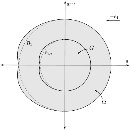
Figure 1. Geometry of $\Omega$ as described in Section 5.

Suppose that $u\in C^{2}(\Omega)\cap L^{\infty}(\mathbb{R}^{n})$ satisfies the torsion problem

$$\left\{\begin{array}[]{r@{ \ }l @{\quad\: \;} l}(-\Delta)^{s}u&=1\hfil\quad\>&\text{in }\Omega,\\ u&=0\hfil\quad\>&\text{in }\mathbb{R}^{n}\setminus\Omega.\end{array}\right.$$

In this case, if $v(x):=u(x)-u(-x_{1},x_{2},\dots,x_{n})$, then $v$ is antisymmetric in $\mathbb{R}^{n}$ with respect to $\{x_{1}=0\}$ and $s$-harmonic in $B_{1}$. Hence, by the Poisson kernel representation, (up to normalization constants)

$$v(x) =\int_{\mathbb{R}^{n}\setminus B_{1}}\bigg{(}\frac{1-|x|^{2}}{|y|^{2}-1}\bigg{)}^{s}\frac{v(y)}{|x-y|^{n}}\mathop{}\!dy.$$

Using the antisymmetry of $v$, we may rewrite this as

$$v(x) =\int_{\mathbb{R}^{n}_{+}\setminus B_{1}^{+}}\bigg{(}\frac{1-|x|^{2}}{|y|^{2}-1}\bigg{)}^{s}\bigg{(}\frac{1}{|x-y|^{n}}-\frac{1}{|x^{\prime}-y|^{n}}\bigg{)}v(y)\mathop{}\!dy$$

$$=\int_{\Omega^{+}\setminus B_{1}^{+}}\bigg{(}\frac{1-|x|^{2}}{|y|^{2}-1}\bigg{)}^{s}\bigg{(}\frac{1}{|x-y|^{n}}-\frac{1}{|x^{\prime}-y|^{n}}\bigg{)}u(y)\mathop{}\!dy,$$

where $x^{\prime}$ denotes the reflection of the point $x$ with respect to $\{x_{1}=0\}$.

Now, by oAZAv7vy, when $[u]_{\partial G}$ is sufficiently small, then $\Omega$ is uniformly close to $B_{1}$, so we can suppose that $G_{\lambda}^{\prime}\subset B_{3/4}$. Therefore, for all $x\in\partial G$ and $y\in\mathbb{R}^{n}_{+}\setminus\Omega$,

$$(1-|x|^{2})^{s}\bigg{(}\frac{1}{|x-y|^{n}}-\frac{1}{|x^{\prime}-y|^{n}}\bigg{)} \geqslant Cx_{1}y_{1}.$$

Also, by Corollary LABEL:zAPw0npM, we have that $u\geqslant C\delta^{s}_{\partial\Omega}$ (with $C>0$ not depending on $u$), and thus

$$v(x) \geqslant Cx_{1}\int_{\Omega^{+}\setminus B_{1}^{+}}\frac{y_{1}u(y)}{(|y|^{2}-1)^{s}}\mathop{}\!dy\geqslant Cx_{1}\int_{\Omega^{+}\setminus B_{1}^{+}}\frac{y_{1}\delta_{\partial\Omega}^{s}(y)}{\delta_{\partial B_{1}}^{s}(y)}\mathop{}\!dy.$$

Recall the discussion on the moving plane method on page 4 and, for simplicity, assume that we are in the first case (the second case can be treated similarly), so there exists $p\in(\partial G\cap\partial G_{\lambda}^{\prime})\setminus\{x_{1}=0\}$. Hence,

(5.1) $$\int_{\Omega^{+}\setminus B_{1}^{+}}y_{1}\bigg{(}\frac{\delta_{\partial\Omega}(y)}{\delta_{\partial B_{1}}(y)}\bigg{)}^{s}\mathop{}\!dy \leqslant C\frac{v(p)}{p_{1}}\leqslant C[u]_{\partial G}.$$

Now the point of obtaining (5.1) is that the left hand side is geometric (does not depend on $u$), and (5.1) is sharp in the sense that the only terms that have been ‘thrown away’ are bounded away from zero as $[u]_{\partial G}\to 0$. This suggests that if $[u]_{\partial G}$ is of order $\varepsilon$ then the behaviour of

$$\int_{\Omega^{+}\setminus B_{1}^{+}}y_{1}\bigg{(}\frac{\delta_{\partial\Omega}(y)}{\delta_{\partial B_{1}}(y)}\bigg{)}^{s}\mathop{}\!dy$$

as a function of $\varepsilon$ will entirely determine the optimal exponent $\overline{\beta}(s)$ (recall that the definition of $\overline{\beta}(s)$ is given after the statement of oAZAv7vy in Section 1). This is surprising, since in the local case, the problem is entirely an interior one in that the proof relies only on interior estimates such as the Harnack inequality while, it appears that in the nonlocal case, the geometry of the boundary may have a significant effect on the value of $\overline{\beta}(s)$. If one hopes to obtain that $\overline{\beta}(s)=1$ from (5.1) then it would be necessary to show that

$$\int_{\Omega^{+}\setminus B_{1}^{+}}y_{1}\bigg{(}\frac{\delta_{\partial\Omega}(y)}{\delta_{\partial B_{1}}(y)}\bigg{)}^{s}\mathop{}\!dy\geqslant C|\Omega\setminus B_{1}^{+}|.$$

If it were true that $y_{1}\delta^{s}_{\partial\Omega}\geqslant C\delta^{s}_{\partial B_{1}}$ then this would follow immediately; however, this is not the case as seen by sending $y\to\partial\mathbb{R}^{n}_{+}\cap B_{1/2}$.

Moreover, even though we made several major assumptions on the geometry of $\Omega$ to obtain (5.1), we believe that the inequality is indicative of the more general situation. Indeed, one would expect that, under reasonable assumptions on $\partial\Omega$, similar estimates to the ones employed above would hold for Poisson kernels in general domains, so one may suspect that an inequality of the form

$$\int_{\Omega\triangle\Omega^{\prime}}\delta_{\pi_{\lambda}}(y)\bigg{(}\frac{\delta_{\partial\Omega}(y)}{\delta_{\partial\Omega^{\prime}}(y)}\bigg{)}^{s}\mathop{}\!dy \leqslant C[u]_{\partial G}$$

should hold. It would be interesting in future articles to further explore this methodology to try obtain improvements on the exponent in oAZAv7vy.

6. Sharp investigation of a technique to improve the stability exponent

In the papers [Cab+18, Cir+18], it was proven that the only open bounded sets whose boundary has constant nonlocal mean curvature are balls. Moreover, in [Cir+18], the method of moving planes was employed to obtain a stability estimate for sets whose boundary has almost constant nonlocal mean curvature. The stability estimate that the authors proved also seems to achieve the optimal exponent of $1$ which is however obtained using the following technical result, see [Cir+18, Proposition 3.1(b)]:

Lemma 6.1.

Z08Q7917 Let $\Omega\subset\mathbb{R}^{n}$ be an open bounded set with $C^{2,\alpha}$ boundary for $\alpha>2s$ and $s\in(0,1/2)$. Let $\pi_{\lambda}$ be the critical hyperplane. Suppose that $\operatorname{dist}(0,\pi_{\lambda})\leqslant 1/8$ and $B_{r}\subset\Omega\subset B_{R}$ with $1/2\leqslant r\leqslant R\leqslant 2$.

Then,

(6.1) $$\Big{|}\big{\{}x\in\Omega\triangle\Omega^{\prime}\text{ s.t. }\operatorname{dist}(x,\pi_{\lambda})\leqslant\gamma\big{\}}\Big{|}\leqslant C(n)\gamma(R-r)$$

for all $0<\gamma\leqslant 1/4$.

Without this result, the exponent in the stability estimate in [Cir+18] would have been $1/2$, so Z08Q7917 seems to play a major role in [Cir+18] in the attempt of “doubling the exponent” that they obtained in previous estimates. This feature is extremely relevant to our main result, oAZAv7vy, since we hoped that a similar argument to Z08Q7917 would lead to an exponent that was twice the one that we obtained. Unfortunately, we believe that, in the very broad generality in which the result is stated in [Cir+18], Z08Q7917 may not be true, and we present a counter-example (which may also impact some of the statements in [Cir+18]) as well as a corrected statement of Z08Q7917.

6.1. A geometric lemma and a counter-example to Z08Q7917

The main result of this section is a geometric lemma which may be viewed as a corrected version of Z08Q7917. Moreover, we will give an explicit family of domains which demonstrate that our geometric lemma is sharp. This family will also serve as a counter-example to Z08Q7917.

An essential component to the geometric lemma that is not present in the assumptions of Z08Q7917 is a uniform bound on the boundary regularity of $\partial\Omega$. To our knowledge, there is no ‘standard’ definition of such a bound, so we will begin by concretely specifying what is meant by this.

Let $\Omega$ be an open subset of $\mathbb{R}^{n}$ with $C^{1}$ boundary. For each $x\in\partial\Omega$, let

$$\Pi_{x}(y):=(y-x)-((y-x)\cdot\nu(x))\nu(x),$$

which is the projection of $\mathbb{R}^{n}$ onto $T_{x}\partial\Omega$, that is, the tangent plane of $\partial\Omega$ at $x$. We have made a translation in the definition of $\Pi_{x}$, so that $\Pi_{x}(x)=0$. For simplicity, we will often identify $T_{x}\partial\Omega$ with $\mathbb{R}^{n-1}$.

Definition 6.2.

deZqwlaB Let $\Omega$ be an open subset of $\mathbb{R}^{n}$ with $C^{\alpha}$ boundary, with $\alpha>1$, and let $\rho$, $M>0$. We say that $\partial\Omega\in C^{\alpha}_{M,\rho}$ if, for all $x\in\partial\Omega$, there exists $\psi^{(x)}:B_{\rho}^{n-1}\to\mathbb{R}$ such that $\psi^{(x)}\in C^{\alpha}(B_{\rho}^{n-1})$, $\|\psi^{(x)}\|_{C^{\alpha}(B_{\rho}^{n-1})}\leqslant M$, and

$$B_{\rho}(x)\cap\Omega=\big{\{}y\in B_{\rho}(x)\text{ s.t. }y\cdot\nu(x)<\psi^{(x)}(\Pi_{x}(y))\big{\}}.$$

We remark that, if $\alpha\in\mathbb{Z}$ in Definition LABEL:deZqwlaB, the notation $C^{\alpha}_{M,\rho}$ means $C^{\alpha-1,1}_{M,\rho}$.

We now give the geometric lemma, the main result of this section.

Theorem 6.3.

m9q9X2hE Let $\Omega\subset\mathbb{R}^{n}$ be an open bounded set with $\partial\Omega\in C^{\alpha}_{M,\rho}$, with $\alpha>1$, for some $M>0$ and $\rho\in(0,1/4)$. Moreover, suppose that $B_{r}\subset\Omega\subset B_{R}$ with $1/2\leqslant r\leqslant R\leqslant 2$. Let $e\in\mathbb{S}^{n-1}$, denote by $\pi_{\lambda}$ the critical hyperplane with respect to $e$, and suppose that $\operatorname{dist}(0,\pi_{\lambda})\leqslant 1/8$.

Then,

(6.2) $$\Big{|}\big{\{}x\in\Omega\triangle\Omega^{\prime}\text{ s.t. }\operatorname{dist}(x,\pi_{\lambda})\leqslant\gamma\big{\}}\Big{|}\leqslant C\gamma(R-r)^{1-\frac{1}{\alpha}}$$

for all $0<\gamma\leqslant 1/4$. The constant $C$ depends only on $n$, $M$, $\rho$, and $\alpha$.

In order to prove Theorem LABEL:m9q9X2hE, we require two preliminary lemmata. The first lemma gives an elementary estimate of the left hand side of (6.2) in terms of $R-r$ and an error term involving $\operatorname{dist}(0,\pi_{\lambda})$.

Lemma 6.4.

o1pUKCHX Let $\Omega\subset\mathbb{R}^{n}$ be an open bounded set with $C^{1}$ boundary, and $B_{r}\subset\Omega\subset B_{R}$ with $1/2\leqslant r\leqslant R\leqslant 2$. Let $e\in\mathbb{S}^{n-1}$, denote by $\pi_{\lambda}$ the critical hyperplane with respect to $e$, and suppose that $\operatorname{dist}(0,\pi_{\lambda})\leqslant 1/8$.

Then,

$$\Big{|}\big{\{}x\in\Omega\triangle\Omega^{\prime}\text{ s.t. }|x_{1}-\lambda|\leqslant\gamma\big{\}}\Big{|}\leqslant C\gamma\big{(}R-r+\gamma|\lambda|\big{)}$$

for all $0<\gamma\leqslant 1/4$. The constant $C$ depends only on $n$.

Proof.

First, observe that

(6.3) $$\Omega\triangle\Omega^{\prime}\subset(B_{R}\cup B_{R}^{\prime})\setminus(B_{r}\cap B_{r}^{\prime})$$

where $B_{\rho}^{\prime}$ is the reflection of $B_{\rho}$ across the critical hyperplane. Indeed, if $x\in\Omega\cup\Omega^{\prime}$ then $x\in\Omega\subset B_{R}$ or $x\in\Omega^{\prime}\subset B_{R}^{\prime}$, so $x\in B_{R}\cup B_{R}^{\prime}$. Moreover, if $x\in B_{r}\cap B_{r}^{\prime}$ then $x\in B_{r}\subset\Omega$ and $x\in B_{r}^{\prime}\subset\Omega^{\prime}$, so $B_{r}\cap B_{r}^{\prime}\subset\Omega\cap\Omega^{\prime}$. Then (6.3) follows from the the fact that $\Omega\triangle\Omega^{\prime}=(\Omega\cup\Omega^{\prime})\setminus(\Omega\cap\Omega^{\prime})$.

From (6.3), it immediately follows that

$$\Big{|}\big{\{}x\in\Omega\triangle\Omega^{\prime}\text{ s.t. }|x_{1}-\lambda|\leqslant\gamma\big{\}}\Big{|} \leqslant\Big{|}\big{\{}x\in(B_{R}\cup B_{R}^{\prime})\setminus(B_{r}\cap B_{r}^{\prime})\text{ s.t. }|x_{1}-\lambda|\leqslant\gamma\big{\}}\Big{|}.$$

Without loss of generality, we may assume that $\lambda>0$. Then

$$\Big{|}\big{\{}x\in(B_{R}\cup B_{R}^{\prime}) \setminus(B_{r}\cap B_{r}^{\prime})\text{ s.t. }|x_{1}-\lambda|\leqslant\gamma\big{\}}\Big{|}$$

$$=2\Big{|}\big{\{}x\in B_{R}\setminus B_{r}^{\prime}\text{ s.t. }\lambda-\gamma<x_{1}<\lambda\big{\}}\Big{|}$$

$$=2\Big{(}\Big{|}B_{R}\cap\{\lambda-\gamma<x_{1}<\lambda\big{\}}\Big{|}-\Big{|}B_{r}^{\prime}\cap\big{\{}\lambda-\gamma<x_{1}<\lambda\big{\}}\Big{|}\Big{)}.$$

Hence, via the co-area formula, we obtain that

$$\Big{|}\big{\{}x\in(B_{R}\cup B_{R}^{\prime}) \setminus(B_{r}\cap B_{r}^{\prime})\text{ s.t. }|x_{1}-\lambda|\leqslant\gamma\big{\}}\Big{|}$$

$$=2\int_{\lambda-\gamma}^{\lambda}\left[\mathcal{H}^{n-1}\left(B_{\sqrt{R^{2}-t^{2}}}^{n-1}\right)-\mathcal{H}^{n-1}\left(B_{\sqrt{r^{2}-(2\lambda-t)^{2}}}^{n-1}\right)\right]\mathop{}\!dt$$

$$=2\omega_{n-1}\int_{\lambda-\gamma}^{\lambda}\left[\big{(}R^{2}-t^{2}\big{)}^{\frac{n-1}{2}}-\big{(}r^{2}-(2\lambda-t)^{2}\big{)}^{\frac{n-1}{2}}\right]\mathop{}\!dt.$$

Next, if $0<a<\tau<b$ then

$$\bigg{|}\frac{\mathop{}\!d}{\mathop{}\!d\tau}\tau^{\frac{n-1}{2}}\bigg{|} =\frac{n-1}{2}\tau^{\frac{n-3}{2}}\leqslant\frac{n-1}{2}\begin{cases}a^{-1/2},&\text{if }n=2\\ b^{\frac{n-3}{2}},&\text{if }n\geqslant 3.\end{cases}$$

Since $\lambda>0$ and $2\lambda-t\in(\lambda,\lambda+\gamma)\subset(0,3/8)$, we have that

$$C^{-1}\leqslant r^{2}-(2\lambda-t)^{2}\leqslant R^{2}-t^{2}\leqslant C\qquad\text{ for all }t\in(\lambda-\gamma,\lambda)$$

with $C>0$ a universal constant. Hence,

$$\Big{|}\big{(}R^{2}-t^{2}\big{)}^{\frac{n-1}{2}}-\big{(}r^{2}-(2\lambda-t)^{2}\big{)}^{\frac{n-1}{2}}\Big{|} \leqslant C\big{|}\big{(}R^{2}-t^{2}\big{)}-\big{(}r^{2}-(2\lambda-t)^{2}\big{)}\big{|}$$

$$\leqslant C\big{(}R-r+\lambda(\lambda-t)\big{)}.$$

Gathering these pieces of information, we conclude that

$$\Big{|}\big{\{}x\in\Omega\triangle\Omega^{\prime}\text{ s.t. }|x_{1}-\lambda|\leqslant\gamma\big{\}}\Big{|} \leqslant C\int_{\lambda-\gamma}^{\lambda}\big{(}R-r+\lambda(\lambda-t)\big{)}\mathop{}\!dt\leqslant C\gamma\big{(}R-r+\gamma\lambda\big{)},$$

as required. ∎

The purpose of the second lemma will be to reduce the proof of m9q9X2hE to the case of graphs of functions.

Lemma 6.5.

GNZAnsDn Let $\Omega\subset\mathbb{R}^{n}$ be an open bounded set with $\partial\Omega\in C^{\alpha}_{M,\rho}$, with $\alpha>1$, for some $M>0$ and $\rho\in(0,1/4)$.

Then, there exists $\varepsilon_{0}\in(0,1)$ such that, for all $\varepsilon\in(0,\varepsilon_{0}]$, it holds that if $B_{1-\varepsilon/2}\subset\Omega\subset B_{1+\varepsilon/2}$ then there exists $\psi_{\varepsilon}:=\psi:B_{3/4}^{n-1}\to(0,+\infty)$ such that $\psi\in C^{\alpha}(B_{3/4}^{n-1})$,

(6.4) $$\big{\|}\psi-\sqrt{1-|x^{\prime}|^{2}}\big{\|}_{C^{1}(B_{3/4}^{n-1})}\leqslant C\varepsilon^{1-\frac{1}{\alpha}},$$

and

(6.5) $$\Omega\cap\big{(}B_{3/4}^{n-1}\times(0,+\infty)\big{)}=\{x\in\mathbb{R}^{n}\text{ s.t. }0<x_{n}<\psi(x^{\prime})\}.$$

The constant $C$ depends only on $n$, $\alpha$, $\rho$, and $M$.

Proof.

Let $x_{\star}\in\partial\Omega\cap\big{(}B_{3/4}^{n-1}\times(0,+\infty)\big{)}$ and $\psi^{(x_{\star})}$ be the function given in deZqwlaB corresponding to the point $x_{\star}$. Next, let $A$ be a rigid motion such that $Ax_{\star}=0$, $T_{x_{\star}}\partial\Omega$ is mapped t  $\mathbb{R}^{n-1}\times\{0\}$, and $\nu(x_{\star})$ is mapped to $e_{n}$. To avoid any confusion, we will always use the variable $x$ to denote points in the original (unrotated) coordinates and $y$ to denote points in the new rotated coordinates, i.e. $y=Ax$. By deZqwlaB, in the $y$ coordinates,

$$y=(y^{\prime},\psi^{(x_{\star})}(y^{\prime}))\qquad\text{ for all }y\in B_{\rho}\cap\partial\Omega$$

where $y^{\prime}=(y_{1},\dots,y_{n-1})$.

Next, if $\partial\Omega$ is contained in the closure of $B_{1+\varepsilon/2}\setminus B_{1-\varepsilon/2}$, we have that

$$\bigg{(}1-\frac{\varepsilon}{2}\bigg{)}^{2}-|y^{\prime}|^{2}\leqslant\big{(}\psi^{(x_{\star})}(y^{\prime})\big{)}^{2}\leqslant\bigg{(}1+\frac{\varepsilon}{2}\bigg{)}^{2}-|y^{\prime}|^{2}$$

for all $y^{\prime}\in B^{n-1}_{\rho}$.

Additionally, by Bernoulli’s inequality, we have that

$$0\leqslant\sqrt{\bigg{(}1+\frac{\varepsilon}{2}\bigg{)}^{2}-|y^{\prime}|^{2}}-\sqrt{1-|y^{\prime}|^{2}} \leqslant\frac{1}{2\sqrt{1-|y^{\prime}|^{2}}}\bigg{(}\varepsilon+\frac{\varepsilon^{2}}{4}\bigg{)}\leqslant C\varepsilon$$

with $C=C(\rho)>0$. Similarly, we also have that

$$-C\varepsilon\leqslant\sqrt{\bigg{(}1-\frac{\varepsilon}{2}\bigg{)}^{2}-|y^{\prime}|^{2}}-\sqrt{1-|y^{\prime}|^{2}}\leqslant 0.$$

Hence, it follows that

$$\big{|}|\psi^{(x_{\star})}(y^{\prime})|-\sqrt{1-|y^{\prime}|^{2}}\big{|} \leqslant C\varepsilon\qquad\text{for all }y^{\prime}\in B^{n-1}_{\rho}.$$

Thus, by interpolation, we have that

$$\big{\|} |\psi^{(x_{\star})}(y^{\prime})|-\sqrt{1-|y^{\prime}|^{2}}\big{\|}_{C^{1}(B^{n-1}_{\rho})}$$

$$\leqslant C\big{\|}|\psi^{(x_{\star})}(y^{\prime})|-\sqrt{1-|y^{\prime}|^{2}}\big{\|}_{C^{\alpha}(B^{n-1}_{\rho})}\big{\|}|\psi^{(x_{\star})}(y^{\prime})|-\sqrt{1-|y^{\prime}|^{2}}\big{\|}_{L^{\infty}(B^{n-1}_{\rho})}^{1-\frac{1}{\alpha}}$$

$$\leqslant C\varepsilon^{1-\frac{1}{\alpha}}$$

using also that $\partial\Omega\in C^{\alpha}_{M,\rho}$.

Note that we have left the $y$ variable in the equations above to emphasise that we are still using the rotated $y$ coordinates. Now, returning to the original $x$ coordinates, we observe that, by the above computation, we have that $\partial\Omega$ is uniformly close to $\partial B_{1}$ in the $C^{1}$ sense, so

$$\nu(x)\cdot e_{n}\geqslant C>0\qquad\text{ for all }x\in\partial\Omega\cap\big{(}B_{3/4}^{n-1}\times(0,+\infty)\big{)}$$

provided that $\varepsilon$ is sufficiently small. Thus, it follows that $\partial\Omega$ is given by a graph with respect to the $e_{n}$ direction, that is, the claim in (6.5) holds for some $\psi:B_{3/4}^{n-1}\to(0,+\infty)$. We can see that $\psi\in C^{\alpha}(B_{3/4}^{n-1})$ since $\partial\Omega$ is $C^{\alpha}$ and we obtain the claim in (6.4) by an identical interpolation argument to the one above. ∎

We may now give the proof of m9q9X2hE.

Proof of m9q9X2hE.

Without loss of generality, we may assume that $e=e_{1}$ and $\lambda>0$. By o1pUKCHX, it is enough to prove that

(6.6) $$\lambda\leqslant C(n,M,\rho,\alpha)(R-r)^{1-\frac{1}{\alpha}}.$$

Since $\lambda\leqslant 2$, if there exists $C=C(n,M,\rho,\alpha)>0$ such that $R-r\geqslant C$ then we are done, so we may assume that $R-r=\varepsilon$ with $\varepsilon$ arbitrarily small. Moreover, by rescaling, we may further assume that $r=1-\varepsilon/2$ and $R=1+\varepsilon/2$. Furthermore, let $\psi:B_{3/4}^{n-1}$ be the function given by GNZAnsDn.

First, let us consider Case 1 of the method of moving planes. In this case, we obtain a point $p=(p_{1},\dots,p_{n})\in(\partial\Omega\cap\partial\Omega^{\prime}_{\lambda})\setminus\pi_{\lambda}$ (recall that, in this notation, $\Omega^{\prime}_{\lambda}=\Omega^{\prime}\cap H_{\lambda}$, so $p_{1}<\lambda$). Hence, we have that $r^{2}\leqslant|p|^{2}\leqslant(r+\varepsilon)^{2}$ and $r^{2}\leqslant|Q_{\pi_{\lambda}}(p)|^{2}\leqslant(r+\varepsilon)^{2}$ (recall that $Q_{\pi_{\lambda}}$ reflects a point across $\pi_{\lambda}$), from which it follows that

$$\lambda(\lambda-p_{1})\leqslant\varepsilon(2r+\varepsilon)\leqslant C\varepsilon.$$

If $\lambda-p_{1}\geqslant 1/4$ then we are done, so we may assume that $\lambda-p_{1}<1/4$.

Moreover, by rotating with respect to $(x_{2},\dots,x_{n})$, we may assume without loss of generality that $p_{2}=\dots=p_{n-1}=0$ and $p_{n}>0$. In particular, this implies that $p^{\prime}=(p_{1},\dots,p_{n-1})\in B_{3/4}^{n-1}$.

Now, on one hand, if $\psi_{\lambda}(x^{\prime}):=\psi(x^{\prime})-\psi(2\lambda-x_{1},x_{2},\dots,x_{n-1})$ then $\psi_{\lambda}\geqslant 0$ for $x^{\prime}\in B_{3/4}^{n-1}\cap\{x_{1}<\lambda\}$ and $\psi_{\lambda}(p^{\prime})=0$, so $\partial_{1}\psi_{\lambda}(p^{\prime})=0$. On the other hand, by GNZAnsDn, if $x^{\prime\prime}=(x_{2},\dots,x_{n-1})$,

$$\partial_{1}\psi_{\lambda}(p^{\prime}) =\partial_{1}\big{(}\psi_{\lambda}-\sqrt{1-|x^{\prime}|^{2}}+\sqrt{1-(2\lambda-x_{1})^{2}-|x^{\prime\prime}|^{2}}\big{)}(p^{\prime})$$

$$\qquad+\partial_{1}\big{(}\sqrt{1-|x^{\prime}|^{2}}-\sqrt{1-(2\lambda-x_{1})^{2}-|x^{\prime\prime}|^{2}}\big{)}(p^{\prime})$$

$$\leqslant C\varepsilon^{1-\frac{1}{\alpha}}-\bigg{(}\frac{p_{1}}{\sqrt{1-p_{1}^{2}}}+\frac{2\lambda-p_{1}}{\sqrt{1-(2\lambda-p_{1})^{2}}}\bigg{)}.$$

Hence, we have that

(6.7) $$\frac{p_{1}}{\sqrt{1-p_{1}^{2}}}+\frac{2\lambda-p_{1}}{\sqrt{1-(2\lambda-p_{1})^{2}}}\leqslant C\varepsilon^{1-\frac{1}{\alpha}}.$$

Moreover, we claim that

(6.8) $$\frac{p_{1}}{\sqrt{1-p_{1}^{2}}}+\frac{2\lambda-p_{1}}{\sqrt{1-(2\lambda-p_{1})^{2}}}\geqslant\frac{2\lambda}{\sqrt{1-\lambda^{2}}}.$$

To prove this, we consider the function

$$f(t):=\frac{\lambda-t}{\sqrt{1-(\lambda-t)^{2}}}+\frac{\lambda+t}{\sqrt{1-(\lambda+t)^{2}}}$$

for $t\in\left(-\frac{1}{2},\frac{1}{2}\right)$. Notice that $f$ is even, and therefore we restrict our analysis to the interval $\left[0,\frac{1}{2}\right)$.

By a direct calculation,

$$f^{\prime}(t) = -\frac{(\lambda-t)^{2}}{(1-(\lambda-t)^{2})^{3/2}}-\frac{1}{\sqrt{1-(\lambda-t)^{2}}}+\frac{1}{\sqrt{1-(\lambda+t)^{2}}}+\frac{(\lambda+t)^{2}}{(1-(\lambda+t)^{2})^{3/2}}$$

$$= -\frac{1}{(1-(\lambda-t)^{2})^{3/2}}+\frac{1}{(1-(\lambda+t)^{2})^{3/2}}.$$

Now we define $\phi(\tau):=(1-\tau)^{-3/2}$. Since $(\lambda-t)^{2}\leqslant(\lambda+t)^{2}\leqslant 17/32<1$, we can write

$$f^{\prime}(t)=\int_{(\lambda-t)^{2}}^{(\lambda+t)^{2}}\phi^{\prime}(\tau)\,d\tau=\frac{3}{2}\int_{(\lambda-t)^{2}}^{(\lambda+t)^{2}}(1-\tau)^{-5/2}\,d\tau\geqslant 0.$$

Therefore, for all $t\in\left(0,\frac{1}{2}\right)$ (and thus for all $t\in\left(-\frac{1}{2},\frac{1}{2}\right)$), we have that

$$f(t)\geqslant f(0)=\frac{2\lambda}{\sqrt{1-\lambda^{2}}}.$$

Hence, setting $t=\lambda-p_{1}\in\left(-\frac{1}{2},\frac{1}{2}\right)$, we obtain the desired inequality in (6.8).

In particular, from (6.8) we have that

$$\frac{p_{1}}{\sqrt{1-p_{1}^{2}}}+\frac{2\lambda-p_{1}}{\sqrt{1-(2\lambda-p_{1})^{2}}}\geqslant C\lambda,$$

for some $C>0$. Putting together this and (6.7), we deduce that the claim in (6.6) holds.

For Case 2 of the method of moving planes, we obtain a point $p\in\partial\Omega\cap\pi_{\lambda}$ at which $\partial\Omega$ is orthogonal to $\pi_{\lambda}$. In this case, we have that $\partial_{1}\psi_{\lambda}(p^{\prime})\geqslant 0$. From here the proof is identical to Case 1. ∎

We will now give an explicit family of domains which demonstrate that the result obtained in m9q9X2hE is sharp. This also serves as a counter-example to Z08Q7917.

Theorem 6.6.

There exists a smooth $1$-parameter family $\{\Omega_{\varepsilon}\}$ of open bounded subsets of $\mathbb{R}^{2}$ such that

• $\partial\Omega_{\varepsilon}\in C^{\alpha}_{M,1/8}$, with $\alpha>1$, for some $M>0$ independent of $\varepsilon$;

• $B_{1-C_{1}\varepsilon}\subset\Omega_{\varepsilon}\subset B_{1+C_{1}\varepsilon}$ for a universal constant $C_{1}>0$;

• if $\pi_{\lambda}$ is the critical hyperplane with respect to $e_{1}$ and $\gamma\in(0,1/4)$, then

  (6.9) $$\Big{|}\big{\{}x\in\Omega_{\varepsilon}\triangle\Omega_{\varepsilon}^{\prime}\text{ s.t. }\operatorname{dist}(x,\pi_{\lambda})\leqslant\gamma\big{\}}\Big{|}\geqslant C_{2}\varepsilon^{1-\frac{1}{\alpha}}$$

  as $\varepsilon\to 0^{+}$. The constant $C_{2}>0$ depends on $n$ and $\gamma$.

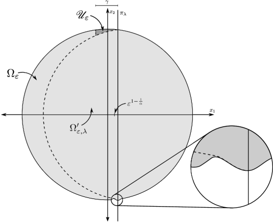
Figure 2. Diagram of $\Omega_{\varepsilon}$ in Theorem 6.6.

Proof.

We will define $\Omega_{\varepsilon}$ by specifying its boundary, see Figure 2. More precisely, in the region $\mathbb{R}^{2}\setminus\big{(}(0,1/2)\times(-3/2,-1/2)\big{)}$, let $\partial\Omega_{\varepsilon}=\partial B_{1}$. For the definition of $\partial\Omega_{\varepsilon}$ in $(0,1/2)\times(-3/2,-1/2)$, let $\eta~{}\in C^{\infty}_{0}(\mathbb{R})$ be such that

$$\begin{cases}\eta(\tau)=2\tau&\text{in }(-1/4,1/4),\\ \eta=0&\text{in }\mathbb{R}\setminus(-1,1),\\ \eta(-\tau)=-\eta(\tau)&\text{in }\mathbb{R},\\ |\eta|\leqslant 1&\text{in }\mathbb{R}.\end{cases}$$

Let also

$$\eta_{\varepsilon}(\tau):=\varepsilon\eta\left(\frac{\tau-\varepsilon^{1-\frac{1}{\alpha}}}{\varepsilon^{1/\alpha}}\right)\qquad{\mbox{and}}\qquad\psi_{\varepsilon}(\tau):=-\sqrt{1-\tau^{2}}-\eta_{\varepsilon}(\tau)$$

and define the remaining portion of $\partial\Omega_{\varepsilon}$ by

$$\partial\Omega_{\varepsilon}\cap\Big{(}(0,1/2)\times(-3/2,-1/2)\Big{)}=\big{\{}(x,\psi_{\varepsilon}(x))\text{ s.t. }x\in(0,1/2)\big{\}}.$$

We observe that $\partial\Omega_{\varepsilon}$ is smooth and that

$$\tau^{2}+(\psi_{\varepsilon}(\tau))^{2} =1+2\eta_{\varepsilon}(\tau)\sqrt{1-\tau^{2}}+(\eta_{\varepsilon}(\tau))^{2}\leqslant 1+C\varepsilon.$$

Hence, by Bernoulli’s inequality,

$$\sqrt{\tau^{2}+\psi_{\varepsilon}(\tau)^{2}}-1 \leqslant C\varepsilon,$$

and similarly, we can show that $\sqrt{\tau^{2}+\psi_{\varepsilon}(\tau)^{2}}-1\geqslant-C\varepsilon$, so $B_{1-C\varepsilon}\subset\Omega_{\varepsilon}\subset B_{1+C\varepsilon}$. Moreover, we have that $\|\psi_{\varepsilon}\|_{C^{\alpha}((0,1/2))}\leqslant M$ for some $M>0$ sufficiently large and independent of $\varepsilon$, so $\partial\Omega_{\varepsilon}\in C^{\alpha}_{M,1/8}$.

Now all that is left to be shown is (6.9). First, we claim that the critical parameter $\lambda_{\varepsilon}$ satisfies

(6.10) $$\lambda_{\varepsilon}\geqslant\varepsilon^{1-\frac{1}{\alpha}}.$$

To prove this, for all $\mu\in\mathbb{R}$, we define $\psi_{\varepsilon,\mu}(\tau):=\psi_{\varepsilon}(\tau)-\psi_{\varepsilon}(2\mu-\tau)$. Furthermore, we consider

$$\tau_{\varepsilon}:=\varepsilon^{1-\frac{1}{\alpha}}-\frac{1}{4}\varepsilon^{\frac{1}{\alpha}}\qquad{\mbox{and}}\qquad\mu_{\varepsilon}:=\varepsilon^{1-\frac{1}{\alpha}}.$$

We have that

$$\psi_{\varepsilon,\mu_{\varepsilon}}(\tau_{\varepsilon}) = -\Big{(}\sqrt{1-\tau_{\varepsilon}^{2}}-\sqrt{1-(2\mu_{\varepsilon}-\tau_{\varepsilon})^{2}}\Big{)}-\varepsilon\left(\eta\left(\frac{\tau_{\varepsilon}-\varepsilon^{1-\frac{1}{\alpha}}}{\varepsilon^{1/\alpha}}\right)-\eta\left(\frac{2\mu_{\varepsilon}-\tau_{\varepsilon}-\varepsilon^{1-\frac{1}{\alpha}}}{\varepsilon^{1/\alpha}}\right)\right)$$

$$= -\Big{(}\sqrt{1-\tau_{\varepsilon}^{2}}-\sqrt{1-(2\mu_{\varepsilon}-\tau_{\varepsilon})^{2}}\Big{)}-2\varepsilon\bigg{(}\frac{\tau_{\varepsilon}-\varepsilon^{1-\frac{1}{\alpha}}}{\varepsilon^{1/\alpha}}-\frac{2\mu_{\varepsilon}-\tau_{\varepsilon}-\varepsilon^{1-\frac{1}{\alpha}}}{\varepsilon^{1/\alpha}}\bigg{)}$$

$$= -\frac{4\mu_{\varepsilon}(\mu_{\varepsilon}-\tau_{\varepsilon})}{\sqrt{1-\tau_{\varepsilon}^{2}}+\sqrt{1-(2\mu_{\varepsilon}-\tau_{\varepsilon})^{2}}}+4\varepsilon^{1-\frac{1}{\alpha}}\big{(}\mu_{\varepsilon}-\tau_{\varepsilon}\big{)}$$

$$= -4\mu_{\varepsilon}(\mu_{\varepsilon}-\tau_{\varepsilon})\left(\frac{1}{2}+o(1)\right)+4\varepsilon^{1-\frac{1}{\alpha}}\big{(}\mu_{\varepsilon}-\tau_{\varepsilon}\big{)}$$

$$= 2\varepsilon^{1-\frac{1}{\alpha}}\big{(}\mu_{\varepsilon}-\tau_{\varepsilon}\big{)}+o\Big{(}\varepsilon^{1-\frac{1}{\alpha}}\big{(}\mu_{\varepsilon}-\tau_{\varepsilon}\big{)}\Big{)}$$

$$= \frac{1}{2}\varepsilon+o(\varepsilon)$$

$$\geqslant \frac{1}{4}\varepsilon,$$

as soon as $\varepsilon$ is sufficiently small.

Hence, we have that $\psi_{\varepsilon,\mu_{\varepsilon}}(\tau_{\varepsilon})>0$, which implies that the reflected region of $\Omega_{\varepsilon,\mu}$ must have left the region $\Omega_{\varepsilon}$ by the time we have reached $\mu=\mu_{\varepsilon}$, so we conclude that the critical time $\lambda_{\varepsilon}$ satisfies $\lambda_{\varepsilon}>\mu_{\varepsilon}$, which gives (6.10).

In fact, since $\eta$ is zero outside of $(-1,1)$, it follows that

$$\lambda_{\varepsilon}\leqslant C\varepsilon^{1-\frac{1}{\alpha}},$$

so, in particular, $\lambda_{\varepsilon}\to 0$ as $\varepsilon\to 0^{+}$.

Finally, to complete the proof of (6.9), we will show that

(6.11) $$\Big{|}\big{\{}x\in\Omega_{\varepsilon}\triangle\Omega_{\varepsilon}^{\prime}\text{ s.t. }\operatorname{dist}(x,\pi_{\lambda})\leqslant\gamma\big{\}}\Big{|}\geqslant C\lambda_{\varepsilon}.$$

Indeed, let $\mathscr{U}_{\varepsilon}:=\big{(}\big{(}\Omega_{\varepsilon}\cap\{\lambda-\gamma<x_{1}<\lambda\}\big{)}\setminus\Omega_{\varepsilon,\lambda}^{\prime}\big{)}\cap\{x_{2}>0\}$, see Figure 2. Observe that

$$\Big{|}\big{(}\Omega_{\varepsilon}\cap\{\lambda-\gamma<x_{1}<\lambda\}\big{)}\setminus\Omega_{\varepsilon,\lambda}^{\prime}\Big{|}\geqslant|\mathscr{U}_{\varepsilon}|.$$

Moreover, using that $\lambda_{\varepsilon}\to 0$, we have that

$$|\mathscr{U}_{\varepsilon}| = \int_{\lambda_{\varepsilon}-\gamma}^{\lambda_{\varepsilon}}\Big{(}\sqrt{1-\tau^{2}}-\sqrt{1-(2\lambda_{\varepsilon}-\tau)^{2}}\Big{)}\mathop{}\!d\tau$$

$$= \int_{\lambda_{\varepsilon}-\gamma}^{\lambda_{\varepsilon}}\frac{4\lambda_{\varepsilon}(\lambda_{\varepsilon}-\gamma)}{\sqrt{1-\tau^{2}}+\sqrt{1-(2\lambda_{\varepsilon}-\tau)^{2}}}\mathop{}\!d\tau$$

$$\geqslant 4\lambda_{\varepsilon}\int_{\lambda_{\varepsilon}-\gamma}^{\lambda_{\varepsilon}-\frac{\gamma}{2}}\frac{\lambda_{\varepsilon}-\gamma}{2}\mathop{}\!d\tau$$

$$\geqslant \frac{\gamma^{2}}{2}\lambda_{\varepsilon},$$

which establishes (6.11), and thus completes the proof of Theorem 6.6. ∎

6.2. An application of m9q9X2hE: improvement of the exponent in oAZAv7vy

We will now show how to use m9q9X2hE to improve the stability exponent in m9q9X2hE. The key step is to use m9q9X2hE to achieve the following modified version of 7TQmUHhl.

Proposition 6.7.

Prop:new per improvement Let $\Omega$ be an open bounded set with $C^{1}$ boundary and satisfying the uniform interior ball condition with radius $r_{\Omega}>0$ and $G$ be an open bounded set with $C^{1}$ boundary such that $\Omega=G+B_{R}$ for some $R>0$. Let $f\in C^{0,1}_{\mathrm{loc}}(\mathbb{R})$ be such that $f(0)\geqslant 0$ and $u$ satisfies (1.8) in the weak sense.

For $e\in\mathbb{S}^{n-1}$, let $\Omega^{\prime}$ denote the reflection of $\Omega$ with respect to the critical hyperplane $\pi_{\lambda}$.

In addition, suppose that $\partial\Omega\in C^{\alpha}_{M,\rho}$, with $\alpha>1$, for some $M>0$ and $\rho\in(0,1/4)$, and that

(6.12) $$B_{\rho_{i}}\subset\Omega\subset B_{\rho_{e}}\quad\text{ with }\quad\frac{1}{2}\leqslant\rho_{i}\leqslant\rho_{e}\leqslant 2$$

and

(6.13) $$\rho_{e}-\rho_{i}\geqslant 4^{\frac{\alpha(s+2)}{(\alpha-1)(s+1)}}[u]_{\partial G}^{\frac{\alpha}{(\alpha-1)(s+1)}}.$$

Then,

$$|\Omega\triangle\Omega^{\prime}|\leqslant\widetilde{C}_{\star}(\rho_{e}-\rho_{i})^{\frac{\alpha-1}{\alpha(s+2)}}\,[u]_{\partial G}^{\frac{1}{s+2}},$$

where $\widetilde{C}_{\star}$ is some explicit constant depending on $n$, $s$, $\alpha$, $M$, $\rho$, $\operatorname{diam}\Omega$, $R$, $[f]_{C^{0,1}([0,\|u\|_{L^{\infty}(\Omega)}])}$, and $\|u\|_{L_{s}(\mathbb{R}^{n})}$.

Proof.

The proof of Proposition LABEL:Prop:new_per_improvement is a suitable modification of the one of 7TQmUHhl. More precisely, we recall (4.8) and we use that $f(0)\geqslant 0$ to obtain that

(6.14) $$\begin{split}\Big{|}\big{\{}x\in(\Omega\cap H_{\lambda}^{\prime})\setminus\Omega_{\lambda}^{\prime}\text{ s.t. }x_{1}\delta_{\partial\Omega}^{s}(x)>\gamma\big{\}}\Big{|}\leqslant\;&\frac{CC_{\ast}^{-1}\big{(}f(0)+\|u\|_{L_{s}(\mathbb{R}^{n})}\big{)}^{-1}}{\gamma}[u]_{\partial G}\\ \leqslant\;&\frac{CC_{\ast}^{-1}\|u\|_{L_{s}(\mathbb{R}^{n})}^{-1}}{\gamma}[u]_{\partial G},\end{split}$$

where $C_{\ast}$ is as in zAPw0npM.

Furthermore, given $\gamma$, $\beta\in\left(0,\frac{1}{4}\right]$, we see that

$$\Big{|}\big{\{}x\in(\Omega\cap H_{\lambda}^{\prime})\setminus\Omega_{\lambda}^{\prime}\text{ s.t. }x_{1}\delta_{\partial\Omega}^{s}(x)\leqslant\gamma\big{\}}\Big{|}$$

$$= \Big{|}\big{\{}x\in(\Omega\cap H_{\lambda}^{\prime})\setminus\Omega_{\lambda}^{\prime}\text{ s.t. }x_{1}\delta_{\partial\Omega}^{s}(x)\leqslant\gamma,x_{1}<\beta\big{\}}\Big{|}$$

$$\qquad+\Big{|}\big{\{}x\in(\Omega\cap H_{\lambda}^{\prime})\setminus\Omega_{\lambda}^{\prime}\text{ s.t. }x_{1}\delta_{\partial\Omega}^{s}(x)\leqslant\gamma,x_{1}\geqslant\beta\big{\}}\Big{|}$$

$$\leqslant \Big{|}\big{\{}x\in\Omega^{+}\text{ s.t. }x_{1}<\beta\big{\}}\Big{|}+\left|\left\{x\in\Omega\text{ s.t. }\delta_{\partial\Omega}(x)\leqslant\left(\frac{\gamma}{\beta}\right)^{\frac{1}{s}}\right\}\right|.$$

Now, using m9q9X2hE we have that

$$\Big{|}\big{\{}x\in\Omega^{+}\text{ s.t. }x_{1}<\beta\big{\}}\Big{|} \leqslant C\,(\rho_{e}-\rho_{i})^{1-\frac{1}{\alpha}}\beta,$$

for some $C>0$ depending only on $n$, $M$, $\rho$ and $\alpha$.

Also, using [Cir+23, Lemma 5.2] and [Tam76], we obtain that

$$\left|\left\{x\in\Omega\text{ s.t. }\delta_{\partial\Omega}(x)\leqslant\left(\frac{\gamma}{\beta}\right)^{\frac{1}{s}}\right\}\right| \leqslant\frac{2n|\Omega|}{r_{\Omega}}\left(\frac{\gamma}{\beta}\right)^{\frac{1}{s}}.$$

Gathering these pieces of information, we obtain that

$$\Big{|}\big{\{}x\in(\Omega\cap H_{\lambda}^{\prime})\setminus\Omega_{\lambda}^{\prime}\text{ s.t. }x_{1}\delta_{\partial\Omega}^{s}(x)\leqslant\gamma\big{\}}\Big{|}\leqslant C(\rho_{e}-\rho_{i})^{1-\frac{1}{\alpha}}\beta+\frac{2n|\Omega|}{r_{\Omega}}\left(\frac{\gamma}{\beta}\right)^{\frac{1}{s}}.$$

From this and (6.14), we now deduce that

$$|\Omega\triangle\Omega^{\prime}| = 2|(\Omega\cap H_{\lambda}^{\prime})\setminus\Omega^{\prime}_{\lambda}|$$

$$\leqslant CC_{\ast}^{-1}\|u\|_{L_{s}(\mathbb{R}^{n})}^{-1}\frac{[u]_{\partial G}}{\gamma}+C(\rho_{e}-\rho_{i})^{1-\frac{1}{\alpha}}\beta+\frac{2n|\Omega|}{r_{\Omega}}\left(\frac{\gamma}{\beta}\right)^{\frac{1}{s}}$$

$$\leqslant C\left[\frac{[u]_{\partial G}}{\gamma}+(\rho_{e}-\rho_{i})^{1-\frac{1}{\alpha}}\beta+\left(\frac{\gamma}{\beta}\right)^{\frac{1}{s}}\right].$$

Minimizing the expression in the last line in the variables $(\beta,\gamma)$ gives

$$\gamma\beta=\frac{[u]_{\partial G}}{(\rho_{e}-\rho_{i})^{1-\frac{1}{\alpha}}}\qquad{\mbox{ and }}\qquad\beta=\frac{[u]_{\partial G}^{\frac{1}{s+2}}}{(\rho_{e}-\rho_{i})^{{\frac{(\alpha-1)(s+1)}{\alpha(s+2)}}}},$$

that is,

$$\gamma=\frac{[u]_{\partial G}^{\frac{s+1}{s+2}}}{(\rho_{e}-\rho_{i})^{\frac{\alpha-1}{\alpha(s+2)}}}\qquad{\mbox{ and }}\qquad\beta=\frac{[u]_{\partial G}^{\frac{1}{s+2}}}{(\rho_{e}-\rho_{i})^{{\frac{(\alpha-1)(s+1)}{\alpha(s+2)}}}}.$$

Notice that the assumption in (6.13) guarantees that, with these choices, $\gamma$, $\beta\in\left(0,\frac{1}{4}\right]$.

Thus, we conclude that

$$|\Omega\triangle\Omega^{\prime}|\leqslant C\,(\rho_{e}-\rho_{i})^{\frac{\alpha-1}{\alpha(s+2)}}\,[u]_{\partial G}^{\frac{1}{s+2}}.$$

This completes the proof of Proposition LABEL:Prop:new_per_improvement. ∎

Proposition LABEL:Prop:new_per_improvement leads to the following statement, which is the counterpart of Proposition LABEL:k4VRS3Fx.

Proposition 6.8.

k4VRS3FxBIS Let $\Omega$ be an open bounded set with $C^{1}$ boundary and satisfying the uniform interior ball condition with radius $r_{\Omega}>0$ and suppose that the critical planes $\pi_{e_{i}}$ with respect to the coordinate directions $e_{i}$ coincide with $\{x_{i}=0\}$ for every $i=1,\dots,n$. Also, given $e\in\mathbb{S}^{n-1}$, denote by $\lambda_{e}$ the critical value associated with $e$ as in (4.1).

In addition, suppose that $\partial\Omega\in C^{\alpha}_{M,\rho}$, with $\alpha>1$, for some $M>0$ and $\rho\in(0,1/4)$, and that the assumptions in (6.12) and (6.13) are satisfied.

Assume that

$$[u]^{\frac{1}{s+2}}_{\partial G}\leqslant\frac{|\Omega|}{n\widetilde{C}_{\star}}$$

where $\widetilde{C}_{\star}$ is the constant in Proposition LABEL:Prop:new_per_improvement.

Then,

$$|\lambda_{e}|\leqslant C\,(\rho_{e}-\rho_{i})^{\frac{\alpha-1}{\alpha(s+2)}}[u]_{\partial G}^{\frac{1}{s+2}}$$

for all $e\in\mathbb{S}^{n-1}$, where $C$ is some explicit constant depending on $n$, $s$, $\alpha$, $M$, $\rho$, $\operatorname{diam}\Omega$, $R$, $[f]_{C^{0,1}([0,\|u\|_{L^{\infty}(\Omega)}])}$, and $\|u\|_{L_{s}(\mathbb{R}^{n})}$.

We omit the proof of Proposition LABEL:k4VRS3FxBIS, since it follows the same line as that of Proposition LABEL:k4VRS3Fx.

Now, up to a translation, we can suppose that the critical planes $\pi_{e_{i}}$ with respect to the coordinate directions $e_{i}$ coincide with $\{x_{i}=0\}$ for every $i=1,\dots,n$. Hence, following [Cir+18, Proof of Theorem 1.2], we can define

(6.15) $$\rho_{e}:=\max_{\partial\Omega}|x|\qquad{\mbox{ and }}\qquad\rho_{i}:=\min_{\partial\Omega}|x|,$$

and work with $\rho_{e}-\rho_{i}$ (which clearly gives an upper bound for $\rho(\Omega)$) to achieve the desired stability estimates.

In the following result, we also assume that

(6.16) $$\rho_{e}=1.$$

Notice that such an assumption is always satisfied, up to a dilation.

Theorem 6.9.

thm:improvement Let $G$ be an open bounded subset of $\mathbb{R}^{n}$ and $\Omega=G+B_{R}$ for some $R>0$. Furthermore, let $\Omega$ and $G$ have $C^{1}$ boundary, and let $f\in C^{0,1}_{\mathrm{loc}}(\mathbb{R})$ be such that $f(0)\geqslant 0$. Suppose that $u$ satisfies (1.8) in the weak sense.

In addition, let $\partial\Omega\in C^{\alpha}_{M,\rho}$, with $\alpha>1$, for some $M>0$ and $\rho\in(0,1/4)$.

Let $\rho_{e}$ and $\rho_{i}$ be as in (6.15) and (6.16).

Then,

$$\rho(\Omega)\leqslant\rho_{e}-\rho_{i} \leqslant\widetilde{C}[u]_{\partial G}^{\frac{\alpha}{1+\alpha(s+1)}},$$

where $\widetilde{C}$ is some explicit constant depending on $n$, $s$, $\alpha$, $M$, $\rho$, $\operatorname{diam}\Omega$, $R$, $[f]_{C^{0,1}([0,\|u\|_{L^{\infty}(\Omega)}])}$, and $\|u\|_{L_{s}(\mathbb{R}^{n})}$.

Proof.

Without loss of generality, we can assume that (6.13) is satisfied, as otherwise thm:improvement trivially holds.

An inspection of the proof of oAZAv7vy shows that $\rho_{e}$ and $\rho_{i}$ defined in (6.15) satisfy

$$\rho_{e}-\rho_{i} \leqslant C[u]_{\partial G}^{\frac{1}{s+2}}.$$

Thus, if $[u]_{\partial G}\leqslant(2C)^{-(s+2)}$, we obtain that $\rho_{e}-\rho_{i}\leqslant 1/2$, and therefore, in light of the assumption in (6.16), we have that $1/2\leqslant\rho_{i}\leqslant\rho_{e}\leqslant 2$, namely (6.12) is satisfied.

Hence, we can employ Proposition LABEL:k4VRS3FxBIS and obtain that

(6.17) $$|\lambda_{e}|\leqslant C\,(\rho_{e}-\rho_{i})^{\frac{\alpha-1}{\alpha(s+2)}}[u]_{\partial G}^{\frac{1}{s+2}}.$$

The desired result follows by reasoning as in the proof of oAZAv7vy, but using (6.17) instead of (4.11). ∎

7. The exponent for a family of ellipsoids

Throughout this section, we will denote a point $x=(x_{1},\dots,x_{n})\in\mathbb{R}^{n}$ by $x=(x_{1},x^{\prime})$ where $x^{\prime}=(x_{2},\dots,x_{n})\in\mathbb{R}^{n-1}$.

Proposition 7.1.

0LlyfQlx Suppose that $n\geqslant 2$ is an integer, $s\in(0,1)$, and $\varepsilon>0$. Define

(7.1) $$\Omega_{\varepsilon}:=\bigg{\{}(x_{1},x^{\prime})\in\mathbb{R}^{n}\text{ s.t. }\frac{x_{1}^{2}}{(1+\varepsilon)^{2}}+|x^{\prime}|^{2}<1\bigg{\}}.$$

Then, for $0<\varepsilon<1/4$, there exists a 1-parameter family $G_{\varepsilon}\subset\Omega_{\varepsilon}$ with smooth boundary such that

$$G_{\varepsilon}+B_{1/2}=\Omega_{\varepsilon}.$$

Moreover, let $u_{\varepsilon}\in C^{2}(\Omega_{\varepsilon})\cap C^{s}(\mathbb{R}^{n})$ be the unique solution to

(7.4) $$\left\{\begin{array}[]{r@{ \ }l @{\quad\: \;} l}(-\Delta)^{s}u_{\varepsilon}&=1\hfil\quad\>&\text{in }\Omega_{\varepsilon},\\ u_{\varepsilon}&=0\hfil\quad\>&\text{in }\mathbb{R}^{n}\setminus\Omega_{\varepsilon}.\end{array}\right.$$

Then,

(7.5) $$\lim_{\varepsilon\to 0^{+}}\frac{[u_{\varepsilon}]_{\partial G_{\varepsilon}}}{\rho(\Omega_{\varepsilon})} =s\gamma_{n,s}\bigg{(}\frac{3}{4}\bigg{)}^{s-1},$$

where

(7.6) $$\gamma_{n,s}:=\frac{2^{-2s}\Gamma\big{(}\frac{n}{2}\big{)}}{\Gamma\left(\frac{n+2s}{2}\right)\Gamma(1+s)}.$$

The existence of the 1-parameter family $G_{\varepsilon}$ as in 0LlyfQlx is an easy corollary of the following geometric lemma.

Lemma 7.2.

jUJs9Upe Let $n\geqslant 2$ be an integer and suppose that $\Omega$ is an open bounded subset of $\mathbb{R}^{n}$ that satisfies the uniform interior ball condition with radius $r_{\Omega}>0$. If $\delta:\Omega\to\mathbb{R}$ is the distance to the boundary of $\Omega$ and $\Omega^{\rho}:=\{x\in\Omega\text{ s.t. }\delta(x)>\rho\}$ then for all $\rho\in(0,r_{\Omega})$,

$$\Omega^{\rho}+B_{\rho}=\Omega.$$

Moreover, if the boundary of $\Omega$ is $C^{k}$ for some integer $k\geqslant 2$ then, for all $\rho\in(0,r_{\Omega})$, the boundary of $\Omega^{\rho}$ is also $C^{k}$.

Proof.

We will begin by showing that $\Omega^{\rho}+B_{\rho}\subset\Omega$. If $z\in\Omega^{\rho}+B_{\rho}$ then $z=x+y$ for some $x\in\Omega^{\rho}$ and $y\in B_{\rho}$. Let $R>0$ be the largest value possible such that $B_{R}(x)\subset\Omega$. Then $R=\delta(x)$, so $R>\rho$. Hence,

$$|z-x|=|y|<\rho<R,$$

so $z\in B_{R}(x)\subset\Omega$.

Now, let us show that $\Omega\subset\Omega^{\rho}+B_{\rho}$. Let $z\in\Omega$. If $z\in\Omega^{\rho}$ then $z=z+0\in\Omega^{\rho}+B_{\rho}$ and we are done, so we may assume that $z\in\Omega\setminus\Omega^{\rho}$. Now, let $R>0$ be the largest value possible such that $B_{R}(z)\subset\Omega$ and let $p\in\partial\Omega$ be a point at which $B_{R}(z)$ touches $\partial\Omega$. Define the unit vector

$$\nu(p):=\frac{p-z}{|p-z|}.$$

Next, since $B_{R}(z)$ is an interior touching ball, there exists some $\bar{z}\in\Omega$ such that $B_{r_{\Omega}}(\bar{z})$ also touches $\partial\Omega$ at $p$ and $p$, $z$, and $\bar{z}$ are collinear. Now, let $\mu\in(0,\min\{r_{\Omega}-\rho,R\})$ and define

$$x:=z-(\rho-R+\mu)\nu(p).$$

Since $z=\bar{z}+(r_{\Omega}-R)\nu(p)$, it follows that $|x-\bar{z}|=|r_{\Omega}-\rho-\mu|<r_{\Omega}$, so $x\in B_{r_{\Omega}}(\bar{z})$. Hence, $x\in\Omega$. Moreover, $|x-p|=\rho+\mu>\rho$, so $x\in\Omega^{\rho}$ and $|z-x|=\rho-R+\mu<\rho$, so $z-x\in B_{\rho}$. Thus, we have that $z=x+(z-x)\in\Omega^{\rho}+B_{\rho}$ as required. This completes the first part of the proof.

The fact that the boundary of $\Omega^{\rho}$ is $C^{k}$ for any $\rho\in(0,r_{\Omega})$ is a simple consequence of [GT01, Lemma 14.16]. Indeed, following the proof of [GT01, Lemma 14.16], we see that $\delta\in C^{k}(\Gamma^{r_{\Omega}})$ where

$$\Gamma^{r_{\Omega}}:=\{x\in\Omega\text{ s.t. }\delta(x)<r_{\Omega}\}.$$

Then the boundary of $\Omega^{\rho}$ is simply the level set $\Omega\cap\{\delta=\rho\}$ which is contained in $\Gamma^{r_{\Omega}}$, so $\partial\Omega^{\rho}$ is $C^{k}$. ∎

From jUJs9Upe, we immediately obtain the proof of the first part of 0LlyfQlx:

Corollary 7.3.

FOHX1qV4 Suppose that $n\geqslant 2$ is an integer, $s\in(0,1)$, $\varepsilon>0$, and $\Omega_{\varepsilon}$ be as in (7.1).

Then, for $0<\varepsilon<1/4$, there exists a 1-parameter family $G_{\varepsilon}\subset\Omega_{\varepsilon}$ with smooth boundary such that

$$G_{\varepsilon}+B_{1/2}=\Omega_{\varepsilon}.$$

Proof.

It is easy to check that $\Omega_{\varepsilon}$ satisfies the uniform interior ball condition with uniform radius given by $r_{\Omega_{\varepsilon}}=(1+\varepsilon)^{-1}$. Hence, since $\varepsilon<1/4$, we have that $r_{\Omega_{\varepsilon}}>1/2$, so if $G_{\varepsilon}:=\Omega_{\varepsilon}^{\rho}$ with $\rho=1/2$ (i.e. $G_{\varepsilon}:=\{x\in\Omega_{\varepsilon}\text{ s.t. }\operatorname{dist}(x,\partial\Omega_{\varepsilon})>1/2\}$) then jUJs9Upe implies that $G_{\varepsilon}$ satisfies all the required properties. ∎

The remainder of this section will be spent proving the second part of 0LlyfQlx. In theory, this is relatively simple: since $\Omega_{\varepsilon}$ is an ellipsoid, the solution to the torsion problem (7.4) is known explicitly, see [AJS21], and is given by

$$u_{\varepsilon}(x):=\gamma_{n,s,\varepsilon}\bigg{(}1-\frac{x_{1}^{2}}{(1+\varepsilon)^{2}}-|x^{\prime}|^{2}\bigg{)}^{s}_{+}$$

where

$$\gamma_{n,s,\varepsilon}:=\frac{\gamma_{n,s}}{(1+\varepsilon){}_{2}F_{1}\big{(}\frac{n+2s}{2},\frac{1}{2};\frac{n}{2};1-(1+\varepsilon)^{2}\big{)}}$$

and $\gamma_{n,s}$ is given by (7.6).

Here above ${}_{2}F_{1}$ is the Hypergeometric function, see [AS92] for more details. Note that ${}_{2}F_{1}(a,b;c;0)=1$, so $\gamma_{n,s,0}=\gamma_{n,s}$, and $\gamma_{n,s}$ is precisely the constant for which $u_{0}(x):=\gamma_{n,s}(1-|x|^{2})^{s}_{+}$ satisfies $(-\Delta)^{s}u_{0}=1$ in $B_{1}$.

Now, it is easy to check that $\rho(\Omega_{\varepsilon})=\varepsilon$, so to prove the second part of 0LlyfQlx, one simply has to find the first order expansion of $[u_{\varepsilon}]_{\partial G_{\varepsilon}}$ in $\varepsilon$. However, in practice, this is not trivial for a few reasons: one, parametrizations of $G_{\varepsilon}$ are algebraically complicated; two, $[u_{\varepsilon}]_{\partial G_{\varepsilon}}$ is defined in terms of a supremum, which, in general, does not commute well with limits; and three, the supremum is over a quotient whose numerator and denominator both depend on $\varepsilon$ and whose denominator is not bounded away from zero.

We will now state a technical result that will allow us to postpone addressing these difficulties and to proceed directly to the proof of 0LlyfQlx.

Lemma 7.4.

M2fW7tQX Let $\varepsilon\in[0,1)$ and define $a_{\varepsilon},b_{\varepsilon}:[0,+\infty)\to\mathbb{R}$ and $\phi_{\varepsilon}:B_{1}^{n-1}\to\mathbb{R}^{n}$ as follows

(7.7) $$\begin{split}a_{\varepsilon}(\tau):=\;&1+\varepsilon-\frac{1}{2\sqrt{1+\big{(}(1+\varepsilon)^{2}-1\big{)}\tau^{2}}},\\ b_{\varepsilon}(\tau):=\;&1-\frac{1+\varepsilon}{2\sqrt{1+\big{(}(1+\varepsilon)^{2}-1\big{)}\tau^{2}}},\\ {\mbox{and}}\qquad\phi_{\varepsilon}(r):=\;&\Big{(}a_{\varepsilon}(|r|)\sqrt{1-|r|^{2}},b_{\varepsilon}(|r|)r\Big{)}.\end{split}$$

Then,

$$\bigg{|} \frac{|(u_{\varepsilon}\circ\phi_{\varepsilon})(r)-(u_{\varepsilon}\circ\phi_{\varepsilon})(\tilde{r})|}{\varepsilon|\phi_{\varepsilon}(r)-\phi_{\varepsilon}(\tilde{r})|}-\frac{1}{2}s\gamma_{n,s}\left(\frac{3}{4}\right)^{s-1}\frac{\big{|}|r|^{2}-|\tilde{r}|^{2}\big{|}}{|\phi_{0}(r)-\phi_{0}(\tilde{r})|}\bigg{|}\leqslant C\varepsilon.$$

The constant $C>0$ depends only on $n$ and $s$.

In the statement of M2fW7tQX and in what follows, we use the notation $B^{n-1}_{1}$ for the unit ball in $\mathbb{R}^{n-1}$.

We will withhold the proof of M2fW7tQX until the end of the section. Given M2fW7tQX, we can now complete the proof of 0LlyfQlx.

Proof 0LlyfQlx.

The proof of the first statement regarding the existence of $G_{\varepsilon}$ is the subject of FOHX1qV4, so we will focus on proving (7.5). Since the ellipsoid is symmetric with respect to reflections across the plane $\{x_{1}=0\}$, it follows that $G_{\varepsilon}$ is too. Hence, we have that

$$[u_{\varepsilon}]_{\partial G_{\varepsilon}} =\sup_{\begin{subarray}{c}x,y\in\partial G_{\varepsilon}^{+}\\ x\neq y\end{subarray}}\bigg{\{}\frac{|u_{\varepsilon}(x)-u_{\varepsilon}(y)|}{|x-y|}\bigg{\}}.$$

Here, we are using the notation that, given $A\subset\mathbb{R}^{n}$, $A^{+}:=A\cap\{x_{1}>0\}$.

Next, the upper half ellipsoid $\Omega_{\varepsilon}^{+}$ can be parametrized by $\bar{\phi}_{\varepsilon}:B_{1}^{n-1}\to\Omega_{\varepsilon}^{+}$ defined by $\bar{\phi}_{\varepsilon}(r):=((1+\varepsilon)\sqrt{1-|r|^{2}},r)$. Moreover, the outward pointing normal to $B_{1}$ is given by

$$\nu_{\varepsilon}(x) :=\frac{1}{\sqrt{\frac{x_{1}^{2}}{(1+\varepsilon)^{4}}+|x^{\prime}|^{2}}}\bigg{(}\frac{x_{1}}{(1+\varepsilon)^{2}},x^{\prime}\bigg{)},$$

so a parametrization of $\partial G_{\varepsilon}^{+}$ is $\phi_{\varepsilon}:B_{1}^{n-1}\to\mathbb{R}^{n}$ defined by $\phi_{\varepsilon}:=\bar{\phi}_{\varepsilon}-\frac{1}{2}(\nu_{\varepsilon}\circ\bar{\phi}_{\varepsilon})$, that is,

$$\phi_{\varepsilon}(r) =\big{(}(1+\varepsilon)\sqrt{1-|r|^{2}},r\big{)}-\frac{1+\varepsilon}{2\sqrt{1+((1+\varepsilon)^{2}-1)|r|^{2}}}\bigg{(}\frac{\sqrt{1-|r|^{2}}}{1+\varepsilon},r\bigg{)}$$

$$=\big{(}a_{\varepsilon}(|r|)\sqrt{1-|r|^{2}},b_{\varepsilon}(|r|)r\big{)}$$

in the notation of M2fW7tQX.

Hence,

$$[u_{\varepsilon}]_{\partial G_{\varepsilon}} =\sup_{\begin{subarray}{c}r,\tilde{r}\in B_{1}^{n-1}\\ r\neq\tilde{r}\end{subarray}}\left\{\frac{|(u_{\varepsilon}\circ\phi_{\varepsilon})(r)-(u_{\varepsilon}\circ\phi_{\varepsilon})(\tilde{r})|}{|\phi_{\varepsilon}(r)-\phi_{\varepsilon}(\tilde{r})|}\right\}.$$

Next, using M2fW7tQX and the second triangle inequality in the $\sup$ norm (over $r,\tilde{r}\in B_{1}^{n-1}$), we obtain that

$$\bigg{|}\frac{[u_{\varepsilon}]_{\partial G_{\varepsilon}}}{\varepsilon}- \frac{1}{2}s\gamma_{n,s}\left(\frac{3}{4}\right)^{s-1}\sup_{\begin{subarray}{c}r,\tilde{r}\in B_{1}^{n-1}\\ r\neq\tilde{r}\end{subarray}}\bigg{\{}\frac{\big{|}|r|^{2}-|\tilde{r}|^{2}\big{|}}{|\phi_{0}(r)-\phi_{0}(\tilde{r})|}\bigg{\}}\bigg{|}$$

$$\leqslant\sup_{\begin{subarray}{c}r,\tilde{r}\in B_{1}^{n-1}\\ r\neq\tilde{r}\end{subarray}}\bigg{|}\frac{|(u_{\varepsilon}\circ\phi_{\varepsilon})(r)-(u_{\varepsilon}\circ\phi_{\varepsilon})(\tilde{r})|}{\varepsilon|\phi_{\varepsilon}(r)-\phi_{\varepsilon}(\tilde{r})|}-\frac{1}{2}s\gamma_{n,s}\left(\frac{3}{4}\right)^{s-1}\frac{\big{|}|r|^{2}-|\tilde{r}|^{2}\big{|}}{|\phi_{0}(r)-\phi_{0}(\tilde{r})|}\bigg{|}$$

$$\leqslant C\varepsilon,$$

so, by sending $\varepsilon\to 0^{+}$, we find that

(7.8) $$\lim_{\varepsilon\to 0^{+}}\frac{[u_{\varepsilon}]_{\partial G_{\varepsilon}}}{\varepsilon} =\frac{1}{2}s\gamma_{n,s}\left(\frac{3}{4}\right)^{s-1}\sup_{\begin{subarray}{c}r,\tilde{r}\in B_{1}^{n-1}\\ r\neq\tilde{r}\end{subarray}}\bigg{\{}\frac{\big{|}|r|^{2}-|\tilde{r}|^{2}\big{|}}{|\phi_{0}(r)-\phi_{0}(\tilde{r})|}\bigg{\}}.$$

Finally, we claim that

(7.9) $$\sup_{\begin{subarray}{c}r,\tilde{r}\in B_{1}^{n-1}\\ r\neq\tilde{r}\end{subarray}}\bigg{\{}\frac{\big{|}|r|^{2}-|\tilde{r}|^{2}\big{|}}{|\phi_{0}(r)-\phi_{0}(\tilde{r})|}\bigg{\}}=2.$$

Indeed, if

$$Q:=\frac{\big{(}|r|^{2}-|\tilde{r}|^{2}\big{)}^{2}}{|\phi_{0}(r)-\phi_{0}(\tilde{r})|^{2}}$$

then

$$Q=\frac{4\big{(}|r|^{2}-|\tilde{r}|^{2}\big{)}^{2}}{\big{(}\sqrt{1-|r|^{2}}-\sqrt{1-|\tilde{r}|^{2}}\big{)}^{2}+|r-\tilde{r}|^{2}}\leqslant\frac{4\big{(}|r|^{2}-|\tilde{r}|^{2}\big{)}^{2}}{(\sqrt{1-|r|^{2}}-\sqrt{1-|\tilde{r}|^{2}})^{2}+\big{(}|r|-|\tilde{r}|\big{)}^{2}}.$$

Next, let $t,\tilde{t}\in(0,\pi/2)$ be such that $|r|=\cos t$ and $|\tilde{r}|=\cos\tilde{t}$. Then

$$Q \leqslant\frac{4(\cos^{2}t-\cos^{2}\tilde{t})^{2}}{(\sin t-\sin\tilde{t})^{2}+(\cos t-\cos\tilde{t})^{2}}.$$

Then, via elementary trigonometric identities,

$$(\cos^{2}t-\cos^{2}\tilde{t})^{2}=4\sin^{2}(t+\tilde{t})\sin^{2}\bigg{(}\frac{t-\tilde{t}}{2}\bigg{)}\cos^{2}\bigg{(}\frac{t-\tilde{t}}{2}\bigg{)}$$

and $$(\sin t-\sin\tilde{t})^{2}+(\cos t-\cos\tilde{t})^{2}=4\sin^{2}\bigg{(}\frac{t-\tilde{t}}{2}\bigg{)},$$

so

$$Q\leqslant 4\sin^{2}(t+\tilde{t})\cos^{2}\bigg{(}\frac{t-\tilde{t}}{2}\bigg{)}\leqslant 4,$$

which shows that the left-hand side of (7.9) is less than or equal to the right-hand side of (7.9). To show that the reverse inequality is also true, consider $r:=e_{1}/\sqrt{2}$ and $\tilde{r}:=(1/\sqrt{2}+h)e_{1}$. Then

$$\frac{\big{|}|r|^{2}-|\tilde{r}|^{2}\big{|}}{|\phi_{0}(r)-\phi_{0}(\tilde{r})|} =\frac{2|h|\left(h+\sqrt{2}\right)}{\sqrt{1-h\sqrt{2}-\sqrt{1-2\sqrt{2}h-2h^{2}}}}\to 2$$

as $h\to 0$ which completes the proof of (7.9). Thus, recalling that $\rho(\Omega_{\varepsilon})=\varepsilon$, (7.5) follows from (7.8) and (7.9). ∎

We will now give the proof of M2fW7tQX. We will do this over two lemmata.

Lemma 7.5.

c3Ge7XSV Let $\varepsilon\in[0,1)$ and $a_{\varepsilon}$, $b_{\varepsilon}$, and $\phi_{\varepsilon}$ be as in M2fW7tQX.

Then, for all $r,\tilde{r}\in B_{1}^{n-1}$ with $r\neq\tilde{r}$,

(7.10) $$\bigg{|}\frac{|\phi_{0}(r)-\phi_{0}(\tilde{r})|}{|\phi_{\varepsilon}(r)-\phi_{\varepsilon}(\tilde{r})|}-1\bigg{|}\leqslant C\varepsilon.$$

The constant $C>0$ depends only on $n$.

Proof.

Observe that

(7.11) $$\begin{split}\bigg{|}\frac{|\phi_{0}(r)-\phi_{0}(\tilde{r})|}{|\phi_{\varepsilon}(r)-\phi_{\varepsilon}(\tilde{r})|}-1\bigg{|}&=\bigg{|}\frac{|\phi_{0}(r)-\phi_{0}(\tilde{r})|-|\phi_{\varepsilon}(r)-\phi_{\varepsilon}(\tilde{r})|}{|\phi_{\varepsilon}(r)-\phi_{\varepsilon}(\tilde{r})|}\bigg{|}\\ &\leqslant\frac{|(\phi_{0}-\phi_{\varepsilon})(r)-(\phi_{0}-\phi_{\varepsilon})(\tilde{r})|}{|\phi_{\varepsilon}(r)-\phi_{\varepsilon}(\tilde{r})|}.\end{split}$$

Next, observe that

$$\phi_{0}(r) =A_{\varepsilon}(|r|)\phi_{\varepsilon}(r)$$

where, for each $\tau\in\mathbb{R}$, $A_{\varepsilon}(\tau)$ is the $n\times n$ matrix given by

$$A_{\varepsilon}(\tau) :=\begin{pmatrix}\frac{1}{2a_{\varepsilon}(\tau)}&0\\ 0&\frac{1}{2b_{\varepsilon}(\tau)}I_{n-1}\end{pmatrix}.$$

Here $I_{k}$ denotes the $k\times k$ identity matrix and we are thinking of $\phi_{\varepsilon}$ and $\phi_{0}$ as column vectors.

It will be useful in the future to note that $a_{\varepsilon}$ and $b_{\varepsilon}$ are strictly increasing for $\tau\geqslant 0$ (see (7.17) below for $a_{\varepsilon}$, the computation for $b_{\varepsilon}$ is analogous), so, for all $\tau\in[0,1)$,

(7.12) $$\begin{split}&\frac{1}{2}+\varepsilon\leqslant a_{\varepsilon}(\tau)\leqslant 1+\varepsilon-\frac{1}{2(1+\varepsilon)}\leqslant\frac{1}{2}+C\varepsilon\\ {\mbox{and }}\quad&\frac{1}{2}(1-\varepsilon)\leqslant b_{\varepsilon}(\tau)\leqslant\frac{1}{2}.\end{split}$$

In particular, when $\varepsilon$ is small, $A_{\varepsilon}(\tau)$ is well-defined since $a_{\varepsilon},b_{\varepsilon}>0$. Hence, it follow from (7.11) that

(7.13) $$\begin{split}&\bigg{|}\frac{|\phi_{0}(r)-\phi_{0}(\tilde{r})|}{|\phi_{\varepsilon}(r)-\phi_{\varepsilon}(\tilde{r})|}-1\bigg{|}\\ \leqslant\;&\frac{|(I_{n}-A_{\varepsilon}(|r|))\phi_{\varepsilon}(r)-(I_{n}-A_{\varepsilon}(|\tilde{r}|))\phi_{\varepsilon}(\tilde{r})|}{|\phi_{\varepsilon}(r)-\phi_{\varepsilon}(\tilde{r})|}\\ \leqslant\;&\frac{|(I_{n}-A_{\varepsilon}(|r|))\phi_{\varepsilon}(r)-(I_{n}-A_{\varepsilon}(|r|))\phi_{\varepsilon}(\tilde{r})|}{|\phi_{\varepsilon}(r)-\phi_{\varepsilon}(\tilde{r})|}+\frac{|(A_{\varepsilon}(|\tilde{r}|)-A_{\varepsilon}(|r|))\phi_{\varepsilon}(\tilde{r})|}{|\phi_{\varepsilon}(r)-\phi_{\varepsilon}(\tilde{r})|}\\ \leqslant\;&\|I_{n}-A_{\varepsilon}(|r|)\|_{\textrm{OP}}+\frac{\|A_{\varepsilon}(|\tilde{r}|)-A_{\varepsilon}(|r|)\|_{\mathrm{OP}}}{|\phi_{\varepsilon}(r)-\phi_{\varepsilon}(\tilde{r})|}|\phi_{\varepsilon}(\tilde{r})|,\end{split}$$

where $\|\cdot\|_{\mathrm{OP}}$ denotes the matrix operator norm.

It follows from (7.12) that

(7.14) $$\|I_{n}-A_{\varepsilon}(\tau)\|_{\textrm{OP}} =\max\bigg{\{}\bigg{|}1-\frac{1}{2a_{\varepsilon}(\tau)}\bigg{|},\bigg{|}1-\frac{1}{2b_{\varepsilon}(\tau)}\bigg{|}\bigg{\}}\leqslant C\varepsilon.$$

Moreover, if $\|\cdot\|_{\mathrm{F}}$ denotes the Frobenius norm, then

$$\|A_{\varepsilon}(|\tilde{r}|)-A_{\varepsilon}(|r|)\|_{\mathrm{OP}}^{2} \leqslant C\|A_{\varepsilon}(|\tilde{r}|)-A_{\varepsilon}(|r|)\|_{\mathrm{F}}^{2}$$

$$=C\left[\left(\frac{1}{a_{\varepsilon}(|r|)}-\frac{1}{a_{\varepsilon}(|\tilde{r}|)}\right)^{2}+\left(\frac{1}{b_{\varepsilon}(|r|)}-\frac{1}{b_{\varepsilon}(|\tilde{r}|)}\right)^{2}\right]$$

$$=C\left(\frac{\big{(}a_{\varepsilon}(|r|)-a_{\varepsilon}(|\tilde{r}|)\big{)}^{2}}{a_{\varepsilon}(|r|)^{2}a_{\varepsilon}(|\tilde{r}|)^{2}}+\frac{\big{(}b_{\varepsilon}(|r|)-b_{\varepsilon}(|\tilde{r}|)\big{)}^{2}}{b_{\varepsilon}(|r|)^{2}b_{\varepsilon}(|\tilde{r}|)^{2}}\right)$$

$$\leqslant C\Big{(}\big{(}a_{\varepsilon}(|r|)-a_{\varepsilon}(|\tilde{r}|)\big{)}^{2}+\big{(}b_{\varepsilon}(|r|)-b_{\varepsilon}(|\tilde{r}|)\big{)}^{2}\Big{)},$$

where we used (7.12) to obtain the final inequality.

We also have that

$$|\phi_{\varepsilon}(r)-\phi_{\varepsilon}(\tilde{r})|^{2} =\Big{(}a_{\varepsilon}(|r|)\sqrt{1-|r|^{2}}-a_{\varepsilon}(|\tilde{r}|)\sqrt{1-|\tilde{r}|^{2}}\Big{)}^{2}+|b_{\varepsilon}(|r|)r-b_{\varepsilon}(|\tilde{r}|)\tilde{r}|^{2}$$

$$\geqslant\Big{(}a_{\varepsilon}(|r|)\sqrt{1-|r|^{2}}-a_{\varepsilon}(|\tilde{r}|)\sqrt{1-|\tilde{r}|^{2}}\Big{)}^{2}+\big{(}b_{\varepsilon}(|r|)|r|-b_{\varepsilon}(|\tilde{r}|)|\tilde{r}|\big{)}^{2}.$$

We claim that

(7.15) $$\begin{split}&\big{|}a_{\varepsilon}(|r|)-a_{\varepsilon}(|\tilde{r}|)\big{|}\leqslant C\varepsilon\big{|}a_{\varepsilon}(|r|)\sqrt{1-|r|^{2}}-a_{\varepsilon}(|\tilde{r}|)\sqrt{1-|\tilde{r}|^{2}}\big{|}\\ \text{and}\qquad&\big{|}b_{\varepsilon}(|r|)-b_{\varepsilon}(|\tilde{r}|)\big{|}\leqslant C\varepsilon\big{|}b_{\varepsilon}(|r|)|r|-b_{\varepsilon}(|\tilde{r}|)|\tilde{r}|\big{|}.\end{split}$$

We will prove the inequality in (7.15) involving $a_{\varepsilon}$, the proof of the inequality involving $b_{\varepsilon}$ is entirely analogous. Let $\bar{a}_{\varepsilon}(\tau):=a_{\varepsilon}(\tau)\sqrt{1-\tau^{2}}$. Then, by Cauchy’s Mean Value Theorem,

(7.16) $$\bigg{|}\frac{a_{\varepsilon}(|r|)-a_{\varepsilon}(|\tilde{r}|)}{\bar{a}_{\varepsilon}(|r|)-\bar{a}_{\varepsilon}(|\tilde{r}|)}\bigg{|} \leqslant\bigg{\|}\frac{a_{\varepsilon}^{\prime}}{\bar{a}_{\varepsilon}^{\prime}}\bigg{\|}_{L^{\infty}((0,1))}.$$

On one hand,

$$a^{\prime}_{\varepsilon}(\tau) =\frac{1}{2}\varepsilon(\varepsilon+2)\tau\big{(}1+\big{(}(1+\varepsilon)^{2}-1\big{)}\tau^{2}\big{)}^{-3/2},$$

so, for all $\tau\in[0,1)$,

(7.17) $$C^{-1}\varepsilon\tau\leqslant a^{\prime}_{\varepsilon}(\tau)\leqslant C\varepsilon\tau.$$

On the other hand, using (7.12) and (7.17), we have that

$$\bar{a}_{\varepsilon}^{\prime}(\tau) =a_{\varepsilon}^{\prime}(\tau)\sqrt{1-\tau^{2}}-\frac{\tau a_{\varepsilon}(\tau)}{\sqrt{1-\tau^{2}}}\leqslant C(\varepsilon-1)\tau<0.$$

Hence, $|\bar{a}_{\varepsilon}^{\prime}(\tau)|=-a_{\varepsilon}^{\prime}(\tau)\geqslant C\tau$, so

$$\bigg{|}\frac{a_{\varepsilon}^{\prime}(\tau)}{\bar{a}_{\varepsilon}^{\prime}(\tau)}\bigg{|} =\frac{a_{\varepsilon}^{\prime}(\tau)}{|\bar{a}_{\varepsilon}^{\prime}(\tau)|}\leqslant C\varepsilon,\qquad\text{for all }\tau\in(0,1),$$

which, along with (7.16), implies the inequality for $a_{\varepsilon}$ in (7.15).

Gathering these pieces of information, we obtain that

(7.18) $$\begin{split}\frac{\|A_{\varepsilon}(|\tilde{r}|)-A_{\varepsilon}(|r|)\|_{\mathrm{OP}}}{|\phi_{\varepsilon}(r)-\phi_{\varepsilon}(\tilde{r})|}\leqslant\;&\frac{C\sqrt{\big{(}(a_{\varepsilon}(|r|)-a_{\varepsilon}(|\tilde{r}|)\big{)}^{2}+\big{(}b_{\varepsilon}(|r|)-b_{\varepsilon}(|\tilde{r}|)\big{)}^{2}}}{\sqrt{\Big{(}a_{\varepsilon}(|r|)\sqrt{1-|r|^{2}}-a_{\varepsilon}(|\tilde{r}|)\sqrt{1-|\tilde{r}|^{2}}\Big{)}^{2}+\big{(}b_{\varepsilon}(|r|)|r|-b_{\varepsilon}(|\tilde{r}|)|\tilde{r}|\big{)}^{2}}}\\ \leqslant\;&C\varepsilon.\end{split}$$

Finally, since $G_{\varepsilon}\subset\Omega_{\varepsilon}\subset B_{1+\varepsilon}$, we have that

(7.19) $$|\phi_{\varepsilon}(\tilde{r})| \leqslant 1+\varepsilon\leqslant C.$$

Thus, (7.10) follows from (7.13), (7.14), (7.18), and (7.19). ∎

Lemma 7.6.

F3lTRgfZ Let $\varepsilon\in[0,1)$ and $a_{\varepsilon}$, $b_{\varepsilon}$, and $\phi_{\varepsilon}$ be as in M2fW7tQX.

Then, for all $r,\tilde{r}\in B_{1}^{n-1}$ with $r\neq\tilde{r}$,

$$\bigg{|}\frac{|(u_{\varepsilon}\circ\phi_{\varepsilon})(r)-(u_{\varepsilon}\circ\phi_{\varepsilon})(\tilde{r})|}{\varepsilon|\phi_{0}(r)-\phi_{0}(\tilde{r})|}-\frac{1}{2}s\gamma_{n,s}\left(\frac{3}{4}\right)^{s-1}\frac{\big{|}|r|^{2}-|\tilde{r}|^{2}\big{|}}{|\phi_{0}(r)-\phi_{0}(\tilde{r})|}\bigg{|}\leqslant C\varepsilon.$$

The constant $C>0$ depends only on $n$ and $s$.

Proof.

Let

$$v_{\varepsilon}(x) :=\frac{1}{\gamma_{n,s,\varepsilon}}u_{\varepsilon}(x)=\left(1-\frac{x_{1}^{2}}{(1+\varepsilon)^{2}}-|x^{\prime}|^{2}\right)^{s}$$

and define

$$\psi_{\varepsilon}(\tau):=\frac{\displaystyle\left(1-\frac{(a_{\varepsilon}(\tau))^{2}(1-\tau^{2})}{(1+\varepsilon)^{2}}-(b_{\varepsilon}(\tau))^{2}\tau^{2}\right)^{s}-\left(\frac{3}{4}\right)^{s}}{\varepsilon}+\frac{1}{2}s\left(\frac{3}{4}\right)^{s-1}(1-\tau^{2}).$$

Exploiting the expressions of $a_{\varepsilon}$ and $b_{\varepsilon}$ in (7.7), we compute the derivative of $\psi_{\varepsilon}$ with respect to $\tau$ as

$$\frac{d}{d\tau}\psi_{\varepsilon}(\tau) = s\left[-\frac{\tau^{3}(1+\varepsilon)\left(2\varepsilon+\varepsilon^{2}\right)\left(1-\frac{1+\varepsilon}{2\sqrt{1+\tau^{2}\left(2\varepsilon+\varepsilon^{2}\right)}}\right)}{\left(1+\tau^{2}\left(2\varepsilon+\varepsilon^{2}\right)\right)^{3/2}}+\frac{2\tau\left(1+\varepsilon-\frac{1}{2\sqrt{1+\tau^{2}\left(2\varepsilon+\varepsilon^{2}\right)}}\right)^{2}}{(1+\varepsilon)^{2}}\right.$$

$$\quad\left.-2\tau\left(1-\frac{1+\varepsilon}{2\sqrt{1+\tau^{2}\left(2\varepsilon+\varepsilon^{2}\right)}}\right)^{2}-\frac{\left(1-\tau^{2}\right)\tau\left(2\varepsilon+\varepsilon^{2}\right)\left(1+\varepsilon-\frac{1}{2\sqrt{1+\tau^{2}\left(2\varepsilon+\varepsilon^{2}\right)}}\right)}{(1+\varepsilon)^{2}\left(1+\tau^{2}\left(2\varepsilon+\varepsilon^{2}\right)\right)^{3/2}}\right]$$

$$\times\left[1-\frac{\left(1-\tau^{2}\right)\left(1+\varepsilon-\frac{1}{2\sqrt{1+\tau^{2}\left(2\varepsilon+\varepsilon^{2}\right)}}\right)^{2}}{(1+\varepsilon)^{2}}-\tau^{2}\left(1-\frac{1+\varepsilon}{2\sqrt{1+\tau^{2}\left(2\varepsilon+\varepsilon^{2}\right)}}\right)^{2}\right]^{s-1}.$$

We claim that, for $\varepsilon$ sufficiently small,

(7.20) $$\left\|\frac{d}{d\tau}\psi_{\varepsilon}\right\|_{L^{\infty}((0,1))}\leqslant C\varepsilon,$$

for some $C>0$ depending only on $s$. Not to interrupt the flow of the argument, we defer the proof of (7.20) to Appendix A.

Now, we notice that

$$\frac{(v_{\varepsilon}\circ\phi_{\varepsilon})(r)-\left(\frac{3}{4}\right)^{s}}{\varepsilon}+\frac{1}{2}s\left(\frac{3}{4}\right)^{s-1}(1-|r|^{2})=\psi_{\varepsilon}(|r|).$$

Therefore,

$$\bigg{|}\frac{|(v_{\varepsilon}\circ\phi_{\varepsilon})(r)-(v_{\varepsilon}\circ\phi_{\varepsilon})(\tilde{r})|}{\varepsilon|\phi_{0}(r)-\phi_{0}(\tilde{r})|}-\frac{1}{2}s\left(\frac{3}{4}\right)^{s-1}\frac{\big{|}|r|^{2}-|\tilde{r}|^{2}\big{|}}{|\phi_{0}(r)-\phi_{0}(\tilde{r})|}\bigg{|}$$

$$\leqslant \bigg{|}\frac{\varepsilon^{-1}\left[(v_{\varepsilon}\circ\phi_{\varepsilon})(r)-\left(\frac{3}{4}\right)^{s}\right]-\frac{1}{2}s\left(\frac{3}{4}\right)^{s-1}|r|^{2}}{|\phi_{0}(r)-\phi_{0}(\tilde{r})|}-\frac{\varepsilon^{-1}\left[(v_{\varepsilon}\circ\phi_{\varepsilon})(\tilde{r})-\left(\frac{3}{4}\right)^{s}\right]-\frac{1}{2}s\left(\frac{3}{4}\right)^{s-1}|\tilde{r}|^{2}}{|\phi_{0}(r)-\phi_{0}(\tilde{r})|}\bigg{|}$$

$$= \bigg{|}\frac{\varepsilon^{-1}\left[(v_{\varepsilon}\circ\phi_{\varepsilon})(r)-\left(\frac{3}{4}\right)^{s}\right]+\frac{1}{2}s\left(\frac{3}{4}\right)^{s-1}(1-|r|^{2})}{|\phi_{0}(r)-\phi_{0}(\tilde{r})|}-\frac{\varepsilon^{-1}\left[(v_{\varepsilon}\circ\phi_{\varepsilon})(\tilde{r})-\left(\frac{3}{4}\right)^{s}\right]+\frac{1}{2}s\left(\frac{3}{4}\right)^{s-1}(1-|\tilde{r}|^{2})}{|\phi_{0}(r)-\phi_{0}(\tilde{r})|}\bigg{|}$$

$$= \frac{|\psi_{\varepsilon}(|r|)-\psi_{\varepsilon}(|\tilde{r}|)|}{|\phi_{0}(r)-\phi_{0}(\tilde{r})|}.$$

Moreover,

$$|\phi_{0}(r)-\phi_{0}(\tilde{r})|^{2} =\frac{1}{4}\Big{(}\big{(}\sqrt{1-|r|^{2}}-\sqrt{1-|\tilde{r}|^{2}}\big{)}^{2}+|r-\tilde{r}|^{2}\Big{)}\geqslant C\big{|}|r|-|\tilde{r}|\big{|}^{2},$$

so, recalling (7.20), we conclude that

(7.21) $$\begin{split}&\bigg{|}\frac{|(v_{\varepsilon}\circ\phi_{\varepsilon})(r)-(v_{\varepsilon}\circ\phi_{\varepsilon})(\tilde{r})|}{\varepsilon|\phi_{0}(r)-\phi_{0}(\tilde{r})|}-\frac{1}{2}s\left(\frac{3}{4}\right)^{s-1}\frac{\big{|}|r|^{2}-|\tilde{r}|^{2}\big{|}}{|\phi_{0}(r)-\phi_{0}(\tilde{r})|}\bigg{|}\leqslant C\frac{|\psi_{\varepsilon}(|r|)-\psi_{\varepsilon}(|\tilde{r}|)|}{\big{|}|r|-|\tilde{r}|\big{|}}\\ &\qquad\qquad\qquad\leqslant C\left\|\frac{d}{d\tau}\psi_{\varepsilon}\right\|_{L^{\infty}((0,1))}\leqslant C\varepsilon.\end{split}$$

Finally, note that $\gamma_{n,s,\varepsilon}$ depends smoothly on $\varepsilon$ for $\varepsilon$ small and $\gamma_{n,s,\varepsilon}\to\gamma_{n,s}$ as $\varepsilon\to 0^{+}$, which implies that

(7.22) $$|\gamma_{n,s,\varepsilon}-\gamma_{n,s}| \leqslant C\varepsilon.$$

Combing (7.22) with (7.21) gives the final result. ∎

We can now prove M2fW7tQX.

Proof of M2fW7tQX.

By Lemmata LABEL:c3Ge7XSV and LABEL:F3lTRgfZ, for all $r,\tilde{r}\in B_{1}^{n-1}$ with $r\neq\tilde{r}$,

$$\bigg{|} \frac{|(u_{\varepsilon}\circ\phi_{\varepsilon})(r)-(u_{\varepsilon}\circ\phi_{\varepsilon})(\tilde{r})|}{\varepsilon|\phi_{\varepsilon}(r)-\phi_{\varepsilon}(\tilde{r})|}-\frac{1}{2}s\gamma_{n,s}\left(\frac{3}{4}\right)^{s-1}\frac{\big{|}|r|^{2}-|\tilde{r}|^{2}\big{|}}{|\phi_{0}(r)-\phi_{0}(\tilde{r})|}\bigg{|}$$

$$\leqslant\bigg{|}\frac{|(u_{\varepsilon}\circ\phi_{\varepsilon})(r)-(u_{\varepsilon}\circ\phi_{\varepsilon})(\tilde{r})|}{\varepsilon|\phi_{0}(r)-\phi_{0}(\tilde{r})|}\bigg{|}\cdot\bigg{|}\frac{|\phi_{0}(r)-\phi_{0}(\tilde{r})|}{|\phi_{\varepsilon}(r)-\phi_{\varepsilon}(\tilde{r})|}-1\bigg{|}$$

$$\qquad+\bigg{|}\frac{|(u_{\varepsilon}\circ\phi_{\varepsilon})(r)-(u_{\varepsilon}\circ\phi_{\varepsilon})(\tilde{r})|}{\varepsilon|\phi_{0}(r)-\phi_{0}(\tilde{r})|}-\frac{1}{2}s\gamma_{n,s}\left(\frac{3}{4}\right)^{s-1}\frac{\big{|}|r|^{2}-|\tilde{r}|^{2}\big{|}}{|\phi_{0}(r)-\phi_{0}(\tilde{r})|}\bigg{|}$$

$$\leqslant C\varepsilon\bigg{(}\bigg{|}\frac{|(u_{\varepsilon}\circ\phi_{\varepsilon})(r)-(u_{\varepsilon}\circ\phi_{\varepsilon})(\tilde{r})|}{\varepsilon|\phi_{0}(r)-\phi_{0}(\tilde{r})|}\bigg{|}+1\bigg{)}.$$

Moreover, by F3lTRgfZ, for $\varepsilon$ small,

$$\bigg{|}\frac{|(u_{\varepsilon}\circ\phi_{\varepsilon})(r)-(u_{\varepsilon}\circ\phi_{\varepsilon})(\tilde{r})|}{\varepsilon|\phi_{0}(r)-\phi_{0}(\tilde{r})|}\bigg{|} \leqslant C\bigg{(}\frac{\big{|}|r|^{2}-|\tilde{r}|^{2}\big{|}}{|\phi_{0}(r)-\phi_{0}(\tilde{r})|}+1\bigg{)}\leqslant C$$

using (7.9). This completes the proof. ∎

Appendix A Proof of the claim in (7.20)

We write

(A.1) $$\frac{d}{d\tau}\psi_{\varepsilon}(\tau)=sg_{\varepsilon}(\tau)(h_{\varepsilon}(\tau))^{s-1},$$

where

$$g_{\varepsilon}(\tau) := -\frac{\tau^{3}(1+\varepsilon)\left(2\varepsilon+\varepsilon^{2}\right)\left(1-\frac{1+\varepsilon}{2\sqrt{1+\tau^{2}\left(2\varepsilon+\varepsilon^{2}\right)}}\right)}{\left(1+\tau^{2}\left(2\varepsilon+\varepsilon^{2}\right)\right)^{3/2}}+\frac{2\tau\left(1+\varepsilon-\frac{1}{2\sqrt{1+\tau^{2}\left(2\varepsilon+\varepsilon^{2}\right)}}\right)^{2}}{(1+\varepsilon)^{2}}$$

$$\quad-2\tau\left(1-\frac{1+\varepsilon}{2\sqrt{1+\tau^{2}\left(2\varepsilon+\varepsilon^{2}\right)}}\right)^{2}-\frac{\left(1-\tau^{2}\right)\tau\left(2\varepsilon+\varepsilon^{2}\right)\left(1+\varepsilon-\frac{1}{2\sqrt{1+\tau^{2}\left(2\varepsilon+\varepsilon^{2}\right)}}\right)}{(1+\varepsilon)^{2}\left(1+\tau^{2}\left(2\varepsilon+\varepsilon^{2}\right)\right)^{3/2}}$$

$${\mbox{and }}\qquad h_{\varepsilon}(\tau) := 1-\frac{\left(1-\tau^{2}\right)\left(1+\varepsilon-\frac{1}{2\sqrt{1+\tau^{2}\left(2\varepsilon+\varepsilon^{2}\right)}}\right)^{2}}{(1+\varepsilon)^{2}}-\tau^{2}\left(1-\frac{1+\varepsilon}{2\sqrt{1+\tau^{2}\left(2\varepsilon+\varepsilon^{2}\right)}}\right)^{2}.$$

We first prove that

(A.2) $$|g_{\varepsilon}(\tau)|\leqslant C\varepsilon,$$

for all $\tau\in(0,1)$, for some constant $C>0$.

For this, we observe that

(A.3) $$\begin{split}&\left|-\frac{\tau^{3}(1+\varepsilon)\left(2\varepsilon+\varepsilon^{2}\right)\left(1-\frac{1+\varepsilon}{2\sqrt{1+\tau^{2}\left(2\varepsilon+\varepsilon^{2}\right)}}\right)}{\left(1+\tau^{2}\left(2\varepsilon+\varepsilon^{2}\right)\right)^{3/2}}\right|\\ &\qquad\qquad\leqslant\left|\tau^{3}(1+\varepsilon)\left(2\varepsilon+\varepsilon^{2}\right)\left(1-\frac{1+\varepsilon}{2\sqrt{1+\tau^{2}\left(2\varepsilon+\varepsilon^{2}\right)}}\right)\right|\\ &\qquad\qquad\leqslant 6\varepsilon\left|1-\frac{1+\varepsilon}{2\sqrt{1+\tau^{2}\left(2\varepsilon+\varepsilon^{2}\right)}}\right|\leqslant 12\varepsilon.\end{split}$$

Similarly,

(A.4) $$\begin{split}&\left|-\frac{\left(1-\tau^{2}\right)\tau\left(2\varepsilon+\varepsilon^{2}\right)\left(1+\varepsilon-\frac{1}{2\sqrt{1+\tau^{2}\left(2\varepsilon+\varepsilon^{2}\right)}}\right)}{(1+\varepsilon)^{2}\left(1+\tau^{2}\left(2\varepsilon+\varepsilon^{2}\right)\right)^{3/2}}\right|\\ &\qquad\leqslant\left|\left(1-\tau^{2}\right)\tau\left(2\varepsilon+\varepsilon^{2}\right)\left(1+\varepsilon-\frac{1}{2\sqrt{1+\tau^{2}\left(2\varepsilon+\varepsilon^{2}\right)}}\right)\right|\\ &\qquad\leqslant 3\varepsilon\left|1+\varepsilon-\frac{1}{2\sqrt{1+\tau^{2}\left(2\varepsilon+\varepsilon^{2}\right)}}\right|\leqslant 9\varepsilon.\end{split}$$

Additionally,

$$\begin{split}&2\tau\left[\frac{\left(1+\varepsilon-\frac{1}{2\sqrt{1+\tau^{2}\left(2\varepsilon+\varepsilon^{2}\right)}}\right)^{2}}{(1+\varepsilon)^{2}}-\left(1-\frac{1+\varepsilon}{2\sqrt{1+\tau^{2}\left(2\varepsilon+\varepsilon^{2}\right)}}\right)^{2}\right]\\ =\;&2\tau\left[\left(1+\varepsilon-\frac{1}{2\sqrt{1+\tau^{2}\left(2\varepsilon+\varepsilon^{2}\right)}}\right)^{2}-\left(1-\frac{1+\varepsilon}{2\sqrt{1+\tau^{2}\left(2\varepsilon+\varepsilon^{2}\right)}}\right)^{2}\right]\\ &\qquad+2\tau\left(1+\varepsilon-\frac{1}{2\sqrt{1+\tau^{2}\left(2\varepsilon+\varepsilon^{2}\right)}}\right)^{2}\left[\frac{1}{(1+\varepsilon)^{2}}-1\right]\\ =\;&2\tau\left[\left(1+\varepsilon-\frac{1}{2\sqrt{1+\tau^{2}\left(2\varepsilon+\varepsilon^{2}\right)}}\right)^{2}-\left(1-\frac{1+\varepsilon}{2\sqrt{1+\tau^{2}\left(2\varepsilon+\varepsilon^{2}\right)}}\right)^{2}\right]\\ &\qquad-2\tau\left(1+\varepsilon-\frac{1}{2\sqrt{1+\tau^{2}\left(2\varepsilon+\varepsilon^{2}\right)}}\right)^{2}\frac{2\varepsilon+\varepsilon^{2}}{(1+\varepsilon)^{2}}.\end{split}$$

We observe that

$$\begin{split}&\left(1+\varepsilon-\frac{1}{2\sqrt{1+\tau^{2}\left(2\varepsilon+\varepsilon^{2}\right)}}\right)^{2}-\left(1-\frac{1+\varepsilon}{2\sqrt{1+\tau^{2}\left(2\varepsilon+\varepsilon^{2}\right)}}\right)^{2}\\ =\;&\left[\left(1+\varepsilon-\frac{1}{2\sqrt{1+\tau^{2}\left(2\varepsilon+\varepsilon^{2}\right)}}\right)+\left(1-\frac{1+\varepsilon}{2\sqrt{1+\tau^{2}\left(2\varepsilon+\varepsilon^{2}\right)}}\right)\right]\\ &\qquad\times\left[\left(1+\varepsilon-\frac{1}{2\sqrt{1+\tau^{2}\left(2\varepsilon+\varepsilon^{2}\right)}}\right)-\left(1-\frac{1+\varepsilon}{2\sqrt{1+\tau^{2}\left(2\varepsilon+\varepsilon^{2}\right)}}\right)\right]\\ =\;&\left(2+\varepsilon-\frac{2+\varepsilon}{2\sqrt{1+\tau^{2}\left(2\varepsilon+\varepsilon^{2}\right)}}\right)\left(\varepsilon+\frac{\varepsilon}{2\sqrt{1+\tau^{2}\left(2\varepsilon+\varepsilon^{2}\right)}}\right)\\ =\;&\varepsilon(2+\varepsilon)\left(1-\frac{1}{2\sqrt{1+\tau^{2}\left(2\varepsilon+\varepsilon^{2}\right)}}\right)\left(1+\frac{1}{2\sqrt{1+\tau^{2}\left(2\varepsilon+\varepsilon^{2}\right)}}\right)\\ =\;&\varepsilon(2+\varepsilon)\left(1-\frac{1}{4\big{(}1+\tau^{2}\left(2\varepsilon+\varepsilon^{2}\right)\big{)}}\right),\end{split}$$

and therefore

$$\begin{split}&\left|2\tau\left[\left(1+\varepsilon-\frac{1}{2\sqrt{1+\tau^{2}\left(2\varepsilon+\varepsilon^{2}\right)}}\right)^{2}-\left(1-\frac{1+\varepsilon}{2\sqrt{1+\tau^{2}\left(2\varepsilon+\varepsilon^{2}\right)}}\right)^{2}\right]\right|\\ &\qquad\leqslant 6\varepsilon\left|1-\frac{1}{4\big{(}1+\tau^{2}\left(2\varepsilon+\varepsilon^{2}\right)\big{)}}\right|\leqslant 12\varepsilon.\end{split}$$

Furthermore,

$$\left|-2\tau\left(1+\varepsilon-\frac{1}{2\sqrt{1+\tau^{2}\left(2\varepsilon+\varepsilon^{2}\right)}}\right)^{2}\frac{2\varepsilon+\varepsilon^{2}}{(1+\varepsilon)^{2}}\right|\leqslant 6\varepsilon\left|\left(1+\varepsilon-\frac{1}{2\sqrt{1+\tau^{2}\left(2\varepsilon+\varepsilon^{2}\right)}}\right)^{2}\right|\leqslant 54\varepsilon.$$

Gathering these pieces of information, we obtain that

$$\left|2\tau\left[\frac{\left(1+\varepsilon-\frac{1}{2\sqrt{1+\tau^{2}\left(2\varepsilon+\varepsilon^{2}\right)}}\right)^{2}}{(1+\varepsilon)^{2}}-\left(1-\frac{1+\varepsilon}{2\sqrt{1+\tau^{2}\left(2\varepsilon+\varepsilon^{2}\right)}}\right)^{2}\right]\right|\leqslant 66\varepsilon.$$

From this, (A.3) and (A.4) we obtain the claim in (A.2).

We now show that, for $\varepsilon$ sufficiently small,

(A.5) $$h_{\varepsilon}(\tau)\geqslant c,$$

for all $\tau\in(0,1)$, for some $c>0$.

For this, we observe that

$$\begin{split}&1-\frac{\left(1-\tau^{2}\right)\left(1+\varepsilon-\frac{1}{2\sqrt{1+\tau^{2}\left(2\varepsilon+\varepsilon^{2}\right)}}\right)^{2}}{(1+\varepsilon)^{2}}-\tau^{2}\left(1-\frac{1+\varepsilon}{2\sqrt{1+\tau^{2}\left(2\varepsilon+\varepsilon^{2}\right)}}\right)^{2}\\ =\;&1-\frac{\left(1+\varepsilon-\frac{1}{2\sqrt{1+\tau^{2}\left(2\varepsilon+\varepsilon^{2}\right)}}\right)^{2}}{(1+\varepsilon)^{2}}+\tau^{2}\left[\frac{\left(1+\varepsilon-\frac{1}{2\sqrt{1+\tau^{2}\left(2\varepsilon+\varepsilon^{2}\right)}}\right)^{2}}{(1+\varepsilon)^{2}}-\left(1-\frac{1+\varepsilon}{2\sqrt{1+\tau^{2}\left(2\varepsilon+\varepsilon^{2}\right)}}\right)^{2}\right]\\ =\;&\frac{1+\varepsilon}{(1+\varepsilon)^{2}\sqrt{1+\tau^{2}\left(2\varepsilon+\varepsilon^{2}\right)}}-\frac{1}{4(1+\varepsilon)^{2}\big{(}{1+\tau^{2}\left(2\varepsilon+\varepsilon^{2}\right)}\big{)}}\\ &\qquad+\tau^{2}\left[\frac{\left(1+\varepsilon-\frac{1}{2\sqrt{1+\tau^{2}\left(2\varepsilon+\varepsilon^{2}\right)}}\right)^{2}}{(1+\varepsilon)^{2}}-\left(1-\frac{1+\varepsilon}{2\sqrt{1+\tau^{2}\left(2\varepsilon+\varepsilon^{2}\right)}}\right)^{2}\right]\\ =\;&\frac{1}{(1+\varepsilon)\sqrt{1+\tau^{2}\left(2\varepsilon+\varepsilon^{2}\right)}}-\frac{1}{4(1+\varepsilon)^{2}\big{(}{1+\tau^{2}\left(2\varepsilon+\varepsilon^{2}\right)}\big{)}}\\ &\qquad+\tau^{2}\varepsilon(2+\varepsilon)\left[1-\frac{1}{4\big{(}1+\tau^{2}\left(2\varepsilon+\varepsilon^{2}\right)\big{)}}-\left(1+\varepsilon-\frac{1}{2\sqrt{1+\tau^{2}\left(2\varepsilon+\varepsilon^{2}\right)}}\right)^{2}\frac{1}{(1+\varepsilon)^{2}}\right]\\ =\;&\frac{1}{(1+\varepsilon)\sqrt{1+\tau^{2}\left(2\varepsilon+\varepsilon^{2}\right)}}-\frac{1}{4(1+\varepsilon)^{2}\big{(}{1+\tau^{2}\left(2\varepsilon+\varepsilon^{2}\right)}\big{)}}\\ &\qquad+\tau^{2}\frac{\varepsilon(2+\varepsilon)}{(1+\varepsilon)^{2}}\left[\frac{1+\varepsilon}{\sqrt{1+\tau^{2}\left(2\varepsilon+\varepsilon^{2}\right)}}-\frac{1+(1+\varepsilon)^{2}}{4\big{(}{1+\tau^{2}\left(2\varepsilon+\varepsilon^{2}\right)}\big{)}}\right]\\ \geqslant\;&\frac{1}{(1+\varepsilon)^{2}}-\frac{1}{4(1+\varepsilon)^{2}}-\frac{\varepsilon(2+\varepsilon)}{(1+\varepsilon)^{2}}\left|\frac{1+\varepsilon}{\sqrt{1+\tau^{2}\left(2\varepsilon+\varepsilon^{2}\right)}}-\frac{1+(1+\varepsilon)^{2}}{4\big{(}{1+\tau^{2}\left(2\varepsilon+\varepsilon^{2}\right)}\big{)}}\right|\\ \geqslant\;&\frac{1}{(1+\varepsilon)^{2}}\left(1-\frac{1}{4}-\frac{\varepsilon(2+\varepsilon)(4+4\varepsilon+\varepsilon^{2})}{2}\right)\\ \geqslant\;&\frac{1}{2},\end{split}$$

for $\varepsilon$ sufficiently small. This establishes (A.5).

From (A.1), (A.2) and (A.5), we obtain the desired claim in (7.20).

References

- [AJS21] Nicola Abatangelo, Sven Jarohs and Alberto Saldaña “Fractional Laplacians on ellipsoids” In Math. Eng. 3.5, 2021, pp. Paper No. 038\bibrangessep34 DOI: 10.3934/mine.2021038
- [Ale62] A.. Aleksandrov “Uniqueness theorems for surfaces in the large. V” In Amer. Math. Soc. Transl. (2) 21, 1962, pp. 412–416
- [AS92] “Handbook of mathematical functions with formulas, graphs, and mathematical tables” Reprint of the 1972 edition Dover Publications, Inc., New York, 1992, pp. xiv+1046
- [BD13] I. Birindelli and F. Demengel “Overdetermined problems for some fully non linear operators” In Comm. Partial Differential Equations 38.4, 2013, pp. 608–628 DOI: 10.1080/03605302.2012.756521
- [BHS14] Chiara Bianchini, Antoine Henrot and Paolo Salani “An overdetermined problem with non-constant boundary condition” In Interfaces Free Bound. 16.2, 2014, pp. 215–241 DOI: 10.4171/IFB/318
- [BK11] Giuseppe Buttazzo and Bernd Kawohl “Overdetermined boundary value problems for the -Laplacian” In Int. Math. Res. Not. IMRN, 2011, pp. 237–247 DOI: 10.1093/imrn/rnq071
- [Bra+08] B. Brandolini, C. Nitsch, P. Salani and C. Trombetti “Serrin-type overdetermined problems: an alternative proof” In Arch. Ration. Mech. Anal. 190.2, 2008, pp. 267–280 DOI: 10.1007/s00205-008-0119-3
- [Cab+18] Xavier Cabré, Mouhamed Moustapha Fall, Joan Solà-Morales and Tobias Weth “Curves and surfaces with constant nonlocal mean curvature: meeting Alexandrov and Delaunay” In J. Reine Angew. Math. 745, 2018, pp. 253–280 DOI: 10.1515/crelle-2015-0117
- [Cir+18] Giulio Ciraolo, Alessio Figalli, Francesco Maggi and Matteo Novaga “Rigidity and sharp stability estimates for hypersurfaces with constant and almost-constant nonlocal mean curvature” In J. Reine Angew. Math. 741, 2018, pp. 275–294 DOI: 10.1515/crelle-2015-0088
- [Cir+23] Giulio Ciraolo, Serena Dipierro, Giorgio Poggesi, Luigi Pollastro and Enrico Valdinoci “Symmetry and quantitative stability for the parallel surface fractional torsion problem” In Trans. Amer. Math. Soc. 376.5, 2023, pp. 3515–3540 DOI: 10.1090/tran/8837
- [CMS15] Giulio Ciraolo, Rolando Magnanini and Shigeru Sakaguchi “Symmetry of minimizers with a level surface parallel to the boundary” In J. Eur. Math. Soc. (JEMS) 17.11, 2015, pp. 2789–2804 DOI: 10.4171/JEMS/571
- [CMS16] Giulio Ciraolo, Rolando Magnanini and Shigeru Sakaguchi “Solutions of elliptic equations with a level surface parallel to the boundary: stability of the radial configuration” In J. Anal. Math. 128, 2016, pp. 337–353 DOI: 10.1007/s11854-016-0011-2
- [CS09] Andrea Cianchi and Paolo Salani “Overdetermined anisotropic elliptic problems” In Math. Ann. 345 Springer, 2009, pp. 859–881
- [CV19] Giulio Ciraolo and Luigi Vezzoni “On Serrin’s overdetermined problem in space forms” In Manuscripta Math. 159.3-4, 2019, pp. 445–452 DOI: 10.1007/s00229-018-1079-z
- [Dip+22] Serena Dipierro, Giorgio Poggesi, Jack Thompson and Enrico Valdinoci “The role of antisymmetric functions in nonlocal equations” In Trans. Amer. Math. Soc. (to appear), 2022 DOI: 10.48550/ARXIV.2203.11468
- [Dip+23] Serena Dipierro, Mateusz Kwaśnicki, Jack Thompson and Enrico Valdinoci “The nonlocal Harnack inequality for antisymmetric functions: an approach via Bochner’s relation and harmonic analysis” In In preparation, 2023
- [DPV21] Serena Dipierro, Giorgio Poggesi and Enrico Valdinoci “A Serrin-type problem with partial knowledge of the domain” In Nonlinear Anal. 208, 2021, pp. Paper No. 112330\bibrangessep44 DOI: 10.1016/j.na.2021.112330
- [DPV22] Serena Dipierro, Giorgio Poggesi and Enrico Valdinoci “Radial symmetry of solutions to anisotropic and weighted diffusion equations with discontinuous nonlinearities” In Calc. Var. Partial Differential Equations 61.2, 2022, pp. Paper No. 72\bibrangessep31 DOI: 10.1007/s00526-021-02157-5
- [DS07] Francesca Da Lio and Boyan Sirakov “Symmetry results for viscosity solutions of fully nonlinear uniformly elliptic equations” In J. Eur. Math. Soc. (JEMS) 9.2, 2007, pp. 317–330 DOI: 10.4171/JEMS/81
- [FG08] Ilaria Fragalà and Filippo Gazzola “Partially overdetermined elliptic boundary value problems” In J. Differential Equations 245.5, 2008, pp. 1299–1322 DOI: 10.1016/j.jde.2008.06.014
- [FJ15] Mouhamed Moustapha Fall and Sven Jarohs “Overdetermined problems with fractional Laplacian” In ESAIM Control Optim. Calc. Var. 21.4, 2015, pp. 924–938 DOI: 10.1051/cocv/2014048
- [FK08] A. Farina and B. Kawohl “Remarks on an overdetermined boundary value problem” In Calc. Var. Partial Differential Equations 31.3, 2008, pp. 351–357 DOI: 10.1007/s00526-007-0115-8
- [GL89] Nicola Garofalo and John L. Lewis “A symmetry result related to some overdetermined boundary value problems” In Amer. J. Math. 111.1, 1989, pp. 9–33 DOI: 10.2307/2374477
- [GNN79] B. Gidas, Wei Ming Ni and L. Nirenberg “Symmetry and related properties via the maximum principle” In Comm. Math. Phys. 68.3, 1979, pp. 209–243 URL: http://projecteuclid.org/euclid.cmp/1103905359
- [GNN81] B. Gidas, Wei Ming Ni and L. Nirenberg “Symmetry of positive solutions of nonlinear elliptic equations in ” In Mathematical analysis and applications, Part A 7, Adv. in Math. Suppl. Stud. Academic Press, New York-London, 1981, pp. 369–402
- [GT01] David Gilbarg and Neil S. Trudinger “Elliptic partial differential equations of second order” Reprint of the 1998 edition, Classics in Mathematics Springer-Verlag, Berlin, 2001, pp. xiv+517
- [HP18] Antoine Henrot and Michel Pierre “Shape variation and optimization” A geometrical analysis, English version of the French publication [ MR2512810] with additions and updates 28, EMS Tracts in Mathematics European Mathematical Society (EMS), Zürich, 2018, pp. xi+365 DOI: 10.4171/178
- [HP98] Antoine Henrot and Gérard A. Philippin “Some overdetermined boundary value problems with elliptical free boundaries” In SIAM J. Math. Anal. 29.2, 1998, pp. 309–320 DOI: 10.1137/S0036141096307217
- [KP94] S. Kesavan and Filomena Pacella “Symmetry of positive solutions of a quasilinear elliptic equation via isoperimetric inequalities” In Appl. Anal. 54.1-2, 1994, pp. 27–37 DOI: 10.1080/00036819408840266
- [Lio81] P.-L. Lions “Two geometrical properties of solutions of semilinear problems” In Applicable Anal. 12.4, 1981, pp. 267–272 DOI: 10.1080/00036818108839367
- [MP20] Rolando Magnanini and Giorgio Poggesi “Nearly optimal stability for Serrin’s problem and the soap bubble theorem” In Calc. Var. Partial Differential Equations 59.1, 2020, pp. Paper No. 35\bibrangessep23 DOI: 10.1007/s00526-019-1689-7
- [MP20a] Rolando Magnanini and Giorgio Poggesi “Serrin’s problem and Alexandrov’s soap bubble theorem: enhanced stability via integral identities” In Indiana Univ. Math. J. 69.4, 2020, pp. 1181–1205 DOI: 10.1512/iumj.2020.69.7925
- [MS10] Rolando Magnanini and Shigeru Sakaguchi “Nonlinear diffusion with a bounded stationary level surface” In Ann. Inst. H. Poincaré Anal. Non Linéaire 27.3, 2010, pp. 937–952 DOI: 10.1016/j.anihpc.2009.12.001
- [PS89] LE Payne and Philip W Schaefer “Duality theorems in some overdetermined boundary value problems” In Math. Meth. Appl. Sciences 11.6 Wiley Online Library, 1989, pp. 805–819
- [QX17] Guohuan Qiu and Chao Xia “Overdetermined boundary value problems in ” In J. Math. Study 50.2, 2017, pp. 165–173 DOI: 10.4208/jms.v50n2.17.03
- [RS14] Xavier Ros-Oton and Joaquim Serra “The Dirichlet problem for the fractional Laplacian: regularity up to the boundary” In J. Math. Pures Appl. (9) 101.3, 2014, pp. 275–302 DOI: 10.1016/j.matpur.2013.06.003
- [RS19] Xavier Ros-Oton and Joaquim Serra “The boundary Harnack principle for nonlocal elliptic operators in non-divergence form” In Potential Anal. 51.3, 2019, pp. 315–331 DOI: 10.1007/s11118-018-9713-7
- [Ser13] Joaquim Serra “Radial symmetry of solutions to diffusion equations with discontinuous nonlinearities” In J. Differential Equations 254.4, 2013, pp. 1893–1902 DOI: 10.1016/j.jde.2012.11.015
- [Ser71] James Serrin “A symmetry problem in potential theory” In Arch. Rational Mech. Anal. 43, 1971, pp. 304–318 DOI: 10.1007/BF00250468
- [Sha12] Henrik Shahgholian “Diversifications of Serrin’s and related symmetry problems” In Complex Var. Elliptic Equ. 57.6, 2012, pp. 653–665 DOI: 10.1080/17476933.2010.504848
- [SS15] Luis Silvestre and Boyan Sirakov “Overdetermined problems for fully nonlinear elliptic equations” In Calc. Var. Partial Differential Equations 54.1, 2015, pp. 989–1007 DOI: 10.1007/s00526-014-0814-x
- [SV19] Nicola Soave and Enrico Valdinoci “Overdetermined problems for the fractional Laplacian in exterior and annular sets” In J. Anal. Math. 137.1, 2019, pp. 101–134 DOI: 10.1007/s11854-018-0067-2
- [Tam76] Italo Tamanini “Il problema della capillarità su domini non regolari” In Rend. Sem. Mat. Univ. Padova 56, 1976, pp. 169–191 (1978) URL: http://www.numdam.org/item?id=RSMUP_1976__56__169_0
- [Wei71] H.. Weinberger “Remark on the preceding paper of Serrin” In Arch. Rational Mech. Anal. 43, 1971, pp. 319–320 DOI: 10.1007/BF00250469