Rectangularity and duality of distributionally robust Markov Decision Processes

The main goal of this paper is to discuss several approaches to formulation of distributionally robust counterparts of Markov Decision Processes, where the transition kernels are not specified exactly but rather are assumed to be elements of the corresponding ambiguity sets. The intent is to clarify some connections between the game and static formulations of distributionally robust MDPs, and delineate the role of rectangularity associated with ambiguity sets in determining these connections.

Keywords: Markov Decision Process, distributional robustness, game formulation, strong duality, risk measures

1 Introduction

Consider (finite horizon) Markov Decision Process (MDP)

$$\min_{\pi\in\Pi}{\mathbb{E}}^{\pi}\left[\textstyle\sum\nolimits_{t=1}^{T}c_{t}(s_{t},a_{t},s_{t+1})+c_{T+1}(s_{T+1})\right].$$ (1.1)

Here ${\cal S}_{t}$ be the state space, ${\cal A}_{t}$ is the action set and $c_{t}:{\cal S}_{t}\times{\cal A}_{t}\times{\cal S}_{t+1}\to{\mathbb{R}}$ is the cost function, at stage $t=1,...,T$. For the sake of simplicity, in order to concentrate on the main issues discussed in this paper, we assume that the sets ${\cal S}_{t}$ and ${\cal A}_{t}$ are finite. Unless stated otherwise the optimization in (1.1) is performed over randomized Markovian policies $\pi_{t}:{\cal S}_{t}\to\Delta_{|{\cal A}_{t}|}$, $t=1,...,T$, where $|{\cal A}_{t}|$ is the cardinality of the set ${\cal A}_{t}$ and $\Delta_{n}=\{q\in{\mathbb{R}}^{n}_{+}:\textstyle\sum\nolimits_{i=1}^{n}q_{i}=1\}$ denotes the $n$-dimensional simplex. We also allow the action set ${\cal A}_{t}(s_{t})$ to depend on $s_{t}\in{\cal S}_{t}$, $t=1,...,T$. We assume that the set ${\cal A}_{t}(s_{t})$ is nonempty for every $s_{t}\in{\cal S}_{t}$ and that $s_{1}\in{\cal S}_{1}$ is a fixed state. It is also possible to consider random $s_{1}$ following a given distribution without changing the essence of our ensuing discussions. We denote the set of randomized Markovian policies as $\Pi$. For a policy $\pi\in\Pi$ the expectation ${\mathbb{E}}^{\pi}$ is taken with respect to the probability law defined by the transition kernels $\{P_{t}\}$. Since both the state and action spaces are finite, we can view a kernel $P_{t}$ as a finite dimensional vector with components $P_{t}(s_{t+1}|a_{t},s_{t})$, $s_{t+1}\in{\cal S}_{t+1}$, $a_{t}\in{\cal A}_{t}(s_{t})$, $s_{t}\in{\cal S}_{t}$. In particular, $P_{t}(\cdot|s_{t},a_{t})$ specifies the probability distribution of $s_{t+1}$ conditioned on the current state-action pair $(s_{t},a_{t})$.

The main goal of this paper is to discuss several approaches to the formulation of distributionally robust counterparts of the MDP (1.1), where the transition kernels $\{P_{t}\}$ are not specified exactly but rather are assumed to be elements of the corresponding ambiguity sets. Existing literature largely focuses on the so-called static formulation, where the objective in (1.1) is replaced by the worst-case scenario when the transition kernel defining the expectation is subject to variations. The tractability of the static formulation in turn hinges upon the existence of certain robust version of dynamic equations. To certify such dynamic equations, structural conditions on the ambiguity sets, termed rectangularity, have been identified in prior studies [6, 5, 7, 9, 15, 17]. Note that establishing dynamic equations with different classes of ambiguity sets oftentimes follows a case-by-case analysis.

In some prior work (e.g., [7, 9]), a game formulation is identified for a certain class of rectangular ambiguity set, where a term-based zero-sum game with perfect information is formulated and shown to be equivalent to the static formulation. Nevertheless, game formulation of distributionally robust MDP has received limited attention in existing studies. In addition, the aforementioned term-based zero-sum game is asymmetric as the information of different players is different. Formulating such a game is also limited to certain rectangular ambiguity sets. In a nutshell, considering such a game formulation seems to offer no clear advantage over the static formulation as they both require case-by-case treatment.

In this manuscript we consider a natural game formulation of distributionally robust MDP. We show that this game formulation is simpler, more powerful, and serves as a unifying venue to study different ambiguity sets for both game and static formulations.

This paper is organized as follow. In Section 2, we introduce the game formulation and its dual, and establish their dynamic equations through an elementary argument. From dynamic equations we naturally investigate the strong duality of the game formulation. We propose two structural assumptions on the ambiguity sets that serve as sufficient conditions of the strong duality, and discuss their implications in determining the existence of non-randomized optimal policies. Through simple verification, we show that these structural assumptions encompass all mainstream rectangularity conditions of ambiguity sets. We also discuss history-dependent policies in Subsection 2.2.

In Section 3, we show that the dynamic equations of the game formulation provide a useful instrument to establish equivalence between the game and static formulations. In particular, the aforementioned structural assumptions are sufficient to certify such an equivalence. As immediate consequences of this equivalence: (i) the dynamic equations naturally carry to the static formulations without any additional analytical overhead; (ii) the strong duality of the static formulation is also established. Notably, this allows one to consider static formulations with different ambiguity sets with a unifying treatment.

In Section 4, we show that all the aforementioned results hold similarly for cost-robust MDP, where cost functions, instead of the transition kernels, are subject to ambiguity. Importantly, the discussion follows exactly the same argument as for the distributionally robust MDP. As a byproduct, a cost-robust MDP can be reduced to a regular (i.e., non-robust) MDP with a convex policy-dependent cost function.

In Section 5, we consider risk-averse setting, where we discuss a natural construction of ambiguity sets based on law invariant coherent risk measures. Finally, in Section 6, we point out to an essential difference between distributionally robust formulations in the MDP and Optimal Control frameworks.

Note that since the set ${\cal S}_{t}$ is finite, a probability distribution supported on ${\cal S}_{t}$ can be identified with probability vector $q\in\Delta_{|{\cal S}_{t}|}$. By $\delta_{a}$ we denote Dirac measure of mass one at point $a$. Let us recall the following properties of the min-max problem:

$$\min_{x\in{\cal X}}\sup_{y\in{\cal Y}}f(x,y),$$ (1.2)

where ${\cal X}$ and ${\cal Y}$ are nonempty sets and $f:{\cal X}\times{\cal Y}\to{\mathbb{R}}$ is a real valued function. A point $(x^{*},y^{*})\in{\cal X}\times{\cal Y}$ is a saddle point of problem (1.2) if $x^{*}\in\mathop{\rm arg\,min}_{x\in{\cal X}}f(x,y^{*})$ and $y^{*}\in\mathop{\rm arg\,max}f(x^{*},y).$ If the saddle point exists, then problem (1.2) has the same optimal value as its dual

$$\max_{y\in{\cal Y}}\inf_{x\in{\cal X}}f(x,y),$$ (1.3)

and $x^{*}$ is an optimal solution of problem (1.2) and $y^{*}$ is an optimal solution of problem (1.3). Conversely, if the optimal values of problems (1.2) and (1.3) are the same, and $x^{*}$ is an optimal solution of problem (1.2) and $y^{*}$ is an optimal solution of problem (1.3), then $(x^{*},y^{*})$ is a saddle point. If ${\cal X}$ and ${\cal Y}$ are convex subsets of finite dimensional vector spaces, $f(x,y)$ is continuous, convex in $x$ and concave in $y$, and at least one of the sets ${\cal X}$ or ${\cal Y}$ is compact, then the optimal values of problems (1.2) and (1.3) are equal to each other. This is a particular case of Sion’s minimax theorem [14].

2 Distributionally robust MDP

Assume that for $t=1,...,T$, there is a set ${\cal P}_{t}$ of transition kernels $P_{t}$. At this point we do not specify a particular construction of the ambiguity sets ${\cal P}_{t}$. Unless stated otherwise we make the following assumption: the sets ${\cal P}_{t}$, are closed. Since the probabilities $P_{t}(s_{t+1}|a_{t},s_{t})\in[0,1]$, the sets ${\cal P}_{t}$, $t=1,...,T$, are bounded and hence are compact.

2.1 Game formulation of distributionally robust MDP

The game formulation of distributionally robust MDP considers a dynamic game between the decision maker (the controller) and the adversary (the nature). The nature can choose a kernel $P_{t}\in{\cal P}_{t}$ for each $s_{t}\in{\cal S}_{t}$, $t=1,...,T$, and this defines a policy of the nature (cf., [8, 13]). Consider the decision process determined by the decision history $s_{1},a_{1},P_{1},s_{2},...,a_{t-1},P_{t-1},s_{t}$, $t=1,...,T,$ where $s_{\tau}\in{\cal S}_{\tau}$, $a_{\tau}\in{\cal A}_{\tau}(s_{\tau})$, $P_{\tau}\in{\cal P}_{\tau}$. The controller chooses a randomized policy of the form $\pi_{t}(\cdot|s_{t},{\mathfrak{h}}_{t-1})\in\Delta_{|{\cal A}_{t}(s_{t})|}$, $t=1,...,T$, where ${\mathfrak{h}}_{t-1}:=(s_{1},a_{1},P_{1},...,s_{t-1},a_{t-1},P_{t-1})$. Subsequently the nature chooses its policy $\gamma_{t}(s_{t},{\mathfrak{h}}_{t-1})\in{\cal P}_{t}$, $t=1,\ldots,T$. It is said that a policy $\{\pi_{t}\}$ is non-randomized if for every $s_{t}\in{\cal S}_{t}$, $t=1,...,T$, the corresponding probability distribution $\pi_{t}(\cdot|s_{t},{\mathfrak{h}}_{t-1})$ is supported on a single point of ${\cal A}_{t}(s_{t})$ (i.e., is the delta function).

Policies $\{\pi_{t}\}$ and $\{\gamma_{t}\}$, of the controller and nature, define the respective probability distribution on the set of the histories of the decision process (Ionescu Tulcea theorem). The corresponding expectation is denoted ${\mathbb{E}}^{\pi,\gamma}$. It is said that a policy $\{\pi_{t}\}$ of the controller is Markovian if $\pi_{t}(\cdot|s_{t})$, $t=1,...,T$, does not depend on the history ${\mathfrak{h}}_{t-1}$. Similarly a policy of the nature is Markovian if $\gamma_{t}(s_{t})$ is a function of $s_{t}$ alone. Unless stated otherwise we deal with Markovian policies of the controller and the nature, and denote by $\Pi$ the set of (randomized) Markovian policies of the controller and by $\Gamma$ the set of Markovian policies of the nature. The corresponding problem of the game formulation is

$$\min_{\pi\in\Pi}\max_{\gamma\in\Gamma}{\mathbb{E}}^{\pi,\gamma}\left[\textstyle\sum\nolimits_{t=1}^{T}c_{t}(s_{t},a_{t},s_{t+1})+c_{T+1}(s_{T+1})\right].$$ (2.1)

We refer to (2.1) as the primal problem of the game formulation.

It is well known that in the case of the MDP problem (1.1), the optimal policies are Markovian. We will discuss in Section 2.2 the issue of non-Markovian optimal policies in the distributionally robust setting.

Given a policy $\{\pi_{t}\}$ of the controller, the nature chooses a policy so as to maximize the total expected cost, i.e.,

$$\max_{\gamma\in\Gamma}{\mathbb{E}}^{\pi,\gamma}\left[\textstyle\sum\nolimits_{t=1}^{T}c_{t}(s_{t},a_{t},s_{t+1})+c_{T+1}(s_{T+1})\right].$$ (2.2)

• By writing $P_{t}\in{\cal P}_{t}$ we mean that the transition kernel $P_{t}$ is viewed as an element of the ambiguity set ${\cal P}_{t}$. Throughout the rest of our discussion, a particular choice of $P^{*}_{t}\in{\cal P}_{t}$ (for instance, the optimal solution of (2.3) below) can depend on the state $s_{t}\in{\cal S}_{t}$, i.e., $P^{*}_{t}$ can be different for different values of $s_{t}$. We will say explicitly that $P^{*}_{t}$ is independent of $s_{t}$ when the considered element $P^{*}_{t}$ of the ambiguity set ${\cal P}_{t}$ is the same for all $s_{t}\in{\cal S}_{t}$. Of course the transition probability $P_{t}^{*}(\cdot|s_{t},a_{t})$ depends on $s_{t}$.

Proposition 2.1.

Given a policy $\pi\in\Pi$ of the controller, problem (2.2) admits the following dynamic programming equations: ${\cal V}^{\pi}_{T+1}(s_{T+1})=c_{T+1}(s_{T+1})$ and for $t=T,...,1$ and $s_{t}\in{\cal S}_{t}$,

$${\cal V}^{\pi}_{t}(s_{t})=\max_{P_{t}\in{\cal P}_{t}}\underbrace{\textstyle\sum\nolimits_{s_{t+1}\in{\cal S}_{t+1}}\textstyle\sum\nolimits_{a_{t}\in{\cal A}_{t}(s_{t})}P_{t}(s_{t+1}|s_{t},a_{t})\pi_{t}(a_{t}|s_{t})\big{[}c_{t}(s_{t},a_{t},s_{t+1})+{\cal V}^{\pi}_{t+1}(s_{t+1})\big{]}}_{{\mathbb{E}}^{\pi_{t},P_{t}}[c_{t}(s_{t},a_{t},s_{t+1})+{\cal V}^{\pi}_{t+1}(s_{t+1})]},$$ (2.3)

where ${\cal V}^{\pi}_{t}(s_{t})$ equals the optimal value of problem

$$\max_{\gamma\in\Gamma}{\mathbb{E}}^{\pi,\gamma}\left[\textstyle\sum\nolimits_{i=t}^{T}c_{i}(s_{i},a_{i},s_{i+1})+c_{T+1}(s_{T+1})\big{|}s_{t}\right].$$ (2.4)

Proof.

Solving (2.2) is equivalent to solving a regular MDP of the nature defined as follows. At stage $t$, the state space is given by ${\cal S}_{t}$; the possible actions at $s_{t}\in{\cal S}_{t}$ are given by ${\cal P}_{t}$; the cost function of the nature is given by $-c_{t}$; and the transition probability $\mathbb{P}^{\mathrm{nature}}_{t}$ is given by

$$\mathbb{P}^{\mathrm{nature}}_{t}(s_{t+1}|s_{t},P_{t})=\textstyle\sum\nolimits_{a_{t}\in{\cal A}_{t}(s_{t})}P_{t}(s_{t+1}|s_{t},a_{t})\pi_{t}(a_{t}|s_{t}).$$ (2.5)

Note that the action space of nature’s MDP is compact. Applying standard dynamic equations (cf., Theorem 4.3.2, [11]) of regular MDPs yields (2.3). ∎

We also have that for a policy $\pi\in\Pi$, the corresponding optimal policy $\gamma^{\pi}_{t}(s_{t})=P_{t}^{\pi}$ of the nature is determined by dynamic equations

$$P_{t}^{\pi}\in\mathop{\rm arg\,max}_{P_{t}\in{\cal P}_{t}}{\mathbb{E}}^{\pi_{t},P_{t}}[c_{t}(s_{t},a_{t},s_{t+1})+{\cal V}^{\pi}_{t+1}(s_{t+1})].$$ (2.6)

The maximum of (2.2) is then minimized over $\pi\in\Pi$ and we can write the following dynamic programming equations for the primal problem (2.1).

Proposition 2.2.

The dynamic programming equations for the primal problem (2.1) are: $V_{T+1}(s_{T+1})=c_{T+1}(s_{T+1})$ and for $t=T,...,1$ and $s_{t}\in{\cal S}_{t}$,

$$V_{t}(s_{t})=\min_{\pi_{t}(\cdot|s_{t})\in\Delta_{|{\cal A}_{t}(s_{t})|}}\max_{P_{t}\in{\cal P}_{t}}\textstyle\sum\nolimits\limits_{s_{t+1}\in{\cal S}_{t+1}}\textstyle\sum\nolimits\limits_{a_{t}\in{\cal A}_{t}(s_{t})}P_{t}(s_{t+1}|s_{t},a_{t})\pi_{t}(a_{t}|s_{t})\big{[}c_{t}(s_{t},a_{t},s_{t+1})+V_{t+1}(s_{t+1})\big{]},$$ (2.7)

where $V_{t}(s_{t})$ equals the optimal value of

$$\min_{\pi\in\Pi}\max_{\gamma\in\Gamma}{\mathbb{E}}^{\pi,\gamma}\left[\textstyle\sum\nolimits_{i=t}^{T}c_{i}(s_{i},a_{i},s_{i+1})+c_{T+1}(s_{T+1})\big{|}s_{t}\right].$$ (2.8)

Proof.

Fix a policy $\pi\in\Pi$. We proceed to show that $V_{t}(s_{t})\leq{\cal V}^{\pi}_{t}(s_{t})$ by induction for $t=T+1,\ldots 1$, where ${\cal V}^{\pi}_{t}(s_{t})$ is the solution of (2.3). The claim holds trivially at $t=T+1$. For any $t\leq T$, it holds that

$$V_{t}(s_{t}) \overset{(a)}{\leq}\min_{\pi^{\prime}_{t}(\cdot|s_{t})\in\Delta_{|{\cal A}_{t}(s_{t})|}}\max_{P_{t}\in{\cal P}_{t}}\textstyle\sum\nolimits\limits_{s_{t+1}\in{\cal S}_{t+1}}\textstyle\sum\nolimits\limits_{a_{t}\in{\cal A}_{t}(s_{t})}P_{t}(s_{t+1}|s_{t},a_{t})\pi^{\prime}_{t}(a_{t}|s_{t})\big{[}c_{t}(s_{t},a_{t},s_{t+1})+{\cal V}^{\pi}_{t+1}(s_{t+1})\big{]}$$

$$\leq\max_{P_{t}\in{\cal P}_{t}}\textstyle\sum\nolimits\limits_{s_{t+1}\in{\cal S}_{t+1}}\textstyle\sum\nolimits\limits_{a_{t}\in{\cal A}_{t}(s_{t})}P_{t}(s_{t+1}|s_{t},a_{t})\pi_{t}(a_{t}|s_{t})\big{[}c_{t}(s_{t},a_{t},s_{t+1})+{\cal V}^{\pi}_{t+1}(s_{t+1})\big{]}$$

$$\overset{(b)}{=}{\cal V}^{\pi}_{t}(s_{t}),$$

from which we complete the induction step. Here $(a)$ follows from (2.7) and the induction hypothesis that $V_{t+1}(s_{t+1})\leq{\cal V}^{\pi}_{t+1}(s_{t+1})$, and $(b)$ follows from (2.3).

Let $V^{*}_{t}(s_{t})$ denote the optimal value of (2.8). From (2.4), we have $V^{*}_{t}(s_{t})=\min_{\pi\in\Pi}{\cal V}^{\pi}_{t}(s_{t})$. Given that $V_{t}(s_{t})\leq{\cal V}^{\pi}_{t}(s_{t})$, taking minimum over $\pi\in\Pi$ then yields $V_{t}(s_{t})\leq V^{*}_{t}(s_{t})$. Finally, let $\pi^{*}$ be defined by (2.7), then from Proposition 2.1 it clearly holds that $V_{t}(s_{t})={\cal V}^{\pi^{*}}_{t}(s_{t})$ and subsequently $V_{t}(s_{t})\geq V_{t}^{*}(s_{t})$. Hence we obtain $V_{t}(s_{t})=V^{*}_{t}(s_{t})$, this concludes the proof. ∎

Let us consider the (Markovian) policies

$$\pi^{*}_{t}(\cdot|s_{t})\in\mathop{\rm arg\,min}_{\pi_{t}(\cdot|s_{t})\in\Delta_{|{\cal A}_{t}(s_{t})|}}\max_{P_{t}\in{\cal P}_{t}}\textstyle\sum\nolimits\limits_{s_{t+1}\in{\cal S}_{t+1}}\textstyle\sum\nolimits\limits_{a_{t}\in{\cal A}_{t}(s_{t})}P_{t}(s_{t+1}|s_{t},a_{t})\pi_{t}(a_{t}|s_{t})\big{[}c_{t}(s_{t},a_{t},s_{t+1})+V_{t+1}(s_{t+1})\big{]},$$ (2.9)

$t=1,...,T$, determined by the dynamic programming equations (2.7). Since $\Delta_{|{\cal A}(s_{t})|}$ is compact, the minimization problem in the right hand side of (2.9) always has an optimal solution $\pi_{t}^{*}$. In view of Proposition 2.2, the corresponding policy $\{\pi_{t}^{*}\}$ is an optimal solution (optimal policy of the controller) of the primal problem (2.1). The non-randomized policies of the controller are determined by the counterpart of (2.9) with $\pi^{*}_{t}(a_{t}|s_{t})=\delta_{a^{*}_{t}(s_{t})}$ being the Dirac measure, that is

$$a^{*}_{t}(s_{t})\in\mathop{\rm arg\,min}_{a_{t}\in{\cal A}_{t}(s_{t})}\max_{P_{t}\in{\cal P}_{t}}\textstyle\sum\nolimits\limits_{s_{t+1}\in{\cal S}_{t+1}}P_{t}(s_{t+1}|s_{t},a_{t})\big{[}c_{t}(s_{t},a_{t},s_{t+1})+V_{t+1}(s_{t+1})\big{]}.$$ (2.10)

The dual of the min-max problem in the right hand side of (2.7) is obtained by the interchange of the min and max operations. That is, given a policy $\gamma\in\Gamma$ of the nature, the corresponding dynamic programming equations for the controller are: ${\cal Q}^{\gamma}_{T+1}(s_{T+1})=c_{T+1}(s_{T+1})$ and for $t=T,...,1$,

$${\cal Q}^{\gamma}_{t}(s_{t})=\min_{\pi_{t}(\cdot|s_{t})\in\Delta_{|{\cal A}_{t}(s_{t})|}}\textstyle\sum\nolimits\limits_{s_{t+1}\in{\cal S}_{t+1}}\textstyle\sum\nolimits\limits_{a_{t}\in{\cal A}_{t}(s_{t})}P_{t}(s_{t+1}|s_{t},a_{t})\pi_{t}(a_{t}|s_{t})\big{[}c_{t}(s_{t},a_{t},s_{t+1})+{\cal Q}^{\gamma}_{t+1}(s_{t+1})\big{]}.$$ (2.11)

Consequently the dynamic programming equations for the dual problem are: $Q_{T+1}(s_{T+1})=c_{T+1}(s_{T+1})$ and for $t=T,...,1$,

$$Q_{t}(s_{t})=\max_{P_{t}\in{\cal P}_{t}}\min_{\pi_{t}(\cdot|s_{t})\in\Delta_{|{\cal A}_{t}(s_{t})|}}\textstyle\sum\nolimits\limits_{s_{t+1}\in{\cal S}_{t+1}}\textstyle\sum\nolimits\limits_{a_{t}\in{\cal A}_{t}(s_{t})}P_{t}(s_{t+1}|s_{t},a_{t})\pi_{t}(a_{t}|s_{t})\big{[}c_{t}(s_{t},a_{t},s_{t+1})+Q_{t+1}(s_{t+1})\big{]}.$$ (2.12)

The dynamic equation (2.12) define the dual of the primal problem (2.1). That is, starting with $Q_{T+1}(s_{T+1})=c_{T+1}(s_{T+1})$ and going backward in time, eventually $Q_{1}(s_{1})$ gives the optimal value of the dual problem. The optimal solutions $P_{t}^{*}\in{\cal P}_{t}$, $t=1,...,T$, in the right hand side of (2.12) determine an optimal (Markovian) policy of the nature in the dual problem. Since the sets ${\cal P}_{t}$ are assumed to be closed and hence compact, the maximum in (2.12) is attained.

We write the dual problem as

$$\max_{\gamma\in\Gamma}\min_{\pi\in\Pi}{\mathbb{E}}^{\pi,\gamma}\left[\textstyle\sum\nolimits_{t=1}^{T}c_{t}(s_{t},a_{t},s_{t+1})+c_{T+1}(s_{T+1})\right].$$ (2.13)

In the dual setting the nature first chooses its policy $\gamma\in\Gamma$. Then the controller finds the corresponding optimal (Markovian) policy $\pi\in\Pi$ to minimize the total expected cost, i.e.,

$$\min_{\pi\in\Pi}{\mathbb{E}}^{\pi,\gamma}\left[\textstyle\sum\nolimits_{t=1}^{T}c_{t}(s_{t},a_{t},s_{t+1})+c_{T+1}(s_{T+1})\right].$$ (2.14)

In the dual framework the decision process is determined by the history $s_{1},P_{1},a_{1},...,s_{t-1},P_{t-1},a_{t-1},s_{t}$, $t=1,...,T$.

By the standard theory of min-max problems we have that the optimal value of the dual problem (2.13) is less than or equal to the optimal value of the primal problem (2.1), that is

$$\mathrm{OPT}(\ref{dual-1})\leq\mathrm{OPT}(\ref{mdp-1}).$$ (2.15)

We address now the question when actually the equality in (2.15) holds, i.e., there is no duality gap between the primal and dual problems. In particular, the following remark illustrates our essential strategy.

Remark 2.1.

For $t=T+1$ we have that $V_{T+1}(\cdot)=Q_{T+1}(\cdot)=c_{T+1}(\cdot)$. Going backward in time suppose that $V_{t+1}(\cdot)=Q_{t+1}(\cdot)$ and consider the dynamic programming equations (2.7) and (2.12) for the stage $t$. For $s_{t}\in{\cal S}_{t}$ the function in the right hand side of (2.7) can be considered as a function of two variables $P_{t}\in{\cal P}_{t}$ and $\pi_{t}(\cdot|s_{t})\in\Delta_{|{\cal A}_{t}(s_{t})|}$. Then we can talk about the concept of saddle point for the min-max problem (2.7) and its max-min dual problem (2.12). Again, from weak duality we have

$$Q_{t}(s_{t})\leq V_{t}(s_{t}),\;\;s_{t}\in{\cal S}_{t},\;t=1,...,T.$$ (2.16)

If the saddle point exists for (2.7), then based on (2.12) and our induction hypothesis that $V_{t+1}(\cdot)=Q_{t+1}(\cdot)$, we have the equality in (2.16). Therefore if we can ensure existence of the saddle point for all $s_{t}\in{\cal S}_{t}$ and $t=1,...,T$, then going backward in time eventually $V_{1}(\cdot)=Q_{1}(\cdot)$, and hence the optimal values of the primal problem (2.1) and its dual (2.13) are equal to each other, i.e. the strong duality holds. $\hfill\square$

Going forward we introduce conditions (Assumptions 2.1 and 2.2) that certify the existence of saddle point for the min-max problem (2.7). These conditions define a specific structure of the ambiguity sets.

Assumption 2.1.

1. For every $s_{t}\in{\cal S}_{t}$ there is a kernel $P^{*}_{t}\in{\cal P}_{t}$, potentially depending on $s_{t}$, with

   $$P^{*}_{t}\in\mathop{\rm arg\,max}\limits_{P_{t}\in{\cal P}_{t}}\textstyle\sum\nolimits_{s_{t+1}\in{\cal S}_{t+1}}\textstyle\sum\nolimits_{a_{t}\in{\cal A}(s_{t})}P_{t}(s_{t+1}|s_{t},a_{t})\mu_{t}(a_{t})\big{[}c_{t}(s_{t},a_{t},s_{t+1})+V_{t+1}(s_{t+1})\big{]},$$ (2.17)

   for any $\mu_{t}\in\Delta_{|A_{t}(s_{t})|}$.

2. There is a kernel $P^{*}_{t}\in{\cal P}_{t}$ such that condition (2.17) holds for all $s_{t}\in{\cal S}_{t}$ and any $\mu_{t}\in\Delta_{|A_{t}(s_{t})|}$.

Since the set ${\cal P}_{t}$ is assumed to be closed and hence compact, the maximizer in the right hand side of (2.17) always exists. In condition (a) of the above assumption, the kernel $P^{*}_{t}$ can be different for different values of the state $s_{t}\in{\cal S}_{t}$, while in condition (b) it is assumed to be the same (independent of $s_{t}$). Clearly, condition (b) in the above assumption is stronger. It can also be noted that condition (b) is equivalent to the following: there is a kernel $P^{*}_{t}\in{\cal P}_{t}$ such that

$$P^{*}_{t}\in\mathop{\rm arg\,max}\limits_{P_{t}\in{\cal P}_{t}}\textstyle\sum\nolimits_{s_{t+1}\in{\cal S}_{t+1}}P_{t}(s_{t+1}|s_{t},a_{t})\big{[}c_{t}(s_{t},a_{t},s_{t+1})+V_{t+1}(s_{t+1})\big{]},\;\forall s_{t}\in{\cal S}_{t},\;\forall a_{t}\in{\cal A}_{t}(s_{t}).$$ (2.18)

Similar remark can be made for condition (a).

Suppose that Assumption 2.1(a) holds and consider

$$\pi_{t}^{*}(\cdot|s_{t})=\delta_{a_{t}^{*}(s_{t})}\;\text{ with}\;a_{t}^{*}(s_{t})\in\mathop{\rm arg\,min}_{a_{t}\in{\cal A}_{t}(s_{t})}\textstyle\sum\nolimits\limits_{s_{t+1}\in{\cal S}_{t+1}}P^{*}_{t}(s_{t+1}|s_{t},a_{t})\big{[}c_{t}(s_{t},a_{t},s_{t+1})+V_{t+1}(s_{t+1})\big{]}.$$ (2.19)

It follows directly from (2.17) and (2.19) that $(\pi_{t}^{*},P_{t}^{*})$ is a saddle point of the min-max problem (2.7). Consequently we have the following result.

Theorem 2.1.

Suppose that Assumption 2.1(a) is fulfilled for all $t=1,...,T$, and let $\pi_{t}^{*}(\cdot|s_{t})$ be the minimizer defined in (2.19). Then the following holds:

• $(\pi_{t}^{*},P_{t}^{*})$ is a saddle point of the min-max problem (2.7).

• There is no duality gap between the primal problem (2.1) and its dual (2.13).

• $\{\pi^{*}_{t}\}$ is an optimal (non-randomized) policy of the controller in the primal problem (2.1) and $\gamma_{t}^{*}(s_{t})=P_{t}^{*}$, $t=1,\ldots,T,$ is an optimal policy of the nature considered in the dual problem (2.13) (here $P_{t}^{*}$, viewed as an element of ${\cal P}_{t}$, can depend on $s_{t}\in{\cal S}_{t}$).

• If moreover Assumption 2.1(b) holds, then the above claims hold with $P_{t}^{*}$ independent of $s_{t}$.

A sufficient condition ensuring Assumption 2.1(b) is the so-called $(\mathrm{s},\mathrm{a})$-rectangularity of the ambiguous sets of kernels.

Definition 2.1 ($(\mathrm{s},\mathrm{a})$-rectangularity, [7, 9]).

Define

$${\mathfrak{P}}^{t}_{s_{t},a_{t}}:=\{q_{t}\in\Delta_{|{\cal S}_{t+1}|}:q_{t}(\cdot)=P_{t}(\cdot|s_{t},a_{t})\;\text{for some}\;P_{t}\in{\cal P}_{t}\}.$$ (2.20)

The ambiguity set ${\cal P}_{t}$ is said to be $(\mathrm{s},\mathrm{a})$-rectangular if for every $(s_{t},a_{t})$,

$${\cal P}_{t}=\{P_{t}:P_{t}(\cdot|s_{t},a_{t})\in{\mathfrak{P}}^{t}_{s_{t},a_{t}},\;\text{for all}\;s_{t}\in{\cal S}_{t}\;\text{and all}\;a_{t}\in{\cal A}_{t}(s_{t})\}.$$ (2.21)

If ${\cal A}_{t}$ is independent of $s_{t}$, then the $(\mathrm{s},\mathrm{a})$-rectangularity means that ${\cal P}_{t}$ can be represented as the direct product of ${\mathfrak{P}}^{t}_{s_{t},a_{t}}$, $s_{t}\in{\cal S}_{t}$, $a_{t}\in{\cal A}_{t}$.

Proposition 2.3.

Suppose that the ambiguity sets ${\cal P}_{t}$, $t=1,...,T$, are $(\mathrm{s},\mathrm{a})$-rectangular. Then Assumption 2.1(b) holds, and conclusions (i) - (iv) of Theorem 2.1 follow.

Proof.

For $s_{t}\in{\cal S}_{t}$ and $a_{t}\in{\cal A}_{t}(s_{t})$ consider the optimization problem

$$\max_{q_{t}\in{\mathfrak{P}}^{t}_{s_{t},a_{t}}}\textstyle\sum\nolimits_{s_{t+1}\in{\cal S}_{t+1}}q_{t}(s_{t+1})\big{[}c_{t}(s_{t},a_{t},s_{t+1})+V_{t+1}(s_{t+1})\big{]}.$$ (2.22)

Since ${\cal P}_{t}$ and hence ${\mathfrak{P}}^{t}_{s_{t},a_{t}}$ is compact, it follows that for any $s_{t}\in{\cal S}_{t}$ and $a_{t}\in{\cal A}_{t}(s_{t})$ problem (2.22) has an optimal solution $q^{*}_{t,s_{t},a_{t}}$. Let $P_{t}^{*}(\cdot|s_{t},a_{t}):=q^{*}_{t,s_{t},a_{t}}(\cdot)$. By the $(\mathrm{s},\mathrm{a})$-rectangularity of ${\cal P}_{t}$ we have that $P^{*}_{t}\in{\cal P}_{t}$, and moreover condition (2.18) holds for any $s_{t}\in{\cal S}_{t}$, and hence Assumption 2.1(b) follows. This completes the proof. ∎

Remark 2.2.

Under the assumption of $(\mathrm{s},\mathrm{a})$-rectangularity, dynamic equations of a form similar to (2.7) have been established in [7, 9]. Nevertheless, it is important to note that the dynamic equations established there are for the static formulation, which we will discuss in detail in Section 3. In comparison, Proposition 2.3 is established for the game formulation. $\hfill\square$

The $(\mathrm{s},\mathrm{a})$-rectangularity is not a necessary condition for Assumption 2.1(b). Indeed, the following simple two-stage problem ($T=1$) gives an example where the ambiguity set is not $(\mathrm{s},\mathrm{a})$-rectangular while Assumption 2.1(b) still holds.

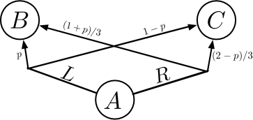
Figure 1: Two-stage distributionally robust MDP with a non-$(\mathrm{s},\mathrm{a})$-rectangular ambiguity set.

Example 2.1.

Consider a two-stage problem with three states $\{s_{A},s_{B},s_{C}\}$. Suppose ${\cal S}_{1}=\{s_{A}\}$, ${\cal S}_{2}=\{s_{B},s_{C}\}$ and there are two actions $a_{L}$ and $a_{R}$ at state $s_{A}$, i.e. ${\cal A}_{1}=\{a_{L},a_{R}\}$. In addition, the cost functions are given by $c_{1}\equiv 0$, and $c_{2}(s_{B})=v_{B}$ and $c_{2}(s_{C})=v_{C}$ for some constants $v_{B}>v_{C}$. In the considered setting, for the corresponding transition kernel $P_{1}$ we only need to specify the probability $P_{1}(s_{B}|s_{A},a_{L})$ of moving to the state $s_{B}$ conditional on action $a_{L}$, and the probability $P_{1}(s_{B}|s_{A},a_{R})$ conditional on action $a_{R}$, since $P_{1}(s_{C}|s_{A},a_{L})=1-P_{1}(s_{B}|s_{A},a_{L})$ and $P_{1}(s_{C}|s_{A},a_{R})=1-P_{1}(s_{B}|s_{A},a_{R})$. Let us consider the ambiguity set at stage $t=1$ defined as

$${\cal P}_{1}:=\big{\{}P_{1}:P_{1}(s_{B}|s_{A},a_{L})=p,\;P_{1}(s_{B}|s_{A},a_{R})=(1+p)/3,\;p\in[0,1]\big{\}}$$ (2.23)

(see Figure 1). The corresponding set ${\mathfrak{P}}^{1}_{s_{1},a_{1}}$, defined in (2.20), is determined by a kernel from the ambiguity set ${\cal P}_{1}$. It follows then by (2.21) that the ambiguity set ${\cal P}_{1}$ is not $(\mathrm{s},\mathrm{a})$-rectangular.

On the other hand, since $c_{1}\equiv 0$ and $V_{2}(s_{B})=c_{2}(s_{B})$ is bigger than $V_{2}(s_{C})=c_{2}(s_{C})$, we have that kernel $P_{1}^{*}$ from the set ${\cal P}_{1}$ for $p=1$, i.e., defined as

$$P_{1}^{*}(s_{B}|s_{A},a_{L})=1,~{}P_{1}^{*}(s_{B}|s_{A},a_{R})=\tfrac{2}{3},$$

satisfies the condition of Assumption 2.1(b). $\hfill\square$

The above example falls into a broader class of ambiguity set defined below.

Definition 2.2 ($\mathrm{r}$-rectangularity, [6, 5]).

The ambiguity set ${\cal P}_{t}$ is said to be $\mathrm{r}$-rectangular if there exist sets $\mathcal{W}_{1}^{t},\ldots,\mathcal{W}_{m}^{t}\subseteq\mathbb{R}^{\left|{\cal S}_{t+1}\right|}$, and for every $s_{t}\in{\cal S}_{t}$ and $a_{t}\in{\cal A}(s_{t})$, one can choose nonnegative numbers $\kappa^{s_{t},a_{t}}_{1},...,\kappa^{s_{t},a_{t}}_{m}$ such that every $P_{t}\in{\cal P}_{t}$ can be represented as probability vector of the form

$$P_{t}(\cdot|s_{t},a_{t})=\textstyle\sum\nolimits_{i=1}^{m}\kappa^{s_{t},a_{t}}_{i}w_{i}$$ (2.24)

for some $w_{i}\in\mathcal{W}_{i}^{t}$, $i=1,...,m$.

Remark 2.3.

The above definition of $\mathrm{r}$-rectangularity is slightly weaker than the one considered in [5, 6]. Indeed, $\mathrm{r}$-rectangularity in [6, 5] requires additionally that $\mathcal{W}_{i}\subseteq\Delta_{|{\cal S}_{t+1}|}$ and that $\textstyle\sum\nolimits_{i=1}^{m}\kappa^{s_{t},a_{t}}_{i}=1$. This additional condition is sufficient for $\textstyle\sum\nolimits_{i=1}^{m}\kappa^{s_{t},a_{t}}_{i}w_{i}$ to be a probability vector, although is not necessary. Indeed, the ambiguity set ${\cal P}_{1}$ of Example 2.1 (defined in equation (2.23)) satisfies $\mathrm{r}$-rectangularity by taking $m=3$ and $\kappa^{A,L}_{1}=1$, $\kappa^{A,L}_{2}=0$, $\kappa^{A,L}_{3}=1$, $\kappa^{A,R}_{1}=0$, $\kappa^{A,R}_{2}=1$, $\kappa^{A,R}_{3}=\tfrac{1}{3}$, $\mathcal{W}_{1}=\{w_{1}\}$, $\mathcal{W}_{2}=\{w_{2}\}$, $\mathcal{W}_{3}=\{w_{3}^{p}:p\in[0,1]\}$, with $w_{1}=(0,1)\in{\mathbb{R}}^{2}$, $w_{2}=(\tfrac{1}{3},\tfrac{2}{3})\in{\mathbb{R}}^{2}$ and $w_{3}^{p}=(p,-p)\in{\mathbb{R}}^{2}$. $\hfill\square$

It can be seen that by taking $m=\left|{\cal S}_{t}\right|\cdot\left|{\cal A}_{t}(s_{t})\right|$, with proper specification of the coefficients $\{\kappa^{s_{t},a_{t}}_{i}\}$ and sets $\{\mathcal{W}^{t}_{i}\}$, every $(\mathrm{s},\mathrm{a})$-rectangular set can be represented as an $\mathrm{r}$-rectangular set. We proceed to verify Assumption 2.1(b) if the costs $c_{t}$ do not depend on the next state $s_{t+1}$.

Proposition 2.4.

Suppose that the costs $c_{t}(s_{t},a_{t})$ do not depend on $s_{t+1}$, and the ambiguity sets ${\cal P}_{t}$, $t=1,...,T$, are $\mathrm{r}$-rectangular. Then Assumption 2.1(b) holds, and the conclusions (i) - (iv) of Theorem 2.1 follow.

Proof.

For $\mathrm{r}$-rectangular sets the maximization problem in (2.17) is equivalent to

$$\max\limits_{P_{t}\in{\cal P}_{t}} \!\!\!\textstyle\sum\nolimits_{s_{t+1}\in{\cal S}_{t+1}}\textstyle\sum\nolimits_{a_{t}\in{\cal A}(s_{t})}P_{t}(s_{t+1}|s_{t},a_{t})\mu_{t}(a_{t})\big{[}c_{t}(s_{t},a_{t})+V_{t+1}(s_{t+1})\big{]}$$

$$=\max_{w_{i}\in\mathcal{W}_{i},1\leq i\leq m}\left\{\textstyle\sum\nolimits_{a_{t}\in{\cal A}(s_{t})}\mu_{t}(a_{t})c_{t}(s_{t},a_{t})+\textstyle\sum\nolimits_{a_{t}\in{\cal A}(s_{t})}\mu_{t}(a_{t})\Big{(}\textstyle\sum\nolimits_{i=1}^{m}\kappa^{s_{t},a_{t}}_{i}\cdot w_{i}^{\top}V_{t+1}\Big{)}\right\},$$

where we denote by $V_{t+1}$ the $|{\cal S}_{t+1}|$-dimensional vector with components $V_{t+1}(s_{t+1})$, $s_{t+1}\in{\cal S}_{t+1}$, and $a^{\top}b=\textstyle\sum\nolimits_{i=1}^{n}a_{i}b_{i}$ is the scalar product of vectors $a,b\in{\mathbb{R}}^{n}$.

Since $\kappa^{s_{t},a_{t}}_{i}\geq 0$, in order to satisfy Assumption 2.1(b) it suffices to choose $P_{t}^{*}$ defined as

$$P_{t}^{*}(\cdot|s_{t},a_{t}):=\textstyle\sum\nolimits_{i=1}^{m}\kappa^{s_{t},a_{t}}_{i}w_{i}^{*},$$ (2.25)

where $w_{i}^{*}\in\mathop{\rm arg\,max}\limits_{w_{i}\in\mathcal{W}^{t}_{i}}w_{i}^{\top}V_{t+1}$. ∎

We now proceed to introduce the second condition that requires the convexity of state-wise marginalization of the ambiguity set ${\cal P}_{t}$. As will be shown shortly, such a condition can be used to certify strong duality in the absence of Assumption 2.1.

Assumption 2.2.

The state-wise marginalization of ${\cal P}_{t}$, defined as

$${\mathfrak{P}}^{t}_{s_{t}}:=\{q_{t}\in\Delta_{|{\cal S}_{t+1}\times{\cal A}_{t}(s_{t})|}:q_{t}(\cdot,\cdot)=P_{t}(\cdot|s_{t},\cdot)~{}\text{for some}~{}P_{t}\in{\cal P}_{t}\},$$ (2.26)

is convex.

It can be noted that the above assumption holds if the set ${\cal P}_{t}$ is convex.

Theorem 2.2.

Suppose Assumption 2.2 is fulfilled. Then the following holds.

• There exists a saddle point $(\pi_{t}^{*},P_{t}^{*})$ for the min-max problem (2.7), and hence there is no duality gap between the primal problem (2.1) and its dual (2.13).

• The primal problem (2.1) has a non-randomized optimal policy iff the min-max problem (2.10) has a saddle point for all $t=1,...,T$, and $s_{t}\in{\cal S}_{t}$.

Proof.

Clearly, (2.7) is equivalent to the following optimization problem

$$\min_{\pi_{t}(\cdot|s_{t})\in\Delta_{|{\cal A}_{t}(s_{t})|}}\sup_{P_{t}(\cdot|s_{t},\cdot)\in{\mathfrak{P}}_{s_{t}}^{t}}\textstyle\sum\nolimits\limits_{s_{t+1}\in{\cal S}_{t+1}}\textstyle\sum\nolimits\limits_{a_{t}\in{\cal A}_{t}(s_{t})}P_{t}(s_{t+1}|s_{t},a_{t})\pi_{t}(a_{t}|s_{t})\big{[}c_{t}(s_{t},a_{t},s_{t+1})+V_{t+1}(s_{t+1})\big{]}.$$ (2.27)

The objective function of problem (2.27) is linear with respect to $\pi_{t}(\cdot|s_{t})$ and linear with respect to $P_{t}(\cdot|s_{t},\cdot)$, and both sets $\Delta_{|{\cal A}_{t}(s_{t})|}$ and ${\mathfrak{P}}_{s_{t}}^{t}$ are convex and the set $\Delta_{|{\cal A}_{t}(s_{t})|}$ is compact. Therefore the strong duality follows by Sion’s theorem. Moreover the primal and dual problems posses optimal solutions and hence there exists the corresponding saddle point. This completes the proof of (i).

Now let us observe that the minimum in the max-min problem (2.12) is always attained at Dirac measure, and hence we can write

$$Q_{t}(s_{t})=\max_{P_{t}\in{\cal P}_{t}}\min_{a_{t}\in{\cal A}_{t}(s_{t})}\textstyle\sum\nolimits\limits_{s_{t+1}\in{\cal S}_{t+1}}P_{t}(s_{t+1}|s_{t},a_{t})\big{[}c_{t}(s_{t},a_{t},s_{t+1})+Q_{t+1}(s_{t+1})\big{]}.$$ (2.28)

Suppose that (2.10) has a saddle point $(a_{t}^{*},P_{t}^{*})\in{\cal A}_{t}(s_{t})\times{\cal P}_{t}$. Then $(a_{t}^{*},P_{t}^{*})$ is a saddle point of (2.28), and hence $\{\delta_{a^{*}_{t}(s_{t})}\}$ is a non-randomized optimal policy of the controller. Conversely suppose that the primal problem has a non-randomized policy. By (i) we have that there is no duality gap between the primal and dual problems. Therefore there is saddle point $(\pi_{t}^{*},P_{t}^{*})$ with $\pi(\cdot|s_{t})$ being Dirac measure. This completes the proof of (ii). ∎

We next introduce an example demonstrating the essential role of convexity in Assumption 2.2.

Example 2.2.

Consider the same MDP as defined in Example 2.1, except that we have

$${\cal P}_{1}=\big{\{}P_{1}:P_{1}(s_{B}|s_{A},a_{L})=p,~{}P_{1}(s_{B}|s_{A},a_{R})=1-p,\;p\in[0,\tfrac{1}{4}]\cup[\tfrac{3}{4},1]\}.$$

Direct computation shows

$$V_{1}(s_{A}) =\min_{\mu\in\Delta_{\{L,R\}}}\max_{P_{1}\in{\cal P}_{1}}\textstyle\sum\nolimits_{s_{2}\in{\cal S}_{2}}\textstyle\sum\nolimits_{a_{1}\in\{a_{L},a_{R}\}}P_{1}(s_{2}|s_{A},a_{1})\mu(a_{1})c_{2}(s_{2})=\tfrac{v_{B}+v_{C}}{2},$$

$$Q_{1}(s_{A}) =\max_{P_{1}\in{\cal P}_{1}}\min_{\mu\in\Delta_{\{L,R\}}}\textstyle\sum\nolimits_{s_{2}\in{\cal S}_{2}}\textstyle\sum\nolimits_{a_{1}\in\{a_{L},a_{R}\}}P_{1}(s_{2}|s_{A},a_{1})\mu(a_{1})c_{2}(s_{2})=\tfrac{1}{4}v_{B}+\tfrac{3}{4}v_{C},$$ (2.29)

and hence $Q_{1}(s_{A})<V_{1}(s_{A})$. $\hfill\square$

As Example 2.2 shows, without the convexity in Assumption 2.2 , the weak duality (2.15) can be strict. On the other hand, with Assumption 2.2, Theorem 2.2 allows us to certify strong duality when Assumption 2.1 does not hold. It should be noted that in this case the optimal policies of the controller can be all randomized. This should be contrasted with conclusion (iii) of Theorem 2.1, which always certifies the existence of non-randomized optimal policies. The next example illustrates this aforementioned observation.

Example 2.3.

Consider the same MDP as defined in Example 2.2, except that in the definition of ${\cal P}_{1}$ we let $p\in[0,1]$. Direct computation shows that when $\mu=\delta_{a_{{}_{L}}}$, the unique solution of (2.17) is given by $P_{1}(s_{B}|s_{A},a_{L})=1$ and $P_{1}(s_{B}|s_{A},a_{R})=0$. In comparison, when $\mu=\delta_{a_{R}}$, the unique solution of (2.17) is given by $P_{1}(s_{B}|s_{A},a_{L})=0$ and $P_{1}(s_{B}|s_{A},a_{R})=1$. Consequently Assumption 2.1(a) does not hold. Nevertheless, ${\cal P}^{1}_{s_{A}}$ is convex and closed, and hence Theorem 2.2 applies and strong duality holds. Finally, it can be readily verified that the optimal policy $\pi^{*}$ of (2.1) is unique and is given by

$$\pi^{*}_{1}(a_{L}|s_{A})=\pi^{*}_{1}(a_{R}|s_{A})=1/2.$$

Note that the policy $\pi^{*}$ is randomized. $\hfill\square$

Remark 2.4 (Nature’s Randomized Policies).

It is also possible to consider randomized policies of the nature when the kernel $P_{t}$ is chosen at random according to a probability distribution supported on the ambiguity set ${\cal P}_{t}$. Then the counterpart of dynamic equations (2.7) can be written as

$$V_{t}(s_{t})=\min_{\pi_{t}(\cdot|s_{t})\in\Delta_{|{\cal A}_{t}(s_{t})|}}\sup_{D_{t}\in{\mathfrak{D}}_{t}}{\mathbb{E}}_{P_{t}\sim D_{t}}{\mathbb{E}}^{\pi_{t},P_{t}}[c_{t}(s_{t},a_{t},s_{t+1})+V_{t+1}(s_{t+1})],$$ (2.30)

where ${\mathfrak{D}}_{t}$ is the set of probability distributions on ${\cal P}_{t}$ equipped with its Borel sigma algebra. By Sion’s theorem the min-max problem (2.30) has a saddle point (note that here the existence of saddle point does not require the convexity of ${\mathfrak{D}}_{t}$). By arguments similar to the proof of part (ii) of Theorem 2.2, we have here that the nature possesses a non-randomized policy iff the min-max problem (2.7) has a saddle point for all $t=1,...,T,$ and $s_{t}\in{\cal S}_{t}$. $\hfill\square$

2.2 History-dependent policies

In this section we discuss history-dependent policies of the controller and/or the nature. We denote by $\widehat{\Pi}$ and $\widehat{\Gamma}$ the sets of history-dependent policies of the controller and the nature, respectively, and consider the counterparts of the primal problem (2.1) and its dual (2.13) when $\Pi$ and $\Gamma$ are replaced by their history-dependent counterparts $\widehat{\Pi}$ and $\widehat{\Gamma}$.

Proposition 2.5.

The following holds. (i) Suppose the controller is Markovian and the nature is history-dependent, i.e., consider the problem

$$\min_{\pi\in\Pi}\max_{\gamma\in\widehat{\Gamma}}{\mathbb{E}}^{\pi,\gamma}\left[\textstyle\sum\nolimits_{t=1}^{T}c_{t}(s_{t},a_{t},s_{t+1})+c_{T+1}(s_{T+1})\right].$$ (2.31)

Then the dynamic equations (2.3) and (2.7) still hold.

(ii) Suppose both the controller and the nature are history-dependent, i.e., consider the problem

$$\min_{\pi\in\widehat{\Pi}}\max_{\gamma\in\widehat{\Gamma}}{\mathbb{E}}^{\pi,\gamma}\left[\textstyle\sum\nolimits_{t=1}^{T}c_{t}(s_{t},a_{t},s_{t+1})+c_{T+1}(s_{T+1})\right].$$ (2.32)

Then for any $\pi\in\widehat{\Pi}$, we have ${\cal V}^{\pi}_{{\mathfrak{h}}_{T}}(s_{T+1})=c(s_{T+1})$, and for $t=T,...,1$,

$${\cal V}^{\pi}_{{\mathfrak{h}}_{t-1}}(s_{t})=\max_{P_{t}\in{\cal P}_{t}}{\textstyle\sum\nolimits_{s_{t+1}\in{\cal S}_{t+1}}\textstyle\sum\nolimits_{a_{t}\in{\cal A}_{t}(s_{t})}P_{t}(s_{t+1}|s_{t},a_{t})\pi_{t}(a_{t}|{\mathfrak{h}}_{t-1},s_{t})\big{[}c_{t}(s_{t},a_{t},s_{t+1})+{\cal V}^{\pi}_{{\mathfrak{h}}_{t}}(s_{t+1})\big{]}},$$ (2.33)

where ${\cal V}^{\pi}_{{\mathfrak{h}}_{t-1}}(s_{t})$ is equal to the optimal value of problem

$$\max_{\gamma\in\widehat{\Gamma}}{\mathbb{E}}^{\pi,\gamma}\left[\textstyle\sum\nolimits_{i=t}^{T}c_{i}(s_{i},a_{i},s_{i+1})+c_{T+1}(s_{T+1})\large|{\mathfrak{h}}_{t-1},s_{t}\right].$$ (2.34)

Moreover, $V_{t}(s_{t})$ defined in (2.7), is equal to the optimal value of

$$\min_{\pi\in\widehat{\Pi}}\max_{\gamma\in\widehat{\Gamma}}{\mathbb{E}}^{\pi,\gamma}\left[\textstyle\sum\nolimits_{i=t}^{T}c_{i}(s_{i},a_{i},s_{i+1})+c_{T+1}(s_{T+1})\big{|}{\mathfrak{h}}_{t-1},s_{t}\right].$$ (2.35)

Proof.

For claim (i), note that the argument of Proposition 2.1 holds even if the nature uses history-dependent policies, since optimizing over Markovian policies is the same as optimizing over history-dependent policies for regular MDPs. Consequently Proposition 2.2 also holds.

We proceed to establish claim (ii). Let us first consider (2.34). Fixing any $\gamma\in\widehat{\Gamma}$, it is immediate that ${\cal V}^{\pi,\gamma}_{{\mathfrak{h}}_{T}}(s_{T+1})=c(s_{T+1})$,

$${\cal V}^{\pi,\gamma}_{{\mathfrak{h}}_{t-1}}(s_{t})={\textstyle\sum\nolimits_{s_{t+1}\in{\cal S}_{t+1}}\textstyle\sum\nolimits_{a_{t}\in{\cal A}_{t}(s_{t})}P_{t}(s_{t+1}|s_{t},a_{t})\pi_{t}(a_{t}|{\mathfrak{h}}_{t-1},s_{t})\big{[}c_{t}(s_{t},a_{t},s_{t+1})+{\cal V}^{\pi,\gamma}_{{\mathfrak{h}}_{t}}(s_{t+1})\big{]}}$$ (2.36)

defines $\{{\cal V}^{\pi,\gamma}_{{\mathfrak{h}}_{t-1}}\}$ such that

$${\cal V}^{\pi,\gamma}_{{\mathfrak{h}}_{t-1}}(s_{t})={\mathbb{E}}^{\pi,\gamma}\left[\textstyle\sum\nolimits_{i=t}^{T}c_{i}(s_{i},a_{i},s_{i+1})+c_{T+1}(s_{T+1})\large|{\mathfrak{h}}_{t-1},s_{t}\right].$$

Here $P_{t}$ in (2.36) is specified by nature’s policy $\gamma$, i.e., $P_{t}=\gamma_{t}({\mathfrak{h}}_{t-1},s_{t})$. We now show by induction that $V^{\pi}_{{\mathfrak{h}}_{t}}\geq{\cal V}^{\pi,\gamma}_{{\mathfrak{h}}_{t}}$ for $t=T,\ldots,0$. The claim is obvious at $t=T$. In addition,

$${\cal V}^{\pi}_{{\mathfrak{h}}_{t-1}}(s_{t}) \overset{(a)}{\geq}\max_{P_{t}^{\prime}\in{\cal P}_{t}}{\textstyle\sum\nolimits_{s_{t+1}\in{\cal S}_{t+1}}\textstyle\sum\nolimits_{a_{t}\in{\cal A}_{t}(s_{t})}P_{t}^{\prime}(s_{t+1}|s_{t},a_{t})\pi_{t}(a_{t}|{\mathfrak{h}}_{t-1},s_{t})\big{[}c_{t}(s_{t},a_{t},s_{t+1})+{\cal V}^{\pi,\gamma}_{{\mathfrak{h}}_{t}}(s_{t+1})\big{]}}$$

$${\geq}{\textstyle\sum\nolimits_{s_{t+1}\in{\cal S}_{t+1}}\textstyle\sum\nolimits_{a_{t}\in{\cal A}_{t}(s_{t})}P_{t}(s_{t+1}|s_{t},a_{t})\pi_{t}(a_{t}|{\mathfrak{h}}_{t-1},s_{t})\big{[}c_{t}(s_{t},a_{t},s_{t+1})+{\cal V}^{\pi,\gamma}_{{\mathfrak{h}}_{t}}(s_{t+1})\big{]}}$$

$$\overset{(b)}{=}{\cal V}^{\pi,\gamma}_{{\mathfrak{h}}_{t-1}}(s_{t}),$$

from which we complete the induction step. Here $(a)$ follows from the induction hypothesis, and $(b)$ follows from (2.36).

Now let $\tilde{\gamma}$ be the history-dependent policy of the nature that attains the maximum in (2.33), then from (2.36) it holds that $V^{\pi}_{{\mathfrak{h}}_{t}}={\cal V}^{\pi,\tilde{\gamma}}_{{\mathfrak{h}}_{t}}$. Consequently, we obtain $V^{\pi}_{{\mathfrak{h}}_{t}}=\max_{\gamma}{\cal V}^{\pi,\gamma}_{{\mathfrak{h}}_{t}}$ and (2.34).

With (2.33) in place, one can follow essentially the same lines as in the proof of Proposition 2.2 and readily obtain that dynamic equations $V_{{\mathfrak{h}}_{T}}(s_{T+1})=c_{T+1}(s_{T+1})$,

$$V_{{\mathfrak{h}}_{t-1}}(s_{t})=\min_{\pi_{t}(\cdot|{\mathfrak{h}}_{t-1},s_{t})\in\Delta_{|{\cal A}_{t}(s_{t})|}}\max_{P_{t}\in{\cal P}_{t}}\textstyle\sum\nolimits\limits_{s_{t+1}\in{\cal S}_{t+1}}\textstyle\sum\nolimits\limits_{a_{t}\in{\cal A}_{t}(s_{t})}P_{t}(s_{t+1}|s_{t},a_{t})\pi_{t}(a_{t}|{\mathfrak{h}}_{t-1},s_{t})\big{[}c_{t}(s_{t},a_{t},s_{t+1})+V_{{\mathfrak{h}}_{t}}(s_{t+1})\big{]},$$ (2.37)

define $V_{{\mathfrak{h}}_{t-1}}(s_{t})$, which equals the optimal value of (2.35). To conclude our proof for claim (ii), it suffices to show that $V_{{\mathfrak{h}}_{t}}(\cdot)$ only depends on $t+1$ and does not depend on ${\mathfrak{h}}_{t}$. We now show this by induction. Clearly, this holds trivially at $t=T$. Suppose the claim holds at stage $t$, then from (2.37) we obtain

$$V_{{\mathfrak{h}}_{t-1}}(s_{t})=\min_{q_{t}\in\Delta_{|{\cal A}_{t}(s_{t})|}}\max_{P_{t}\in{\cal P}_{t}}\textstyle\sum\nolimits\limits_{s_{t+1}\in{\cal S}_{t+1}}\textstyle\sum\nolimits\limits_{a_{t}\in{\cal A}_{t}(s_{t})}P_{t}(s_{t+1}|s_{t},a_{t})q_{t}(a_{t})\big{[}c_{t}(s_{t},a_{t},s_{t+1})+V_{t+1}(s_{t+1})\big{]},$$

from which it is clear that $V_{{\mathfrak{h}}_{t-1}}(\cdot)$ only depends on $t$ but not ${\mathfrak{h}}_{t-1}$. From this we complete the induction step and the proof for claim (ii) is completed. ∎

In [16, section 5] are presented examples when the controller is allowed history-dependent policies while the nature is Markovian, which are not amendable to writing dynamic programming equations similar to (2.7). We show now that the respective dynamic equations still hold provided there is no duality gap between the primal problem (2.1) and its dual (2.13).

Proposition 2.6.

Consider counterpart of (2.1) when the controller uses history-dependent policies $\widehat{\Pi}$ and the nature uses Markovian policies $\Gamma$, i.e.,

$$\min_{\pi\in\widehat{\Pi}}\max_{\gamma\in{\Gamma}}{\mathbb{E}}^{\pi,\gamma}\left[\textstyle\sum\nolimits_{t=1}^{T}c_{t}(s_{t},a_{t},s_{t+1})+c_{T+1}(s_{T+1})\right].$$ (2.38)

If $\mathrm{OPT}(\ref{mdp-1})=\mathrm{OPT}(\ref{dual-1})$ holds, then there exists an optimal policy of (2.38) that is Markovian, and dynamic equations (2.7) still hold for problem (2.38).

Proof.

Let us denote $f(\pi,\gamma):={\mathbb{E}}^{\pi,\gamma}[\textstyle\sum\nolimits_{t=1}^{T}c_{t}(s_{t},a_{t},s_{t+1})+c_{T+1}(s_{T+1})]$. Then the following is immediate:

$$\max_{\gamma\in\Gamma}\min_{\pi\in\Pi}f(\pi,\gamma)\overset{(a)}{=}\max_{\gamma\in\Gamma}\min_{\pi\in\widehat{\Pi}}f(\pi,\gamma)\leq\min_{\pi\in\widehat{\Pi}}\max_{\gamma\in\Gamma}f(\pi,\gamma)\leq\min_{\pi\in{\Pi}}\max_{\gamma\in\Gamma}f(\pi,\gamma),$$

where $(a)$ follows from the fact that $\min_{\pi\in\widehat{\Pi}}f(\pi,\gamma)$ is a regular MDP of the controller as the nature is Markovian, subsequently for the controller minimizing over Markovian policies is equivalent to minimizing over history-dependent policies. If $\mathrm{OPT}(\ref{mdp-1})=\mathrm{OPT}(\ref{dual-1})$ holds, then clearly all the above inequalities indeed hold with equality, from which we conclude the proof. ∎

3 Static formulation of distributionally robust MDP

Let us consider the following static formulation of distributionally robust MDP,

$$\min_{\pi\in\Pi}\sup_{P_{1}\in{\cal P}_{1},\ldots,P_{T}\in{\cal P}_{T}}{\mathbb{E}}^{\pi,\{P_{t}\}_{t=1}^{T}}\left[\textstyle\sum\nolimits_{t=1}^{T}c_{t}(s_{t},a_{t},s_{t+1})+c_{T+1}(s_{T+1})\right].$$ (3.1)

As it was also mentioned in Remark 2.2, in some publications the static formulation is referred to as robust MDPs. The essential difference between (3.1) and the game formulation (2.1) is that in (3.1) the nature chooses the kernels prior to the realization of the Markov process. The dual of (3.1) is

$$\sup_{P_{1}\in{\cal P}_{1},\ldots,P_{T}\in{\cal P}_{T}}\min_{\pi\in\Pi}{\mathbb{E}}^{\pi,\{P_{t}\}_{t=1}^{T}}\left[\textstyle\sum\nolimits_{t=1}^{T}c_{t}(s_{t},a_{t},s_{t+1})+c_{T+1}(s_{T+1})\right].$$ (3.2)

Formulations (3.1) and (3.2) can be viewed as the static counterparts of the respective problems (2.1) and (2.13).

Below we first discuss when the static formulation (for both primal and dual problems) is equivalent to the game formulation discussed in Section 2.1.

Theorem 3.1.

The following holds. (i) If for any policy $\pi\in\Pi$, there exists a solution $P_{t}^{*}$ of (2.3) that is independent of $s_{t}$, for every $s_{t}\in{\cal S}_{t}$ and $t=1,\ldots,T$, then the primal problem (2.1) of the game and its static counterpart (3.1) are equivalent, i.e.,

$$\mathrm{OPT}\eqref{mdp-1}=\mathrm{OPT}\eqref{eq_static_formulation},$$ (3.3)

and the dynamic equations (2.7) hold for the static problem (3.1) as well.

(ii) If for problem (2.12) (not necessarily having a saddle point), there exits a solution $P_{t}^{*}$ such that $P_{t}^{*}$ is independent of $s_{t}$, for every $s_{t}\in{\cal S}_{t}$ and $t=1,\ldots,T$, then the dual problem (2.13) of the game and its static counterpart (3.2) are equivalent, i.e.,

$$\mathrm{OPT}\eqref{dual-1}=\mathrm{OPT}\eqref{eq_static_formulation_dual},$$ (3.4)

and the dynamic equations (2.12) hold for the static problem (3.2) as well.

Proof.

For the claim (i), given the specified condition, it can be readily seen that for any $\pi\in\Pi$,

$$\begin{array}[]{lll}\max\limits_{\gamma\in\Gamma}&{\mathbb{E}}^{\pi,\gamma}\left[\textstyle\sum\nolimits_{t=1}^{T}c_{t}(s_{t},a_{t},s_{t+1})+c_{T+1}(s_{T+1})\right]\\ &={\mathbb{E}}^{\pi,\{P_{t}^{*}\}_{t=1}^{T}}\left[\textstyle\sum\nolimits_{t=1}^{T}c_{t}(s_{t},a_{t},s_{t+1})+c_{T+1}(s_{T+1})\right]\\ &\leq\sup\limits_{P_{1}\in{\cal P}_{1},\ldots,P_{T}\in{\cal P}_{T}}{\mathbb{E}}^{\pi,\{P_{t}\}_{t=1}^{T}}\left[\textstyle\sum\nolimits_{t=1}^{T}c_{t}(s_{t},a_{t},s_{t+1})+c_{T+1}(s_{T+1})\right].\end{array}$$ (3.5)

On the other hand, it holds trivially that the first term in (3.5) is at least that of the last term in the above relation, which implies that the above inequality holds with equality. Since this holds for any $\pi\in\Pi$, the claim (i) follows.

For the claim (ii), from the specified condition we have that for the dual problem (2.13), the optimal policy is given by $\gamma_{t}^{*}(s_{t})=P_{t}^{*}$, and consequently

$$\mathrm{OPT}\eqref{dual-1} =\min_{\pi\in\Pi}{\mathbb{E}}^{\pi,\gamma^{*}}\left[\textstyle\sum\nolimits_{t=1}^{T}r_{t}(s_{t},a_{t},s_{t+1})+r_{T+1}(s_{T+1})\right]$$

$$=\min_{\pi\in\Pi}{\mathbb{E}}^{\pi,\{P_{t}^{*}\}_{t=1}^{T}}\left[\textstyle\sum\nolimits_{t=1}^{T}c_{t}(s_{t},a_{t},s_{t+1})+c_{T+1}(s_{T+1})\right]\leq\mathrm{OPT}\eqref{eq_static_formulation_dual}.$$

Combining the above relation with $\mathrm{OPT}\eqref{eq_static_formulation_dual}\leq\mathrm{OPT}\eqref{dual-1}$ yields the claim (ii). ∎

Clearly, the conditions in Theorem 3.1 hold for $(\mathrm{s},\mathrm{a})$- and $\mathrm{r}$-rectangular sets discussed in Section 2.1. Below we introduce another class of commonly used ambiguity sets for the static formulation that trivially satisfies these conditions (the verification uses a similar argument as in Proposition 2.3).

Definition 3.1 ($\mathrm{s}$-rectangularity, [15, 17]).

The ambiguity set ${\cal P}_{t}$ is said to be $\mathrm{s}$-rectangular if the following holds:

$${\cal P}_{t}=\{P_{t}:P_{t}(\cdot|s_{t},\cdot)\in{\mathfrak{P}}^{t}_{s_{t}},~{}\forall s_{t}\in{\cal S}_{t}\},$$

where ${\mathfrak{P}}^{t}_{s_{t}}$ is defined as in (2.26).

Theorem 3.1 allows one to immediately obtain the dynamic equations of the static formulation for the ambiguity sets commonly used for the static formulation.

Corollary 3.1.

For the $(\mathrm{s},\mathrm{a})$-, $\mathrm{s}$- and $\mathrm{r}$-rectangular sets, the game formulation is equivalent to the static formulation. In particular, (2.7) provides the dynamic equations of the primal problem (3.1) of the static formulation, and (2.12) provides the dynamic equations of the dual problem (3.2) of the static formulation.

Remark 3.1.

At this point it might be worth mentioning that prior studies of the static formulation for each of the ambiguity sets adopt a case-by-case analysis in establishing the corresponding dynamic equations (cf., [17, 6, 7, 9]). The formulation equivalence we consider and establish here has not been discussed in the prior literature. In particular, this formulation equivalence allows one to provide a unified treatment for different ambiguity sets with rather simple arguments. $\hfill\square$

As the last result in this section, we are ready to discuss the duality of the static formulation.

Theorem 3.2.

Suppose for every $t=1,\ldots T$ and $s_{t}\in{\cal S}_{t}$, a saddle point $(\pi_{t}^{*},P_{t}^{*})$ exists for (2.7), and $P_{t}^{*}$ does not depend on $s_{t}$, then

$$\mathrm{OPT}\eqref{mdp-1}=\mathrm{OPT}\eqref{dual-1}=\mathrm{OPT}\eqref{eq_static_formulation}=\mathrm{OPT}\eqref{eq_static_formulation_dual}.$$ (3.6)

That is, the static formulation (for both primal and dual problems) is equivalent to the game formulation, and the strong duality holds for the static formulation.

Proof.

From Remark 2.1, we have $\mathrm{OPT}\eqref{mdp-1}=\mathrm{OPT}\eqref{dual-1}$. Consequently a saddle point of (2.7) is also a saddle point of (2.12). Since $P_{t}^{*}$ does not depend on $s_{t}$, we can invoke the second claim of Theorem 3.1 and obtain that $\mathrm{OPT}\eqref{dual-1}=\mathrm{OPT}\eqref{eq_static_formulation_dual}$. The desired claim then follows from the additional trivial observations: $\mathrm{OPT}\eqref{eq_static_formulation_dual}\leq\mathrm{OPT}\eqref{eq_static_formulation}\leq\mathrm{OPT}\eqref{mdp-1}$ ∎

Corollary 3.2.

(i) Under Assumption 2.1(b), the conclusions of Theorem 3.2 hold. In particular, for both $(\mathrm{s},\mathrm{a})$- and $\mathrm{r}$-rectangular sets, (3.6) holds. (ii) For $\mathrm{s}$-rectangular sets, if ${\mathfrak{P}}_{s_{t}}^{t}$ is convex (Assumption 2.2) for all $s_{t}\in{\cal S}_{t}$ and $t=1,\ldots,T$, then (3.6) holds.

Proof.

In view of Theorem 3.2 it suffices to verify that a saddle point $(\pi_{t}^{*},P_{t}^{*})$ exists for (2.7) and $P_{t}^{*}$ does not depend on $s_{t}$. This trivially holds for ambiguity sets satisfying Assumption 2.1(b), and in particular, for $(\mathrm{s},\mathrm{a})$- and $\mathrm{r}$-rectangular sets. On the other hand, for $\mathrm{s}$-rectangular sets satisfying Assumption 2.2, the existence of saddle point $(\pi_{t}^{*},P_{t}^{*})$ for (2.7) follows from Theorem 2.2. The fact that $P_{t}^{*}$ can be chosen independent of $s_{t}$ follows trivially using the similar argument in Proposition 2.3 and the definition of $\mathrm{s}$-rectangularity. ∎

Remark 3.2.

Similar to Remark 3.1, the strong duality of the static formulation involving $(\mathrm{s},\mathrm{a})$- and $\mathrm{r}$-rectangular sets has been discussed in [9] and [6] respectively, following a case-by-case analysis. Here our argument differs by first discussing the strong duality of the game formulation and then using the equivalence of the game and static formulations. Both steps are conceptually simple and provides a unifying treatment of different ambiguity sets. In particular, the strong duality discussion of s-rectangular sets for the static formulation seems to be new. $\hfill\square$

It is worth noting here that for $\mathrm{s}$-rectangular sets, the strong duality of the static formulation hinges upon the convexity of $\{{\mathfrak{P}}_{s_{t}}^{t}\}$. Indeed, it can be readily verified that Example 2.2 considers an $\mathrm{s}$-rectangular ambiguity set with non-convex ${\mathfrak{P}}_{s_{A}}^{1}$. Consequently we have

$$\mathrm{OPT}\eqref{mdp-1}=\mathrm{OPT}\eqref{eq_static_formulation}<\mathrm{OPT}\eqref{dual-1}=\mathrm{OPT}\eqref{eq_static_formulation_dual},$$

where the equalities follows from Corollary 3.1, and the strict inequality follows from Example 2.2. The essential role of convexity in the strong duality of static formulations involving $\mathrm{s}$-rectangular sets has not been discussed in [17].

4 Cost-robust MDP

Our discussion so far has focused on ambiguity of the transition kernels. In this section, we show that by following the same lines of argument, one can naturally consider ambiguity on the cost functions. Specifically, we assume in this section that the transition kernels $\{P_{t}\}$ are given (fixed), and there exists a set ${\cal C}_{t}$, $t=1,\ldots,T$, of cost functions. For simplicity we assume that there is no cost ambiguity at $t=T+1$. It is worth noting that since each $c_{t}\in{\cal C}_{t}$ is of the same dimension as the $P_{t}$, we can define $(\mathrm{s,a})$-, $\mathrm{s}$- and $\mathrm{r}$-rectangularity for ${\cal C}_{t}$ in exactly the same manner as in Sections 2 and 3.

4.1 Game formulation of cost-robust MDP

We define the game formulation of cost-robust MDP similarly as in Section 2. In this case, a (Markovian) policy of the nature maps from ${\cal S}_{t}$ into ${\cal C}_{t}$. As before we denote by $\Pi$ and $\Gamma$ the sets of Markovian policies of the controller and the nature, respectively. The corresponding primal problem of the game formulation is

$$\min_{\pi\in\Pi}\max_{\gamma\in\Gamma}{\mathbb{E}}^{\pi,\gamma}\left[\textstyle\sum\nolimits_{t=1}^{T}c_{t}(s_{t},a_{t},s_{t+1})+c_{T+1}(s_{T+1})\right].$$ (4.1)

Given a policy $\{\pi_{t}\}$ of the controller, the nature chooses a policy so as to maximize the total expected cost, i.e.,

$$\max_{\gamma\in\Gamma}{\mathbb{E}}^{\pi,\gamma}\left[\textstyle\sum\nolimits_{t=1}^{T}c_{t}(s_{t},a_{t},s_{t+1})+c_{T+1}(s_{T+1})\right].$$ (4.2)

The following propositions follow the same argument as that of Proposition 2.1 and 2.2.

Proposition 4.1.

Given a policy $\pi\in\Pi$ of the controller, problem (4.2) admits the following dynamic programming equations: ${\cal V}^{\pi}_{T+1}(s_{T+1})=c_{T+1}(s_{T+1})$ and for $t=T,...,1$,

$${\cal V}^{\pi}_{t}(s_{t}) =\max_{c_{t}\in{\cal C}_{t}}\textstyle\sum\nolimits_{s_{t+1}\in{\cal S}_{t+1}}\textstyle\sum\nolimits_{a_{t}\in{\cal A}_{t}(s_{t})}P_{t}(s_{t+1}|s_{t},a_{t})\pi_{t}(a_{t}|s_{t})\big{[}c_{t}(s_{t},a_{t},s_{t+1})+{\cal V}^{\pi}_{t+1}(s_{t+1})\big{]},$$ (4.3)

where ${\cal V}^{\pi}_{t}(s_{t})$ corresponds to the optimal value of problem

$$\max_{\gamma\in\Gamma}{\mathbb{E}}^{\pi,\gamma}\left[\textstyle\sum\nolimits_{i=t}^{T}c_{i}(s_{i},a_{i},s_{i+1})+c_{T+1}(s_{T+1})\right].$$

Furthermore, it holds that

$${\cal V}^{\pi}_{t}(s_{t}) =h_{s_{t}}(\pi_{t}(\cdot|s_{t}))+\textstyle\sum\nolimits_{s_{t+1}\in{\cal S}_{t+1}}\textstyle\sum\nolimits_{a_{t}\in{\cal A}_{t}(s_{t})}P_{t}(s_{t+1}|s_{t},a_{t})\pi_{t}(a_{t}|s_{t}){\cal V}^{\pi}_{t+1}(s_{t+1}),$$ (4.4)

where

$$h_{s_{t}}(x_{t}):=\sup_{{c}_{t}\in{{\cal C}}_{t}}\textstyle\sum\nolimits\limits_{a_{t}\in{\cal A}_{t}(s_{t})}x_{t}(a_{t})\textstyle\sum\nolimits\limits_{s_{t+1}\in{\cal S}_{t+1}}P_{t}(s_{t+1}|s_{t},a_{t})c_{t}(s_{t},a_{t},s_{t+1}).$$ (4.5)

It can be noted that function $h_{s_{t}}(\cdot)$, defined in (4.5), is given by the maximum of linear in $x_{t}\in{\mathbb{R}}^{|{\cal A}_{t}(s_{t})|}$ functions, and hence is convex and positively homogeneous for any $s_{t}\in{\cal S}_{t}$.

Proposition 4.2.

The dynamic programming equations for the primal problem (4.1) are: $V_{T+1}(s_{T+1})=c_{T+1}(s_{T+1})$ and for $t=T,...,1$,

$$V_{t}(s_{t})=\min_{\pi_{t}(\cdot|s_{t})\in\Delta_{|{\cal A}_{t}(s_{t})|}}\max_{c_{t}\in{\cal C}_{t}}\textstyle\sum\nolimits\limits_{s_{t+1}\in{\cal S}_{t+1}}\textstyle\sum\nolimits\limits_{a_{t}\in{\cal A}_{t}(s_{t})}P_{t}(s_{t+1}|s_{t},a_{t})\pi_{t}(a_{t}|s_{t})\big{[}c_{t}(s_{t},a_{t},s_{t+1})+V_{t+1}(s_{t+1})\big{]},$$ (4.6)

where $V_{t}(s_{t})$ corresponds to the optimal value of

$$\min_{\pi\in\Pi}\max_{\gamma\in\Gamma}{\mathbb{E}}^{\pi,\gamma}\left[\textstyle\sum\nolimits_{l=t}^{T}c_{l}(s_{l},a_{l},s_{l+1})+c_{T+1}(s_{T+1})\right].$$

Furthermore, it holds that

$$V_{t}(s_{t}) =\min_{\pi_{t}(\cdot|s_{t})\in\Delta_{|{\cal A}_{t}(s_{t})|}}\left\{h_{s_{t}}(\pi_{t}(\cdot|s_{t}))+\textstyle\sum\nolimits_{s_{t+1}\in{\cal S}_{t+1}}\textstyle\sum\nolimits_{a_{t}\in{\cal A}_{t}(s_{t})}P_{t}(s_{t+1}|s_{t},a_{t})\pi_{t}(a_{t}|s_{t})V_{t+1}(s_{t+1})\right\}.$$ (4.7)

It follows from (4.7) in Proposition 4.2 that the game formulation of cost-robust MDP can be reduced to a regular (i.e., non-robust) MDP with convex policy-dependent cost functions, provided the function $h_{s_{t}}(\cdot)$ is real valued for every $s_{t}\in{\cal S}_{t}$.

Theorem 4.1.

The game formulation (4.1) of cost-robust MDP is equivalent to a regular (i.e., non-robust) MDP with the same state and action spaces and transition kernels. For a given policy $\pi\in\Pi$, the cost of the regular MDP at state $s_{t}\in{\cal S}_{t}$ is given by $h_{s_{t}}(\pi_{t}(\cdot|s_{t}))$.

The dual of problem (4.1) is defined as

$$\max_{\gamma\in\Gamma}\min_{\pi\in\Pi}{\mathbb{E}}^{\pi,\gamma}\left[\textstyle\sum\nolimits_{t=1}^{T}c_{t}(s_{t},a_{t},s_{t+1})+c_{T+1}(s_{T+1})\right].$$ (4.8)

The dynamic programming equations for the dual problem are: $Q_{T+1}(s_{T+1})=c_{T+1}(s_{T+1})$ and for $t=T,...,1$,

$$Q_{t}(s_{t})=\max_{c_{t}\in{\cal C}_{t}}\min_{\pi_{t}(\cdot|s_{t})\in\Delta_{|{\cal A}_{t}(s_{t})|}}\textstyle\sum\nolimits\limits_{s_{t+1}\in{\cal S}_{t+1}}\textstyle\sum\nolimits\limits_{a_{t}\in{\cal A}_{t}(s_{t})}P_{t}(s_{t+1}|s_{t},a_{t})\pi_{t}(a_{t}|s_{t})\big{[}c_{t}(s_{t},a_{t},s_{t+1})+Q_{t+1}(s_{t+1})\big{]}.$$ (4.9)

Similar to Section 2, we now introduce sufficient conditions that certify the strong duality of the game formulation for cost-robust MDP.

Assumption 4.1.

1. For every $s_{t}\in{\cal S}_{t}$ there is a cost function $c^{*}_{t}\in{\cal C}_{t}$, potentially depending on $s_{t}$, with

   $$c^{*}_{t}\in\mathop{\rm arg\,max}\limits_{c_{t}\in{\cal C}_{t}}\textstyle\sum\nolimits_{s_{t+1}\in{\cal S}_{t+1}}\textstyle\sum\nolimits_{a_{t}\in{\cal A}(s_{t})}P_{t}(s_{t+1}|s_{t},a_{t})\mu_{t}(a_{t})\big{[}c_{t}(s_{t},a_{t},s_{t+1})+V_{t+1}(s_{t+1})\big{]},$$ (4.10)

   for any $\mu_{t}\in\Delta_{|A_{t}(s_{t})|}$.

2. There is a cost function $c^{*}_{t}\in{\cal C}_{t}$ such that condition (4.10) holds for all $s_{t}\in{\cal S}_{t}$ and any $\mu_{t}\in\Delta_{|A_{t}(s_{t})|}$.

Suppose that Assumption 4.1(a) holds and consider

$$\pi_{t}^{*}(\cdot|s_{t})=\delta_{a_{t}^{*}(s_{t})}\;\text{ with}\;a_{t}^{*}(s_{t})\in\mathop{\rm arg\,min}_{a_{t}\in{\cal A}_{t}(s_{t})}\textstyle\sum\nolimits\limits_{s_{t+1}\in{\cal S}_{t+1}}P_{t}(s_{t+1}|s_{t},a_{t})\big{[}c^{*}_{t}(s_{t},a_{t},s_{t+1})+V_{t+1}(s_{t+1})\big{]}.$$ (4.11)

It follows directly from (4.10) and (4.11) that $(\pi_{t}^{*},c_{t}^{*})$ is a saddle point of the min-max problem (4.6). Consequently we have the following result.

Theorem 4.2.

Suppose that Assumption 4.1(a) is fulfilled for all $t=1,...,T$, and let $\pi_{t}^{*}(\cdot|s_{t})$ be the minimizer defined in (4.11). Then the following holds:

• $(\pi_{t}^{*},c_{t}^{*})$ is a saddle point of the min-max problem (4.6).

• There is no duality gap between the primal problem (4.1) and its dual (4.8).

• $\{\pi^{*}_{t}\}$ is an optimal (non-randomized) policy of the controller in the primal problem (4.1) and $\gamma_{t}^{*}(s_{t})=c_{t}^{*}$, $t=1,\ldots,T,$ is an optimal policy of the nature considered in the dual problem (4.8) (here $c_{t}^{*}$, viewed as an element of ${\cal C}_{t}$, can depend on $s_{t}\in{\cal S}_{t}$).

• If moreover Assumption 4.1(b) holds, then the above claims hold with $c_{t}^{*}$ independent of $s_{t}$.

An immediate application of Theorem 4.2 yields the following propositions.

Proposition 4.3.

Suppose that the ambiguity sets ${\cal C}_{t}$, $t=1,...,T$, are $(\mathrm{s},\mathrm{a})$-rectangular. Then Assumption 4.1(b) holds, and conclusions (i) - (iv) of Theorem 4.2 follow.

Proposition 4.4.

Suppose the ambiguity sets ${\cal C}_{t}$, $t=1,...,T$, are $\mathrm{r}$-rectangular. Then Assumption 4.1(b) holds, and the conclusions (i) - (iv) of Theorem 4.2 follow.

The following condition can be viewed as the counterpart of Assumption 2.2 for the cost functions.

Assumption 4.2.

The state-wise marginalization of ${\cal C}_{t}$, defined as

$${\mathfrak{C}}^{t}_{s_{t}}:=\{q_{t}:q_{t}(\cdot,\cdot)=c_{t}(\cdot|s_{t},\cdot)~{}\text{for some}~{}c_{t}\in{\cal C}_{t}\},$$ (4.12)

is convex.

Clearly, Assumption 4.2 holds if the set ${\cal C}_{t}$ is convex. The next result then follows from the same argument as in Theorem 2.2.

Theorem 4.3.

Suppose Assumption 4.2 holds. Then

• There exists a saddle point $(\pi_{t}^{*},c_{t}^{*})$ for the min-max problem (4.6).

• There is no duality gap between the primal problem (4.1) and its dual (4.8).

Furthermore, the primal problem (4.1) has a non-randomized optimal policy iff the min-max problem

$$\min_{a_{t}\in{\cal A}_{t}(s_{t})}\max_{c_{t}\in{\cal C}_{t}}\textstyle\sum\nolimits\limits_{s_{t+1}\in{\cal S}_{t+1}}P_{t}(s_{t+1}|s_{t},a_{t})\big{[}c_{t}(s_{t},a_{t},s_{t+1})+V_{t+1}(s_{t+1})\big{]}.$$

has a saddle point for all $t=1,...,T$ and $s_{t}\in{\cal S}_{t}$.

4.2 Static formulation of cost-robust MDP

Let us consider the following static formulation of cost-robust MDP,

$$\min_{\pi\in\Pi}\sup_{c_{1}\in{\cal C}_{1},\ldots,c_{T}\in{\cal C}_{T}}{\mathbb{E}}^{\pi,\{P_{t}\}_{t=1}^{T}}\left[\textstyle\sum\nolimits_{t=1}^{T}c_{t}(s_{t},a_{t},s_{t+1})+c_{T+1}(s_{T+1})\right].$$ (4.13)

The corresponding dual problem is given by

$$\max_{c_{1}\in{\cal C}_{1},\ldots,c_{T}\in{\cal C}_{T}}\inf_{\pi\in\Pi}{\mathbb{E}}^{\pi,\{P_{t}\}_{t=1}^{T}}\left[\textstyle\sum\nolimits_{t=1}^{T}c_{t}(s_{t},a_{t},s_{t+1})+c_{T+1}(s_{T+1})\right].$$ (4.14)

Formulations (4.13) and (4.14) can be viewed as the static counterparts of the respective problems (4.1) and (4.8).

With the same argument as in Theorem 3.1, one can establish the following equivalence of game and static formulations for cost-robust MDP.

Theorem 4.4.

The following holds. (i) If for any policy $\pi\in\Pi$, there exists a solution $c_{t}^{*}$ of (4.3) that is independent of $s_{t}$, for every $s_{t}\in{\cal S}_{t}$ and $t=1,\ldots,T$, then the primal problem (4.1) of the game and its static counterpart (4.13) are equivalent, i.e.,

$$\mathrm{OPT}\eqref{mdp-1_cost}=\mathrm{OPT}\eqref{eq_static_formulation_cost},$$ (4.15)

and the dynamic equations (4.6) hold for the static problem (4.13) as well.

(ii) If for problem (4.9) (not necessarily having a saddle point), there exits a solution $c_{t}^{*}$ such that $c_{t}^{*}$ is independent of $s_{t}$, for every $s_{t}\in{\cal S}_{t}$ and $t=1,\ldots,T$, then the dual problem (4.8) of the game and its static counterpart (4.14) are equivalent, i.e.,

$$\mathrm{OPT}\eqref{dual-1_cost}=\mathrm{OPT}\eqref{eq_static_formulation_dual_cost},$$ (4.16)

and the dynamic equations (4.9) hold for the static problem (4.14) as well.

Corollary 4.1.

For the $(\mathrm{s},\mathrm{a})$-, $\mathrm{s}$- and $\mathrm{r}$-rectangular sets, the game formulation is equivalent to the static formulation for cost-robust MDP. In particular, (4.6) provides the dynamic equations of the primal problem (4.13) of the static formulation, and (4.9) provides the dynamic equations of the dual problem (4.14) of the static formulation.

We now conclude this section by discussing the duality of the static formulation. As before, the following result follows from the same lines as that of Section 2 (i.e., Theorem 3.2).

Theorem 4.5.

Suppose for every $t=1,\ldots T$ and $s_{t}\in{\cal S}_{t}$, a saddle point $(\pi_{t}^{*},c_{t}^{*})$ exists for (4.6), and $c_{t}^{*}$ does not depend on $s_{t}$, then

$$\mathrm{OPT}\eqref{mdp-1_cost}=\mathrm{OPT}\eqref{dual-1_cost}=\mathrm{OPT}\eqref{eq_static_formulation_cost}=\mathrm{OPT}\eqref{eq_static_formulation_dual_cost}.$$ (4.17)

That is, the static formulation (for both primal and dual problems) is equivalent to the game formulation, and the strong duality holds for the static formulation.

Corollary 4.2.

(i) Under Assumption 4.1(b), the conclusions of Theorem 4.5 hold. In particular, for both $(\mathrm{s},\mathrm{a})$- and $\mathrm{r}$-rectangular sets, (4.17) holds. (ii) For $\mathrm{s}$-rectangular sets, if ${\mathfrak{C}}_{s_{t}}^{t}$ is convex (Assumption 4.2) for all $s_{t}\in{\cal S}_{t}$ and $t=1,\ldots,T$, then (4.17) holds.

5 Risk averse setting

In this section we discuss a risk averse formulation of MDPs and its relation to the distributionally robust approach. Consider a finite set $\Omega=\{\omega_{1},...,\omega_{n}\}$ equipped with sigma algebra ${\cal F}$ of all subsets of $\Omega$. Let ${\cal Z}$ be the space of functions $Z:\Omega\to{\mathbb{R}}$. Note that $Z$ can be identified with $n$-dimensional vector with components $Z_{i}=Z(\omega_{i})$, $i=1,...,n$, and hence ${\cal Z}$ can be identified with ${\mathbb{R}}^{n}$. Let ${\cal R}:{\cal Z}\to{\mathbb{R}}$ be a convex functional. Suppose that ${\cal R}$ is monotone, i.e. if $Z\leq Z^{\prime}$, then ${\cal R}(Z)\leq{\cal R}(Z^{\prime})$; positively homogeneous, i.e. ${\cal R}(\lambda Z)=\lambda{\cal R}(Z)$ for any $\lambda\geq 0$ and $Z\in{\cal Z}$; and such that ${\cal R}(Z+a)={\cal R}(Z)+a$ for any $a\in{\mathbb{R}}$ and $Z\in{\cal Z}$. The functional ${\cal R}$ can be viewed as a coherent risk measure defined on the space ${\cal Z}$ of (measurable) functions (cf., [1]). We can refer to [4, 12] for a thorough discussion of coherent risk measures defined on general probability spaces.

It is said that ${\cal R}={\cal R}_{P}$ is law invariant with respect to a probability measure $P$, defined on $(\Omega,{\cal F})$, if ${\cal R}_{P}(Z)$ can be considered as a function of the cumulative distribution function $F_{Z}(z)=P(Z\leq z)$ (e.g., [12, Section 6.3.3]). Law invariant coherent risk measure ${\cal R}_{P}:{\cal Z}\to{\mathbb{R}}$ has the following dual representation, in the distributionally robust form,

$${\cal R}_{P}(Z)=\sup_{q\in{\mathfrak{M}}_{P}}\textstyle\sum\nolimits_{i=1}^{n}q_{i}Z_{i},$$ (5.1)

where ${\mathfrak{M}}_{P}\subset\Delta_{n}$ is a set of probability measures (probability vectors), depending on $P$, such that every $Q\in{\mathfrak{M}}_{P}$ is absolutely continuous with respect to $P$. Note that in the considered setting of finite $\Omega$, measure $Q$ is absolutely continuous with respect to $P$ iff $p_{i}=0$ implies that $q_{i}=0$. Of course if all probabilities $p_{i}$ are positive, any probability measure $Q$ is absolutely continuous with respect to $P$.

Let ${\mathbb{P}}_{t}$ be a specified (reference) transition kernel. Considering ${\mathbb{P}}_{t}(\cdot|s_{t},a_{t})$ as a probability measure on ${\cal S}_{t+1}$, we can consider the corresponding law invariant coherent risk measure ${\cal R}_{{\mathbb{P}}_{t}(\cdot|s_{t},a_{t})}$ depending on $s_{t}\in{\cal S}_{t}$ and $a_{t}\in{\cal A}_{t}(s_{t})$. This suggests the following counterpart of dynamic equations (2.7):

$$V_{t}(s_{t})=\min_{\pi_{t}(\cdot|s_{t})\in\Delta_{|{\cal A}(s_{t})|}}\textstyle\sum\nolimits_{a_{t}\in{\cal A}_{t}(s_{t})}\pi_{t}(a_{t}|s_{t}){\cal R}_{{\mathbb{P}}_{t}(\cdot|s_{t},a_{t})}\big{(}c_{t}(s_{t},a_{t},\cdot)+V_{t+1}(\cdot)\big{)}.$$ (5.2)

From the dual representation of ${\cal R}_{{\mathbb{P}}_{t}(\cdot|s_{t},a_{t})}$, the dynamic equation (5.2) can be written in the form of (2.7):

$$\begin{array}[]{lll}V_{t}(s_{t})&=&\min\limits_{\pi_{t}(\cdot|s_{t})\in\Delta_{|{\cal A}_{t}(s_{t})|}}\sup\limits_{\;q\in{\mathfrak{M}}_{{\mathbb{P}}_{t}(\cdot|s_{t},a_{t})}}\textstyle\sum\nolimits\limits_{s_{t+1}\in{\cal S}_{t+1}}\textstyle\sum\nolimits\limits_{a_{t}\in{\cal A}_{t}(s_{t})}q(s_{t+1})\pi_{t}(a_{t}|s_{t})[c_{t}(s_{t},a_{t},s_{t+1})+V_{t+1}(s_{t+1})]\\ &=&\min\limits_{\pi_{t}(\cdot|s_{t})\in\Delta_{|{\cal A}_{t}(s_{t})|}}\sup\limits_{\;P_{t}\in{\cal P}_{t}}\textstyle\sum\nolimits\limits_{s_{t+1}\in{\cal S}_{t+1}}\textstyle\sum\nolimits\limits_{a_{t}\in{\cal A}_{t}(s_{t})}P_{t}(s_{t+1}|s_{t},a_{t})\pi_{t}(a_{t}|s_{t})[c_{t}(s_{t},a_{t},s_{t+1})+V_{t+1}(s_{t+1})],\end{array}$$ (5.3)

where

$${\cal P}_{t}:=\left\{P_{t}:P_{t}(\cdot|s_{t},a_{t})\in{\mathfrak{M}}_{{\mathbb{P}}_{t}(\cdot|s_{t},a_{t})},~{}\forall s_{t}\in{\cal S}_{t},~{}\forall a_{t}\in{\cal A}_{t}(s_{t})\right\}.$$ (5.4)

It follows directly from Definition 2.1 that the ambiguity sets ${\cal P}_{t}$ are $(\mathrm{s},\mathrm{a})$-rectangular. Consequently by Theorem 3.1 we have that the corresponding problem of the form (2.1) is equivalent to its static counterpart (3.1) with the respective ambiguity sets of the form (5.4) and dynamic equations (5.2). Also we have by Theorem 2.1(iii) that it suffices here to consider non-randomized policies $a_{t}=\pi_{t}(s_{t})$, $t=1,...,T$.

Let $a_{t}=\pi_{t}(s_{t})$, $t=1,...,T$, be a non-randomized policy, and consider the scenario tree formed by scenarios (sample paths) $s_{1},...,s_{T+1}$ of moving from state $s_{t}$ to state $s_{t+1}$, $t=1,...,T$. The corresponding probability distribution on this scenario tree is determined by the conditional probabilities ${\mathbb{P}}_{t}(s_{t+1}|s_{t},\pi_{t}(s_{t}))$. In turn this defines the nested functional ${\mathfrak{R}}^{\pi}:{\cal Z}_{1}\times\cdots\times{\cal Z}_{T+1}\to{\mathbb{R}}$ associated with the coherent risk measure and the (non-randomized) policy $\pi\in\Pi$. That is, at time period $t$ the conditional risk functional is determined by the considered risk measure and the reference distribution ${\mathbb{P}}_{t}(\cdot|s_{t},\pi_{t}(s_{t}))$. Then ${\mathfrak{R}}^{\pi}$ is defined as the composition of these conditional functionals (cf., [12, Section 6.5.1, equations (6.225) and (6.227)]). Consequently the risk averse (distributionally robust) problem can be written as

$$\min_{\pi\in\Pi}{\mathfrak{R}}^{\pi}\left[\textstyle\sum\nolimits_{t=1}^{T}c_{t}(s_{t},a_{t},s_{t+1})+c_{T+1}(s_{T+1})\right],$$ (5.5)

where $\Pi$ consists of non-randomized Markovian policies. Of course if ${\cal R}_{P}={\mathbb{E}}_{P}$ (the corresponding set ${\mathfrak{M}}_{P}=\{P\}$ is the singleton), then (5.5) becomes the risk neutral problem (1.1). As it was pointed above, in the considered setting the nested formulation (5.5) is equivalent to the static formulation (3.1) with the ambiguity sets ${\cal P}_{t}$ of the form (5.4).

Remark 5.1.

Note that the probability structure on the scenario tree determined by the conditional distributions ${\mathbb{P}}_{t}(\cdot|s_{t},\pi_{t}(s_{t}))$ is Markovian, i.e., the probability ${\mathbb{P}}_{t}(s_{t+1}|s_{t},\pi_{t}(s_{t}))$ does not depend on the history $s_{1},...,s_{t-1}$. Therefore if in the nested formulation (5.5) the policies $\pi$ are allowed to be history-dependent, problem (5.5) still possesses a Markovian optimal policy (compare with Proposition 2.5(ii)). $\hfill\square$

An important example of law invariant coherent risk measure is the Average Value-at-Risk (also called Conditional Value-at-Risk, Expected Shortfall, Expected Tail Loss):

$${\sf AV@R}_{\alpha,P}(Z)=\inf_{\tau\in{\mathbb{R}}}\{\tau+\alpha^{-1}{\mathbb{E}}_{P}[Z-\tau]_{+}\},\;\alpha\in(0,1].$$

The ${\sf AV@R}_{\alpha,P}$ has dual representation (5.1) with

$${\mathfrak{M}}_{P}:=\left\{q\in{\mathbb{R}}^{n}:0\leq q_{i}\leq\alpha^{-1}p_{i},\;i=1,...,n,\;\textstyle\sum\nolimits_{i=1}^{n}q_{i}=1\right\},$$

and hence

$${\cal P}_{t}=\left\{P_{t}:0\leq P_{t}(\cdot|s_{t},a_{t})\leq\alpha^{-1}{\mathbb{P}}_{t}(\cdot|s_{t},a_{t}),~{}\forall s_{t}\in{\cal S}_{t},a_{t}\in{\cal A}_{t}(s_{t})\right\}.$$ (5.6)

This leads to the respective dynamic programming equations of the form (5.3) (cf., [3]).

6 Optimal control model

The MDP setting can be compared with the Stochastic Optimal Control (SOC) (discrete time, finite horizon) model (e.g., [2]):

$$\min\limits_{\pi\in\Pi}{\mathbb{E}}\left[\textstyle\sum\nolimits_{t=1}^{T}c_{t}(s_{t},a_{t},\xi_{t})+c_{T+1}(s_{T+1})\right].$$ (6.1)

Here $\xi_{1},...,\xi_{T}$, is a sequence of independently distributed random vectors, the state spaces ${\cal S}_{t}$ and control (action) spaces ${\cal A}_{t}$ are finite, the support $\Xi_{t}$ of distribution of $\xi_{t}$ is finite, and $\Pi$ is a set of randomized policies determined by the state equations

$$s_{t+1}=F_{t}(s_{t},a_{t},\xi_{t}),\;\;t=1,...,T.$$ (6.2)

We assume that the distribution of $\xi_{t}$ does not depend on our actions, $t=1,...,T$. Also for the sake of simplicity assume that for all $t$ the action spaces ${\cal A}_{t}$ do not depend on $s_{t}$, and that the following feasibility condition holds

$$\big{\{}s_{t+1}:s_{t+1}=F_{t}(s_{t},a_{t},\xi_{t}),\;s_{t}\in{\cal S}_{t},\;a_{t}\in{\cal A}_{t},\;\xi_{t}\in\Xi_{t}\big{\}}\subseteq{\cal S}_{t+1},\;t=1,...,T.$$

The SOC setting can be formulated in the MDP framework by defining the distribution of transition kernel $P^{Q_{t}}_{t}(\cdot|s_{t},a_{t})$ as

$$P^{Q_{t}}_{t}(s_{t+1}\in A|s_{t},a_{t})=Q_{t}\{\xi_{t}\in\Xi_{t}:F_{t}(s_{t},a_{t},\xi_{t})\in A\},\;A\subseteq{\cal S}_{t+1},$$ (6.3)

where $Q_{t}$ is the probability measure of $\xi_{t}$, $t=1,...,T$.

The distributionally robust counterpart of (6.1) is obtained by considering a set ${\mathfrak{Q}}_{t}$ of probability measures (distributions) of $\xi_{t}$, supported on $\Xi_{t}$, $t=1,...,T$. That is, the ambiguity set of probability distributions of $(\xi_{1},...,\xi_{T})$ consists of $Q_{1}\times\cdots\times Q_{T}$, with $Q_{t}\in{\mathfrak{Q}}_{t}$, $t=1,...,T$. This defines the corresponding ambiguity sets ${\cal P}_{t}$ of the respective MDP formulation by considering sets of transition kernels determined by equation (6.3) for $Q_{t}\in{\mathfrak{Q}}_{t}$. The corresponding dynamic programming equations take the form: $V_{T+1}(s_{T+1})=c_{T+1}(s_{T+1})$, and for $t=T,...,1,$

$$V_{t}(s_{t})=\min_{\pi_{t}(\cdot|s_{t})\in\Delta_{|A_{t}|}}\sup_{Q_{t}\in{\mathfrak{Q}}_{t}}\underbrace{\textstyle\sum\nolimits_{a_{t}\in{\cal A}_{t}}\textstyle\sum\nolimits_{\xi_{t}\in\Xi_{t}}\pi_{t}(a_{t}|s_{t}){Q(\xi_{t})}[c_{t}(s_{t},a_{t},\xi_{t})+V_{t+1}(F_{t}(s_{t},a_{t},\xi_{t}))]}_{{\mathbb{E}}^{\pi_{t},Q_{t}}\left[c_{t}(s_{t},a_{t},\xi_{t})+V_{t+1}(F_{t}(s_{t},a_{t},\xi_{t}))\right]}.$$ (6.4)

Without loss of generality we can make the following assumption.

Assumption 6.1.

The sets ${\mathfrak{Q}}_{t}$, $t=1,...,T$, are convex and closed.

The dual of the min-max problem (6.4) is

$$\max_{Q_{t}\in{\mathfrak{Q}}_{t}}\inf_{\pi_{t}(\cdot|s_{t})\in\Delta_{|A_{t}|}}\textstyle\sum\nolimits_{a_{t}\in{\cal A}_{t}}\textstyle\sum\nolimits_{\xi_{t}\in\Xi_{t}}\pi_{t}(a_{t}|s_{t})q_{\xi_{t}}[c_{t}(s_{t},a_{t},\xi_{t})+V_{t+1}(F_{t}(s_{t},a_{t},\xi_{t}))].$$ (6.5)

By Sion’s theorem problems (6.4) and (6.5) have the same optimal value and possess saddle point $(\pi_{t}^{*},Q^{*}_{t})$. Note that the minimum in (6.5) is attained at a single point of $\Delta_{|A_{t}|}$, i.e., problem (6.5) can be written as

$$\max_{Q_{t}\in{\mathfrak{Q}}_{t}}\min_{a_{t}\in{\cal A}_{t}}{\mathbb{E}}^{Q_{t}}[c_{t}(s_{t},a_{t},\xi_{t})+V_{t+1}(F_{t}(s_{t},a_{t},\xi_{t}))].$$ (6.6)

Therefore we have the following condition for existence of non-randomized policies of the distributionally robust SOC problem associated with the dynamic equations (6.4).

Proposition 6.1.

The distributionally robust SOC problem possesses a non-randomized optimal policy iff for every $t=1,...,T$, and $s_{t}\in{\cal S}_{t}$ the min-max problem (6.6) has a saddle point $(a^{*}_{t},Q^{*}_{t})\in({\cal A}_{t},{\mathfrak{Q}}_{t})$.

For the non-randomized policies the dynamic equations (6.4) become $V_{T+1}(s_{T+1})=c_{T+1}(s_{T+1})$, and for $t=T,...,1,$

$$V_{t}(s_{t})=\inf_{a_{t}\in{\cal A}_{t}}\sup_{Q_{t}\in{\mathfrak{Q}}_{t}}{\mathbb{E}}^{Q_{t}}[c_{t}(s_{t},a_{t},\xi_{t})+V_{t+1}(F_{t}(s_{t},a_{t},\xi_{t}))].$$ (6.7)

Because of the assumption that the distribution of the process $\xi_{1},...,\xi_{T}$, does not depend on the decisions, the set of policies $\Pi$ can be viewed as functions $a_{t}=\pi_{t}(\xi_{1},...,\xi_{t-1})$ of the data process, $t=1,...,T$, with initial value $\xi_{0}$. Then for a given (non-randomized) policy $\pi$, the expectation in (6.1) is taken with respect to the probability distribution of $(\xi_{1},...,\xi_{T})$. The dynamic equations (6.7) correspond to the problem

$$\min\limits_{\pi\in\Pi}\hat{{\mathfrak{R}}}\left[\textstyle\sum\nolimits_{t=1}^{T}c_{t}(s_{t},a_{t},\xi_{t})+c_{T+1}(s_{T+1})\right],$$ (6.8)

where $\Pi$ is the set of the respective non-randomized policies. Here ${\cal Z}={\cal Z}_{1}\times\cdots\times{\cal Z}_{T}$, where ${\cal Z}_{t}$ is the space of functions $Z_{t}:\Xi_{t}\to{\mathbb{R}}$, and $\hat{{\mathfrak{R}}}:{\cal Z}\to{\mathbb{R}}$ is the nested functional given by the composition of the conditional counterparts of the functionals

$$\rho_{t}(Z_{t}):=\sup_{Q_{t}\in{\mathfrak{Q}}_{t}}{\mathbb{E}}_{Q_{t}}[Z_{t}],\;Z_{t}\in{\cal Z}_{t},$$

(cf., [10]).

Note the essential difference between the SOC and MDP approaches to distributionally robust optimization. In the MDP framework, in the formulation (5.5) the nested functional ${\mathfrak{R}}^{\pi}$ is defined on the scenario tree determined by scenarios $s_{1},...,s_{T+1}$ of realizations of the state variables, and depends on the (non-randomized) policy $\pi$. On the other hand in the SOC framework the nested functional $\hat{{\mathfrak{R}}}$ corresponds to the sample paths (scenarios) of the data process $\xi_{1},...,\xi_{T}$, and does not depend on a particular policy $\pi$.

Remark 6.1.

The ambiguity set can be written here as

$${\cal P}_{t}=\left\{P_{t}:P_{t}(\cdot|s_{t},a_{t})=P_{t}^{Q_{t}}(\cdot|s_{t},a_{t}),\;Q_{t}\in{\mathfrak{Q}}_{t},\;(s_{t},a_{t})\in{\cal S}_{t}\times{\cal A}_{t}\right\},$$ (6.9)

and the sets ${\mathfrak{P}}^{t}_{s_{t},a_{t}}$ and ${\mathfrak{P}}^{t}_{s_{t}}$, defined in (2.20) and (2.26), respectively, can be written as

$${\mathfrak{P}}^{t}_{s_{t},a_{t}}=\left\{q_{t}:q_{t}(\cdot)=P_{t}^{Q_{t}}(\cdot|s_{t},a_{t})\;\text{for some}\;Q_{t}\in{\mathfrak{Q}}_{t}\right\},$$

$${\mathfrak{P}}^{t}_{s_{t}}=\left\{q_{t}:q_{t}(\cdot,\cdot)=P_{t}^{Q_{t}}(\cdot|s_{t},\cdot)\;\text{for some}\;Q_{t}\in{\mathfrak{Q}}_{t}\right\},$$

where $P_{t}^{Q_{t}}$ is defined in (6.3). We have that the $(\mathrm{s},\mathrm{a})$-rectangularity holds iff $P_{t}(\cdot|s_{t},a_{t})\in{\mathfrak{P}}^{t}_{s_{t},a_{t}}$ for all $P_{t}\in{\cal P}_{t}$ and all $(s_{t},a_{t})\in{\cal S}_{t}\times{\cal A}_{t}$; and the $\mathrm{s}$-rectangularity holds iff $P_{t}(\cdot|s_{t},\cdot)\in{\mathfrak{P}}^{t}_{s_{t}}$ for all $P_{t}\in{\cal P}_{t}$ and all $s_{t}\in{\cal S}_{t}$. In particular, suppose that the points $F_{t}(s_{t},a_{t},\xi_{t})$ are all different from each other for different $(s_{t},a_{t},\xi_{t})\in{\cal S}_{t}\times{\cal A}_{t}\times\Xi_{t}$. Then the $\mathrm{s}$-rectangularity (and hence $(\mathrm{s},\mathrm{a})$-rectangularity) can hold only if the ambiguity set ${\mathfrak{Q}}_{t}$ is the singleton. $\hfill\square$

7 Conclusions

For robust MDP with static formulation of the form (3.1), the arguably most important factor is its tractability. Indeed it is shown in [17] that for general ambiguity sets the static formulation (3.1) is NP-hard. Consequently many efforts have been devoted to constructing structured ambiguity sets that allow efficient computation. Most of the time this hinges upon certain dynamic equations or fixed-point characterization of the value function in the stationary case. The $(\mathrm{s},\mathrm{a})$-, $\mathrm{s}$-, and $\mathrm{r}$-rectangularity are some notable discoveries among this line of research. Nevertheless each of them requires a case-by-case analysis in establishing such dynamic equations or the strong duality of the static formulation. Through our discussions we argue that these properties of static formulation arise precisely as its equivalence to the game formulation and the strong duality of the game formulation. Such a connection also creates possibilities for new construction of ambiguity sets for static formulation with tractability (see Remark 2.3). In Section 6 we show that from the point of view of the distributionally robust setting, the Stochastic Optimal Control model differs from its MDP counterpart in that in seemingly natural formulations the basic condition of $\mathrm{s}$-rectangularity and $(\mathrm{s},\mathrm{a})$-rectangularity can hold only if all ambiguity sets are the singletons.

Acknowledgement
The authors are indebted to Eugene Feinberg for insightful discussions which helped to improve the presentation.

References

• [1] P. Artzner, F. Delbaen, J.-M. Eber, and D. Heath. Coherent measures of risk. Mathematical Finance, 9:203–228, 1999.
• [2] D.P. Bertsekas and S.E. Shreve. Stochastic Optimal Control, The Discrete Time Case. Academic Press, New York, 1978.
• [3] R. Ding and E.A. Feinberg. Sequential optimization of CVaR. https://arxiv.org/pdf/2211.07288.pdf, 2023.
• [4] H. Föllmer and A. Schied. Stochastic Finance: An Introduction in Discrete Time. Walter de Gruyter, Berlin, 2nd edition, 2004.
• [5] Joel Goh, Mohsen Bayati, Stefanos A Zenios, Sundeep Singh, and David Moore. Data uncertainty in markov chains: Application to cost-effectiveness analyses of medical innovations. Operations Research, 66(3):697–715, 2018.
• [6] Vineet Goyal and Julien Grand-Clement. Robust markov decision processes: Beyond rectangularity. Mathematics of Operations Research, 48(1):203–226, 2023.
• [7] G.N. Iyengar. Robust Dynamic Programming. Mathematics of Operations Research, 30:257–280, 2005.
• [8] A. Jaśkiewicz and A. S. Nowak. Zero-sum stochastic games. In T. Basar and G. Zaccour, editors, Handbook of dynamic game theory. Springer, 2016.
• [9] A. Nilim and L. El Ghaoui. Robust control of Markov decision processes with uncertain transition probabilities. Operations Research, 53:780–798, 2005.
• [10] A. Pichler and A. Shapiro. Mathematical foundations of distributionally robust multistage optimization. SIAM Journal of Optimization, 70:3044 – 3067, 2021.
• [11] M. L. Puterman. Markov decision processes: discrete stochastic dynamic programming. John Wiley & Sons, 2014.
• [12] A. Shapiro, D. Dentcheva, and A. Ruszczyński. Lectures on Stochastic Programming: Modeling and Theory. SIAM, Philadelphia, third edition, 2021.
• [13] L. S. Shapley. Stochastic games. Proceedings of the National Academy of Sciences, 39:1095–1100, 1953.
• [14] M. Sion. On general minimax theorems. Pacific Journal of Mathematics, 8:171–176, 1958.
• [15] Y. Le Tallec. Robust, Risk-Sensitive, and Data-Driven Control of Markov Decision Processes. Ph.D. thesis, Massachusetts Institute of Technology. Cambridge, MA, 2007.
• [16] S. Wang, N. Si, J. Blanchet, and Z. Zhou. On the foundation of distributionally robust reinforcement learning. https://arxiv.org/abs/2311.09018, 2023.
• [17] W. Wiesemann, D. Kuhn, and B. Rustem. Robust Markov decision processes. Mathematics of Operations Research, 38(1):153 – 183, 2013.
• [18] H. Xu and S. Mannor. Distributionally Robust Markov Decision processes. Mathematics of Operations Research, 37(2):288 – 300, 2012.