NLP-based detection of systematic anomalies among the narratives of consumer complaints

Abstract. We develop an NLP-based procedure for detecting systematic nonmeritorious consumer complaints, simply called systematic anomalies, among complaint narratives. While classification algorithms are used to detect pronounced anomalies, in the case of smaller and frequent systematic anomalies, the algorithms may falter due to a variety of reasons, including technical ones as well as natural limitations of human analysts. Therefore, as the next step after classification, we convert the complaint narratives into quantitative data, which are then analyzed using an algorithm for detecting systematic anomalies. We illustrate the entire procedure using complaint narratives from the Consumer Complaint Database of the Consumer Financial Protection Bureau.

Keywords and phrases: Consumer complaints, anomaly detection, classification, sentiment scores, Cobb-Douglas function, natural language processing.

1 Introduction

The narratives of consumer complaints contain valuable information about the sales and underwriting activities in the insurance industry. Responding to consumer complaints is one of the primary ways for insurance departments (NAIC, 2023) to regulate market practices (Klein, 1995). In 2021, state insurance departments received 259,345 official complaints, among which 1,474 market conduct examinations were triggered and completed (NAIC, 2022). By analyzing consumer complaints data, regulators can identify market mis-behaviour, such as false sales illustrations or failure to pay legitimate claims on a timely basis, and initiate market conduct examinations to determine if disciplinary procedures are needed.

In addition to regulatory purposes, consumer complaints also indicate service quality. For example, a survey about customer service of 140 companies from 14 industries has shown that the three dominating worst-rated industries are communications, banking/financial services, and insurance (Wood and Morris, 2010). As a result, bulk complaint datasets, such as the one by the Consumer Financial Protection Bureau (CFPB, 2023), have been created.

Certainly, datasets such as the CFPB consumer complaints also serve the purpose of regulation, as using complaints for regulatory purposes is significantly more cost-effective than resolving them individually (Littwin, 2014). Analysts have attempted to determine whether complaints have merits and possibly constitute violations of state laws or regulations (Klein, 1995). In such cases, companies may voluntarily provide reliefs along with responses to the complaints. These reliefs can be seen as risk premiums to mitigate regulatory or litigation risks in the cases described by complaint narratives. Hence, reliefs, particularly the tangible ones, are critical indicators of potential violations of state laws or regulations. Among the complaints in the CFPB database, companies have granted consumers tangible reliefs 21.9% of the time. In the remaining cases, the focus has been on providing consumers with explanations (Littwin, 2014). Nevertheless, whether intentionally or not, companies are reluctant to grant reliefs in some cases, which we call anomalies in this paper.

For those datasets that include the narratives of complaints, the Natural Language Processing (NLP) based analyses have become popular. For example, Karami and Pendergraft (2018) propose a computational approach for analyzing complaints from an insurance company with more than 16 million policies and 24 million insured vehicles. Using a similar method, Liao et al. (2020) develop a process for an insurance company of personal lines to improve its customer services by analyzing customer calls. Furthermore, based on the CFPB dataset, Osman and Sabit (2022) investigate the impact of a major banking scandal using the Valence Aware Dictionary for sEntiment Reasoning (VADER) sentiment intensities (Hutto and Gilbert, 2014). Pakhchanyan et al. (2022) provide an overview of how machine learning helps to categorize textual descriptions of operational loss events into Basel II event types by applying PYTHON implementations of support vector machine (SVM) and multinomial naive Bayes algorithms to pre-categorized Öffentliche Schadenfälle OpRisk (ÖffSchOR) data. Wang et al. (2022) introduce a text mining method to analyze changes in operational risk in an innovative way based on a massive data set of textual risk disclosures of financial institutions, which aggregate risk perceptions of senior managers of the financial industry. Ji et al. (2023) develop a risk-based knowledge graph to integrate text mining and analytic hierarchy process risk assessment with knowledge graphs for operational risk analysis.

In the current paper, we focus on developing a systematic-anomaly detection procedure for assessing complaints for which companies are reluctant to provide reliefs. In our study, the VADER sentiment intensities play a crucial role in the text classifier training stage as well as in the performance evaluation stage. In the text classifier stage, the VADER sentiment intensities are combined with the Term Frequency-Inverse Document Frequency (TF-IDF) for the purpose of feature extraction. In the performance evaluation stage, the VADER sentiment intensities are combined with the discounted dollar amounts mentioned in the complaint narratives as well as with the word counts of the cleaned narratives. This, in turn, facilitates the use of anomaly detection indices, which test if there are persistent anomalies in the dataset of complaints. To illustrate the proposed methodology, we use the CFPB dataset due to its transparency and accessibility.

The rest of this paper is organized as follows. In Section 2, we describe a subset of the CFPB consumer complaints data. In Section 3, we focus on anomaly detection among complaint narratives using classification algorithms. In Section 4, we convert the narratives into quantitive data and establish a basis for input-output systems. In Section 5, we define the input-output systems arising from two featurizations. In Section 6, we introduce anomaly detection indices based on the input-output systems described in the previous sections, and then evaluate the ability of these indices to detect anomalies. Section 7 concludes the paper.

2 Data

We analyze a subset of complaint narratives from the Consumer Complaint Database of the Consumer Financial Protection Bureau (CFPB, 2023). Namely, we extract the records of those complaints whose narratives were submitted between December 1, 2011, and June 29, 2023. We focus on the complaints related to credit cards and prepaid cards of a major bank. Of all the selected complaint records, only those referring to unique dollar amounts are considered. Furthermore, we exclude the complaints referring to dollar amounts exceeding $10,000 because those complaints are more likely to be associated with business accounts rather than individual accounts. The resulting data consist of 2,905 records of complaints related to credit card and prepaid card services of the bank. For simplicity, we select the complaints with only single positive dollar amounts appearing in the narratives. As a consequence, we obtain 2,894 complaints for our study.

The complaints closed without any (monetary or non-monetary) reliefs are viewed as nonmeritorious (Hayes et al., 2021), which we call anomalies throughout the paper. We note that among the 2,894 complaints, 1,051 were meritorious, that is, they received some reliefs. As there are dollar amounts in our selected complaint narratives submitted at different times, we discount the amounts using the annual CPI (CPI, 2023) to the base date of January 1, 2015. Table 2.1

Date	Narrative	Adjusted	Merit
11/10/2016	Macys did not reverse out my $230.00 …	$227.53	Yes
11/28/2017	Inquired about $300.00 increase …	$287.36	No
03/10/2022	Order cancelled and never delivered …	$4502.39	No
04/14/2022	A charge of $170.00 was made …	$107.15	No
06/12/2023	Someone fraudulently charged $750.00 …	$360.83	Yes

Table 2.1: Narrative excerpts, adjusted dollar amounts, and merit indicators.

illustrates these tasks.

3 Anomaly detection via classification

We view all the nonmeritorious complaints as anomalies, and train classifiers to identify the complaints as either meritorious or anomalies. To this end, a preliminary treatment of text inputs is needed for appropriate feature extraction.

3.1 Corpus cleaning

The collection of those complaint narratives that we analyze is referred to as the “corpus”. As suggested by Di Vincenzo et al. (2023), we follow the following steps to clean the narratives in the corpus:

1. Ignoring cases, i.e., converting each uppercase letter into the corresponding lowercase one.

2. Removing punctuations, except semantic punctuations such as “!” and “?”.

3. Removing stop words (common words with no sentiment information) as well as dollar amounts from the corpus.

4. Removing common and frequent words (e.g., frequent nouns that do not have sentiment information) from the corpus.

5. Removing the sentences that begin with “thanks” or “thank you”.

We next illustrate these steps using excerpts from several complaint narratives accompanied with their cleaned versions.

Narrative 1:

Macys did not reverse out my $230.00 dispute Similar to cfpg XXXX

 Cleaned 1:

macys not reverse dispute similar cfpg

Narrative 2:

Inquired about $300.00 increase and did not receive a response to the request

 Cleaned 2:

inquired increase not receive response request

Narrative 3:

Order cancelled and never delivered. still charged full amount of $7000.00 on my credit card

 Cleaned 3:

order cancelled never delivered still charged full amount credit card

Narrative 4:

A charge of $170.00 was made to my card I did not make or authorize charge.

 Cleaned 4:

charge made card not make authorize charge

Narrative 5:

Someone fraudulently charged $750.00 from XXXX on our card and Citi will not take it off!!!!!!!!!!

 Cleaned 5:

someone fraudulently charged card citi not take ! ! ! ! ! ! ! ! ! !

When cleaning, we remove the dollar amounts because the VADER approach is unable to ascertain the sentiment scores associated with numerical values. We do not remove the exclamation “!” and question “?” marks because they have strong sentiment intensities when using the VADER approach, that is, different VADER sentiment intensities can arise for the same narrative with or without these punctuation marks.

3.2 Featurizations

Anomalies, which are nonmeritorious complaints in the context of the present paper, are identified through classification. As the inputs are texts, we consider two featurizations. The first one is the Term Frequency–Inverse Document Frequency (TF-IDF), which we next recall with adaptations to our current research, while at the same time introducing necessary notation.

Let $\mathcal{D}=\{d_{1},\ldots,d_{n}\}$ denote the set of all the cleaned complaint narratives and $\mathcal{W}$ the set of all the words appearing in $\mathcal{D}$. Then the Term Frequency $\text{TF}\mathrel{\mathop{\mathchar 58\relax}}\mathcal{D}\times\mathcal{W}\mapsto\mathbb{N}$ is defined (Spärck Jones, 1972) as the frequency of the $j^{\text{th}}$ word $w_{j}$ ($j=1,\ldots,\lvert\mathcal{W}\rvert$) in the $i^{\text{th}}$ cleaned complaint narrative $d_{i}$ ($i=1,\ldots,n$), where $\lvert\mathcal{W}\rvert$ denotes the number of elements in the set $\mathcal{W}$. The Inverse Document Frequency $\text{IDF}\mathrel{\mathop{\mathchar 58\relax}}\mathcal{W}\mapsto[0,\infty)$ is defined as

$$\text{IDF}(w_{j})=\log\bigg{(}\frac{n}{n_{j}}\bigg{)}$$

for $w_{j}\in\mathcal{W}$, where

$$n_{j}=\sum^{n}_{i=1}\mathds{1}\{\text{TF}(d_{i},w_{j})>0\},$$

with $\mathds{1}$ denoting the indicator, that is, $n_{j}$ is the number of cleaned narratives that include $w_{j}$. Then $\text{TF-IDF}\mathrel{\mathop{\mathchar 58\relax}}\mathcal{D}\times\mathcal{W}\mapsto[0,\infty)$ is defined by the equation (Bollacker et al., 1998):

$$\text{TF-IDF}(d_{i},w_{j})=\text{TF}(d_{i},w_{j})\times\text{IDF}(w_{j}).$$

By the TF-IDF featurization, the cleaned complaint narratives are translated into a matrix with $n$ rows and $\lvert\mathcal{W}\rvert$ columns.

The second featurization is the TF-IDF-VADER approach, which is based on the function $\text{TF-IDF-VADER}\mathrel{\mathop{\mathchar 58\relax}}\mathcal{D}\times\mathcal{W}\mapsto[0,\infty)$ defined by

$$\text{TF-IDF-VADER}(d_{i},w_{j})=\text{TF-IDF}(d_{i},w_{j})\times\lvert\text{VADER}(w_{j})\rvert,$$

where $\text{VADER}(w_{j})$ denotes the VADER sentiment intensity of the word $w_{j}$ (Hutto and Gilbert, 2014). Since we deal with complaints, we exclude all the words with non-negative VADER sentiment intensities from our Bag of Words. Hence the TF-IDF-VADER approach is applied on only those words that belong to

$$\mathcal{W}_{-}\mathrel{\mathop{\mathchar 58\relax}}=\left\{w\in\mathcal{W}\mathrel{\mathop{\mathchar 58\relax}}\text{VADER}(w)<0\right\},$$

thus giving rise to a featurized matrix with $n$ rows and $\lvert\mathcal{W}_{-}\rvert$ columns.

3.3 Classifiers

We choose five classification methods to identify nonmeritorious complaints: Logistic Regression (LR), Support Vector Machine (SVM), Gradient Boosting (GB), Multilayer Perceptron (MLP), and Random Forest (RF). The hyper-parameters for these five classification methods are given in Table 3.1.

Method	Hyper-parameters
LR	LogisticRegression(solver = ‘liblinear’)
SVM	SVC()
GB	GradientBoostingClassifier(random_state = 2023)
MLP	MLPClassifier(max_iter=1000,random_state=2023)
RF	RandomForestClassifier(random_state=2023)

Table 3.1: Hyper-parameters of the classification methods.

For each classification method, we randomly split our selected 2,894 complaint narratives so that roughly 60% make up the training set and the remaining ones make up the validation set. By repeating this procedure 500 times, we obtain 500 confusion matrices for each of the five classification methods, and for each of the two featurizations.

Figure 3.1

(a) LR

(b) LR

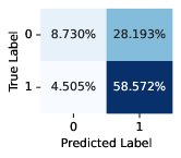
(c) SVM

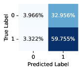
(d) SVM

(e) GB

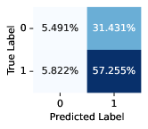
(f) GB

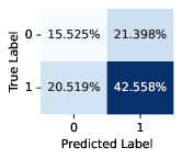
(g) MLP

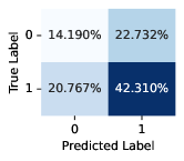
(h) MLP

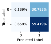
(i) RF

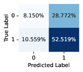
(j) RF

Figure 3.1: The confusion matrices for LR, SVM, GB, MLP, and RF via the TF-IDF (left-hand panels) and TF-IDF-VADER (right-hand panels) featurizations.

summarizes our classification results, with the meritorious complaints labeled as “0” and the anomalies (i.e., nonmeritorious complaints) labeled as “1”. The classification accuracy, which is the sum of the true positives (TP) and the true negatives (TN), as well as the percentage of complaints predicted as meritorious, which is the sum of the false positives (FP) and the true negatives (TN), are reported in Table 3.2

Model	TF-IDF			TF-IDF-VADER
	Accuracy	Merit		Accuracy	Merit
LR	67.37%	15.41%		63.96%	8.52%
SVM	67.30%	13.24%		63.72%	7.29%
GB	64.61%	16.43%		62.75%	11.31%
MLP	58.08%	36.04%		56.50%	34.96%
RF	65.56%	9.80%		60.67%	18.71%

Table 3.2: Classification accuracy (TP+TN) and the percentage of complaints predicted as meritorious (FP+TN) for the TF-IDF and TF-IDF-VADER featurizations.

for the five classification methods. Note that the TF-IDF featurization consistently generates higher accuracy than the TF-IDF-VADER featurization.

4 Converting narratives into quantitative data

We now introduce several economics-based quantities and equations needed to construct two anomaly detection indices in Section 6. The indices require to convert the narratives of consumer complaints into quantitative data. We establish a conversion mechanism with the help of word counts of the cleaned narratives, discounted dollar amounts obtained via the CPI as described earlier, and VADER sentiment intensities (Hutto and Gilbert, 2014).

4.1 TF-IDF approach

To measure the sentiment level for the analysis of CFPB consumer complaints, we employ the VADER function $\textrm{VADER}\mathrel{\mathop{\mathchar 58\relax}}\Omega\to[-4,4]$ with $\Omega$ denoting the Bag of Words of the VADER sentiment lexicon, that has been widely used in finance (e.g., Osman and Sabit, 2022; Long et al., 2023), public health (e.g., Sanders et al., 2021), and other research areas. Namely, for each consumer $i$, we define the sentiment score

$$s_{i}=\sum_{w_{j}\textrm{ in both }d_{j}\textrm{ and }W_{-}}\big{|}\textrm{VADER}(w_{j})\big{|},$$ (4.1)

where the sum is taken over all words $w_{j}$ that are both in the cleaned narrative $d_{i}$ and in the set $W_{-}$ of those words that have negative VADER sentiment intensities. Hence, we can rewrite the sentiment score $s_{i}$ as follows:

$$s_{i}=\sum_{w_{j}\textrm{ in }d_{j}}\mathds{1}\{\textrm{VADER}(w_{j})<0\}\big{(}-\textrm{VADER}(w_{j})\big{)},$$

where $\mathds{1}$ denotes the indicator function. It is instructive to compare this sentiment score with the one used by Osman and Sabit (2022).

The time and effort invested by the consumer $i$ to generate a complaint depend on 1) how much money the consumer was charged, or how much return the consumer has not received, and 2) the consumer’s sentiment level due to lost money. With the number $m_{i}^{\textrm{TI}}$ of words in the cleaned narrative $d_{i}$, the adjusted dollar amount $l_{i}$, and the sentiment score $s_{i}$, we assume the Cobb-Douglas equation

$$m_{i}^{\textrm{TI}}=\beta s_{i}^{\alpha}l_{i}^{1-\alpha},$$ (4.2)

where $\alpha\in(0,1)$ is a geometric weight and $\beta>0$ is a scale factor. Note that by the Cobb-Douglas equation, the law of diminishing marginal utility is satisfied for the sentiment score $s_{i}$ and the adjusted dollar amount $l_{i}$.

Note 4.1.

Since $\textrm{VADER}(w)\in[-4,4]$ for every word $w$ (Hutto and Gilbert, 2014), the sentiment scores $s_{i}$ are non-negative and do not exceed $4m_{i}^{\textrm{TI}}$. Hence, $s_{i}/(4m_{i}^{\textrm{TI}})\in[0,1]$. This fact will play a role in the following sections.

By taking the logarithms of the two sides of equation (4.2), we obtain

$$\log\bigg{(}{m_{i}^{\textrm{TI}}\over l_{i}}\bigg{)}=\alpha\log\bigg{(}{s_{i}\over l_{i}}\bigg{)}+\log(\beta).$$ (4.3)

We can now estimate the parameter $\alpha$ using simple linear regression, which gives

$$\hat{\alpha}=0.990 (0.983,0.997)$$ with the 95% confidence interval . (4.4)

The resulting scatter-plot, which is based on the points

$$\bigg{(}\log\bigg{(}{s_{i}\over l_{i}}\bigg{)},\log\bigg{(}{m_{i}^{\textrm{TI}}\over l_{i}}\bigg{)}\bigg{)},\quad i=1,\dots,2,849,$$ (4.5)

as well as the fitted least squares regression line are depicted in Figure 4.1.

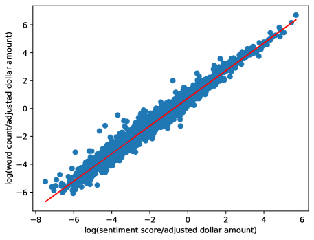
Figure 4.1: Scatter-plot (4.5) and to it fitted least squares regression line.

The diagnostic plots for this linear model are in Figure 4.2.

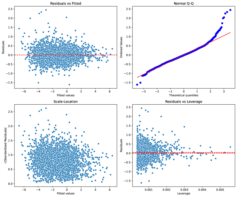
Figure 4.2: Diagnostic plots for model (4.3).

Note that the 95% confidence interval $(0.983,0.997)$ is included in $(0.5,1)$. Hence we can say that equation (4.2) holds for some $\alpha\in(0.5,1)$.

4.2 TF-IDF-VADER approach

With the number $m_{i}^{\textrm{TIV}}$ of those words that are both in the cleaned narrative $d_{i}$ and in the set $W_{-}$, the adjusted dollar amount $l_{i}$, and the sentiment score $s_{i}$ defined by equation (4.1), we assume the Cobb-Douglas equation

$$m_{i}^{\textrm{TIV}}=\beta s_{i}^{\alpha}l_{i}^{1-\alpha}.$$ (4.6)

Naturally, being based on the TF-IDF-VADER approach rather than TF-IDF, this equation leads to different estimates of the geometric weight $\alpha\in(0,1)$ and the scale factor $\beta>0$ than those obtained from equation (4.2). As we shall see in next Section 5, these estimates will give rise to different shapes of the input-output system’s transfer functions.

Note 4.2.

Since the sentiment score $s_{i}$ is non-negative and does not exceed $4m_{i}^{\textrm{TIV}}$, we have $s_{i}/(4m_{i}^{\textrm{TIV}})\in[0,1]$. This fact will play a role in the following sections.

By taking the logarithms of the two sides of equation (4.6), we obtain

$$\log\bigg{(}{m_{i}^{\textrm{TIV}}\over l_{i}}\bigg{)}=\alpha\log\bigg{(}{s_{i}\over l_{i}}\bigg{)}+\log(\beta).$$ (4.7)

We estimate the parameter $\alpha$ using simple linear regression, which gives

$$\hat{\alpha}=1.004 (1.001,1.007)$$ with the 95% confidence interval . (4.8)

The resulting scatter-plot, which is based on the points

$$\bigg{(}\log\bigg{(}{s_{i}\over l_{i}}\bigg{)},\log\bigg{(}{m_{i}^{\textrm{TIV}}\over l_{i}}\bigg{)}\bigg{)},\quad i=1,\dots,2,849,$$ (4.9)

as well as the fitted least squares regression line are depicted in Figure 4.3.

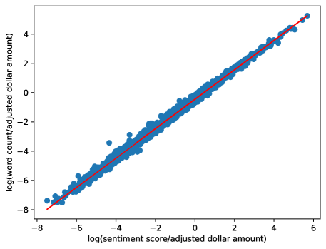
Figure 4.3: Scatter-plot (4.9) and to it fitted least squares regression line.

The diagnostic plots for this linear model are in Figure 4.4.

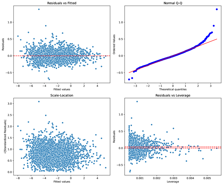
Figure 4.4: Diagnostic plots for model (4.7).

Note that the 95% confidence interval $(1.001,1.007)$ suggests that equation (4.6) holds for some $\alpha>1$.

5 The input-output systems

Training anomaly detection classifiers leads to confusion matrices involving classification errors, and it also generates a meritorious subset of observations. In addition to being classified as meritorious, the observations within the meritorious set are expected to follow equation (4.6), which leads to an input-output system specific for a chosen featurization, as we shall describe next.

5.1 The TF-IDF approach

We first rewrite equation (4.2) as

$$\left(\frac{s_{i}}{m_{i}^{\textrm{TI}}}\right)^{\alpha}\left(\frac{l_{i}}{m_{i}^{\textrm{TI}}}\right)^{1-\alpha}=\frac{1}{\beta},$$

from which we obtain

$$\log(y_{i}^{\textrm{TI}})=\frac{\alpha}{1-\alpha}\log(x_{i}^{\textrm{TI}})+c_{1}$$ (5.1)

with the outputs

$$y_{i}^{\textrm{TI}}={m_{i}^{\textrm{TI}}\over l_{i}},$$ (5.2)

the inputs (recall Note 4.1)

$$x_{i}^{\textrm{TI}}={s_{i}\over 4m_{i}^{\textrm{TI}}}\in[0,1],$$ (5.3)

and the constant

$$c_{1}=\frac{\alpha}{1-\alpha}\log(4)+\frac{1}{1-\alpha}\log(\beta).$$

Equation (5.1) establishes the input-output relationship

$$y_{i}^{\textrm{TI}}=h_{0}(x_{i}^{\textrm{TI}})$$

with the transfer function

$$h_{0}(x)=c_{2}x^{\alpha/(1-\alpha)},$$ (5.4)

where

$$c_{2}=e^{c_{1}}.$$

Since $x_{i}^{\textrm{TI}}\in[0,1]$, the domain of definition of $h_{0}$ is the unit interval $[0,1]$.

The notion of transfer function plays a pivotal role in the application of the anomaly detection method developed by Gribkova and Zitikis (2018, 2019a, 2019b, 2020) and Sun et al. (2022). Its importance will be seen in the next section. Related specifically to function (5.4), its first derivative is

$$h_{0}^{\prime}(x)=c_{3}x^{(2\alpha-1)/(1-\alpha)}$$

for a constant $c_{3}$. Hence, since we have assumed $\alpha\in(0.5,1)$ based on result (4.4), and since the inputs are in $[0,1]$, the derivative $h_{0}^{\prime}$ is bounded on the interval $[0,1]$. Therefore, the transfer function $h_{0}$ is Lipschitz continuous on $[0,1]$. This is an important property as seen from Sun et al. (2022, Theorem 1 (i)).

5.2 The TF-IDF-VADER approach

Analogously to Section 5.1, we obtain the input-output relationship

$$y_{i}^{\textrm{TIV}}=h_{0}(x_{i}^{\textrm{TIV}})$$

with the same transfer function $h_{0}$ and the analogously defined inputs

$$x_{i}^{\textrm{TIV}}={s_{i}\over 4m_{i}^{\textrm{TIV}}}\in[0,1]$$ (5.5)

and outputs

$$y_{i}^{\textrm{TIV}}={m_{i}^{\textrm{TIV}}\over l_{i}}.$$ (5.6)

Note, however, that in view of result (4.8), we need to conclude $\alpha>1$, in which case the transfer function

$$h_{0}(x)=c_{2}x^{\alpha/(1-\alpha)}\leavevmode\nobreak\ \bigg{(}={c_{2}\over x^{\alpha/(\alpha-1)}}\bigg{)}$$

is not Lipschitz continuous on the interval $[0,1]$. Fortunately, it satisfies another set of conditions of Sun et al. (2022, Theorem 1 (ii)) enabling us to apply the anomaly detection method.

6 Anomaly detection among quantified narratives

In the ideal scenario, the pairs $(x_{i},y_{i})$, which are either $(x_{i}^{\textrm{TI}},y_{i}^{\textrm{TI}})$ or $(x_{i}^{\textrm{TIV}},y_{i}^{\textrm{TIV}})$ depending on the featurization used, for those $i$’s in the predicted meritorious set form an anomaly-free input-output system. In reality, however, anomalies are inevitable for input-output systems that are not particularly stringent, and they may even be present in the data due to the very nature of the problem. Such anomalies may not change the regime of inputs and/or outputs, and may therefore be difficult to detect for typical classifiers.

For this reason, we next construct two indices based on the pairs $(x_{i},y_{i})$ within the predicted meritorious set. For the purpose, we adapt the method for systematic-anomaly detection developed by Gribkova and Zitikis (2018, 2019a, 2019b, 2020) in the case of (quantitative) i.i.d. inputs and subsequently extended to time series inputs by Sun et al. (2022).

6.1 The $I$-index and findings

Let a simple random sample of pairs $(x_{1},y_{1}),\dots,(x_{n},y_{n})$ form an input-output system, where the inputs $x_{i}$ and the outputs $y_{i}$ are assumed to be coming from continuous random variables. Suppose that there are no ties among $x_{1},\ldots,x_{n}$, in which case we order the inputs in a unique way and obtain the values $x_{1\mathrel{\mathop{\mathchar 58\relax}}n}<x_{2\mathrel{\mathop{\mathchar 58\relax}}n}<\cdots<x_{n\mathrel{\mathop{\mathchar 58\relax}}n}$. We denote the corresponding concomitants (see, e.g., David and Nagaraja, 2003) of the outputs $y_{1},\ldots,y_{n}$ by $y_{1,n},\dots,y_{n,n}$.

Relying on the theory developed by Gribkova and Zitikis (2018, 2019a, 2019b, 2020) and Sun et al. (2022), the presence of systematic anomalies among the observed pairs can be assessed by the rate of convergence to $1/2$ of the $I$-index

$$I_{n}={\sum^{n}_{i=2}\big{(}y_{i,n}-y_{i-1,n}\big{)}_{+}\over\sum^{n}_{i=2}\big{|}y_{i,n}-y_{i-1,n}\big{|}},$$

where $a_{+}$ denotes the positive part of any real number $a$, that is, $a_{+}=a$ when $a>0$ and $a_{+}=0$ when $a\leq 0$.

The $I$-index appeared in Davydov and Zitikis (2017) as the solution to an optimization problem. It was further explored by Chen et al. (2018) and subsequently extended to the multivariate case by Davydov et al. (2019) to accommodate the diverse needs of applications. The index has found uses in, e.g., education sciences (Chen and Zitikis, 2017), but most notably in various branches of engineering and related areas, such as system security (Gribkova and Zitikis, 2019a, 2020), anomaly detection (Sun et al., 2022), electrical engineering (Chernov et al., 2021; Di Capua et al., 2023a, b; Milano et al., 2023) mechanical and materials engineering (Kirk, 2020; Kirk et al., 2021; Sauceda et al., 2022), networks (Gurfinkel, 2020; Gurfinkel and Rikvold, 2020), and prognostics (Trilla et al., 2020).

Applying Algorithm 6.1

Require

1. A dataset $D$ with labels “meritorious” and “nonmeritorious”.

2. A specific classification method.

Compute a value of the $I$-index

1. Randomly assign $(1-r)100\%$ of the dataset $D$ as a training set, and the remaining

$r100\%$ as a testing set.

2. Train a classifier $f$ using the specific classification method based on the training set.

3. Apply $f$ on the testing set, leading to a meritorious subset with the indices $d_{m}\subseteq D$ of

the testing set.

4. Compute the $I$-index using $(x_{i},y_{i})$, $i\in d_{m}$.

Algorithm 6.1: Calculating the $I$-index.

on each of the predicted meritorious set generated by the five classifiers, we obtain Figure 6.1

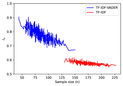
(a) LR

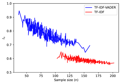
(b) SVM

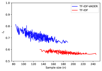
(c) GB

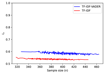
(d) MLP

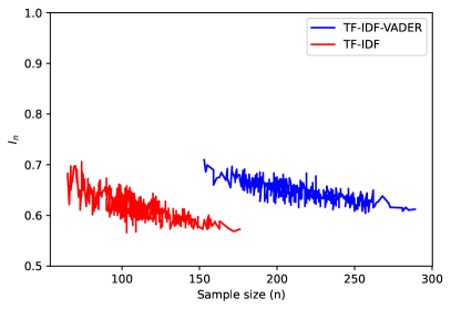
(e) RF

Figure 6.1: The plots of $I_{n}$ for the five classifications.

depicting the $I$-index for each of the five classifiers. In Algorithm 6.1, we have set the parameter $r$ to $0.4$.

Note that for these classifiers except MLP, the graphs seem to rapidly move in the direction of $1/2$, although we cannot say with certainty that they would reach $1/2$ had the sample sizes been much larger. At any rate, given what we see now, we would conclude the presence of systematic anomalies. As to the MLP classifier, it is difficult to claim from the nearly flat graphs in the case of both featurizations that there is a tendency to convergence to $1/2$, although it could be so but at a very slow rate. If we think that there is no convergence to $1/2$, then given the properties of the $I$-index, we conclude that the input-output system is anomaly free.

Given the aforementioned ambiguities, it is prudent to have a supplementary view. This leads to the next section concerning the $B$-index and its behaviour.

6.2 The $B$-index and findings

To introduce the $B$-index, we first note that for any real number $a$, we can express its positive part $a_{+}$ as $(a+|a|)/2$. Since $\sum^{n}_{i=2}\big{(}y_{i,n}-y_{i-1,n}\big{)}=y_{n,n}-y_{1,n}$, we therefore have

$$I_{n} ={\sum^{n}_{i=2}\big{(}y_{i,n}-y_{i-1,n}\big{)}_{+}\over\sum^{n}_{i=2}\big{|}y_{i,n}-y_{i-1,n}\big{|}}$$

$$={1\over 2}\bigg{(}1+{y_{n,n}-y_{1,n}\over\sum^{n}_{i=2}\big{|}y_{i,n}-y_{i-1,n}\big{|}}\bigg{)}.$$

In view of this representation of the $I$-index, the convergence of $I_{n}$ to $1/2$ is associated with the stochastic growth to infinity of the sum

$$S_{n}=\sum^{n}_{i=2}\big{|}y_{i,n}-y_{i-1,n}\big{|}$$

when $n\to\infty$. We have depicted this sum as a function of $n$ in Figure 6.2

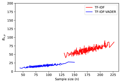
(a) LR

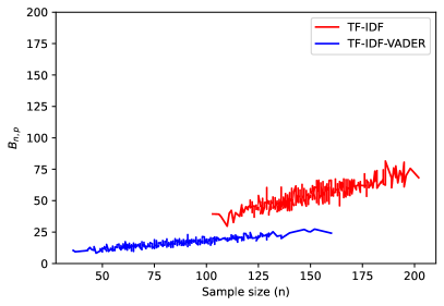
(b) SVM

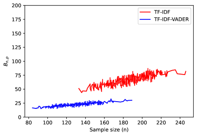
(c) GB

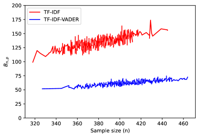
(d) MLP

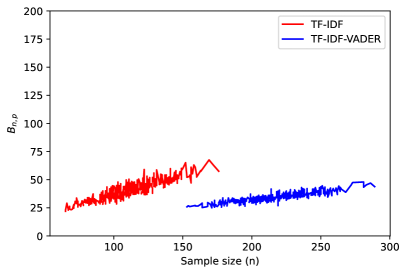
(e) RF

Figure 6.2: The plots of $S_{n}$ for the five classifications.

for the five classifications. To produce the figure, we have followed Algorithm 6.1 with $S_{n}$ instead of $I_{n}$, setting the parameter $r$ to $0.4$. For the purpose of comparison, the vertical axes in all the five panels of the figure are the same and run from $0$ to $200$.

To parameterize the stochastic growth of the sum $S_{n}$ to infinity when $n$ increases, we use the $B$-index

$$B_{n,p}={1\over n^{1/p}}\sum^{n}_{i=2}\big{|}y_{i,n}-y_{i-1,n}\big{|}\leavevmode\nobreak\ \bigg{(}={S_{n}\over n^{1/p}}\bigg{)},$$

where $p\in(0,\infty]$ is a parameter. The normalization $n^{1/p}$ mimics that of the law of large numbers when $p=1$ and that of the central limit theorem when $p=2$. In the extreme case $p=\infty$, the normalization becomes identical to $1$, and thus the $B$-index reduces to $S_{n}$.

By varying the parameter $p$ values, we can get sense of the growth to infinity of $S_{n}$ when $n\to\infty$. This is linked to the notion of reasonable order. Specifically, we say that the outputs are in $p$-reasonable order with respect to the inputs for some $p$ if $B_{n,p}$ is stochastically bounded when $n\to\infty$. Otherwise, that is, when $B_{n,p}$ stochastically grows to infinity when $n\to\infty$, the outputs are said to be out of $p$-reasonable order. This notion of in/out of $p$-reasonable order in the case $p=2$ was introduced by Gribkova and Zitikis (2018, 2019a, 2019b, 2020) and subsequently extended to arbitrary $p\in(0,\infty]$ by Sun et al. (2022) to accommodate a whole spectrum of tail heaviness in time series data.

By Sun et al. (2022, Theorem 4), the anomaly-free outputs are in $p$-reasonable order for $p=\infty$ and therefore for all $p\in(0,\infty]$. For any two parameter values $p_{1}<p_{2}$, the outputs, which may contain anomalies, can be out of $p_{2}$-reasonable order but in $p_{1}$-reasonable order. Hence, by visualizing the behaviour of $B_{n,p_{1}}$ and $B_{n,p_{2}}$ with respect to various sample sizes $n$, we can develop an understanding of when, with respect to $p$, the meritorious set becomes in, or out of, $p$-reasonable order. For this task, we follow Algorithm 6.1 with $B_{n,p}$ instead of $I_{n}$. We do so $k=500$ times and obtain $k$ values of the $B$-index, always setting the parameter $r$ to $0.4$.

Figures A.1–A.5, which are relegated to Appendix A due to space considerations, depict the $B$-indices arising from the TF-IDF and TF-IDF-VADER featurizations. For the purpose of comparison, the vertical axes in all the panels of the figures are the same and run from $0$ to $5$. We observe that in the case of both featurizations and for every classification method, when the parameter $p$ decreases, that is, when its reciprocal $1/p$ goes through the values $0.6$, $0.7$, $0.8$ and $0.9$, the meritorious sets shift at some point from being out of $p$-reasonable order to being in $p$-reasonable order. This pattern is, of course, natural as the normalizing factor $n^{1/p}$ gets heavier for larger $1/p$, thus slackening the growth of the sum $S_{n}$ when systematic anomalies are present.

We see from Figures A.1–A.3, which refer to the LR, SVM, and GB classifications, that the TF-IDF featurization generally leads to larger sample sizes than the TF-IDF-VADER featurization. In the case of the MLP classification, we see from Figure A.4 that the sample sizes, in general, become similar. In the case of the RF classification, as seen from Figure A.5, it is the TF-IDF-VADER featurization that generally leads to larger sample sizes than the TF-IDF featurization.

Note also from Figures A.1–A.5 that in the case of the TF-IDF featurization, the system tends to shift from out of $0.7^{-1}$-reasonable order to in $0.8^{-1}$-reasonable order, whereas in the case of the TF-IDF-VADER featurization, we observe the tendency to shift from out of $0.6^{-1}$-reasonable order to in $0.7^{-1}$-reasonable order.

To formally check if the resulting meritorious set is in $p$-reasonable order, we define $p^{*}$ as the largest $p\geq 1$ such that the $B$-index $B_{n,p}$ is stochastically bounded when $n\to\infty$. Of course, depending on the featurization, there are two $p^{*}$’s: one is $p^{*}_{\text{TI}}$ arising from the TF-IDF featurization, and the second one is $p^{*}_{\text{TIV}}$ arising from the TF-IDF-VADER featurization. Given our observations, we roughly have

$$p^{*}_{\text{TI}}\in(0.8^{-1},0.7^{-1})\quad\textrm{and}\quad p^{*}_{\text{TIV}}\in(0.7^{-1},0.6^{-1})$$

for all the five classification methods. This implies $p^{*}_{\text{TIV}}>p^{*}_{\text{TI}}$ regardless of the classification method and suggests that there exists $p^{\prime}\in(p^{*}_{\text{TI}},p^{*}_{\text{TIV}})$ such that, for any given classification method, the $B$-index $B_{n,p^{\prime}}$ is stochastically bounded if the TF-IDF-VADER featurization is used but stochastically grows to infinity if the TF-IDF featurization is used. Therefore, the TF-IDF-VADER featurization leads to a relatively higher extent of anomaly absence because the $B$-index $B_{n,p^{\prime}}$ rejects the TF-IDF case as being anomaly free but cannot reject the TF-IDF-VADER case as being such. Finally, we note that when making these interpretations, we keep in mind that smaller $p^{*}$’s suggest heavier anomalies in the system, as smaller $p^{*}$’s give rise to larger $(1/p)$’s ($p<p^{*}$), thus producing heavier normalizing factors $n^{1/p}$ needed to slacken the growth of the sum $S_{n}$ with respect to $n\to\infty$.

7 Conclusion

We have proposed a method for detecting systematic anomalies among texts such as consumer complaint narratives. In addition to classification algorithms, quantitative indices have been employed to assists in anomaly detection. The index is essential for detecting those anomalies that mimic meritorious complaints without changing the distributional patterns of the word counts, discounted dollar amounts, and sentiment scores. It also plays a pivotal role when automating the procedure. Repeated classifications on randomly segmented training and testing datasets have been employed to visualise the index performance in different scenarios.

All the procedural steps have been illustrated using consumer complaints from the Consumer Complaint Database of the Consumer Financial Protection Bureau. Our results have shown that the TF-IDF-VADER featurization outperforms the TF-IDF featurization in terms of the indices $I_{n}$ and $B_{n,p}$ regardless of the chosen classification method, although the TF-IDF featurization consistently leads to slightly higher classification accuracy than the TF-IDF-VADER featurization. This suggest that, in practice, the TF-IDF-VADER featurization could be applied to consumer complaints to identify those with higher priority to receive reliefs, because the resulting meritorious group is less likely to contain nonmeritorious complaints.

Appendix A Graphs of the $B$-index

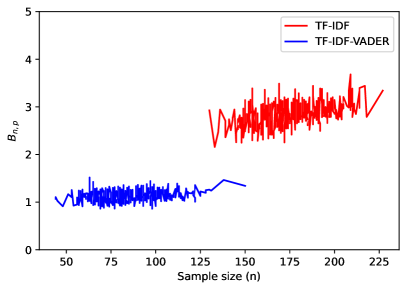
(a) $p=0.6^{-1}$

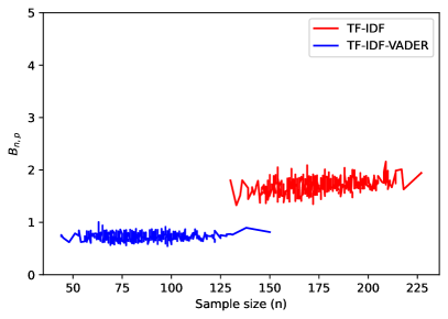
(b) $p=0.7^{-1}$

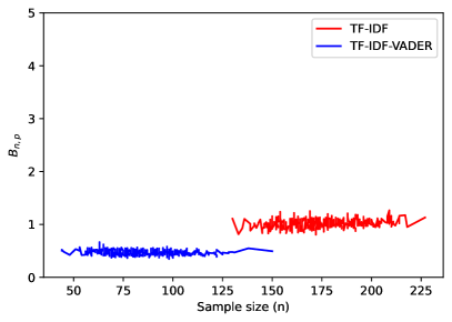
(c) $p=0.8^{-1}$

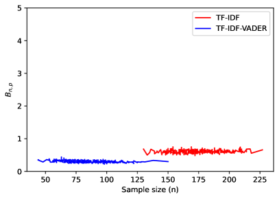
(d) $p=0.9^{-1}$

Figure A.1: The plots of $B_{n,p}$ (vertical axis) for various sample sizes $n$ (horizontal axis) and parameter $p$ values when using the LR classification.

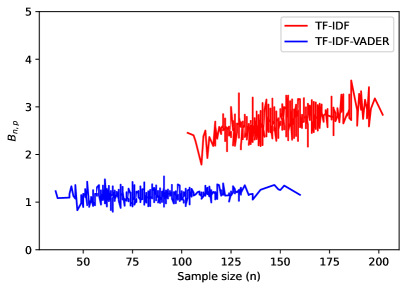
(a) $p=0.6^{-1}$

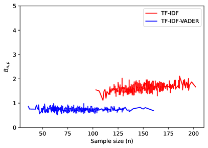
(b) $p=0.7^{-1}$

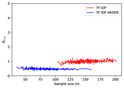
(c) $p=0.8^{-1}$

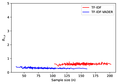
(d) $p=0.9^{-1}$

Figure A.2: The plots of $B_{n,p}$ (vertical axis) for various sample sizes $n$ (horizontal axis) and parameter $p$ values when using the SVM classification.

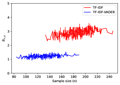
(a) $p=0.6^{-1}$

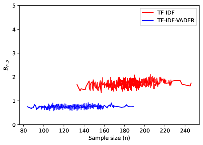
(b) $p=0.7^{-1}$

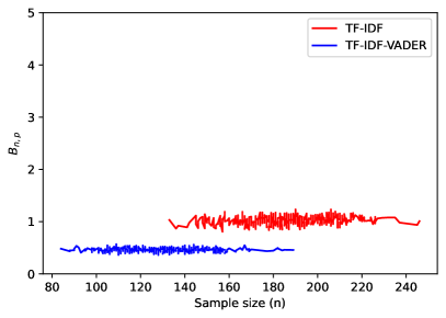
(c) $p=0.8^{-1}$

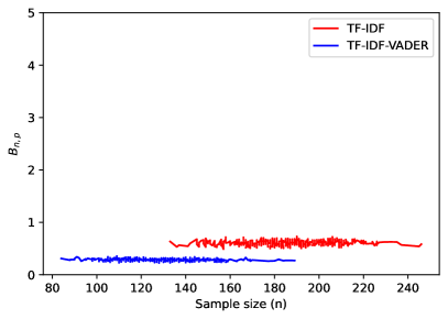
(d) $p=0.9^{-1}$

Figure A.3: The plots of $B_{n,p}$ (vertical axis) for various sample sizes $n$ (horizontal axis) and parameter $p$ values when using the GB classification.

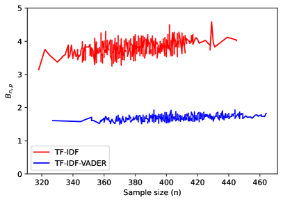
(a) $p=0.6^{-1}$

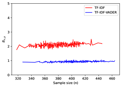
(b) $p=0.7^{-1}$

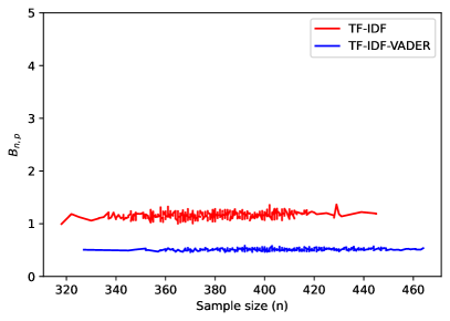
(c) $p=0.8^{-1}$

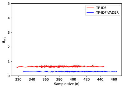
(d) $p=0.9^{-1}$

Figure A.4: The plots of $B_{n,p}$ (vertical axis) for various sample sizes $n$ (horizontal axis) and parameter $p$ values when using the MLP classification.

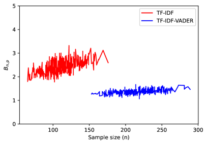
(a) $p=0.6^{-1}$

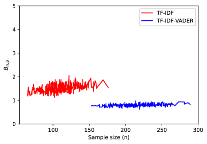
(b) $p=0.7^{-1}$

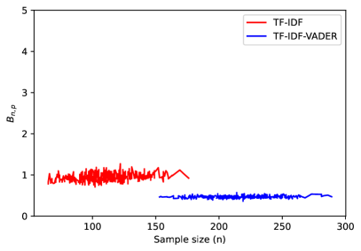
(c) $p=0.8^{-1}$

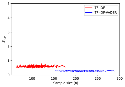
(d) $p=0.9^{-1}$

Figure A.5: The plots of $B_{n,p}$ (vertical axis) for various sample sizes $n$ (horizontal axis) and parameter $p$ values when using the RF classification.

References

- Bollacker et al. (1998) Bollacker, K.D., Lawrence, S. and Giles, C.L. (1998). CiteSeer: an autonomous web agent for automatic retrieval and identification of interesting publications. Proceedings of the Second International Conference on Autonomous Agents, 116-123.
-
CFPB (2023)
CFPB (2023).
Consumer Complaint Database. Consumer Financial Protection Bureau, Washington, DC.
https://urldefense.proofpoint.com/v2/url?u=https-3A__www.consumerfinance.gov_data-2Dresearch_consumer-2Dcomplaints_&d=DwIGaQ&c=shNJtf5dKgNcPZ6Yh64b-ALLUrcfR-4CCQkZVKC8w3o&r=TOYNRvr5iRnx_eTG1f9w9tvM8r-PRRjoTxFmf1MCaYc&m=zugDJhYhWpfVunt6SYNWrDD_UWvP1kTMSFSYKzCbeFKS5g_YTxCdU1XjTiR1WIE_&s=aiIWJJb637yIrIjfkls9T9x23ejON6Q7YoEPwHvhA8Q&e=. -
CPI (2023)
CPI (2023).
Consumer Price Index, 1913-. Federal Reserve Bank of Minneapolis, Mineapolis, MN.
https://urldefense.proofpoint.com/v2/url?u=https-3A__www.minneapolisfed.org_about-2Dus_monetary-2Dpolicy_inflation-2Dcalculator_consumer-2Dprice-2Dindex-2D1913-2D&d=DwIGaQ&c=shNJtf5dKgNcPZ6Yh64b-ALLUrcfR-4CCQkZVKC8w3o&r=TOYNRvr5iRnx_eTG1f9w9tvM8r-PRRjoTxFmf1MCaYc&m=zugDJhYhWpfVunt6SYNWrDD_UWvP1kTMSFSYKzCbeFKS5g_YTxCdU1XjTiR1WIE_&s=wXpLT2Qtyb2S5SxBhgzB6UuTL1onm6CVfu2yiKCPMZE&e=. - Chen et al. (2018) Chen, L., Davydov, Y., Gribkova, N. and Zitikis, R. (2018). Estimating the index of increase via balancing deterministic and random data. Mathematical Methods of Statistics, 27, 83–102.
- Chen and Zitikis (2017) Chen, L. and Zitikis, R. (2017). Measuring and comparing student performance: a new technique for assessing directional associations. Education Sciences, 7, 1–27 (article #77).
- Chernov et al. (2021) Chernov, N.I., Butyrlagin, N.V., Prokopenko, N.N. and Yugai, V.Y. (2021). Synthesis and circuitry of multi-valued digital current logic elements: “classical” linear-monotonic approach. International Conference on Electrical Engineering and Photonics (EExPolytech), St. Petersburg, Russian Federation, 2021, pp. 104-107,
- David and Nagaraja (2003) David, H.A. and Nagaraja, H.N. (2003). Order Statistics. (Third Edition.) Wiley, Hoboken.
- Davydov et al. (2019) Davydov, Y., Moldavskaya, E. and Zitikis, R. (2019). Searching for and quantifying nonconvexity regions of functions. Lithuanian Mathematical Journal (Special issue dedicated to Professor Vygantas Paulauskas on the occasion of his 75th birthday), 59, 507–518.
- Davydov and Zitikis (2017) Davydov, Y. and Zitikis, R. (2017). Quantifying non-monotonicity of functions and the lack of positivity in signed measures. Modern Stochastics: Theory and Applications, 4, 219–231.
- Di Capua et al. (2023a) Di Capua, G., Bourelly, C., De Stefano, C., Fontanella, F., Milano, F., Molinara, M., Oliva, N. and Porpora, F. (2023). Using genetic programming to learn behavioral models of lithium batteries. In: Correia, J., Smith, S. and Qaddoura, R. (eds) Applications of Evolutionary Computation. EvoApplications. Lecture Notes in Computer Science, vol 13989, pp. 461–474. Springer, Cham.
- Di Capua et al. (2023b) Di Capua, G., Oliva, N., Milano, F., Bourelly, C., Porpora, F., Maffucci, A. and Femia, N. (2023). A behavioral model for lithium batteries based on genetic programming. IEEE International Symposium on Circuits and Systems (ISCAS), Monterey, CA, USA, pp. 1–5.
- Di Vincenzo et al. (2023) Di Vincenzo, D., Greselin, F., Piacenza, F. and Zitikis, R. (2023). A text analysis of operational risk loss descriptions. Journal of Operational Risk, 18, 63–90.
- Gribkova and Zitikis (2018) Gribkova, N. and Zitikis, R. (2018). A user-friendly algorithm for detecting the influence of background risks on a model. Risks (Special issue on “Risk, Ruin and Survival: Decision Making in Insurance and Finance”), 6, 1–11. (Article #100.)
- Gribkova and Zitikis (2019a) Gribkova, N. and Zitikis, R. (2019a). Assessing transfer functions in control systems. Journal of Statistical Theory and Practice, 13, 1–33. (Article #35.)
- Gribkova and Zitikis (2019b) Gribkova, N. and Zitikis, R. (2019b). Statistical detection and classification of background risks affecting inputs and outputs. Metron – International Journal of Statistics, 77, 1–18.
- Gribkova and Zitikis (2020) Gribkova, N. and Zitikis, R. (2020). Detecting intrusions in control systems: a rule of thumb, its justification and illustrations. Journal of Statistics and Management Systems, 23, 1285–1304.
- Gurfinkel (2020) Gurfinkel, A.J. (2020). Centrality Reach and Grasp: Analyzing the Attenuation of Influence Flows in Parametrized Centrality Measures on Complex Networks. Ph.D. Thesis. The Florida State University, Florida.
- Gurfinkel and Rikvold (2020) Gurfinkel, A.J. and Rikvold, P.A. (2020). Absorbing random walks interpolating between centrality measures on complex networks. Physical Review E, 101, 1–21, Article 012302.
- Hayes et al. (2021) Hayes, R.M., Jiang, F. and Pan, Y. (2021). Voice of the customers: Local trust culture and consumer complaints to the CFPB. Journal of Accounting Research, 59, 1077–1121.
- Hutto and Gilbert (2014) Hutto, C. and Gilbert, E. (2014). Vader: A parsimonious rule-based model for sentiment analysis of social media text. Proceedings of the International AAAI Conference on Web and Social Media, 8, 216–225.
- Ji et al. (2023) Ji, Z., Duan, X., Pons, D., Chen, Y. and Pei, Z. (2023). Integrating text mining and analytic hierarchy process risk assessment with knowledge graphs for operational risk analysis. Journal of Operational Risk, 18, 31–61.
- Karami and Pendergraft (2018) Karami, A. and Pendergraft, N.M. (2018). Computational Analysis of Insurance Complaints: Geico Case Study. Available at arXiv:1806.09736
- Kirk (2020) Kirk, T.Q. (2020). Computational Design of Compositionally Graded Alloys. Ph.D. Thesis. Texas A&M University, Texas.
- Kirk et al. (2021) Kirk, T., Malak, R. and Arroyave, R. (2021). Computational design of compositionally graded alloys for property monotonicity. Journal of Mechanical Design, 143, Article #031704 (9 pages).
- Klein (1995) Klein, R.W. (1995). Insurance regulation in transition. Journal of Risk and Insurance, 62, 363–404.
- Liao et al. (2020) Liao, X., Chen, G., Ku, B., Narula, R. and Duncan, J. (2020). Text mining methods applied to insurance company customer calls: a case study. North American Actuarial Journal, 24, 153–163.
- Littwin (2014) Littwin, A. (2014). Why process complaints? Then and now. Temple Law Review, 87, 895–946.
- Long et al. (2023) Long, S., Lucey, B., Xie, Y. and Yarovaya, L. (2023). “I just like the stock”: The role of Reddit sentiment in the GameStop share rally. Financial Review, 58, 19–37.
- Milano et al. (2023) Milano, F., Di Capua, G., Oliva, N., Porpora, F., Bourelly, C., Ferrigno, L. and Laracca, M. (2023). An analytical model for lithium-ion batteries based on genetic programming approach. IEEE International Workshop on Metrology for Automotive (MetroAutomotive), Modena, Italy, pp. 35–40.
-
NAIC (2022)
NAIC (2022).
2021 Insurance Department Resources Report, Volume 1.
National Association of Insurance Commissioners, Washington, DC.
https://urldefense.proofpoint.com/v2/url?u=https-3A__content.naic.org_sites_default_files_publication-2Dsta-2Dbb-2Dvolume-2Done.pdf&d=DwIGaQ&c=shNJtf5dKgNcPZ6Yh64b-ALLUrcfR-4CCQkZVKC8w3o&r=TOYNRvr5iRnx_eTG1f9w9tvM8r-PRRjoTxFmf1MCaYc&m=zugDJhYhWpfVunt6SYNWrDD_UWvP1kTMSFSYKzCbeFKS5g_YTxCdU1XjTiR1WIE_&s=EXzb1f5bnSijwBHoMrH0sJ3htPF2Ehm01LtLwOitupI&e=. -
NAIC (2023)
NAIC (2023).
Insurance Departments.
National Association of Insurance Commissioners, Washington, DC.
https://urldefense.proofpoint.com/v2/url?u=https-3A__content.naic.org_state-2Dinsurance-2Ddepartments&d=DwIGaQ&c=shNJtf5dKgNcPZ6Yh64b-ALLUrcfR-4CCQkZVKC8w3o&r=TOYNRvr5iRnx_eTG1f9w9tvM8r-PRRjoTxFmf1MCaYc&m=zugDJhYhWpfVunt6SYNWrDD_UWvP1kTMSFSYKzCbeFKS5g_YTxCdU1XjTiR1WIE_&s=GogQ3KH4X0fXnZxn-tmAnPL_BYDLqpdvePRaW9lsWxk&e= (accessed July 31, 2023). - Osman and Sabit (2022) Osman, S.M.I. and Sabit, A. (2022). Bank Scandal and Customer Sentiment. Available at SSRN 4035168.
- Pakhchanyan et al. (2022) Pakhchanyan, S., Fieberg, C., Metko, D. and Kaspereit, T. (2022). Machine learning for categorization of operational risk events using textual description. Journal of Operational Risk, 17, 37–65.
- Sanders et al. (2021) Sanders, A.C., White, R.C., Severson, L.S., Ma, R., McQueen, R., Paulo, H.C.A., Zhang, Y., Erickson, J.S. and Bennett, K.P. (2021). Unmasking the conversation on masks: Natural language processing for topical sentiment analysis of COVID-19 Twitter discourse. AMIA Summits on Translational Science Proceedings, 555.
- Sauceda et al. (2022) Sauceda, D., Singh, P., Ouyang, G., Palasyuk, O., Kramer, M.J. and Arróyave, R. (2022). High throughput exploration of the oxidation landscape in high entropy alloys. Materials Horizons, 9, 2644–2663.
- Spärck Jones (1972) Spärck Jones, K. (1972). A statistical interpretation of term specificity and its application in retrieval. Journal of Documentation, 28, 11–21.
- Sun et al. (2022) Sun, N., Yang, C. and Zitikis, R. (2022). Detecting systematic anomalies affecting systems when inputs are stationary time series. Applied Stochastic Models in Business and Industry, 38, 512–544.
- Trilla et al. (2020) Trilla, A., Fernández, V. and Cabré, X. (2020). Enhancing railway pantograph carbon strip prognostics with data blending through a time-delay neural network ensemble. Annual Conference of the PHM Society, 12, 1–9.
- Wang et al. (2022) Wang, Y., Chang, Y. and Li, J. (2022). How does the pandemic change operational risk? Evidence from textual risk disclosures in financial reports. Journal of Operational Risk, 17, 1–24.
- Wood and Morris (2010) Wood, G.L. and Morris, R.L. (2010). Consumer complaints against insurance companies. Journal of Personal Finance, 9, 101–116.