Kinematics of the Milky way from the statistical analysis of the Gaia Data Release 3

Abstract

By analysing data from the Gaia Space Observatory, we have obtained precise basic characteristics of the collective motion of stars in a part of our galaxy. Our research is based on a statistical analysis of the motion of $33~{}146~{}122$ selected stars at a distance $\lesssim 6$ kpc from the Sun. Up to this distance, Gaia provides high statistics of stars with well-measured proper motion and parallax needed to determine the corresponding transverse velocity with sufficient precision. We obtained the velocity of the Sun $\left(U_{\odot},V_{\odot},W_{\odot}\right)=(10.5\pm 1,22.5\pm 3,7.5\pm 0.5)$ km/s relative to a set of nearby stars and the rotation velocity of the galaxy at different radii. For the radius of the Sun’s orbit, we obtained the velocity$\ V_{0}\approx 225$ km/s. We have shown that the various kinematic characteristics and distributions, which depend on the position in the galaxy, can be very well described in the studied region by a simple Monte-Carlo simulation model based on five parameters in the galactocentric reference frame. The optimal values of these parameters were determined by comparison with the data.

I Introduction

Our galaxy, the Milky Way (MW), is a unique laboratory for gravity research and for understanding the formation and evolution of galaxies. In recent years, the Gaia Space Observatory has acquired a huge amount of precise astrometric, photometric and spectroscopic data on stars in the MW. The analysis of these data has been the subject of many thousands of publications.

The full astrometric solution (angular positions, parallax and proper motion) provides the necessary input data to produce a kinematic map of the MW. In general, it encompasses various structures on different scales, from orbiting of small gravitationally bound systems, binaries and multiple-bound systems, to the streaming motions of stellar fields in galactic arms with various turbulences and fluctuations, to the collective rotation of the whole galactic disk with the galactic halo. The nature of the rotation suggests the presence of dark matter, which generates a substantial part of the galactic gravitational field.

Along with gravity, the formation and evolution of the stars themselves are also governed by the forces of the microworld (strong, electroweak - unified electromagnetic+weak) based on a well-verified Standard model. The nature and origin of dark matter at the microscopic level have not yet been explained.

Recent studies of the MW kinematics have shown accurate results on the MW rotation represented by the rotation curve bh ; ei ; mr ; re defined as the dependence of the orbital velocity on the radius. Other topics concern the detailed mapping of many kinematic substructures outside axial symmetry ga1 ; ka ; lo ; ra ; wa . Some other related important issues are addressed in bl ; ch ; je ; sch ; vi .

The main goal of the present study is to analyze the kinematic map of the MW in the spatial domain where the necessary data are obtained with sufficient precision. We show that this map can be well approximated in the Galactocentric reference frame by a triple (symmetric and asymmetric) Gaussian distribution, which depends on distance from the galactic plane and is defined by five free parameters determined from the data. In Sec. II describes our methodology. First, we define transformation relations between galactic and Galactocentric reference systems. In the former system the Gaia data are obtained and presented, the latter is suitable for simulation. Then the definition of the simulation model follows. In the last part of this section, we define the format of data sectors with additional cuts that will be used for the analysis. In Sec. III we present obtained results involving velocity distributions in different sectors of the galactic reference frame. Analysis of these distributions gives results on the local and orbital velocity of the Sun, different representations of the rotation curve (RC), and finally on the tuning of all free parameters of the simulation model. Then a comparison of the simulation with all relevant distributions follows. Obtained results and the agreement with the simulation model are discussed in more detail in Sec. IV. The comparison of obtained results with other available data is a part of the discussion.

II Methodology

II.1 Reference frames

Positions of sources in Gaia data are represented in angular galactic coordinates: longitude ($l$) and latitude ($b$). With the use of parallax, we can define also the distance $r$ of the source from the Sun. For our analysis also representation in Galactocentric coordinates will be useful. The relation between both reference frames is illustrated in Fig.1.

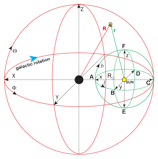
Figure 1: Galactic (green) and Galactocentric (red) reference frames

For simplicity, we assume the Sun is located in the galactic plane (its real position is slightly above the plane, $Z_{\odot}\approx 0.027$ kpc ch ). Then, the transformation between both the frames $\left(r,l,b\right)\rightarrow\left(R,\Phi,\Theta\right)$ is defined by equations:

$$R =\sqrt{r^{2}+R_{\odot}^{2}-2r_{0}R_{\odot}};\qquad r_{0}=r\cos l\cos b$$ (1)

$$\Theta =\arcsin\frac{r\sin b}{R}$$

$$\Phi =\arcsin\frac{r\sin l\cos b}{R\cos\Theta};\qquad r_{0}>R_{\odot}$$

$$\Phi =\pi-\arcsin\frac{r\sin l\cos b}{R\cos\Theta};\qquad r_{0}\leq R_{\odot}$$

and inversely $\left(R,\Phi,\Theta\right)\rightarrow$ $\left(r,l,b\right)$

$$r =\sqrt{R^{2}+R_{\odot}^{2}+2R_{0}R_{\odot}};\qquad R_{0}=R\cos\Phi\cos\Theta,$$ (2)

$$b =\arcsin\frac{R\sin\Theta}{r},$$

$$l =\pi-\arcsin\frac{R\sin\Phi\cos\Theta}{r\cos b};\qquad R_{0}>R_{\odot},$$

$$l =\arcsin\frac{R\sin\Phi\cos\Theta}{r\cos b};\qquad R_{0}\leq R_{\odot},$$

where $R_{\odot}$ is the distance of the Sun from the galactic center. The values obtained in the different recent measurements are in the interval $7.1-8.92$ kpc bl . For our analysis, we assume $R_{\odot}\approx 8$ kpc. We will need this transformation to model and simulate the motion of the stars in Sec.II.2. The axis of the galactic and Galactocentric reference frames are defined as

$$x =r\cos l\cos b,\ \ \ \ \ y=r\sin l\cos b,\ \ \ \ \ z=r\sin b,$$ (3)

$$X =R\cos\Phi\cos\Theta,\ \ \ \ \ Y=r\sin\Phi\cos\Theta,\ \ \ \ \ Z=r\sin\Theta,$$ (4)

which will be needed for analysis. So, the direction $x$ points to the centre of the galaxy and the direction $y$ is direction of the galaxy’s rotation. The corresponding coordinates are related as

$$X=x-R_{\odot};\qquad Y=y;\qquad Z=z.$$ (5)

The proper motion of the stars in Gaia data is represented by the vector

$$\mathbf{\mu}_{ICRS}=\left(\mu_{\alpha}^{\ast},\mu_{\delta}\right);\qquad\mu_{\alpha}^{\ast}\equiv\mu_{\alpha}\cos\delta,$$ (6)

whose components are angular velocities in directions of the right ascension and declination in the ICRS. For our analysis, we will prefer the representation of proper motion in the galactic reference frame

$$\mathbf{\mu}_{gal}=\left(\mu_{l}^{\ast},\mu_{b}\right),\qquad\mu_{l}^{\ast}\equiv\mu_{l}\cos b.$$ (7)

In an accordance with ga4 the proper motion vectors are given as

$$\mathbf{\mu}_{gal}=\mathbf{A}^{T}\mathbf{\mu}_{ICRS};\qquad\mathbf{\mu}_{ICRS}=\mu_{\alpha}^{\ast}\mathbf{p}_{ICRS}+\mu_{\delta}\mathbf{q}_{ICRS},\qquad\mathbf{\mu}_{gal}=\mu_{l}^{\ast}\mathbf{p}_{gal}+\mu_{b}\mathbf{q}_{gal},$$ (8)

where

$$\mathbf{A}^{T} =\left(\begin{array}[c]{ccc}-0.0548755604162154&-0.8734370902348850&-0.4838350155487132\\ 0.4941094278755837&-0.4448296299600112&0.7469822444972189\\ -0.8676661490190047&-0.1980763734312015&0.4559837761750669\end{array}\right),$$ (12)

$$\mathbf{p}_{ICRS} =\left(\begin{array}[c]{c}-\sin\alpha\\ \cos\alpha\\ 0\end{array}\right),\quad\mathbf{q}_{ICRS}=\left(\begin{array}[c]{c}-\cos\alpha\sin\delta\\ -\sin\alpha\sin\delta\\ \cos\delta\end{array}\right),\quad\mathbf{p}_{gal}=\left(\begin{array}[c]{c}-\sin l\\ \cos l\\ 0\end{array}\right),\quad\mathbf{q}_{gal}=\left(\begin{array}[c]{c}-\cos l\sin b\\ -\sin l\sin b\\ \cos b\end{array}\right).$$ (25)

The components of galactic proper motion are

$$\mu_{l}^{\ast}=\mathbf{p}_{gal}^{T}\mathbf{\mu}_{gal},\qquad\mu_{b}=\mathbf{q}_{Gal}^{T}\mathbf{\mu}_{gal}$$ (26)

and corresponding transverse 2D velocity is given as

$$\mathbf{v}_{gal}\mathbf{=}\left(v_{l},v_{b}\right)\mathbf{=}r\left(\mu_{l}^{\ast},\mu_{b}\right),$$ (27)

where $v_{l},v_{b}$ are velocity components in directions of increasing latitude $\left(l\right)$ and longitude $\left(b\right),$ and the distance $r$ is obtained from the parallax

$$r[\mathrm{kpc}]=\frac{1}{p[\mathrm{mas}]}.$$ (28)

II.2 Simulation of stellar velocities

The velocity distributions will be compared with a simple probabilistic Monte-Carlo model. The model generates velocity distribution in the Galactocentric reference frame (Fig.1)

$$V_{\Phi} =\mathbf{V}.\mathbf{N}_{\Phi}-V_{0}\left(R\right);\quad\mathbf{N}_{\Phi}=\left(-\sin\Phi,\cos\Phi,0\right),$$ (29)

$$V_{\Theta} =\mathbf{V}.\mathbf{N}_{\Theta};\quad\mathbf{N}_{\Theta}=\left(-\cos\Phi\sin\Theta,-\sin\Phi\sin\Theta,\cos\Theta\right),$$

$$V_{R} =\mathbf{V}.\mathbf{N}_{R};\quad\mathbf{N}_{R}=\left(\cos\Phi\cos\Theta,\sin\Phi\cos\Theta,\sin\Theta\right),$$

where $\mathbf{V}$ is the velocity of a star, $V_{\Phi},V_{\Theta}$ and $V_{R}$ are its components in the local reference frame defined by the orthonormal vectors $\mathbf{N}_{\alpha}$, which define directions of increasing coordinates $\alpha=R,\Theta,\Phi.$ Velocity $V_{0}\left(R\right)$ is defined as an average of orbital velocity at the galactic plane and radius $R$

$$V_{0}\left(R\right)=\left.\left\langle\mathbf{V}.\mathbf{N}_{\Phi}\right\rangle\right|_{Z=0},$$ (30)

which is also our definition of the RC. This definition is based on direct measurements of the orbital velocities in the selected MW sectors, so the results obtained may differ from a global RC calculated from Jeans modelling je assuming an axisymmetric gravitational potential of the MW. Our definition reflects the collective orbital velocity rather than the velocity of a single star or a test particle ei .

As we shall see, the observed distributions suggest that their shape can be in a first approximation very well described by the multinormal distributions

$$P(\mathbf{V,}R,Z\mathbf{)\sim}\exp\left(-\frac{V_{\Phi}^{2}}{2\sigma_{\Phi}^{2}}-\frac{V_{\Theta}^{2}}{2\sigma_{\Theta}^{2}}-\frac{V_{R}^{2}}{2\sigma_{R}^{2}}\right),$$ (31)

where a possible dependence on $R$ and $Z$ is absorbed in the standard deviations $\sigma_{\alpha}$. This dependence will be analyzed in Sec. III.3.

II.3 Data set

Similarly as in our previous study za1 ; za2 ; za3 , the field of stars is broken down into a mosaic of small square cells (we call them events) that represent a statistical input for our analysis (Fig.2).

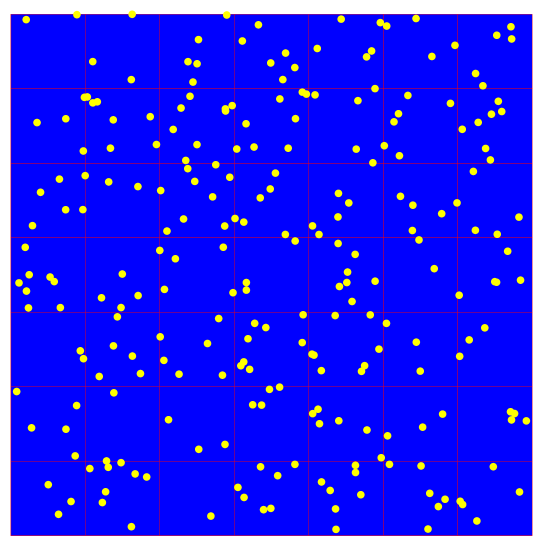
Figure 2: Mosaic of square events representing input for analysis

Such an approach allows us, for example, to exclude regions with a very high or inhomogeneous stellar density. The data sectors of the sky used for analysis are defined in Tab.1.

b$\backslash$l	$\left\langle-5,5\right\rangle$	$\left\langle 85,95\right\rangle$	$\left\langle 175,185\right\rangle$	$\left\langle 265,275\right\rangle$	$\left\langle 45,135\right\rangle$	$\left\langle 225,315\right\rangle$
$\left\langle-5,5\right\rangle$	A	B	C	D	Q2	Q4

b$\backslash$l	$\left\langle 0,360\right\rangle$
$\left\langle-90,-80\right\rangle$	E
$\left\langle 80,90\right\rangle$	F

b$\backslash$l	$\left\langle-45,45\right\rangle$	$\left\langle 45,135\right\rangle$	$\left\langle 135,225\right\rangle$	$\left\langle 225,315\right\rangle$
$\left\langle-60,-45\right\rangle$	Q1S	Q2S	Q3S	Q4S
$\left\langle 45,60\right\rangle$	Q1N	Q2N	Q3N	Q4N

Table 1: MW sectors used for analysis

For analysis we use events defined in Tab.2 and having limited multiplicity

$$M\leq 50.$$ (32)

After this selection, we accept only sources that meet the cut

$$\frac{\Delta v_{gal}}{v_{gal}}\equiv\eta\leq 0.3;\qquad v_{gal}=\left|\mathbf{v}_{gal}\right|.$$ (33)

We have verified that this cut gives almost the same results as a narrower cuts. Most of our calculations focus on mean values, which means that the resulting errors can be much smaller than the errors of individual entries. Thus, unless otherwise stated, we use the cut $\eta$ (33). This ratio can be estimated using (27), (28) and parallax and proper motion errors in the Gaia data as

$$\frac{\Delta v_{gal}}{v_{gal}}\approx\sqrt{\left(\frac{\Delta p}{p}\right)^{2}+\frac{\left(\mu_{l}^{\ast}\Delta\mu_{l}^{\ast}\right)^{2}+\left(\mu_{b}\Delta\mu_{b}\right)^{2}}{\mu^{4}}};\qquad\mu=\sqrt{\mu_{l}^{\ast 2}+\mu_{b}^{2}},$$ (34)

where we have neglected the possible correlation between $p$ and $\mu$. The resulting numbers of sources in the respective sectors are shown in the same table.

	A	B	C	D	E	F	Q2	Q4
$\Delta[\deg]$	0.02	0.02	0.02	0.02	0.04	0.04	0.02	0.02
ncut	332623	1862224	809392	1464150	300037	269708	11561084	10753108

	Q1S	Q2S	Q3S	Q4S	Q1N	Q2N	Q3N	Q4N
$\Delta[\deg]$	0.04	0.04	0.04	0.04	0.04	0.04	0.04	0.04
ncut	1578844	1040017	854355	1378185	1281482	1236598	832720	918059

Table 2: Dimensions of the events and numbers of stars in MW sectors after cuts (32), (33).

III Results

In Fig.3

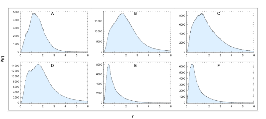
Figure 3: Distribution of distances in the sectors A-F. Unit: r[kpc]. Binning: 0.024kpc.

we show the distribution of star distances in the data sectors A-F defined above. The distance of most of them is $r\lesssim 6-8$ kpc, which is roughly the radius of our analysis. Dependencies of mean velocities $\left\langle v_{l}\right\rangle,\left\langle v_{b}\right\rangle,\left\langle v_{gal}\right\rangle$ and related standard deviations on distance $r$ are shown in the figures that follow. What information can be extracted from them?

III.1 Local velocity of the Sun

The velocity of a star at the point $\mathbf{R}$ of Galactocentric frame can be defined as

$$\mathbf{V}\left(\mathbf{R}\right)=\mathbf{V}_{G}\left(\mathbf{R}\right)+\Delta\mathbf{v}\left(\mathbf{R}\right);\qquad\left\langle\Delta\mathbf{v}\left(\mathbf{R}\right)\right\rangle=\mathbf{0,\qquad V}_{G}\left(\mathbf{R}\right)=\left\langle\mathbf{V}\left(\mathbf{R}\right)\right\rangle,$$ (35)

where $\mathbf{V}_{G}\left(\mathbf{R}\right)$ is the velocity of the galaxy rotation (average velocity at $\mathbf{R}$) and the star local velocity $\Delta\mathbf{v}$ is the deviation from the average $\mathbf{V}_{G}$. Obviously, the average may depend on the choice of sources and the size of the defined neighbourhood. The velocity of the Sun is

$$\mathbf{V}_{\odot}=\mathbf{V}_{G}\left(\mathbf{R}_{\odot}\right)+\mathbf{v}_{\odot};\mathbf{\qquad v}_{\odot}=\left(v_{\odot x},v_{\odot y},v_{\odot z}\right)\equiv\left(U_{\odot},V_{\odot},W_{\odot}\right),$$ (36)

where $\mathbf{v}_{\odot}$ is a local velocity of the Sun and $\mathbf{R}_{\odot}$ its position. The local standard of rest (LSR) is defined as the average $\mathbf{V}_{G}\left(\mathbf{R}_{\odot}\right)$ calculated in the sphere of radius $r\approx 100$pc lsr . The transverse velocity (27) is obtained as the projection of galactic 3D velocity

$$v_{l} =\mathbf{v.n}_{l};\mathbf{\qquad n}_{l}=\left(-\sin l,\cos l,0\right),$$ (37)

$$v_{b} =\mathbf{v.n}_{b};\mathbf{\qquad n}_{b}=\left(-\cos l\sin b,-\sin l\sin b,\cos b\right),$$

where orthonormal vectors $\mathbf{n}_{\alpha}$ represent directions of increasing coordinates $\alpha=l,b$ and the galactic 3D velocity $\mathbf{v}$ is defined as

$$\mathbf{v} =\mathbf{V}\left(\mathbf{R}\right)-\mathbf{V}_{\odot}=\mathbf{V}_{G}\left(\mathbf{R}\right)+\Delta\mathbf{v}\left(\mathbf{R}\right)-\mathbf{V}_{G}\left(\mathbf{R}_{\odot}\right)-\mathbf{v}_{\odot}$$ (38)

$$\left\langle\mathbf{v}\right\rangle =\mathbf{V}_{G}\left(\mathbf{R}_{\odot}\mathbf{+r}\right)-\mathbf{V}_{G}\left(\mathbf{R}_{\odot}\right)-\mathbf{v}_{\odot}.$$ (39)

These equalities allow us a clear interpretation of the panels in Fig.4.

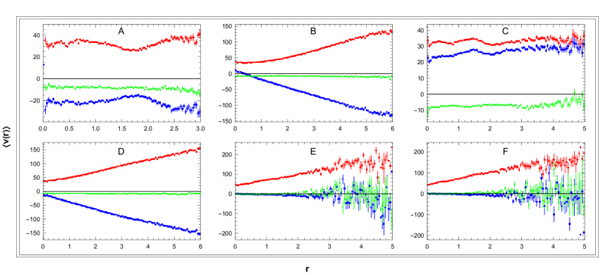
Figure 4: Dependence of  mean velocity ($v_{l}$ - blue, $v_{b}$ - green, $v_{gal}$ - red) on distance $r$ in the galactic reference frame in sectors A-F. Cut $\eta\leq 0.1$. Units: r[kpc], v[km/s].

1) $\left\langle v_{b}\right\rangle$ in the sectors A-D

Since in these sectors we have $b\approx 0$, $z\approx 0,$ so we can identify $v_{z}=v_{b}$. Obviously, the curves $\left\langle v_{b}\right\rangle$ for $r\rightarrow 0$ with the use of (39) define

$$v_{\odot z}=-\left\langle v_{b}\right\rangle.$$ (40)

2) $\left\langle v_{l}\right\rangle$ in the sectors A and C

Similarly, we can identify $v_{y}=+v_{l}$ in the A and $v_{y}=-v_{l}$ in the C sector. Then, for $r\rightarrow 0$ we obtain for A and C

$$v_{\odot y}=-\left\langle v_{l}\right\rangle,\qquad v_{\odot y}=+\left\langle v_{l}\right\rangle.$$ (41)

3) $\left\langle v_{l}\right\rangle$ in the sectors B and D

In these sectors, for small $r$ we can identify $v_{x}=-v_{l}$ in the B and $v_{x}=+v_{l}$ in the D sector. So, for $r\rightarrow 0$ with the use of Eq.(39) we obtain for B and D

$$v_{\odot x}=+\left\langle v_{l}\right\rangle,\qquad v_{\odot x}=-\left\langle v_{l}\right\rangle.$$ (42)

A combined numerical analysis based on the linear fit of the curves $\left\langle v_{l}\right\rangle$ and $\left\langle v_{b}\right\rangle$ for $r\lesssim 1$kpc (Eqs.(40)$-$(42)) gives for $r\rightarrow 0$ the results in Tab.3.

$v_{\odot x}$	$v_{\odot y}$	$v_{\odot z}$	$V_{\odot y}$	ref.
$10.5\pm 1$	$22.5\pm 3$	$7.5\pm 0.5$	$247.5$	this work
$11.1$	$12.24$	$7.25$		sch
	$14.6$		$255.2$	re
$11.1$		$7.8$	$245.8$	ei

Table 3: The local and galactocentric velocities of the Sun [km/s].

III.2 Rotation curve

From now, we will substitute galactic velocity $\mathbf{v}$ in (38) by $\mathbf{v}$ $\rightarrow\mathbf{v}+\mathbf{v}_{\odot}$, so

$$\mathbf{v} =\mathbf{V}_{G}\left(\mathbf{R}\right)+\Delta\mathbf{v}\left(\mathbf{R}\right)-\mathbf{V}_{G}\left(\mathbf{R}_{\odot}\right)$$ (43)

$$\left\langle\mathbf{v}\right\rangle =\mathbf{V}_{G}\left(\mathbf{R}_{\odot}\mathbf{+r}\right)-\mathbf{V}_{G}\left(\mathbf{R}_{\odot}\right)$$ (44)

which does not depend on the velocity of the Sun. The corresponding reference frame is the local rest frame at $\mathbf{R}_{\odot}$. In this frame, the input data (27) are modified with the use of Tab. (3) as

$$v_{l} \rightarrow v_{l}+\mathbf{v}_{\odot}\mathbf{.n}_{l},\qquad v_{b}\rightarrow v_{b}+\mathbf{v}_{\odot}\mathbf{.n}_{b},$$ (45)

$$v_{gal} \rightarrow\sqrt{\left(v_{l}+\mathbf{v}_{\odot}\mathbf{.n}_{l}\right)^{2}+\left(v_{b}+\mathbf{v}_{\odot}\mathbf{.n}_{b}\right)^{2}}.$$ (46)

After this substitution Fig.4 is replaced by panel DATA in Fig.5.

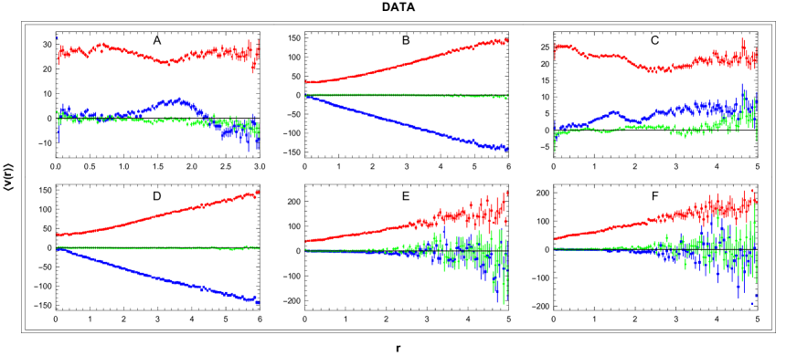
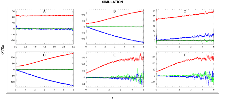
Figure 5: Dependence of  mean velocity ($v_{l}$ - blue, $v_{b}$ - green, $v_{gal}$ - red) on distance $r$ in the local rest frame at $\mathbf{R}_{\odot}$ in sectors A-F. For panel DATA we used cut $\eta\leq 0.1$. Units: r[kpc], v[km/s].

The combination of the new panels A and C, which represents the RC is shown in Fig.6a.

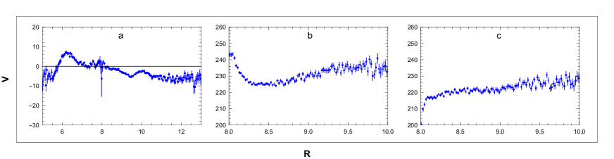
Figure 6: Velocity curves $V=V_{0}(R)-V_{0}(R_{\odot})$ in sectors A+C (panel (a)) and $V=V_{0}(R)$ in sectors B and D (panels (b) and (c)). For panel (a) we used cut $\eta\leq 0.1$. Units: R[kpc], v[km/s].

Another representation of the RC can be obtained from panels B and D. For $\left|Z\right|=0$ and $r>0,$ the term $\mathbf{w}=\mathbf{V}_{G}\left(\mathbf{R}_{\odot}\mathbf{+r}\right)-\mathbf{V}_{G}\left(\mathbf{R}_{\odot}\right)$ in Eq.(44) and its transverse projection $\left\langle w_{l}\right\rangle$ are calculated as suggested in Fig.7 from two similar orthogonal triangles with angle $\alpha.$

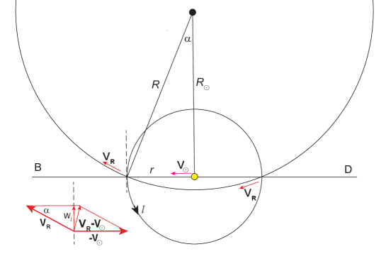
Figure 7: Rotation of MW as seen in sectors B and D. Here the symbols V_R and V_⊙ stand for $\mathbf{V}_{G}\left(\mathbf{R}\right)$ and $\mathbf{V}_{G}\left(\mathbf{R}_{\odot}\right).$

We obtain

$$\left\langle w_{l}\right\rangle=\frac{r}{R}V_{0}\left(R\right);\qquad R=\sqrt{r^{2}+R_{\odot}^{2}}.$$ (47)

Since $w_{l}=-v_{l}$, Eq.(39) implies

$$\left\langle v_{l}\right\rangle =-\frac{r}{R}V_{0}\left(R\right)$$ (48)

$$V_{0}\left(r\right) =-\frac{R}{r}\left\langle v_{l}\right\rangle.$$ (49)

The corresponding RCs are shown in Fig.6b,c. The velocity $V_{0}\left(R\right)$ is roughly constant over the given interval for both panels B and D. This is also confirmed by the numerical analysis of curves in panels B and D in Fig.5 (upper part - data) with the use of (48) and $R_{\odot}\approx 8$ kpc, which gives the result

$$V_{0}\approx 225\,\mathrm{km/s}.$$ (50)

The same value was used in the corresponding simulation shown in the same figure (lower part - simulation). Obviously, the agreement with the data is very good.

III.3 Five parameters of the MW collective rotation

Panels E and F in the upper part of Fig.5 provide further information. We observe $\left\langle v_{l}\right\rangle\approx 0$ and $\left\langle v_{b}\right\rangle\approx 0$, as is expected in both narrow cones pointing perpendicularly from the galactic plane, where positive and negative $v_{l},v_{b}$ are equally abundant. On the other hand the value $\left\langle v_{gal}\right\rangle$ increases with distance from the plane. This increase occurs in the galactic reference frame, which reflects the deceleration of collective rotation in the Galactocentric frame. Important information is obtained from Fig. 8,

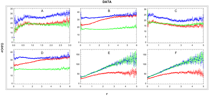
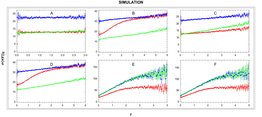
Figure 8: Standard deviations mean velocity ($v_{l}$ - blue, $v_{b}$ - green, $v_{gal}$ - red) on distance $r$ in sectors A-F. Units: r[kpc], $\sigma$[km/s].

where dependencies of standard deviations are shown. The increasing standard deviations in panels E and F suggest a less collective, but more chaotic motion of high velocities away from the galactic plane.

In the distribution (31), we assume in the first approximation:

$$\sigma_{\alpha}=\sigma_{\alpha 0}+\sigma_{\alpha 1}\left|Z\right|;\qquad\alpha=R,\Theta,\Phi,$$ (51)

where $\sigma_{\alpha 0}$ and $\sigma_{\alpha 1}$ are free parameters. In their settings, we proceed as follows.

i) From the data panels A-C in Fig.8 where $Z\approx 0$, we estimate

$$\sigma_{\Theta 0} \approx\sigma_{b}\qquad\text{sectors A-C,}$$ (52)

$$\sigma_{R0} \approx\sigma_{l}\qquad\text{sectors B,D.}$$ (53)

ii) From panels E and F (where $r\approx\left|Z\right|$) we assume the slope

$$\sigma_{\Theta 1}\approx\sigma_{R0}\equiv\sigma_{1},$$ (54)

which implies

$$\sigma_{\Theta}=\sigma_{\Theta 0}+\sigma_{1}\left|Z\right|,\qquad\sigma_{R}=\sigma_{R0}+\sigma_{1}\left|Z\right|.$$ (55)

iii) For distribution $V_{\Phi}$ in (31) we assume different $\sigma_{\Phi}^{\pm}$ for two opposite orientations, $+(-)$ means in (against) the direction of rotation. More specifically:

$$\sigma_{\Phi}^{+}=\sigma_{\Phi 0},\qquad\sigma_{\Phi}^{-}=\sigma_{\Phi 0}+\sigma_{1}\left|Z\right|.$$ (56)

The asymmetry $\sigma_{\Phi}^{\pm}$ reflects an effective deceleration $\left\langle\Delta V_{\Phi}\right\rangle$ of the collective rotation for larger $\left|Z\right|$ mentioned above. We have

$$\left\langle\Delta V_{\Phi}\right\rangle =\frac{1}{N}\left(\int_{-\infty}^{0}V_{\Phi}\exp\left(-\frac{1}{2}\left(\frac{V_{\Phi}}{\sigma_{\Phi}^{-}}\right)^{2}\right)dV_{\Phi}+\int_{0}^{\infty}V_{\Phi}\exp\left(-\frac{1}{2}\left(\frac{V_{\Phi}}{\sigma_{\Phi}^{+}}\right)^{2}\right)dV_{\Phi}\right),$$ (57)

$$N =\int_{-\infty}^{0}\exp\left(-\frac{1}{2}\left(\frac{V_{\Phi}}{\sigma_{\Phi}^{-}}\right)^{2}\right)dV_{\Phi}+\int_{0}^{\infty}\exp\left(-\frac{1}{2}\left(\frac{V_{\Phi}}{\sigma_{\Phi}^{+}}\right)^{2}\right)dV_{\Phi}.$$

After integration we get

$$\left\langle\Delta V_{\Phi}\right\rangle=\sqrt{\frac{2}{\pi}}\left(\sigma_{\Phi}^{+}-\sigma_{\Phi}^{-}\right)=-\sqrt{\frac{2}{\pi}}\sigma_{1}\left|Z\right|.$$ (58)

The free parameters were obtained by optimization to achieve the best fit to the data. At the same time, we have verified  assumptions (55) and (56) provide sufficient freedom to achieve a very good agreement. The list of five empirical parameters used for simulation (31) is given in Tab.4.

$\sigma_{\Theta 0}[km~{}s^{-1}]$	$\sigma_{\Phi 0}[km~{}s^{-1}]$	$\sigma_{R0}[km~{}s^{-1}]$	$\sigma_{1}[km~{}s^{-1}kpc^{-1}]$	$V_{0}[km~{}s^{-1}]$	ref.
$12$	$22$	$30$	$35$	$225$	this work
$11$	$20$	$31$	x	x	vi

Table 4: Parameters of Monte-Carlo simulation and corresponding parameters from other analysis, see Sec. IV.

The comparison with the data is done as follows:

1) Position $\left(r,l,b\right)$ of the star in the galactic reference frame is with the use of Eqs. 1 transformed to the Galactocentric frame $\left(R,\Phi,\Theta\right)$. For this position, the velocity $\mathbf{V}\left(\mathbf{R}\right)$ is generated according to distribution (31) with the parameters from Tab.4. The Wolfram Mathematica code of the generator will be available on the website https://www.fzu.cz/~piska/Catalogue/generator.nb.

2) Simulated transverse velocities $v_{l},v_{b}$ are obtained with the use of (37). Then, the distributions of these velocities can be created in parallel with distributions obtained directly from the data.

In Fig.5 we show the first comparison of data with the Monte-Carlo simulation. For panels B,D,E,F we see a perfect agreement. In panels A and C, the simulation does not reproduce small fluctuations. Simulation in panel C suggests that velocity increases with $r,$ despite the constant parameter $V_{0}$. This small effect is because we are working inside the angle $b=\pm 5$ deg, which means a slight linear increase in average $\left|Z\right|$ and correspondingly some deceleration with $r$. The positive sign of $\left\langle v_{l}(r)\right\rangle_{SIM}$ in sector C is in accordance with the opposite direction of galactic rotation in this sector. So, the corresponding correction should be made to accurately evaluate the RC in these sectors. We have checked that for smaller angles $\left|b\right|$ this effect disappears. At the same time, we do not observe a similar effect in sector A. The reason is that in a very dense field of this sector our cuts $M\leq 50$ and $\eta\leq 0.1$ accept only a narrow sector of the data: $\left|b\right|\lesssim 1~{}$deg.

Relation (48) holds for sectors B and D, where $l\approx\pm\pi/2$ and $Z\approx 0$ (or $b\approx 0$). In general, with the use of (37) and (44) we have

$$\left\langle v_{l}\right\rangle=\left(\mathbf{V}_{G}\left(\mathbf{R}_{\odot}\mathbf{+r}\right)-\mathbf{V}_{G}\left(\mathbf{R}_{\odot}\right)\right)\mathbf{.n}_{l}.$$ (59)

This relation can be rewritten as

$$\left\langle v_{l}\right\rangle=~{}\left(\left(V_{0}+\left\langle\Delta V_{\Phi}\right\rangle\right)\mathbf{N}_{\Phi}\left(\mathbf{R}_{\odot}\mathbf{+r}\right)-V_{0}\mathbf{N}_{\Phi}\left(\mathbf{R}_{\odot}\right)\right)\mathbf{.n}_{l}.$$ (60)

With the use of parameterization (58) and after some calculation, we get

$$V_{0}=\frac{\left\langle v_{l}\right\rangle-\gamma\left\langle\Delta V_{\Phi}\right\rangle}{\gamma-\cos l}=\frac{\left\langle v_{l}\right\rangle+\gamma\sqrt{\frac{2}{\pi}}\sigma_{1}\left|Z\right|}{\gamma-\cos l},$$ (61)

where

$$\gamma=\frac{R_{\odot}\cos l-r\cos b}{\sqrt{R_{\odot}^{2}+r^{2}\cos^{2}b-2R_{\odot}r\cos l\cos b}}$$ (62)

One can check that in sectors B and D this relation reduces to (48). This relation allows us to analyze $V_{0}$ (or $\left\langle\Delta V_{\Phi}\right\rangle$) not only in narrow sectors B and D but also in the wider regions, which can provide higher statistics with smaller errors. In Fig.9

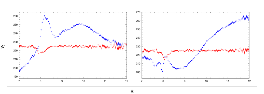
Figure 9: Velocity curves in sectors Q₂ (left) and Q₄ (right): data (blue) and simulation (red). Units: R[kpc], $V_{0}$[km/s].

(blue points) we show RCs obtained with the use of (61) in sectors Q₂ and Q₄. In the analyzed area we observe irregular fluctuations in the rotation velocity $\Delta V_{0}/V_{0}\approx 10\%$. The formula (61) is not suitable for the reconstruction of $V_{0}$ in the region of singularity $\gamma-\cos l\approx 0$ (or equivalently $\mathbf{V}_{G}\left(\mathbf{R}_{\odot}\mathbf{+r}\right)\approx\mathbf{V}_{G}\left(\mathbf{R}_{\odot}\right)$), which takes place for small $r$ or for $\left|\cos l\right|\approx 1$. In the same figure, we show also the curve $V_{0}$ obtained by the reconstruction of Monte-Carlo simulation. The value $V_{0}\approx 225~{}$km/s correctly reproduces the input from Tab.4, which is a check that our calculation is consistent.

The very good agreement of the simulations with the data is confirmed by other results. In Fig.10

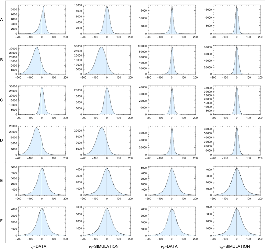
Figure 10: Distributions of $v_{l}$ and $v_{b}$ in sectors A-F: data and simulation. Unit: v[km/s]. Binning: 1.6 km/s.

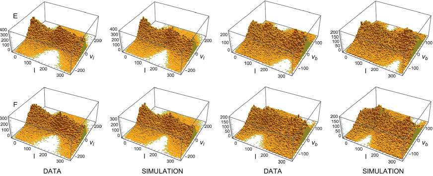
Figure 11: Histograms $\left(v_{l},l\right)$ and $\left(v_{b},l\right)$ in sectors E and F: data and simulation.Units: $l$[deg], $v$[km/s]. Binning $l,v_{l},v_{b}$: $3.6\$deg$,\ 5$ km/s$,\ 3$ km/s.

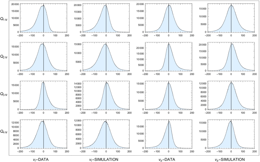
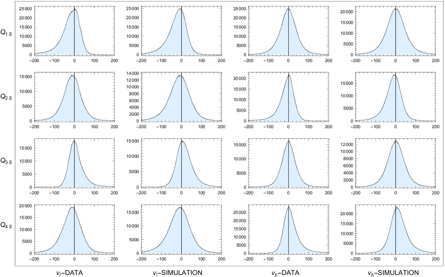
Figure 12: Distributions of $v_{l}$ and $v_{b}$ in sectors Q${}_{1S}-$Q_4S, Q${}_{1N}-$Q_4N: data and simulation. Unit: v[km/s]. Binning: 1.6 km/s.

we show distributions of $v_{l}$ and $v_{b}$ in sectors A-F together with the corresponding distributions obtained from simulations. In sectors A-D we observe a narrower Gaussian distribution of $v_{b}$, the width of which does not depend on the sector. On the other hand, distributions of $v_{l}$ are slightly different. Note the shift in sectors B and D, which corresponds to the decrease in $\left\langle v_{l}\right\rangle$ in upper panels B and D in Fig.5. Next, we see that the agreement between all data and the simulation in Figs.5, 10 is almost perfect. A very good qualitative agreement data - simulation for the standard deviations $\sigma$ of velocity distributions is demonstrated in Fig.8. The important result is shown in Fig.11. The asymmetry of histograms $\left(v_{l},l\right)$ and $\left(v_{b},l\right)$ from sectors E and F with ”cutouts” at $l\approx 0^{\circ},90^{\circ},180^{\circ},270^{\circ}$ reflects different projections of the asymmetry (56). Distributions of velocities in Fig.12 in wide sectors Q${}_{1S}-$Q_4S, Q${}_{1N}-$Q_4N again confirm a very good agreement of the simulation with data.

IV Discussion and conclusion

Our local solar velocity results in Tab.3 are comparable to earlier measurements even though the definition is slightly different. The velocity components $v_{\odot x}$ and $v_{\odot z}$   are in agreement with others, but $v_{\odot y}$ is apparently greater. In our approach, the determination of the local solar velocity $v_{\odot y}$ is not correlated with the velocity $V_{0}$ of MW rotation at the Sun’s position. We also note that our 3D solar velocity vector is obtained only from two components of the proper motion in sectors A-D, without using radial velocity.

The determination of RC is based on the model-independent definition (30). According to this definition, we measure the average value of the collective rotation velocity at the plain of the galactic disc. In Figs.6, 9 we show RCs measured in different regions of galactic longitudes. Its average value well agrees with the results of other measurements listed in Tab.5.

	re	ei	mr	ga1	this work
$V_{0}$	$240\pm 3$	$229\pm 0.2$	$233.6\pm 2.8$	$\approx 230$	$\approx 225$

Table 5: Galactocentric velocity $V_{0}$ [km/s]

Our curves are obtained with very high precision, so as a result, we observe local fluctuations ($\lesssim 30$km/s) in the structure of MW rotation. These fluctuations correspond to velocity substructures and non-axisymmetric kinematic signatures observed in ra ; ga1 . The fluctuations do not allow us to analyze the RC slope in our limited range of $R$ . Further, we have shown that the collective rotation velocity decreases for increasing $\left|Z\right|$, see Eq.(58). A similar observation was reported in wa .

Except for the above local fluctuations, the analyzed kinematical distributions are very well described by a minimal MW model based on five free parameters in the Galactocentric reference frame. The model depicts a simplified scenario where fluctuations in local velocity are smoothed out through averaging. The scale of velocity fluctuations is defined by parameters of the model in Tab.4. It means that their magnitude depends on the direction and increases with distance from the galactic plane. The fluctuations are most significant in the $\mathbf{N}_{R}$ direction, less in the $\mathbf{N_{\Phi}}$ direction and least in the $\mathbf{N_{\Theta}}$ direction.

Analysis and simulation of kinematical distributions in the studied region $\left(r\lesssim 6\mathrm{kpc}\right)$ need apart of the MW parameters also another five parameters related to our laboratory: its velocity $\mathbf{v}_{\odot}$, distance from the galactic centre $R_{\odot}$ and its position $z_{\odot}$ above the galactic plane (neglected). Except for the last two, all the remaining parameters that we obtained in the present analysis are listed in Tabs.3, 4. For now, we ignore the slope of the RC, which has in our region a very small effect ei ; re . The model suggests that the MW rotation can be in the first approximation described as follows.

1) The rotation is strongly collective in the galactic disk plane with relatively small Gaussian velocity fluctuations $\sigma_{\Phi 0},\sigma_{\Theta 0},\sigma_{R0}$ around the much greater velocity $V_{0}$. This is confirmed in Fig.10 in panels $v_{l}$ for sectors A and C, and panels $v_{b}$ for sectors A - D. The broader and slightly shifted distributions $v_{l}$ for sectors B and D are due to the effect of projection illustrated in Fig.7 and expressed in Eq.(48). Our first three parameters are compared with corresponding galactic thin disc parameters obtained in another study, see 4. The agreement is excellent.

2) The fourth parameter $\sigma_{1}$ is important outside the galactic plane, where it controls the increase in fluctuations with $\left|Z\right|$ as shown in sectors E, F in Fig.8. This figure suggests that with increasing $\left|Z\right|$ the collectivity decreases and the directions of the trajectories are becoming more random and probably less circular. An increase of fluctuations suggests also Fig.10 in sectors E,F and Fig.12 in all sectors Q_α, differing from the sectors A-D by $\left|Z\right|>0$. The further effect of $\sigma_{1}$ is due to the asymmetry of distribution $V_{\Phi}$, which generates deceleration of collective rotation with increasing $\left|Z\right|$ according to (58). This asymmetry is manifested very clearly in histograms $\left(v_{l},l\right)$ and $\left(v_{b},l\right)$ in Fig.11. Another representation of the asymmetry in $\left(v_{l},l\right)$ histogram we observe in $v_{l}$ distributions in the sectors Q₁ and Q₃ in Fig.12. Obviously, we have $v_{l}$ $\approx\pm V_{\Phi}$, where the signs $+-$ hold in sectors $1,3$. The asymmetry in $\left(v_{b},l\right)$ histogram is reflected in $v_{b}$ distributions in the sectors Q₂ and Q₄. Our assumption that $\sigma_{\Phi}^{+}$ does not depend on $\left|Z\right|$ is proved by comparing $v_{l}$ distributions in the sectors Q₁ and Q₃ in Fig.12 with the corresponding distributions in sectors A and C in Fig.10. This independence means that

$$\left|\mathbf{V}\left(R,Z\right)\right|\lesssim V_{0}+\sigma_{\Phi}^{+}$$ (63)

in the studied region.

We can conclude that the applied Monte-Carlo model fits the kinematic data in the study area very well. In more distant regions our parameters may require further corrections.

- (1) Bhattacharjee, P., Chaudhury, S., and Kundu, S. 2014, ApJ, 785, 63
- (2) Bland-Hawthorn, J., and Gerhard, O., 2016, Annu. Rev. Astron. Astrophys. 54, 529
- (3) Chen, B., et al. 2001, ApJ, 553, 184
- (4) Eilers, A.-Ch., et al. 2019, ApJ, 871, 120
- (5) Gaia Collaboration (Katz, D., et al.) 2018, A&A, 616, A11
- (6) Gaia Collaboration (Smart, R.L., et al.) 2021, A&A, 649, A6
- (7) Gaia Collaboration (Vallenari, A., et al.) 2023, A&A, 674, A1
- (8) Gaia Data Processing and Analysis Consortium 2023, Gaia Data Release 3, Documentation release 1.2
- (9) Jeans, J.H., 1915, MNRAS, 76, 70
- (10) Kawata, D., et al. 2018, MNRAS Lett., 479, 108
- (11) López-Corredoira, M & Sylos Labini, F., 2019, A&A, 621, A48
- (12) Local standard of rest. (2023, July 25). In Wikipedia. https://en.wikipedia.org/wiki/Local_standard_of_rest
- (13) Mróz, P., et al. 2019, ApJL, 870, 10
- (14) Ramos P., Antoja T., and Figueras F., 2018, A&A, 619, A72
- (15) Reid, M. J., et al. 2014, ApJ, 783, 130
- (16) Schönrich, R., Binney, J., Dehnen, W. 2010, MNRAS, 403, 1829
- (17) Vieira, K., et al. 2022, ApJ, 932, 28
- (18) Wang, H.F., et al. 2023, ApJ, 942, 12
- (19) Zavada P. & Píška K., 2018, A&A, 614, A137
- (20) Zavada P. & Píška K., 2020, AJ, 159,33
- (21) Zavada P. & Píška K., 2022, AJ, 163, 33