Radial Distribution of Distant Trans-Neptunian Objects Points to Sun’s Formation in a Stellar Cluster

Abstract

The Scattered Disk Objects (SDOs) are a population of trans-Neptunian bodies with semimajor axes $50<a\lesssim 1000$ au and perihelion distances $q\gtrsim 30$ au. The detached SDOs with orbits beyond the reach of Neptune (roughly $q>35$ au) are of special interest here as an important constraint on the early evolution of the outer Solar System. The semimajor axis profile of detached SDOs at 50–500 au, as characterized from the Dark Energy Survey (DES), is radially extended, but previous dynamical models of Neptune’s early migration produce a relatively compact profile. This problem is most likely related to Sun’s birth environment in a stellar cluster. We perform new dynamical simulations that account for cluster effects and show that the orbital distribution of SDOs can be explained if a particularly close stellar encounter occurred early on (e.g., M dwarf with the mass $\simeq 0.2$ $M_{\odot}$ approaching the Sun at $\simeq 200$ au). For such an encounter to happen with a reasonably high probability the Sun must have formed in a stellar cluster with $\eta T\gtrsim 10^{4}$ Myr pc^-3, where $\eta$ is the stellar number density and $T$ is the Sun’s residence time in the cluster.

1 Introduction

The dynamical structure of the Kuiper Belt can be used as a clue to the formation and evolution of the Solar System, planetary systems in general, and Neptune’s early orbital history in particular. The exact nature of Neptune’s orbital migration has been the subject of considerable research (see Morbidelli & Nesvorný 2020 and Gladman & Volk 2021 for recent reviews). The problem is best addressed by forward modeling where different initial conditions and Neptune’s orbital evolutions are tested, and the model predictions are compared to observations. Initial studies envisioned dynamical models where Neptune maintained a very low orbital eccentricity, comparable to the present $e_{\rm N}\simeq 0.01$, during its early migration (e.g., Malhotra 1993, 1995; Gomes 2003; Hahn & Malhotra 2005). A giant-planet instability model was later proposed to explain the somewhat excited orbits of the outer planets (Tsiganis et al. 2005). In the original instability model, Neptune was scattered to a highly eccentric orbit ($e_{\rm N}\gtrsim 0.2$) that briefly overlapped with the Kuiper Belt (Levison et al. 2008).

Different arguments have been advanced to rule out specific migration/instability regimes (e.g., Batygin et al. 2011; Dawson & Murray-Clay 2012). For example, the high-eccentricity instability model with rapid (e-fold $\tau\sim 1$ Myr) circularization of Neptune’s orbit does not reproduce the wide inclination distribution of Kuiper belt objects (KBOs), because there is not enough time to dynamically excite orbits in this model (Volk & Malhotra 2011, Nesvorný 2015a). The migration models with a very low eccentricity of Neptune ($e_{\rm N}\lesssim 0.03$; Volk & Malhotra 2019) do not explain KBOs with $50<a<60$ au, perihelion distances $q>35$ au, and $i<10^{\circ}$ (Nesvorný 2021). Most modern studies therefore considered a mild version of the instability with $e_{\rm N}\simeq 0.03$–0.1 and $\tau\sim 10$ Myr (Nesvorný & Morbidelli 2012; Kaib & Sheppard 2016; Deienno et al. 2017, 2018; Lawler et al. 2019; Clement et al. 2021).

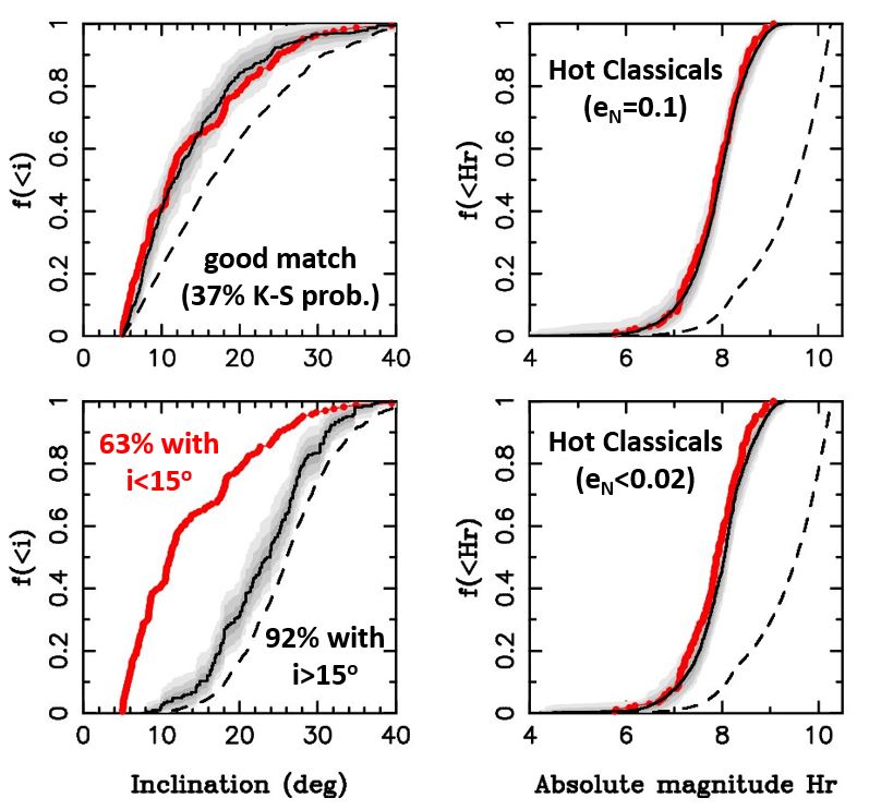
Figure 1: A comparison between the biased model (black lines) and OSSOS observations (red dots) of Hot Classicals ($40<a<47$ au, $q>36$ au, $i>5^{\circ}$; Nesvorný et al. 2020). The intrinsic model distributions are shown as dashed lines. The shaded areas are 1$\sigma$ (bold gray), 2$\sigma$ (medium) and 3$\sigma$ (light gray) envelopes. We used the model results and generated 10,000 random samples with 164 bodies each (the sample size identical to the number of OSSOS detections). The samples were biased with the OSSOS simulator (Lawler et al. 2018). We identified envelopes containing 68.3% (1$\sigma$), 95.5% (2$\sigma$) and 99.7% (3$\sigma$) of samples and plotted them here. The bottom panels show a model with the low-eccentricity migration of Neptune ($e_{\rm N}\simeq 0.01$). In this case, orbits are decoupled from Neptune by the Kozai resonance (Kozai 1962) and this creates a specific inclination distribution with very few orbits below $15^{\circ}$ (Nesvorný 2021). The upper panels show a successful model where Neptune’s eccentricity was excited to $e_{\rm N}=0.1$ when Neptune reached $\simeq 28$ au, and slowly damped afterwards. The K-S test applied to the inclination distributions from the successful and unsuccessful cases gives 37% and $<10^{-10}$ probabilities, respectively, that the (biased) model and observed distributions are drawn from the same underlying distribution. Figure adapted from Nesvorný et al. (2020).

In the previous work, we developed dynamical models for resonant and dynamically hot KBOs (Nesvorný & Vokrouhlický 2016), dynamically cold KBOs (Nesvorný 2015b) and SDOs (Kaib & Sheppard 2016, Nesvorný et al. 2016). The newest of these models were constrained by the Outer Solar System Origins Survey (OSSOS; Bannister et al. 2018) observations (Nesvorný et al. 2020). For example, Fig. 1 compares a successful dynamical simulation with a model where Neptune was assumed to have migrated on a low-eccentricity orbit ($e_{\rm N}\simeq 0.01$). The results indicate that Neptune’s migration was long-range (from $\lesssim 25$ au to 30 au), slow ($\tau\gtrsim 10$ Myr) and grainy (due to scattering encounters with Pluto-sized objects), and that Neptune’s eccentricity was excited to $e_{\rm N}\simeq 0.03$–0.1 when Neptune reached $\simeq 28$ au (probably due to an encounter with a planetary-class object).

Here we consider SDOs. SDOs can be divided into scattering and detached populations. Gladman et al. (2008) defined scattering SDOs as objects that are dynamically coupled to Neptune (semimajor axis change $\Delta a>1.5$ au in a 10-Myr long integration window, plus $a>47.8$ au), and detached SDOs as those that are not coupled (non-resonant, $\Delta a<1.5$ au, and $e>0.24$ to avoid classical KBOs). Here we adopt a simpler definition. We avoid orbits with $a<60$ au because we do not want to mix arguments about the formation of distant/detached SDOs with those related to capture of bodies into the strong 5:2 resonance at $a\simeq 55.5$ au (Gladman et al. 2012). The objects with $60<a<500$ au are separated to those with the perihelion distance $q=a(1-e)<35$ au (our scattering SDOs) and $q>35$ au (our detached SDOs). There is a good overlap with the definition of Gladman et al. (2008) because SDOs with $q<35$ au are typically scattered by Neptune while the ones with $q>35$ au are not. Importantly, we apply the same (our) definition to both the model and observed populations – this allows us to accurately compare the two.

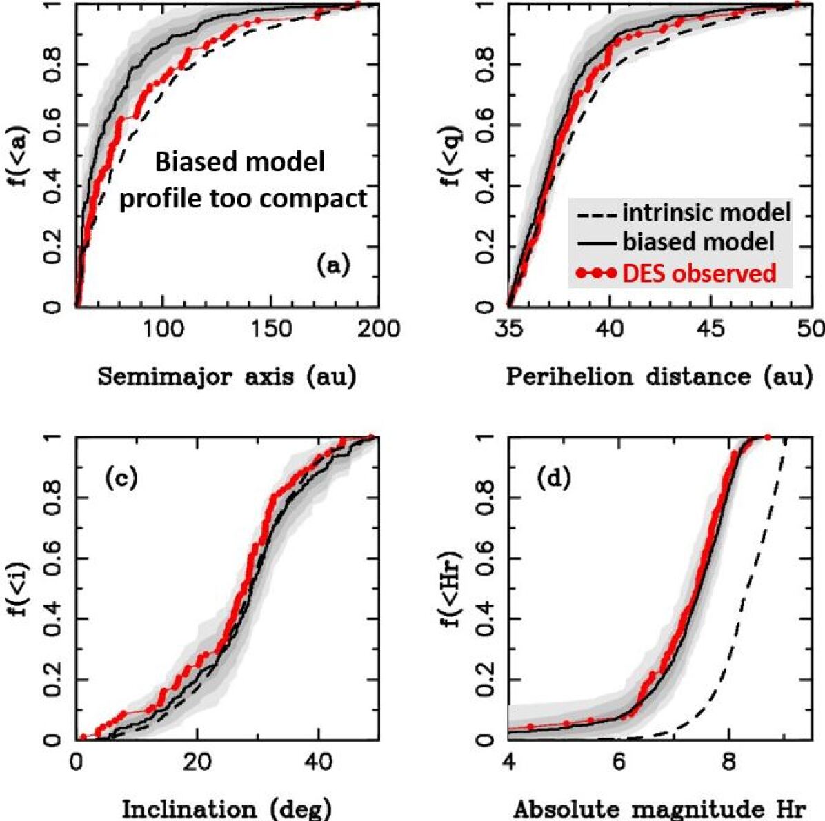
Figure 2: The problem with detached SDOs. The plot shows a comparison between the biased model (black line) from our Galaxy simulation and Dark Energy Survey (DES) observations (red lines) of detached SDOs. See Sect. 2 for the description of model parameters and DES (Bernardinelli et al. 2022). The intrinsic model distributions are shown as dashed lines. See the caption of Fig. 1 for the meaning of shaded areas. The Kolmogorov-Smirnov (K-S) test applied to the semimajor axis distribution (panel a) gives only a 1.3% probability that the biased model and observed distributions are drawn from the same underlying distribution.

Our immediate objective in this work is to resolve a longstanding problem with detached SDOs. The problem is illustrated in Fig. 2, where the biased model shows a radial profile with far fewer detached SDOs at larger orbital radii than observations. Something is clearly off here. The radial profile problem exists for all migration models that we tested so far. Specifically, we tested models with: (1) different timescales of Neptune’s migration ($\tau=5$, 10, 30 and 100 Myr), (2) different excitation of Neptune’s eccentricity (e.g., $e_{\rm N}=0$, 0.03 and 0.1), (3) different damping timescales of Neptune’s eccentricity (e-fold $\tau_{e}=5$, 10, 30 and 100 Myr), (4) different radial profiles of the original planetesimal disk (Nesvorný et al. 2020), and (5) with and without Neptune’s jump during the instability. The problem persists independently of whether the galactic potential/stars are included in the model (Nesvorný et al. 2017). Moreover, while the problem was originally identified when the model was compared with the Outer Solar System Origins Survey (OSSOS) detections, it is even more evident in the comparison with the Dark Energy Survey (DES) observations of SDOs (Bernardinelli et al. 2022) (Fig. 2).

We now believe to have found an interesting solution to this problem. To test it, we performed new simulations with a stellar cluster (Adams 2010). The cluster potential and encounters with cluster stars were modeled following the methods described in Batygin et al. (2020) (Sect. 2). In all other aspects the dynamical model remained the same. As we discuss in Sect. 3, the new model produced the same orbital distribution of KBOs for $a<50$ au. For $a>50$ au, however, the model population of detached SDOs is more radially extended when the cluster effects are accounted for. Moreover, when we assume that a particularly close stellar encounter occurred early on, the model is able to accurately match the radial profile of detached SDOs detected by DES (Bernardinelli et al. 2022; Sect. 3).

The stellar cluster effects were previously invoked to explain extreme KBOs (Kenyon & Bromley 2004; Morbidelli & Levison 2004; Brasser et al. 2006, 2012; Brasser & Schwamb 2015), such as (90377) Sedna and 2012 VP113 ($a>200$ au, $q\simeq 75$–80 au; Brown et al. 2004, Trujillo & Sheppard 2014). The results indicate that the Sun was born in a cluster with $N\sim 10^{3}$ or more stars, and that the Sun remained in the cluster for at least $T\sim 10$ Myr. With only a few extreme KBOs known, however, these results are subject to small number statistics. In addition, the extreme KBOs were detected in different observational programs that employed different search strategies and had different limiting magnitudes. It is therefore not obvious how to model the strong biases involved in their detection. That is why the radial structure of detached SDOs with $35<q<50$ au, which is well characterized from DES observations ($\simeq 200$ detected KBOs with $a>50$ au), can represent a useful constraint on cluster properties.

2 Methods

Migration model. The numerical integrations consist of tracking the orbits of the four giant planets (Jupiter to Neptune) and a large number of planetesimals. Uranus and Neptune are initially placed inside of their current orbits and are migrated outward. The swift_rmvs4 code, part of the Swift $N$-body integration package (Levison & Duncan 1994), is used to follow all orbits. The code was modified to include artificial forces that mimic the radial migration and damping of planetary orbits. The migration histories of planets are informed by our best models of planetary migration/instability. Specifically, we adopt the migration model s10/30j from Nesvorný et al. (2020) that worked well to satisfy various constraints; see that work for a detailed description of the migration parameters (e.g., $\tau=10$ Myr for $t<10$ Myr and instability at $t=10$ Myr). The code accounts for the jitter that Neptune’s orbit experiences due to close encounters with very massive bodies (Nesvorný & Vokrouhlický 2016).

Planetesimal Disk. Each simulations includes one million disk planetesimals distributed from 4 au to beyond 30 au. Such a high resolution is needed to obtain good statistics for SDOs. We tested different initial disk profiles that produced the best fits to the classical Kuiper Belt in Nesvorný et al. (2020). For the truncated power-law profile (Gomes et al. 2004), the step in the surface density at 30 au is parameterized by the contrast parameter $c\sim 10^{3}$, which is simply the ratio of surface densities on either side of 30 au. The exponential disk profile is parameterized by one e-fold $\Delta r\sim 2.5$ au (Nesvorný et al. 2020). The initial eccentricities and inclinations of orbits are set according to the Rayleigh distribution. The disk bodies are assumed to be massless such that their gravity does not interfere with the migration/damping routines.

Cluster potential and cluster star encounters. The gravitational potential of a cluster (stars and gas) is modeled by the Plummer model (Plummer 1915). Adopting the mean stellar mass of $\langle M_{*}\rangle=0.38$ $M_{\odot}$ (Kroupa 2001), for the reference cluster mass $M=1200$ $M_{\odot}$ (roughly comparable to the Orion Nebular Cluster) and the Plummer radius $r_{\rm P}=0.35$ pc, the average and central stellar number densities are $\eta=100$ pc^-3 and $\eta_{\rm c}=1.7\times 10^{4}$ pc^-3, respectively (Hillenbrand & Hartmann 1998). We perform two simulations for clusters with $N=1000$ stars and the Sun’s residence time in the cluster $T=10$ Myr (time measured after the gas disk dispersal; $t=0$ in our simulations) that differ in the history of stellar encounters with the Sun. [For brevity, we sometimes refer to $T$ as the “cluster lifetime”, but see the discussion below.] In the first case, we opt to model a case where all stellar encounters were relatively distant ($r\gtrsim 1000$ au; hereafter the Cluster1 simulation). In the second case, we model close stellar encounters (Fig. 3; Cluster2). For reference, we also run an additional case without the star cluster (Galaxy). The Sun has a orbit near the reference radius $\sqrt{2/3}\,r_{\rm P}$.

Before advancing our discussion, it is imperative to clarify the limitations of the cluster model we have adopted. Although the chosen parameters are roughly comparable to the characteristics of the Orion Nebula Cluster (ONC), the Plummer model is, by nature, an oversimplification. In a more precise rendition of stellar dynamics, the Sun would not maintain a static orbit around the cluster core but would instead execute a complex and chaotic trajectory. Furthermore, star clusters themselves evolve, with both the gas density and the stellar number density diminishing in time. Detailed modeling of these effects would introduce an element of time-dependence into our picture that we currently disregard. Nevertheless, we do not expect that these assumptions pose a significant limitation for our work, because, as we demonstrate below, our results depend most strongly on the time-integrated stellar number density in the Sun’s vicinity, not the instantaneous value of $\eta$ itself. Consequently, our model can be seen as a means to replace a stochastic integrand with a representative average value.

It is also worth highlighting that the quoted cluster lifetime $T$ should not be mistaken for the actual longevity of the star cluster. It would be more accurate to interpret this period as representing the Sun’s duration of residence within its birth association (the ONC itself is likely to progress into an open cluster over time, possibly bearing resemblance to the loosely-bound Pleiades cluster in roughly 100 Myr; Kroupa 2001). Consequently, while our model does not fully capture the intricacies of star cluster dynamics, it should provide us with a reliable means to investigate the effects of the solar system’s birth environment on the trans-Neptunian region. Additional constraints on the solar system’s birth environment are discussed in Section 5.

The effect of stellar encounters is modeled in swift_rmvs4 by adding a star at the beginning of its encounter with the Sun and removing it after the encounter is over. The stars are released and removed at the heliocentric distance of 0.1 pc (20,600 au; increasing this value does not appreciably change the results). We use the model of Heisler et al. (1987) to generate stellar encounters but omit white dwarfs to approximate the Initial Mass Function (IMF, Kroupa 2001). In contrast to Heisler et al. (1987), we assume a common velocity dispersion $\langle v\rangle\sim 1$ km s^-1 and draw velocities from the Maxwell–Boltzmann distribution with a scale parameter $\sqrt{2}\langle v\rangle$ (Binney & Tremaine 1987). This choice is motivated by observational surveys of clusters (Lada & Lada 2003).

Galactic potential and stellar encounters. Effects of the Galaxy become important after the Sun leaves the cluster. We assume that the Galaxy is axisymmetric and the Sun follows a circular orbit in the Galactic midplane (Sun’s migration in the Galaxy is not included; Kaib et al. 2011). The Galactic tidal acceleration is taken from Levison et al. (2001) (see also Heisler & Tremaine 1986, Wiegert & Tremaine 1999). The mass density in the solar neighborhood is set to $\rho_{0}=0.15$ $M_{\odot}$ pc^-3. The stellar mass and number density of different stellar species are computed from Heisler et al. (1987). The stars are released and removed at the heliocentric distance of 1 pc (206,000 au). For each species, the velocity distribution is approximated by the isotropic Maxwell–Boltzmann distribution. The dynamical effect of passing molecular clouds is ignored.

Comparison with observations. We compare the model results with DES detections of SDOs. DES covered a contiguous 5000 $\deg^{2}$ of the southern sky between 2013-2019, with the majority of the imaged area being at high ecliptic latitudes. The search for outer Solar System objects yielded 812 KBOs with well-characterized discovery biases, including over 200 SDOs with $a>50$ au. The DES observations are more constraining in this work than OSSOS given that DES detected more SDOs, as expected from the differences in the geometry of both surveys. The DES survey simulator (Bernardinelli et al. 2022) enables comparisons between population models and the DES data by simulating the discoverability conditions of each member of the test population, that is, the model is biased in the same way as the data. These simulations enable the application of standard statistical tests (e.g., Kolmogorov–Smirnov) to establish whether a tested model can be ruled out from DES observations.

Absolute magnitude distribution. After experimenting with different magnitude distributions, we found a setup that works pretty well (Sect. 3). The size distribution is assumed to be a broken power law with the knee $D_{\rm knee}=100$ km and the ankle $D_{\rm ankle}=300$ km. The size distribution of small bodies with $D<D_{\rm knee}$ is approximated by the cumulative power law $N(D)\propto D^{-q_{\rm small}}$ with $q_{\rm small}=2.1$ (Nesvorný 2018). The distant KBOs below some minimum size are not detected by DES. For detached SDOs with $60<a<500$ au, we set the minimum diameter $D_{\rm min}=70$ km ($D_{\rm min}=40$ km is used for Hot Classicals). The intermediate size bodies with $D_{\rm knee}<D<D_{\rm ankle}$ are given $q_{\rm inter}=4.5$ and the large bodies with $D>D_{\rm ankle}$ are given $q_{\rm inter}=2.0$. We used the albedo $p_{\rm V}=0.05$ to convert diameters to the absolute (visual) magnitudes ($H$). As the DES detections are reported in the red filter, we use the red magnitude $H_{\rm r}=H-0.6$. The DES selection function (weakly) depends on the color of each object, so we applied the color transformations from Section 2.3 of Bernardinelli et al. (2022) to each object. We also assumed that the objects have no variability (i.e. a flat or constant light curve).

3 Results

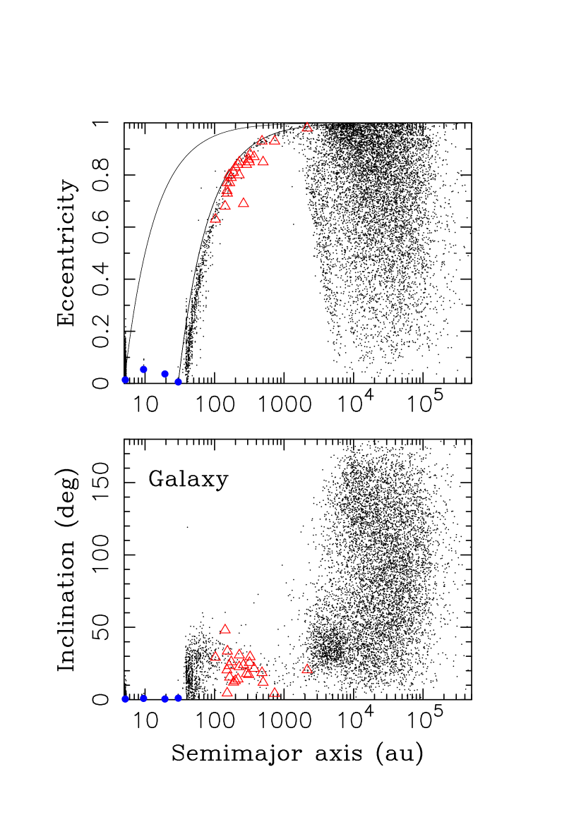
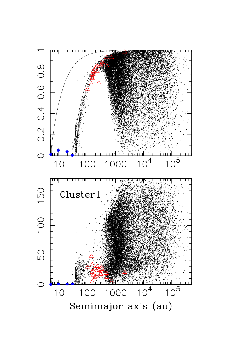
Figure 4: The orbital distribution of bodies from three models: (1) no cluster (labeled Galaxy), (2) a cluster with relatively distant stellar encounters (Cluster1), and (3) a cluster with relatively close stellar encounters (Cluster2). All simulations included the galactic tide and encounters of the Sun with stars in the Galaxy. We sub-sampled the model population, shown here at the simulated time $t=4.6$ Gyr (present epoch), by a factor of four to limit saturation. The red triangles show orbits of known extreme KBOs.

We propose that the problem with the radially extended distribution of detached SDOs (Fig. 2 and discussion in Section 1) can be resolved when it is accounted for the effects of close stellar encounters during the solar system’s cluster stage. To introduce this possibility, we first discuss the results of our three simulations – Galaxy, Cluster1 and Cluster2 – and point out major differences between them. The orbital distributions of bodies obtained in our three models are similar for $a<50$ au and $a>10$,000 au but show important differences for $50<a<10$,000 au (Fig. 4). With the cluster star encounters in Cluster1 and Cluster2, bodies with $50<a<10$,000 au can decouple from Neptune and evolve onto orbits with lower eccentricities and large inclinations. This creates a spherical cloud of bodies with the overall structure similar to the Oort cloud (Oort 1950) but located at smaller orbital radii. We call this the Fernández cloud (Fernández 1997). See Fernández (1997), Fernández & Brunini (2000), Morbidelli & Levison 2004, Brasser et al. (2006, 2012) and Kaib & Quinn (2008) for previous studies.

The boundary between the Oort and Fernández clouds is not well defined. Comparing different panels in Fig. 4, we find that nearly all Oort cloud objects have $a>2$,000 au and the great majority have $a>5$,000 au. In our cluster models, the Fernández cloud forms at $a<5$,000 au and extends inwards to $a\simeq 200$–300 au. To fix the terminology in this work, the bodies with $250<a<5$,000 are called the Fernández cloud objects (FCOs) and the bodies with $a>5$,000 au are Oort cloud objects (OCOs). We note that the Oort cloud can divided into two parts: the (active) outer part with $a\gtrsim 15$,000 au (Hills 1981, Duncan et al. 1987, Vokrouhlický et al. 2019), which the source of most long-period comets, and the (inactive) inner part with $a\lesssim 15$,000 au, where most orbits remain unchanged (except when very close stellar encounters happen). The outer Oort cloud extends to $a\gtrsim 10^{5}$ au.

Without the stellar cluster, we find that $\simeq 3$% of bodies originally from 4–30 au end up in the Oort cloud (Table 1). This fraction does not change when we account for the cluster. This means that the stellar cluster environment does not strongly influence the population of OCOs, at least for the migration and stellar cluster parameters adopted in this work (Sect. 2, $\tau\sim T$; see Sect. 4 for further discussion). With the stellar cluster, roughly 7% of bodies from 4–30 au end up in the Fernández cloud.

The implantation probabilities given in Table 1 would have to be multiplied by the number of planetesimals originally available in each source zone to obtain the population estimates for different target zones. For example, for the reference surface density profile, $\Sigma\propto 1/r$, there is an equal number of bodies in each semimajor axis interval. In this case, the inner SDOs ($50<a<250$ au) and OCOs would predominantly originate from planetesimals in the 20–30 au zone, and the Fernández cloud – for the Cluster1 and Cluster2 models – would be a mix of planetesimals from every zone (implantation probabilities: 6.8–7.2% from the Jupiter/Saturn zone at 4–10 au, 7.6–8.1% from the Uranus/Neptune zone at 10–20 au, and 6.3–6.8% from the outer disk at 20–30 au).

It is expected that the planetesimal populations in the Jupiter/Saturn and Uranus/Neptune zones become depleted by the end of the gas disk lifetime ($t=0$ in our simulations). These planetesimals are scattered inward and outward by the growing giant planets and their orbits can be circularized by the gas drag. They can end up the asteroid belt or in the outer disk at $>20$ au (Kretke et al. 2012, Raymond & Izidoro 2018, Vokrouhlický & Nesvorný 2019). If so, the fractions reported for the outer disk – the last column in Table 1 – could be the most relevant.

For $\simeq 20$ $M_{\rm Earth}$ of planetesimals between 20 and 30 au (Nesvorný 2018), the Fernández and Oort clouds would end up having $\simeq 1.3$ $M_{\rm Earth}$ and $\simeq 1$ $M_{\rm Earth}$, respectively (for Cluster2; the estimates for Cluster1 are similar). With $(8\pm 3)\times 10^{9}$ planetesimals in the outer disk with diameters $D>10$ km (Nesvorný et al. 2019), the Fernández and Oort clouds would end up having $(5\pm 2)\times 10^{8}$ and $(4\pm 2)\times 10^{8}$ $D>10$ km bodies today. The inner SDOs at 50–250 au should represent a much smaller population with estimated (2.4–$4)\times 10^{7}$ $D>10$ km bodies today.

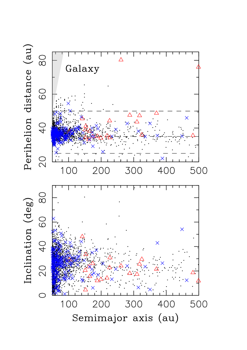
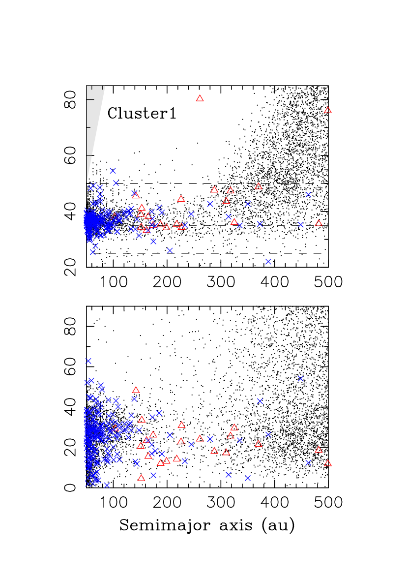
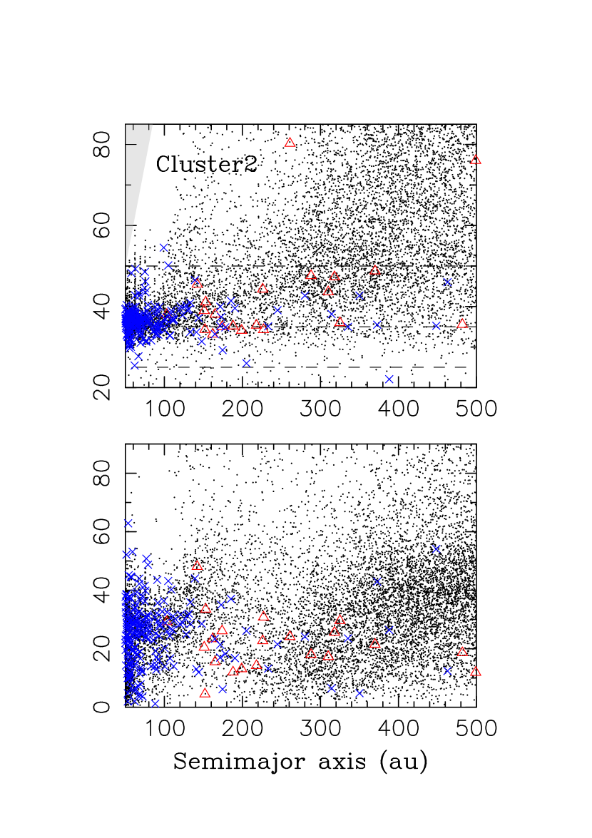
Figure 5: The orbital distribution of bodies from three models: (1) no cluster (labeled Galaxy), (2) a cluster with relatively distant stellar encounters (Cluster1), and (c) a cluster with relatively close stellar encounters (Cluster2). All simulations included the galactic tide and encounters of the Sun with stars in the Galaxy. The model population are shown here at the simulated time $t=4.6$ Gyr (present epoch). The red triangles show orbits of known extreme KBOs. The blue crosses are DES detections (Bernardinelli et al. 2022).

Figure 5 shows the orbital distribution for $60<a<500$ au in more detail. The figure highlights the relationship between SDOs and FCOs. In the Galaxy simulation, the detached SDOs with $q>35$ au are dropouts from the orbital resonances with Neptune (Kaib & Sheppard 2016, Lawler et al. 2019). While most dropout SDOs have $35<a<50$ au, some with $a\lesssim 150$ au can have higher perihelion distances (as high as $q\simeq 60$ au). In the Cluster1 and Cluster2 models, FCOs form during close encounters of the cluster stars. Most FCOs have orbits with $a>200$ au and $q>50$ au and can be clearly distinguished from the dropout SDOs. But there is also a large population of FCOs with $a<200$ au and $35<q<50$ au, especially in the Cluster2 model, where bodies would be formally classified as detached SDOs. This shows how the orbital structure of detached SDOs changes when the cluster effects are taken into account. Specifically, the radial profile of detached SDOs is more extended in the cluster simulations than without a cluster (Fig. 6). This works in the right direction to resolve the problem that motivated this work (Sect. 1).

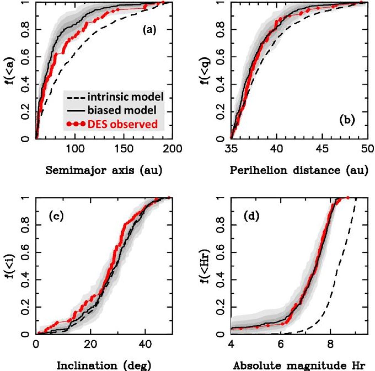
Figure 7: A comparison between the biased model (black line) from the Cluster1 simulation and DES observations (red lines) of detached SDOs. The intrinsic model distribution is shown as a dashed line. See the caption of Fig. 1 for the meaning of shaded areas. The K-S test applied to the semimajor axis distribution (panel a) gives only a 2.9% probability that the biased model and observed distributions are drawn from the same underlying distribution.

Our Galaxy simulation (i.e., no cluster) was unsuccessful in reproducing the radial structure of detached SDOs observed by DES (Fig. 2). We applied the Kolmogorov-Smirnov (K-S) test to find that the semimajor axis distribution of detached SDOs obtained in this model – based on the comparison of with DES observations – can be rejected with a 98.7% probability. Small changes of the input size distribution do not significantly influence this result. The comparison is done for $60<a<200$ au and $35<q<50$ au because this is where the DES observations are the most diagnostic (e.g., only one detached SDO detected by DES with $q>50$ au). The extended range $60<a<500$ au is tested below. The radial distribution of detached SDOs obtained in the Cluster1 model shows a similar problem (Fig. 7). Again, the biased model shows a more compact profile than the DES observations. The K-S test applied to the semimajor axis distribution (panel a in Fig. 7) suggest that that the model can be rejected with a 97.1% probability.

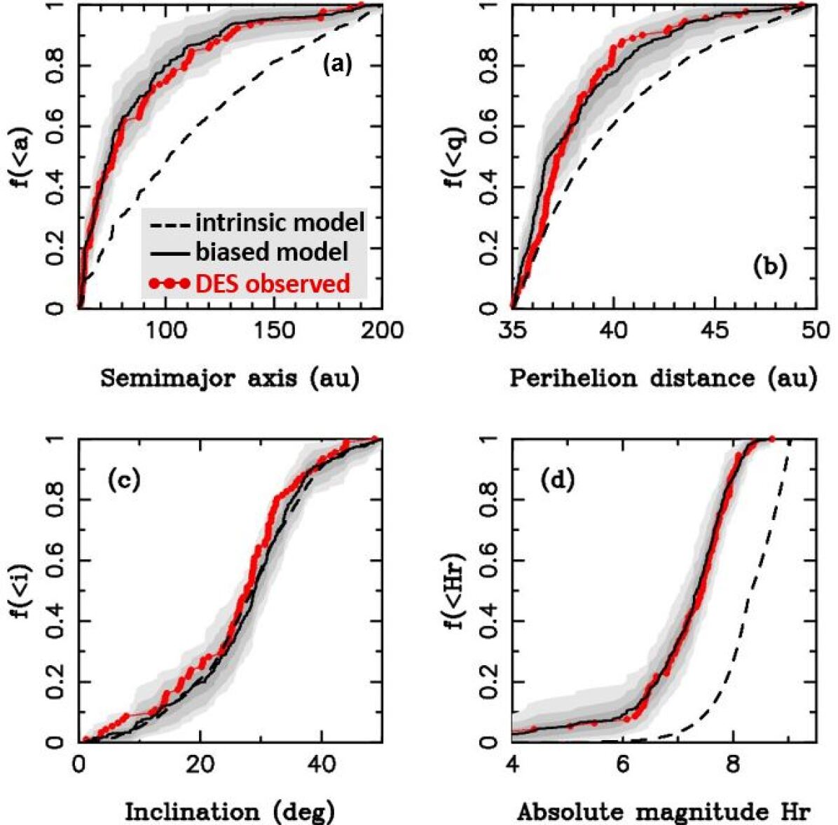
Figure 8: A comparison between the biased model (black line) from the Cluster2 simulation and DES observations (red lines) of detached SDOs. The intrinsic model distribution is shown as a dashed line. See the caption of Fig. 1 for the meaning of shaded areas. DES detected 92 detached SDOs in the range shown here.

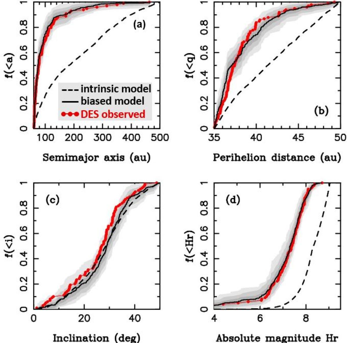
Figure 9: The same as Fig. 8 but now for the extended semimajor axis range $60<a<500$ au. See the caption of Fig. 1 for the meaning of lines, symbols and shaded areas. DES detected 99 detached SDOs in the range shown here.

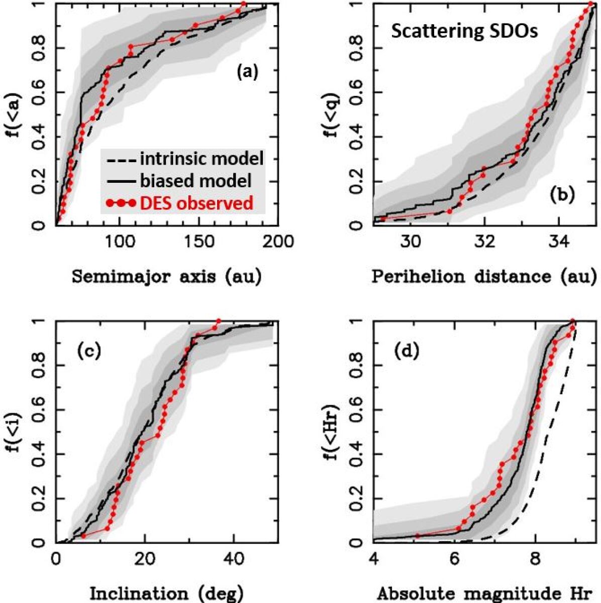
Figure 10: A comparison between the biased model (black line) from the Cluster2 simulation and DES observations (red lines) of scattering SDOs. The intrinsic model distribution is shown as a dashed line. See the caption of Fig. 1 for the meaning of shaded areas. The statistics for the scattering SDOs shown here is as not as good as the one shown for the detached SDOs in Fig. 8, because DES detected only 31 scattering SDOs in the range shown here.

Finally, in the Cluster2 model with a very close stellar encounter (0.17 $M_{\odot}$ star at distance $d\simeq 175$ au), the match to DES observations is good (Fig. 8). The population of detached SDOs is radially extended as it should be, the perihelion and inclination distributions look great as well. The K-S test applied to the semimajor axis distribution gives a 84% probability that the two distributions are statistically the same. The agreement in the extended semimajor axis range is equally good (Fig. 9; 82% K-S test probability). For completeness, we also show a comparison between the Cluster2 model and DES observations for the scattering disk (Fig. 10). As we explained in Sect. 1, the scattering disk population is particularly easy to model because its current orbital structure is practically independent of the dynamical evolution of the early Solar System.

For Cluster2, our results suggest that there should be a transition in the orbital structure of trans-Neptunian objects (TNOs) near 100 au. For $a\lesssim 100$ au, most TNOs should be dropouts from resonances with migrating Neptune (Kaib & Sheppard 2016, Nesvorný et al. 2016). The detached SDOs with $a\lesssim 100$ au should thus concentrate near orbital resonances (e.g., 3:1, 4:1, 5:1; Lawler et al. 2019). The resonant dropouts have moderate perihelion distances and moderate inclinations ($q\lesssim 60$ au, $i\lesssim 50^{\circ}$). The orbital structure should change for $a>100$ au, where most TNOs should have decoupled from Neptune during the cluster stage (see Cluster2 in Fig. 5). These FCOs can have large perihelion distances and large inclinations, and their number should increase with the semimajor axis (the FCO population at 250–5000 au can represent several Earth masses). We do not find any diagnostic correlations between different orbital parameters. There is a slight enhancement of FCO inclinations near 40^∘, which is probably related to the geometry of the closest encounter in our Cluster2 simulation. In Cluster1, there is a slight enhancement for $i\simeq 30^{\circ}$.

4 Constraints from Cold Classicals

Above we showed that a close stellar encounter, e.g., 0.17 $M_{\odot}$ star at distance $d\simeq~{}175$ au, could have affected the radial profile of detached SDOs. Here we ask whether such a close encounter would be compatible with the inclination distribution of Cold Classicals (CCs). CCs are population of KBOs with orbits $42<a<47$ au, $q>36$ au and $i<5^{\circ}$ (Gladman et al. 2008). They are thought to have formed in situ and remained largely undisturbed during Neptune’s migration (Batygin et al. 2011, Dawson & Murray-Clay 2012).

Batygin et al. (2020) highlighted the importance of the inclination distribution of CCs as an important constraint on stellar encounters. The inclination distribution of CCs is well described by a Rayleigh distribution with a scale parameter $\sigma_{i}=1.7$ deg (mean inclination $\langle i\rangle=\sqrt{\pi/2}\,\sigma_{i}=2.1$ deg). Batygin et al. (2020) showed that the low orbital inclinations of CCs can be used to set an upper limit on $\eta T$, because very close stellar encounters could happen for large values of $\eta T$, and these encounters would excessively excite inclinations.

The fraction of cluster realizations that are incompatible with the the inclination distribution of CCs increases with $\eta T$. For example, clusters with $\eta T>3\times 10^{4}$ Myr pc^-3 have a $\gtrsim 50$% probability to be incompatible (Sect. 5.2 in Batygin et al. 2020). For $\eta T\sim 10^{4}$ Myr pc^-3, which is the reference cluster tested here, the probability of being incompatible is only $\sim 20$%. We therefore see that the cluster parameters adopted in this work are consistent with low orbital inclinations of CCs.

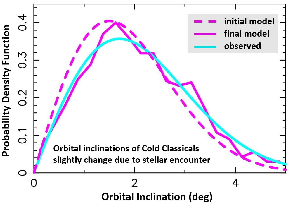
Figure 11: The observed inclination distribution of CCs (blue line) is compared to model results (purple lines). We distributed 1,000 test CCs on initial orbits with $42<a<47$ au and $q>36$ au. The initial inclinations followed a Rayleigh distribution with $\sigma_{i}=1.5$ deg (dashed line). The orbits were integrated for 10 Myr in the Cluster2 model, including the close stellar encounter at $t\simeq 5.17$ Myr (Fig. 3). The inclination distribution did not change much over the course of the integration, and the final distribution of model CCs (solid purple line) is a good match to observations.

To verify this, we performed additional Cluster1 and Cluster2 simulations where test bodies were distributed on the initial orbits with $42<a<47$ au and $q>36$ au (Figure 11). We tested different initial inclination distributions. The inclination excitation of CCs in Cluster2 simulations was found to be $\delta i\sim 1$ deg (there is some variability with the geometry of the closest stellar encounter); we did not find much excitation for Cluster1. The stellar encounters cannot be the cause of CC inclinations, however, because they produce inclination distributions that are much more sharply peaked than the observed distribution (Batygin et al. 2020). It thus seems possible that some other process, such as dynamical self-stirring of CCs (Batygin et al. 2020), should be responsible for the inclination distribution of CCs.

5 Discussion

The results described here suggest that a particularly close stellar encounter happened early in the Solar System history. We are not able to characterize the properties of this encounter in detail due to the small number of simulations performed in this work. The case that works is an encounter of a $\simeq 0.17$ $M_{\odot}$ star at the distance $d\simeq 175$ au from the Sun. The probability of such an encounter is negligible if it is not accounted for the Sun’s birth environment in a stellar cluster. To have a reasonable probability, the stellar cluster must have been sufficiently dense and/or long lived.

Here we obtained the stellar encounters by modeling a stellar cluster with the average stellar number density $\eta=100$ pc^-3 and lifetime $T=10$ Myr. We tested two different cases, one with “typical” stellar encounters for such a cluster (Cluster1) and one with a particularly close encounter (Cluster2). We now ask how likely it is to have such a close encounter in the tested cluster. To estimate the probability, we randomly generate stellar encounters and establish whether at least one encounter with $d<200$ au happens in 10 Myr. This gives the probability of 25%, and is consistent with a simple estimate of the rate of stellar encounters based on the $n\sigma v$ argument.

The number of close encounters scales with the product of the stellar number density and residence time of the Sun in the cluster, $\chi=\eta T$, with $\chi=10^{4}$ Myr pc^-3 for our nominal cluster. Thus, for example, to have a 50% or larger probability of an encounter with $d<200$ au, we infer a cluster with $\chi>2.5\times 10^{4}$ Myr pc^-3. For $T=10$ Myr, the cluster would either need to have $\gtrsim 2$,500 stars or be more compact ($r_{\rm P}\lesssim 0.14$ pc). Longer Sun’s residence times in the cluster work as well. For reference, Kobayashi & Ida (2001) estimated the distance of the closest encounter in a stellar cluster as

$$d\sim 200\,{\rm au}\left(N\over 2\times 10^{3}\right)\left(2\,{\rm pc}\over R\right)\ ,$$ (1)

where $R$ is the cluster radius.

Batygin et al. (2020) suggested $\chi\lesssim 3\times 10^{4}$ Myr pc^-3 based on constraints from the inclination distribution of cold KBOs (see Sect. 4 above). Together, these results would indicate $\chi\simeq 1$–$3\times 10^{4}$ Myr pc^-3, which would be a remarkably tight limit on the Sun’s birth environment. At the same time, the fact that the encounter envisioned here is near the acceptable limit allowed from the inclination distribution of CC is intriguing, and warrants further investigation into the existence of alternative models that may relax this constraint.

Arakawa & Kokubo (2023) considered constraints on Sun’s cluster properties from direct injection of ²⁶Al-rich materials from a nearby core-collapse supernova. Their results depend on the (unknown) duration of star formation, $t_{\rm SF}$. For example, for $t_{\rm SF}\simeq 10$ Myr, the cluster should have had $N\sim 2000$ stars for at least one core-collapse supernova to happen with a 50% probability. This constraint is thus broadly consistent with the ones discussed above.

We assumed that $\tau\sim T$ throughout this work, i.e., that the Neptune’s migration timescale is similar to the Sun’s residence time in the stellar cluster. With this setup, planetesimals are scattered outward by the planets when the stellar cluster is still around and this leads to the massive Fernández cloud formation ($\gtrsim 1.3$ $M_{\rm Earth}$). At the same time, as the Sun leaves the cluster at $t=10$ Myr in our simulations, there is plenty of time after the cluster stage to form a sufficiently massive Oort cloud ($\sim 1$ $M_{\rm Earth}$), as needed to explain observations of the Oort cloud comets (Vokrouhlický et al. 2019). But what if $\tau\gg T$ or $\tau\ll T$?

In the first case, for $\tau\gg T$, planetesimals from the Jupiter/Saturn region would still be scattered early, within the the cluster lifetime, but those from the outer disk would be delayed (as Neptune takes time to reach 30 au). This would presumably reduce the mass of the Fernández cloud and make it more difficult to reproduce the radial profile of detached SDOs. This argument suggests that the models with very slow migration of Neptune (instability at $t\gg 10$ Myr) could be in some tension with DES observations of detached SDOs. In the second case, with $\tau\ll T$, given that Neptune’s migration is thought to have been slow ($\tau\gtrsim 10$ Myr; Nesvorný 2015a), we would have $T\gg 10$ Myr. Here, planetesimals from the whole source region (4–30 au) would be scattered outward during the cluster stage. This would presumably reduce the implantation probability of planetesimals into the Oort cloud, relative to the case with $\tau\sim T$, and could be in conflict with the number and properties of the Oort cloud comets (Vokrouhlický et al. 2019). A detailed investigation of these issues is left for future work.

We have not investigated the possibility that the radial structure of detached SDOs was affected by planet 9 (Trujillo & Sheppard 2014, Batygin & Brown 2016, Kaib et al. 2019) or a rogue planet (Gladman & Chan 2006). Whether or not planet 9 exists will probably be established in the near future (Schwamb et al. 2023). If it exists, we will know its mass and orbit, and this should make it possible to show – via additional modeling – whether it could have affected the radial distribution of detached SDOs with $a<200$ au. After being scattered by Neptune, the rogue planet of Gladman & Chan (2006) could have had a complex orbital history. A statistically large ensemble of simulations will presumably be needed to establish the range of possibilities in this model.

6 Conclusions

We pointed out a longstanding problem with the radial distribution of detached SDOs and showed that this problem can be resolved if the Sun had a particularly close encounter with a cluster star (e.g., M dwarf with the mass $\simeq 0.2$ $M_{\odot}$ and minimum distance $\lesssim 200$ au). With such a close encounter, a large population of Fernández cloud objects forms, and this population extends to $a<200$ au and $q<50$ au, where it affects the radial structure of detached SDOs detected by the Dark Energy Survey (Bernardinelli et al. 2022). We performed three new simulations to document this effect in detail. The orbital distributions of detached SDOs obtained in different models were biased with the DES simulator to allow for a one-to-one comparison with the observations. We also applied the same method to a dozen of our previous models, which varied in their assumptions on the properties of Neptune’s migration but did not include the effects of the stellar cluster, to demonstrate that many possibilities related to the effect of Neptune’s migration can be ruled out. The investigation of the effects of planet 9 or a rogue planet in the radial structure of the scattered disk is left for future work.

	source	whole range	J/S zone	U/N zone	outer disk
		4–30 au	4–10 au	10–20 au	20–30 au
target		%	%	%	%
		Galaxy
scattered disk	50–250 au	0.17	0.02	0.11	0.31
Fernández cloud	250–5000 au	0.39	0.06	0.32	0.66
inner Oort	5000–15,000 au	0.93	0.30	0.81	1.4
outer Oort	15,000–200,000 au	2.0	1.0	1.8	2.7
		Cluster1
scattered disk	50–250 au	0.19	0.03	0.14	0.33
Fernández cloud	250–5000 au	7.4	7.2	8.1	6.8
inner Oort	5000–15,000 au	1.3	0.47	1.2	1.9
outer Oort	15,000–200,000 au	1.6	0.39	1.4	2.5
		Cluster2
scattered disk	50–250 au	0.34	0.11	0.32	0.5
Fernández cloud	250–5000 au	6.9	6.8	7.6	6.3
inner Oort	5000–15,000 au	1.5	0.65	1.4	2.1
outer Oort	15,000–200,000 au	1.7	0.45	1.5	2.6

Table 1: The implantation probability for different source and target regions. This is the probability that a body starting in the source region at $t=0$ (the gas disk dispersal) ends up in the target region at $t=4.6$ Gyr (present epoch).

Figure 3: The stellar encounters in the first 10 Myr. From top to bottom, the panels show encounters in three cases considered in this work: (1) no cluster, encounters of the Sun with stars in the Galaxy (labeled Galaxy), (2) a cluster with relatively distant stellar encounters (Cluster1), and (3) a cluster with relatively close stellar encounters (Cluster2). The size of a symbol correlates with the stellar mass. The closest encounter for Cluster2 happens at $t\simeq 5.17$ Myr when a 0.17 $M_{\odot}$ star passes at the minimum distance $d\simeq 175$ au. The effects of this encounter on the inclination distribution of KBOs and planetary orbits are discussed in Section 4.

Figure 6: The radial profile of bodies in the scattered disk. Different colors show the results from different simulations: no cluster (red), Cluster1 (green) and Cluster2 (blue). The bold solid lines are the detached populations with $35<q<50$ au and the thin dashed lines are the scattering disk objects with $25<q<35$ au. The thin solid lines are all objects with $25<q<50$ au.

References

- Adams (2010) Adams, F. C. 2010, ARA&A, 48, 47. doi:10.1146/annurev-astro-081309-130830
- Adams & Laughlin (2001) Adams, F. C. & Laughlin, G. 2001, Icarus, 150, 151. doi:10.1006/icar.2000.6567
- Bannister et al. (2018) Bannister, M. T., Gladman, B. J., Kavelaars, J. J., et al. 2018, ApJS, 236, 18. doi:10.3847/1538-4365/aab77a
- Batygin & Brown (2016) Batygin, K. & Brown, M. E. 2016, AJ, 151, 22. doi:10.3847/0004-6256/151/2/22
- Batygin et al. (2011) Batygin, K., Brown, M. E., & Fraser, W. C. 2011, ApJ, 738, 13. doi:10.1088/0004-637X/738/1/13
- Batygin et al. (2020) Batygin, K., Adams, F. C., Batygin, Y. K., et al. 2020, AJ, 159, 101. doi:10.3847/1538-3881/ab665d
- Bernardinelli et al. (2022) Bernardinelli, P. H., Bernstein, G. M., Sako, M., et al. 2022, ApJS, 258, 41. doi:10.3847/1538-4365/ac3914
- Binney & Tremaine (1987) Binney, J. & Tremaine, S. 1987, Princeton, N.J. : Princeton University Press, c1987.
- Brasser & Schwamb (2015) Brasser, R. & Schwamb, M. E. 2015, MNRAS, 446, 3788. doi:10.1093/mnras/stu2374
- Brasser et al. (2006) Brasser, R., Duncan, M. J., & Levison, H. F. 2006, Icarus, 184, 59. doi:10.1016/j.icarus.2006.04.010
- Brasser et al. (2012) Brasser, R., Duncan, M. J., Levison, H. F., et al. 2012, Icarus, 217, 1. doi:10.1016/j.icarus.2011.10.012
- Brown et al. (2004) Brown, M. E., Trujillo, C., & Rabinowitz, D. 2004, ApJ, 617, 645. doi:10.1086/422095
- Clement et al. (2021) Clement, M. S., Raymond, S. N., Kaib, N. A., et al. 2021, Icarus, 355, 114122. doi:10.1016/j.icarus.2020.114122
- Dawson & Murray-Clay (2012) Dawson, R. I. & Murray-Clay, R. 2012, ApJ, 750, 43. doi:10.1088/0004-637X/750/1/43
- Deienno et al. (2017) Deienno, R., Morbidelli, A., Gomes, R. S., et al. 2017, AJ, 153, 153. doi:10.3847/1538-3881/aa5eaa
- Deienno et al. (2018) Deienno, R., Izidoro, A., Morbidelli, A., et al. 2018, ApJ, 864, 50. doi:10.3847/1538-4357/aad55d
- Duncan et al. (1987) Duncan, M., Quinn, T., & Tremaine, S. 1987, AJ, 94, 1330. doi:10.1086/114571
- Fernández (1997) Fernández, J. A. 1997, Icarus, 129, 106. doi:10.1006/icar.1997.5754
- Fernández & Brunini (2000) Fernández, J. A. & Brunini, A. 2000, Icarus, 145, 580. doi:10.1006/icar.2000.6348
- Gladman & Chan (2006) Gladman, B. & Chan, C. 2006, ApJ, 643, L135. doi:10.1086/505214
- Gladman & Volk (2021) Gladman, B. & Volk, K. 2021, ARA&A, 59, 203. doi:10.1146/annurev-astro-120920-010005
- Gladman et al. (2008) Gladman, B., Marsden, B. G., & Vanlaerhoven, C. 2008, The Solar System Beyond Neptune, 43
- Gladman et al. (2012) Gladman, B., Lawler, S. M., Petit, J.-M., et al. 2012, AJ, 144, 23. doi:10.1088/0004-6256/144/1/23
- Gomes (2003) Gomes, R. S. 2003, Icarus, 161, 404. doi:10.1016/S0019-1035(02)00056-8
- Hahn & Malhotra (2005) Hahn, J. M. & Malhotra, R. 2005, AJ, 130, 2392. doi:10.1086/452638
- Heisler & Tremaine (1986) Heisler, J. & Tremaine, S. 1986, Icarus, 65, 13. doi:10.1016/0019-1035(86)90060-6
- Heisler et al. (1987) Heisler, J., Tremaine, S., & Alcock, C. 1987, Icarus, 70, 269. doi:10.1016/0019-1035(87)90135-7
- Hillenbrand & Hartmann (1998) Hillenbrand, L. A. & Hartmann, L. W. 1998, ApJ, 492, 540. doi:10.1086/305076
- Hills (1981) Hills, J. G. 1981, AJ, 86, 1730. doi:10.1086/113058
- Kaib & Quinn (2008) Kaib, N. A. & Quinn, T. 2008, Icarus, 197, 221. doi:10.1016/j.icarus.2008.03.020
- Kaib & Sheppard (2016) Kaib, N. A. & Sheppard, S. S. 2016, AJ, 152, 133. doi:10.3847/0004-6256/152/5/133 7
- Kaib et al. (2011) Kaib, N. A., Roškar, R., & Quinn, T. 2011, Icarus, 215, 491. doi:10.1016/j.icarus.2011.07.037
- Kaib et al. (2019) Kaib, N. A., Pike, R., Lawler, S., et al. 2019, AJ, 158, 43. doi:10.3847/1538-3881/ab2383
- Kenyon & Bromley (2004) Kenyon, S. J. & Bromley, B. C. 2004, Nature, 432, 598. doi:10.1038/nature03136
- Kobayashi & Ida (2001) Kobayashi, H. & Ida, S. 2001, Icarus, 153, 416. doi:10.1006/icar.2001.6700
- Kozai (1962) Kozai, Y. 1962, AJ, 67, 591. doi:10.1086/108790
- Kretke et al. (2012) Kretke, K. A., Levison, H. F., Buie, M. W., et al. 2012, AJ, 143, 91. doi:10.1088/0004-6256/143/4/91
- Kroupa (2001) Kroupa, P. 2001, MNRAS, 322, 231. doi:10.1046/j.1365-8711.2001.04022.x
- Kroupa et al. (2001) Kroupa, P., Aarseth, S., & Hurley, J. 2001, MNRAS, 321, 699. doi:10.1046/j.1365-8711.2001.04050.x
- Lada & Lada (2003) Lada, C. J. & Lada, E. A. 2003, ARA&A, 41, 57. doi:10.1146/annurev.astro.41.011802.094844
- Lawler et al. (2018) Lawler, S. M., Kavelaars, J. J., Alexandersen, M., et al. 2018, Frontiers in Astronomy and Space Sciences, 5, 14. doi:10.3389/fspas.2018.00014
- Lawler et al. (2019) Lawler, S. M., Pike, R. E., Kaib, N., et al. 2019, AJ, 157, 253. doi:10.3847/1538-3881/ab1c4c
- Levison & Duncan (1994) Levison, H. F. & Duncan, M. J. 1994, Icarus, 108, 18. doi:10.1006/icar.1994.1039
- Levison et al. (2001) Levison, H. F., Dones, L., & Duncan, M. J. 2001, AJ, 121, 2253. doi:10.1086/319943
- Levison et al. (2008) Levison, H. F., Morbidelli, A., Van Laerhoven, C., et al. 2008, Icarus, 196, 258. doi:10.1016/j.icarus.2007.11.035
- Malhotra (1993) Malhotra, R. 1993, Nature, 365, 819. doi:10.1038/365819a0
- Malhotra (1995) Malhotra, R. 1995, AJ, 110, 420. doi:10.1086/117532
- Morbidelli & Nesvorný (2020) Morbidelli, A. & Nesvorný, D. 2020, The Trans-Neptunian Solar System, 25. doi:10.1016/B978-0-12-816490-7.00002-3
- Morbidelli & Levison (2004) Morbidelli, A. & Levison, H. F. 2004, AJ, 128, 2564. doi:10.1086/424617
- Nesvorný (2015) Nesvorný, D. 2015a, AJ, 150, 73. doi:10.1088/0004-6256/150/3/73
- Nesvorný (2015) Nesvorný, D. 2015b, AJ, 150, 68. doi:10.1088/0004-6256/150/3/68
- Nesvorný (2018) Nesvorný, D. 2018, ARA&A, 56, 137. doi:10.1146/annurev-astro-081817-052028
- Nesvorný (2020) Nesvorný, D. 2020, Research Notes of the American Astronomical Society, 4, 212. doi:10.3847/2515-5172/abceb0
- Nesvorný (2021) Nesvorný, D. 2021, ApJ, 908, L47. doi:10.3847/2041-8213/abe38f
- Nesvorný & Morbidelli (2012) Nesvorný, D. & Morbidelli, A. 2012, AJ, 144, 117. doi:10.1088/0004-6256/144/4/117
- Nesvorný & Vokrouhlický (2016) Nesvorný, D. & Vokrouhlický, D. 2016, ApJ, 825, 94. doi:10.3847/0004-637X/825/2/94
- Nesvorný & Vokrouhlický (2019) Nesvorný, D. & Vokrouhlický, D. 2019, Icarus, 331, 49. doi:10.1016/j.icarus.2019.04.030
- Nesvorný et al. (2016) Nesvorný, D., Vokrouhlický, D., & Roig, F. 2016, ApJ, 827, L35. doi:10.3847/2041-8205/827/2/L35
- Nesvorný et al. (2017) Nesvorný, D., Vokrouhlický, D., Dones, L., et al. 2017, ApJ, 845, 27. doi:10.3847/1538-4357/aa7cf6
- Nesvorný et al. (2019) Nesvorný, D., Vokrouhlický, D., Stern, A. S., et al. 2019, AJ, 158, 132. doi:10.3847/1538-3881/ab3651
- Nesvorný et al. (2020) Nesvorný, D., Vokrouhlický, D., Alexandersen, M., et al. 2020, AJ, 160, 46. doi:10.3847/1538-3881/ab98fb
- Oort (1950) Oort, J. H. 1950, Bull. Astron. Inst. Netherlands, 11, 91
- Plummer (1915) Plummer, H. C. 1915, MNRAS, 76, 107. doi:10.1093/mnras/76.2.107
- Raymond & Izidoro (2017) Raymond, S. N. & Izidoro, A. 2017, Icarus, 297, 134. doi:10.1016/j.icarus.2017.06.030
- Schwamb et al. (2023) Schwamb, M. E., Jones, R. L., Yoachim, P., et al. 2023, ApJS, 266, 22. doi:10.3847/1538-4365/acc173
- Trujillo & Sheppard (2014) Trujillo, C. A. & Sheppard, S. S. 2014, Nature, 507, 471. doi:10.1038/nature13156
- Tsiganis et al. (2005) Tsiganis, K., Gomes, R., Morbidelli, A., et al. 2005, Nature, 435, 459. doi:10.1038/nature03539
- Vokrouhlický & Nesvorný (2019) Vokrouhlický, D. & Nesvorný, D. 2019, Celestial Mechanics and Dynamical Astronomy, 132, 3. doi:10.1007/s10569-019-9941-1
- Vokrouhlický et al. (2019) Vokrouhlický, D., Nesvorný, D., & Dones, L. 2019, AJ, 157, 181. doi:10.3847/1538-3881/ab13aa
- Volk & Malhotra (2011) Volk, K. & Malhotra, R. 2011, ApJ, 736, 11. doi:10.1088/0004-637X/736/1/11
- Volk & Malhotra (2019) Volk, K. & Malhotra, R. 2019, AJ, 158, 64. doi:10.3847/1538-3881/ab2639
- Wiegert & Tremaine (1999) Wiegert, P. & Tremaine, S. 1999, Icarus, 137, 84. doi:10.1006/icar.1998.6040