Liénard-Wiechert Potentials due to a ’classically’ spinning point-charge in Non-Relativistic arbitrary motion

Abstract

Liénard-Wiechert potentials have been derived for a non-relativistically moving and ’classically’ spinning point-charge; assuming it to be a rigid, moving and spinning charged-sphere, and subsequently reducing its dimensions to ’point-particle’ limit. The paper demonstrates that when the effect of ’rotational-acceleration’ were considered, together with causality, expressions for the LW potentials accompany additional correction terms that contain spin-angular-momentum (or simply the ’classical-spin’ ) of the point-charge.

1 Introduction

In classical electrodynamics retarded potentials appear due to the fact that ”electromagnetic news travels with speed of light”[2]. This causal phenomenon, called ’retardation’, causes the information from different parts of a dynamic charge-configuration reach the observer at different times and forces the volume integration of charge and current densities to be evaluated at different times.[2]

Such a set of ’causal’ potentials are known as the ’Retarded Potentials’, given by[2] [3]:

$$\left.\begin{matrix}\Phi(\textbf{R},t)&\ =\ &\frac{1}{4\pi\epsilon_{0}}\iiint_{V}{\dfrac{\rho(\textbf{r'},t_{ret})}{R}dV^{\prime}}\\ {}&{}&{}\\ \textbf{A}(\textbf{R},t)&\ =\ &\frac{\mu_{0}}{4\pi}\iiint_{V}{\dfrac{\textbf{ j }(\textbf{r'},t_{ret})}{R}dV^{\prime}}\end{matrix}\right\}$$ (1)

Where, $\rho(\textbf{r'},t_{ret})$ and $\textbf{j}(\textbf{r'},t_{ret})$ being the charge and current densities that prevailed at point r’ and retarded time $t_{ret}$, respectively.

For a point charge, the charge and current density functions $\rho(\textbf{r'},t_{ret})$ and $\textbf{j}(\textbf{r'},t_{ret})$ are either replaced by direc-delta functions [3], or Green’s functions[4], or they are evaluated for an extended charge distribution in the limit of its size approaching to zero.[2]

The potentials thus obtained for the moving point charge are given by[2] [3] :

$$\left.\begin{matrix}\Phi(\textbf{R},t)&\ =\ &\dfrac{q}{4\pi\epsilon_{0}}\dfrac{c}{(Rc\ -\textbf{R}\cdot\textbf{v})}&\ =\ \frac{q}{4\pi\epsilon_{0}R}\dfrac{1}{(1\ -\boldsymbol{\hat{n}}\cdot\boldsymbol{\beta})}\\ {}&{}&{}&{}\\ \textbf{A}(\textbf{R},t)&\ =\ &\dfrac{q}{4\pi\epsilon_{0}c}\dfrac{\textbf{v}}{(Rc\ -\textbf{R}\cdot\textbf{v})}&\ =\ \frac{q}{4\pi\epsilon_{0}Rc}\dfrac{\boldsymbol{\beta}}{(1\ -\boldsymbol{\hat{n}}\cdot\boldsymbol{\beta})}\\ {}&{}&{}&{}\\ {}&\ =\ &\dfrac{\textbf{v}}{c^{2}}\Phi(\textbf{R},t)&{}\end{matrix}\\ \right\}$$ (2)

These are famously known as Liénard-Wiechert (LW) potentials, developed in part by Alfred-Marie Liénard in 1898 and independently by Emil Wiechert in 1900.

In 4-vector form, with flat space-time (Minkowski) metric being $\eta_{\alpha\beta}\ =\ diag\left\langle\left\langle-1;1;1;1\right\rangle\right\rangle$, LW 4-potentials may be written as:

$${A^{\mu}}(R^{\mu})\ =\ \dfrac{q}{4\pi\epsilon_{0}c^{2}}\ \dfrac{u^{\mu}}{\left(-R_{\mu}u^{\mu}\right)}$$ (3)

Where: $R^{\mu}\ =\ \left\langle\left\langle ct_{ret};\ \textbf{R}\right\rangle\right\rangle$ is the instantaneous 4-distance connecting the ’retarded’ position of the point-charge, at time $t\ -t_{ret}$ ), to the distant observer at present time $t$. And $u^{\mu}\ =\left\langle\left\langle c;\ \textbf{v}\right\rangle\right\rangle$ being the instantaneous 4-velocity of the point-charge at the ’retarded’ position.

The purpose of this paper is to present derivation of LW potentials for a spinning point-charge in non-relativistic arbitrary motion, assuming it to be a charged-sphere, in the limit of its radius tending to zero.

In year 2000, Arakelyan et al.[1], derived LW potentials for pseudo-classical spinning point-particle. However, in their work spin terms come along with $1/R^{2}$. This is essentially due to the fact that in earlier works (references of [1]) ’spin’ was actually modelled in terms of ”magnetic dipole-moment”, which actually appeared as a result of ”Multi-pole expansion” of potentials.

Whereas, in this paper ’spin’ appears in the form of very fundamental definition of ’angular-momentum’. Here, spin appears with $1/R$ terms as well.

It shall be shown in section- 2 that the body’s acceleration also plays crucial role in distorting the apparent geometry which a distant observer perceives.

Section- 3 extends the postulate to a spinning, rigid, spherical volume charge distribution in arbitrary motion.

Section- 4 proceeds with the derivation of LW 4-potentials for the spinning and ’slowly’ moving point-charge; which shall confirm presence of additional terms containing ’classical-spin’ of the point-particle.

Section- 5 attempts to analyze significance of the obtained additional terms.

Section- 6 confirms validity of obtained additional terms.

Section- 7 is the conclusion, followed by references.

2 Electromagnetic news received from an Accelerated Object:

When charge and current densities of finite extents are viewed by a distant observer, they actually show distorted pictures of total charge and currents. This is because the retardation $t_{ret}=t-R/c$ obliges to evaluate charge and current densities $\rho$ and j, respectively, at different times for different parts of the configuration.[2]

This is a purely geometrical effect.[2]

Considering a rod of length $L$ moving in the direction of positive X-axis with constant velocity $v$, as in $\left\langle\left\langle X;\ -ct\right\rangle\right\rangle$ diagram of figure- 1.

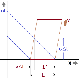
Figure 1: (Color Online) A rod moving in 1-dimension with constant velocity.

The apparent length registered by the distant observer at $x=0$ comes out to be $L^{\prime}=L-v\Delta t$; where $\Delta t$ being the time taken by light-ray from one end of the rod to other.

Solving for $L^{\prime}$ and $\Delta t$, with $L^{\prime}=c\Delta t$, we get:

$$\dfrac{L^{\prime}}{L}\ =\ \dfrac{c}{(c\ +v)}\ =\ \dfrac{1}{(1\ +\beta)}$$ (4)

Which when generalized for motion in arbitrary direction, becomes:

$$\dfrac{L^{\prime}}{L}\ =\ \dfrac{1}{(1\ -\boldsymbol{\hat{n}}\cdot\boldsymbol{\beta})}$$ (5)

While, $\boldsymbol{\hat{n}}$ being the unit vector from particle’s ’retarded’ position to the direction of the observer’s ’present’ position.

The quantity $(1\ -\boldsymbol{\hat{n}}\cdot\boldsymbol{\beta})$ or $(Rc-\textbf{R}\cdot\textbf{v})$ or $-R_{\mu}u^{\mu}$ in denominator appears purely due to apparent geometry perceived by the distant observer.

Thus, effectively, the observer perceives retarded charge and current densities in-access or less than the actual, depending upon the particle’s velocity vector. [5]

However, when the same logic were extended to the accelerating rod, the picture gets distorted further; as the observer would see different parts of the rod travelling with different velocities. This may be visualized from figure- 2 below:

Figure 2: (Color Online) Accelerating rod in 1-dimension.

Assuming the rod moving with low enough velocities ( $v<<c$ ) and acceleration ( $a\Delta t<<c$ ), non-relativistic (Newtonian) equations of motion would hold good. Further assuming the rod to be rigid (i.e. not getting deformed under the stresses developed by acceleration), the distorted length as perceived by the observer now comes:

$$L^{\prime}\ =L\ -v_{1}\Delta t\ -\dfrac{a}{2}\Delta t^{2}\ =L\ -\dfrac{(v_{1}\ +v_{2})}{2}\Delta t$$ (6)

Though, it seems that for a point-particle, for which $L\ \approx 0$, $v_{1}\rightarrow v_{2}$; and the expressions for LW potentials (2) would remain unchanged; but actually, the things come out to be different in case the particle were spinning.

The next section demonstrates the same for an spinning sphere.

3 Effect of Acceleration and Spin on apparent geometry of a point-sphere:

Considering a spherical volume charge distribution of overall charge $q$, radius $r_{q}$ and spinning with spin-angular-velocity pseudo-vector $\boldsymbol{\omega_{s}}$. The center of the charged-sphere were moving with velocity v in positive Z-direction, and being acted upon by an external force, causing it to accelerate. The instantaneous acceleration being a.

Considering an infinitesimal volume-element $r^{2}d\Omega dr$ at position $r$ on the sphere, with reference to its center, ( $dr$ being the thickness, and $d\Omega$ being the solid-angle that the volume-element subtends at the center of the sphere) as in figure- 3:

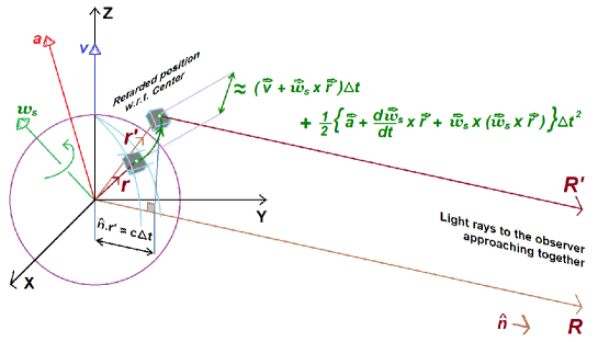
Figure 3: (Color Online) Spinning point sphere in arbitrary motion.

Due to linear and rotational velocities and accelerations, with reference to the center of the sphere, the volume-element would be subjected to retardation.

Thus, the instance when a faraway observer registers a light-ray from the center of the sphere, the ray that arrives from the volume-element seems to have come from a slightly displaced position r’.

While, the amount of retardation satisfies the equation:

$$c\Delta t\ =\boldsymbol{\hat{n}}\cdot\textbf{r'}$$ (7)

Where, $\Delta t$ is the coordinate-time difference in which the volume-element moves from position r to r’; and $\boldsymbol{\hat{n}}$ is the unit-vector pointing in the direction of faraway observer.

If $\textbf{v}(\textbf{r})$ and $\textbf{a}(\textbf{r})$ being the net velocity and acceleration of the volume-element at position r, respectively; the retarded-position r’ and velocity at retarded-position $\textbf{v}(\textbf{r'})$, are evaluated using the Taylor series as:

$$\textbf{r'}\ =\textbf{r}\ +\textbf{v}(\textbf{r})\Delta t\ +\dfrac{1}{2}\textbf{a}(\textbf{r})\Delta t^{2}\ +\dfrac{1}{6}\boldsymbol{\dot{a}}(\textbf{r})\Delta t^{3}\ +\cdots\cdots$$ (8)

And,

$$\textbf{v}(\textbf{r'})\ =\textbf{v}(\textbf{r})\ +\textbf{a}(\textbf{r})\Delta t\ +\dfrac{1}{2}\boldsymbol{\dot{a}}(\textbf{r})\Delta t^{2}\ +\dfrac{1}{6}\boldsymbol{\ddot{a}}(\textbf{r})\Delta t^{3}\ +\cdots\cdots$$ (9)

Where, $\boldsymbol{\dot{a}}(\textbf{r})\ =d\textbf{a}(\textbf{r})/dt_{ret}$ and $\boldsymbol{\ddot{a}}(\textbf{r})\ =d^{2}\textbf{a}(\textbf{r})/dt_{ret}^{2}$ being the acceleration and jerk of the volume-element, respectively, evaluated at retarded time $t_{ret}$.

Further, with consideration of spin into account and with assumption that the charged-sphere is rigid (so that it doesn’t deform due to acceleration and twist), $\textbf{v}(\textbf{r})$ would be the sum of velocity of the center and rotational velocity of the volume-element with respect to the center; which is given by:

$$\textbf{v}(\textbf{r})\ =\textbf{v}\ +\boldsymbol{\omega_{s}}\times\textbf{r}$$ (10)

From, $\textbf{v}(\textbf{r})$ above, $\textbf{a}(\textbf{r})$ may be evaluated as:

$$\begin{matrix}\textbf{a}(\textbf{r})&\ =\dfrac{d\textbf{v}(\textbf{r})}{dt_{ret}}&\ =&\textbf{a}\ +\dfrac{d\boldsymbol{\omega_{s}}}{dt_{ret}}\times\textbf{r}\ +\boldsymbol{\omega_{s}}\times(\boldsymbol{\omega_{s}}\times\textbf{r})\\ {}&{}&{}&{}\\ {}&{}&\ =&\textbf{a}\ +\boldsymbol{\dot{\omega}_{s}}\times\textbf{r}\ +\left\{(\boldsymbol{\omega_{s}}\cdot\textbf{r})\boldsymbol{\omega_{s}}\ -{\omega_{s}}^{2}\textbf{r}\right\}\end{matrix}$$ (11)

The first term in equation (11) is instantaneous linear acceleration of sphere’s center; the second term is the acceleration component due to angular-acceleration; and the third-term is centrifugal-acceleration.

Further, the jerk on the volume-element at position r may be evaluated as:

$$\begin{matrix}\boldsymbol{\dot{a}}(\textbf{r})&\ =&\dfrac{d\textbf{a}(\textbf{r})}{dt_{ret}}\\ {}&{}&{}\\ {}&\ =&\dfrac{d\textbf{a}}{dt_{ret}}\ +\dfrac{d^{2}\boldsymbol{\omega_{s}}}{dt_{ret}^{2}}\times\textbf{r}\ +2\dfrac{d\boldsymbol{\omega_{s}}}{dt_{ret}}\times\left(\boldsymbol{\omega_{s}}\times\textbf{r}\right)\ +\boldsymbol{\omega_{s}}\times\left(\dfrac{d\boldsymbol{\omega_{s}}}{dt_{ret}}\times\textbf{r}\right)\\ {}&{}&{}\\ {}&{}&\ +\boldsymbol{\omega_{s}}\times\left\{\boldsymbol{\omega_{s}}\times(\boldsymbol{\omega_{s}}\times\textbf{r})\right\}\\ {}&{}&{}\\ {}&\ =&\boldsymbol{\dot{a}}\ +\boldsymbol{\ddot{\omega}_{s}}\times\textbf{r}\ +2\boldsymbol{\dot{\omega}_{s}}\times\left(\boldsymbol{\omega_{s}}\times\textbf{r}\right)\ +\boldsymbol{\omega_{s}}\times\left(\boldsymbol{\dot{\omega}_{s}}\times\textbf{r}\right)\\ {}&{}&{}\\ {}&{}&\ -{\omega_{s}}^{2}(\boldsymbol{\omega_{s}}\times\textbf{r})\end{matrix}$$ (12)

If R is the vector distance of the faraway observer from center of the point-charge, the vector distance of the observer from retarded position of the volume-element is given by:

$$\textbf{R'}\ =\textbf{R}\ -\textbf{r'}$$ (13)

And, scalar-distance $R^{\prime}$ is given by:

$$R^{\prime}\ =\sqrt{(}R^{2}\ +r^{\prime 2}\ -2\textbf{R}\cdot\textbf{r'})\ =R\left\{1\ +\dfrac{r^{\prime 2}}{R^{2}}\ -\dfrac{2}{R}(\boldsymbol{\hat{n}}\cdot\textbf{r'})\right\}^{\frac{1}{2}}$$ (14)

Equations (8), (9), (13) and (14) indicate that the apparent retardation sensed by a distant observer is different for different positions r on the sphere.

Thus, in-line with equations (2) and (3), the overall LW 4-potentials due to the entire charged-sphere may be evaluated by:

$$\begin{matrix}A^{\mu}(R^{\mu})&\ =&\lim_{r_{q}\to\ 0}\dfrac{\rho}{4\pi\epsilon_{0}c^{2}}\int_{r}\iint_{\Omega}\dfrac{u^{\mu}(\textbf{r'})}{\left\{-R^{\prime}_{\mu}u^{\mu}(\textbf{r'})\right\}}r^{2}d\Omega dr\\ {}&{}&{}\\ {}&\ =&\lim_{r_{q}\to\ 0}\dfrac{\rho}{4\pi\epsilon_{0}c^{2}}\int_{r}r^{2}dr\iint_{\Omega}\dfrac{\langle\langle c;\ \textbf{v}(\textbf{r'})\rangle\rangle\ d\Omega}{\left\{R^{\prime}c\ -\textbf{R'}\cdot\textbf{v}(\textbf{r'})\right\}}\end{matrix}$$ (15)

Where $\rho$, is the ’rest’ charge-density of the point-charge,

Equation (15) indicates that to evaluate LW potentials, the 4-vector terms $u^{\mu}(\textbf{r'})/\left\{-R^{\prime}_{\mu}u^{\mu}(\textbf{r'})\right\}$ for the volume-element are to be evaluated first.

Next sections is devoted to the same.

4 LW 4-Potentials due to Spinning Point-Charge in motion:

From equation (7), $\Delta t$ seems to be of the order of $r^{\prime}/c$. In non-relativistic limit, i.e. for ’slow enough’ velocity and acceleration ( $v<<c$, $a\Delta t<<c$ ), $r^{\prime}$ approaches $r$.

Further, $r$ being the radius of point-particle, is too small as compared to the distance from the observer (i.e. $r<<R$). Thus, in point-particle limit $r_{q}\rightarrow 0$, $\Delta t$ would also be negligibly small; and $\Delta t\approx r/c$.

However, as the order of classical-spin goes as $r^{2}$, to examine spin dependence of LW potentials, terms of, at least, the order $\Delta t^{2}$ would need to be considered in our approximation.

Thus, from equations (8) and (9), approximated to the second powers of $\Delta t$, the apparent retardation, and the apparent velocity at retarded position as sensed by the faraway observer become:

$$\textbf{r'}\ \approx\textbf{r}\ +\textbf{v}(\textbf{r})\Delta t\ +\dfrac{1}{2}\textbf{a}(\textbf{r})\Delta t^{2}$$ (16)

And,

$$\textbf{v}(\textbf{r'})\ \approx\textbf{v}(\textbf{r})\ +\textbf{a}(\textbf{r})\Delta t\ +\dfrac{1}{2}\boldsymbol{\dot{a}}(\textbf{r})\Delta t^{2}$$ (17)

From (13) and (14), along with (16) and (17), expanding the square-root term of (14) by binomial theorem, and keeping the terms only up to like $r^{2}$ (i.e. up to $r^{2}$, $r\Delta t$ and $\Delta t^{2}$ ) , the quantity in denominator of (15) $-R^{\prime}_{\mu}u^{\mu}(\textbf{r'})$ may be evaluated as:

$$\begin{matrix}-R^{\prime}_{\mu}u^{\mu}(\textbf{r'})&\ =&R^{\prime}c\ -\textbf{R'}\cdot\textbf{v}(\textbf{r'})\\ {}&{}&{}\\ {}&\ =&R\left[\ c\ -\boldsymbol{\hat{n}}\cdot\textbf{v}(\textbf{r})\ -\left\{\boldsymbol{\hat{n}}\cdot\textbf{a}(\textbf{r})\right\}\Delta t\ -\dfrac{1}{2}\left\{\boldsymbol{\hat{n}}\cdot\boldsymbol{\dot{a}}(\textbf{r})\right\}\Delta t^{2}\right]\\ {}&{}&{}\\ {}&{}&\ +\left[\ \left\{\textbf{r}\cdot\textbf{v}(\textbf{r})\right\}\ -c(\boldsymbol{\hat{n}}\cdot\textbf{r})\ -c\left\{\boldsymbol{\hat{n}}\cdot\textbf{v}(\textbf{r})\right\}\Delta t\ +\left\{\textbf{v}(\textbf{r})\right\}^{2}\Delta t\right.\\ {}&{}&\left.\ +\left\{\textbf{r}\cdot\textbf{a}(\textbf{r})\right\}\Delta t\ -\dfrac{c}{2}\left\{\boldsymbol{\hat{n}}\cdot\textbf{a}(\textbf{r})\right\}\ +\dfrac{3}{2}\left\{\textbf{v}(\textbf{r})\cdot\textbf{a}(\textbf{r})\right\}\right]\\ {}&{}&{}\\ {}&{}&\ +\dfrac{c}{R}\left[\ \dfrac{r^{2}}{2}\ -\left\{\textbf{r}\cdot\textbf{v}(\textbf{r})\right\}\Delta t\ +\dfrac{1}{2}\left\{\textbf{v}(\textbf{r})\right\}^{2}\Delta t^{2}\right.\\ {}&{}&\left.\ -\dfrac{1}{2}\left\{\boldsymbol{\hat{n}}\cdot\textbf{v}(\textbf{r})\right\}^{2}\Delta t^{2}\ -\dfrac{1}{2}(\boldsymbol{\hat{n}}\cdot\textbf{r})^{2}\ -\left\{\boldsymbol{\hat{n}}\cdot\textbf{v}(\textbf{r})\right\}(\boldsymbol{\hat{n}}\cdot\textbf{r})\Delta t\right]\end{matrix}$$ (18)

Meanwhile, $\Delta t$ may be evaluated by using equation (16) in (7), which yields a quadratic equation in $\Delta t$:

$$\dfrac{1}{2}\left\{\boldsymbol{\hat{n}}\cdot\textbf{a}(\textbf{r})\right\}\Delta t^{2}\ -\left\{c\ -\boldsymbol{\hat{n}}\cdot\textbf{v}(\textbf{r})\right\}\Delta t\ +\boldsymbol{\hat{n}}\cdot\textbf{r}\ =0$$ (19)

The solution of which comes out to be:

$$\Delta t\ =\dfrac{\left\{c\ -\boldsymbol{\hat{n}}\cdot\textbf{v}(\textbf{r})\right\}}{\boldsymbol{\hat{n}}\cdot\textbf{a}(\textbf{r})}\ \pm\dfrac{1}{\boldsymbol{\hat{n}}\cdot\textbf{a}(\textbf{r})}\sqrt{\left[\left\{c\ -\boldsymbol{\hat{n}}\cdot\textbf{v}(\textbf{r})\right\}^{2}\ -2\left\{\boldsymbol{\hat{n}}\cdot\textbf{a}(\textbf{r})\right\}(\boldsymbol{\hat{n}}\cdot\textbf{r})\right]}$$ (20)

As $\Delta t$ must vanish at $r\ =0$, -ive sign is appropriate. Expanding the square-root with binomial theorem, we get the expression for $\Delta t$, approximated up to $r^{2}$ terms as:

$$\Delta t\ \approx\dfrac{(\boldsymbol{\hat{n}}\cdot\textbf{r})}{\left\{c\ -\boldsymbol{\hat{n}}\cdot\textbf{v}(\textbf{r})\right\}}\ +\dfrac{1}{2}\dfrac{(\boldsymbol{\hat{n}}\cdot\textbf{r})^{2}\left\{\boldsymbol{\hat{n}}\cdot\textbf{a}(\textbf{r})\right\}}{\left\{c\ -\boldsymbol{\hat{n}}\cdot\textbf{v}(\textbf{r})\right\}^{3}}$$ (21)

Using expression of $\Delta t$ of equation (21) in equation (17), velocity of the volume-element at retarded position r’, approximated up to $r^{2}$ terms, comes out to be:

$$\textbf{v}(\textbf{r'})\ \approx\textbf{v}(\textbf{r})\ +\dfrac{(\boldsymbol{\hat{n}}\cdot\textbf{r})\textbf{a}(\textbf{r})}{\left\{c\ -\boldsymbol{\hat{n}}\cdot\textbf{v}(\textbf{r})\right\}}\ +\dfrac{1}{2}\dfrac{(\boldsymbol{\hat{n}}\cdot\textbf{r})^{2}\left\{\boldsymbol{\hat{n}}\cdot\textbf{a}(\textbf{r})\right\}\textbf{a}(\textbf{r})}{\left\{c\ -\boldsymbol{\hat{n}}\cdot\textbf{v}(\textbf{r})\right\}^{3}}\ +\dfrac{1}{2}\dfrac{(\boldsymbol{\hat{n}}\cdot\textbf{r})^{2}\boldsymbol{\dot{a}}(\textbf{r})}{\left\{c\ -\boldsymbol{\hat{n}}\cdot\textbf{v}(\textbf{r})\right\}^{2}}$$ (22)

Using equations (10), (11) and (12) in (22) and up to the $r^{2}$ terms, we get:

$$\begin{matrix}\boldsymbol{v}(\textbf{r'})&\ \approx\ \textbf{v}\ +\boldsymbol{\omega_{s}}\times\textbf{r}\ +\dfrac{(\boldsymbol{\hat{n}}\cdot\textbf{r})\textbf{a}}{(c\ -\boldsymbol{\hat{n}}\cdot\textbf{v})}\ +\dfrac{(\boldsymbol{\hat{n}}\cdot\textbf{r})(\textbf{r}\cdot\langle\boldsymbol{\hat{n}}\times\boldsymbol{\omega_{s}}\rangle)\textbf{a}}{(c\ -\boldsymbol{\hat{n}}\cdot\textbf{v})^{2}}\ -\dfrac{(\boldsymbol{\hat{n}}\cdot\textbf{r})(\textbf{r}\times\boldsymbol{\dot{\omega}_{s}})}{(c\ -\boldsymbol{\hat{n}}\cdot\textbf{v})}\\ {}&{}\\ {}&\ +\dfrac{(\boldsymbol{\hat{n}}\cdot\textbf{r})(\boldsymbol{\omega_{s}}\cdot\textbf{r})\boldsymbol{\omega_{s}}}{(c\ -\boldsymbol{\hat{n}}\cdot\textbf{v})}\ -\dfrac{(\boldsymbol{\hat{n}}\cdot\textbf{r}){\omega_{s}}^{2}\textbf{r}}{(c\ -\boldsymbol{\hat{n}}\cdot\textbf{v})}\ +\dfrac{1}{2}\dfrac{(\boldsymbol{\hat{n}}\cdot\textbf{r})^{2}\left\{\boldsymbol{\hat{n}}\cdot\textbf{a}\right\}\textbf{a}}{(c\ -\boldsymbol{\hat{n}}\cdot\textbf{v})^{3}}\ +\dfrac{1}{2}\dfrac{(\boldsymbol{\hat{n}}\cdot\textbf{r})^{2}\boldsymbol{\dot{a}}}{(c\ -\boldsymbol{\hat{n}}\cdot\textbf{v})^{2}}\end{matrix}$$ (23)

Further, using expression of $\Delta t$ from equation (21), and inverting equation (18) with binomial-expansion in fractions of $\left\{c\ -\boldsymbol{\hat{n}}\cdot\textbf{v}(\textbf{r})\right\}$, up to $r^{2}$ like terms; we get:

$$\begin{matrix}\dfrac{1}{\left\{-R^{\prime}_{\mu}u^{\mu}(\textbf{r'})\right\}}&\ \approx\dfrac{1}{R}\left[\ \dfrac{1}{\left\{c\ -\boldsymbol{\hat{n}}\cdot\textbf{v}(\textbf{r})\right\}}\ +\dfrac{\left\{\boldsymbol{\hat{n}}\cdot\textbf{a}(\textbf{r})\right\}(\boldsymbol{\hat{n}}\cdot\textbf{r})}{\left\{c\ -\boldsymbol{\hat{n}}\cdot\textbf{v}(\textbf{r})\right\}^{3}}\ +\dfrac{3}{2}\dfrac{\left\{\boldsymbol{\hat{n}}\cdot\textbf{a}(\textbf{r})\right\}^{2}(\boldsymbol{\hat{n}}\cdot\textbf{r})^{2}}{\left\{c\ -\boldsymbol{\hat{n}}\cdot\textbf{v}(\textbf{r})\right\}^{5}}\right.\\ \\ {}&\left.\ +\dfrac{1}{2}\dfrac{\left\{\boldsymbol{\hat{n}}\cdot\textbf{a}(\textbf{r})\right\}(\boldsymbol{\hat{n}}\cdot\textbf{r})^{2}}{\left\{c\ -\boldsymbol{\hat{n}}\cdot\textbf{v}(\textbf{r})\right\}^{4}}\right]\\ {}&{}\\ {}&\ +\dfrac{1}{R^{2}}\left[\ \dfrac{c^{2}(\boldsymbol{\hat{n}}\cdot\textbf{r})}{\left\{c\ -\boldsymbol{\hat{n}}\cdot\textbf{v}(\textbf{r})\right\}^{3}}\ -\dfrac{\left\{\textbf{r}\cdot\textbf{v}(\textbf{r})\right\}}{\left\{c\ -\boldsymbol{\hat{n}}\cdot\textbf{v}(\textbf{r})\right\}^{2}}\ +\dfrac{5c^{2}}{2}\dfrac{\left\{\boldsymbol{\hat{n}}\cdot\textbf{a}(\textbf{r})\right\}(\boldsymbol{\hat{n}}\cdot\textbf{r})^{2}}{\left\{c\ -\boldsymbol{\hat{n}}\cdot\textbf{v}(\textbf{r})\right\}^{5}}\right.\\ \\ {}&\left.\ -\dfrac{\left\{\textbf{v}(\textbf{r})\right\}^{2}(\boldsymbol{\hat{n}}\cdot\textbf{r})}{\left\{c\ -\boldsymbol{\hat{n}}\cdot\textbf{v}(\textbf{r})\right\}^{3}}\ -\dfrac{2\left\{\boldsymbol{\hat{n}}\cdot\textbf{a}(\textbf{r})\right\}\left\{\textbf{r}\cdot\textbf{v}(\textbf{r})\right\}(\boldsymbol{\hat{n}}\cdot\textbf{r})}{\left\{c\ -\boldsymbol{\hat{n}}\cdot\textbf{v}(\textbf{r})\right\}^{3}}\right.\\ \\ {}&\left.\ -\dfrac{\left\{\textbf{r}\cdot\textbf{a}(\textbf{r})\right\}(\boldsymbol{\hat{n}}\cdot\textbf{r})}{\left\{c\ -\boldsymbol{\hat{n}}\cdot\textbf{v}(\textbf{r})\right\}^{3}}\ -\dfrac{5}{2}\dfrac{\left\{\textbf{v}(\textbf{r})\right\}^{2}\left\{\boldsymbol{\hat{n}}\cdot\textbf{a}(\textbf{r})\right\}(\boldsymbol{\hat{n}}\cdot\textbf{r})^{2}}{\left\{c\ -\boldsymbol{\hat{n}}\cdot\textbf{v}(\textbf{r})\right\}^{5}}\ -\dfrac{3}{2}\dfrac{\left\{\textbf{v}(\textbf{r})\cdot\textbf{a}(\textbf{r})\right\}(\boldsymbol{\hat{n}}\cdot\textbf{r})^{2}}{\left\{c\ -\boldsymbol{\hat{n}}\cdot\textbf{v}(\textbf{r})\right\}^{4}}\right]\\ {}&{}\\ {}&\ +\dfrac{c}{R^{3}}\left[\ \dfrac{\left\{\textbf{r}\cdot\textbf{v}(\textbf{r})\right\}(\boldsymbol{\hat{n}}\cdot\textbf{r})}{\left\{c\ -\boldsymbol{\hat{n}}\cdot\textbf{v}(\textbf{r})\right\}^{3}}\ -\dfrac{1}{2}\dfrac{r^{2}}{\left\{c\ -\boldsymbol{\hat{n}}\cdot\textbf{v}(\textbf{r})\right\}^{2}}\ -\dfrac{1}{2}\dfrac{\left\{\textbf{v}(\textbf{r})\right\}^{2}(\boldsymbol{\hat{n}}\cdot\textbf{r})^{2}}{\left\{c\ -\boldsymbol{\hat{n}}\cdot\textbf{v}(\textbf{r})\right\}^{4}}\right.\\ \\ {}&\left.\ +\dfrac{c^{2}}{2}\dfrac{(\boldsymbol{\hat{n}}\cdot\textbf{r})^{2}}{\left\{c\ -\boldsymbol{\hat{n}}\cdot\textbf{v}(\textbf{r})\right\}^{4}}\ -\dfrac{2c\left\{\textbf{r}\cdot\textbf{v}(\textbf{r})\right\}(\boldsymbol{\hat{n}}\cdot\textbf{r})}{\left\{c\ -\boldsymbol{\hat{n}}\cdot\textbf{v}(\textbf{r})\right\}^{4}}\ +\dfrac{2c\left\{\boldsymbol{\hat{n}}\cdot\textbf{v}(\textbf{r})\right\}(\boldsymbol{\hat{n}}\cdot\textbf{r})^{2}}{\left\{c\ -\boldsymbol{\hat{n}}\cdot\textbf{v}(\textbf{r})\right\}^{4}}\right.\\ \\ {}&\left.\ -\dfrac{2c\left\{\textbf{v}(\textbf{r})\right\}^{2}(\boldsymbol{\hat{n}}\cdot\textbf{r})^{2}}{\left\{c\ -\boldsymbol{\hat{n}}\cdot\textbf{v}(\textbf{r})\right\}^{5}}\ -\dfrac{2\left\{\textbf{v}(\textbf{r})\right\}^{2}\left\{\textbf{r}\cdot\textbf{v}(\textbf{r})\right\}(\boldsymbol{\hat{n}}\cdot\textbf{r})}{\left\{c\ -\boldsymbol{\hat{n}}\cdot\textbf{v}(\textbf{r})\right\}^{4}}\right]\end{matrix}$$ (24)

Now, inserting spin dependent quantities by using equations (10), (11) and (12), in (24), and carrying out binomial-expansion of the denominator in fractions of $\left\{c\ -\boldsymbol{\hat{n}}\cdot\textbf{v}\right\}$, and keeping the terms up to $r^{2}$, we get:

$$\begin{matrix}\dfrac{1}{\left\{-R^{\prime}_{\mu}u^{\mu}(\textbf{r'})\right\}}\ \approx\dfrac{1}{R}\left[\dfrac{1}{(c\ -\boldsymbol{\hat{n}}\cdot\textbf{v})}\left\{1\ +\dfrac{\boldsymbol{\hat{n}}\cdot\langle\textbf{r}\times\boldsymbol{\omega_{s}}\rangle}{(c\ -\boldsymbol{\hat{n}}\cdot\textbf{v})}\ +\dfrac{(\boldsymbol{\hat{n}}\cdot\langle\textbf{r}\times\boldsymbol{\omega_{s}}\rangle)^{2}}{(c\ -\boldsymbol{\hat{n}}\cdot\textbf{v})^{2}}\right\}\right.\\ \\ \left.\ +\dfrac{(\boldsymbol{\hat{n}}\cdot\textbf{r})}{(c\ -\boldsymbol{\hat{n}}\cdot\textbf{v})^{3}}\left\{\boldsymbol{\hat{n}}\cdot\left(\textbf{a}\ +{\boldsymbol{\dot{\omega}_{s}}\times\textbf{r}}\ +(\boldsymbol{\omega_{s}}\cdot\textbf{r})\boldsymbol{\omega_{s}}\ -{\omega_{s}}^{2}\textbf{r}\right)\right\}\left\{1\ +\dfrac{3(\boldsymbol{\hat{n}}\cdot\langle\boldsymbol{\omega_{s}}\times\textbf{r}\rangle)}{(c\ -\boldsymbol{\hat{n}}\cdot\textbf{v})}\right\}\right.{}\\ {}\\ \left.\ +\dfrac{3}{2}\dfrac{(\boldsymbol{\hat{n}}\cdot\textbf{a})^{2}(\boldsymbol{\hat{n}}\cdot\textbf{r})^{2}}{(c\ -\boldsymbol{\hat{n}}\cdot\textbf{v})^{5}}\ +\dfrac{1}{2}\dfrac{(\boldsymbol{\hat{n}}\cdot\textbf{a})(\boldsymbol{\hat{n}}\cdot\textbf{r})^{2}}{(c\ -\boldsymbol{\hat{n}}\cdot\textbf{v})^{4}}\right]{}\\ {}\\ \ +\dfrac{1}{R^{2}}\left[{c^{2}(\boldsymbol{\hat{n}}\cdot\textbf{r})}{(c\ -\boldsymbol{\hat{n}}\cdot\textbf{v})^{3}}\left\{1\ +\dfrac{3(\boldsymbol{\hat{n}}\cdot\langle\boldsymbol{\omega_{s}}\times\textbf{r}\rangle)}{(c\ -\boldsymbol{\hat{n}}\cdot\textbf{v})}\right\}\right.{}\\ {}\\ \left.\ -\dfrac{1}{(c\ -\boldsymbol{\hat{n}}\cdot\textbf{v})^{2}}\left\{\textbf{r}\cdot(\textbf{v}\ +\boldsymbol{\omega_{s}}\times\textbf{r})\right\}\left\{1\ +\dfrac{2(\boldsymbol{\hat{n}}\cdot\langle\boldsymbol{\omega_{s}}\times\textbf{r}\rangle)}{(c\ -\boldsymbol{\hat{n}}\cdot\textbf{v})}\right\}\right.{}\\ {}\\ \left.\ +\dfrac{5c^{2}}{2}\dfrac{(\boldsymbol{\hat{n}}\cdot\textbf{a})(\boldsymbol{\hat{n}}\cdot\textbf{r})^{2}}{(c\ -\boldsymbol{\hat{n}}\cdot\textbf{v})^{5}}\ -\dfrac{(\boldsymbol{\hat{n}}\cdot\textbf{r})}{(c\ -\boldsymbol{\hat{n}}\cdot\textbf{v})^{3}}\left\{\textbf{v}\ +\boldsymbol{\omega_{s}}\times\textbf{r}\right\}^{2}\left\{1\ +\dfrac{3(\boldsymbol{\hat{n}}\cdot\langle\boldsymbol{\omega_{s}}\times\textbf{r}\rangle)}{(c\ -\boldsymbol{\hat{n}}\cdot\textbf{v})}\right\}\right.{}\\ {}\\ \left.\ -\dfrac{2(\boldsymbol{\hat{n}}\cdot\textbf{a})(\textbf{r}\cdot\textbf{v})(\boldsymbol{\hat{n}}\cdot\textbf{r})}{(c\ -\boldsymbol{\hat{n}}\cdot\textbf{v})^{3}}\ -\dfrac{(\textbf{r}\cdot\textbf{a})(\boldsymbol{\hat{n}}\cdot\textbf{r})}{(c\ -\boldsymbol{\hat{n}}\cdot\textbf{v})^{3}}\ -\dfrac{5}{2}\dfrac{v^{2}(\boldsymbol{\hat{n}}\cdot\textbf{a})(\boldsymbol{\hat{n}}\cdot\textbf{r})^{2}}{(c\ -\boldsymbol{\hat{n}}\cdot\textbf{v})^{5}}\ -\dfrac{3}{2}\dfrac{(\textbf{v}\cdot\textbf{a})(\boldsymbol{\hat{n}}\cdot\textbf{r})^{2}}{(c\ -\boldsymbol{\hat{n}}\cdot\textbf{v})^{4}}\right]{}\\ {}\\ \ +\dfrac{c}{R^{3}}\left[\dfrac{(\textbf{r}\cdot\textbf{v})(\boldsymbol{\hat{n}}\cdot\textbf{r})}{(c\ -\boldsymbol{\hat{n}}\cdot\textbf{v})^{3}}\ -\dfrac{1}{2}\dfrac{r^{2}}{(c\ -\boldsymbol{\hat{n}}\cdot\textbf{v})^{2}}\ -\dfrac{1}{2}\dfrac{v^{2}(\boldsymbol{\hat{n}}\cdot\textbf{r})^{2}}{(c\ -\boldsymbol{\hat{n}}\cdot\textbf{v})^{4}}\ +\dfrac{c^{2}}{2}\dfrac{(\boldsymbol{\hat{n}}\cdot\textbf{r})^{2}}{(c\ -\boldsymbol{\hat{n}}\cdot\textbf{v})^{4}}\right.{}\\ {}\\ \left.\ -\dfrac{2c(\textbf{r}\cdot\textbf{v})(\boldsymbol{\hat{n}}\cdot\textbf{r})}{(c\ -\boldsymbol{\hat{n}}\cdot\textbf{v})^{4}}\ +\dfrac{2c(\boldsymbol{\hat{n}}\cdot\textbf{v})(\boldsymbol{\hat{n}}\cdot\textbf{r})^{2}}{(c\ -\boldsymbol{\hat{n}}\cdot\textbf{v})^{4}}\ -\dfrac{2cv^{2}(\boldsymbol{\hat{n}}\cdot\textbf{r})^{2}}{(c\ -\boldsymbol{\hat{n}}\cdot\textbf{v})^{5}}\ -\dfrac{2v^{2}(\textbf{r}\cdot\textbf{v})(\boldsymbol{\hat{n}}\cdot\textbf{r})}{(c\ -\boldsymbol{\hat{n}}\cdot\textbf{v})^{4}}\right]\end{matrix}$$ (25)

Now LW Potentials may be evaluated easily by evaluating $u^{\mu}(\textbf{r'})/\left\{-R^{\prime}_{\mu}u^{\mu}(\textbf{r'})\right\}$ from product of equations (25) above, and (23), putting the same in equation (15), performing integration over the entire volume of the sphere, and applying the limit $r_{q}toward0$.

Though, it is expected that the expression of 4-vector $u^{\mu}(\textbf{r'})/\left\{-R^{\prime}_{\mu}u^{\mu}(\textbf{r'})\right\}$ such obtained, would be too lengthy; by inspection of terms and making use of known spherical integrals, and analyzing the terms in context of limit $r_{q}\rightarrow 0$, many terms may be eliminated and need not be written down.

Following are the known spherical integrals:

$$\left.\begin{matrix}\iint_{\Omega}(\textbf{r}\cdot\textbf{A})d\Omega\ =0;\\ \\ \iint_{\Omega}(\textbf{r}\times\textbf{A})d\Omega\ =0;\\ \\ \iint_{\Omega}(\textbf{r}\cdot\textbf{A})(\textbf{r}\cdot\textbf{B})d\Omega\ =\dfrac{4\pi}{3}r^{2}(\textbf{A}\cdot\textbf{B});\\ \\ \iint_{\Omega}(\textbf{r}\cdot\textbf{A})(\textbf{r}\times\textbf{B})d\Omega\ =\dfrac{4\pi}{3}r^{2}(\textbf{A}\times\textbf{B});\\ \\ \iint_{\Omega}(\textbf{r}\cdot\textbf{A})\textbf{r}d\Omega\ =\dfrac{4\pi}{3}r^{2}\textbf{A};\end{matrix}\ \right\}$$ (26)

It can be seen from equations (26) that the spherical-integrals of terms that contain single $r$ vanish. Further, the terms that contain $r$ but are without $\omega_{s}$ would go to 0, when the limit $r_{q}\rightarrow 0$ were applied

Thus, identifying and writing only non-vanishing terms from product of equations (25) and (23), and putting them in (16), expression of LW 4-potentials may be simplified as:

$$\begin{matrix}A^{\mu}(R^{\mu})\ =\lim_{r_{q}\to\ 0}\dfrac{\rho}{4\pi\epsilon_{0}c^{2}}\int_{r}r^{2}dr\iint_{\Omega}\left[\dfrac{\left\langle\left\langle c;\ \textbf{v}\right\rangle\right\rangle}{R}\left\{\dfrac{1}{(c\ -\boldsymbol{\hat{n}}\cdot\textbf{v})}\ +\dfrac{(\textbf{r}\cdot\langle\boldsymbol{\hat{n}}\times\boldsymbol{\omega_{s}}\rangle)^{2}}{(c\ -\boldsymbol{\hat{n}}\cdot\textbf{v})^{3}}\right.\right.{}\\ {}\\ \left.\left.\ +\dfrac{(\boldsymbol{\hat{n}}\cdot\textbf{r})(\textbf{r}\cdot\langle\boldsymbol{\hat{n}}\times\boldsymbol{\dot{\omega}_{s}}\rangle)}{(c\ -\boldsymbol{\hat{n}}\cdot\textbf{v})^{3}}\ +\dfrac{(\boldsymbol{\hat{n}}\cdot\boldsymbol{\omega_{s}})(\boldsymbol{\hat{n}}\cdot\textbf{r})(\textbf{r}\cdot\boldsymbol{\omega_{s}})}{(c\ -\boldsymbol{\hat{n}}\cdot\textbf{v})^{3}}\ -\dfrac{{\omega_{s}}^{2}(\boldsymbol{\hat{n}}\cdot\textbf{r})^{2}}{(c\ -\boldsymbol{\hat{n}}\cdot\textbf{v})^{3}}\right.\right.{}\\ {}\\ \left.\left.\ +\dfrac{3(\boldsymbol{\hat{n}}\cdot\textbf{a})(\boldsymbol{\hat{n}}\cdot\textbf{r})(\textbf{r}\cdot\langle\boldsymbol{\hat{n}}\times\boldsymbol{\omega_{s}}\rangle)}{(c\ -\boldsymbol{\hat{n}}\cdot\textbf{v})^{4}}\right\}\right.{}\\ {}\\ \left.\ +\dfrac{\left\langle\left\langle c;\ \textbf{v}\right\rangle\right\rangle}{R^{2}}\left\{\dfrac{3c^{2}(\boldsymbol{\hat{n}}\cdot\textbf{r})(\textbf{r}\cdot\langle\boldsymbol{\hat{n}}\times\boldsymbol{\omega_{s}}\rangle)}{(c\ -\boldsymbol{\hat{n}}\cdot\textbf{v})^{4}}\ -\dfrac{2(\textbf{r}\cdot\textbf{v})(\textbf{r}\cdot\langle\boldsymbol{\hat{n}}\times\boldsymbol{\omega_{s}}\rangle)}{(c\ -\boldsymbol{\hat{n}}\cdot\textbf{v})^{3}}\ -\dfrac{2(\boldsymbol{\hat{n}}\cdot\textbf{r})(\textbf{r}\cdot\langle\textbf{v}\times\boldsymbol{\omega_{s}}\rangle)}{(c\ -\boldsymbol{\hat{n}}\cdot\textbf{v})^{3}}\right.\right.{}\\ {}\\ \left.\left.\ -\dfrac{3v^{2}(\boldsymbol{\hat{n}}\cdot\textbf{r})(\textbf{r}\cdot\langle\boldsymbol{\hat{n}}\times\boldsymbol{\omega_{s}}\rangle)}{(c\ -\boldsymbol{\hat{n}}\cdot\textbf{v})^{4}}\right\}\right.{}\\ {}\\ \left.\ -\dfrac{\left\langle\left\langle 0;\ \textbf{r}\times\boldsymbol{\omega_{s}}\right\rangle\right\rangle}{R}\left\{\dfrac{(\boldsymbol{\hat{n}}\cdot\textbf{r})}{(c\ -\boldsymbol{\hat{n}}\cdot\textbf{v})^{2}}\ +\dfrac{(\textbf{r}\cdot\langle\boldsymbol{\hat{n}}\times\boldsymbol{\omega_{s}}\rangle)}{(c\ -\boldsymbol{\hat{n}}\cdot\textbf{v})^{2}}\ +\dfrac{(\boldsymbol{\hat{n}}\cdot\textbf{a})(\boldsymbol{\hat{n}}\cdot\textbf{r})}{(c\ -\boldsymbol{\hat{n}}\cdot\textbf{v})^{3}}\right\}\right.{}\\ {}\\ \left.\ +\dfrac{\left\langle\left\langle 0;\ \textbf{r}\times\boldsymbol{\omega_{s}}\right\rangle\right\rangle}{R^{2}}\left\{\ -\dfrac{c^{2}(\boldsymbol{\hat{n}}\cdot\textbf{r})}{(c\ -\boldsymbol{\hat{n}}\cdot\textbf{v})^{3}}\ +\dfrac{(\textbf{r}\cdot\textbf{v})}{(c\ -\boldsymbol{\hat{n}}\cdot\textbf{v})^{2}}\ +\dfrac{v^{2}(\boldsymbol{\hat{n}}\cdot\textbf{r})}{(c\ -\boldsymbol{\hat{n}}\cdot\textbf{v})^{3}}\right\}\right.{}\\ {}\\ \left.\ +\dfrac{\left\langle\left\langle 0;\ \textbf{a}\right\rangle\right\rangle}{R}\left\{\dfrac{(\boldsymbol{\hat{n}}\cdot\textbf{r})(\textbf{r}\cdot\langle\boldsymbol{\hat{n}}\times\boldsymbol{\omega_{s}}\rangle)}{(c\ -\boldsymbol{\hat{n}}\cdot\textbf{v})^{3}}\ +\dfrac{(\boldsymbol{\hat{n}}\cdot\textbf{r})(\textbf{r}\cdot\langle\boldsymbol{\hat{n}}\times\boldsymbol{\omega_{s}}\rangle)}{(c\ -\boldsymbol{\hat{n}}\cdot\textbf{v})^{3}}\right\}\right.{}\\ {}\\ \left.\ +\dfrac{1}{R}\left\{\dfrac{(\boldsymbol{\hat{n}}\cdot\textbf{r})(\textbf{r}\cdot\boldsymbol{\omega_{s}})}{(c\ -\boldsymbol{\hat{n}}\cdot\textbf{v})^{2}}{\left\langle\left\langle 0;\ \boldsymbol{\omega_{s}}\right\rangle\right\rangle}\ -\dfrac{{\omega_{s}}^{2}(\boldsymbol{\hat{n}}\cdot\textbf{r})}{(c\ -\boldsymbol{\hat{n}}\cdot\textbf{v})^{2}}{\left\langle\left\langle 0;\ \textbf{r}\right\rangle\right\rangle}\right\}\right]d\Omega\end{matrix}$$ (27)

Here, the triple product identities: $\boldsymbol{\hat{n}}\cdot\langle\boldsymbol{\omega_{s}}\times\textbf{r}\rangle\ =\textbf{r}\cdot\langle\boldsymbol{\hat{n}}\times\boldsymbol{\omega_{s}}\rangle$ and $\boldsymbol{\omega_{s}}\times\langle\boldsymbol{\omega_{s}}\times\textbf{r}\rangle\ =(\textbf{r}\cdot\boldsymbol{\omega_{s}})\boldsymbol{\omega_{s}}\ -{\omega_{s}}^{2}\textbf{r}$ have been used.

Evaluating, spherical-integrals by using set of equation (26) first, we get:

$$\begin{matrix}A^{\mu}(R^{\mu})\ =\lim_{r_{q}\to\ 0}\dfrac{\rho}{4\pi\epsilon_{0}c^{2}}\int_{r}r^{2}dr\left[\dfrac{\left\langle\left\langle c;\ \textbf{v}\right\rangle\right\rangle}{R}\left\{\dfrac{4\pi}{(c\ -\boldsymbol{\hat{n}}\cdot\textbf{v})}\ +\dfrac{4\pi r^{2}(\boldsymbol{\hat{n}}\times\boldsymbol{\omega_{s}})^{2}}{3(c\ -\boldsymbol{\hat{n}}\cdot\textbf{v})^{3}}\right.\right.\\ \\ \left.\left.\ +\dfrac{4\pi r^{2}(\boldsymbol{\hat{n}}\cdot\langle\boldsymbol{\hat{n}}\times\boldsymbol{\dot{\omega}_{s}}\rangle)}{3(c\ -\boldsymbol{\hat{n}}\cdot\textbf{v})^{3}}\ +\dfrac{4\pi r^{2}(\boldsymbol{\hat{n}}\cdot\boldsymbol{\omega_{s}})^{2}}{3(c\ -\boldsymbol{\hat{n}}\cdot\textbf{v})^{3}}\ -\dfrac{4\pi r^{2}{\omega_{s}}^{2}}{3(c\ -\boldsymbol{\hat{n}}\cdot\textbf{v})^{3}}\right.\right.\\ \\ \left.\left.\ +\dfrac{4\pi r^{2}(\boldsymbol{\hat{n}}\cdot\textbf{a})(\boldsymbol{\hat{n}}\cdot\langle\boldsymbol{\hat{n}}\times\boldsymbol{\omega_{s}}\rangle)}{(c\ -\boldsymbol{\hat{n}}\cdot\textbf{v})^{4}}\right\}\right.\\ \\ \left.\ +\dfrac{\left\langle\left\langle c;\ \textbf{v}\right\rangle\right\rangle}{R^{2}}\left\{\dfrac{4\pi r^{2}c^{2}(\boldsymbol{\hat{n}}\cdot\langle\boldsymbol{\hat{n}}\times\boldsymbol{\omega_{s}}\rangle)}{(c\ -\boldsymbol{\hat{n}}\cdot\textbf{v})^{4}}\ -\dfrac{8\pi r^{2}(\textbf{v}\cdot\langle\boldsymbol{\hat{n}}\times\boldsymbol{\omega_{s}}\rangle)}{3(c\ -\boldsymbol{\hat{n}}\cdot\textbf{v})^{3}}\ -\dfrac{8\pi r^{2}(\boldsymbol{\hat{n}}\cdot\langle\textbf{v}\times\boldsymbol{\omega_{s}}\rangle)}{3(c\ -\boldsymbol{\hat{n}}\cdot\textbf{v})^{3}}\right.\right.\\ \\ \left.\left.\ -\dfrac{4\pi r^{2}v^{2}(\boldsymbol{\hat{n}}\cdot\langle\boldsymbol{\hat{n}}\times\boldsymbol{\omega_{s}}\rangle)}{(c\ -\boldsymbol{\hat{n}}\cdot\textbf{v})^{4}}\right\}\right.\\ \\ \left.\ -\dfrac{\left\langle\left\langle 0;\ \boldsymbol{\hat{n}}\times\boldsymbol{\omega_{s}}\right\rangle\right\rangle}{R}\left\{\dfrac{4\pi r^{2}(\boldsymbol{\hat{n}}\cdot\textbf{a})}{3(c\ -\boldsymbol{\hat{n}}\cdot\textbf{v})^{3}}\right\}\right.\\ \\ \left.\ +\dfrac{\left\langle\left\langle 0;\ \boldsymbol{\hat{n}}\times\boldsymbol{\omega_{s}}\right\rangle\right\rangle}{R^{2}}\left\{\ -\dfrac{4\pi r^{2}c^{2}}{3(c\ -\boldsymbol{\hat{n}}\cdot\textbf{v})^{3}}\ +\dfrac{4\pi r^{2}v^{2}}{3(c\ -\boldsymbol{\hat{n}}\cdot\textbf{v})^{3}}\right\}\right.\\ \\ \left.\ +\dfrac{\left\langle\left\langle 0;\ \textbf{a}\right\rangle\right\rangle}{R}\left\{\dfrac{4\pi r^{2}(\boldsymbol{\hat{n}}\cdot\langle\boldsymbol{\hat{n}}\times\boldsymbol{\omega_{s}}\rangle)}{3(c\ -\boldsymbol{\hat{n}}\cdot\textbf{v})^{3}}\ +\dfrac{4\pi r^{2}(\boldsymbol{\hat{n}}\cdot\langle\boldsymbol{\hat{n}}\times\boldsymbol{\omega_{s}}\rangle)}{3(c\ -\boldsymbol{\hat{n}}\cdot\textbf{v})^{3}}\right\}\right.\\ \\ \left.\ -\dfrac{\left\langle\left\langle 0;\ \boldsymbol{\hat{n}}\times\boldsymbol{\dot{\omega}_{s}}\right\rangle\right\rangle}{R}\left\{\dfrac{4\pi r^{2}}{3(c\ -\boldsymbol{\hat{n}}\cdot\textbf{v})^{2}}\right\}\ +\dfrac{\left\langle\left\langle 0;\ \boldsymbol{\omega_{s}}\right\rangle\right\rangle}{R}\left\{\dfrac{4\pi r^{2}(\boldsymbol{\hat{n}}\cdot\boldsymbol{\omega_{s}})}{3(c\ -\boldsymbol{\hat{n}}\cdot\textbf{v})^{2}}\right\}\right.\\ \\ \left.\ -\dfrac{\left\langle\left\langle 0;\ \boldsymbol{\hat{n}}\right\rangle\right\rangle}{R}\left\{\dfrac{4\pi r^{2}{\omega_{s}}^{2}}{3(c\ -\boldsymbol{\hat{n}}\cdot\textbf{v})^{2}}\right\}\ -\dfrac{\left\langle\left\langle 0;\ \langle\boldsymbol{\hat{n}}\times\boldsymbol{\omega_{s}}\rangle\times\boldsymbol{\omega_{s}}\right\rangle\right\rangle}{R}\left\{\dfrac{4\pi r^{2}}{3(c\ -\boldsymbol{\hat{n}}\cdot\textbf{v})^{2}}\right\}\right.\\ \\ \left.\ +\dfrac{\left\langle\left\langle 0;\ \textbf{v}\times\boldsymbol{\omega_{s}}\right\rangle\right\rangle}{R^{2}}\left\{\dfrac{4\pi r^{2}}{3(c\ -\boldsymbol{\hat{n}}\cdot\textbf{v})^{2}}\right\}\right]\end{matrix}$$ (28)

All terms like $\boldsymbol{\hat{n}}\cdot(\boldsymbol{\hat{n}}\times\boldsymbol{\omega_{s}})$ vanish. Further, 2nd term cancel-out with 4th and 5th, as $(\boldsymbol{\hat{n}}\times\boldsymbol{\omega_{s}})^{2}\ ={\omega_{s}}^{2}\ -(\boldsymbol{\hat{n}}\cdot\boldsymbol{\omega_{s}})^{2}$. The 8th term cancels-out with 9th. Lastly, the 17th and 18th terms cancel-out with 19th, as $(\boldsymbol{\hat{n}}\times\boldsymbol{\omega_{s}})\times\boldsymbol{\omega_{s}}\ =-{\omega_{s}}^{2}\boldsymbol{\hat{n}}\ +(\boldsymbol{\hat{n}}\cdot\boldsymbol{\omega_{s}})\boldsymbol{\omega_{s}}$.

Thus, writing and rearranging only the surviving term out of equation (28), we have :

$$\begin{matrix}A^{\mu}(R^{\mu})\ =\lim_{r_{q}\to\ 0}\dfrac{\rho}{4\pi\epsilon_{0}c^{2}}\int_{r=0}^{r_{q}}4\pi\left[{\left\langle\left\langle c;\ \textbf{v}\right\rangle\right\rangle}\left\{\dfrac{r^{2}}{R(c\ -\boldsymbol{\hat{n}}\cdot\textbf{v})}\right\}\right.\\ \\ \left.\ -\dfrac{\left\langle\left\langle 0;\ \boldsymbol{\hat{n}}\times\boldsymbol{\omega_{s}}\right\rangle\right\rangle}{3}\left\{\dfrac{r^{4}}{R(c\ -\boldsymbol{\hat{n}}\cdot\textbf{v})^{2}}\ +\dfrac{r^{4}(\boldsymbol{\hat{n}}\cdot\textbf{a})}{R(c\ -\boldsymbol{\hat{n}}\cdot\textbf{v})^{3}}\ +\dfrac{r^{4}(c^{2}\ -v^{2})}{R^{2}(c\ -\boldsymbol{\hat{n}}\cdot\textbf{v})^{3}}\right\}\right.\\ \\ \left.\ +\dfrac{\left\langle\left\langle 0;\ \textbf{v}\times\boldsymbol{\omega_{s}}\right\rangle\right\rangle}{3}\left\{\dfrac{4\pi r^{2}}{R^{2}(c\ -\boldsymbol{\hat{n}}\cdot\textbf{v})^{2}}\right\}\right]dr\end{matrix}$$ (29)

Now, performing $r$ integrals and re-arranging the resultant terms, we get:

$$\begin{matrix}A^{\mu}(R^{\mu})\ =\lim_{r_{q}\to\ 0}\dfrac{\rho}{4\pi\epsilon_{0}c^{2}}\left(\dfrac{4}{3}\pi{r_{q}}^{3}\right)\left[\dfrac{1}{R}\left\{\dfrac{\left\langle\left\langle c;\ \textbf{v}\right\rangle\right\rangle}{(c\ -\boldsymbol{\hat{n}}\cdot\textbf{v})}\ -\dfrac{r_{q}^{2}\left\langle\left\langle 0;\ \boldsymbol{\hat{n}}\times\boldsymbol{\dot{\omega}_{s}}\right\rangle\right\rangle}{5(c\ -\boldsymbol{\hat{n}}\cdot\textbf{v})^{2}}\right.\right.\\ \\ \left.\left.\ -\dfrac{r_{q}^{2}(\boldsymbol{\hat{n}}\cdot\textbf{a}){\left\langle\left\langle 0;\ \boldsymbol{\hat{n}}\times\boldsymbol{\omega_{s}}\right\rangle\right\rangle}}{5(c\ -\boldsymbol{\hat{n}}\cdot\textbf{v})^{3}}\right\}\ +\dfrac{1}{R^{2}}\left\{\dfrac{r_{q}^{2}\left\langle\left\langle 0;\ \textbf{v}\times\boldsymbol{\omega_{s}}\right\rangle\right\rangle}{5(c\ -\boldsymbol{\hat{n}}\cdot\textbf{v})^{2}}\ -\dfrac{r_{q}^{2}(c^{2}-v^{2})\left\langle\left\langle 0;\ \boldsymbol{\hat{n}}\times\boldsymbol{\omega_{s}}\right\rangle\right\rangle}{5(c\ -\boldsymbol{\hat{n}}\cdot\textbf{v})^{3}}\right\}\right]\end{matrix}$$ (30)

$4/3\pi{r_{q}}^{3}\ \rho$ being the total charge of the sphere, in point-particle limit $r_{q}\rightarrow 0$, becomes $q$, the total charge of the point-particle.

Further, in rest of the terms, quantity $r_{q}^{2}\boldsymbol{\omega_{s}}$ may be represented in the form of particle’s spin-angular-momentum s.

Spin-Angular-Momentum of a rigid sphere is given by:

$$\textbf{s}\ =\dfrac{2}{5}m{r_{q}}^{2}\boldsymbol{\omega_{s}}$$ (31)

In point-particle limit $r_{q}\rightarrow 0$, s is known as ’Classical-spin’ of the point-particle.

Thus, with use of equation (31) in point-particle limit, writing equations (30) for $\Phi(\textbf{R},t)$ and $\textbf{A}(\textbf{R},t)$ separately, we have:

$$\Phi(\textbf{R},t)\ =\dfrac{q}{4\pi\epsilon_{0}R}\dfrac{c}{(c-\boldsymbol{\hat{n}}\cdot\textbf{v})}$$ (32)

Which is same as in equation (2); and:

$$\begin{matrix}\textbf{A}(\textbf{R},t)\ =\dfrac{q}{4\pi\epsilon_{0}c}\left[\dfrac{1}{R}\left\{\dfrac{\textbf{v}}{(c\ -\boldsymbol{\hat{n}}\cdot\textbf{v})}\ -\dfrac{(\boldsymbol{\hat{n}}\times{\boldsymbol{\dot{s}}})}{2m(c\ -\boldsymbol{\hat{n}}\cdot\textbf{v})^{2}}\ -\dfrac{(\boldsymbol{\hat{n}}\cdot\textbf{a})(\boldsymbol{\hat{n}}\times\textbf{s})}{2m(c\ -\boldsymbol{\hat{n}}\cdot\textbf{v})^{3}}\right\}\right.\\ \\ \left.\ +\dfrac{1}{R^{2}}\left\{\dfrac{(\textbf{v}\times\textbf{s})}{2m(c\ -\boldsymbol{\hat{n}}\cdot\textbf{v})^{2}}\ -\dfrac{(c^{2}-v^{2})(\boldsymbol{\hat{n}}\times\textbf{s})}{2(c\ -\boldsymbol{\hat{n}}\cdot\textbf{v})^{3}}\right\}\right]\end{matrix}$$ (33)

Which is equation (4) with several additional spin-dependent terms.

5 Interpretation:

Comparison of equations (32) and (33) with (2) shows that the ’original’ LW potentials are, actually, 0th order terms that are due only to the velocity of the ’non-spinning’ point-charge.

Further, a first-hand inspection of additional terms of equation (33) seem to give following interpretation:

The 2nd term in equation (33) contains time rate-of-change of spin. Thus, it is a transient term, representing the mechanism by which the point-particle negotiates its own spin (orientation) with the system outside during transients e.g. shifting orbits.

The 3rd term in equation (33) points to some form of interaction between particle’s acceleration with it’s classical-spin.

The 4th term in equation (33) looks like Coriolis acceleration term. However, here the velocity of the particle is not interacting with spin of any external rotating-frame, but with its own spin. We may call it ”Self Coriolis Acceleration” term.

The 5th (last) term, simply, is the ’Magnetic-Dipole’ term that comes from from multipole- expansion of $\textbf{A}(\textbf{R},t)$. [2]

However, to know better, the equations (32) and (33) may be written as sum of original LW potentials of equation (2) and obtained spin-dependent additional (correction) terms, as:

$$\left.\begin{matrix}\Phi(\textbf{R},t)&\ =\Phi_{0}(\textbf{R},t)\ +\delta\Phi(\textbf{R},t,\textbf{s})\\ {}&{}\\ \textbf{A}(\textbf{R},t)&\ =\textbf{A}_{0}(\textbf{R},t)\ +\delta\textbf{A}(\textbf{R},t,\textbf{s})\end{matrix}\\ \right\}$$ (34)

While, $\Phi_{0}(\textbf{R},t)$ and $\textbf{A}_{0}(\textbf{R},t)$ being the original LW potentials given by equations (2) ; i.e. without consideration of ’spin’. Here ’0’ subscript indicates $s\ =0$.

Then, the spin-dependent correction terms are:

$$\left.\begin{matrix}\delta\Phi(\textbf{R},t,\textbf{s})&\ =0\\ {}&{}\\ \delta\textbf{A}(\textbf{R},t,\textbf{s})&\ =\dfrac{q}{4\pi\epsilon_{0}c}\left[\dfrac{1}{R}\left\{\ -\dfrac{(\boldsymbol{\hat{n}}\times\boldsymbol{\dot{s}})}{2m(c\ -\boldsymbol{\hat{n}}\cdot\textbf{v})^{2}}\ -\dfrac{(\boldsymbol{\hat{n}}\cdot\textbf{a})(\boldsymbol{\hat{n}}\times\textbf{s})}{2m(c\ -\boldsymbol{\hat{n}}\cdot\textbf{v})^{3}}\right\}\right.\\ {}&{}\\ {}&\left.\ +\dfrac{1}{R^{2}}\left\{\dfrac{(\textbf{v}\times\textbf{s})}{2m(c\ -\boldsymbol{\hat{n}}\cdot\textbf{v})^{2}}\ -\dfrac{(c^{2}-v^{2})(\boldsymbol{\hat{n}}\times\textbf{s})}{2(c\ -\boldsymbol{\hat{n}}\cdot\textbf{v})^{3}}\right\}\right]\end{matrix}\\ \right\}$$ (35)

The expression for $\delta\textbf{A}(\textbf{R},t,\textbf{s})$ from equation (35) may be re-written as:

$$\begin{matrix}\delta\textbf{A}(\textbf{R},t,\textbf{s})\ =&\dfrac{q}{8\pi\epsilon_{0}mc}\left[\ -\dfrac{(\textbf{R}\times\boldsymbol{\dot{s}})}{(Rc\ -\textbf{R}\cdot\textbf{v})^{2}}\ -\dfrac{(\textbf{R}\cdot\textbf{a})(\textbf{R}\times\textbf{s})}{(Rc\ -\textbf{R}\cdot\textbf{v})^{3}}\ +\dfrac{(\textbf{v}\times\textbf{s})}{(Rc\ -\textbf{R}\cdot\textbf{v})^{2}}\right.\\ {}&{}\\ {}&\left.\ -\dfrac{(c^{2}-v^{2})(\textbf{R}\times\textbf{s})}{(Rc\ -\textbf{R}\cdot\textbf{v})^{3}}\right]\end{matrix}$$ (36)

The various terms may be re-arranged as:

$$\begin{matrix}\delta\textbf{A}(\textbf{r},t,\textbf{s})&\ =\dfrac{q}{8\pi\epsilon_{0}mc}\left[\ \left(\dfrac{-\textbf{R}}{Rc\ -\textbf{R}\cdot\textbf{v}}\right)\times\left(\dfrac{\boldsymbol{\dot{s}}}{Rc\ -\textbf{R}\cdot\textbf{v}}\right)\right.\\ {}&{}\\ {}&\left.\ +\left\{\textbf{v}\ +(c^{2}\ -v^{2}\ +\textbf{R}\cdot\textbf{a})\left(\dfrac{-\textbf{R}}{Rc\ -\textbf{R}\cdot\textbf{v}}\right)\right\}\times\left\{\dfrac{\textbf{s}}{(Rc\ -\textbf{R}\cdot\textbf{v})^{2}}\right\}\right]\end{matrix}$$ (37)

Using expression for gradient of retarded-time $\boldsymbol{\nabla}t_{ret}$ [2]:

$$\boldsymbol{\nabla}t_{ret}\ =\dfrac{-\textbf{R}}{Rc\ -\textbf{R}\cdot\textbf{v}}$$ (38)

And [2]:

$$\boldsymbol{\nabla}(Rc\ -\textbf{R}\cdot\textbf{v})\ =(v^{2}\ -c^{2}\ -\textbf{R}\cdot\textbf{a})\boldsymbol{\nabla}t_{ret}\ -\textbf{v}$$ (39)

Equation (37) may be written as:

$$\delta\textbf{A}(\textbf{R},t,\textbf{s})\ =\dfrac{q}{8\pi\epsilon_{0}mc}\left[\dfrac{\boldsymbol{\nabla}t_{ret}\times\boldsymbol{\dot{s}}}{(Rc\ -\textbf{R}\cdot\textbf{v})}\ -\dfrac{\boldsymbol{\nabla}(Rc\ -\textbf{R}\cdot\textbf{v})}{(Rc\ -\textbf{R}\cdot\textbf{v})^{2}}\times\textbf{s}\right]$$ (40)

Now [2]:

$$\boldsymbol{\nabla}\times\textbf{s}\ =-\left(\dfrac{d\textbf{s}}{dt_{ret}}\right)\times\boldsymbol{\nabla}t_{ret}\ =\boldsymbol{\nabla}t_{ret}\times{\boldsymbol{\dot{s}}}$$ (41)

And [2]:

$$\boldsymbol{\nabla}\left(\dfrac{1}{Rc\ -\textbf{R}\cdot\textbf{v}}\right)\ =\dfrac{-\boldsymbol{\nabla}(Rc\ -\textbf{R}\cdot\textbf{v})}{(Rc\ -\textbf{R}\cdot\textbf{v})^{2}}$$ (42)

Making use of equations (41) and (42), equation (40) becomes:

$$\delta\textbf{A}(\textbf{R},t,\textbf{s})\ =\dfrac{q}{8\pi\epsilon_{0}mc}\left[\dfrac{\boldsymbol{\nabla}\times\textbf{s}}{(Rc\ -\textbf{R}\cdot\textbf{v})}\ +\boldsymbol{\nabla}\left(\dfrac{1}{Rc\ -\textbf{R}\cdot\textbf{v}}\right)\times\textbf{s}\ \right]$$ (43)

Which finally simplifies to:

$$\delta\textbf{A}(\textbf{R},t,\textbf{s})\ =\dfrac{q}{8\pi\epsilon_{0}mc}\boldsymbol{\nabla}\times\left(\dfrac{\textbf{s}}{Rc\ -\textbf{R}\cdot\textbf{v}}\right)$$ (44)

Thus, summing up equation (43) with (34), and along with (35) and (2), we have the final expression for LW potentials:

$$\left.\begin{matrix}\Phi(\textbf{R},t)&\ =&\dfrac{qc}{4\pi\epsilon_{0}}\left[\dfrac{1}{(Rc\ -\textbf{R}\cdot\textbf{v})}\right]\\ {}&{}&{}\\ \textbf{A}(\textbf{R},t)&\ =&\dfrac{q}{4\pi\epsilon_{0}c}\left[\dfrac{\textbf{v}}{(Rc\ -\textbf{R}\cdot\textbf{v})}\ +\dfrac{1}{2m}\boldsymbol{\nabla}\times\left(\dfrac{\textbf{s}}{Rc\ -\textbf{R}\cdot\textbf{v}}\right)\right]\end{matrix}\ \ \right\}$$ (45)

The quantity $Rc\ -\textbf{R}\cdot\textbf{v}\ =-R_{\mu}u^{\mu}$ in denominator represents apparent geometry due to ’retardation’. Thus, the vector ${\textbf{s}}/(Rc\ -\textbf{R}\cdot\textbf{v})$ must represent ”apparent spin”; the classical-spin that is ’perceived’ by a distant observer.

Thus, the correction term(s) obtained in $\textbf{A}(\textbf{R},t)$ is proportional to ’rotation’ (curl) of apparent spin.

However, in view of equations (45) there is an another important observation; if equations (45) are valid, the previously known coupling between LW scalar and vector potentials would no longer hold; i.e.

$$\textbf{A}(\textbf{R},t)\ \neq\ \dfrac{\textbf{v}}{c^{2}}\ \Phi(\textbf{R},t)$$ (46)

Rather, another intuitive relation between LW scalar and vector potentials appears:

$$\boldsymbol{\hat{n}}\cdot\textbf{A}(\textbf{R},t)\ =\ \frac{(\boldsymbol{\hat{n}}\cdot\textbf{v})}{c^{2}}\ \Phi(\textbf{R},t)$$ (47)

Or, in other words, only the ’parallel’ components of $\textbf{A}(\textbf{R},t)$ and v, in the direction of faraway observer satisfy:

$$A_{{}\parallel{}}(\textbf{R},t)\ =\ \frac{v_{{}\parallel{}}}{c^{2}}\ \Phi(\textbf{R},t)$$ (48)

In upcoming section we shall check the validity of equations (45).

6 Validation:

Liénard-Wiechert potentials are Retarded-Potentials, which being in Lorenz Gauge, satisfy Lorenz Gauge condition [2] [3]:

$$\boldsymbol{\nabla}\cdot\textbf{A}(\textbf{R},t)\ =-\dfrac{1}{c^{2}}\dfrac{\partial\Phi(\textbf{R},t)}{\partial t}$$ (49)

As well as the homogeneous wave-equations in vacuum [2] [3]:

$$\left.\begin{matrix}{\square}^{2}\Phi(\textbf{R},t)\ =&{\nabla}^{2}\Phi(\textbf{R},t)\ -\dfrac{1}{c^{2}}\dfrac{\partial^{2}\Phi(\textbf{R},t)}{\partial t^{2}}\ =&0\\ {}&{}&{}\\ {\square}^{2}\textbf{A}(\textbf{R},t)\ =&{\nabla}^{2}\textbf{A}(\textbf{R},t)\ -\dfrac{1}{c^{2}}\dfrac{\partial^{2}\textbf{A}(\textbf{R},t)}{\partial t^{2}}\ =&0\end{matrix}\ \ \right\}$$ (50)

If the derived LW potentials of equations (45) are correct, they must also satisfy conditions of equations (49) and (50).

The part of equations (34) , $\Phi_{0}(\textbf{R},t)$ and $\textbf{a}_{0}(\textbf{r},t)$ are nothing but the original LW potentials, thus they already satisfy (49) and (50).

Further, as from equation (45), there is no correction term in $\Phi(\textbf{R},t)$ ( as $\delta\Phi(\textbf{R},t,\textbf{s})\ =0$), there is no question on validity of LW scalar potential. Only test remains for $\delta\textbf{A}(\textbf{R},t,\textbf{s})$, which must satisfy equations (49) and (50).

As, from equation (35), $\delta\textbf{A}(\textbf{R},t,\textbf{s})$ being the curl of a vector; its divergence would vanish. Further, as $\delta\Phi(\textbf{R},t,\textbf{s})\ =0$, it does satisfy the Lorenz gauge condition:

$$\boldsymbol{\nabla}\cdot\delta\textbf{A}(\textbf{R},t)\ =0\ =-\dfrac{1}{c^{2}}\dfrac{\partial\delta\Phi(\textbf{R},t)}{\partial t}$$ (51)

Now, verifying the vacuum homogeneous wave-equation (50) by putting in L.H.S. the compact form of $\delta\textbf{A}(\textbf{R},t,\textbf{s})$ from equation (44), we get:

$${\nabla}^{2}\delta\textbf{A}\ -\dfrac{1}{c^{2}}\dfrac{\partial^{2}\delta\textbf{A}}{\partial t^{2}}\ =\dfrac{q}{8\pi\epsilon_{0}mc}\left\langle\left\langle{\nabla}^{2}\ -\dfrac{1}{c^{2}}\dfrac{\partial^{2}}{\partial t^{2}}\right\rangle\right\rangle\left[\boldsymbol{\nabla}\times\left(\dfrac{\textbf{s}}{Rc\ -\textbf{R}\cdot\textbf{v}}\right)\right]$$ (52)

Curl and Laplacian operators are orthogonal and thus are interchangeable. Also the curl operator, being a space-derivative, is independent of time; so the curl operator and time-derivative are also interchangeable. Therefore, equation (52) may be written as:

$$\nabla^{2}\delta\textbf{A}\ -\dfrac{1}{c^{2}}\dfrac{\partial^{2}\delta\textbf{A}}{\partial t^{2}}\ =\dfrac{q}{8\pi\epsilon_{0}mc}\boldsymbol{\nabla}\times\left[\left\langle\left\langle\nabla^{2}\ -\dfrac{1}{c^{2}}\dfrac{\partial^{2}}{\partial t^{2}}\right\rangle\right\rangle\left(\dfrac{\textbf{s}}{Rc\ -\textbf{R}\cdot\textbf{v}}\right)\right]$$ (53)

Equation (53) says that if the vector ${\textbf{s}}/(Rc\ -\textbf{R}\cdot\textbf{v})$ satisfies the vacuum homogeneous wave-equation, $\delta\textbf{A}(\textbf{r},t,\textbf{s})$ would also satisfy it.

Thus, for $\delta\textbf{A}(\textbf{r},t,\textbf{s})$ to be valid:

$$\nabla^{2}\left(\dfrac{\textbf{s}}{Rc\ -\textbf{R}\cdot\textbf{v}}\right)\ -\dfrac{1}{c^{2}}\dfrac{\partial^{2}}{\partial t^{2}}\left(\dfrac{\textbf{s}}{Rc\ -\textbf{R}\cdot\textbf{v}}\right)\ \equiv 0$$ (54)

Solving the L.H.S. of equation (54):

$$\begin{matrix}\left\langle\left\langle\nabla^{2}\ -\dfrac{1}{c^{2}}\dfrac{\partial^{2}}{\partial t^{2}}\right\rangle\right\rangle\left(\dfrac{\textbf{s}}{Rc\ -\textbf{R}\cdot\textbf{v}}\right)\ =\dfrac{1}{(Rc\ -\textbf{R}\cdot\textbf{v})}\left(\nabla^{2}\textbf{s}\ -\dfrac{1}{c^{2}}\dfrac{\partial^{2}\textbf{s}}{\partial t^{2}}\right)\\ \\ \ +\textbf{s}\left\langle\left\langle\nabla^{2}\ -\dfrac{1}{c^{2}}\dfrac{\partial^{2}}{\partial t^{2}}\right\rangle\right\rangle\left(\dfrac{1}{Rc\ -\textbf{R}\cdot\textbf{v}}\right)\\ \\ \ +2\left(\dfrac{\partial\textbf{s}}{\partial t_{ret}}\right)\left\{(\boldsymbol{\nabla}t_{ret})\cdot\boldsymbol{\nabla}\left(\dfrac{1}{Rc\ -\textbf{R}\cdot\textbf{v}}\right)\ -\dfrac{1}{c^{2}}\left(\dfrac{\partial t_{ret}}{\partial t}\right)\dfrac{\partial}{\partial t}\left(\dfrac{1}{Rc\ -\textbf{R}\cdot\textbf{v}}\right)\right\}\end{matrix}$$ (55)

The middle term vanishes, because the function $1/(Rc\ -\textbf{R}\cdot\textbf{v})$ defines the geometry of original Scalar LW potential of equation (2); thus satisfies homogeneous vacuum wave equation:

$$\begin{matrix}\left\langle\left\langle\nabla^{2}\ -\dfrac{1}{c^{2}}\dfrac{\partial^{2}}{\partial t^{2}}\right\rangle\right\rangle\Phi(\textbf{R},t)&\ =&\left\langle\left\langle\nabla^{2}\ -\dfrac{1}{c^{2}}\dfrac{\partial^{2}}{\partial t^{2}}\right\rangle\right\rangle\left[\dfrac{q}{4\pi\epsilon_{0}}\dfrac{c}{(Rc-\textbf{R}\cdot\textbf{v})}\right]\\ {}&{}&{}\\ {}&\ =&\dfrac{qc}{4\pi\epsilon_{0}}\left\langle\left\langle\nabla^{2}\ -\dfrac{1}{c^{2}}\dfrac{\partial^{2}}{\partial t^{2}}\right\rangle\right\rangle\left(\dfrac{1}{Rc-\textbf{R}\cdot\textbf{v}}\right)\ =0\end{matrix}$$ (56)

Further, it may be shown via evaluation of various space and time derivatives that:

$$\nabla^{2}\textbf{s}\ -\dfrac{1}{c^{2}}\dfrac{\partial^{2}\textbf{s}}{\partial t^{2}}\ =\dfrac{-2}{(Rc-\textbf{R}\cdot\textbf{v})}\dfrac{\partial\textbf{s}}{\partial t_{ret}}$$ (57)

And:

$$(\boldsymbol{\nabla}t_{ret})\cdot\boldsymbol{\nabla}\left(\dfrac{1}{Rc\ -\textbf{R}\cdot\textbf{v}}\right)\ -\dfrac{1}{c^{2}}\left(\dfrac{\partial t_{ret}}{\partial t}\right)\dfrac{\partial}{\partial t}\left(\dfrac{1}{Rc\ -\textbf{R}\cdot\textbf{v}}\right)\ =\dfrac{1}{(Rc\ -\textbf{R}\cdot\textbf{v})^{2}}$$ (58)

Thus, with use of equations (57), (58) and (56) in (55), we get:

$$\left\langle\left\langle\nabla^{2}\ -\dfrac{1}{c^{2}}\dfrac{\partial^{2}}{\partial t^{2}}\right\rangle\right\rangle\left(\dfrac{\textbf{s}}{Rc\ -\textbf{R}\cdot\textbf{v}}\right)\ =0$$ (59)

Therefore, from equation (59) and (53), it is proved that $\delta\textbf{A}(\textbf{R},t,\textbf{s})$ satisfies vacuum homogeneous wave-equation.

Therefore, the derived expressions (33) and (45) for LW potentials due to a spinning and non-relativistically moving point-charge, are valid in the context of classical electrodynamics.

7 Conclusion:

In this paper LW potentials due to a spinning point-charge in arbitrary motion have been derived, starting from a spinning and non-relativistically moving charged-sphere and subsequently reducing its dimension to the ’point-charge’ limit.

Though, expression for LW scalar-potential remains unchanged, several, spin-dependent correction terms have been found in expression for LW vector-potential (33) that are proportional to classical-spin, spin-transients and self coriolis acceleration. In compact form of equation (45), there is only one correction term, which is proportional to the curl (rotation) of apparent classical-spin.

However, it has also be found from equation (46) that the earlier known $\textbf{v}/{c^{2}}$ coupling between the scalar and vector LW potentials is no longer valid.

Further significance of obtained correction term(s) needs to be studied by deriving electromagnetic-fields and radiated power from them.

We believe that these additional terms, containing classical-spin, in LW vector-potential may alter (or extend) the physics of EM fields and radiation; which, however, needs to be investigated further.

One observation is quite intriguing: in Quantum-Mechanics spin of all charged-particles are seen as $h/2$; while $h$ being the Plank’s constant, which bears the dimensions of angular-momentum. Whereas, here also, in expressions (33) and (45), additional terms in LW potentials are proportional to $\textbf{s}/2$. Thus we believe the work of this paper may be crucial in establishing connection between the Classical and Quantum Physics.

Lastly, in this paper, the LW potentials of equations (45) are actually the results of series approximation in non-relativistic case; in which only the terms up to $r^{2}$ were considered. However, to gain more insight of classical-spin dependence of potentials (and fields), complete analytical solution may need to be evaluated.

References

• [1] Grigoryan R.P. Arakelyan S.A. “Lienard-Wiechert potentials and synchrotron radiation from a relativistic spinning particle in pseudo-classical theory.” In Physics of Atomic Nuclei 63.2115-2122, 2000
• [2] Griffiths D. “Introduction to Electrodynamics” New Delhi, India: PHI Learning Pvt. Ltd., 2011, pp. 242–439
• [3] Jackson J. D. “Classical Electrodynamics” New York, USA: John Wiley & Sons, Inc., 1962, pp. 464–472
• [4] Vanderlinde J. “Classical Electromagnetic Theory” Dordrecht: KAP, 2004, pp. 294–296
• [5] Phillips M. Panofsky W.K.H. “Classical Electricity and Magnetism” Reading, MA: Addison-Wesley, 1962, pp. 341–343