Vision Transformer Pruning Via Matrix Decomposition

Abstract.

This is a further development of Vision Transformer Pruning (Zhu et al., 2021b) via matrix decomposition. The purpose of the Vision Transformer Pruning is to prune the dimension of the linear projection of the dataset by learning their associated importance score in order to reduce the storage, run-time memory, and computational demands. In this paper we further reduce dimension and complexity of the linear projection by implementing and comparing several matrix decomposition methods while preserving the generated important features. We end up selected the Singular Value Decomposition as the method to achieve our goal by comparing the original accuracy scores in the original Github repository and the accuracy scores of using those matrix decomposition methods, including Singular Value Decomposition, four versions of QR Decomposition, and LU factorization.

1. Introduction

Transformer (Vaswani et al., 2017) is widely used in Natural Language Processing tasks(Sun, 2021), (Sun and Nelson, 2023), (Sun and Gini, 2021) and now it has attracted much attention on computer vision applications (Chen et al., 2021), (Chen et al., 2020), (Han et al., 2021a), (Liu et al., 2021), such as image classification (Dosovitskiy et al., 2021), (Han et al., 2021b), (Touvron et al., 2021), object detection (Carion et al., 2020), (Zhu et al., 2021a), and image segmentation (Hu et al., 2021), (Wang et al., 2021c), (Wang et al., 2021b). However, most of the transformer used in the set of computer vision tasks are highly storage, run-time memory, and computational resource demanding. Convolutional neural networks (CNNs) are also sharing the same issues. Developed ways of addressing this issues in CNNs’ settings are including low-rank decomposition (Denton et al., 2014), (Lee et al., 2019), (Lin et al., 2019), (Yu et al., 2017), (Tai et al., 2016), quantization (Cai et al., 2017), (Gupta et al., 2015), (Rastegari et al., 2016), (Yang et al., 2020), and network pruning (Hassibi and Stork, 1992), (Cun et al., 1990), (Tang et al., 2021), (Tang et al., 2020), (Wen et al., 2016).

Inspired by those methods, several methods has been developed in the setting of vision transformer. Star-Transformer (Guo et al., 2019) changes fully-connected structure to the star-shaped topology. There are some methods focus on compressing and accelerating the transformer for the natural language processing tasks. With the emergence of vision transformers such as ViT (Dosovitskiy et al., 2021), PVT (Wang et al., 2021a), and TNT (Han et al., 2021b) an efficient transformer is urgently need for computer vision applications. Vision Transformer Pruning (VTP) (Zhu et al., 2021b), inspired by the pruning shceme in network slimming (Liu et al., 2017), has proposes an approach of pruning the vision transformer according to the learnable important scores. We add the learning importance scores before the components to be prune and sparsify them by training the network with $L_{1}$ regulation. The dimension with smaller importance scores will be pruned and the compact network can be obtained. The (VTP) method largely compresses and accelerates the original ViT models. Inspired by the low-rank decomposition (Denton et al., 2014), (Lee et al., 2019), (Lin et al., 2019), (Yu et al., 2017), (Tai et al., 2016) methods for compressing and accelerating CNNs, we proposed a matrix decomposition method building up on the VTP to further reduce the storage, run-time memory, and computational resource demanding.

2. Method

In this section, we first review the key components of Vision Transformer (ViT) (Dosovitskiy et al., 2021) and Vision Transformer Pruning according to important features (Zhu et al., 2021b). Then we introduce matrix decomposition methods that is fit particularly for our case.

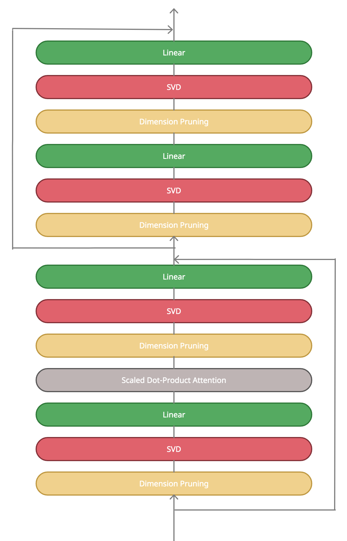
Figure 1. Further prune Vision Transformer via Singular Value Decomposition (SVD)

2.1. Vision Transformer (ViT)

The ViT model includes fully connected layer, Multi-Head Self-Attention(MHSA), linear transformer, Multi-Layer Perception, normalization layer, activation function, and shortcut connection.

2.1.1. Fully connected layer

: A fully connected layer is used to transform the input into characters that can be used in the next step, i.e. MHSA. Specifically, it can be denoted as:

$$I\rightarrow(Q_{I},K_{I},V_{I}).$$

The Input $I\in\mathbb{R}^{n\times d}$ is transformed to Query $Q\in\mathbb{R}^{n\times d}$, and Value $V\in\mathbb{R}^{n\times d}$ via fully-connected layers, where $n$ is the number of patches $d$ in the embedded dimension.

2.1.2. MHSA

: The self-attention mechanism is utilized to model the relationship between patches. It can be denoted as:

$$Attention(Q_{I},K_{I},V_{I})=Softmax\left(\frac{Q_{I}K_{I}^{T}}{\sqrt{d}}\right)V.$$

2.1.3. Linear Transformer

: A linear transformer is used to transform the output of MHSA. It can be denoted as:

$$Y=I+f_{out}(Attention(Q_{I},K_{I},V_{I})),$$

where the details of normalization layer and activation function are included in it.

2.1.4. Two-layer MLP

: Two feed forward MLP layers can be denoted as:

$$Z=Y+MLP_{2}(MLP_{1}(Y)).$$

2.2. Vision Transformer Pruning

The approach of Vision Transformer Pruning is to preserve the generated important features and remove the useless ones from the components of linear projection.

The pruning process is depending on the score of feature importance. We denote the matrix of feature importance scores is Diag$(a)\in\mathbb{R}^{n\times n}$, where $a\in\mathbb{R}^{d}$ represents each feature importance score. In order to enforce the sparsity of importance scores, we apply $l_{1}$ regularization on the importance scores $a$, which is denoted as $\hat{a}$, where $\hat{a}=\lambda||a||_{1}$ and $\lambda$ is the sparsity hyper-parameter. And optimize it by adding the training objective. We, therefore, obtain the transformer with some important scores near zero. We rank all the values of regularized importance scores in the transformer and obtain a threshold $\tau$ according to the predefined pruning rate. With the threshold, we obtain the discrete $a^{*}\in\mathbb{R}^{n\times n}$ score, which is denoted as

$$a^{*}=\left\{\begin{array}[]{rcrcrc@{\qquad}l}1&\text{ if }\hat{a}\geq\tau\\ 0&\text{ if }\hat{a}<\tau.\\ \end{array}\right.$$

The matrix $X$ after applying the pruning processes, denoted by

$$X^{*}=X\text{ Diag}(a^{*}),$$

and removing features with a zero score is transformed to $X^{*}\in\mathbb{R}^{r\times d}$. This pruning procedure is denoted as $\text{Prune}(X).$

2.3. Matrix Decomposition

We will introduce an experiential study of Matrix Decomposition methods particularly applied in our case. And a comparison of run-time complexity and the costs of those decomposition.

2.3.1. Eigenvalue Value Decomposition (EVD) of $X^{*}$

Note that a matrix has an EVD if and only if the matrix is diagonalizable. However, $X^{*}\in\mathbb{R}^{r\times d}$. When $r\neq d$, the $X^{*}$ has no EVD. So EVD has limitations while applying in our cases.

2.3.2. Singular Value Decomposition (SVD) of $X^{*}$

SVD is computed not depending on the dimension of the matrix. SVD can be applied to any matrix. Assume that $X^{*}\in\mathbb{R}^{m\times n}$ is the matrix after we have done the pruning procedure. Then $X^{*}$ has a decomposition that

$$X^{*}=U\Sigma V$$

where the left singular vectors $U\in\mathbb{R}^{m\times m}$ and right singular vectors $V\in\mathbb{R}^{n\times n}$ are both unitary matrices, which means $U^{*}U=I_{m}=UU^{*}$ and $V^{*}V=I_{n}=VV^{*}$. $\Sigma\in\mathbb{R}^{m\times n}$ is a diagonal matrix of $X^{*}$ in the sense that

$$\sigma_{ij}=\left\{\begin{array}[]{rcrcrc@{\qquad}l}0&\text{ if }i\neq j\\ \mathbb{R}_{+}&\text{ if }i=j\\ \end{array}\right.,$$

where the diagonal values are the set of singular values of the matrix $X^{*}$. This is the full SVD. We can also remove those singular values that are equal to zero from the matrix, which means $\sigma_{ii}=0$ for $i\in\text{max}\{m,n\}$. Then we get the form of $X^{*}$ that

$$X^{*}=U_{r}\Sigma_{r}V_{r},$$

where $U_{r}$, $\Sigma_{r}$, and $V_{r}$ $\in\mathbb{R}^{n\times n}$. This is the condensed SVD. $r$ is the rank of matrix $X^{*}$. The columns of $U_{r}$ forms an orthonormal basis for the image of $X^{*}$. The columns of $V_{r}$ forms an orthonormal basis for the coimage of $X^{*}$.

2.3.3. QR Decomposition of $X^{*}$

The QR decomposition method can solve many problems on the SVD list. The QR decomposition is cheaper to compute in the sense that there are direct algorithms for computing QR and complete orthogonal decomposition in a finite number of arithmetic steps. There are several versions of QR decomposition.

• Full QR Decomposition of $X^{*}$: For any matrix of $X^{*}\in\mathbb{R}^{m\times n}$, where $n\neq m$, there exits an unitary matrix $Q\in\mathbb{R}^{m\times m}$, $Q^{*}Q=QQ^{*}=I_{n}$ and an upper-triangular matrix $R\in\mathbb{R}^{m\times n}$, where $r_{ij}=0$ whenever $i>j$, such that

  $$X^{*}=QR=Q\begin{bmatrix}R_{1}\\ 0\end{bmatrix}.$$

  In which, $R_{1}\in\mathbb{R}^{n\times n}$ is an upper-triangular square matrix in general. If $X^{*}$ has full column rank, which is $rank(X^{*})=n$ then $R_{1}$ is non-singular.

• Reduced QR Decomposition of $X^{*}$: For any matrix of $X^{*}\in\mathbb{R}^{m\times n}$, where $n\neq m$, there exits an orthonormal matrix $Q\in\mathbb{R}^{m\times n}$, $Q^{*}_{1}Q_{1}=I_{n}$ but $Q_{1}Q^{*}_{1}\neq I_{m}$ unless $m=n$ and an upper-triangular square matrix $R\in\mathbb{R}^{n\times n}$, such that

  $$X^{*}=Q_{1}R_{1}.$$

  In which, $Q_{1}$ is the first $n$ columns of $Q$ in previous Full QR decomposition. $Q=[Q_{1},Q_{2}]$, where $Q_{2}\in\mathbb{R}^{m\times(m-n)}$ is the last $m-n$ columns of $Q$. In fact, we can obtain reduced QR decomposition of $X^{*}$ from the full QR decomposition of $X^{*}$ by simply multiplying out

  $$X^{*}=QR=[Q_{1},Q_{2}]\begin{bmatrix}R_{1}\\ 0\end{bmatrix}=Q_{1}R_{1}+Q_{2}0=Q_{1}R_{1}.$$

  If $X^{*}$ has full column rank, which means $rank(A)=n$, then $R_{1}$ is non-singular.

• Rank-Retaining QR Decomposition of $X^{*}$: For matrix of $X^{*}\in\mathbb{R}^{m\times n}$, where $rank(X^{*})=r$, there exists a permutation matrix $\Pi\in\mathbb{R}^{n\times n}$, a unitary matrix $Q\in\mathbb{R}^{m\times m}$, and a non-singular, upper-triangular square matrix $R_{1}\in\mathbb{R}^{r\times r}$, such that

  $$X^{*}\Pi=Q\begin{bmatrix}R_{1}&S\\ 0&0\end{bmatrix}.$$

  In which, $S\in\mathbb{R}^{r\times(n-r)}$ is just some matrix with no special properties. We can also write it as the form that

  $$X^{*}=QR\Pi^{T}=Q\begin{bmatrix}R_{1}&S\\ 0&0\end{bmatrix}\Pi^{T}.$$

• Complete Orthogonal Decomposition of $X^{*}$: For matrix of $X^{*}\in\mathbb{R}^{m\times n}$, where rank$(X^{*})=r$, there exists an unitary matrix $Q\in\mathbb{R}^{m\times m}$, an unitary matrix $U\in\mathbb{R}^{n\times n}$, and a non-singular, lower-triangular square matrix $L\in\mathbb{R}^{r\times r}$, such that

  $$X^{*}=Q\begin{bmatrix}L&0\\ 0&0\end{bmatrix}U^{*}.$$

  It can be obtained from a full QR decomposition of $\begin{bmatrix}R^{*}_{1}\\ S^{*}\end{bmatrix}\in\mathbb{R}^{m\times r}$, which has full column rank,

  $$\begin{bmatrix}R^{*}_{1}\\ S^{*}\end{bmatrix}=Z\begin{bmatrix}R_{2}\\ 0\end{bmatrix},$$

  where $Z\in\mathbb{R}^{m\times m}$ in unitary and $R_{2}\in\mathbb{R}^{r\times r}$ in non-singular, upper-triangular square matrix. Observe the Rank-Retaining QR Decomposition of $X^{*}$ that

  $$X^{*}=Q\begin{bmatrix}R_{1}&S\\ 0&0\end{bmatrix}\Pi^{T}=Q\begin{bmatrix}R_{2}^{*}&0\\ 0&0\end{bmatrix}Z*\Pi^{T}=Q\begin{bmatrix}L&0\\ 0&0\end{bmatrix}U^{*}.$$

2.3.4. LU Decomposition of $X^{*}$

For unstructured matrix $X^{*}$, the most common method is to obtain a decomposition $X^{*}=LU$, where $L$ is lower triangular and $U$ is upper triangular. LU decomposition is a sequence of constant LU decomposition. We are not just interested in the final upper triangular matrix, we are also interested in keeping track of all the elimination steps. We will omit this method, because it is intuitively expensive to storage and keep track of the complete L and U factors.

2.3.5. Cholesky Decomposition of $X^{*}$

The Cholesky Decomposition can be computed directly from the matrix equation $A=R^{T}R$ where $R$ is upper-triangular.

The matrix $X^{*}$ in our vision is dense, the Table 1 compares the relative merits of normal equations, QR decomposition, and SVD. By Table 1 and an experimental implementation. We finally selected SVD as the method to further prune Vision Transformer. As shown in Figure 1, we apply the SVD operation after each steps of Dimension Pruning operation, which is after pruning operation on all the MHSA and MLP blocks.

Merits	Evaluation
Accuracy	Normal Equation $<$ QR Decomposition $<$ SVD
Speed	Normal Equation $>$ QR Decomposition $>$ SVD

Table 1. A comparison of the relative merits among Normal Equations, QR Decomposition, and SVD.

3. Experimental Evaluation

In this section, we verify the effectiveness of the purposed methods to further prune the Vision Transformer via Matrix Decomposition on the CIFAR-10 dataset (Krizhevsky et al., 2010).

3.1. Dataset

The CIFAR-10 dataset (Krizhevsky et al., 2010) is divided into five training batches and one test batch, each with $10000$ images. The test batch contains exactly $1000$ randomly-selected images from each class. The training batches contain the remaining images in random order, but some training batches may contain more images from one class than another. Between them, the training batches contain exactly $5000$ images from each class.

3.1.1. CIFAR-10.

The CIFAR-10 is labeled subsets of the $80$ million tiny images dataset. They were collected by Alex Krizhevsky, Vinod Nair, and Geoffrey Hinton. The CIFAR-10 dataset consists of $60000$ images in $10$ classes, with $6000$ images per class. There are $50000$ training images and $10000$ test images.

3.2. Implementation Details

We modified the code book by adding Matrix Decomposition Methods we mentioned about into the places after doing the Vision Transformer Pruning operation. Since the code book is using the CIFAR$-10$, we do not modify other components of the code book. Figure 2 shows the result of those implementation. We will discuss it in the next section.

3.2.1. Baseline

We evaluate developed pruning method via matrix decomposition on a popular vision transformer implementation. In our experiments, a $12-$layer transformer with $10$ heads and $768$ embedding dimensions is evaluated on CIFAR$-10$. For a fair comparison, we utilize the official implementation of CIFAR$-10$. On the CIFAR$-10$, we take the released model of Vision Transformer Pruning as the baseline. We fine-tune the model on the CIFAR$-10$ using batch size $64$ for $30$ epochs. The initial learning rate is set to $6.25\times 10^{-7}$. Following Deit (Touvron et al., 2021), we use AdamW (Loshchilov and Hutter, 2018) with cosine learning rate decay strategy to train and fine-tune the models.

3.2.2. Training with Pruning

Based on the baseline model, we train the vision transformer with $l_{1}$ regularization using different sparse regularization rates. We select the optimal sparse regularization rate (i.e. $0.0001$) on CIFAR$-10$ and apply it on CIFAR$-10$. The learning rate for training with sparsity is $6.25\times 10-6$ and the number of epochs is $100$. The other training setting follows the baseline model. After sparsity, we prune the transformer by setting different pruning thresholds and the threshold is computed by the predefined pruning rate. Which is very similar with the original dataset.

3.2.3. Fine-tuning

We finetune the pruned transformer with the same optimization setting as in training, except for removing the $l_{1}$ regularization.

3.3. Results and Analysis

In Figure 2 shows a result of comparison of accuracy after implemented matrix decomposition methods, including SVD, QR decomposition, and LU decomposition. It is easy to see that the SVD performs pretty well comparing with the other two matrix decomposition methods including QR decomposition, and LU decomposition. By experience, the computation is not time consuming. The times of computation is nearly the same except the LU factorization. However, while comparing VTPSVD and VTP, the accuracy score of VTPSVD is not lower than the original VTP. which means that we need to further modify and develop our mathod to achieve a better performance in our case.

	VTP	VTPSVD	VTPQRD	VTPLUD
ViT patch=2	80%	85.0%	71.1%	63.7%
ViT patch=4	80%	62.8%	68.3%	57.1%
ViT patch=8	30%	53.2%	53.5%	52.3%
CIFAR-10	93%	53.2%	53.5%	49.2%

Table 2. A comparison of accuracy score among Vision Transformer Pruning (VTP), Vision Transformer Pruning with Singular Value Decomposition (VTPSVD), Vision Transformer Pruning with QR Decomposition (VTPQRD), and Vision Transformer Pruning with LU Decomposition (VTPLUD) with different patches.

4. Conclusion

In this paper, we build up on and further develop the method of Vision Transformer Pruning by adding a matrix decomposition operation to meet the same goal of reduce the storage, run-time memory, and computational demands. The experiments conducted on CIFAR-10 demonstrate that the pruning with Singular Value Decomposition method can largely reduce the computation costs and storage while maintaining a comparingly high accuracy with some patches. However, this method needs to be further develop to obtain a much robust optimal performance.

5. Future Work

There are several future works that I am planning to do:

• Test the method on other datasets, i.e. ImageNet (Russakovsky et al., 2015), which is the one used in the original Vision Transformer Pruning (Zhu et al., 2021b).

• Further develop and fine-tune this method.

References

- (1)
- Cai et al. (2017) Zhaowei Cai, Xiaodong He, Jian Sun, and Nuno Vasconcelos. 2017. Deep Learning with Low Precision by Half-wave Gaussian Quantization. arXiv:cs.CV/1702.00953
- Carion et al. (2020) Nicolas Carion, Francisco Massa, Gabriel Synnaeve, Nicolas Usunier, Alexander Kirillov, and Sergey Zagoruyko. 2020. End-to-End Object Detection with Transformers. arXiv:cs.CV/2005.12872
- Chen et al. (2021) Hanting Chen, Yunhe Wang, Tianyu Guo, Chang Xu, Yiping Deng, Zhenhua Liu, Siwei Ma, Chunjing Xu, Chao Xu, and Wen Gao. 2021. Pre-Trained Image Processing Transformer. arXiv:cs.CV/2012.00364
- Chen et al. (2020) Mark Chen, Alec Radford, Rewon Child, Jeffrey Wu, Heewoo Jun, David Luan, and Ilya Sutskever. 2020. Generative Pretraining From Pixels. , 1691–1703 pages.
- Cun et al. (1990) Yann Le Cun, John S. Denker, and Sara A. Solla. 1990. Optimal Brain Damage. , 598–605 pages.
- Denton et al. (2014) Emily Denton, Wojciech Zaremba, Joan Bruna, Yann LeCun, and Rob Fergus. 2014. Exploiting Linear Structure Within Convolutional Networks for Efficient Evaluation. arXiv:cs.CV/1404.0736
- Dosovitskiy et al. (2021) Alexey Dosovitskiy, Lucas Beyer, Alexander Kolesnikov, Dirk Weissenborn, Xiaohua Zhai, Thomas Unterthiner, Mostafa Dehghani, Matthias Minderer, Georg Heigold, Sylvain Gelly, Jakob Uszkoreit, and Neil Houlsby. 2021. An Image is Worth 16x16 Words: Transformers for Image Recognition at Scale.
- Guo et al. (2019) Qipeng Guo, Xipeng Qiu, Pengfei Liu, Yunfan Shao, Xiangyang Xue, and Zheng Zhang. 2019. Star-Transformer. arXiv:cs.CL/1902.09113
- Gupta et al. (2015) Suyog Gupta, Ankur Agrawal, Kailash Gopalakrishnan, and Pritish Narayanan. 2015. Deep Learning with Limited Numerical Precision. arXiv:cs.LG/1502.02551
- Han et al. (2021a) Kai Han, Yunhe Wang, Hanting Chen, Xinghao Chen, Jianyuan Guo, Zhenhua Liu, Yehui Tang, An Xiao, Chunjing Xu, Yixing Xu, Zhaohui Yang, Yiman Zhang, and Dacheng Tao. 2021a. A Survey on Vision Transformer. arXiv:cs.CV/2012.12556
- Han et al. (2021b) Kai Han, An Xiao, Enhua Wu, Jianyuan Guo, Chunjing Xu, and Yunhe Wang. 2021b. Transformer in Transformer. arXiv:cs.CV/2103.00112
- Hassibi and Stork (1992) Babak Hassibi and David Stork. 1992. Second order derivatives for network pruning: Optimal Brain Surgeon.
- Hu et al. (2021) Jie Hu, Liujuan Cao, Yao Lu, ShengChuan Zhang, Yan Wang, Ke Li, Feiyue Huang, Ling Shao, and Rongrong Ji. 2021. ISTR: End-to-End Instance Segmentation with Transformers. arXiv:cs.CV/2105.00637
- Krizhevsky et al. (2010) Alex Krizhevsky, Vinod Nair, and Geoffrey Hinton. 2010. Cifar-10. URL http://www. cs. toronto. edu/kriz/cifar. html 5 (2010), 4.
- Lee et al. (2019) Dongsoo Lee, Se Jung Kwon, Byeongwook Kim, and Gu-Yeon Wei. 2019. Learning Low-Rank Approximation for CNNs. arXiv:cs.LG/1905.10145
- Lin et al. (2019) Shaohui Lin, Rongrong Ji, Chao Chen, Dacheng Tao, and Jiebo Luo. 2019. Holistic CNN Compression via Low-Rank Decomposition with Knowledge Transfer. IEEE Transactions on Pattern Analysis and Machine Intelligence 41, 12 (2019), 2889–2905.
- Liu et al. (2017) Zhuang Liu, Jianguo Li, Zhiqiang Shen, Gao Huang, Shoumeng Yan, and Changshui Zhang. 2017. Learning Efficient Convolutional Networks through Network Slimming. arXiv:cs.CV/1708.06519
- Liu et al. (2021) Ze Liu, Yutong Lin, Yue Cao, Han Hu, Yixuan Wei, Zheng Zhang, Stephen Lin, and Baining Guo. 2021. Swin Transformer: Hierarchical Vision Transformer using Shifted Windows. arXiv:cs.CV/2103.14030
- Loshchilov and Hutter (2018) Ilya Loshchilov and Frank Hutter. 2018. Fixing Weight Decay Regularization in Adam. https://openreview.net/forum?id=rk6qdGgCZ
- Rastegari et al. (2016) Mohammad Rastegari, Vicente Ordonez, Joseph Redmon, and Ali Farhadi. 2016. XNOR-Net: ImageNet Classification Using Binary Convolutional Neural Networks. arXiv:cs.CV/1603.05279
- Russakovsky et al. (2015) Olga Russakovsky, Jia Deng, Hao Su, Jonathan Krause, Sanjeev Satheesh, Sean Ma, Zhiheng Huang, Andrej Karpathy, Aditya Khosla, Michael Bernstein, Alexander C. Berg, and Li Fei-Fei. 2015. ImageNet Large Scale Visual Recognition Challenge. arXiv:cs.CV/1409.0575
- Sun (2021) Tianyi Sun. 2021. How Personal Perceptions Of COVID-19 Have Changed Over Time.
- Sun and Gini (2021) Tianyi Sun and Maria Gini. 2021. Study of Natural Language Understanding. Journal of Chang Chun Teachers College 47 (2021).
- Sun and Nelson (2023) Tianyi Sun and Bradley Nelson. 2023. Topological Interpretations of GPT-3. arXiv:cs.CL/2308.03565
- Tai et al. (2016) Cheng Tai, Tong Xiao, Yi Zhang, Xiaogang Wang, and Weinan E. 2016. Convolutional neural networks with low-rank regularization. arXiv:cs.LG/1511.06067
- Tang et al. (2021) Yehui Tang, Yunhe Wang, Yixing Xu, Dacheng Tao, Chunjing Xu, Chao Xu, and Chang Xu. 2021. SCOP: Scientific Control for Reliable Neural Network Pruning. arXiv:cs.CV/2010.10732
- Tang et al. (2020) Yehui Tang, Shan You, Chang Xu, Jin Han, Chen Qian, Boxin Shi, Chao Xu, and Changshui Zhang. 2020. Reborn Filters: Pruning Convolutional Neural Networks with Limited Data. Proceedings of the AAAI Conference on Artificial Intelligence 34, 04 (2020), 5972–5980.
- Touvron et al. (2021) Hugo Touvron, Matthieu Cord, Matthijs Douze, Francisco Massa, Alexandre Sablayrolles, and Hervé Jégou. 2021. Training data-efficient image transformers & distillation through attention. arXiv:cs.CV/2012.12877
- Vaswani et al. (2017) Ashish Vaswani, Noam Shazeer, Niki Parmar, Jakob Uszkoreit, Llion Jones, Aidan N. Gomez, Lukasz Kaiser, and Illia Polosukhin. 2017. Attention Is All You Need. arXiv:cs.CL/1706.03762
- Wang et al. (2021c) Huiyu Wang, Yukun Zhu, Hartwig Adam, Alan Yuille, and Liang-Chieh Chen. 2021c. MaX-DeepLab: End-to-End Panoptic Segmentation with Mask Transformers. arXiv:cs.CV/2012.00759
- Wang et al. (2021a) Wenhai Wang, Enze Xie, Xiang Li, Deng-Ping Fan, Kaitao Song, Ding Liang, Tong Lu, Ping Luo, and Ling Shao. 2021a. Pyramid Vision Transformer: A Versatile Backbone for Dense Prediction without Convolutions. arXiv:cs.CV/2102.12122
- Wang et al. (2021b) Yuqing Wang, Zhaoliang Xu, Xinlong Wang, Chunhua Shen, Baoshan Cheng, Hao Shen, and Huaxia Xia. 2021b. End-to-End Video Instance Segmentation with Transformers. arXiv:cs.CV/2011.14503
- Wen et al. (2016) Wei Wen, Chunpeng Wu, Yandan Wang, Yiran Chen, and Hai Li. 2016. Learning Structured Sparsity in Deep Neural Networks. arXiv:cs.NE/1608.03665
- Yang et al. (2020) Zhaohui Yang, Yunhe Wang, Kai Han, Chunjing Xu, Chao Xu, Dacheng Tao, and Chang Xu. 2020. Searching for Low-Bit Weights in Quantized Neural Networks. arXiv:cs.CV/2009.08695
- Yu et al. (2017) Xiyu Yu, Tongliang Liu, Xinchao Wang, and Dacheng Tao. 2017. On compressing deep models by low rank and sparse decomposition. , 7370–7379 pages.
- Zhu et al. (2021b) Mingjian Zhu, Yehui Tang, and Kai Han. 2021b. Vision transformer pruning.
- Zhu et al. (2021a) Xizhou Zhu, Weijie Su, Lewei Lu, Bin Li, Xiaogang Wang, and Jifeng Dai. 2021a. Deformable DETR: Deformable Transformers for End-to-End Object Detection. arXiv:cs.CV/2010.04159