DynED: Dynamic Ensemble Diversification in Data Stream Classification

Abstract.

Ensemble methods are commonly used in classification due to their remarkable performance. Achieving high accuracy in a data stream environment is a challenging task considering disruptive changes in the data distribution, also known as concept drift. A greater diversity of ensemble components is known to enhance prediction accuracy in such settings. Despite the diversity of components within an ensemble, not all contribute as expected to its overall performance. This necessitates a method for selecting components that exhibit high performance and diversity. We present a novel ensemble construction and maintenance approach based on MMR (Maximal Marginal Relevance) that dynamically combines the diversity and prediction accuracy of components during the process of structuring an ensemble. The experimental results on both four real and 11 synthetic datasets demonstrate that the proposed approach (DynED) provides a higher average mean accuracy compared to the five state-of-the-art baselines.

1. INTRODUCTION

The ability to extract meaningful insights out of an endless flow of incoming data is crucial nowadays, and data stream classification methods have made this task more feasible. As more organizations move towards a more technology-driven environment, there has been an alarming increase in generated large amounts of real-time information coming from different sources, such as social media platforms, sensor-based systems, healthcare, etc. Data stream classification techniques offer rapid processing capabilities. This allows analysts to harness valuable insights at lightning speed. As a result, decision-making processes can be carried out promptly to minimize risks while improving performance.

Dealing with the dynamic nature of data streams is one of the main challenges with data stream classification due to changes in the data distribution. This phenomenon is known as concept drift (Tsymbal, 2004; Wang et al., 2011; Yuan et al., 2022; Gulcan and Can, 2023; Bakhshi et al., 2023), and necessitates a learning paradigm capable of handling it. Ensemble approaches combine multiple possibly weak classifiers to improve model performance, robustness, resilience distributivity, and redundancy (Vardi, 2020). These approaches have the ability to adapt to the changes in data distributions while maintaining high levels of accuracy (Wankhade et al., 2020; Wares et al., 2019; Bonab and Can, 2018).

The discrepancies in predictions provided by individual ensemble components are referred to as diversity. In the ensemble learning setting, maintaining diversity among the individual ensemble components is one of the main challenges. Exposure of the data stream environment to various concept drifts and the fast arrival rate of data items makes this challenge even harder. High-diversity ensembles demonstrate better performance in the presence of concept drift (Minku et al., 2010; Minku, 2011) even with fewer components (Bonab and Can, 2019). The performance of ensemble components can decrease drastically when concept drift occurs. To maintain high accuracy, it is critical to detect the concept drift and update or replace the impacted ensemble components (Minku, 2011).

Several approaches to handle the difficulties mentioned above have been proposed. Leveraging Bagging (LevBag) (Bifet et al., 2010a) combines bagging’s simplicity with additional randomization of component inputs and outputs. This randomization can help individual components in an ensemble make different predictions. Concerning diversity, the Adaptive Random Forest (ARF) (Gomes et al., 2017) uses a local randomization strategy to retain diversity among ensemble components. This method uses different random selections of features for each component in the ensemble, encouraging diversity among individual components.

Compared to the prior methods, the Streaming Random Patches (SRP) (Gomes et al., 2019) combines random subspaces and online bagging to achieve competitive prediction performance. As a result, they indirectly increase the diversity of the ensemble components. Lastly, Kappa Updated Ensemble (KUE) (Cano and Krawczyk, 2020) combines online and block-based methods and uses the Kappa statistic to weigh and select classifiers dynamically. To increase the diversity, each base learner is trained with a different subset of features. Additionally, new instances are added to each base learner with a specific probability based on the Poisson distribution.

The challenges of data stream classification and the efforts of the previous solutions to increase diversity within their ensembles have motivated further investigation. The aim is to determine how to add more variety and prune the redundant or ineffective components (Shen and Liu, 2021; Elbasi et al., 2021; Woźniak et al., 2023) in an ensemble to handle concept drift better, and maintain high accuracy.

The following are the main contributions of this research. We

• Propose a novel ensemble construction and maintenance approach, called DynED (Dynamic Ensemble Diversification), based on the principles of the Maximal Marginal Relevance (MMR) concept;

• Adjust the diversity parameter dynamically to cope with the data stream to have high diversity in case of severe drifts;

• Experiment with 15 datasets with varying drift types and compare our results with those of the state-of-the-art methods.

2. PROPOSED APPROACH

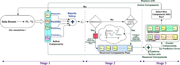
Figure 1. Ensemble construction and maintenance using DynED. Stage 1: Predicting, majority voting, and training. Stage 2: Detecting drifts, adding new components, and updating the diversity parameter. Stage 3: Selecting new components.

2.1. Using MMR in Data Stream Classification

Maximal Marginal Relevance (MMR) (Carbonell and Goldstein, 1998) is a diversity-based ranking method that minimizes redundancy while maintaining the relevance of a query in a document set. It is useful for text-document summarization, response extraction (Mao et al., 2020; Adams et al., 2022), and document re-ranking (Carbonell and Goldstein, 1998). Formally, the MMR method follows Eq. 1 to rank the documents:

(1) $$\footnotesize\text{MMR}=\operatorname*{argmax}_{D_{i}\in\texttt{R\textbackslash{}S}}[\lambda\times\text{sim}(D_{i},q)-(1-\lambda)\times\max_{D_{j}\in S}\text{sim}(D_{i},D_{j})]$$

In Eq.1, $D_{i}$ represents a document, $R$ is a ranked list of the documents, $S$ is a set of the selected documents, $\lambda$ is a parameter that balances accuracy and redundancy, and $sim(D_{i},q)$ measures the relevance between document $D_{i}$ and query $q$. When $\lambda=1$, MMR calculates the relevance-ranked list; when $\lambda=0$, it calculates a ranking that maximizes diversity among the documents in $R$. MMR optimizes a linear combination of relevance and diversity criteria for values of $\lambda$ between 0 and 1.

Table 1. Symbols & default hyperparameter values of DynED

Symbol	Meaning	Default value
$\xi_{slc}$	Set of selected components	—
$I$	Intensity of changes in the accuracy	—
$\theta$	Threshold for the count of processed samples	100
$\lambda$	Controlling parameter of similarity and accuracy	0.6
$\Delta_{\lambda}$	Variation in $\lambda$ parameter	0.1
$win_{s}$	Window size	500
$init_{c}$	Initial components count	5
$init_{s}$	Initial training sample size per component	50
$pool_{s}$	Maximum size of the component pool	500
$add_{s}$	# of components to add in each step	5
$cls_{s}$	# of components to select from each cluster	10
$slc_{s}$	# of active components for classification	10
$error_{s}$	Prediction list size to calculate similarity on	50
$cls_{slc}$	Set of selected components based on clustering	—
$cls_{rst}$	Set of not selected components based on clustering	—

It is necessary to make changes in its definition in order to adapt the MMR method for selecting and ranking ensemble components. In terms of ensemble components, the first part of Eq. 1, which calculates the relevance of $D_{i}$ to query $q$, is replaced with the accuracy of each component. It is represented as ”$\lambda\times\text{acc}(CS_{i},Ins)$”, where $\xi=\{CS_{1},CS_{2},...,CS_{m}\}$ is the set of ensemble classifiers, $CS_{i}$ represents each component, and $Ins$ are the previously seen instances of the data stream.

The second part of the Eq. 1 determines a pairwise similarity between the documents. However, evaluating the diversity of ensemble components is difficult since there is no commonly agreed-upon formal definition of diversity. Several methods are available for determining the pairwise diversity of classifiers in terms of correct/incorrect (oracle) outputs, such as Correlation Coefficient P (CP), double-fault measure (DF), Disagreement Measure (DM), and $Q$ statistic (Tsymbal et al., 2005; Kuncheva and Whitaker, 2001, 2003). To adapt the second part of the Eq. 1 to the context of component diversity, we replace it with the DF diversity measuring method (the procedure of diversity measure selection is explained in section 3.2). Therefore, the second part of the formal equation turns into ”$(1-\lambda)\times\max_{CS_{j}\in S}sim(CS_{i},CS_{j})$”. The final version of the MMR method for our task is presented in Eq. 2:

(2) $$\footnotesize\centering\text{MMR}=\operatorname*{argmax}_{CS_{i}\in\texttt{R\textbackslash{}S}}[\lambda\times\text{acc}(CS_{i},Ins)-(1-\lambda)\times\max_{CS_{j}\in S}sim(CS_{i},CS_{j})]\@add@centering$$

The MMR method utilizes a measure of similarity, which can be derived from the complement of a diversity measure.

2.2. Dynamic Ensemble Diversification: DynED

The working principles of our approach: DynED aims to dynamically ensure high accuracy by increasing diversity in the presence of concept drift and otherwise by decreasing it to reduce exposure to underperforming ensemble components. The pseudo-code for DynED is provided in Algorithms 1 and 2.

Algorithm 1 DynED: Main flow.

0: $D$: data stream, $W$: sliding window, $DD$: drift detector, $init_{s}$, $init_{c}$, $win_{s}$, $pool_{s}$, $error_{s}$, $add_{s}$, $\Delta_{\lambda}$

0: $\hat{y_{k}}$: prediction of each sample at time $t$

1: $\xi,\xi_{slc}\leftarrow\text{initialize }init_{c}\text{ components and train on }init_{s}\text{ samples}$

2: while $D$ has more samples do

3:    $\hat{y_{k}}\leftarrow\text{use selected components }\xi_{slc}\text{to predict using majority voting}$

4:    $W\leftarrow$ add sample to the sliding window

5:    $DD\leftarrow\text{update drift detector using correct/incorrect predictions}$

6:    train $\xi_{slc}$ on sample

7:    if $DD$ detects drift then

8:       $\xi\leftarrow$ generate and train $add_{s}$ new component on data in $W$, add to the pool

9:    end if

10:    if $\text{passed samples count}\geq\theta$ or new component is added then

11:       $I\leftarrow$ calculate the intensity of accuracy change to update the $\lambda$ parameter dynamically

12:       if $I\geq 0$ then

13:          increase $\lambda$ by $\Delta_{\lambda}$ until it reaches 1

14:       else

15:          decrease $\lambda$ by $\Delta_{\lambda}$ until it reaches 0

16:       end if

17:       $\xi_{slc}$, $\xi\leftarrow$ update $\xi_{slc}$ and $\xi$ using Algorithm 2

18:    end if

19: end while

Stage 1: The primary process includes predicting new samples and training selected components, which is outlined in Algorithm 1. As this method operates online, line 3 of Algorithm 1 uses selected components to predict new samples using Majority Voting (Leon et al., 2017; Dogan and Birant, 2019).
Stage 2: The Drift Detector, ADWIN (Bifet and Gavalda, 2007), is updated using the correct/incorrect predictions. If drift is detected, a new classifier is generated and trained on the last seen data available in the sliding window and then added to the reserved component pool $\xi$ (lines 5-9 of Algorithm 1). Suppose a new component is added or the processed sample count passes the $\theta$ threshold. In that case, the algorithm updates the $\lambda$ parameter to reflect the proper value of diversity based on the intensity of accuracy changes (lines 10-16). Then Algorithm 2 is called to update $\xi_{slc}$ and $\xi$. The intensity of changes in the accuracy is computed using the formula ”$acc(t)-acc(t-i)\mathbin{/}i$” where $acc(t)$ denotes the accuracy of the ensemble model at the t^th sample and $i$ is equivalent to $\theta$ in DynED.

Algorithm 2 DynED: Component selection.

0: $W$: data window, $\xi$, $\xi_{slc}$, $slc_{s}$, $\lambda$, $error_{s}$, $pool_{s}$, $cls_{s}$

0: $\xi$, $\xi_{slc}$

1: $P\leftarrow\text{ combine }\xi\text{ and }\xi_{slc}$ sorted by accuracy

2: while $len(p)\geq pool_{s}$ do

3:    remove the last component

4: end while

5: $PE\leftarrow$ obtain prediction error for all components recalling data from $W$

6: $cls\leftarrow$ cluster components based on $PE$ ”(two clusters)”

7: $cls_{slc}\leftarrow$ select $cls_{s}$ components from each cluster based on the accuracy

8: $cls_{rst}\leftarrow$ store rest of components

9: $\xi_{slc}$, $\xi_{rst}\leftarrow$ apply Eq. 2 on $cls_{slc}$ to obtain a new set of components to continue prediction

10: $\xi\leftarrow cls_{rst}+\xi_{rst}$

11: return  $\xi$, $\xi_{slc}$

Stage 3: Algorithm 2 selects a diverse set of components using an adapted MMR method presented in Eq. 2. The algorithm combines previously selected components with those in the reserve pool and maintains a fixed component count by sorting them based on accuracy and removing poorly performing components. In line 5 of Algorithm 2, prediction errors for all components on previous samples held in sliding window are obtained. In the following line, components are clustered using the K-means clustering algorithm (Hartigan and Wong, 1979) into two groups based on these prediction errors to apply the selection method effectively. After clustering, $cls_{s}$ high-performance components are selected from each cluster, resulting in a total of $2\times cls_{s}$ components out of $N$ where $N\leq pool_{s}$. In line 9 of Algorithm 2, an adapted MMR method is applied to perform the final selection step. This algorithm outputs a new set of selected components to predict new incoming samples of the stream actively and updates the reserved components pool as a result. The way an ensemble structure is constructed and maintained by DynED is illustrated in Figure 1.

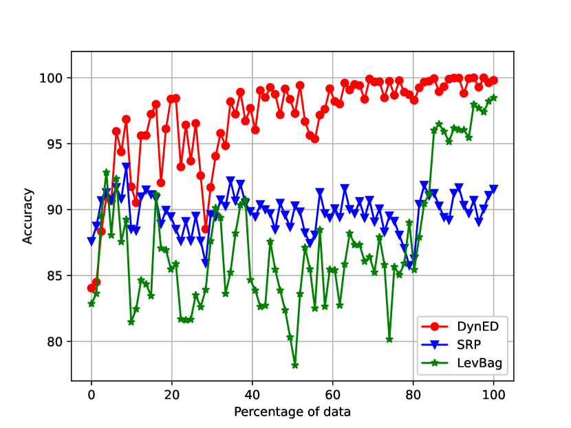
(a) Poker.

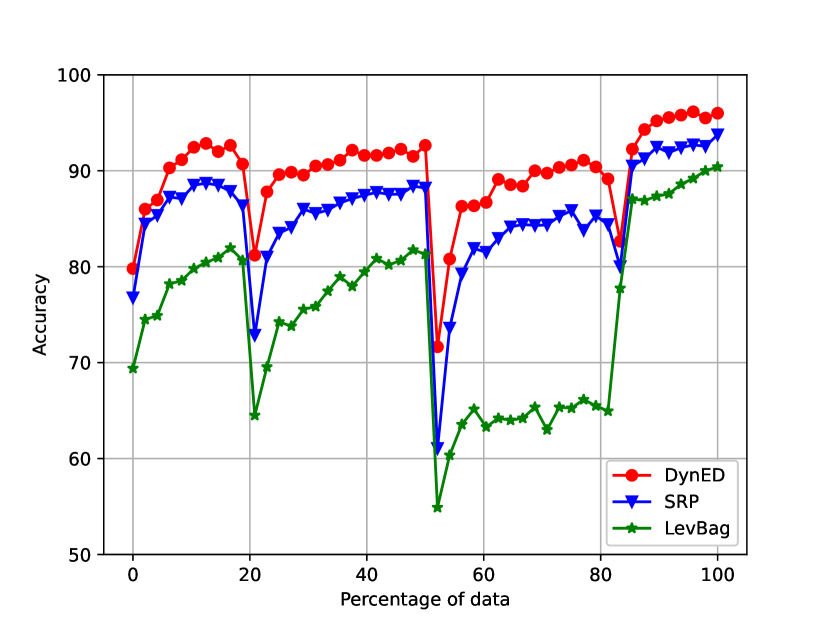
(b) Agrawal-4567.

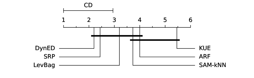
(c) Critical distance diagram.

Figure 2. (a, b): Prequential temporal accuracy results of DynED, and (c): Critical distance diagram, CD= 1.946.

Table 2. Characteristics of the datasets, average interleaved-test-then-train accuracy, and the rankings of the methods for each dataset. DT: Drift Type, —X—: No. of features, —y—: No. of classes, —$\mathcal{D}$—: No. of Samples

	Name	DT	—X—	—y—	—$\mathcal{D}$—	DynED	KUE	SRP	ARF	SAM-kNN	LevBag
Real	Electricity (Harries et al., 1999)	U	6	2	45,312	87.88	76.77	87.85	85.29	79.16	87.28
	Poker (Dua and Graff, 2017)	U	10	10	829,201	96.96	81.68	89.74	80.65	82.41	85.99
	Cover Types	U	54	7	581,012	94.66	84.30	94.07	90.06	93.87	90.94
	Weather (Elwell and Polikar, 2011)	U	8	2	18,152	78.17	72.74	78.79	78.28	78.24	77.87
Synthetic	Interchanging RBF (Losing et al., 2016a)	A	2	15	200,000	93.70	71.77	97.44	97.15	94.19	95.34
	LED-drift	A	7	10	100,000	99.99	95.33	99.32	96.65	99.94	99.96
	MG2C2D (Dyer et al., 2013)	I & G	2	2	200,000	92.68	93.17	94.53	94.49	94.52	94.54
	Moving Squares (Losing et al., 2016a)	I	2	4	200,000	85.02	30.05	86.95	56.95	97.34	87.77
	Rotating Hyperplane (Losing et al., 2016a)	I	10	2	200,000	84.69	83.36	85.79	81.53	86.25	86.05
	SEA-Abrupt-012	A & R	3	2	100,000	90.61	86.80	90.16	90.20	88.61	89.90
	SEA-Abrupt-123	A & R	3	2	100,000	90.10	86.60	89.79	89.61	88.43	89.60
	SEA-Gradual-012	G & R	3	2	100,000	80.33	77.28	79.83	79.77	77.20	79.76
	SEA-Gradual-123	G & R	3	2	100,000	80.30	77.56	79.82	79.57	76.93	79.60
	Agrawal-4567	G & I	9	2	100,000	89.95	75.41	84.29	73.64	73.91	74.77
	Mixed-12	A & R	4	2	100,000	98.47	89.45	93.44	97.02	98.20	94.71
	Average Mean	—	—	—	—	89.57	78.82	88.78	84.72	87.28	87.60
	Rank	—	—	—	—	2.20	5.46	2.44	4.00	3.73	3.20

2.3. Time Complexity Analysis of Component Selection

The time complexity of Algorithm 2, which employs the reformulated MMR method, is as follows. In line 5 of Algorithm 2, the prediction errors of all classifier components are obtained, the time complexity is $\mathcal{O}(p)$, where $p$ represents the classifier component count and $p\leq pool_{s}$. Lines 6, 7, and 8 of Algorithm 2 involve clustering the classifier components based on their prediction errors and selecting $cls_{s}$ from each cluster, where $cls_{s}<p$. The time complexity of these operations is $\mathcal{O}(k\times p\times itr)$, where $itr$ is the number of iterations in the clustering process, and $k$ is the number of clusters. $itr$ and $k$ are considered as constant as they are not hyperparameters for DynED. In line 10, which applies the reformulated MMR method, the time complexity can be broken down as follows: calculating the pairwise similarity of classifier components using any diversity measure has a time complexity of $\mathcal{O}(n^{2})$, where $n$ represents the number of classifier components extracted by the clustering step ($2\times cls_{s}$). Applying the reformulated MMR method itself has a time complexity of $\mathcal{O}(n\times j)$, where $j=slc_{s}$. Therefore, the overall time complexity of Algorithm 2 is $\mathcal{O}(p+k\times p\times itr+n\times j+n^{2})$. The dominant term in this time complexity analysis is $n^{2}$. Hence, the algorithm’s time complexity can be approximated as $\mathcal{O}(n^{2})$.

3. EXPERIMENTAL EVALUATION

3.1. Datasets

To assess the performance of our model, we conduct experiments using 15 datasets (Four real and 11 synthetic datasets) and compare them to the baseline models. The datasets cover a wide range of concept drift scenarios. Our experiments include all four types of drift: Gradual (G), Incremental (I), Abrupt (A), Recurring (R), and (U) stands for Unknown drift type. The synthetic datasets based on LED, SEA, Agrawal, and Mixed generators are created using the scikit-multiflow library (Montiel et al., 2018) and MOA framework (Bifet et al., 2010b). The LED dataset has seven drifting features without noise. The Agrawal dataset uses four classification functions, and the SEA dataset uses three classification functions to synthesize drift. The description of the datasets is shown in Table 2.2.

3.2. Setup

In our study, we evaluate four diversity measures: Correlation Coefficient P (CP), Double-Fault measure (DF), Disagreement Measure (DM), and $Q$ statistic. We apply each measure to Eq. 2 across all datasets to determine the most suitable diversity measure for DynED. Our results show that the DF has the highest average mean accuracy compared to that of CP, DM, and $Q$-statistic with respective average mean accuracies of 89.57, 88.14, 89.43, and 89.38. Therefore, we choose DF as the diversity measure in DynED.

We evaluate the performance of DynED against five state-of-the-art baselines including LevBag (Bifet et al., 2010a), SAM-kNN (Losing et al., 2016b), ARF (Gomes et al., 2017), and SRP (Gomes et al., 2019). These baselines are assessed using the Massive Online Analysis (MOA) (Bifet et al., 2010b) framework with default hyperparameters. For KUE (Cano and Krawczyk, 2020), we use the source code available on their GitHub for evaluation . DynED is implemented in Python 3.8 using the scikit-multiflow (Montiel et al., 2018) library, with a Hoeffding Tree as the base classifier, and split-confidence set to 9e-1 and grace-period set to 50. All baseline models were evaluated using the Interleaved-test-then-train approach. The codes and datasets for experiments are publicly available, and all experiments and results are reproducible .

The selection of appropriate hyperparameters is a critical aspect of all machine learning methods, including DynED. After conducting tests with various hyperparameters based on the grid search method, we determined the selected values presented in Table 1. These values serve as the default hyperparameters in DynED and are not tailored to any specific dataset. It should be noted that the first 250 samples of each dataset are used as a warm-up, and they are not involved in the accuracy calculations and final results presented in Table 2.2.

3.3. Results and Discussion

The overall accuracy of each method applied to each dataset is presented in Table 2.2, with the highest scores emphasized in bold. A comparative analysis reveals that DynED outperforms the baselines in 10 out of 15 datasets, particularly in three out of four real and seven out of 11 synthetic datasets. Furthermore, when the average mean accuracies are ranked in descending order, DynED emerges as the top performer with an average rank of 2.20. A closer examination of Table 2.2 and Figure 2.a and Figure 2.b indicates that DynED provides robustness in the case of gradual and recurrent drift types, outperforming the baselines in nearly all datasets that exhibit these drift types. However, DynED’s performance declines in the presence of incremental drift, struggling to maintain high accuracy levels throughout the stream. Nonetheless, when confronted with abrupt drifts, DynED effectively captures and addresses the drift by employing Eq. 2 to increase diversity among components, resulting in enhanced performance as evidenced by the plots in Figure 2. Overall, the results suggest that DynED is a promising method for the online classification of data streams. To assess the statistical significance of the employed methods, the Friedman Test is utilized in conjunction with the Nemenyi post-hoc analysis (Demšar, 2006). We calculate the Critical Distance as CD= 1.946. In our experiment, $\alpha=0.05$. The statistical test analysis, as presented in Figure 2.c, reveals that DynED statistically significantly outperforms KUE and achieves a better ranking among the other baseline methods.

4. CONCLUSION AND FUTURE WORK

This paper presents DynED, a novel ensemble construction and maintenance method that combines diversity and prediction accuracy for data stream classification tasks. It aims to increase the diversity among components in the presence of concept drift in a data stream in order to handle drifts better. The results show that DynED has higher average mean accuracy compared to the baseline models. In real-world scenarios, data stream environments often face the issue of label scarcity. As a part of future work, we aim to enhance our study for the semi-supervised classification of data streams.

5. ACKNOWLEDGMENTS

This study is partially supported by TÜBİTAK grant no. 122E271.

References

- (1)
- Adams et al. (2022) David Adams, Gandharv Suri, and Yllias Chali. 2022. Combining state-of-the-art models with maximal marginal relevance for few-shot and zero-shot multi-document summarization. arXiv (2022). https://doi.org/10.48550/arXiv.2211.10808
- Bakhshi et al. (2023) Sepehr Bakhshi, Pouya Ghahramanian, Hamed Bonab, and Fazli Can. 2023. A Broad ensemble learning system for drifting stream classification. IEEE Access (2023), 1–1. https://doi.org/10.1109/ACCESS.2023.3306957
- Bifet and Gavalda (2007) Albert Bifet and Ricard Gavalda. 2007. Learning from time-changing data with adaptive windowing. In Proceedings of the 2007 SIAM International Conference on Data Mining (SDM). SIAM, 443–448. https://doi.org/10.1137/1.9781611972771.42
- Bifet et al. (2010b) Albert Bifet, Geoff Holmes, Richard Kirkby, and Bernhard Pfahringer. 2010b. MOA: Massive online analysis. The Journal of Machine Learning Research 11 (2010), 1601–1604. https://doi.org/10.5555/1756006.1859903
- Bifet et al. (2010a) Albert Bifet, Geoff Holmes, and Bernhard Pfahringer. 2010a. Leveraging bagging for evolving data streams. In Machine Learning and Knowledge Discovery in Databases: European Conference, ECML PKDD 2010, Barcelona, Spain, September 20-24, 2010, Proceedings, Part I 21. Springer, 135–150. https://doi.org/10.1007/978-3-642-15880-3_15
- Bonab and Can (2019) Hamed Bonab and Fazli Can. 2019. Less Is More: A Comprehensive framework for the number of components of ensemble classifiers. IEEE Transactions on Neural Networks and Learning Systems 30, 9 (2019), 2735–2745. https://doi.org/10.1109/TNNLS.2018.2886341
- Bonab and Can (2018) Hamed R Bonab and Fazli Can. 2018. GOOWE: Geometrically optimum and online-weighted ensemble classifier for evolving data streams. ACM Transactions on Knowledge Discovery from Data (TKDD) 12, 2 (2018), 1–33. https://doi.org/10.1145/3139240
- Cano and Krawczyk (2020) Alberto Cano and Bartosz Krawczyk. 2020. Kappa updated ensemble for drifting data stream mining. Machine Learning 109 (2020), 175–218. https://doi.org/10.1007/s10994-019-05840-z
- Carbonell and Goldstein (1998) Jaime Carbonell and Jade Goldstein. 1998. The use of MMR, diversity-based reranking for reordering documents and producing summaries. In Proceedings of the 21st annual international ACM SIGIR conference on Research and development in information retrieval. 335–336. https://doi.org/10.1145/290941.291025
- Demšar (2006) Janez Demšar. 2006. Statistical comparisons of classifiers over multiple data sets. The Journal of Machine Learning Research 7 (2006), 1–30.
- Dogan and Birant (2019) Alican Dogan and Derya Birant. 2019. A Weighted majority voting ensemble approach for classification. In 2019 4th International Conference on Computer Science and Engineering (UBMK). 1–6. https://doi.org/10.1109/UBMK.2019.8907028
- Dua and Graff (2017) Dheeru Dua and Casey Graff. 2017. UCI Machine Learning Repository. http://archive.ics.uci.edu/ml
- Dyer et al. (2013) Karl B Dyer, Robert Capo, and Robi Polikar. 2013. Compose: A Semisupervised learning framework for initially labeled nonstationary streaming data. IEEE Transactions on Neural Networks and Learning Systems 25, 1 (2013), 12–26. https://doi.org/10.1109/TNNLS.2013.2277712
- Elbasi et al. (2021) Sanem Elbasi, Alican Büyükçakır, Hamed Bonab, and Fazli Can. 2021. On-the-Fly ensemble pruning in evolving data streams. https://doi.org/10.48550/arXiv.2109.07611 arXiv:2109.07611 [cs.LG]
- Elwell and Polikar (2011) Ryan Elwell and Robi Polikar. 2011. Incremental learning of concept drift in nonstationary environments. IEEE Transactions on Neural Networks 22, 10 (2011), 1517–1531. https://doi.org/10.1109/TNN.2011.2160459
- Gomes et al. (2017) Heitor M Gomes, Albert Bifet, Jesse Read, Jean Paul Barddal, Fabrício Enembreck, Bernhard Pfharinger, Geoff Holmes, and Talel Abdessalem. 2017. Adaptive random forests for evolving data stream classification. Machine Learning 106 (2017), 1469–1495. https://doi.org/10.1007/s10994-017-5642-8
- Gomes et al. (2019) Heitor Murilo Gomes, Jesse Read, and Albert Bifet. 2019. Streaming random patches for evolving data stream classification. In 2019 IEEE International Conference on Data Mining (ICDM). IEEE, 240–249. https://doi.org/10.1109/ICDM.2019.00034
- Gulcan and Can (2023) Ege Berkay Gulcan and Fazli Can. 2023. Unsupervised concept drift detection for multi-label data streams. Artificial Intelligence Review 56, 3 (2023), 2401–2434. https://doi.org/10.1007/s10462-022-10232-2
- Harries et al. (1999) Michael Harries, New South Wales, et al. 1999. Splice-2 comparative evaluation: Electricity pricing. (1999).
- Hartigan and Wong (1979) John A Hartigan and Manchek A Wong. 1979. Algorithm AS 136: A k-means clustering algorithm. Journal of the Royal Statistical Society Series C (Applied Statistics) 28, 1 (1979), 100–108. https://doi.org/10.2307/2346830
- Kuncheva and Whitaker (2001) Ludmila I Kuncheva and Chris J Whitaker. 2001. Ten measures of diversity in classifier ensembles: Limits for two classifiers. In A DERA/IEE Workshop on Intelligent Sensor Processing (Ref. No. 2001/050). IET, 10–1. https://doi.org/c10.1049/ic:20010105
- Kuncheva and Whitaker (2003) Ludmila I Kuncheva and Christopher J Whitaker. 2003. Measures of diversity in classifier ensembles and their relationship with the ensemble accuracy. Machine learning 51, 2 (2003), 181. https://doi.org/10.1023/A:1022859003006
- Leon et al. (2017) Florin Leon, Sabina-Adriana Floria, and Costin Bădică. 2017. Evaluating the effect of voting methods on ensemble-based classification. In 2017 IEEE International Conference on INnovations in Intelligent SysTems and Applications (INISTA). 1–6. https://doi.org/10.1109/INISTA.2017.8001122
- Losing et al. (2016a) Viktor Losing, Barbara Hammer, and Heiko Wersing. 2016a. KNN Classifier with self adjusting memory for heterogeneous concept drift. In 2016 IEEE 16th International Conference on Data Mining (ICDM). 291–300. https://doi.org/10.1109/ICDM.2016.0040
- Losing et al. (2016b) Viktor Losing, Barbara Hammer, and Heiko Wersing. 2016b. KNN classifier with self adjusting memory for heterogeneous concept drift. In 2016 IEEE 16th International Conference on Data Mining (ICDM). IEEE, 291–300. https://doi.org/10.1109/ICDM.2016.0040
- Mao et al. (2020) Yuning Mao, Yanru Qu, Yiqing Xie, Xiang Ren, and Jiawei Han. 2020. Multi-document summarization with maximal marginal relevance-guided reinforcement learning. In Proceedings of the 2020 Conference on Empirical Methods in Natural Language Processing (EMNLP). Association for Computational Linguistics, Online, 1737–1751. https://doi.org/10.18653/v1/2020.emnlp-main.136
- Minku (2011) Leandro Lei Minku. 2011. Online ensemble learning in the presence of concept drift. Ph. D. Dissertation. University of Birmingham.
- Minku et al. (2010) Leandro L. Minku, Allan P. White, and Xin Yao. 2010. The Impact of diversity on online ensemble learning in the presence of concept Drift. IEEE Transactions on Knowledge and Data Engineering 22, 5 (2010), 730–742. https://doi.org/10.1109/TKDE.2009.156
- Montiel et al. (2018) Jacob Montiel, Jesse Read, Albert Bifet, and Talel Abdessalem. 2018. Scikit-multiflow: A multi-output streaming framework. The Journal of Machine Learning Research 19, 1 (2018), 2915–2914.
- Shen and Liu (2021) Zixiong Shen and Xingcheng Liu. 2021. A New ensemble pruning method based on margin and diversity. In Mobile Multimedia Communications, Jinbo Xiong, Shaoen Wu, Changgen Peng, and Youliang Tian (Eds.). Springer International Publishing, Cham, 689–701. https://doi.org/10.1007/978-3-030-89814-4_50
- Tsymbal (2004) Alexey Tsymbal. 2004. The problem of concept drift: Definitions and related work. Computer Science Department, Trinity College Dublin 106, 2 (2004), 58. https://api.semanticscholar.org/CorpusID:8335940
- Tsymbal et al. (2005) Alexey Tsymbal, Mykola Pechenizkiy, and Pádraig Cunningham. 2005. Diversity in search strategies for ensemble feature selection. Information Fusion 6, 1 (2005), 83–98. https://doi.org/10.1016/j.inffus.2004.04.003
- Vardi (2020) Moshe Y Vardi. 2020. Efficiency vs. resilience: What COVID-19 teaches computing. , 9–9 pages. https://doi.org/10.1145/3388890
- Wang et al. (2011) Shenghui Wang, Stefan Schlobach, and Michel Klein. 2011. Concept drift and how to identify it. Journal of Web Semantics 9, 3 (2011), 247–265. https://doi.org/10.1016/j.websem.2011.05.003 Semantic Web Dynamics Semantic Web Challenge, 2010.
- Wankhade et al. (2020) Kapil K Wankhade, Snehlata S Dongre, and Kalpana C Jondhale. 2020. Data stream classification: A review. Iran Journal of Computer Science 3 (2020), 239–260. https://doi.org/10.1007/s42044-020-00061-3
- Wares et al. (2019) Scott Wares, John Isaacs, and Eyad Elyan. 2019. Data stream mining: Methods and challenges for handling concept drift. SN Applied Sciences 1 (2019), 1–19. https://doi.org/10.1007/s42452-019-1433-0
- Woźniak et al. (2023) Michał Woźniak, Paweł Zyblewski, and Paweł Ksieniewicz. 2023. Active weighted aging ensemble for drifted data stream classification. Information Sciences 630 (2023), 286–304. https://doi.org/10.1016/j.ins.2023.02.046
- Yuan et al. (2022) Liheng Yuan, Heng Li, Beihao Xia, Cuiying Gao, Mingyue Liu, Wei Yuan, and Xinge You. 2022. Recent advances in concept drift adaptation methods for deep learning. In Proceedings of the Thirty-First International Joint Conference on Artificial Intelligence, IJCAI-22, Lud De Raedt (Ed.). International Joint Conferences on Artificial Intelligence Organization, 5654–5661. https://doi.org/10.24963/ijcai.2022/788 Survey Track.