Differentiable Frank-Wolfe Optimization Layer

Abstract

Differentiable optimization has received a significant amount of attention due to its foundational role in the domain of machine learning based on neural networks. The existing methods leverages the optimality conditions and implicit function theorem to obtain the Jacobian matrix of the output, which increases the computational cost and limits the application of differentiable optimization. In addition, some non-differentiable constraints lead to more challenges when using prior differentiable optimization layers. This paper proposes a differentiable layer, named Differentiable Frank-Wolfe Layer (DFWLayer), by rolling out the Frank-Wolfe method, a well-known optimization algorithm which can solve constrained optimization problems without projections and Hessian matrix computations, thus leading to a efficient way of dealing with large-scale problems. Theoretically, we establish a bound on the suboptimality gap of the DFWLayer in the context of $\ell_{1}$-norm constraints. Experimental assessments demonstrate that the DFWLayer not only attains competitive accuracy in solutions and gradients but also consistently adheres to constraints. Moreover, it surpasses the baselines in both forward and backward computational speeds.

1 Introduction

Recent years have witnessed a variety of combining neural networks and conventional optimization as differentiable optimization layers to integrate expert knowledge into machine learning systems. With objectives and constraints deriving from that knowledge, the output of each differentiable optimization layer is the solution to a specific optimization problem whose parameters are outputs from previous layers (Amos and Kolter 2017; Agrawal et al. 2019; Sun et al. 2022; Landry 2021). Nevertheless, adapting the implicit functions (mapping parameters to solutions) to the training procedure of deep learning architecture is not easy since the explicit differentiable closed-form solutions are not available for most conventional optimization algorithms.

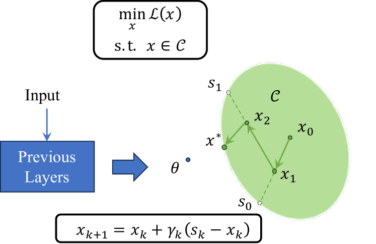
Figure 1: Illustration of DFWLayer. The simple convex combination ($0\leq\gamma_{k}\leq 1$) guarantees that each iteration is in the feasible region, and enables automatic differentiation.

On top of directly obtaining differentiable closed-form solutions, one alternative is to recover gradients respect to some parameters after solving for the optimal solution (Landry 2021). Two main categories of recovering gradients for optimal solutions have emerged: differentiating the optimality conditions and rolling out solvers. Differentiating the optimality conditions, namely the Karush–Kuhn–Tucker (KKT) conditions, seeks to differentiate a set of necessary conditions for a solution in nonlinear programming to be optimal, and has been effectively used in notable areas, such as bilevel optimization (Ghadimi and Wang 2018) and sensitivity analysis (Stechlinski, Khan, and Barton 2018). By leveraging these conditions and implicit function theorem, this approach is able to compute the Jacobian matrix and, thus, recover the gradients of optimal solutions (Amos and Kolter 2017; Agrawal et al. 2019). However, differentiating the KKT conditions directly might not always be computationally feasible or efficient, particularly for large-scale problems. Rolling out solvers is an unrolling method using iterative optimization algorithms as a series of trainable modules. By rolling out each iterative step of the optimization solver, the framework can backpropagate through the entire sequence, enabling direct training of these modules (Donti, Rolnick, and Kolter 2020). However, the rolling-out solvers might not converge or take a very long time to converge, which can lead to suboptimal solutions and impact the overall performance of the system (Bambade et al. 2023). Moreover, some methods based on alternating direction method of multipliers (ADMM) involve Hessian matrix computations, which can be computationally expensive, to recover gradients (Sun et al. 2022).

As for forward pass, a simple idea is to augment original training loss function with regularization terms regarding each constraints so that neural networks obtain the ability to infer feasible solutions. However, the feasibility is not guaranteed especially when encountering Out-of-Distribution (OOD) data. For a more robust solution, one might consider projection-based layers. Rather than attempting to incorporate constraints within the loss function itself, these layers operate by projecting each intermediate solution back onto the feasible region defined by the constraints during the optimization process (Amos and Kolter 2017; Agrawal et al. 2019). This can provide a more reliable adherence to constraints even in the presence of OOD data, increasing the robustness and reliability of the model. Nonetheless, this approach comes with the increasing computational cost associated with the projection step and the problem size. Thus, while projection-based layers can enhance the reliability of constraint satisfaction, their computational cost can be a significant trade-off that needs to be considered (Kasaura et al. 2023). Meanwhile, unrolling methods are not reliable without projections for constrained optimization problems, although they are easy to implement. Some methods use sufficient pre-training or positive slack variables to avoid projections, however, leading to unstable feasibility (Donti, Rolnick, and Kolter 2020; Sun et al. 2022).

In addition, the presence of non-differentiable constraints can pose significant challenges to differentiable optimization. In essence, existing differentiable optimization layers rely on the differentiability to construct the optimality conditions or the iterative solutions. Nevertheless, constraints in the real-world tasks are commonly non-differentiable, such as power constraints in robotics (Lin et al. 2021; Kasaura et al. 2023) and difference constraints in total variation denoising (Amos and Kolter 2017; Yeh et al. 2022).

In this paper, we aim to propose a differentiable optimization layer which accelerates both the optimization and backprogation procedure with non-differentiable norm constraints. Inspired by the Frank-Wolfe algorithms (also called the conditional gradient algorithms), we developed a framework, named Differentiable Frank-Wolfe Layer (DFWLayer), to efficiently deal with non-differentiable constraints which are expensive to project onto corresponding feasible region. As presented in Figure 1, DFWLayer first utilizes linear approximation for the original objective and find optimal solutions over the vertices of the feasible region. Then gradients computation is implemented with probabilistic approximation in each iterative step. Therefore, based on first-order optimization methods, DFWLayer omits high computational expense of projection and Hessian matrix computations, and thus speeds up solutions inference and gradients computation especially when encountering hard-to-project non-differentiable norm constraints. The proposed method can be highlighted as follows:

• We develop a new differentiable optimization layer which accelerates both the optimization and backprogation procedure with non-differentiable norm constraints. DFWLayer is based on first-order optimization methods which avoid projections and Hessian matrix computations, thus leading to efficient inference and gradients computation.

• We give theoretical analysis of the suboptimality gap for DFWLayer which depends on the smoothness of the objective, the diameter of the feasible region and the Maximum Mean Discrepancy (MMD) between the approximating distribution and the target distribution. The theorem is used to design a annealing temperature to enhance the accuracy and stabilize the gradients computation of DFWLayer.

• We conduct several experiments and validates that DFWLayer achieves competitive performance compared to state-of-the-art methods with acceptable margin of accuracy in an efficient way.

2 Related work

Differentiating the optimality conditions.

Differentiating the optimality conditions, namely the KKT conditions, leverages a set of necessary conditions for optimal solutions. OptNet (Amos and Kolter 2017) and CvxpyLayer (Agrawal et al. 2019) are typical differentiable optimization layers which recover gradients based on differentiation the KKT conditions. OptNet (Amos and Kolter 2017) solves quadratic programs based on prime-dual interior point method in the forward pass, while CvxpyLayer (Agrawal et al. 2019) requires calling a solver, such as open-source solvers SCS (O’Donoghue 2021) and ECOS (Domahidi, Chu, and Boyd 2013), to cope with more general convex optimization programs by casting them as cone programs. Then both layers differentiate the optimality conditions of convex optimization (Optnet can only handle quadratic programs) and compute the gradients of solution with implicit function theorem, which can be computationally expensive for large-scale problems.

Rolling out solvers.

Rolling out solvers is an alternative to conduct differentiable optimization. The optimization process can be automatically or manually unrolled, enabling the acquisition of derivatives during training (Landry 2021). Crucially, these derivatives take into account the effects of the embedded, or ‘in-the-loop’, optimization procedures. Alt-Diff (Sun et al. 2022) decouples the constrained optimization problem into multiple subproblems where the subproblem for prime variable is unconstrained and the solutions for dual variables are unrolled iteratively, thus decreasing the dimension of the Jacobian matrix. DC3 (Donti, Rolnick, and Kolter 2020) implicitly completes partial solutions to enforce equality constraints and unrolls gradient-based corrections to satisfy inequality constraints. Although these methods attempt to improve the reliability with some techniques (sufficient pre-training or positive slack variables), they always have the probability to violate constraints.

Differentiable projection.

Some simple differentiable projection layers have already been Incorporated in neural networks to integrate specialized kinds of constraints, such as softmax, sigmoid, ReLU and convolutional layers (Amos 2019; Donti, Rolnick, and Kolter 2020). For more general constraints, $\alpha$-projection (Sanket et al. 2020) and radial squashing (Kasaura et al. 2023) map inputs to some feasible solutions through an interior point. While these two layers are effective in some scenarios, they require to compute an interior point, such that, for any point in the feasible region, the segment between it and the interior point is contained in the feasible region, such as the Chebyshev center for linear constraints. For general constraints, computing the interior point is not always computationally feasible.

3 Preliminary

We consider a parameterized convex optimization problem with norm constraints:

$$\min_{x}f(x;\theta)\ \ \ \ \text{s.t.}\ x\in\mathcal{C}(\theta),$$ (1)

where $f:\mathbb{R}^{n}\rightarrow\mathbb{R}$ is convex and $L$-smooth, and $\mathcal{C}(\theta)$ is the convex feasible region; $x\in\mathbb{R}^{n}$ is the decision variable, and $\theta\in\mathbb{R}^{m}$ are the parameters of the optimization problem. The problem (1) aims to find the solution $x^{\ast}(\theta)$ in the feasible region $\mathcal{C}(\theta)$ with respect to the parameters $\theta$.

Differentiable Optimization Layers

In order to further illustrate optimization layers, we classify the parameters as dependent and independent ones, $\theta=\{\theta^{\rm d},\theta^{\rm ind}\}$. Since the optimization problem (1) can be viewed as an implicit function mapping from the parameters $\theta$ to the solution $x^{\ast}$, it can also be regarded as a layer, namely optimization layer (Sun et al. 2022), in neural networks with $\theta^{\rm d}$ being its input and $x^{\ast}$ being its output. Furthermore, optimization layer can be divided into two types according to whether $\theta^{\rm ind}$ are learnable or not.

Definition 3.1 (Fixed Optimization Layer).

An optimization layer is defined as a fixed optimization layer if some of its parameters are dependent on its input, while the others are fixed during training phase.

For most real-world tasks, Fixed Optimization Layer is a practical and effective choice with objectives and constraints embedded from expert knowledge. The independent parameters are fixed for some specific physical laws or physical constraints, such as Kirchhoff’s laws (Donti, Rolnick, and Kolter 2020; Chen et al. 2021), rigid body motion limitations and source power limitations (Kasaura et al. 2023). However, for some domain where we don’t have clear expert knowledge, Learnable Optimization Layer might achieve a good performance.

Definition 3.2 (Learnable Optimization Layer).

An optimization layer is defined as a Learnable optimization layer if some of its parameters are dependent on its input, while the others are learnable during training phase.

Learnable Optimization Layer is a type of optimization layers with randomly initialized independent parameters $\theta^{\rm ind}$ updated like other layers in the neural networks. Amos and Kolter (2017) conducted some experiments to learn independent parameters (without any information from the input), and to ensure a feasible solution always exist. Although Learnable OptNet (also called Pure OptNet in the original paper) seems to learn the similar difference operator with that used by total variation denoising, the accuracy is substantially low. Therefore, we will focus on fixed optimization layer and try to integrate domain-specific knowledge into optimization layers, and dependent parameters are denoted as $\theta$ for simplicity.

For such an optimization layer to be useful in machine learning system, the derivatives should be obtained with explicit or implicit functions, $x^{\ast}(\theta)$. If the Jacobian matrix can be computed, we can obtain the gradients of the loss with respect to the parameters given a loss function $\mathcal{L}$:

$$\frac{\partial\mathcal{L}}{\partial\theta}=\frac{\partial\mathcal{L}}{\partial x^{\ast}(\theta)}\frac{\partial x^{\ast}(\theta)}{\partial\theta}.$$ (2)

Then, the objective function in problem (1) is commonly defined as $f(x;\theta)=\frac{1}{2}\lVert x-\theta\rVert^{2}$ for optimization layers, with $\theta$ inferred by previous layers, whose parameters $\phi$ are updated by $\frac{\partial\mathcal{L}}{\partial\phi}=\frac{\partial\mathcal{L}}{\partial\theta}\frac{\partial\theta}{\partial\phi}$.

Conditional Gradient Methods

The conditional gradient methods, also known as the Frank-Wolfe algorithms, are a set of iterative optimization algorithm used for minimizing a differentiable convex function over a compact convex set (Braun et al. 2022). The methods are especially beneficial when dealing with complex or high-dimensional feasible sets, and are commonly compared with the projected gradient methods.

The projected gradient methods solve problem (1) with projection after each step of gradient descent, however, projection operations onto the norm ball are relatively computationally expensive and difficult except for some special cases such as $\ell_{1},\ell_{2},\ell_{\infty}$-norm. By contrast, the Frank-Wolfe methods can efficiently address the problem with tractable linear optimization over the feasible set.

Algorithm 1 Vanilla Frank-Wolfe (Frank, Wolfe et al. 1956)

1:  Let $x_{0}\in\mathcal{C}$.

2:  for $k=0,...,K$ do

3:     Compute $s_{k}\in\arg\min_{s\in\mathcal{C}}\langle\ \nabla_{x}f(x_{k}),s\rangle$.

4:     Update $x_{k+1}=(1-\gamma_{k})x_{k}+\gamma_{k}s_{k}$, for $\gamma_{k}=\frac{2}{k+2}$.

5:  end for

For the convergence analysis, based on the suboptimality gap $h(x_{k})=f(x_{k})-f(x^{\ast})$, Algorithm 1 matches the sublinear rate for projected gradient descent. With the domain diameter $M$ defined by $M=\sup_{x,y\in\mathcal{C}}\lVert x-y\rVert$, the suboptimality gap for Algorithm 1 is bounded by $O(\frac{1}{k})$, namely $h(x_{k})\leq\frac{2LM^{2}}{k+2}$ (Braun et al. 2022).

4 Differentiable Frank-Wolfe Layer

In this section, the details of DFWLayer are introduced by answering two questions: how does DFWLayer infer the optimal solution efficiently and how does DFWLayer compute the gradients respect to the parameters. For simplicity, we focus on cases with non-differentiable norm constraints which are general in real-world tasks. We consider such an optimization problem specifying problem (1) with norm constraints:

$$\min_{x}f(x;\theta)\ \ \ \ \text{s.t.}\ \lVert w\circ x\rVert\leq t,$$ (3)

where $w\in\mathbb{R}^{n}$ is a weight vector, and $t\in\mathbb{R}^{+}$ is a non-negative constant, and $\circ$ denotes the Hadamard production.

Forward Pass

Similar with Vanilla Frank-Wolfe (line 3 in Algorithm 1), the linear approximation of the original objective problem (3) is optimized with speciallized norm constraints:

$$s_{k} \in\arg\min_{s\in\mathcal{C}}\langle\ \nabla_{x}f(x_{k}),s\rangle$$

$$=\arg\min_{\lVert w\circ s\rVert\leq t}\langle\ \nabla_{x}f(x_{k}),s\rangle$$

$$=-\frac{t}{w}\circ\big{(}\arg\max_{\lVert s’\rVert\leq 1}\langle\ \frac{t}{w}\circ\nabla_{x}f(x_{k}),s’\rangle\big{)}$$

$$=-\frac{t}{w}\circ\partial\lVert g_{tw}(x_{k})\rVert_{\ast},$$ (4)

where $g_{tw}(\cdot)=\frac{t}{w}\circ\nabla_{x}f(\cdot)$, and $\lVert\cdot\rVert_{\ast}$ denotes the corresponding dual norm, $\partial\lVert\cdot\rVert_{\ast}$ denotes the subgradients of the dual norm, and $\frac{1}{w}$ denotes the element-wise division.

Given the widespread use of $\ell_{p}$-norm constraints in various applications, we considering $\ell_{p}$-norm constraints, $\lVert w\circ x\rVert_{p}\leq t$, and the subgradients of $\ell_{p}$-norm for further study so that (4) can be derived as

$$s_{k,i}=-\frac{\alpha t}{w}\cdot{\rm sign}(g_{tw,i}(x_{k}))\cdot\lvert g_{tw,i}(x_{k})\rvert^{\frac{p}{q}},$$ (5)

where $i=1,...,n$ stands for the $i^{\rm th}$ entry of the vector, and $q$ is a positive constant such that $\frac{1}{p}+\frac{1}{q}=1$, and $\alpha$ is a constant such that $\lVert s_{k}\rVert_{q}=1$. It is noted that, when $p>1$, $\lVert\cdot\rVert_{p}$ is differentiable such that subgradients equal to gradients uniquely. When $p=1$, a more practical expression of vertex other than (5) is

$$s_{k}=-\frac{t}{w}\circ{\rm sign}(g_{tw,i}(x_{k}))\circ e_{i_{k}},$$ (6)

where $e_{i_{k}}$ is a unit vector whose $i_{k}^{\rm th}$ entry is 1, and $i_{k}=\arg\max_{i}\rvert g_{tw}(x_{k})\lvert$.

For step size $0\leq\gamma_{k}\leq 1$ (line 4 in Algorithm 1), the simple rule $\gamma_{k}=\frac{2}{k+2}$, which was popularized in Jaggi (2013), provides the best currently known convergence rate up to a constant factor. On the contrary, we choose the short path rule, namely $\gamma_{k}=\min\{\frac{\langle\nabla_{x}f(x_{k}),x_{k}-s_{k}\rangle}{L\rVert x_{k}-s_{k}\rVert^{2}},1\}$, in DFWLayer to guarantee monotone deceasing values (Braun et al. 2022).

Probabilistic Approximation

For $\ell_{p}$-norm, $\lVert\cdot\rVert_{\ast}$ is differentiable when $p>1$, which means automatic differentiation can be used to compute gradients. Given the non-differentiable $\arg\max$ used in $\ell_{1}$-norm constraints, it is hard to compute the gradients in the same manner.

Inspired by (Dalle et al. 2022) turning combinatorial optimization layers into probabilistic layers, searching vertex of the feasible region can be regarded as the expectation from $\mathcal{S}=\{s^{1},...,s^{2n}\}$, which denotes the vertices of $\mathcal{C}$, over a probabilistic distribution $p(\cdot\mid\nabla_{x}f(x_{k}))$,

$$s_{k}=\mathbb{E}_{s\sim p(\cdot\mid\nabla_{x}f(x_{k}))}[S]=\sum_{s\in\mathcal{s}}s\cdot p(s\mid\nabla_{x}f(x_{k})).$$ (7)

Intuitively, the probabilistic distribution can be chosen as the Dirac mass $p(\cdot\mid\nabla_{x}f(x_{k}))=\delta_{s^{\ast}}(s)$ with $s^{\ast}=\arg\min_{s\in\mathcal{S}}\langle\nabla_{x}f(x_{k}),s\rangle$, though sharing the lacks of differentiability with $\arg\max$. Thus, we aim to find a differentiable $\hat{p}(\cdot\mid\nabla_{x}f(x_{k}))$ so that the Jacobian matrix of $s_{k}$ is tractable, and the Boltzmann distribution is an appropriate candidate, leading to $\hat{p}(e_{i}\mid\nabla_{x}f(x_{k}))\propto e^{\nabla_{x}f(x_{k})^{T}e_{i}}=e^{\nabla_{x,i}f(x_{k})}$. Given the substitution in line 3 in (4), we can derive (7) as

$$\hat{s}_{k} =\mathbb{E}_{s\sim\hat{p}_{k}(\tau)}[s]$$

$$=-\frac{t}{w}\circ{\rm sign}(g_{tw}(\hat{x}_{k}))\circ\sum_{i}e_{i}\cdot\frac{e^{r_{i}(\hat{x}_{k})/\tau}}{\sum_{i}e^{r_{i}(\hat{x}_{k})/\tau}}$$

$$=-\frac{t}{w}\circ{\rm sign}(g_{tw}(\hat{x}_{k}))\circ{\rm softmax}(r(\hat{x}_{k})/\tau),$$ (8)

where $r(\cdot)=\lvert g_{tw}(\cdot)\rvert$, and $\hat{p}_{k}(\tau)=\hat{p}(\cdot\mid r(\hat{x}_{k});\tau)$ for simplicity, and $\hat{x}_{k}=(1-\gamma_{k-1})\hat{x}_{k-1}+\gamma_{k-1}\hat{s}_{k-1}$, and $\tau$ is the temperature. Compared with (6), it is interesting that the probabilistic distribution replaces the $\arg\max$ with the differentiable ${\rm softmax}$ function. It should be noted that the temperature is annealing with the increase of iteration so that 5.1 is satisfied. Through the differentiable step size $\gamma_{k}$ and vertex $\hat{s}_{k}$, we start to roll out the derivatives of the optimal solution $\frac{\partial\hat{x}^{\ast}}{\partial\theta}$ iteratively:

$$\frac{\partial\hat{x}_{k+1}}{\partial\theta}=\frac{\partial\hat{x}_{k}}{\partial\theta}+\frac{\partial\gamma_{k}(\hat{s}_{k}-\hat{x}_{k})}{\partial\theta}.$$ (9)

Thus, we align $\ell_{1}$-norm constraints with the other $\ell_{p}$-norm constraints so that the gradients can be automatically computed with some popular deep learning framework, such as TensorFlow (Abadi et al. 2016) and Pytorch (Paszke et al. 2019). The DFWLayer for $\ell_{1}$-norm constraints is presented in Algorithm 2.

Algorithm 2 Differentiable Frank-Wolfe Layer

Input: Parameters $\theta$ from the previous layers.
Parameter: Parameters $w$ and $t$.
Output: The optimal solutions to problem (3).

1:  Forward:

2:  Let $x_{0}\in\mathcal{C}$

3:  for $k=0,...,K$ do

4:     Compute $\hat{s}_{k}$ using (4).

5:     Obtain $\gamma_{k}=\min\{\frac{\langle\nabla_{x}f(x_{k}),x_{k}-s_{k}\rangle}{L\rVert x_{k}-s_{k}\rVert^{2}},1\}$.

6:     Update $\hat{x}_{k+1}=(1-\gamma_{k})\hat{x}_{k}+\gamma_{k}\hat{s}_{k}$.

7:  end for

8:  Backward:

9:  Obtain $\frac{\partial\hat{x}^{\ast}}{\partial\theta}$ with automatic differentiation.

5 Theoretical Analysis

In this section, we provides convergence analysis for DFWLayer dealing with $\ell_{1}$-norm constraints. The exploration begins on a modest assumption, keeping the analysis approachable and generalizable.

Assumption 5.1.

The Maximum Mean Discrepancy (MMD) between the approximating distribution $\hat{p}$ and the target distribution $p$ is upper bounded by

$${\rm MMD}(\Psi,\hat{p}_{k}(\tau),p_{k})$$

$$=\sup_{\psi\in\Psi}\mathbb{E}_{\hat{p}_{k}(\tau)}[\psi(s)]-\mathbb{E}_{p_{k}}[\psi(s)]\leq\delta(\tau),\ \text{for all k},$$ (10)

where $\delta(\tau)$ is a positive constant related to temperature $\tau$.

Considering the temperature $\tau$ of the ${\rm softmax}$ function, 5.1 is reasonably modest because the ${\rm softmax}$ function can always approach the ${\rm hardmax}$ function with a small temperature and thus $\delta(\tau)\rightarrow 0$ when $\tau\rightarrow 0$.

Implication 5.2.

Under 5.1, for all $p_{k}$, there exists a temperature $\tau_{k}$ for $\hat{p}_{k}(\tau_{k})$ such that $\delta(\tau_{k})\leq O(\frac{1}{k})$.

The relationship between the ${\rm hardmax}$ and the ${\rm softmax}$ function makes 5.2 directly follow 5.1. With the implication, we can further understand the following theorem.

Theorem 5.3.

Let $f:\mathbb{R}^{n}\rightarrow\mathbb{R}$ be a L-smooth convex function on a convex region $\mathcal{C}$ with diameter $M$. Under 5.1, the suboptimality gap of DFWLayer (Algorithm 2) is bounded by

$$h(\hat{x}_{k})\leq\delta(\tau_{k})+\frac{5LM^{2}}{2k+4}.$$ (11)

5.3 can be proved in a similar way with the analysis in Braun et al. (2022), where a heuristic step size dominated by the short path rule is used for the proof. The detailed proof is referred to Appendix A, and we present a proof-sketch as follows.

Proof sketch.

In order to obtain the primal gap $h(\hat{x}_{k})$ of DFWLayer, we can first split it into two terms,

$$h(\hat{x}_{k}) =f(\hat{x}_{k})-f(x^{\ast})$$

$$=\underbrace{f(\hat{x}_{k})-f(x_{k})}_{\text{approximation gap}}+\underbrace{f(x_{k})-f(x^{\ast})}_{\text{origin gap}}.$$ (12)

Then, given the convergence rate for the Frank-Wolfe with the short path rule (Braun et al. 2022), the origin gap can be bounded as

$$h(x_{k})=f(x_{k})-f(x^{\ast})\leq\frac{2LM^{2}}{k+3}\leq\frac{2LM^{2}}{k+2}.$$ (13)

Considering the smoothness of $f$ and 5.1, the approximation gap can be estimated as follows:

$$f(\hat{x}_{k})-f(x_{k})\leq\delta(\tau_{k})+\frac{LM^{2}}{2k+4}.$$ (14)

Here, we choose a heuristic function-agnostic step size $\gamma_{0}=1$ and $\gamma_{k}=\frac{2}{k+3}$ for $k\geq 1$, which is dominated by the short path rule and line search (Braun et al. 2022). Therefore, substituting the two terms in (12) yields (11). ∎

The theorem has shown that the suboptimality is bounded by the approximation gap and the origin gap. According to 5.2, if $\delta(\tau_{k})\leq O(\frac{1}{k})$ through a certain $\tau_{k}$, we can say DFWLayer converges at a sublinear rate. In Section 6, we discuss an annealing temperature $\tau_{k}=2^{-k//T}$ which decreases per $T$ steps, and validate its improvement compared to constant temperatures.

6 Experimental Results

In this section, we evaluate DFWLayer with several experiments to validate its performance regarding the efficiency and accuracy, compared with state-of-the-art methods. First, we implement DFWLayer to solve different-scale quadratic programs. Second, we applied DFWLayer to some robotics tasks under an imitation learning framework. Moreover, we also tested DFWLayer with total variation denoising. All the experiments were implemented on an Intel(R) Xeon(R) Platinum 8255C CPU @ 2.50GHz with 40 GB of memory and a Tesla T4 GPU.

Baselines.

Table 1: Comparison of running time (s) between different-scale optimization problems. The average and standard deviation are obtained over 5 trials. Lower values are better for the running time.

	Small	Medium	Large
Dimension of variable	500	1000	2000
CvxpyLayer (total)	7.68 $\pm$ 0.07	59.02 $\pm$ 0.16	481.78 $\pm$ 2.54
Initialization	0.00 $\pm$ 0.00	0.00 $\pm$ 0.00	0.02 $\pm$ 0.01
Canonicalization	0.22 $\pm$ 0.02	0.93 $\pm$ 0.02	4.35 $\pm$ 0.04
Forward	3.39 $\pm$ 0.05	25.29 $\pm$ 0.14	198.26 $\pm$ 2.70
Backward	4.07 $\pm$ 0.03	32.81 $\pm$ 0.06	279.15 $\pm$ 0.29
Alt-Diff (total)	1.05 $\pm$ 0.14	3.84 $\pm$ 0.12	22.51 $\pm$ 0.13
Initialization (including Inversion)	0.19 $\pm$ 0.14	0.68 $\pm$ 0.12	4.00 $\pm$ 0.12
Forward and backward	0.85 $\pm$ 0.01	3.15 $\pm$ 0.02	18.51 $\pm$ 0.02
DFWLayer (total)	0.18 $\pm$ 0.01	0.21 $\pm$ 0.01	0.31 $\pm$ 0.02
Initialization (including computing $L$)	0.01 $\pm$ 0.00	0.04 $\pm$ 0.01	0.11 $\pm$ 0.00
Forward	0.11 $\pm$ 0.01	0.11 $\pm$ 0.01	0.14 $\pm$ 0.01
Backward	0.06 $\pm$ 0.00	0.06 $\pm$ 0.00	0.06 $\pm$ 0.00

Table 2: Comparison of accuracy w.r.t. solutions and gradients for medium-scale problems. The average and standard deviation are obtained over 5 trials. Higher values are better for the gradients similarity, while lower values are better for other metrics. Constraints violation are shown in red. Gradients similarity and solutions distance are computed with those obtained by CvxpyLayer as the reference.

	Gradients Sim.	Solutions Dist.	Mean Violation	Max Violation
CvxpyLayer	1.000 $\pm$ 0.000	0.000 $\pm$ 0.000	0.000	0.000
Alt-Diff	0.980 $\pm$ 0.040	0.001 $\pm$ 0.002	0.058	1.000
DFWLayer	0.980 $\pm$ 0.021	0.002 $\pm$ 0.001	0.000	0.000

We compare DFWLayer mainly with CvxpyLayer and Alt-Diff introduced in Section 2. CvxpyLayer is a general optimization layer with stable performance, while Alt-Diff claims to be the state-of-the-art method to tackle large-scale optimization problems with high speed. In order to implement Alt-Diff with $\ell_{1}$-norm constraints, we convert the constraints into linear constraints using additional variables and absolute value decomposition. The details are referred to Appendix B. However, Optnet is not included in the baselines, because it outputs invalid solutions for such sparse problems with additional variables. As for hyperparameters, $\rho=1.0$ is set for Alt-Diff and $\tau_{k}=2^{-k//30}$ is set for DFWLayer.

Different-Scale Optimization Problems

This section details the experiments in implementing our method to tackle quadratic programs of varying scales. We clarify the setup and discuss how our method performs in terms of both efficiency and accuracy, as well as the ${\rm softmax}$ temperature.

Efficiency and Accuracy.

With objective $f(x;q)=\frac{1}{2}x^{T}Px+q^{T}x$ which chooses $q$ as the parameter requiring gradients and constraints $\lVert w\circ x\rVert\leq t$, all the parameters $P,q,w,t$ are generated randomly with symmetric matrix $P\succeq 0$ and $t\geq 0$. The tolerance $\epsilon=\frac{\lvert f(x_{k+1})-f(x_{k})\rvert}{\lvert f(x_{k})\rvert}$ is used to terminate DFWLayer instead of the maximum iteration number $K$ in Algorithm 2. For all the methods, the tolerance is set as $\epsilon=1e-4$. We executed all the experiments 5 times and reported the average running time with standard deviation in Table 1. It is shown that DFWLayer performs much more efficiently than other two baselines and the speed gap becomes larger as the problem scale increases.

As for accuracy, we report the cosine similarity of gradients and the Euclidean distance of solutions with CvxpyLayer as the reference for its stable performance. Also, constraints violation is a significant index for constrained optimization expecially when these constraints stand for safety. Thus, we show the results for medium problem scale in Table 2. It should be noted that we state the maximum violation instead of standard deviation for its widely use in practice. It can be seen from Table 2 that the solutions provided by Alt-Diff violate the constraints, although it has the higher accuracy of solutions than DFWLayer. The constraints violation of Alt-Diff results from insufficient iterations and a lack of projection to ensure the feasibility for its solutions, while our method enforces the feasibility without projection and thus solves the optimization problems in much less time with an acceptable accuracy margin.

Softmax Temperature.

The ${\rm softmax}$ temperature is a crucial hyperparameter for DFWLayer, because it can assist to approximate the target distribution, which is required by 5.1. The annealing schedule $\tau_{k}=2^{-k//30}$ is used for the proposed method, so that the distance between the target and the approximating distributions can get closer during the iteration. In order to give a clear explanation of this choice, we plot the curve of cosine similarity and Euclidean distance compared with different constant temperatures.

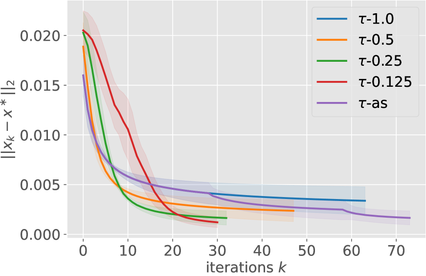
(a) Solutions distance.

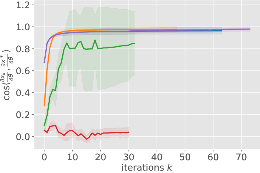
(b) Gradients similarity.

Figure 2: Gradients and solutions distance between CvxpyLayer and DFWLayer with different temperatures for medium-scale problems. All the curves terminate for tolerance $\epsilon=1e-4$. The shaded area for all the curves stands for standard deviation over 5 trials and $x^{\ast}$ stands for solutions obtained by CvxpyLayer.

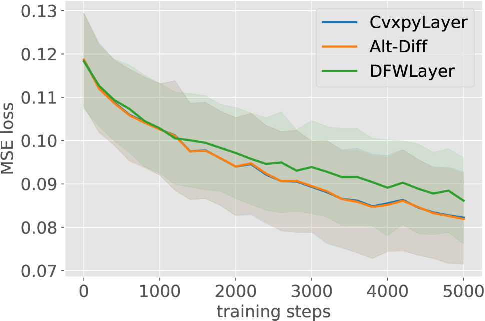
(a) MSE loss.

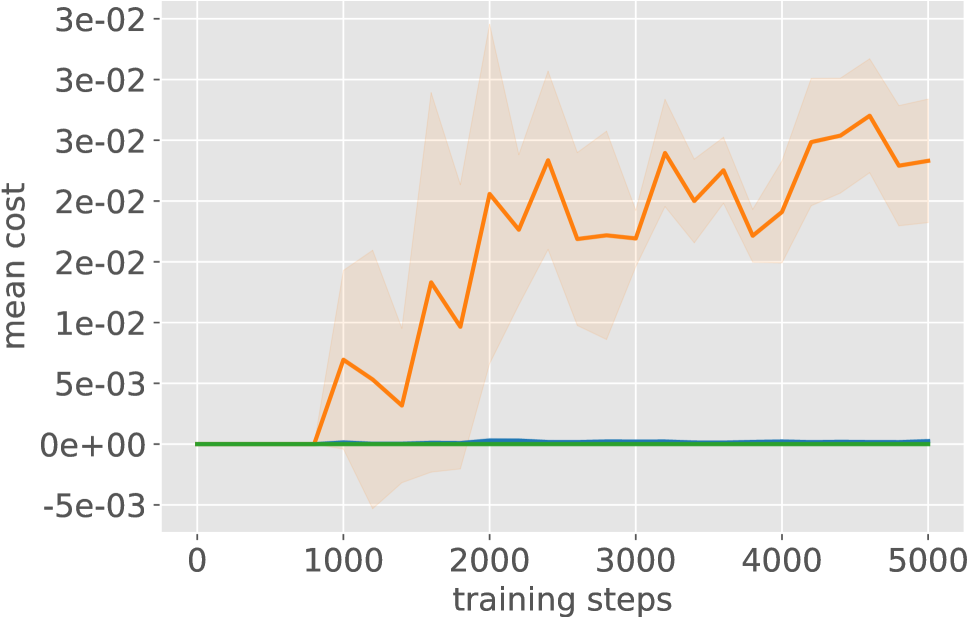
(b) Mean violation.

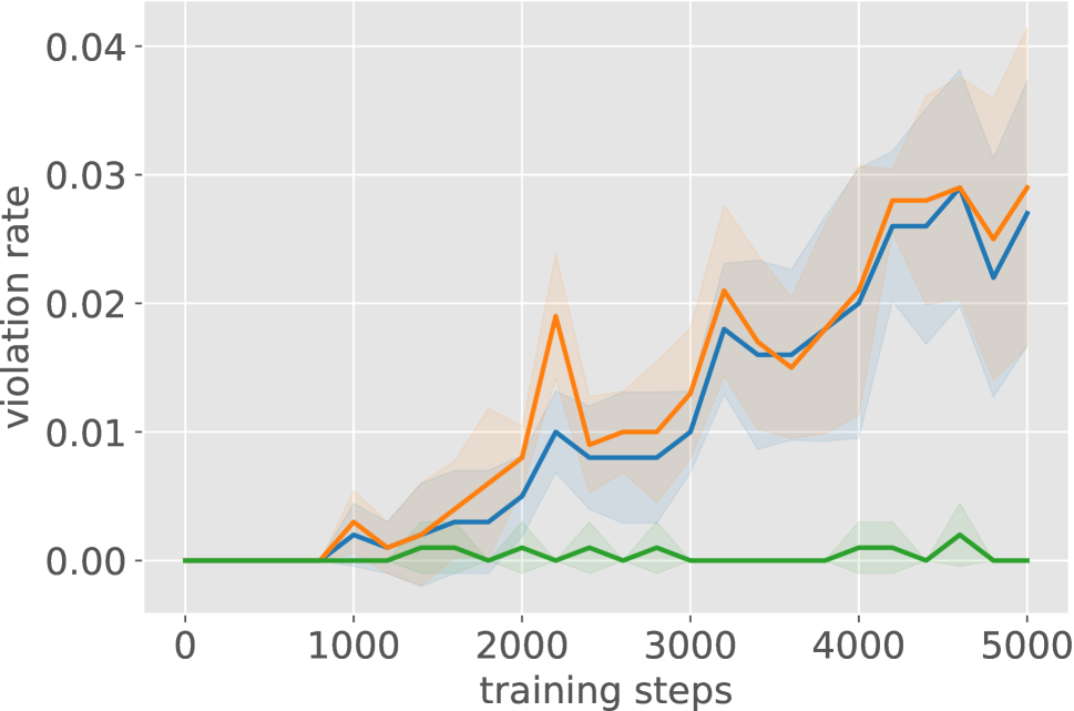
(c) Violation rate.

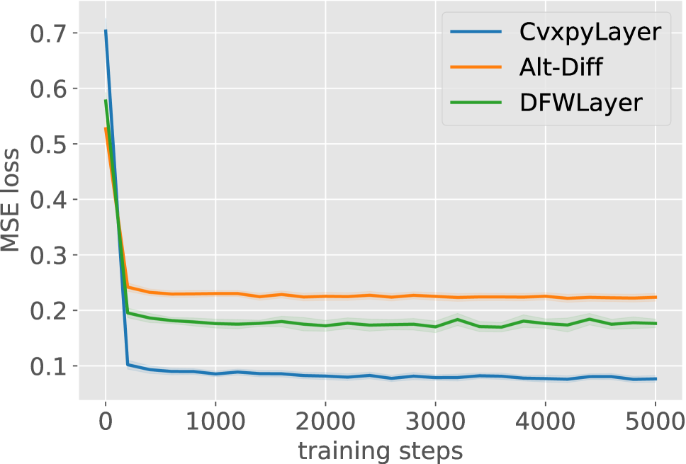
(d) MSE loss.

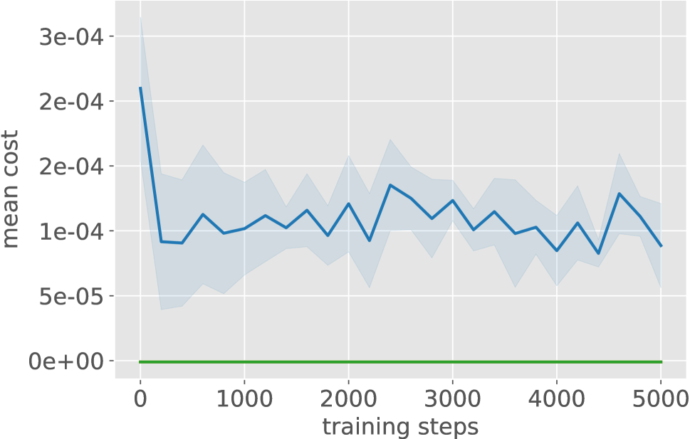
(e) Mean violation.

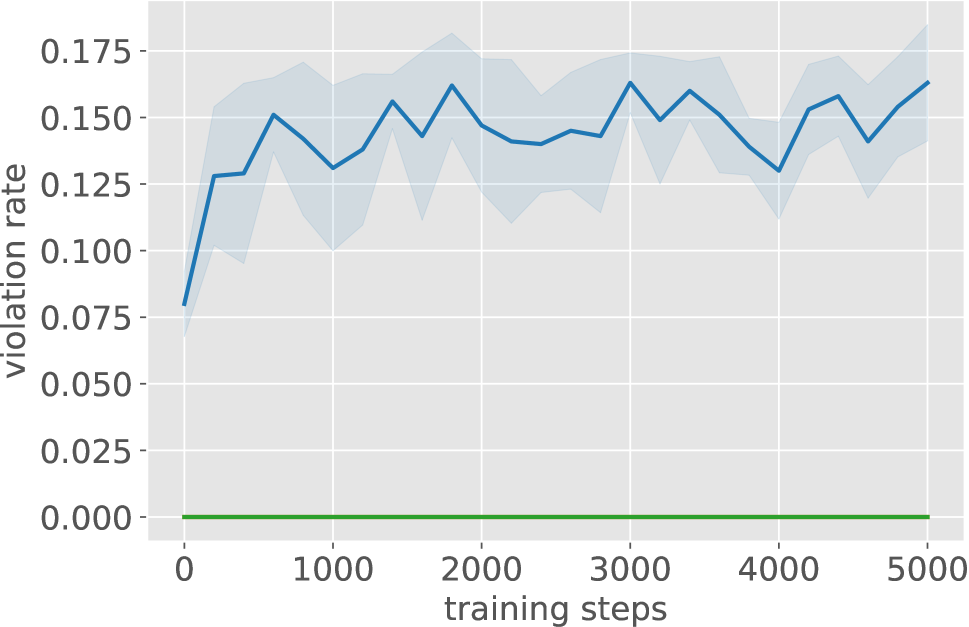
(f) Violation rate.

Figure 3: MSE loss, mean violation and violation rate for robotics tasks. The first row is for R+O03 and the second row is for HC+O. Mean violation is computed over violated samples and violation rate is the ratio of violated samples to all samples in the testing set. The shaded area for all the curves stands for standard deviation over 5 trials. Lower values are better for all the metrics.

It can be seen from Figure 2(a) that with the decrease of temperature the accuracy of solutions obtained by DFWLayer becomes higher, as shown in 5.3. However, the automatic differentiation involving a small temperature can be unstable after a large number of iterations. As presented in Figure 2(b), DFWLayer fails to compute accurate gradients when the temperature decreases to $\tau=0.25$ and $\tau=0.125$. Therefore, we choose to use an annealing temperature so that our method can obtain high-quality solutions and gradients at the same time, which is validated by the curve ”$\tau$-as” (the purple lines) in Figure 2.

Robotics Tasks Under Imitation Learning

As for the field of robotics, in this subsection, we discuss the application of our method to specific tasks under an imitation learning framework. HC+O and R+O03 are constrained HalfCheetah and Reacher environments chosen from action-constrained-RL-benchmark in Kasaura et al. (2023). The original enviroments are from OpenAI Gym (Brockman et al. 2016) and PyBullet-Gym (Ellenberger 2018–2019) and the constraints are presented as follows:

$$\sum_{i}^{d}\lvert w_{i}a_{i}\rvert\leq p_{\rm max},$$ (15)

where $w_{i}$ and $a_{i}$ are the angular velocity and the torques corresponding to $d$ joints, respectively, and $p_{\rm max}$ stands for the power constraint. Specifically, $d=6$ and $p_{\rm max}=20.0$ are for HC+O, while $d=2$ and $p_{\rm max}=0.3$ are for R+O03.

Under an imitation learning framework, optimization layers are added to the neural networks as the last layer, which aims to imitate expert policy and satisfy the power constraints (15). We first collected 1 million and 0.3 million expert demonstrations by running DPro, a variant of TD3 in Kasaura et al. (2023), for HC+O and R+O03 respectively. Then, imitation learning was implemented using 80% data as the training set with the MSE loss function. During the training phase, we tested the loss, mean violation and violation rate every 200 steps using the rest 20% data as the testing set. Other details are referred to Appendix B.

As is shown in Figure 3, DFWLayer has significantly lower mean violation and violation rate than the other two baselines with comparable MSE loss. For R+O03 whose maximum power $p_{\rm max}=0.3$, the magnitude of the mean violation (about 3e-2) for Alt-Diff would have negative influence on the robotics tasks. However, DFWLayer and CvxpyLayer (with minor violation) are able to give feasible solutions to accomplish the tasks with accuracy and safety. For HC+O whose maximum power $p_{\rm max}=20.0$, CvxpyLayer achieves the best MSE loss with minor violation and a relatively high violation rate, while Alt-Diff satisfies the constraints all the time with the worst MSE loss. By contrast, DFWLayer outperforms the two methods comprehesively.

7 Conclusions

In this paper, we have proposed DFWLayer for solving convex optimization problems with $L$-smooth functions and hard-to-project norm constraints in an efficient way. Naturally derived from the Frank-Wolfe, DFWLayer accelerates to obtain solutions and gradients based on first-order optimization methods which avoid projections and Hessian matrix computations. Especially for $\ell_{1}$-norm constraints, DFWLayer replaces non-differentiable operators with probabilistic approximation so that gradients can be efficiently computed through the unrolling sequence with automatic differentiation. Also, we have shown the convergence of DFWLayer by bounding the suboptimality gap with the decreasing MMD between the approximating and the target distributions. Thus, an annealing temperature is designed to guarantee the quality of both solutions and gradients. Comprehensive experiments have demonstrated the efficiency and accuracy of DFWLayer compared to the state-of-the-art methods. However, there are still some potential limitations to be highlighted. First, the convergence rate can be further enhanced to linear rate by other variants of the Frank-Wolfe, such as Away-Step Frank-Wolfe (Guélat and Marcotte 1986) and Pairwise Frank-Wolfe (Lacoste-Julien et al. 2013). Second, the running time for DFWLayer increases when dealing with multiple optimization problems. The parallel computation mechanism, which has been implemented by Optnet, should be added to DFWLayer.

Supplementary Material

The organization of supplementary is as follows:

• Appendix A: Proof of 5.3;

• Appendix B: Experimental details for Section 6.

Appendix A Proof

As stated in the proof sketch Section 5, we can first split it into two terms,

$$h(\hat{x}_{k}) =f(\hat{x}_{k})-f(x^{\ast})$$

$$=\underbrace{f(\hat{x}_{k})-f(x_{k})}_{\text{approximation gap}}+\underbrace{f(x_{k})-f(x^{\ast})}_{\text{origin gap}}.$$

The original gap of the Frank-Wolfe with the short path rule and its proof are provided by Braun et al. (2022), we restate it as the following lemma.

Lemma A.1.

Let $f:\mathbb{R}^{n}\rightarrow\mathbb{R}$ be a L-smooth convex function on a convex region $\mathcal{C}$ with diameter $M$. The Frank-Wolfe with short path rule converges as follows:

$$h(x_{k})=f(x_{k})-f(x^{\ast})\leq\frac{2LM^{2}}{k+3}\leq\frac{2LM^{2}}{k+2}.$$

Then, we need to present a useful remark, which is used for the proof of A.1 in (Braun et al. 2022) and the following proof of 5.3.

Remark A.2.

In essence, the proof of 5.3 uses the modified agnostic step size $\gamma_{k}=\frac{2}{k+3}$, instead of the standard agnostic step size $\gamma_{k}=\frac{2}{k+2}$, because the convergence rate for the short path rule dominates the modified agnostic step size.

With A.1 and A.2, we now start to prove 5.3.

Proof of 5.3.

The original solutions $x_{k}$ can be recursively expressed as the combination of initial $x_{0}$ and vertex $s_{k}$ at each iteration,

$$x_{k} =(1-\gamma)x_{k-1}+\gamma s_{k-1}$$

$$=(1-\gamma)((1-\gamma)x_{k-2}+\gamma s_{k-2})+\gamma s_{k-1}$$

$$=(1-\gamma)^{k}x_{0}+\gamma\sum_{o}^{k-1}(1-\gamma)^{k-1-i}s_{i}.$$ (16)

Similar with the original solutions, the solutions obtained by DFWLayer can also be derived as follows:

$$\hat{x}_{k}=(1-\gamma)^{k}x_{0}+\gamma\sum_{o}^{k-1}(1-\gamma)^{k-1-i}\hat{s}_{i}.$$ (17)

And thus we subtract (A) from (17) and obtain

$$\hat{x}_{k}-x_{k}=\gamma\sum_{o}^{k-1}(1-\gamma)^{k-1-i}(\hat{s}_{i}-s_{i}).$$ (18)

Considering the smoothness of $f$ and (18), the approximation can be derived as

$$f(\hat{x}_{k})-f(x_{k}) \leq\langle\nabla_{x}f(x_{k}),\hat{x}_{k}-x_{k}\rangle+\frac{L}{2}\lVert\hat{x}_{k}-x_{k}\rVert^{2}$$

$$=\gamma\sum_{0}^{k-1}(1-\gamma)^{k-1-i}\nabla_{x}f(x_{k})^{T}(\hat{s}_{i}-s_{i})$$

$$+\frac{L}{2}\lVert\gamma\sum_{0}^{k-1}(1-\gamma)^{k-1-i}(\hat{s}_{i}-s_{i})\rVert^{2}$$

$$\leq\gamma\sum_{0}^{k-1}(1-\gamma)^{k-1-i}(\mathbb{E}_{s\sim\hat{p}_{i}}[\nabla_{x}f(x_{k})^{T}s]$$

$$-\mathbb{E}_{s\sim p_{i}}[\nabla_{x}f(x_{k})^{T}s])$$

$$+\frac{L}{2}\gamma^{2}\sum_{0}^{k-1}(1-\gamma)^{2(k-1-i)}\lVert\hat{s}_{k}-s_{k}\rVert^{2}$$

$$\leq\gamma\sum_{0}^{k-1}(1-\gamma)^{k-1-i}\delta$$

$$+\frac{L}{2}\gamma^{2}\sum_{0}^{k-1}(1-\gamma)^{2(k-1-i)}M^{2}$$

$$=(1-(1-\gamma)^{k})\delta$$

$$+\frac{LM^{2}}{2}\frac{\gamma}{2-\gamma}(1-(1-\gamma)^{2k})$$

$$\leq\delta+\frac{LM^{2}}{2k+4}.$$

Here, we use the triangle inequality in the first inequality. Then, we bound the difference of expectations by $\delta$ under 5.1 and the distance between vertices by region diameter $M$ in the second inequality. The last equality is obtained by choosing $\gamma_{k}=\frac{2}{k+3}$ via heuristic in A.2.

Therefore, substituting the approximation gap from A.1 and the origin gap in (12) yields (11) as claimed. ∎

Appendix B Experimental Details

Augmented Optimization Problem

In order to directly leverage Alt-Diff, we augment the variables with additional variables $z\in\mathbb{R}^{n}$ such that $y=\Big{[}x^{T},z^{T}\Big{]}^{T}\in\mathbb{R}^{2n}$ and obtain an augmented optimization problem as follows:

$$\min_{y}f(y;\theta)\ \ \ \ \text{s.t.}\ Gy\leq h,,$$

Table 3: Comparison of accuracy w.r.t. solutions and gradients for small-scale problems. The average and standard deviation are obtained over 5 trials. Higher values are better for the gradients similarity, while lower values are better for other metrics. Constraints violation are shown in red. Gradients similarity and solutions distance are computed with those obtained by CvxpyLayer as the reference.

	Gradients Sim.	Solutions Dist.	Mean Violation	Max Violation
CvxpyLayer	1.000 $\pm$ 0.000	0.000 $\pm$ 0.000	0.000	0.000
Alt-Diff	0.975 $\pm$ 0.049	0.002 $\pm$ 0.003	0.063	1.000
DFWLayer	0.977 $\pm$ 0.025	0.002 $\pm$ 0.001	0.000	0.000

Table 4: Comparison of accuracy w.r.t. solutions and gradients for large-scale problems. The average and standard deviation are obtained over 5 trials. Higher values are better for the gradients similarity, while lower values are better for other metrics. Constraints violation are shown in red. Gradients similarity and solutions distance are computed with those obtained by CvxpyLayer as the reference.

	Gradients Sim.	Solutions Dist.	Mean Violation	Max Violation
CvxpyLayer	1.000 $\pm$ 0.000	0.000 $\pm$ 0.000	0.000	0.000
Alt-Diff	0.978 $\pm$ 0.044	0.001 $\pm$ 0.001	0.061	1.000
DFWLayer	0.978 $\pm$ 0.023	0.001 $\pm$ 0.001	0.000	0.000

Then, $\ell_{1}$-norm constraints $\lVert w\circ x\rVert_{1}\leq t$ into a set of constraints through absolute value decomposition,

$$-w_{i}x_{i}-z_{i}\leq 0,$$

$$w_{i}x_{i}-z_{i}\leq 0,$$

$$-z_{i}\leq 0,$$

$$\sum_{i}z_{i}\leq t,$$

where $i=1,...,n$. Thus, the parameters $G\in\mathbb{R}^{(3n+1)\times 2n}$ and $h\in\mathbb{R}^{3n+1}$ for matrix form constraints $Gy\leq h$ are as follows:

$$G=\left[\begin{array}[]{cccccc}-w_{1}&&&-1&&\\ &\ddots&&&\ddots&\\ &&-w_{n}&&&-1\\ w_{1}&&&-1&&\\ &\ddots&&&\ddots&\\ &&w_{n}&&&-1\\ 0&&&-1&&\\ &\ddots&&&\ddots&\\ &&0&&&-1\\ 0&\ldots&0&1&\ldots&1\end{array}\right],h=\left[\begin{array}[]{c}0\\ \vdots\\ 0\\ t\end{array}\right].$$

Similarly, the original objective should also be converted to an augmented one. As for quadratic objective used in Section 6, the augmented parameters $P_{\rm aug}$ and $q_{\rm aug}$ are as follows:

$$P_{\rm aug}=\left[\begin{array}[]{cccccc}&&&&&\\ &P&&&&\\ &&&&&\\ &&&0&&\\ &&&&\ddots&\\ &&&&&0\\ \end{array}\right],q_{\rm aug}=\left[\begin{array}[]{c}\\ q\\ \\ 0\\ \vdots\\ 0\\ \end{array}\right].$$

Therefore, the augmented optimization problem can be used by Alt-Diff in all the experiments.

Additional Experimental Results

Due to space limitation, we only present the comparison of accuracy w.r.t. solutions and gradients for medium problems in the first set of experiments. Here, we give the results for the other problem sizes.

We can see that DFWLayer still has competitive accuracy of solutions and gradients compared with Alt-Diff. In addition, DFWLayer and CvxpyLayer can always satisfy the constraints, while Alt-Diff violates the constraints in other problems sizes.

Hyperparameters for Robotics Tasks

The architecture for previous layers is $[400,300]$ and the activation function is ${\rm ReLU}$ function. The parameters are updated by Adams optimizer with $1e-4$ as the learning rate. As for batch size, we have some experiments from {8, 16, 32, 64, 128}, and choose to use 64 considering the performance and efficiency comprehensively.

References

- Abadi et al. (2016) Abadi, M.; Agarwal, A.; Barham, P.; Brevdo, E.; Chen, Z.; Citro, C.; Corrado, G. S.; Davis, A.; Dean, J.; Devin, M.; et al. 2016. Tensorflow: Large-scale machine learning on heterogeneous distributed systems. arXiv preprint arXiv:1603.04467.
- Agrawal et al. (2019) Agrawal, A.; Amos, B.; Barratt, S.; Boyd, S.; Diamond, S.; and Kolter, J. Z. 2019. Differentiable convex optimization layers. Advances in neural information processing systems, 32.
- Amos (2019) Amos, B. 2019. Differentiable Optimization-Based Modeling for Machine Learning. Ph.D. thesis, Carnegie Mellon University.
- Amos and Kolter (2017) Amos, B.; and Kolter, J. Z. 2017. Optnet: Differentiable optimization as a layer in neural networks. In International Conference on Machine Learning, 136–145. PMLR.
- Bambade et al. (2023) Bambade, A.; Schramm, F.; Taylor, A.; and Carpentier, J. 2023. QPLayer: efficient differentiation of convex quadratic optimization. Optimization.
- Braun et al. (2022) Braun, G.; Carderera, A.; Combettes, C. W.; Hassani, H.; Karbasi, A.; Mokhtari, A.; and Pokutta, S. 2022. Conditional gradient methods. arXiv preprint arXiv:2211.14103.
- Brockman et al. (2016) Brockman, G.; Cheung, V.; Pettersson, L.; Schneider, J.; Schulman, J.; Tang, J.; and Zaremba, W. 2016. OpenAI Gym. arXiv:1606.01540.
- Chen et al. (2021) Chen, B.; Donti, P. L.; Baker, K.; Kolter, J. Z.; and Bergés, M. 2021. Enforcing Policy Feasibility Constraints through Differentiable Projection for Energy Optimization. In Proceedings of the Twelfth ACM International Conference on Future Energy Systems, e-Energy ’21, 199–210. New York, NY, USA: Association for Computing Machinery. ISBN 9781450383332.
- Dalle et al. (2022) Dalle, G.; Baty, L.; Bouvier, L.; and Parmentier, A. 2022. Learning with combinatorial optimization layers: a probabilistic approach. arXiv preprint arXiv:2207.13513.
- Domahidi, Chu, and Boyd (2013) Domahidi, A.; Chu, E.; and Boyd, S. 2013. ECOS: An SOCP solver for embedded systems. In European Control Conference (ECC), 3071–3076.
- Donti, Rolnick, and Kolter (2020) Donti, P. L.; Rolnick, D.; and Kolter, J. Z. 2020. DC3: A learning method for optimization with hard constraints. In International Conference on Learning Representations.
- Ellenberger (2018–2019) Ellenberger, B. 2018–2019. PyBullet Gymperium. https://github.com/benelot/pybullet-gym.
- Frank, Wolfe et al. (1956) Frank, M.; Wolfe, P.; et al. 1956. An algorithm for quadratic programming. Naval research logistics quarterly, 3(1-2): 95–110.
- Ghadimi and Wang (2018) Ghadimi, S.; and Wang, M. 2018. Approximation methods for bilevel programming. arXiv preprint arXiv:1802.02246.
- Guélat and Marcotte (1986) Guélat, J.; and Marcotte, P. 1986. Some comments on Wolfe’s ‘away step’. Mathematical Programming, 35(1): 110–119.
- Jaggi (2013) Jaggi, M. 2013. Revisiting Frank-Wolfe: Projection-free sparse convex optimization. In International conference on machine learning, 427–435. PMLR.
- Kasaura et al. (2023) Kasaura, K.; Miura, S.; Kozuno, T.; Yonetani, R.; Hoshino, K.; and Hosoe, Y. 2023. Benchmarking Actor-Critic Deep Reinforcement Learning Algorithms for Robotics Control with Action Constraints. IEEE Robotics and Automation Letters.
- Lacoste-Julien et al. (2013) Lacoste-Julien, S.; Jaggi, M.; Schmidt, M.; and Pletscher, P. 2013. Block-coordinate Frank-Wolfe optimization for structural SVMs. In International Conference on Machine Learning, 53–61. PMLR.
- Landry (2021) Landry, B. 2021. Differentiable and Bilevel Optimization for Control in Robotics. Stanford University.
- Lin et al. (2021) Lin, J.-L.; Hung, W.; Yang, S.-H.; Hsieh, P.-C.; and Liu, X. 2021. Escaping from zero gradient: Revisiting action-constrained reinforcement learning via Frank-Wolfe policy optimization. In Uncertainty in Artificial Intelligence, 397–407. PMLR.
- O’Donoghue (2021) O’Donoghue, B. 2021. Operator Splitting for a Homogeneous Embedding of the Linear Complementarity Problem. SIAM Journal on Optimization, 31: 1999–2023.
- Paszke et al. (2019) Paszke, A.; Gross, S.; Massa, F.; Lerer, A.; Bradbury, J.; Chanan, G.; Killeen, T.; Lin, Z.; Gimelshein, N.; Antiga, L.; et al. 2019. Pytorch: An imperative style, high-performance deep learning library. Advances in neural information processing systems, 32.
- Sanket et al. (2020) Sanket, S.; Sinha, A.; Varakantham, P.; Andrew, P.; and Tambe, M. 2020. Solving online threat screening games using constrained action space reinforcement learning. In Proceedings of the AAAI Conference on Artificial Intelligence, volume 34, 2226–2235.
- Stechlinski, Khan, and Barton (2018) Stechlinski, P.; Khan, K. A.; and Barton, P. I. 2018. Generalized sensitivity analysis of nonlinear programs. SIAM Journal on Optimization, 28(1): 272–301.
- Sun et al. (2022) Sun, H.; Shi, Y.; Wang, J.; Tuan, H. D.; Poor, H. V.; and Tao, D. 2022. Alternating Differentiation for Optimization Layers. In The Eleventh International Conference on Learning Representations.
- Yeh et al. (2022) Yeh, R. A.; Hu, Y.-T.; Ren, Z.; and Schwing, A. G. 2022. Total Variation Optimization Layers for Computer Vision. In Proceedings of the IEEE/CVF Conference on Computer Vision and Pattern Recognition, 711–721.