Cost-Efficient Online Decision Making: A Combinatorial Multi-Armed Bandit Approach

Abstract

Online decision making plays a crucial role in numerous real-world applications. In many scenarios, the decision is made based on performing a sequence of tests on the incoming data points. However, performing all tests can be expensive and is not always possible. In this paper, we provide a novel formulation of the online decision making problem based on combinatorial multi-armed bandits and take the (possibly stochastic) cost of performing tests into account. Based on this formulation, we provide a new framework for cost-efficient online decision making which can utilize posterior sampling or BayesUCB for exploration. We provide a theoretical analysis of Thompson Sampling for cost-efficient online decision making, and present various experimental results that demonstrate the applicability of our framework to real-world problems.

1 Introduction

Online decision making (ODM) is concerned with interactions of an agent with an environment through a series of sequential tests in order to acquire sufficient information about the environment and successively learn how to make better decisions. Each such test and decision can be associated with either a reward or a cost. Here, we focus on problem settings where tests may incur stochastic costs.

One such example is medical diagnosis. A patient arrives at a hospital with an unknown affliction. In order to determine an appropriate treatment for the patient, a number of medical tests need to be performed. Since each of these tests might take time (which can differ depending on the test result and the underlying affliction), be expensive or cause discomfort to the patient, it is desirable to limit the set of tests to the most informative ones. On the other hand, it is apparent that misdiagnosing the patient can have severe consequences, so performing too few tests is also undesirable.

Another example is adaptive identification of driver preferences for in-car navigation systems. Consider the selection of charging stations during long-distance trips with battery-electric vehicles (BEVs). Since the duration of a single charging stop can be as long as 40 minutes, it may be desirable to select a charging station with additional amenities in close proximity, such as restaurants, shops, or public restrooms. While it is possible to ask questions through the vehicle user interface of drivers to learn their charging location preferences, such questions should be kept few, short, and simple. We note that in both of these examples, the problem instances (e.g., diagnosis of patients and identification of driver preferences) arrive incrementally in an online manner and should be processed accordingly.

We take a novel view of the online decision making problem described above, where we cast it as a combinatorial multi-armed bandit problem (CMAB) (Cesa-Bianchi and Lugosi, 2012), an extension of the classical multi-armed bandit problem (MAB). The standard MAB problem is a common way of representing the trade-off inherent to decision making problems between exploring an environment by performing successive actions (playing arms, in bandit nomenclature) to gain more knowledge and exploiting that knowledge to reach a long-term objective. In a CMAB problem, an agent interacts with the environment in each time step by performing a set of actions (a super arm), where the set may be subject to combinatorial constraints. Each individual action (base arm) in that set may result in some observed feedback (so-called semi-bandit feedback), and the agent also receives a reward associated with the complete super arm.

In this work, we view the combined choice of tests to perform and the selected decision as a super arm in a CMAB problem where the underlying cost distribution parameters are initially unknown, which allows us to leverage effective MAB exploration strategies like Thompson Sampling (TS) (Thompson, 1933) and Upper Confidence Bound (UCB) (Auer et al., 2002) together with cost-efficient (active) information acquisition methods, such as Equivalent Class Edge Cutting (EC²) (Golovin et al., 2010) and Information Gain (IG) (Dasgupta, 2005). We summarize our contributions as follows.

1. We study the problem of cost-efficient online decision making, where costs may be stochastic and depend on both test and decision outcomes. For this, we propose a novel combinatorial semi-bandit framework, providing a new perspective on cost-efficient information acquisition.

2. We adapt a number of bandit methods to this framework, namely Thompson Sampling and Upper Confidence Bound, combined with novel extensions of EC² and IG which can handle tests with different and stochastic costs, which we call W-EC² and W-IG, respectively. Thereby, in addition to Thompson Sampling, we develop W-EC² and W-IG oracles utilizing a Bayesian variant of UCB (called BayesUCB by Kaufmann et al. 2012) that is well adapted to our framework and enables the UCB method to effectively employ prior knowledge in the form of a prior distribution.

3. We demonstrate the effectiveness of our framework via several experimental studies performed on data sets from a variety of important domains. We find that Thompson Sampling yields the best performance in most of the experiments we perform.

4. We theoretically analyze the performance of Thompson Sampling within our framework for cost-efficient online decision making and establish an upper bound on its Bayesian regret.

2 Related Work

Cost-efficient information acquisition.

The primary goal of cost-efficient information acquisition algorithms is to sequentially select from a number of available costly tests to make a decision (such as making a prediction about a label) with a minimal cost. To minimize cost, these tests are performed until a sufficient level of confidence in the decision is reached. Prominent algorithms for cost-efficient information acquisition are Information Gain (IG) (Zheng et al., 2012), EC² (Golovin et al., 2010), and Uncertainty Sampling (US). Among them, EC² has been proved to enjoy adaptive submodularity (Golovin et al., 2010), and thus yields near-optimal cost. The works of Rahbar et al. (2023); Chen et al. (2017) consider active information acquisition in an online setting. The regret bounds in these works are based on formulating the problem as a Partially Observable Markov Decision Process (POMDP) and are exponential in the total number of possible tests. In this work, we consider a CMAB formulation of the problem and derive a regret bound that is linear in the number of tests (and sublinear w.r.t. the horizon $T$). In addition, unlike Rahbar et al. (2023); Chen et al. (2017), our framework supports variability in the cost of the tests depending on the outcomes of the tests and the decisions.

Combinatorial semi-bandit algorithms.

CMAB methods have been utilized to address online learning problems in various settings but often without considering cost-efficient information acquisition. Durand and Gagné (2014) adapt a combinatorial variant of Thompson Sampling for online feature selection where the agent has a fixed budget for tests and the reward is a linear function of the test outcomes. Both assumptions are used in later works studying the problem from a CMAB perspective (Bouneffouf et al., 2017, 2021), but differ from the setting considered in this work (e.g., the budget for information acquisition is fixed with no concept of achieving a decision, and the costs are independent of the outcomes of the tests and the decisions). Åkerblom et al. (2023) analyze the Bayesian regret of combinatorial Thompson Sampling using a similar technique as this work (originally developed by Russo and Van Roy (2014) for standard and linear MAB), but for a very different super arm reward function and setting (for the online minimax path problem, which does not consider cost-efficient information acquisition and decision making).

3 Problem Formulation

In this section, we propose a new formulation of the online decision making problem which incorporates the cost of acquiring test outcomes. In each time step $t$, we receive the problem instance (e.g., data point) $\mathbf{x}^{(t)}$ with $n$ tests $\{x_{1}^{(t)},x_{2}^{(t)},\dots,x_{n}^{(t)}\}$. Here, we assume that all test outcomes (unknown until after each test is performed) are binary (i.e., $x_{i}^{(t)}\in\{0,1\}$ for all $i$), but our methods can easily be extended to other test values (see Section 6). The goal is to make an accurate decision $y^{(t)}\in[m]$ for that problem instance with a minimal cost of performing tests ($m$ represents the total number of options for the decision, or outcomes if the correct decision is viewed as a random variable), where we denote the correct decision by $y^{*}$.

Consistent with the common Naïve Bayes assumption, we let all tests $x_{i}^{(t)}$ be mutually independent and Bernoulli-distributed conditional on the decision $y^{(t)}$. We also let $y^{*}$ be known given a full realization of $\mathbf{x}^{(t)}$. This implies that upon performing all available tests, we know the correct decision for the problem instance. This is realistic and consistent with the settings of Golovin et al. (2010); Chen et al. (2017); Rahbar et al. (2023), though they do not follow a CMAB formulation. As an example, consider a medical diagnosis problem. This property means that if we perform all available medical tests, we can determine the correct diagnosis.

Regarding the costs, we assume that they directly depend on the outcomes of the tests and the decisions. As motivation, consider, for example, a medical test to confirm the presence of some indicator for a particular disease. If such an indicator is found, the test can be terminated immediately with a positive outcome, whereas establishing the non-presence of an indicator (for a negative test outcome) may require more time and be more invasive.

We model the problem described above by an elegant design of a stochastic combinatorial multi-armed bandit (CMAB) problem (Cesa-Bianchi and Lugosi, 2012) with semi-bandit feedback. Briefly, CMAB corresponds to a reward maximization problem with a set of base arms. In each time step, the agent selects a subset of base arms. After playing this subset of base arms, called a super arm, the agent receives a reward from the environment. The objective is to maximize the expected sum of rewards within a time horizon $T$, which is typically formulated as a regret minimization task.

In our problem, since the costs of tests depend on both test and decision outcomes, we need to consider a set of base arms that reflect both. Therefore, we define the set $\mathcal{A}$ of $n\times m$ base arms $a_{ij}$ ($i\in[n]$ and $j\in[m]$). In each time step $t$, the agent selects a super arm $S^{(t)}\in 2^{\mathcal{A}}$ and receives the reward $R(S^{(t)})=R^{(t)}$. A base arm $a_{ij}$ in $S^{(t)}$ indicates that the test with index $i$ is performed for making decision $y^{(t)}=j$. We define $\mathcal{I}^{(t)}\subseteq 2^{\mathcal{A}}$ as the set of feasible super arms at time $t$ which yield a decision, i.e., each feasible super arm consists of tests and a single decision (concretely, if $a_{ij},a_{lk}\in S\in\mathcal{I}^{(t)}$, then $j=k$). The feedback at time $t$ of a base arm $a_{ij}\in\mathcal{A}$ (observable by the agent if $a_{ij}\in S^{(t)}$) is the corresponding outcome of test $x_{i}^{(t)}$, which given a decision $y^{(t)}=j$ is Bernoulli-distributed with an unknown (to the agent) parameter $\theta_{ij}\triangleq Pr(x_{i}=1|y=j)$, for all $i,j$. While tests may, in practice, be selected sequentially, the super arm (and base arms) are only known in hindsight after the decision has been made. This is intentional and allows us to analyze the problem as a CMAB.

We let the cost (assumed to be fixed and known) of each base arm $a_{ij}$ be $\mu_{ij}^{(0)}\in[0,1]$ and $\mu_{ij}^{(1)}\in[0,1]$ (given test outcomes $0$ and $1$, respectively). Then, we define the expected reward of the selected feasible super arm $S^{(t)}$ as the negative sum of expected base arm costs, such that $\mathbb{E}[R(S^{(t)})]=-\sum_{ij\in S}\mu_{ij}$, where

$$\mu_{ij}\triangleq\mu_{ij}^{(1)}\times\theta_{ij}+\mu_{ij}^{(0)}\times(1-\theta_{ij}),$$ (1)

with the vector of all $\mu_{ij}$’s denoted by $\boldsymbol{\mu}$ and the vector of all $\theta_{ij}$’s denoted by $\boldsymbol{\theta}$. We let $\boldsymbol{\mu}^{*}$ be the true underlying mean cost vector, with corresponding parameter vector $\boldsymbol{\theta}^{*}$. We define the suboptimality gap at time $t$ of a feasible super arm $S$ as

$$\Delta^{(t)}_{\boldsymbol{\mu}^{*}}(S)\triangleq f_{\boldsymbol{\mu}^{*}}(S^{*,(t)})-f_{\boldsymbol{\mu}^{*}}(S),$$ (2)

where $f_{\boldsymbol{\gamma}}(M)\triangleq(-\sum_{ij\in M}\gamma_{ij})$ denotes the expected reward of super arm $M$ given an arbitrary mean cost vector $\boldsymbol{\gamma}$, and $S^{*,(t)}\triangleq\operatorname*{argmax}_{S\in\mathcal{I}^{(t)}}f_{\boldsymbol{\mu}^{*}}(S)$ is the optimal super arm found by the oracle applied on the feasible set $\mathcal{I}^{(t)}$. Then, the regret (which the agent should minimize) for a time horizon $T$ is defined as

$$\text{Regret}_{\boldsymbol{\mu}^{*}}(T)\triangleq\sum_{t\in[T]}\Delta^{(t)}_{\boldsymbol{\mu}^{*}}(S^{(t)}).$$ (3)

4 CMAB Methods for ODM

In our framework, we utilize oracles (i.e., optimization algorithms) which, given a parameter vector $\boldsymbol{\theta}$, output super arms with maximum expected reward (or approximately, in the case of approximate oracles), such that

$$Oracle(\boldsymbol{\theta})\triangleq\operatorname*{argmax}_{S\in\mathcal{I}^{(t)}}\mathbb{E}\left[R(S)\right|\boldsymbol{\theta}].$$ (4)

The $\theta_{ij}^{*}$ values of the true parameter vector $\boldsymbol{\theta}^{*}$ are initially unknown, but to be able to employ prior knowledge, we consider a prior distribution over $\theta_{ij}^{*}$’s. Formally, we assume that each $\theta_{ij}^{*}$ follows a Beta distribution, $\mathrm{Beta}(\alpha_{ij}^{(0)},\beta_{ij}^{(0)})$. We also assume a fixed and known distribution over decision outcomes, denoted by $P(y)$ (i.e., the learning agent knows the marginal distribution a priori). However, even if the oracle is assumed to always be able to find the correct decision (i.e., it only needs to minimize the number of tests), the optimization problem is NP-hard, and thus in practice, we use approximate oracles (introduced in Section 4.1).

A greedy method to address the problem defined in Section 3 is that in each time step $t$, we use an oracle with the current (MAP) estimate of $\boldsymbol{\theta}^{*}$. However, this greedy method may converge to a sub-optimal super arm due to lack of exploration. To balance exploration and exploitation, we adapt Thompson Sampling and BayesUCB to our problem.

Thompson Sampling.

Algorithm 1 summarizes our framework, with Thompson Sampling used as exploration method. In each time step $t$, we sample the parameters from the current posterior distribution (line 2). We then (in lines 3-4) use the oracle to get a super arm based on the sampled parameters, and perform the tests sequentially. Finally, we use Algorithm 2 to update the posterior distribution of the parameters. Algorithm 2 uses the fact that Beta distribution is conjugate prior to the Bernoulli distribution.

BayesUCB.

To utilize BayesUCB for exploration instead of Thompson Sampling, we have to modify lines 2-3 of Algorithm 1 such that instead of sampling parameters from the posterior distribution, we retrieve optimistic parameter estimates. Like Kaufmann et al. (2012) (done for classical bandits), we achieve this by utilizing quantiles of the posterior distribution. However, since neither gain function (Eq. 7 or Eq. 11) of the approximate oracles introduced in this section is monotonically increasing w.r.t. the provided parameter vector $\boldsymbol{\theta}$, a high value of a base arm parameter $\theta_{ij}$ does not necessarily mean that test $i$ is more likely to be selected. Hence, with $Q_{\lambda}(\eta)$ denoting the quantile function (such that under the distribution $\lambda$, $\text{Pr}\left(X\leq Q_{\lambda}(\eta)\right)=\eta$), we compute both an upper confidence bound $\overline{\theta}^{(t)}_{ij}=Q_{\text{Beta}(\alpha_{ij}^{(t)},\beta_{ij}^{(t)})}(1-1/t)$ and a lower confidence bound $\underline{\theta}^{(t)}_{ij}=Q_{\text{Beta}(\alpha_{ij}^{(t)},\beta_{ij}^{(t)})}(1/t)$ for each base arm $a_{ij}$, which we pass to the oracles. Then, while computing Eq. 7 and Eq. 11, whenever a high value for a term involving $\theta_{ij}$ makes the algorithm more likely to select test $i$, we use $\overline{\theta}^{(t)}_{ij}$ as an optimistic estimate, and correspondingly, $\underline{\theta}^{(t)}_{ij}$ for terms making $i$ less likely to be selected.

Algorithm 1 Cost-efficient online decision making

0:  $P(y)$; $\boldsymbol{\mu}$; prior parameters $(\alpha_{ij}^{(0)},\beta_{ij}^{(0)}$)’s

1:  for t = 1, 2, …, T do

2:     Sample $\theta_{ij}^{(t)}$ from $\mathrm{Beta}(\alpha_{ij}^{(t-1)},\beta_{ij}^{(t-1)})$ for all $i,j$.

3:     $S^{(t)}\leftarrow Oracle(\boldsymbol{\theta}^{(t)})$ (e.g., Algorithm 3).

4:     Make decision based on $S^{(t)}$, and observe $x_{i}^{(t)}$ for all $i$ such that $a_{ij}\in S^{(t)}$.

5:     Observe correct decision $y^{(t)}$.

6:     Call Algorithm 2 and obtain $\mathrm{Beta}(\alpha_{ij}^{(t)},\beta_{ij}^{(t)})$ for all $i,j$.

7:  end for

Algorithm 2 Posterior update

0:  $S^{(t)}$; $x_{i}^{(t)}$ for all $i$ such that $a_{ij}\in S^{(t)}$; $y^{(t)}=k$; $\alpha_{ij}^{(t-1)}$’s and $\beta_{ij}^{(t-1)}$’s

1:  for each $x_{i}^{(t)}$ do

2:     if $x_{i}^{(t)}=1$ then

3:        $\alpha_{ik}^{(t)}$ $\leftarrow$ $\alpha_{ik}^{(t-1)}+1$

4:     else

5:        $\beta_{ik}^{(t)}$ $\leftarrow$ $\beta_{ik}^{(t-1)}+1$

6:     end if

7:  end for

4.1 Cost-Efficient Approximate Oracles

Solving the optimization problem in Eq. 4 is intractable in general (see, e.g., Golovin et al. 2010; Chakaravarthy et al. 2007). Therefore, to implement line 3 of Algorithm 1, we propose two different approximate oracles using algorithms that greedily select tests to optimize a surrogate objective function, Information Gain (IG) (Zheng et al., 2012) and EC² (Golovin et al., 2010). We introduce extensions of IG and EC² to handle tests with stochastic costs, which we call Weighted IG (W-IG) and Weighted EC² (W-EC²) respectively. In both of these, all probabilities involved are computed using the fixed and known decision distribution $P(y)$ and the conditional distribution over test outcomes $P(\mathbf{x}|y)$ (determined by a given parameter vector $\boldsymbol{\theta}$, see line 3 in Algorithm 1). In particular, the dependence on $\boldsymbol{\theta}$ is omitted in the following section to simplify notation.

Before introducing W-IG and W-EC², we need to define the notions of hypothesis and decision region. We call a full realization of test outcomes (i.e., of all possible tests) a hypothesis. Therefore, with $n$ binary tests, we have $2^{n}$ different possible hypotheses. Let $\mathcal{H}\triangleq\{0,1\}^{n}$ be the set of all possible hypotheses for $n$ tests. We can partition $\mathcal{H}$ into $m$ disjoint sets. We call each of these disjoint sets a decision region. Each decision region corresponds to a decision $y\in[m]$. So our objective will be finding the correct decision region, for which the cost of performing tests is low. We want to emphasize that one important difference between these oracles and standard CMAB oracles is that they are interactive. In other words, during a single time step, they sequentially perform tests and observe outcomes to select subsequent tests and make a decision.

Weighted IG algorithm (W-IG).

In the standard IG algorithm, based on a set of previously observed test outcomes, we select the test that maximizes the reduction of entropy in the decision regions. Formally, the gain of a test $i$ in the IG algorithm is defined as:

$$\Delta_{\text{IG}}\left(i\mid\mathbf{x}_{\mathcal{P}}\right)\triangleq\mathbb{H}(y|\mathbf{x}_{\mathcal{P}})-\mathbb{E}_{x_{i}|\mathbf{x}_{\mathcal{P}}}[\mathbb{H}(y|\mathbf{x}_{\mathcal{P}\cup\{i\}})],$$ (5)

where $\mathcal{P}$ is the set of previously performed tests, and $\mathbf{x}_{\mathcal{P}}$ is the vector of results of tests in $\mathcal{P}$. The random variable for decision regions is denoted $y$, and $\mathbb{H}(z)$ is the Shannon entropy of a random variable $z$. In the W-IG algorithm, we sequentially perform tests that maximize $\Delta_{\text{IG}}\left(i\mid\mathbf{x}_{\mathcal{P}}\right)$ divided with the expected cost of test $i$ given the previously performed tests. In other words, after performing and observing the outcomes of the tests in $\mathcal{P}$, the next test to perform will be

$$i^{*}=\operatorname*{argmax}_{i\in([n]\setminus\mathcal{P})}\Delta_{\text{W-IG}}\left(i\mid\mathbf{x}_{\mathcal{P}}\right),$$ (6)

where

$$\Delta_{\text{W-IG}}\left(i\mid\mathbf{x}_{\mathcal{P}}\right)\triangleq\frac{\Delta_{\text{IG}}\left(i\mid\mathbf{x}_{\mathcal{P}}\right)}{\text{Cost($i$)}},$$ (7)

and

$$\text{Cost($i$)}\triangleq\sum_{j\in[m]}\sum_{q\in\{0,1\}}\mu_{ij}^{(q)}\times Pr\left(x_{i}=q,y=j\mid\mathbf{x}_{\mathcal{P}}\right),$$ (8)

given test outcome costs $\mu_{ij}^{(0)}$ and $\mu_{ij}^{(1)}$ for all $i,j$. We call the set of hypotheses $\mathcal{H}_{i}=\{h|P(x_{i}|h)>0\}$ consistent with the outcome of test $i$. We continue performing tests until all hypotheses in $\bigcap\limits_{i\in\mathcal{P}}\mathcal{H}_{i}$ belong to the same decision region, i.e., there is only one decision region remaining.

Weighted EC² algorithm (W-EC²).

The standard EC² algorithm starts with a graph with $\mathcal{H}$ as the set of nodes. We have an edge $(h,h^{\prime})$ between two hypotheses $h$ and $h^{\prime}$ if and only if they do not belong to the same decision region. The weight of an edge $(h,h^{\prime})$ is set to $w_{hh^{\prime}}=P(h\mid\mathbf{x}_{\mathcal{P}})\times P(h^{\prime}\mid\mathbf{x}_{\mathcal{P}})$ where $P(\cdot\mid\mathbf{x}_{\mathcal{P}})$ is the posterior distribution of a hypotheses after performing tests. Naturally, the weight of a set of edges $\mathcal{E}$ is defined as the sum of weights of edges in $\mathcal{E}$, i.e., $w(\mathcal{E})\triangleq\sum_{(h,h^{\prime})\in\mathcal{E}}w_{hh^{\prime}}$. We say that performing a test $i$ cuts an edge $(h,h^{\prime})$ if $h\notin\mathcal{H}_{i}$ or $h^{\prime}\notin\mathcal{H}_{i}$. We denote the set of edges cut by test $i$ with $K(i)$.

We now define the objective function for the EC² algorithm as

$$f_{\text{EC}^{2}}\left(\mathcal{P}\right)\triangleq w\left(\bigcup_{i\in\mathcal{P}}K(i)\right).$$ (9)

Based on the objective function above, we define the EC² gain of a test $i$ as

$$\Delta_{\text{EC}^{2}}\left(i\mid\mathbf{x}_{\mathcal{P}}\right)\triangleq\mathbb{E}_{x_{i}|\mathbf{x}_{\mathcal{P}}}\left[f_{\text{EC}^{2}}\left(\mathcal{P}\cup\{i\}\right)-f_{\text{EC}^{2}}\left(\mathcal{P}\right)\right],$$ (10)

and, similar to W-IG, the W-EC² gain as

$$\Delta_{\text{W-EC}^{2}}\left(i\mid\mathbf{x}_{\mathcal{P}}\right)\triangleq\frac{\Delta_{\text{EC}^{2}}\left(i\mid\mathbf{x}_{\mathcal{P}}\right)}{\text{Cost($i$)}},$$ (11)

with $\text{Cost}(i)$ defined as in Eq. 8.

Also like with W-IG, in the W-EC² algorithm, we sequentially perform tests that maximize $\Delta_{\text{W-EC}^{2}}\left(i\mid\mathbf{x}_{\mathcal{P}}\right)$. We stop performing tests when all edges are cut, meaning that there is only one decision region left.

To be able to implement W-IG and W-EC² (calculate $\Delta_{\text{W-IG}}$ and $\Delta_{\text{W-EC}\textsuperscript{2}}$), similar to standard IG and EC², we assume that the outcomes of the tests are conditionally independent given the decision. We show the test selection process in W-IG and W-EC² algorithms in Algorithm 3.

Algorithm 3 Cost-efficient approximate oracle

0:  $\text{Alg}\in\{\text{W-IG},\text{W-EC}^{2}\}$; $P(y)$; $\boldsymbol{\mu}$; $\boldsymbol{\theta}$

1:  Enumerate hypotheses in $\mathcal{H}$

2:  $\mathcal{P}=\{\}$

3:  while more than one decision region left do

4:     Select next test (with $\Delta_{\text{Alg}}(\cdot)$ computed w.r.t. $\boldsymbol{\theta}$) $i^{*}=\operatorname*{argmax}\limits_{i\in([n]\setminus\mathcal{P})}\Delta_{\text{Alg}}\left(i\mid\mathbf{x}_{\mathcal{P}}\right)$.

5:     Perform test $i^{*}$ and observe $x_{i^{*}}$.

6:     Update $P(h\mid\mathbf{x}_{\mathcal{P}})$ based on results of tests in $\mathcal{P}$.

7:  end while

8:  Select the decision associated to the remaining decision region.

5 Theoretical Analysis

In this section, we theoretically analyze the framework proposed in Section 4. Specifically, we provide an upper bound on the Bayesian regret (defined below) of the online decision making procedure in Algorithm 1.

In our problem setting, the set of feasible super arms $\mathcal{I}^{(t)}$ is restricted such that $y^{(t)}=y^{*}$ (i.e., we study the setting where correct decisions are guaranteed, and the objective is to minimize the cost of tests), and we assume that we have access to a perfect oracle which can solve the optimization problem Eq. 4.

The Bayesian regret is defined as the expected value of $\text{Regret}(T)$ (see Eq. 3), with the expectation taken over the prior distribution of $\boldsymbol{\mu}^{*}$ and other random variables (e.g., randomness in the rewards and the policy of the agent).

$$\text{Bayesian Regret}(T)\triangleq\mathbb{E}\left[\sum_{t\in[T]}\Delta^{(t)}_{\boldsymbol{\mu}^{*}}(S^{(t)})\right].$$ (12)

We then prove the following theorem which establishes an upper bound on the Bayesian regret of Thompson Sampling applied to our framework.

Theorem 5.1.

The Bayesian Regret of Algorithm 1 is $\mathcal{O}(mn\sqrt{T\log T})$.

Proof.

We begin our regret analysis by presenting a decomposition of $\mathbb{E}[\Delta^{(t)}_{\boldsymbol{\mu}^{*}}(S^{(t)})]$ in the following lemma.

Lemma 5.2.

For any upper confidence bound $U^{(t)}:\mathcal{I}^{(t)}\rightarrow\mathbb{R}$ and lower confidence bound $L^{(t)}:\mathcal{I}^{(t)}\rightarrow\mathbb{R}$ we have

$$\mathbb{E}[\Delta^{(t)}_{\boldsymbol{\mu}^{*}}(S^{(t)})]=\mathbb{E}[U^{(t)}(S^{(t)})-L^{(t)}(S^{(t)})]+\mathbb{E}[L^{(t)}(S^{(t)})-f_{\boldsymbol{\mu}^{*}}(S^{(t)})]+\mathbb{E}[f_{\boldsymbol{\mu}^{*}}(S^{*,(t)})-U^{(t)}(S^{*,(t)})].$$ (13)

Proof.

We give the full proof, which is based on Proposition 1 of Russo and Van Roy (2014), in Appendix A. ∎

Additionally, we define lower and upper confidence bounds as follows:

$$L^{(t)}(S)\triangleq f_{\hat{\boldsymbol{\mu}}^{(t-1)}}(S)-\sum_{ij\in S}\sqrt{\frac{2\log T}{N^{(t-1)}(ij)}}$$ (14)

$$U^{(t)}(S)\triangleq f_{\hat{\boldsymbol{\mu}}^{(t-1)}}(S)+\sum_{ij\in S}\sqrt{\frac{2\log T}{N^{(t-1)}(ij)}}$$ (15)

where $\hat{\mu}^{(t)}_{ij}$ is the average cost of base arm $a_{ij}$ till time $t$, and $N^{(t)}(ij)$ is the number of times base arm $a_{ij}$ has been played till time $t$. We continue by bounding each term in Eq. 13.

$$\mathbb{E}[L^{(t)}(S^{(t)})-f_{\boldsymbol{\mu}^{*}}(S^{(t)})]$$

$$=\mathbb{E}\Bigg{[}-\sum_{ij\in S^{(t)}}\hat{\mu}^{(t-1)}_{ij}-\sum_{ij\in S^{(t)}}\sqrt{\frac{2\log T}{N^{(t-1)}(ij)}}+\sum_{ij\in S^{(t)}}\mu^{*}_{ij}\Bigg{]}$$

$$=\sum_{ij\in S^{(t)}}\mathbb{E}\Bigg{[}-\hat{\mu}^{(t-1)}_{ij}-\sqrt{\frac{2\log T}{N^{(t-1)}(ij)}}+\mu^{*}_{ij}\Bigg{]}$$

$$\leq\sum_{ij\in S^{(t)}}\mathbb{E}\Bigg{[}\Big{|}\mu^{*}_{ij}-\hat{\mu}^{(t-1)}_{ij}\Big{|}-\sqrt{\frac{2\log T}{N^{(t-1)}(ij)}}\Bigg{]}$$

($[z]^{+}=\max\{0,z\}$)

$$\leq\sum_{ij\in\mathcal{A}}\mathbb{E}\Bigg{[}\Bigg{[}\big{|}\mu^{*}_{ij}-\hat{\mu}^{(t-1)}_{ij}\big{|}-\sqrt{\frac{2\log T}{N^{(t-1)}(ij)}}\Bigg{]}^{+}\Bigg{]}$$

$$\begin{split}=\sum_{ij\in\mathcal{A}}\Bigg{(}\mathbb{E}\Bigg{[}\big{|}\mu^{*}_{ij}-\hat{\mu}^{(t-1)}_{ij}\big{|}-\sqrt{\frac{2\log T}{N^{(t-1)}(ij)}}\Bigg{|}\text{``bad event''}\Bigg{]}\times Pr\{\text{``bad event''}\}\Bigg{)},\end{split}$$ (16)

where “bad event” is $\big{|}\mu^{*}_{ij}-\hat{\mu}^{(t-1)}_{ij}\big{|}>\sqrt{\frac{2\log T}{N^{(t-1)}(ij)}}$.

The last equality comes from the fact that $\Big{[}|\mu^{*}_{ij}-\hat{\mu}^{(t-1)}_{ij}|-\sqrt{\frac{2\log T}{N^{(t-1)}(ij)}}\text{ }\Big{]}^{+}=0$ if $\big{|}\mu^{*}_{ij}-\hat{\mu}^{(t-1)}_{ij}\big{|}\leq\sqrt{\frac{2\log T}{N^{(t-1)}(ij)}}$. We continue with the following lemma.

Lemma 5.3.

$Pr\Bigg{\{}\exists t\in[T]\;\exists ij\in\mathcal{A},|\mu^{*}_{ij}-\hat{\mu}^{(t-1)}_{ij}\big{|}>\sqrt{\frac{2\log T}{N^{(t-1)}(ij)}}\Bigg{\}}\leq\frac{2}{T}$.

Proof.

To prove Lemma 5.3, we use Eq. 1 which implies that $|\mu^{*}_{ij}-\hat{\mu}^{(t-1)}_{ij}\big{|}=|\mu_{ij}^{(1)}-\mu_{ij}^{(0)}||\theta_{ij}^{*}-\hat{\theta}_{ij}^{(t-1)}|$ together with the fact that $|\mu_{ij}^{(1)}-\mu_{ij}^{(0)}|\leq 1$, as well as Hoeffding’s inequality. The full proof is given in Appendix A. ∎

Continuing from Eq. 16, using Lemma 5.3, and noting that $\big{|}\mu^{*}_{ij}-\hat{\mu}^{(t-1)}_{ij}\big{|}\leq 1$ we have

$$\mathbb{E}[L^{(t)}(S^{(t)})-f_{\boldsymbol{\mu}^{*}}(S^{(t)})]\leq\sum_{ij\in\mathcal{A}}\frac{2}{T}=\frac{2mn}{T}.$$ (17)

We can similarly show that

$$\mathbb{E}[f_{\boldsymbol{\mu}^{*}}(S^{*,(t)})-U^{(t)}(S^{*,(t)})]\leq\frac{2mn}{T}.$$ (18)

In order to bound the last term of the regret decomposition, we utilize the following lemma.

Lemma 5.4.

$\sum_{t\in[T]}\mathbb{E}[U^{(t)}(S^{(t)})-L^{(t)}(S^{(t)})]\leq 2mn\sqrt{8T\log T}.$

Proof.

We prove Lemma 5.4 using a similar technique as Lemma 8 by Åkerblom et al. (2023) for the combinatorial batched feedback setting (with batch size 1). See Appendix A for the full proof. ∎

Now, based on Eq. 17, Eq. 18, Eq. 13, and Lemma 5.4 we have

$$\text{Bayesian Regret}(T)\leq 4mn+2mn\sqrt{8T\log T}=\mathcal{O}(mn\sqrt{T\log T}).$$ (19)

∎

We utilize the structure of the problem in our analysis and thereby, the bound derived in Theorem 5.1 is significantly tighter than the ones by Rahbar et al. (2023); Chen et al. (2017) which take a different perspective than our CMAB formulation. Our bound is also consistent with Bayesian upper bounds for combinatorial semi-bandit methods developed in other settings.

Table 1: Average cost ($\pm$ standard deviation) of decision making in a time step (over the entire learning period).

Data set \Algorithm	W-EC2-TS	W-EC2-BUCB	W-IG-TS	W-IG-BUCB	Random	All	DPP
Navigation	1.746 $\pm$ 0.030	1.746 $\pm$ 0.030	1.859 $\pm$ 0.020	1.867 $\pm$ 0.023	1.975 $\pm$ 0.008	2.305 $\pm$ 0.000	2.300 $\pm$ 0.002
LED	2.032 $\pm$ 0.053	2.061 $\pm$ 0.059	2.418 $\pm$ 0.015	2.438 $\pm$ 0.019	2.644 $\pm$ 0.025	3.147 $\pm$ 0.000	3.137 $\pm$ 0.002
Fico	1.159 $\pm$ 0.003	1.101 $\pm$ 0.002	1.935 $\pm$ 0.075	2.067 $\pm$ 0.064	3.078 $\pm$ 0.005	8.353 $\pm$ 0.000	8.249 $\pm$ 0.056
Compas	3.056 $\pm$ 0.009	3.090 $\pm$ 0.017	4.197 $\pm$ 0.039	4.034 $\pm$ 0.028	4.719 $\pm$ 0.006	6.101 $\pm$ 0.000	5.923 $\pm$ 0.049
Breast cancer	1.437 $\pm$ 0.019	1.554 $\pm$ 0.032	2.091 $\pm$ 0.048	2.213 $\pm$ 0.136	6.376 $\pm$ 0.087	14.181 $\pm$ 0.000	9.286 $\pm$ 0.077
Troubleshooting	6.207 $\pm$ 0.013	7.615 $\pm$ 0.034	12.010 $\pm$ 0.078	12.563 $\pm$ 0.117	23.236 $\pm$ 0.072	38.113 $\pm$ 0.000	24.538 $\pm$ 0.309

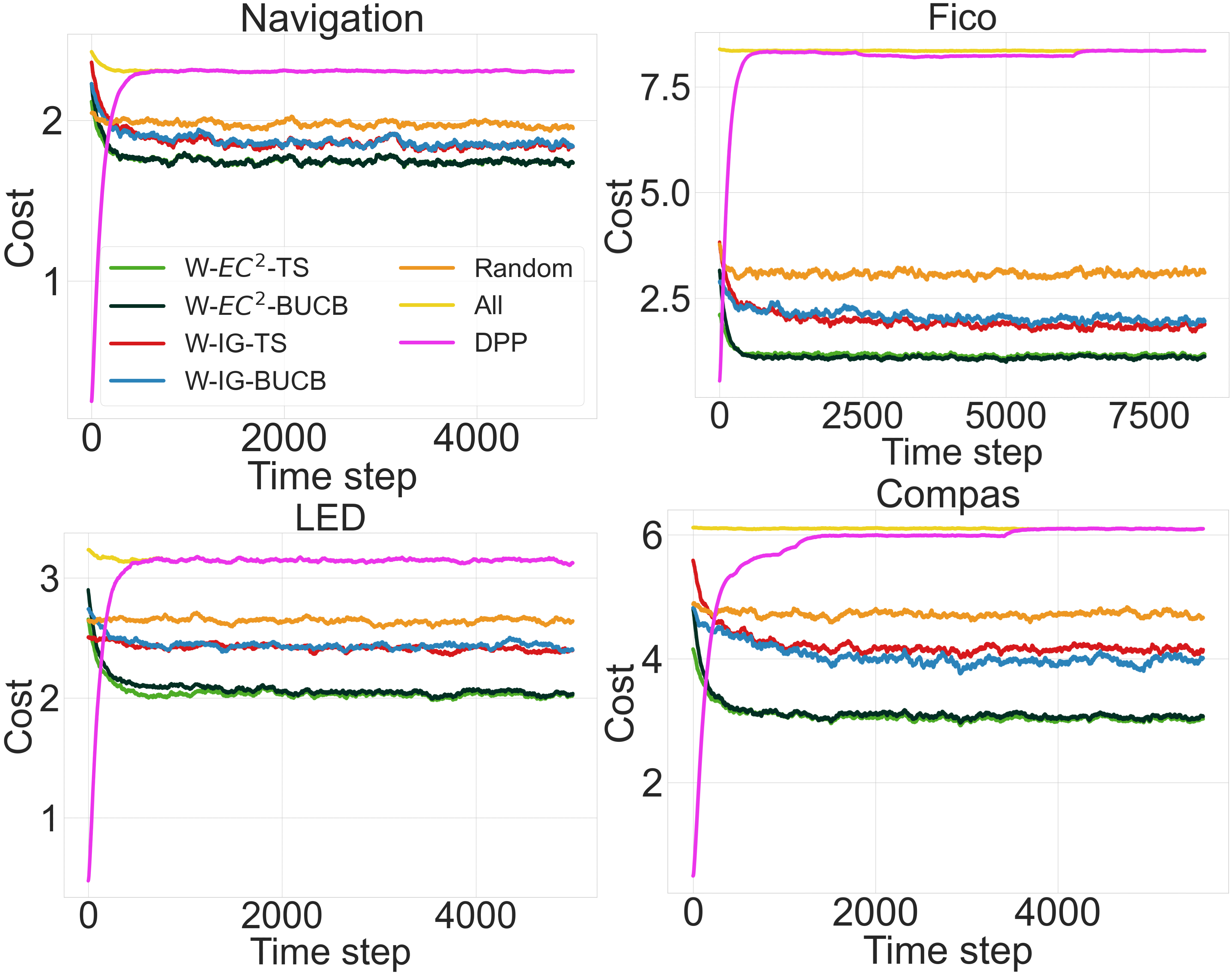
Figure 1: Decision making costs of our framework applied to four different data sets.

6 Experiments

In this section, we empirically validate our cost-efficient online decision making framework via various experiments. Unless otherwise specified, we consider Beta(2,2) as the prior distribution of all $\theta_{ij}^{*}$’s. We employ both of the cost-efficient approximate oracles introduced in Section 4.1 (W-IG and W-EC²) as the oracle in Algorithm 1. We also employ the hypothesis enumeration procedure proposed in Chen et al. (2017) to generate the most likely hypotheses for each decision region. In Appendix B, we demonstrate the applicability of our framework in the setting where the decision regions for the set of hypotheses are not known. Moreover, in Section 6.2, we provide an extension of our framework to real-valued non-binary test outcomes. We run each experiment with 5 different random seeds.

Data sets.

We apply our framework to the LED display domain data set from the UCI repository (Breiman et al., 1988). Additionally, we use the ProPublica recidivism (Compas) data set (Larson et al., 2016) and the Fair Isaac (Fico) credit risk data set (FICO et al., 2018), which both are preprocessed in the same way as by Hu et al. (2019). The aforementioned data sets contain relatively large numbers of tests and few decision outcomes, which correspond well to, e.g., the medical diagnosis example in Section 1. In applications like the charging station selection example, it might instead be reasonable to expect a large number of decision outcomes (individual charging stations or groups sharing certain characteristics) and relatively few tests (questions). Hence, in order to thoroughly evaluate the latter type of setting, we create a synthetic data set (called Navigation) with the desired characteristics. With $n=5$ tests and $m=20$ decision outcomes, we sample parameters $\theta_{ij}^{*}$ from the prior distribution Beta(2,2) for each $i\in[n]$ and $j\in[m]$, which subsequently use to generate the data set. Moreover, to demonstrate the applicability of our methods to real-valued test outcomes, we investigate the Breast Cancer Wisconsin data set (Street et al., 1993) (Section 6.2). Finally, in Section 6.3, we present the application of our framework to a real-world troubleshooting case study.

Algorithms.

In our experiments, we investigate the cost of decision making using both W-IG and W-EC² algorithms embedded in our framework (Algorithm 1). For each algorithm, we investigate both Thompson Sampling and BayesUCB for exploration. In addition to Thompson Sampling (TS) and BayesUCB (BUCB), we consider the following baselines for selecting tests in each time step:

• Random Information Acquisition. Within our framework, we can use a random subset of tests decision making. This baseline continues performing random tests until only one decision region is left (similar to W-IG and W-EC²).
  

• All. This baseline always performs all available tests, and does not consider the cost.
  

• DPP. Determinantal Point Process (DPP) provides a way to select diverse sets. With this method, we use exact sampling (Derezinski et al., 2019) (finite DPP with likelihood kernel) to subsample columns (tests). We use the implementation of Gautier et al. (2019). To perform the sampling, in each time step $t$, we provide all data points (all test results for all data points) until time $t-1$ to the sampler. The number of tests selected by the sampler is related to the number of eigenvectors of the kernel matrix.

6.1 Experimental Results

We first investigate the four data sets Navigation, LED, Fico, and Compas. As mentioned, to guarantee accurate decision regions for all hypotheses, we implement the algorithm outlined by Chen et al. (2017) for enumeration of hypotheses. In short, this algorithm produces the most probable hypotheses based on a decision and the conditional probabilities of test outcomes associated with that decision. To assign the correct decisions to hypotheses, we extract the parameter vector $\boldsymbol{\theta}$ from the entire data set and subsequently utilize the enumeration procedure to generate the most likely hypotheses for each decision. However, the parameters are not known to the agent after the enumeration of hypotheses. We assign fixed costs $\mu_{ij}^{(0)}\in[0,1]$ and $\mu_{ij}^{(1)}\in[0,1]$ (randomly sampled from a uniform distribution) for each data set before performing our experiments.

In Figure 1, we illustrate the cost of performing tests (i.e., $-\mathbb{E}[R(S^{(t)})]$) during online learning for different algorithms. The cost of each test is calculated based on Eq. 1, where the parameter $\theta_{ij}$ is derived from the data. Our results in Figure 1 show that our framework yields the lowest information acquisition cost for all data sets. DPP has a low cost initially since it only uses a few data points to perform sampling, but after a few time steps its cost becomes as high as ‘All’. Additionally, we observe that the W-EC² algorithm always has the lowest cost. This result is consistent with the theoretical results of Golovin et al. (2010) for the cost of the original EC² algorithm in the offline setting. We also observe that the exploration methods (TS and BayesUCB) exhibit very similar performances in terms of cost.

During online learning, it is observed that the cost of the random algorithm remains relatively constant, whereas the costs associated with the W-IG and W-EC² algorithms decrease until they converge to a low value. This behavior is attributed to the utilization of parameter estimates by the W-IG and W-EC² algorithms when selecting tests. As the knowledge of the agent about these parameters improves over the course of learning, the associated costs decline.

Furthermore, in Table 1, we report the average cost of decision making in a single time step for different data sets. It is obvious that our framework incurs significantly lower costs for performing tests.

6.2 Extension to Real-Valued Test Outcomes

In this section, we extend our experimental results to real-valued (non-binary) test outcomes. For this purpose, we adapt the discretization method proposed by Rahbar et al. (2023). Specifically, for each test, we consider different thresholds for “binarization”. Then, in each time step, we can calculate the gain ($\Delta_{\text{W-IG}}$ or $\Delta_{\text{W-EC}^{2}}$) for the tests using different binarization thresholds and choose the one with a maximal gain. We employ this method on the Breast Cancer Wisconsin data set. In this data set, we predict the diagnosis from 30 real-valued medical tests computed from an image of a fine needle aspirate. Figure 2 illustrates the decision making cost incurred by our framework when applied to this data set. Similar to the results depicted in Figure 1, our framework consistently achieves the lowest cost, demonstrating its effectiveness in this setting. In particular, we observe that W-EC²-TS yields the best results, and W-IG-TS, W-EC²-BUCB, and W-IG-BUCB are other suitable methods for this task.

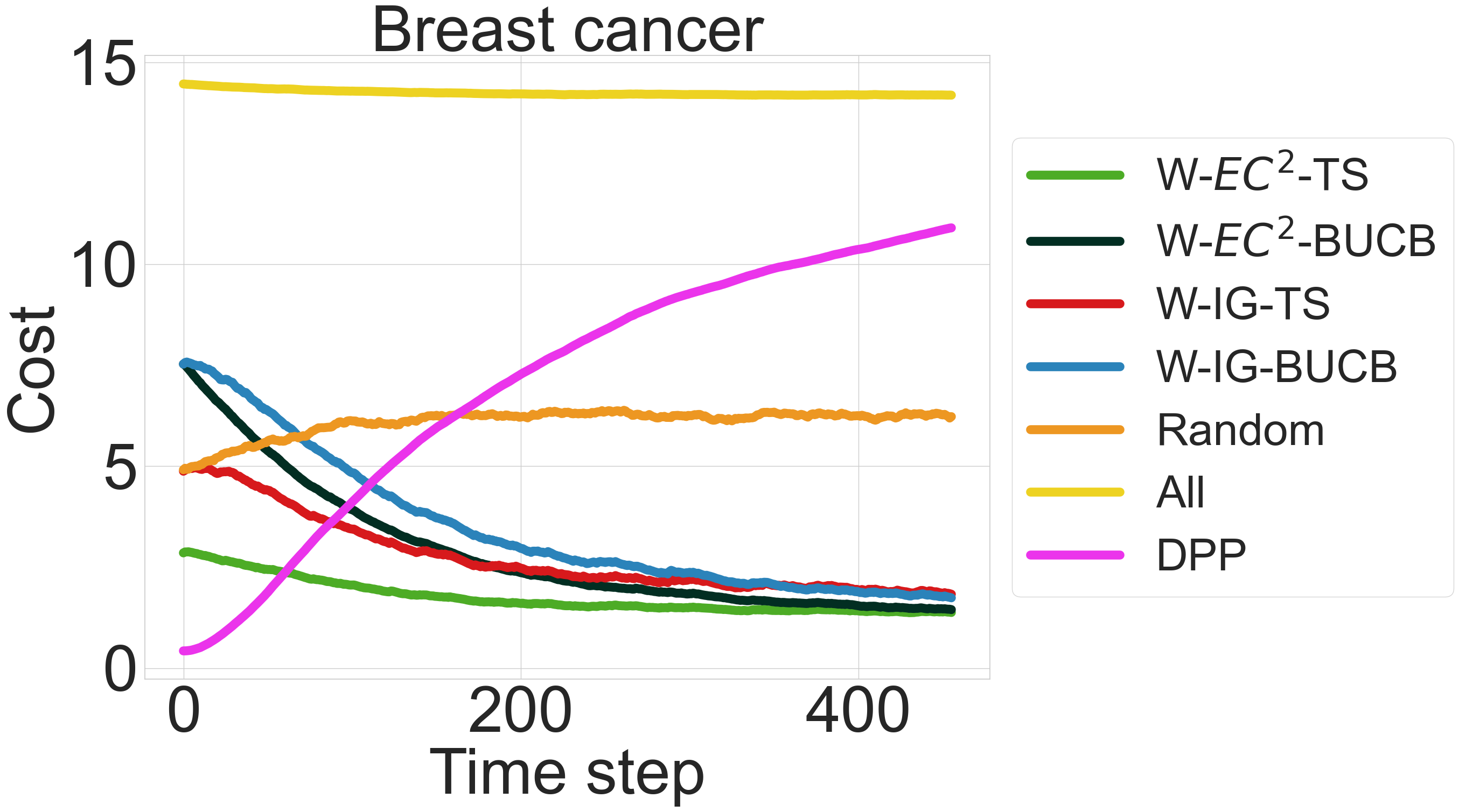
Figure 2: Decision making costs of our framework extended to real-valued test outcomes in the Breast Cancer Wisconsin data set.

6.3 Application to Online Troubleshooting

In this section, we study the application of our decision making framework for online troubleshooting. The data set for this real-world application is collected from contact center agents. The agents solve problems from mobile devices. We use a subset of this data set with 15 possible decisions and 74 tests. Each test corresponds to a symptom that a customer may or may not see on the device.

We experiment on approximately 1500 different scenarios (i.e., roughly 100 scenarios for each decision). A scenario starts with a customer entering the system. Then the online learning agent aims at finding the correct decision by asking a sequence of multiple questions of the customer (performing tests). The goal for the agent is to ask the most informative questions in a cost-efficient manner.

Figure 3 shows the cost of making decisions for different time steps (i.e., scenarios) in the same setting as Section 6.1. The results show that our framework enables the agent to find the correct decisions for troubleshooting in mobile devices with a significantly lower cost compared to other methods. Similar to previous observations, the W-EC² algorithm remains the most cost-effective method within our framework.

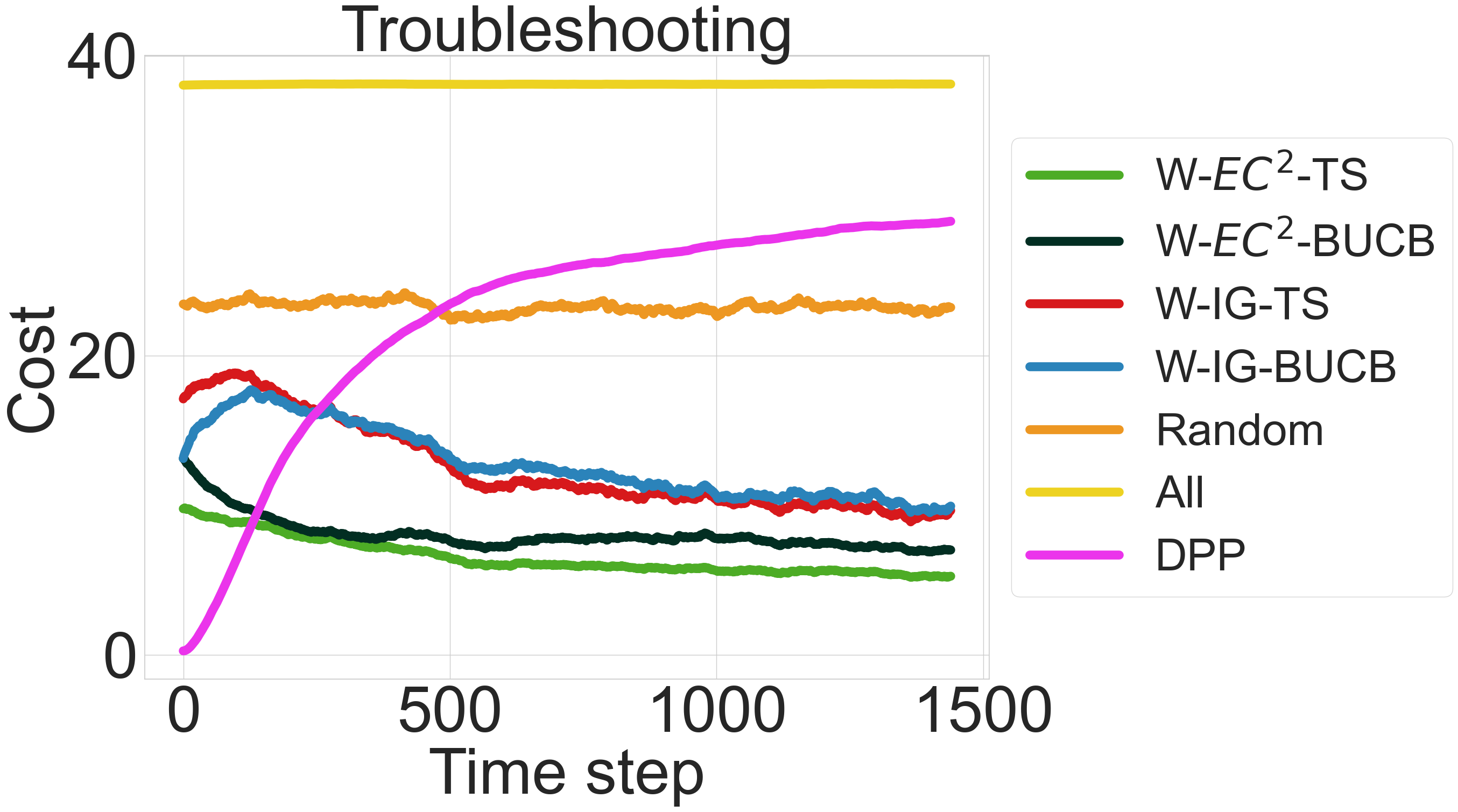
Figure 3: Decision making costs of our framework when applied to online troubleshooting.

7 Conclusion

We propose a novel framework for online decision making based on an elegant design of a combinatorial multi-armed bandit problem, which incorporates the cost of performing tests, and where the costs may be stochastic and depend on both test and decision outcomes. Within this framework, we develop various cost-efficient online decision making methods such as W-EC² and W-IG. We also adapt Thompson Sampling and BayesUCB, methods that are commonly used for exploration. In particular, we provide a theoretical upper bound for the Bayesian regret of Thompson Sampling. We finally demonstrate the performance of the framework on a number of data sets from different domains.

Appendix A Additional Proofs

A.1 Proof of Lemma 5.2

Proof.

This lemma is based on Proposition 1 of Russo and Van Roy [2014]. Given the history of played super arms (and base arms) and their rewards, we know that in Thompson Sampling the optimal super arm $S^{*,(t)}$ and the played super arm $S^{(t)}$ follow the same distribution. Since $U^{(t)}(\cdot)$ is a deterministic function, we conclude that given the history, the expected values of $U^{(t)}(S^{(t)})$ and $U^{(t)}(S^{*,(t)})$ are equal, and we have:

$$\mathbb{E}[\Delta^{(t)}_{\boldsymbol{\mu}^{*}}(S^{(t)})]=\mathbb{E}[U^{(t)}(S^{(t)})-f_{\boldsymbol{\mu}^{*}}(S^{(t)})]+\mathbb{E}[f_{\boldsymbol{\mu}^{*}}(S^{*,(t)})-U^{(t)}(S^{*,(t)})],$$

and by adding and subtracting $\mathbb{E}[L^{(t)}(S^{(t)})]$ we prove 13. ∎

A.2 Proof of Lemma 5.3

Proof.

Let $\bar{x}_{ij}^{(\tau)}$ be the average of first $\tau$ observations of $x_{i}$ under the decision region $y=j$. We have:

$$Pr\Bigg{\{}\exists t\in[T]\;\exists ij\in\mathcal{A},\big{|}\mu^{*}_{ij}-\hat{\mu}^{(t-1)}_{ij}\big{|}>\sqrt{\frac{2\log T}{N^{(t-1)}(ij)}}\Bigg{\}}$$

$$\begin{split}\stackrel{{\scriptstyle Eq.6}}{{=}}Pr\Bigg{\{}\exists t\in[T]\;\exists ij\in\mathcal{A},\big{|}\mu_{ij}^{(1)}-\mu_{ij}^{(0)}\big{|}\big{|}\theta_{ij}^{*}-\hat{\theta}_{ij}^{(t-1)}\big{|}>\sqrt{\frac{2\log T}{N^{(t-1)}(ij)}}\Bigg{\}}\end{split}$$

(since $\big{|}\mu_{ij}^{(1)}-\mu_{ij}^{(0)}\big{|}\leq 1$)

$$\leq Pr\Bigg{\{}\exists t\in[T]\;\exists ij\in\mathcal{A},\big{|}\theta_{ij}^{*}-\hat{\theta}_{ij}^{(t-1)}\big{|}>\sqrt{\frac{2\log T}{N^{(t-1)}(ij)}}\Bigg{\}}$$

(Union bound)

$$\leq\sum_{t\in[T]}\sum_{ij\in\mathcal{A}}\sum_{\tau=1}^{(t-1)}Pr\Bigg{\{}\big{|}\theta_{ij}^{*}-\bar{x}_{ij}^{(\tau)}\big{|}>\sqrt{\frac{2\log T}{\tau}}\Bigg{\}}$$

(assuming $T\geq|\mathcal{A}|$)

$$\leq T^{3}\times 2T^{-4}=\frac{2}{T}.$$

The last inequality is due to Hoeffding’s inequality (e.g., Theorem A.1 of Slivkins et al. [2019] with $\alpha=2$).

∎

A.3 Proof of Lemma 5.4

Proof.

$$\sum_{t\in[T]}\mathbb{E}[U^{(t)}(S^{(t)})-L^{(t)}(S^{(t)})]$$

$$=\sum_{t\in[T]}\mathbb{E}\Bigg{[}2\sum_{ij\in S^{(t)}}\sqrt{\frac{2\log T}{N^{(t-1)}(ij)}}\Bigg{]}$$

$$\leq\sqrt{8\log T}\sum_{t\in[T]}\mathbb{E}\Bigg{[}\sum_{ij\in S^{(t)}}\frac{1}{\sqrt{N^{(t-1)}(ij)}}\Bigg{]}$$

$$=\sqrt{8\log T}\sum_{ij\in\mathcal{A}}\mathbb{E}\Bigg{[}\sum_{t:ij\in S^{(t)}}\frac{1}{\sqrt{N^{(t-1)}(ij)}}\Bigg{]}$$

$$=\sqrt{8\log T}\sum_{ij\in\mathcal{A}}\mathbb{E}\Bigg{[}\sum_{l\in[N^{(T)}(ij)]}\frac{1}{\sqrt{l}}\Bigg{]}$$

(Lemma 1 of Russo and Van Roy 2014)

$$\leq 2\sqrt{8\log T}\sum_{ij\in\mathcal{A}}\mathbb{E}\Bigg{[}\sqrt{N^{(T)}(ij)}\Bigg{]}$$

(Cauchy–Schwarz inequality)

$$\leq 2\sqrt{8\log T}\;\mathbb{E}\Bigg{[}\sqrt{mn\sum_{ij\in\mathcal{A}}N^{(T)}(ij)}\Bigg{]}$$

$$\leq 2\sqrt{8\log T}\;\mathbb{E}\Bigg{[}\sqrt{(mn)(mn)T}\Bigg{]}$$

$$=2mn\sqrt{8T\log T}.$$

∎

Appendix B Additional Experimental Results

In this section, to demonstrate the generality of our framework, we examine the setting where the decision regions for the enumerated hypotheses are not known. This situation may lead to incorrect decisions by the agent. Specifically, in the context of online learning, our objectives are: i) to achieve highly accurate decisions, and ii) to minimize the cost of performing tests. To quantify the accuracy of the decisions, we employ a utility function. Specifically, we assign a utility of $2$ for a correct decision and $-1$ for an incorrect one. Additionally, we consider an “unknown" decision when the correct hypothesis is assigned to multiple decision regions. We define the utility of such decisions as 0.

The upper row in Figure 4 shows the cost of making decisions for different data sets (when the correct decisions of the hypotheses are not known). Similar to the findings in Figure 1, we observe that our framework (with both W-IG and W-EC²) yields a final decision with significantly lower cost than other algorithms. Again, we observe that EC² (with both Thompson Sampling and BayesUCB) has the lowest cost of performing tests. The IG algorithm results in the second lowest cost, and the random algorithm for picking tests is the third option.

As previously mentioned, when faced with unknown decision regions, our goal is to enhance the accuracy of our decisions during online learning. The lower row in Figure 4 illustrates the utility achieved by various information acquisition algorithms. Notably, our framework demonstrates comparable performance to both All and DPP in the early stages of learning. Therefore, our approach proves capable of making precise decisions with a significantly reduced cost. We note that DPP yields very low costs in the early time steps, but the corresponding utility is also very low.

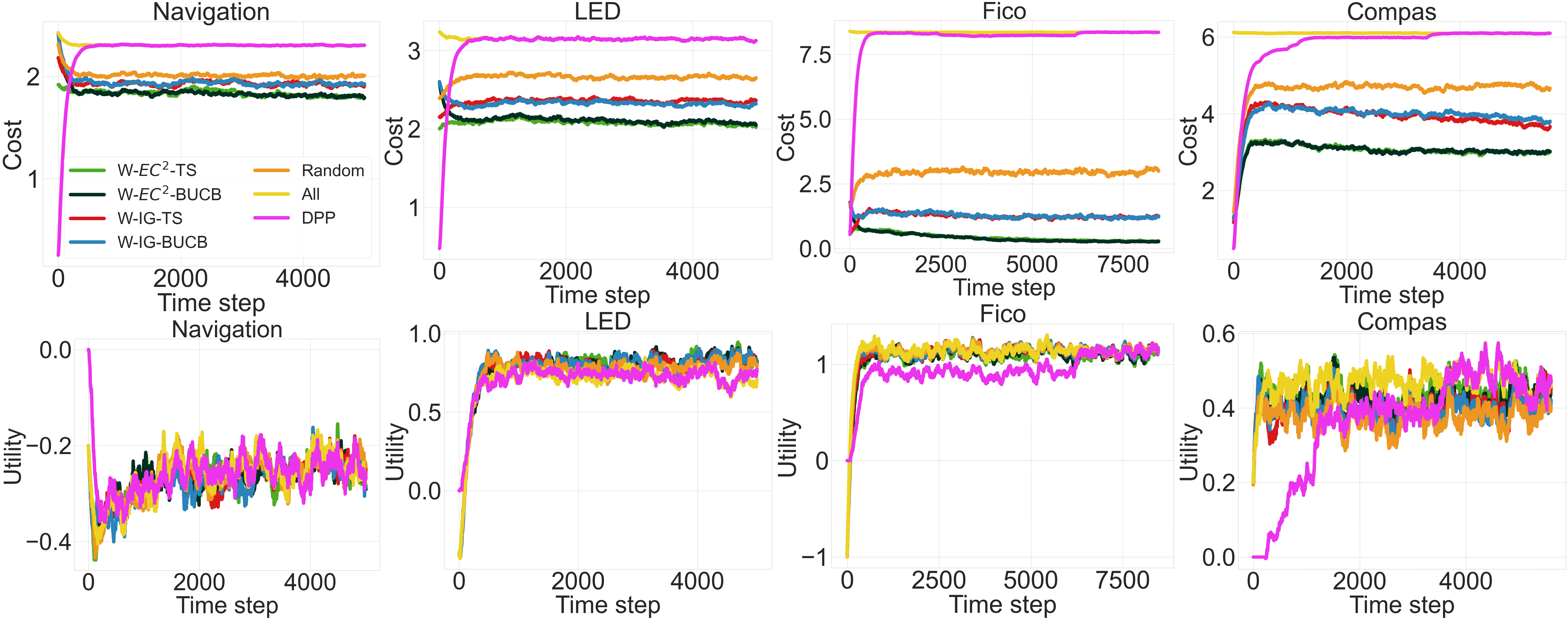
Figure 4: Decision making cost (upper row) and utility (lower row) of our framework applied to the setting that the decision regions are not known beforehand.

References

- Cesa-Bianchi and Lugosi [2012] Nicolo Cesa-Bianchi and Gábor Lugosi. Combinatorial bandits. Journal of Computer and System Sciences, 78(5):1404–1422, 2012.
- Thompson [1933] William R Thompson. On the likelihood that one unknown probability exceeds another in view of the evidence of two samples. Biometrika, 25(3/4):285–294, 1933.
- Auer et al. [2002] Peter Auer, Nicolo Cesa-Bianchi, and Paul Fischer. Finite-time analysis of the multiarmed bandit problem. Machine learning, 47:235–256, 2002.
- Golovin et al. [2010] Daniel Golovin, Andreas Krause, and Debajyoti Ray. Near-optimal bayesian active learning with noisy observations. Advances in Neural Information Processing Systems, 23, 2010.
- Dasgupta [2005] Sanjoy Dasgupta. Analysis of a greedy active learning strategy. Advances in neural information processing systems, 17:337–344, 2005.
- Kaufmann et al. [2012] Emilie Kaufmann, Olivier Cappé, and Aurélien Garivier. On bayesian upper confidence bounds for bandit problems. In Artificial intelligence and statistics, pages 592–600. PMLR, 2012.
- Zheng et al. [2012] Alice X Zheng, Irina Rish, and Alina Beygelzimer. Efficient test selection in active diagnosis via entropy approximation. arXiv preprint arXiv:1207.1418, 2012.
- Rahbar et al. [2023] Arman Rahbar, Ziyu Ye, Yuxin Chen, and Morteza Haghir Chehreghani. Efficient online decision tree learning with active feature acquisition. International Joint Conference on Artificial Intelligence (IJCAI), 32, 2023.
- Chen et al. [2017] Yuxin Chen, Jean-Michel Renders, Morteza Haghir Chehreghani, and Andreas Krause. Efficient online learning for optimizing value of information: Theory and application to interactive troubleshooting. In Proceedings of the 33rd Conference on Uncertainty in Artificial Intelligence (UAI 2017), 2017.
- Durand and Gagné [2014] Audrey Durand and Christian Gagné. Thompson sampling for combinatorial bandits and its application to online feature selection. In Workshops at the Twenty-Eighth AAAI Conference on Artificial Intelligence, 2014.
- Bouneffouf et al. [2017] Djallel Bouneffouf, Irina Rish, Guillermo A. Cecchi, and Raphaël Féraud. Context attentive bandits: Contextual bandit with restricted context. In Proceedings of the 26th International Joint Conference on Artificial Intelligence, IJCAI’17, page 1468–1475. AAAI Press, 2017. ISBN 9780999241103.
- Bouneffouf et al. [2021] Djallel Bouneffouf, Raphael Feraud, Sohini Upadhyay, Irina Rish, and Yasaman Khazaeni. Toward optimal solution for the context-attentive bandit problem. In Zhi-Hua Zhou, editor, Proceedings of the Thirtieth International Joint Conference on Artificial Intelligence, IJCAI-21, pages 3493–3500. International Joint Conferences on Artificial Intelligence Organization, 8 2021. doi:10.24963/ijcai.2021/481. URL https://doi.org/10.24963/ijcai.2021/481. Main Track.
- Åkerblom et al. [2023] Niklas Åkerblom, Fazeleh Sadat Hoseini, and Morteza Haghir Chehreghani. Online learning of network bottlenecks via minimax paths. Machine Learning, 112(1):131–150, 2023.
- Russo and Van Roy [2014] Daniel Russo and Benjamin Van Roy. Learning to optimize via posterior sampling. Mathematics of Operations Research, 39(4):1221–1243, 2014.
- Chakaravarthy et al. [2007] Venkatesan T Chakaravarthy, Vinayaka Pandit, Sambuddha Roy, Pranjal Awasthi, and Mukesh Mohania. Decision trees for entity identification: Approximation algorithms and hardness results. In Proceedings of the twenty-sixth ACM SIGMOD-SIGACT-SIGART symposium on Principles of database systems, pages 53–62, 2007.
- Breiman et al. [1988] L. Breiman, J.H. Friedman, R.A. Olshen, and C.J. Stone. LED Display Domain. UCI Machine Learning Repository, 1988.
- Larson et al. [2016] J. Larson, S. Mattu, L. Kirchner, and J. Angwin. How we analyzed the compas recidivism algorithm. SIAM journal on computing, 2016.
- FICO et al. [2018] FICO, Google, Imperial College London, MIT, University of Oxford, UC Irvine, and UC Berkeley. Explainable machine learning challenge, 2018. URL https://community.fico.com/s/explainable-machine-learning-challenge.
- Hu et al. [2019] Xiyang Hu, Cynthia Rudin, and Margo Seltzer. Optimal sparse decision trees. Advances in Neural Information Processing Systems, 32, 2019.
- Street et al. [1993] W Nick Street, William H Wolberg, and Olvi L Mangasarian. Nuclear feature extraction for breast tumor diagnosis. In Biomedical image processing and biomedical visualization, volume 1905, pages 861–870. SPIE, 1993.
- Derezinski et al. [2019] Michal Derezinski, Daniele Calandriello, and Michal Valko. Exact sampling of determinantal point processes with sublinear time preprocessing. Advances in neural information processing systems, 32, 2019.
- Gautier et al. [2019] Guillaume Gautier, Guillermo Polito, Rémi Bardenet, and Michal Valko. DPPy: DPP Sampling with Python. Journal of Machine Learning Research - Machine Learning Open Source Software (JMLR-MLOSS), 2019. URL http://jmlr.org/papers/v20/19-179.html. Code at http://github.com/guilgautier/DPPy/ Documentation at http://dppy.readthedocs.io/.
- Slivkins et al. [2019] Aleksandrs Slivkins et al. Introduction to multi-armed bandits. Foundations and Trends® in Machine Learning, 12(1-2):1–286, 2019.