Monotone Symplectic Six-Manifolds that admit a Hamiltonian GKM Action are diffeomorphic to Smooth Fano Threefolds

Abstract

Let $(M,\omega)$ be a compact symplectic manifold with a Hamiltonian GKM action of a compact torus. We formulate a positive condition on the space; this condition is satisfied if the underlying symplectic manifold is monotone. The main result of this article is that the underlying manifold of a positive Hamiltonian GKM space of dimension six is diffeomorphic to a smooth Fano threefold. We prove the main result in two steps.
In the first step, we deduce from results of Goertsches, Konstantis, and Zoller that if the complexity of the action is zero or one then the equivariant and the ordinary cohomology with integer coefficients are determined by the GKM graph. This result, in combination with a classification result by Jupp, Wall and Z̆ubr for certain six-manifolds, implies that the diffeomorphism type of a compact symplectic six-manifold with a Hamiltonian GKM action is determined by the associated GKM graph.
In the second step, based on results by Godinho and Sabatini, we compute the complete list of the GKM graphs of positive Hamiltonian GKM spaces of dimension six. We deduce that any such GKM graph is isomorphic to a GKM graph of a smooth Fano threefold.

1 Introduction

A symplectic manifold $(M,\omega)$ admits an almost complex structure $J\colon TM\rightarrow TM$, $J^{2}=-\operatorname{Id}$, that is compatible with the symplectic form $\omega$, i.e., $\omega(\cdot,J\cdot)$ is a Riemannian metric. By picking a compatible almost complex structure, we can consider the tangent bundle $TM$ as a complex vector bundle over $M$. We denote by $c_{i}(M)$ the $i$-th Chern class of $(M,\omega)$; the Chern classes are well defined since the space of compatible almost complex structures is contractible. A compact symplectic manifold $(M,\omega)$ is called monotone if $c_{1}(M)=r\cdot[\omega]$ for some $r\in\mathbb{R}$; $(M,\omega)$ is called positive monotone if $r>0$.

The algebraic counterparts of positive monotone symplectic manifolds are smooth Fano varieties. A smooth Fano variety $X$ is a compact complex manifold whose anticanonical line bundle $K_{X}^{-1}$ is ample. The ampleness of $K_{X}^{-1}$ implies that there exists a holomorphic embedding $i:X\hookrightarrow\mathbb{C}P^{N}$ such that $(K_{X}^{-1})^{k}=i^{*}\mathcal{O}(1)$ for some $N>0$ and $k>0$, known as polarisation of $X$ by $K_{X}^{-1}$. The form $i^{*}(\omega_{FS})$ is a symplectic form on $X$, where $\omega_{FS}$ is the Fubini-Study form on $\mathbb{C}P^{N}$. Moreover, the almost complex structure $J\colon TM\to TM$ induced from the complex structure on $X$ is compatible with $i^{*}(\omega_{FS})$. Since $c_{1}(X)=c_{1}(K_{X}^{-1})$ and $c_{1}(i^{*}\mathcal{O}(1))=[i^{*}(\omega_{FS})]$, the symplectic manifold $(X,i^{*}(\omega_{FS}))$ is positive monotone.

Since smooth Fano varieties carry a lot of geometric and algebraic structures it is important to understand in which content positive monotone symplectic manifolds are similar to smooth Fano varieties. In real dimensions two and four, it is known that any positive monotone symplectic manifold is diffeomorphic to a smooth Fano variety. In dimension two, this fact follows from the work of Morse [35]. In dimension four, this fact is a result of Ohta and Ono [36] based on works of Gromov [20], McDuff [31] and Taubes [39]. In dimension greater or equal to twelve, Fine and Panov [13] provide examples of positive monotone symplectic manifolds that are not diffeomorphic to a smooth Fano variety. In dimensions six, eight, and ten, the question of whether any positive monotone symplectic manifold is diffeomorphic to a Fano variety is open.

If a positive monotone symplectic manifold $(M,\omega)$ admits an integrable almost complex structure $J\colon TM\rightarrow TM$ that is compatible with $\omega$, then $M$ endowed with the complex atlas indicated by $J$ is a smooth Fano variety. This is a consequence of the Kodaira Embedding Theorem, see [32, Sect. 14.4]. In particular, if a compact symplectic manifold $(M,\omega)$ of dimension $2n$ is endowed with an effective and Hamiltonian action of a compact torus $T={(S^{1})}^{n}$ of half the dimension, then $(M,\omega)$ admits a $T$-invariant and integrable almost complex structure $J$ that is compatible with $\omega$ [9]; if $(M,\omega)$ is positive monotone, then $M$ with the induced complex atlas is a smooth Fano variety. Moreover, it is enough then that $(M,\omega)$ is monotone; a monotone symplectic manifold that admits an effective and Hamiltonian action of a compact torus is positive monotone, see [5, Proposition 3.3] and [17, Lemma 5.2]. Recall that an action of a compact torus $T={(S^{1})}^{d}$ on a symplectic manifold is Hamiltonian if there exists a moment map $\phi:M\rightarrow\mathfrak{t}^{*}$, i.e., a smooth and $T$-invariant map whose codomain is the dual of the Lie algebra $\mathfrak{t}$ of $T$ such that

$$\iota_{X^{\xi}}\omega=-\operatorname{d}\left\langle\phi,\xi\right\rangle\quad\text{for all }\,\xi\in\mathfrak{t},$$

where $X^{\xi}$ is the vector field on $M$ generated by $\xi$ and $\left\langle,\right\rangle$ is the natural pairing between $\mathfrak{t}^{*}$ and $\mathfrak{t}$. We note that on a simply connected manifold, (as is a smooth Fano variety), a smooth $T$-action is symplectic iff it is Hamiltonian: the action is symplectic iff $\iota_{X^{\xi}}\omega$ is closed for all $\xi\in\mathfrak{t}$ (by Cartan’s formula) and Hamiltonian iff $\iota_{X^{\xi}}\omega$ is exact for all $\xi\in\mathfrak{t}$. Given a connected symplectic manifold $(M,\omega)$ endowed with an effective Hamiltonian $T$-action with moment map $\phi$, we call the quadruple $(M,\omega,T,\phi)$ a Hamiltonian $\mathbf{T}$-space. Since the orbits of a Hamiltonian $T$-action on $(M,\omega)$ are isotropic, $\operatorname{dim}(T)\leq\frac{1}{2}\operatorname{dim}(M)$; we call $k:=\frac{1}{2}\operatorname{dim}(M)-\operatorname{dim}(T)$ the complexity of $(M,\omega,T,\phi)$. We also call $(M,\omega,T,\phi)$ a complexity $\mathbf{k}$ space.

The algebraic counterparts of Hamiltonian $T$-actions on symplectic manifolds are holomorphic actions of algebraic tori on compact complex manifolds. Recall that an algebraic torus $T_{\mathbb{C}}=(\mathbb{C}^{*})^{d}$ is the complexification of a compact torus $T=(S^{1})^{d}$; in particular, $T$ is contained in $T_{\mathbb{C}}$. If $X$ is a smooth Fano variety endowed with a holomorphic $T_{\mathbb{C}}$-action, then its anticanonical line bundle is $T_{\mathbb{C}}$-invariant. Hence, the polarisation of $X$ by $K_{X}^{-1}$ is $T_{\mathbb{C}}$-equivariant with respect to a $T_{\mathbb{C}}$-representation on $\mathbb{C}P^{N}$. The induced $T$-action on $\mathbb{C}P^{N}$ is Hamiltonian with respect to the Fubini-Study symplectic form $\omega_{FS}$. Hence, also the induced $T$-action on $X$ is Hamiltonian with respect to $i^{*}(\omega_{FS})$.

Since the underlying manifold of a compact monotone Hamiltonian $T$-space of complexity zero is diffeomorphic to a smooth Fano variety, it is natural to investigate the following question.

Question 1.1.

Let $(M,\omega,T,\phi)$ be a Hamiltonian $T$-space of positive complexity whose underlying symplectic manifold is monotone.

Is $M$ diffeomorphic to a smooth Fano variety?

In dimension six, i.e., the lowest dimension in which it is not known if any positive monotone symplectic manifold is diffeomorphic to a smooth Fano variety, Fine and Panov stated in [14] the following conjecture.

Conjecture 1.2.

Let $(M,\omega)$ be a monotone symplectic manifold of dimension six that admits an effective and Hamiltonian $S^{1}$-action. Then $M$ is diffeomorphic to a smooth Fano threefold.

A recent work by Lindsay and Panov [30] provides results that support this conjecture. In a series [6, 7, 8] of papers, Cho classifies monotone symplectic manifolds of dimension six admitting an effective and Hamiltonian $S^{1}$-action that is semifree. He shows that such a space admits an $S^{1}$-invariant integrable almost complex structure that is compatible with the symplectic form. Hence, Conjecture 1.2 is true if the action is in addition semifree. But it is still open if Conjecture 1.2 is true in general.

In this paper, we look at Question 1.1 in case the complexity is one.
Karshon [25] classifies compact complexity one spaces of dimension four, and shows that such a space admits an invariant compatible integrable almost complex structure. In dimension six and above, there are complexity one spaces that do not admit an invariant compatible integrable almost complex structure [40]. We note that these spaces might admit a non-invariant compatible integrable almost complex structure [19]. In any dimension, a special class of complexity one spaces, namely the tall ones, are classified by Karshon and Tolman [26, 27, 28]. Tall means that for any $x$ in the dual Lie algebra $\mathfrak{t}^{*}$ the reduced space $\phi^{-1}(x)/T$ is not a point. In [5], Sabatini, Sepe and the first author study compact monotone tall complexity one spaces, and show that in such a space the Hamiltonian action extends to an effective Hamiltonian action of complexity zero, and hence the space admits an invariant compatible integrable almost complex structure. This result is based on the classification of Karshon and Tolman. However, so far there is no classification result for non-tall Hamiltonian $T$-spaces of complexity one in dimension greater than four. Sabatini and Sepe [37] prove that a compact complexity one monotone space shares topological properties with smooth Fano varieties; namely, it is simply connected and its Todd genus is one.

The following is a special case of Conjecture 1.2.

Goal 1.3.

Let $(M,\omega,T,\phi)$ be a complexity one space where $(M,\omega)$ is a monotone symplectic manifold of dimension six. Then $M$ is diffeomorphic to a smooth Fano threefold.

By [5], this is true if the space is tall. In this article, we prove Goal 1.3 under the assumption that the $T$-action is GKM. A Hamiltonian $T$-space is GKM if the set $M^{T}$ of fixed points is finite, for each codimensional one subtorus $H\subset T$ any connected component of $M^{H}$ has at most dimension two, and the underlying manifold is compact. Note that a Hamiltonian GKM space is not tall.

We present our results in the following subsection.

1.1 Results

Given a Hamiltonian GKM space, one can associate to it canonically a graph, the so-called GKM graph; see Subsection 2.2. Moreover, any edge $e$ of the GKM graph is associated in a canonical way to a $2$-dimensional symplectic two-sphere $S_{e}$ in the underlying symplectic manifold $(M,\omega)$. We call a Hamiltonian GKM space positive if for each edge $e$ the evaluation of the first Chern class of $(M,\omega)$ on $S_{e}$ is positive. We introduce the notion of a positive Hamiltonian GKM space in a careful way at the beginning of Section 4. In particular, if the underlying symplectic manifold is monotone then the Hamiltonian GKM space is positive (see Lemma 4.6).

Theorem 1.4.

Let $(M,\omega,T,\phi)$ be a positive and six-dimensional Hamiltonian GKM space of complexity one. Then $M$ is diffeomorphic to a smooth Fano threefold.

This theorem supports Goal 1.3. Indeed a direct consequence of Theorem 1.4 and Lemma 4.6 is the following corollary.

Corollary 1.5.

Let $(M,\omega,T,\phi)$ be a Hamiltonian GKM space of complexity one where $(M,\omega)$ is a monotone symplectic manifold of dimension six. Then $M$ is diffeomorphic to a smooth Fano threefold.

We prove Theorem 1.4 in two steps.
In the first step, we relate the equivariant cohomology of a Hamiltonian GKM space of complexity one and its GKM graph, and deduce that the diffeotype of a Hamiltonian GKM space of dimension six is determined by its GKM graph. The positive condition is not needed in this step.

Theorem 1.6.

Let $(M_{1},\omega_{1},T,\phi_{1})$ and $(M_{2},\omega_{2},T,\phi_{2})$ be two Hamiltonian GKM spaces of complexity one or zero. If there exists an isomorphism from the GKM graph of $(M_{1},\omega_{1},T,\phi_{1})$ to the one of $(M_{2},\omega_{2},T,\phi_{2})$, then this isomorphism induces

• a ring isomorphism in equivariant cohomology

  $$H_{T}^{*}(M_{1};\mathbb{Z})\rightarrow H_{T}^{*}(M_{2};\mathbb{Z})$$

  that maps the equivariant Chern classes of $(M_{1},\omega_{1},T,\phi_{1})$ to the ones of $(M_{2},\omega_{2},T,\phi_{2})$ and

• a ring isomorphism in cohomology

  $$H^{*}(M_{1};\mathbb{Z})\rightarrow H^{*}(M_{2};\mathbb{Z})$$

  that maps the Chern classes of $(M_{1},\omega_{1})$ to the ones of $(M_{2},\omega_{2})$.

Theorem 1.7.

Let $(M_{1},\omega_{1},T,\phi_{1})$ and $(M_{2},\omega_{2},T,\phi_{2})$ be two Hamiltonian GKM spaces of dimension six. If there exists an isomorphism from the GKM graph of $(M_{1},\omega_{1},T,\phi_{1})$ to the one of $(M_{2},\omega_{2},T,\phi_{2})$, then there exists a (non-equivariant) diffeomorphism $M_{2}\rightarrow M_{1}$.

In [18, Theorem 3.1], Goertsches, Konstantis, and Zoller show that an isomorphism between the GKM graphs of GKM spaces, not necessarily Hamiltonian, induces a ring isomorphism in (equivariant) cohmology over $\mathbb{Z}$, assuming that the GKM spaces are compact and connected, the odd cohomolgy rings vanish, and the spaces satisfy the following technical condition: For any point $q\in M$ that does not lie in the one skeleton

$$M_{(1)}=\left\{p\in M\,|\,\dim(T\cdot p)\leq 1\right\}$$

of $M$, its stabilizer is contained in a proper subtorus of $T$. If, in addition, the GKM spaces are equipped with invariant almost complex structures and the graph-isomorphism is an isomorphism of signed GKM graphs, then the induced ring isomorphism also maps the (equivariant) Chern classes to (equivariant) Chern classes. The proof of  [18, Theorem 3.1] relies on a result of Franz and Puppe [15, Corollary 2.2]  for (not necessarily Hamiltonian) $T$-spaces. Moreover, using a classification result for compact and simply connected six-dimensional manifolds by Jupp [24], Wall [41] and Z̆ubr [42], Goertsches, Konstantis, and Zoller show that the obtained isomorphism of cohomologies is induced by a diffeomorphism between the manifolds, and hence the conclusion of Theorem 1.7 holds, if the GKM spaces are, in addition, six-dimensional and simply connected.

In Section 3, we show that the results of Goertsches, Konstantis, and Zoller imply Theorems 1.6 and 1.7. We reformulate their technical condition in terms of the weights at the fixed points, in compact Hamiltonian $T$-spaces. This formulation allows us to show that the condition holds if the complexity of the $T$-action is equal to zero or one. We deduce that Theorem 1.6 follows from [18, Theorem 3.1]. Moreover, we show that if the Hamiltonian GKM spaces are of dimension six then the conclusion of the theorem holds. Since Hamiltonian GKM spaces are simply connected (see Remark 2.17), we also deduce Theorem 1.7.
In Appendix B, we give an alternative proof of Theorem 1.6, relying on the existence of Kirwan classes that form a basis of the equivariant cohomology of a compact Hamiltonian $T$-space with isolated fixed points as a module over $H^{*}(BT;\mathbb{Z})$. We use Kirwan classes in the second step of our proof of Theorem 1.4 as well.

In the second step, we give a complete list of the GKM graphs that are coming from positive six-dimensional Hamiltonian GKM spaces. This result is based on a work by Godinho and Sabatini [16]. In [16], Godinho and Sabatini consider effective and Hamiltonian $S^{1}$-actions with only isolated fixed points on compact symplectic manifolds. They show that any such space admits a graph that describes the action and that the weights (i.e., elements of $\ell_{S^{1}}^{*}\cong\mathbb{Z}$) of the $S^{1}$-representations on the tangent spaces at the fixed points satisfy certain linear relations with respect to the graph. Note that such a graph is not unique. If the action extends to an effective and Hamiltonian $T$-action that is GKM, then the GKM graph of the corresponding Hamiltonian GKM space naturally provides a graph that describes the $S^{1}$-action. Note that the GKM graph is unique. In the GKM case, the weights (i.e., elements in $\ell_{T}^{*}\cong\mathbb{Z}^{d}$) of the $T$-representations on the tangent spaces at the fixed points also satisfy these linear relations. Furthermore, the GKM condition imposes additional constraints on the weights. In Subsection 5.2, we analyze these linear relations and constraints. For that we introduce GKM skeletons. A GKM skeleton is an $n$-valent simple graph together with an integer label for each edge. In particular, we show how an (abstract) GKM graph can be constructed from a GKM skeleton, and we discuss the uniqueness of such an (abstract) GKM graph. Note that any (abstract) GKM graph can be constructed from a GKM skeleton.
Moreover, let $(M,\omega,T,\phi)$ be a positive Hamiltonian GKM space of dimension six and let $(\Gamma_{GKM},\eta)$ be its GKM graph. So, $\Gamma_{GKM}=(V_{GKM},E_{GKM})$ is a $3$-valent graph, and the weight map $\eta:E_{GKM}\rightarrow\ell_{T}^{*}$ assigns each edge in the set $E_{GKM}$ to an element in the dual lattice of the torus $T$. By the work of Godinho and Sabatini [16], the cardinality of the vertex set $V_{GKM}$ is at most 16. In particular, there are only finitely many GKM skeletons from which a GKM graph of a positive Hamiltonian GKM space of dimension six can be constructed. Furthermore, we use Kirwan classes to formulate a necessary condition for an abstract GKM graph to be realizable by the GKM graph of a positive Hamiltonian GKM space of dimension six.
In Section 6, we sum the results of Sections 4 and 5 to create a computer program. In this program, we utilize a classification result for $3$-valent graphs with a small number of vertices from [4]. This computer program provides a finite list of (abstract) GKM graphs that must include all GKM graphs coming from positive six-dimensional Hamiltonian GKM spaces. It turns out that each (abstract) GKM graph in this list is a GKM graph that is coming from a holomorphic GKM $T$-action on a smooth Fano threefold $X$, i.e., it is the GKM graph of a Hamiltonian GKM $T$-action on $(X,i^{*}\omega_{FS})$ that is induced from a holomorphic $T_{\mathbb{C}}$-action on $X$. (We show this directly; see also [38]).
We prove the following theorem.

Theorem 1.8.

Let $(M,\omega,T,\phi)$ be a positive six-dimensional Hamiltonian GKM space of complexity one. Then its GKM graph is isomorphic to a GKM graph that is coming from a holomorphic GKM $T$-action on a Fano threefold.

Combining Theorem 1.7 and Theorem 1.8 gives Theorem 1.4.

1.2 Structure of the Article

• We introduce notations and recall preliminary results about equivariant cohomology and Hamiltonian GKM spaces that are needed in this paper.

• We reformulate the technical condition of [18] in terms of weights at fixed points in a compact Hamiltonian $T$-space and deduce Theorems 1.6 and 1.7 from [18, Theorem 3.1].

• We introduce positive Hamiltonian GKM spaces and prove basic properties of six dimensional ones. These results are needed to compute the list of graphs associated to such spaces.

• We analyze the linear relations between the first Chern class maps and the weight maps of (abstract) GKM graphs.

• We sum up the results of Sections 4 and 5 and explain how we use computer programs to classify the GKM graphs of positive six-dimensional Hamiltonian GKM spaces. We conclude by a proof of Theorem 1.8.

• We give the complete list of GKM graphs of positive six-dimensional Hamiltonian GKM spaces that are not projections of GKM graphs coming from smooth reflexive polytopes.

• We give an alternative proof, using Kirwan classes, of Theorem 1.6.

Acknowledgments. The first author would like to thank Silvia Sabatini for drawing her attention to the question of in which content smooth Fano varieties and monotone symplectic manifolds with a Hamiltonian GKM action are different. We thank Leopold Zoller and Nikolas Wardenski for clarifying remarks. The first author began working on this project during her Ph.D. studies, which were supported by the SFB-TRR 191 grant Symplectic Structures in Geometry, Algebra and Dynamics funded by the German Research Foundation. The second author is supported by the Israel Science Foundation, grant no. 570/20.

2 Preliminaries on Equivariant Cohomology and Hamiltonian GKM Spaces

2.1 Equivariant Cohomology

Let $M$ be a topological space endowed with a continuous action of a torus $T=(S^{1})^{d}$. In the Borel model, the $T$-equivariant cohomology of $M$ is defined as follows. Let $ET$ be a contractible space on which $T$ acts freely and let $BT=ET/T$ be the classifying space of $T$. The diagonal action of $T$ on $M\times ET$ is free. $M\times_{T}ET$ denotes the orbit space. The $T$-equivariant cohomology ring of $M$ is

$$H_{T}^{*}(M;R)\colon=H^{*}(M\times_{T}ET;R),$$

where $R$ is the coefficients ring. In particular, if the $T$-action on $M$ is trivial, then

$$H_{T}^{*}(M;R)=H^{*}(M;R)\otimes H^{*}(BT;R).$$

If $T=S^{1}$, then $ES^{1}$ is the unit sphere $S^{\infty}$ in $\mathbb{C}^{\infty}$ and $BS^{1}$ is $\mathbb{C}P^{\infty}$. Hence

$$H_{S^{1}}^{*}(\left\{\operatorname{point}\right\};R)=H^{*}(\mathbb{C}P^{\infty};R)=R[x],$$

where $x$ has degree $2$. Moreover, if $T$ is a $d$-dimensional torus, then $BT$ is the $d$-times product of $\mathbb{C}P^{\infty}$, and so

$$H_{T}^{*}(\left\{\operatorname{point}\right\};R)=H^{*}(BT;R)=R[x_{1},\dots,x_{d}],$$

where $\left\{x_{1},\dots,x_{d}\right\}$ is a basis of the dual lattice $\ell_{T}^{*}$ of $T$ and $\operatorname{deg}(x_{i})=2$ for all $i=1,...,d$. If the coefficient ring is $\mathbb{Z}$ then $H^{2}(BT;\mathbb{Z})$ is equal to $\ell_{T}^{*}$ and if the coefficient ring is $\mathbb{R}$ then $H^{2}(BT;\mathbb{R})$ is equal to $\mathfrak{t}^{*}$. The projection map $M\times ET\rightarrow ET$ is $T$-equivariant, so we obtain a map

$$\pi:\,M\times_{T}ET\rightarrow BT.$$

This makes $M\times_{T}ET$ an $M$-bundle over $BT$,

$$M\overset{r}{\longrightarrow}M\times_{T}ET\overset{\pi}{\longrightarrow}BT.$$

So it induces a sequence of ring homomorphisms

$$H^{*}(BT;R)\overset{\pi^{*}}{\longrightarrow}H_{T}^{*}(M;R)\overset{r^{*}}{\longrightarrow}H^{*}(M;R).$$

The map $\pi^{*}$ gives $H_{T}^{*}(M;R)$ an $H^{*}(BT;R)$-module structure by

$$\alpha\cdot\beta=\pi^{*}(\alpha)\cup\beta$$

for $\alpha\in H^{*}(BT;R)$ and $\beta\in H_{T}^{*}(M;R)$.

2.1.1 Equivariant Chern Classes

Let $V\rightarrow M$ be a $T$-invariant vector bundle. Its equivariant Euler class $e^{T}(V)$ is the Euler class of the vector bundle

$$V\times_{T}ET\rightarrow M\times_{T}ET.$$ (2.1)

If $V\rightarrow M$ is a complex $T$-invariant vector bundle, then (2.1) is a complex vector bundle, and its $i$-th equivariant Chern class $c_{i}^{T}(V)$ is defined in the same way. These equivariant classes are mapped to the ordinary Euler class resp. ordinary Chern classes of $V\rightarrow M$ under the map

$$r^{*}:H_{T}^{*}(M;\mathbb{Z})\rightarrow H^{*}(M;\mathbb{Z})$$

induced from $r:M\rightarrow M\times_{T}ET$. In case $M$ is a point, a complex $T$-invariant vector bundle $V\rightarrow M=\{p\}$ of rank $k$ is just a complex vector space of complex dimension $k$ with a $T$-representation. Let $\alpha_{1},...,\alpha_{k}\in\ell_{T}^{*}$ be the weights of this representation, then the total equivariant Chern class of the complex vector bundle $V\rightarrow\{p\}$ is

$$c^{T}(V)=\prod_{i=1}^{k}\left(1+\alpha_{i}\right)\in H_{T}^{*}(\{p\};\mathbb{Z})\cong H^{*}(BT;\mathbb{Z}).$$

Hence, the $i$-th equivariant Chern class is

$$c_{i}^{T}(V)=\sigma_{k,i}(\alpha_{1},\dots\alpha_{k})\in H^{2i}(BT;\mathbb{Z}),$$

where $\sigma_{k,i}$ is the elementary symmetric polynomial in $k$ variables of degree $i$.

In particular, the first equivariant Chern class is $c_{1}^{T}(V)=\sum_{i=1}^{k}\alpha_{i}$ and the equivariant Euler class is $e^{T}(V)=c_{k}^{T}(V)=\prod_{i=1}^{k}\alpha_{i}$.

2.1.2 The ABBV Localization Formula

Let $M^{T}$ be the set of fixed points and assume that it is not empty. Let $F$ be one of its connected components. The inclusion map $i_{F}\colon F\rightarrow M$ is a $T$-equivariant map, so it induces a map

$$i_{F}^{*}\colon H_{T}^{*}(M;R)\rightarrow H_{T}^{*}(F;R).$$

Moreover, the map $\pi\colon M\times_{T}ET\rightarrow BT$ induces a push-forward map in equivariant cohomology

$$H_{T}^{*}(M;R)\rightarrow H^{*-\operatorname{dim}(M)}(BT;R),$$

which can be seen as integration along the fibers. So we denote it by $\int_{M}$. The following theorem, due to Atiyah-Bott [2] and Berline-Vergne [3], gives a formula for the map $\int_{M}$ in terms of the fixed point set data.

Theorem 2.1.

(ABBV Localization formula) Let $M$ be a compact oriented manifold endowed with a smooth $T$-action. For $\mu^{T}\in H_{T}^{*}(M;\mathbb{Q})$

$$\int_{M}\mu^{T}\,=\,\sum_{F\subset M^{T}}\int_{F}\dfrac{i^{*}_{F}\mu^{T}}{\text{e}^{T}(N_{F})},$$

where the sum is over all the connected components $F$ of $M^{T}$ and $\text{e}^{T}(N_{F})$ is the equivariant Euler class of the normal bundle $N_{F}\to F$.

2.2 Hamiltonian GKM Spaces

Given a $T$-action on a compact connected symplectic manifold of dimension $2n$, there exists a $T$-invariant almost complex structure $J:TM\rightarrow TM$ that is compatible with the symplectic form $\omega$; moreover, the space of $T$-invariant almost complex structures on $(M,\omega)$ is contractible (see e.g., [32, Proposition 4.1.1]). For each fixed point $p\in M^{T}$, the $T$-action induces a $T$-representation on $(T_{p}M,J_{p})\cong\mathbb{C}^{n}$. This $T$-representation splits into a direct sum of one-dimensional $T$-representations, i.e., $T_{p}M=\oplus_{i=1}^{n}L_{i}$, where $L_{i}$ is a one-dimensional $T$-representation with weight $\alpha_{p,i}\in\ell_{T}^{*}$ for $i=1,...,n$. The elements $\alpha_{p,1},...,\alpha_{p,n}$ are called the weights of the $T$-representation on $T_{p}M$. These weights do not depend on the choice of such an almost complex structure since the space of $T$-invariant almost complex structures on $(M,\omega)$ is contractible. Hence, the weights are well-defined. Since the $T$-action on $M$ is effective, the following lemma holds.

Lemma 2.2.

Given an effective $T$-action on a connected symplectic $(M,\omega)$, let $p\in M^{T}$ be a fixed point and let $\alpha_{p,1},...,\alpha_{p,n}\in\ell_{T}^{*}$ be the weights of the $T$-representation on $T_{p}M$. Then the $\mathbb{Z}$-span

$$\left\{\kappa_{1}\cdot\alpha_{p,1}+\dots+\kappa_{n}\cdot\alpha_{p,n}\,|\,\kappa_{1},...,\kappa_{n}\in\mathbb{Z}\right\}$$

of the weights $\alpha_{p,1},...,\alpha_{p,n}$ is equal to $\ell_{T}^{*}$.

Proof.

Since $T$ is compact there exist $T$-invariant neighborhoods $U$ resp. $V$ of $\mathbf{0}$ in $T_{p}M$ resp. of $p$ in $M$ that are $T$-equivariantly diffeomorphic. Since the $T$-action on $M$ is effective and $M$ is connected, by the Principal Orbit Theorem [11, Theorem 2.8.5], the $T$-action on $V$ is effective. Hence, the $T$-action on $U$ is also effective. The $T$-action on $U$ is determined by the $T$-representation on $T_{p}M$ and is effective if and only if the $\mathbb{Z}$-span of the weights $\alpha_{p,1},...,\alpha_{p,n}$ is equal to $\ell_{T}^{*}$. ∎

Definition 2.3.

A Hamiltonian GKM space is a compact Hamiltonian $T$-space $(M,\omega,T,\phi)$ such that the following hold.

• The set $M^{T}$ of fixed points of the $T$-action on $M$ is finite.

• For each $p\in M^{T}$, the weights $\alpha_{p,1},...,\alpha_{p,n}\in\ell_{T}^{*}$ of the $T$-representation on $T_{p}M$ are pairwise linearly independent.

We say that the Hamiltonian $T$-action is GKM.

In the following lemma, we point out an obstruction for the dimension of the torus of a Hamiltonian GKM space.

Lemma 2.4.

Let $(M,\omega,T,\phi)$ be a Hamiltonian GKM space of dimension $2n\geq 4$. Then the dimension of the torus $T$ is greater or equal to $2$.

Proof.

Since $M$ is compact, the set of fixed points $M^{T}$ is not empty. Let $p\in M^{T}$ be a fixed point and let $\alpha_{p,1},...,\alpha_{p,n}\in\ell_{T}^{*}$ be the weights of the $T$-representation on $T_{p}M$. Since, by (ii) of Definition 2.3, these weights are pairwise linearly independent, the dimension of the torus must be greater or equal to two. ∎

Given a Hamiltonian GKM space $(M,\omega,T,\phi)$, the second condition of Definition 2.3 implies that for each codimensional one subtorus $H$ of $T$, any connected component of

$$M^{H}:=\left\{p\in M\,\mid\,t\cdot p=p\,\text{ for all }t\in H\right\}$$

has at most dimension two. Let $S$ be a two-dimensional component of $M^{H}$. Then $S$ is a symplectic embedded two-sphere and there exist exactly two points $p,q\in M^{T}$ such that $S\cap M^{T}=\{p,q\}$. Moreover, the inclusion $H\hookrightarrow T$ induces an $H$-representation on $T_{p}M$ and the tangent $T_{p}S$ is equal to the subspace of $T_{p}M$ that is fixed by the $H$-representation. Hence, there exists an element $\alpha\in\ell_{T}^{*}$ that is a weight of the $T$-representation on $T_{p}M$ such that

$$H=\exp(\operatorname{ker}\,\alpha),$$ (2.2)

where $\exp:\mathfrak{t}\rightarrow T$ is the exponential map and

$$\operatorname{ker}\,\alpha=\left\{\xi\in\mathfrak{t}\,|\,\left\langle\alpha,\xi\right\rangle=0\right\},$$

where $\left\langle,\right\rangle$ is the natural pairing between $\mathfrak{t}^{*}$ and $\mathfrak{t}$. Vice versa, $-\alpha$ is a weight of the $T$-representation on $T_{q}M$. Given $p,q\in M^{T}$ there exists at most one two-sphere $S$ that is fixed by a codimensional one subtorus such that $S\cap M^{T}=\{p,q\}$. This is since a point fixed by two different codimensional one subtori is in $M^{T}$. On the other hand, for $p\in M^{T}$ and a weight $\alpha$ of the $T$-representation on $T_{p}M$, there is a codimensional one subtorus $H$ such that the connected component of $M^{H}$ that contains $p$ is a symplectic embedded two-sphere $S$ and the weight of the $T$-representation on $T_{p}S$ is $\alpha$; moreover, the subtorus $H$ must be as in (2.2), so this sphere is unique.
The information about the $T$-representations on the tangent spaces of the fixed points and about the two-dimensional components fixed by a codimensional one subtorus can be stored in a graph, the so-called GKM graph, which is defined as follows.

Definition 2.5.

Let $(M,\omega,T,\phi)$ be a Hamiltonian GKM space. Its GKM graph $(\Gamma_{GKM},\eta)$ is the graph $\Gamma_{GKM}=(V_{GKM},E_{GKM})$ with directed edges together with the map $\eta:E_{GKM}\rightarrow\ell_{T}^{*}$ defined as follows.

• The set of vertices $V_{GKM}$ is equal to the set of fixed points $M^{T}$.

• The set of edges is a subset of $V_{GKM}\times V_{GKM}$. There exists a directed edge

  $$e=(p,q)\in V_{GKM}\times V_{GKM}$$

  if and only if there exists a two-sphere $S$ that is fixed by a codimensional one subtorus $H$ of $T$ such that $S\cap M^{T}=\{p,q\}$.

• For each edge $e=(p,q)\in E_{GKM}$, we denote by $S_{(p,q)}$ the unique two-sphere as described in $(ii)$. Then $\eta(p,q)$ is the weight of the $T$-representation on $T_{p}S_{(p,q)}$.

In the following remark, we sum up some properties of GKM graphs.

Remark 2.6.

Let $(\Gamma_{GKM},\eta)$ be the GKM graph of a Hamiltonian GKM space $(M,\omega,T,\phi)$, then the following properties hold.

• Let $2n$ be the dimension of $M$. Then the graph $\Gamma_{GKM}=(M^{T},E_{GKM})$ is $n$-valent, i.e., for each $p\in M^{T}$ there exist exactly $n$ points $p_{1},\dots,p_{n}\in M^{T}\setminus\{p\}$ such that $(p,p_{i})\in E_{GKM}$ for $i=1,...,n$. Moreover, $\eta(p,p_{1}),...,\eta(p,p_{n})$ are the weights of the $T$-representation on $T_{p}M$.

• Given $p,q\in M^{T}$, then $(p,q)$ belongs to $E_{GKM}$ if and only if $(q,p)$ belongs to $E_{GKM}$. If $(p,q)\in E_{GKM}$, then $\eta(q,p)=-\eta(p,q)$.

Definition 2.7.

Given two Hamiltonian GKM spaces $(M_{1},\omega_{1},T,\phi_{1})$ and $(M_{2},\omega_{2},T,\phi_{2})$ of the same dimension, let $(\Gamma_{1,GKM},\eta_{1})$ and $(\Gamma_{2,GKM},\eta_{2})$ be their GKM graphs. An isomorphism between these GKM graphs is a pair $(F,\theta)$ such that

• $F$ is an isomorphism between the underlying graphs

  $$\Gamma_{1,GKM}=(M_{1}^{T},E_{1,GKM})\quad\text{and}\quad\Gamma_{2,GKM}=(M_{2}^{T},E_{2,GKM}),$$

  i.e., $F:M_{1}^{T}\rightarrow M_{2}^{T}$ is a bijection such that for any two points $p,q\in M_{1}^{T}$

  $$(p,q)\in E_{1,GMK}\quad\text{if and only if}\quad(F(p),F(q))\in E_{2,GKM},$$

• $\theta:\ell_{T}^{*}\rightarrow\ell_{T}^{*}$ is a linear isomorphism such that

  $$\theta\left(\eta_{1}(p,q)\right)=\eta_{2}(F(p),F(q)),$$

  for all $(p,q)\in E_{GKM}$.

Given a Hamiltonian GKM space $(M,\omega,T,\phi)$, let $(\Gamma_{GKM},\eta)$ be its GKM graph. The initial map $i:E_{GKM}\rightarrow V_{GKM}$ and the terminal map $t:E_{GKM}\rightarrow V_{GKM}$ are given by

$$i(p,q)=p\quad\text{and}\quad t(p,q)=q\quad\text{for every edge }e=(p,q)\in E_{GKM}.$$

We associate to each point $p\in M^{T}=V_{GKM}$ the following two subsets of $E_{GKM}$,

$$E_{GKM}^{p,i}:=\{e\in E_{GKM}\mid i(e)=p\}\quad\quad\text{and}\quad\quad E_{GKM}^{p,t}:=\{e\in E_{GKM}\mid t(e)=p\}.$$

A connection along an edge $e=(p,q)\in E_{GKM}$ is a bijection

$$\nabla_{e}:E_{GKM}^{p,i}\longrightarrow E_{GKM}^{q,i}$$

such that $\nabla_{e}(p,q)=(q,p)$. The connection is compatible if for all $e^{\prime}\in E_{GKM}^{p,i}$ there exists an integer $a_{e,e^{\prime}}\in\mathbb{Z}$, such that

$$\eta(e^{\prime})-\eta(\nabla_{e}(e^{\prime}))=a_{e,e^{\prime}}\cdot\eta(e).$$

Due to the next lemma, there always exists a compatible connection.

Lemma 2.8.

Let $(M,\omega,T,\phi)$ be a Hamiltonian GKM space and let $(\Gamma_{GKM},\eta)$ be its GKM graph. For each edge $e\in E_{GKM}$ of $\Gamma_{GKM}$, there exists a connection along $e$ that is compatible.

This lemma is by [23, Theorem 1.1.2].

Remark 2.9.

Let $(M,\omega,T,\phi)$ be a Hamiltonian GKM space. Its GKM graph does not depend on the moment map $\phi$. Moreover, if $\lambda\in\mathbb{R}$ is non-zero, then the $T$-action on $(M,\lambda\cdot\omega)$ is also Hamiltonian and GKM and $\phi^{\prime}=\lambda\cdot\phi$ is a moment map. If $\lambda>0$, then the GKM graphs of $(M,\omega,T,\phi)$ and $(M,\lambda\cdot\omega,T,\lambda\cdot\phi)$ are the same.

Remark 2.10.

Let $(M,\omega,T,\phi)$ be a Hamiltonian GKM space and let $(\Gamma_{GKM},\eta)$ be its GKM graph. Let $e=(p,q)\in E_{GKM}$ be an edge. The moment map images $\phi(p)$ and $\phi(q)$ determine $\eta(p,q)$ up to positive integer multiple. Namely, let $S$ be the unique two-sphere in $M$ that is fixed by a codimensional one subtorus of $T$ such that $S\cap M^{T}=\{p,q\}$. The moment map image $\phi(S)$ is given by the compact line segment through $\phi(p)$ and $\phi(q)$ in the vector space $\mathfrak{t}^{*}$. This line segment is rational, i.e., there exists a unique primitive vector $\alpha\in\ell_{T}^{*}\setminus\{0\}\subset\mathfrak{t}^{*}\setminus\{0\}$ such that $\phi(q)-\phi(p)=r\cdot\alpha$ for some real number $r>0$. In particular,

$$\eta(p,q)=m\cdot\alpha\quad\text{for some positive integer }m.$$

2.2.1 GKM Graphs of Symplectic Toric Manifolds

By the famous Convexity Theorem of Atiyah [1] and Guillemin-Sternberg [22], the moment map image of a compact Hamiltonian $T$-space is a convex polytope. So the moment map image is called the moment map polytope. Moreover, compact symplectic toric manifolds, i.e., compact complexity zero spaces, are determined by their moment map polytopes (up to isomorphism) and the moment map polytope of such a space is smooth [9]. We recall this and the definition of smooth polytopes in the following.

Definition 2.11.

Let $\Delta$ be a $d$-dimensional polytope in $\mathbb{R}^{d}$. A vertex $v$ of $\Delta$ is called smooth if there exist exactly $d$ edges of $\Delta$ that contain $v$ and a $\mathbb{Z}$-basis $\alpha_{v,1},...,\alpha_{v,d}$ of $\mathbb{Z}^{d}$ such that the edges that contain $v$ are given by

$$\left(v+\mathbb{R}_{\geq 0}\cdot\alpha_{v,j}\right)\cap\Delta$$

for $j=1,...,d$. The polytope $\Delta$ is called smooth if all of its vertices are smooth.

Remark 2.12.

Let $T$ be a $d$-dimensional torus. By considering its dual Lie algebra $\mathfrak{t}^{*}\cong\mathbb{R}^{d}$ together with the dual lattice $\ell^{*}_{T}\cong\mathbb{Z}^{d}$, the definition of smooth polytopes in $\mathbb{R}^{d}$ naturally extends to polytopes in $\mathfrak{t}^{*}$.

Theorem 2.13.

[9, Delzant] Let $(M,\omega,T,\phi)$ be a compact symplectic toric manifold. The space admits an integrable almost complex structure that is T-invariant and compatible with $\omega$ and the moment map polytope is a smooth polytope. Moreover, if $\Delta$ is a smooth polytope in $\mathfrak{t}^{*}$, then there exists a unique (up to isomorphism) compact symplectic toric manifold whose moment map image is $\Delta$.

Let $(M,\omega,T,\phi)$ be a compact symplectic toric manifold. Then the space is also GKM and its GKM graph $(\Gamma_{GKM},\eta)$ is determined by the moment map polytope $\Delta_{M}\colon=\phi(M)$, as follows. The moment map induces a bijection from the set of fixed points to the set of vertices of $\Delta_{M}$. Hence, the set $V_{GKM}$ of vertices of the graph $\Gamma_{GKM}$ can be identified with the set of vertices of the polytope $\Delta_{M}$. There exists an edge $(p,q)\in E_{GKM}\subset M^{T}\times M^{T}$ if and only if the corresponding vertices $\phi(p)$ and $\phi(q)$ of $\Delta_{M}$ are connected by an edge of the polytope $\Delta_{M}$. If $(p,q)\in E_{GKM}$, then $\eta(p,q)$ is the unique primitive element in $\ell_{T}^{*}$ such that $\phi(q)-\phi(p)=r\cdot\eta(p,q)$ for some $r>0$. In the following, we say that the GKM graph of a compact symplectic toric manifold $(M,\omega,T,\phi)$ is coming from the smooth polytope $\Delta_{M}\colon=\phi(M)$. We note that the GKM graph does not determine the moment map polytope. In particular, the GKM graph does not contain information about the symplectic form.

Example 2.14.

In Figure 1, the polytopes (A), (B) and (C) are smooth.

• The polytope (A) is the moment map polytope of the standard $(S^{1})^{2}$-action on $(\mathbb{C}P^{2},\omega_{FS})$.

• The polytope (B) is the moment map polytope of the standard $(S^{1})^{2}$-action on $(S^{2}\times S^{2},\omega\oplus\omega)$, where $\omega$ is volume form on $S^{2}$ with $\int_{S^{2}}\omega=2$.

• The polytope (C) is the moment map polytope of the standard $(S^{1})^{2}$-action on $(S^{2}\times S^{2},\omega\oplus\frac{5}{4}\omega)$.

The polytopes (A) and (B) induce the same GKM graph.

Definition 2.15.

Let $\Delta$ be a $d$-dimensional polytope in $\mathbb{R}^{d}$ that is integral, i.e., all of its vertices lie in $\mathbb{Z}^{d}$. For each facet $F$ of $\Delta$, let $l_{F}\in\mathbb{Z}^{d}$ be the primitive outward normal vector to the hyperplane defining $F$, i.e.,

$$F=\left\{x\in\mathbb{R}^{d}\,|\,\left\langle l_{F},x\right\rangle_{\mathbb{R}^{d}}=c_{F}\right\}\cap\Delta\quad\text{and}\quad\Delta\subseteq\left\{x\in\mathbb{R}^{d}\,|\,\left\langle l_{F},x\right\rangle_{\mathbb{R}^{d}}\leq c_{F}\right\}$$

for some $c_{F}\in\mathbb{R}$, where $\left\langle,\right\rangle_{\mathbb{R}^{d}}$ is the standard scalar product on $\mathbb{R}^{d}$. The polytope $\Delta$ is reflexive if $c_{F}=1$ for any facet $F$ of $\Delta$.

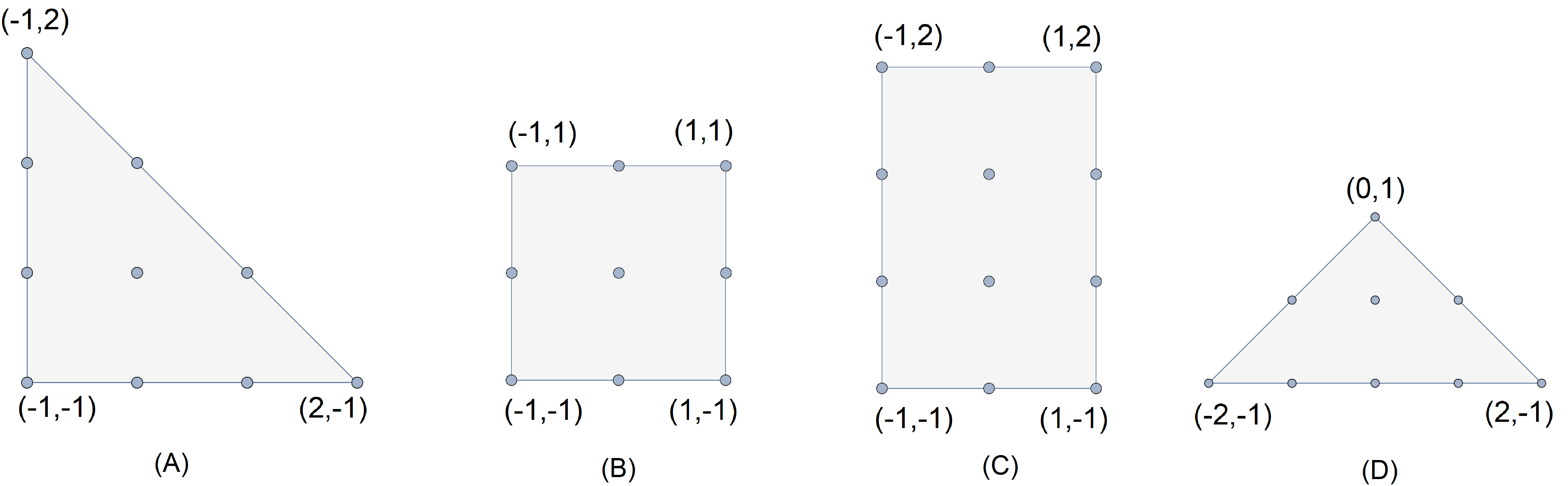
Figure 1: The polytopes (A) and (B) are smooth and reflexive. The polytope (C) is smooth, but not reflexive. The polytope (D) is reflexive, but not smooth.

Monotone symplectic toric manifolds and reflexive polytopes are related as follows.

Proposition 2.16.

Let $\Delta$ be a smooth polytope in $\mathfrak{t}^{*}$ and let $(M,\omega,T,\phi)$ the compact symplectic toric manifold whose moment map image is $\Delta$. Then the following two conditions are equivalent.

• There exists $\nu\in\mathfrak{t}^{*}$ such that $\Delta+\nu$ is reflexive.

• $(M,\omega)$ is monotone with $c_{1}(M)=[\omega]$.

A proof of this proposition can be found in [12, Proposition 1.8] and [33, Sect.3]

2.2.2 Projections of GKM Graphs

Given a Hamiltonian GKM space $(M,\omega,T,\phi)$, let $T^{\prime}$ be a subtorus of $T$. The restriction of the $T$-action to $T^{\prime}$ is again a Hamiltonian action on $(M,\omega)$ with moment map

$$i^{*}\circ\phi:M\rightarrow(\mathfrak{t^{\prime}})^{*},$$

where $i^{*}:\mathfrak{t}^{*}\rightarrow(\mathfrak{t}^{\prime})^{*}$ is the dual of the inclusion $i:\mathfrak{t}^{\prime}\hookrightarrow\mathfrak{t}$ from the Lie algebra of $T^{\prime}$ to the one of $T$. So the quadruple

$$(M,\omega,T^{\prime},i^{*}\circ\phi)$$

is a compact Hamiltonian $T$-space. The map $i^{*}$ maps the dual lattice $\ell_{T}^{*}$ of $T$ to the dual lattice $\ell_{T^{\prime}}^{*}$ of $T^{\prime}$. Note that the quadruple is a Hamiltonian GKM space if and only if for each fixed point $p\in M^{T}$, the weights of the $T$-representation on $T_{p}M$ are mapped to pairwise linearly independent weights. In this case the GKM graph of $(M,\omega,T^{\prime},i^{*}\circ\phi)$ is $(\Gamma_{GKM},i^{*}\circ\eta)$, where $(\Gamma_{GKM},\eta)$ is the GKM graph of $(M,\omega,T,\phi)$. We say that the GKM graph $(\Gamma_{GKM},i^{*}\circ\eta)$ is a projection of $(\Gamma_{GKM},\eta)$.

2.3 Compact Hamiltonian $T$-spaces with only Isolated Fixed Points

2.3.1 Generic Vectors and Morse Theory

Let $(M,\omega,T,\phi)$ be a compact Hamiltonian $T$-space with only isolated fixed points. A vector $\xi\in\mathfrak{t}$ is called generic if $\left\langle\alpha,\xi\right\rangle\neq 0$ for each weight $\alpha\in\ell_{T}^{*}$ of the $T$-representation of $T_{p}M$ for every $p\in M^{T}$. If $\xi\in\mathfrak{t}$ is generic, then the $\xi$-component of the moment map

$$\phi^{\xi}:M\rightarrow\mathbb{R}\,,\quad p\mapsto\left\langle\phi(p),\xi\right\rangle$$

is a Morse function and its set of critical points coincides with the set of fixed points $M^{T}$.

Given $p\in M^{T}$, the Morse index of $p$ with respect to $\phi^{\xi}$ is equal to twice the number of weights of the $T$-representation on $T_{p}M$ that satisfy $\left\langle\alpha,\xi\right\rangle<0$.

For any fixed point $p\in M^{T}$ we define the index $\lambda(p)$ of $p$ with respect to $\xi$ as follows.

$$\lambda(p)\,\text{equals half of the Morse index of }p\,\text{with respect to }\phi^{\xi},$$

or equivalently,

$\lambda(p)$ is the number of weights of the $T$-representation on $T_{p}M$ that satisfy $\left\langle\alpha,\xi\right\rangle<0.$

Remark 2.17.

In a Hamiltonian $T$-space with only isolated fixed points, for each $p\in M^{T}$ its Morse index with respect to $\phi^{\xi}$ (for a generic vector $\xi$) is even. Hence, if $M$ is also compact, it is homotopy equivalent to a CW complex with only even cells. This implies that $M$ is simply connected, $H^{\operatorname{odd}}(M;\mathbb{Z})=0$ and the odd Betti numbers of $M$ are zero.

Remark 2.18.

Assume that $(M,\omega,T,\phi)$ is a Hamiltonian GKM space and let $(\Gamma_{GKM},\eta)$ be its GKM graph. Given a fixed point $p\in M^{T}$, let $p_{1},\dots,p_{n}\in M^{T}\setminus\{p\}$ be the unique fixed points such that $(p,p_{i})\in E_{GKM}$. Since $\eta(p,p_{1}),...,\eta(p,p_{n})$ are the weights of the $T$-representation on $T_{p}M$, we have that $\lambda(p)$ is equal to the number of edges of $(p,p_{1}),...,(p,p_{n})$ that satisfy

$$\phi^{\xi}(p_{i})<\phi^{\xi}(p),\,\text{or equivalently, }\,\left\langle\eta(p,p_{i}),\xi\right\rangle<0.$$

Remark 2.19.

Note that since the underlying manifold of a Hamiltonian GKM space is connected, its GKM graph $(\Gamma_{GKM},\eta)$ is also connected. The latter means that for two different points $p,q\in M^{T}$, there exists a sequence $p_{0},...,p_{k}\in M^{T}$ such that $p_{0}=p$, $p_{k}=q$ and $(p_{i},p_{i+1})\in E_{GKM}$ for $i=0,\dots,k-1$. We say that $p$ and $q$ are connected by a path. To see this fix a generic vector $\xi\in\mathfrak{t}$ and let $p_{min}$ be the unique fixed point on which $\phi^{\xi}$ attains its minimum. Let $p\in M^{T}\setminus\{p_{min}\}$ be another fixed point. We set $p_{0}=p$. By Remark 2.18 there exists a fixed point $p_{1}\in M^{T}\setminus\{p_{0}\}$ with $\phi^{\xi}(p_{1})<\phi^{\xi}(p_{0})$. It might be that $p_{1}=p_{min}$; otherwise, we repeat this step. Note that since $M^{T}$ is finite, we conclude that there exist $p_{0},...,p_{k}$ such that $p_{0}=p$, $p_{k}=p_{min}$ and $(p_{i},p_{i+1})\in E_{GKM}$ for $i=0,\dots,k-1$. Hence, each $p\in M^{T}\setminus\{p_{min}\}$ is connected with $p_{min}$. Moreover, since $(p,q)\in E_{GKM}$ implies $(q,p)\in E_{GKM}$, it follows that any two fixed points are connected by a path.

2.3.2 Kirwan Classes

Let $(M,\omega,T,\phi)$ be a compact Hamiltonian $T$-space with only isolated fixed points. By the Kirwan Injectivity Theorem [29], the inclusion $i:M^{T}\hookrightarrow M$ induces an injective map $i^{*}:H_{T}^{*}(M;\mathbb{Z})\rightarrow H_{T}^{*}(M^{T};\mathbb{Z})$. Therefore, we consider $H_{T}^{*}(M;\mathbb{Z})$ as a subring of $H_{T}^{*}(M^{T};\mathbb{Z})$. Since $H^{*}_{T}(\{p\};\mathbb{Z})\cong H^{*}(BT;\mathbb{Z})$, we consider the ring $H_{T}^{*}(M^{T};\mathbb{Z})$ as the ring of maps from $M^{T}$ to $H^{*}(BT;\mathbb{Z})$, denoted by

$$\operatorname{Maps}\left(M^{T},H^{*}(BT;\mathbb{Z})\right).$$

So any class $\alpha\in H_{T}^{*}(M;\mathbb{Z})$ is completely determined by the restrictions

$$i^{*}_{\{p\}}(\alpha)\in H^{*}_{T}(\{p\};\mathbb{Z})\cong H^{*}(BT;\mathbb{Z})$$

for all $p\in M^{T}$, where $i^{*}_{\{p\}}$ is the map induced by the inclusion $p\hookrightarrow M$. For simplicity, in the following we write $\alpha(p)$ instead of $i^{*}_{\{p\}}(\alpha)$. Since we can consider $H^{*}_{T}(M;\mathbb{Z})$ as a subring of $\operatorname{Maps}\left(M^{T},H^{*}(BT;\mathbb{Z})\right)$, we have that

$$H^{2i}_{T}(M;\mathbb{Z})=H_{T}^{*}(M;\mathbb{Z})\cap\operatorname{Maps}\left(M^{T},H^{2i}(BT;\mathbb{Z})\right).$$

We use results by Kirwan [29] on the existence of so-called Kirwan classes. We repeat the definition of Kirwan classes. Let $(M,\omega,T,\phi)$ be a compact Hamiltonian $T$-space with only isolated fixed points and let $\xi\in\mathfrak{t}$ be a generic vector. For each $p\in M^{T}$ the equivariant Euler class of negative tangent bundle at $p$ with respect to $\phi^{\xi}$ is

$$\Lambda_{p}^{-}=\prod_{\begin{subarray}{c}i=1,...,n\\ \left\langle a_{p_{i}},\xi\right\rangle<0\end{subarray}}\alpha_{p,i},$$

where $\alpha_{p,1},...,\alpha_{p,n}$ are the weights of the $T$-representation on $T_{p}M$. Here, the empty product is equal to the multiplicative identity of $H^{*}(BT;\mathbb{Z})$.

Lemma 2.20.

(Kirwan [29]) Let $(M,\omega,T,\phi)$ be a compact Hamiltonian $T$-space with only isolated fixed points and let $\xi\in\mathfrak{t}$ be a generic vector. For every fixed point $p\in M^{T}$, there exists an equivariant class $\gamma_{p}\in H_{T}^{2\lambda(p)}(M;\mathbb{Z})$ such that

• $\gamma_{p}(p)=\Lambda_{p}^{-}$ and

• $\gamma_{p}(q)=0$ for every fixed point $q\in M^{T}\setminus\{p\}$ with $\phi^{\xi}(q)\leq\phi^{\xi}(p)$.

Moreover, for any choice of such classes, the set $\{\gamma_{p}\}_{p\in M^{T}}$ is a basis for $H_{T}^{*}(M;\mathbb{Z})$ as a module over $H^{*}(BT;\mathbb{Z})$.

A class that satisfies properties (i) and (ii) of Lemma 2.20 is called a Kirwan class at $p$.

In general, Kirwan classes are not unique. Let $p$ and $q$ be fixed points and let $\gamma_{p}$ and $\gamma_{q}$ be Kirwan classes at $p$ and $q$. If $\lambda(p)\leq\lambda(q)$ and $\phi^{\xi}(p)\leq\phi^{\xi}(q)$, then $\gamma_{p}+f\cdot\gamma_{q}$ is also a Kirwan class at $p$ for any $f\in H^{2(\lambda(p)-\lambda(q))}(BT;\mathbb{Z})$. In order to recover the multiplicative structure of $H_{T}^{*}(M;\mathbb{Z})$ it is enough to compute the restrictions $\gamma_{p}(q)$ for all $p,q\in M^{T}$ for some set of Kirwan classes $\{\gamma_{p}\}_{p\in M^{T}}$. In this case one can easily compute the equivariant structure constants with respect to this basis; these are, for all $q,p,r\in M^{T}$, the unique elements $c^{r}_{p,q}\in H^{*}(BT;\mathbb{Z})$ such that $\gamma_{p}\cdot\gamma_{q}=\sum_{r\in M^{T}}c^{r}_{p,q}\gamma_{r}$. Furthermore, if one knows these equivariant structure constants, then the ordinary cohomology ring is also known. Indeed, by the Kirwan Surjectivity Theorem [29], the restriction map

$$r^{*}:H_{T}^{*}(M;\mathbb{Z})\rightarrow H^{*}(M;\mathbb{Z})$$

is surjective and its kernel is the ideal generated by $H^{2}(BT;\mathbb{Z})$. If we denote by $\tau_{p}$ the image of $\gamma_{p}$ for $p\in M^{T}$, then $H^{2i}(M;\mathbb{Z})\cong\mathbb{Z}^{b_{2i}(M)}$ is the free abelian group generated by the elements $\tau_{p}$ with $\lambda(p)=i$ and $H^{odd}(M;\mathbb{Z})=0$. The multiplicative structure of $H^{*}(M;\mathbb{Z})$ is given by

$$\tau_{p}\cdot\tau_{q}=\sum_{\begin{subarray}{c}r\in M^{T}\\ \lambda(r)=\lambda(p)+\lambda(q)\end{subarray}}c_{p,q}^{r}\tau_{r}\,,$$

where the empty sum is equal to zero.

Remark 2.21.

Let $\alpha\in H_{T}^{*}(M;\mathbb{Z})$ be a class and let $\{\gamma_{p}\}_{p\in M^{T}}$ be a set of Kirwan classes. For each $p\in M^{T}$, there exists a unique element $c_{p}\in H^{*}(BT;\mathbb{Z})$ such that $\alpha=\sum_{p\in M^{T}}c_{p}\cdot\gamma_{p}$. These coefficients can be computed as follows. Given $p\in M^{T}$ and suppose that we already know $c_{q}$ for all $q\in M^{T}$ with $\phi^{\xi}(q)<\phi^{\xi}(p)$. We have

$$\alpha(p)=c_{p}\cdot\Lambda_{p}^{-}+\sum_{\begin{subarray}{c}q\in M^{T}\\ \phi^{\xi}(q)<\phi^{\xi}(p)\end{subarray}}c_{q}\cdot\gamma_{q}(p).$$ (2.3)

Since $\Lambda_{p}^{-}\neq 0$, $c_{p}$ can be simply recovered from equation (2.3).

A simple consequence of (2.3) is the following.

Lemma 2.22.

Let $(M,\omega,T,\phi)$ be a Hamiltonian $T$-space with only isolated fixed points, let $\xi\in\mathfrak{t}$ be a generic vector and let $\alpha\in H_{T}^{*}(M;\mathbb{Z})$.

• If $p$ is a fixed point such that $\alpha(q)=0$ for all $q\in M^{T}$ with $\phi^{\xi}(q)<\phi^{\xi}(p)$, then $\alpha(p)=f\cdot\Lambda_{p}^{-}$ for some $f\in H^{*}(BT;\mathbb{Z})$.

• If $\alpha\in H^{2i}_{T}(M;\mathbb{Z})$ and $\alpha(q)=0$ for all $q\in M^{T}$ with $\lambda(q)\leq i$, then $\alpha=0$.

3 The Equivariant Cohomology of a Hamiltonian GKM Space is determined by its GKM Graph

In this section, we prove the following proposition that is needed for the proof of Theorems 1.6 and 1.7 that we give at the end of this section.

Proposition 3.1.

Let $(M,\omega,T,\phi)$ be a compact Hamiltonian $T$-space of complexity zero or one. Let $p\in M$ be a point that does not lie in the one skeleton

$$M_{(1)}=\left\{q\in M\,|\,\dim(T\cdot q)\leq 1\right\}.$$

Then the stabilizer of $p$ is contained in a proper subtorus of $T$.

3.1 Subgroups of $T$ defined by subsets of $\ell_{T}^{*}$

Let $T$ be a compact $d$-dimensional torus. We identify its Lie algebra $\mathfrak{t}$ with $\mathbb{R}^{d}$. Let $\exp:\mathfrak{t}\rightarrow T$ be the exponential map. The lattice of $T$ is

$$\ell_{T}=\ker\left(\exp\right)\cong\mathbb{Z}^{d}.$$

Let $\mathfrak{t}^{*}$ be the dual Lie algebra. The dual lattice is

$$\ell_{T}^{*}=\left\{\alpha\in\mathfrak{t}^{*}\,|\,\alpha(\xi)\in\mathbb{Z}\,\text{for all }\xi\in\ell_{T}\right\}\cong\mathbb{Z}^{d}.$$

A subset $A\subset\ell_{T}^{*}$ defines a subgroup of $\mathfrak{t}$, namely

$$\mathcal{K}(A):=\left\{\xi\in\mathfrak{t}\,|\,\alpha(\xi)\in\mathbb{Z}\,\,\text{for all }\alpha\in A\right\}.$$

If $A$ is empty, we set $\mathcal{K}(A)=\mathfrak{t}$. Through the exponential map $A$ defines also a subgroup of $T$, namely $\exp\left(\mathcal{K}(A)\right)$ .

Example 3.2.

If the $\mathbb{Z}$-span of the elements of $A$ is equal to $\ell_{T}^{*}$, then $\mathcal{K}(A)$ is $\ell_{T}$ and $\exp\left(\mathcal{K}(A)\right)$ is trivial.

A vector in $\ell_{T}^{*}$ is called primitive if there exists no integer $p\geq 2$ that divides the vector in $\ell_{T}^{*}\cong\mathbb{Z}^{d}$. In particular, a primitive vector is non-zero. Let $\alpha\in\ell_{T}^{*}$ be a non-zero vector. There exist a unique primitive vector $v$ and a unique integer $k\geq 1$ such that $\alpha=k\cdot v$. Namely, $k$ is the largest integer that divides $\alpha$ in $\ell_{T}^{*}$. In particular, $\alpha$ is primitive if and only if $k=1$.

Example 3.3.

Let $\alpha\in\ell_{T}^{*}$ be a non-zero vector. Let $k\geq 1$ be the unique integer such that $\alpha=k\cdot v_{1}$, where $v_{1}\in\ell_{T}^{*}$ is primitive. Since $v_{1}$ is primitive, there exist vectors $v_{2},...,v_{d}$ such that $v_{1},...,v_{d}$ is a $\mathbb{Z}$-basis of $\ell_{T}^{*}$. Let $\xi_{1},...,\xi_{d}\in\ell_{T}$ be the dual basis, i.e., $v_{i}(\xi_{i})=1$ and $v_{i}(\xi_{j})=0$ if $i\neq j$. We have that

$$\left\{\xi\in\mathfrak{t}\,|\,\alpha(\xi)=0\right\}=\left\{\lambda_{2}\cdot\xi_{2}+...+\lambda_{d}\cdot\xi_{d}\,|\,\lambda_{2},...,\lambda_{d}\in\mathbb{R}\right\}\quad\text{and}$$

$$\mathcal{K}(\{\alpha\})=\frac{1}{k}\mathbb{Z}\cdot\xi_{1}\oplus\left\{\xi\in\mathfrak{t}\,|\,\alpha(\xi)=0\right\}.$$

If $\alpha$ is not primitive, i.e, $k\geq 2$, then $\exp\left(\mathcal{K}(\{\alpha\})\right)=Z\otimes H,$ where $Z\cong\mathbb{Z}_{k}$ is the cyclic subgroup of $T$ that is generated by $\exp\left(\frac{1}{k}\cdot\xi_{1}\right)$ and $H$ is the codimensional one subtorus of $T$ whose Lie algebra is $\left\{\xi\in\mathfrak{t}\,|\,\alpha(\xi)=0\right\}.$ If $\alpha$ is primitive, i.e., $k=1$, then $\exp\left(\mathcal{K}(\{\alpha\})\right)=H$.

Definition 3.4.

Given two vectors $\alpha_{1},\alpha_{2}\in\ell_{T}^{*}$, we say that the vectors are coprime if there exists no integer $p\in\mathbb{Z}_{\geq 2}$ that divides both vectors in $\ell_{T}^{*}$.

Remark 3.5.

Let $\alpha_{1},\alpha_{2}\in\ell_{T}^{*}$ be two vectors. If $\alpha_{1}$ is primitive, then the vectors are coprime. On the other side, if $\alpha_{1}$ is zero, then the vectors are coprime if and only if $\alpha_{2}$ is primitive. Moreover, if the vectors are linearly dependent, then there exist a primitive vector $v$ and integers $m_{1},m_{2}\in\mathbb{Z}$ such that $\alpha_{1}=m_{1}\cdot v$ and $\alpha_{2}=m_{2}\cdot v$. In this case, $\alpha_{1}$ and $\alpha_{2}$ are coprime if and only if $\gcd(m_{1},m_{2})=1$ .

Lemma 3.6.

Let $\alpha_{1}$ and $\alpha_{2}$ be two vectors in $\ell_{T}^{*}\cong\mathbb{Z}^{d}$. The vectors are coprime if and only if $\exp\left(\mathcal{K}(\{\alpha_{1},\alpha_{2}\})\right)$ is contained in a proper subtorus of $T$.

Proof.

If $\alpha_{1}$ and $\alpha_{2}$ are coprime, then by Lemma 3.7 below, there exists a primitive vector $\alpha\in\ell_{T}^{*}$ that lies in the $\mathbb{Z}$-span of $\alpha_{1}$ and $\alpha_{2}$. Hence, for any $\xi\in\mathcal{K}(\{\alpha_{1},\alpha_{2}\})$, we have $\alpha(\xi)\in\mathbb{Z}$. This implies

$$\mathcal{K}(\{\alpha_{1},\alpha_{2}\})\subset\mathcal{K}(\{\alpha\})\quad\text{and}\quad\exp\left(\mathcal{K}(\{\alpha_{1},\alpha_{2}\})\right)\subset\exp\left(\mathcal{K}(\{\alpha\})\right).$$

Since $\alpha$ is primitive, $\exp\left(\mathcal{K}(\{\alpha\})\right)$ is a codimensional one subtorus of $T$ (see Example 3.3).
On the other side, assume that $\alpha_{1}$ and $\alpha_{2}$ are not coprime. There exists an integer $p\geq 2$ that divides $\alpha_{1}$ and $\alpha_{2}$ in $\ell_{T}^{*}$. Hence, $\mathcal{K}(\{\alpha_{1},\alpha_{2}\})$ contains $\frac{1}{p}\ell_{T}$ and $\exp\left(\mathcal{K}(\{\alpha_{1},\alpha_{2}\})\right)$ contains all elements of $T$ of order $p$. Hence, $\exp\left(\mathcal{K}(\{\alpha_{1},\alpha_{2}\})\right)$ does not lie in a proper subtorus of $T$. ∎

Lemma 3.7.

Let $\alpha_{1}$ and $\alpha_{2}$ be two vectors in $\ell_{T}^{*}\cong\mathbb{Z}^{d}$ that are coprime. Then there exists a primitive vector in the $\mathbb{Z}$-span of $\alpha_{1}$ and $\alpha_{2}$.

Proof.

First assume that $\alpha_{1}$ and $\alpha_{2}$ are linearly dependent. Then there exist a primitive vector $v$ and integers $m_{1},m_{2}\in\mathbb{Z}$ such that $\alpha_{1}=m_{1}\cdot v$, $\alpha_{2}=m_{2}\cdot v$ and $\gcd(m_{1},m_{2})=1$ (see Remark 3.5). Since $\gcd(m_{1},m_{2})=1$, there exist integers $k_{1},k_{2}\in\mathbb{Z}$ such that $k_{1}\cdot m_{1}+k_{2}\cdot m_{2}=1$. Hence, $k_{1}\cdot\alpha_{1}+k_{2}\cdot\alpha_{2}=v.$
   Now assume that $\alpha_{1}$ and $\alpha_{2}$ are linearly independent. In particular, both vectors are non-zero. Let $k\geq 1$ be the unique integer and let $v_{1}\in\ell_{T}^{*}$ be the unique primitive vector such that $\alpha_{1}=k\cdot v_{1}$. Since $v_{1}$ is primitive, it can be extended to a $\mathbb{Z}$-basis $v_{1},v^{\prime}_{2}...,v^{\prime}_{d}$ of $\ell_{T}^{*}$. So we have $\alpha_{2}=m\cdot v_{1}+w$, where $m\in\mathbb{Z}$ and $w$ lies in the $\mathbb{Z}$-span of $v^{\prime}_{2}...,v^{\prime}_{d}$. Since $\alpha_{1}$ and $\alpha_{2}$ are linearly independent, the vector $w$ is non-zero. So let $l>0$ be the unique integer and $v_{2}$ be the unique primitive vector such that $w=l\cdot v_{2}$. In particular, $v_{2}$ lies in the $\mathbb{Z}$-span of $v^{\prime}_{2}...,v^{\prime}_{d}$. Hence, $v_{2}$ can be extended to a $\mathbb{Z}$-basis $v_{2},...,v_{d}$ of the $\mathbb{Z}$-span of $v^{\prime}_{2}...,v^{\prime}_{d}$. In particular, $v_{1},...,v_{d}$ is a $\mathbb{Z}$-basis of $\ell_{T}^{*}$ and

$$\alpha_{1}=k\cdot v_{1}\quad\text{and}\quad\alpha_{2}=m\cdot v_{1}+l\cdot v_{2}.$$

Since $\alpha_{1}$ and $\alpha_{2}$ are linearly independent and coprime, we have that $k,l\neq 0$ and $\gcd(k,m,l)=1$. Consider the following set

$$S=\left\{q\in\mathbb{Z}_{\geq 2}\,\text{is prime}\,|\,q\mid l,\,q\nmid k\,\text{and}\,q\nmid m\right\}.$$

If $S$ is empty, we set $p=1$, otherwise we set $p=\prod_{q\in S}q$. By construction $p$ is an integer such that for any prime integer $q$ the following holds

$$q\mid p\quad\text{if and only if }\quad\left(q\mid l,\,q\nmid k\,\,\text{and}\,\,q\nmid m\right).$$

The vector

$$p\cdot\alpha_{1}+\alpha_{2}=(pk+m)\cdot v_{1}+l\cdot v_{2}$$ (3.1)

lies in the $\mathbb{Z}$-span of $\alpha_{1}$ and $\alpha_{2}$. We show that (3.1) is primitive.
Since $\ell_{T}^{*}\cong\mathbb{Z}^{d}$ is a lattice in the $\mathbb{R}$-vector space $\mathfrak{t}^{*}\cong\mathbb{R}^{d}$ of full rank and $v_{1},\dots,v_{d}$ is a $\mathbb{Z}$-basis of $\ell_{T}^{*}$ , $v_{1},\dots,v_{d}$ is an $\mathbb{R}$-basis of $\mathfrak{t}^{*}$, i.e., for a vector $v\in\mathfrak{t}^{*}$ there exist unique coefficients $\lambda_{1},...,\lambda_{d}\in\mathbb{R}$ such that

$$v=\lambda_{1}\cdot v_{1}+...+\lambda_{d}\cdot v_{d}.$$

In particular, $v\in\ell_{T}^{*}$ if and only if $\lambda_{1},...,\lambda_{d}\in\mathbb{Z}$.
Hence, in order to prove that the vector (3.1) is primitive, we need to show that any prime integer that divides $l$, does not divide $pk+m$.

So let $q$ be a prime integer that divides $l$. There are three case, namely $\left(q\mid k\right)$ or $\left(q\mid m\right)$ or both do not hold.
1.case ($q\mid k$): If $q$ divides $k$, then $q$ does not divide $m$, because $\gcd(k,m,l)=1$. Hence, $q$ does not divide $pk+m$.
2.case ($q\mid m$): If $q$ divides $m$, then

• $q$ does not divide $k$, because $\gcd(k,m,l)=1$,

• $q$ does not divide $p$, by the construction of $p$.

Since $q$ is prime, it does not divide $pk$ and $pk+m$.
3.case ($q\nmid k$ and $q\nmid m$): By construction $q$ divides $p$. Hence, $q$ does not divide $pk+m$. ∎

3.2 Isotropy Groups of Compact Hamiltonian $T$-Spaces

In the following we relate the isotropy groups of a (compact) Hamiltonian $T$-space and the weights of the $T$-representations on tangent spaces of fixed points. Let $(M,\omega,T,\phi)$ be a Hamiltonian $T$-space of dimension $2n$ and let $p\in M^{T}$ be a fixed point. There exist complex coordinates $z_{1},\dots,z_{n}$ centered at $p$ such that the $T$-action is given by

$$\exp(\xi)\cdot(z_{1},...,z_{n})=(\operatorname{e}^{2\pi i\alpha_{p,1}(\xi)}\cdot z_{1},...,\operatorname{e}^{2\pi i\alpha_{p,n}(\xi)}\cdot z_{n}),$$

where $\alpha_{p,1},\dots,\alpha_{p,n}\in\ell_{T}^{*}$ are the weights of the $T$-representation on $T_{p}M$. For a point $q=(z_{1},...,z_{n})$, its stabilizer is given by

$$\exp\left(\mathcal{K}(\{a_{p,j}\,|z_{j}\neq 0\})\right).$$

We obtain the following lemma.

Lemma 3.8.

Let $(M,\omega,T,\phi)$ be a Hamiltonian $T$-space and let $p\in M^{T}$ be a fixed point. There exists an open neighborhood $U$ of $p$ such that the following hold.

• For any $q\in U$ there exists a subset $A$ of the weights of the $T$-representation on $T_{p}M$ such that the stabilizer of $q$ is $\exp\left(\mathcal{K}(A)\right)$.

• For any subset $A$ of the weights of the $T$-representation on $T_{p}M$, there exists a point $q\in U$ such that the stabilizer of $q$ is $\exp\left(\mathcal{K}(A)\right)$.

Moreover, if $(M,\omega,T,\phi)$ is also compact, then the following holds.

Lemma 3.9.

Let $(M,\omega,T,\phi)$ be a compact Hamiltonian $T$-space and let $H$ be an isotropy subgroup of $T$. Then there exists a fixed point $p$ and a subset $A$ of the set of the weights of the $T$-representation on $T_{p}M$ such that

$$H=\exp\left(\mathcal{K}(A)\right).$$

Proof.

Since $H$ is an isotropy subgroup of $T$, there exists a point $q\in M$ such that the stabilizer of $q$ is $H$. Let $X$ be the connected component of $M^{H}$ that contains $q$. So $X$ is a compact and symplectic submanifold of $M$. Since $T$ is abelian, $X$ is also $T$-invariant. The $T$-action on $(X,\omega|_{X})$ is also Hamiltonian. Hence, $X\cap M^{T}$ is not empty, because $X$ is compact. Moreover, since $T$ is abelian, by the Principal Orbit Theorem [11, Theorem 2.8.5], the set of points of $X$ whose stabilizer is $H$ is dense in $X$. Let $p\in X\cap M^{T}$ be a fixed point and let $U$ be an open neighborhood of $p$ in $M$ as in Lemma 3.8. Now there exists a point $q^{\prime}\in U$ whose stabilizer is $H$ and the lemma follows. ∎

Proposition 3.10.

Let $(M,\omega,T,\phi)$ be a compact Hamiltonian $T$-space. The following two conditions are equivalent.

• Let $p\in M^{T}$ be a fixed point and let $\alpha_{1},\alpha_{2}\in\ell_{T}^{*}$ two linearly independent vectors that occur as weights of the $T$-representation on $T_{p}M$. Then $\alpha_{1}$ and $\alpha_{2}$ are coprime.

• For any point $q\in M$ that does not lie in the one skeleton

  $$M_{(1)}=\left\{p\in M\,|\,\dim(T\cdot p)\leq 1\right\}$$

  of $M$, its stabilizer is contained in a proper subtorus of $T$.

Proof.

$\mathbf{(1)\implies(2)}:$ Assume that $(1)$ holds. Let $q\in M$ be a point and let $H$ be its stabilizer. By Lemma 3.9 there exist a fixed point $p\in M^{T}$ and a subset $A$ of the weights $\alpha_{p,1},...,\alpha_{p,n}$ of the $T$-representation on $T_{p}M$ such that $H=\exp\left(\mathcal{K}(A)\right).$ If the dimension of the $\mathbb{R}$-span of the elements in $A$ is equal to zero resp. one, then the dimension of $H$ is $d$ resp. $d-1$, where $d=\dim(T)$. Hence, $q\in M_{(1)}$. So let us assume that the dimension of the $\mathbb{R}$-span of the elements in $A$ is greater or equal to $2$. Hence, $A$ contains two weights that are linearly independent, say $\alpha_{p,1},\alpha_{p,2}\in A$. Because $\{\alpha_{p,1},\alpha_{p,2}\}\subset A$, we have

$$\mathcal{K}(A)\subset\mathcal{K}(\{\alpha_{p,1},\alpha_{p,2}\})\quad\text{and}\quad\exp\left(\mathcal{K}(A)\right)\subset\exp\left(\mathcal{K}(\{\alpha_{p,1},\alpha_{p,2}\})\right).$$

Since the condition $(1)$ holds, $\alpha_{p,1}$ and $\alpha_{p,2}$ are coprime. Hence, by Lemma 3.6, $\exp\left(\mathcal{K}(\{\alpha_{p,1},\alpha_{p,2}\})\right)$ is contained in a proper subtorus of $T$ and so is $H=\exp\left(\mathcal{K}(A)\right).$
$\mathbf{(2)\implies(1)}:$ Assume that $(2)$ holds. Let $\alpha_{1},\alpha_{2}\in\ell_{T}^{*}$ be two linearly independent vectors that occur as weights of the $T$-representation on $T_{p}M$ for some fixed point $p$. We need to show that these weights are coprime. By Lemma 3.8, there exists a point $q$ whose stabilizer is $H=\exp\left(\mathcal{K}(\{\alpha_{p,1},\alpha_{p,2}\})\right)$. Since the weights are linearly independent, the dimension of $H$ is $d-2$ and $q\notin M_{(1)}$. Since $(2)$ holds, $H$ is contained in a proper subtorus of $T$. By Lemma 3.6, we have that $\alpha_{1}$ and $\alpha_{2}$ are coprime. ∎

3.3 Proof of Proposition 3.1

The missing ingredient for the proof of Proposition 3.1 is the following lemma.

Lemma 3.11.

Let $(M,\omega,T,\phi)$ be a Hamiltonian $T$-space. Assume that the complexity of the $T$-action is equal to zero or one. Then for each fixed point $p\in M^{T}$ the weights of the $T$-representation on $T_{p}M$ are pairwise coprime.

Proof.

Let $2n$ be the dimension of the manifold $M$ and let $d$ be the dimension of the torus $T$. So the complexity of the $T$-action is $k=n-d$. Let $p\in M^{T}$ be a fixed point and let $\alpha_{p,1},\dots,\alpha_{p,n}$ be the weights of the $T$-representation on $T_{p}M$. By Lemma 2.2, the $\mathbb{Z}$-span of the weights $\alpha_{p,1},\dots,\alpha_{p,n}$ is equal to $\ell_{T}^{*}\cong\mathbb{Z}^{d}$. If the complexity is equal to zero, i.e., $d=n$, then the $n$ weights form a $\mathbb{Z}$-basis of $\ell_{T}^{*}$. In particular, all the weights are primitive and so they are pairwise coprime. Now assume that the complexity is equal to one, i.e., $d=n-1$. Let $\beta_{1},...,\beta_{n-1}$ be a $\mathbb{Z}$-basis of $\ell_{T}^{*}\cong\mathbb{Z}^{n-1}$ and let

$$\operatorname{det}\colon\left(\ell_{T}^{*}\right)^{n-1}\rightarrow\mathbb{Z}$$

be the determinant map such that

$$\operatorname{det}\left(\beta_{1},...,\beta_{n-1}\right)=1.$$

For each $i=1,...,n-1$ there exist integers $A_{i,1},...,A_{i,n}$ such that $\beta_{i}=\sum_{j=1}^{n}A_{i,j}\cdot\alpha_{p,j}$. Therefore, we have

$$\operatorname{det}\left(\beta_{1},...,\beta_{n-1}\right)\,=\,\sum_{j=1}^{n}C_{j}\cdot\operatorname{det}\left(\alpha_{p,1},...,\widehat{\alpha_{p,j}},...,\alpha_{n}\right),$$ (3.2)

where $C_{1},...,C_{n}$ are integers. Now let $m\in\mathbb{Z}\setminus\{0\}$ be an integer that divides at least two of the weights $\alpha_{p,1},\dots,\alpha_{p,n}$ in $H^{2}(BT;\mathbb{Z})$. Then each of the $n$ terms in the right-hand side of (3.2) is an integer multiple of $m$. Since the left-hand side of (3.2) is equal to $1$, we have $m=\pm 1$. Hence, the weights are indeed pairwise coprime. ∎

Proof of Proposition 3.1.

The proposition follows directly from Proposition 3.10 and Lemma 3.11. ∎

3.4 Proof of Theorems 1.6 and 1.7

In this subsection we deduce Theorems 1.6 and 1.7 from results of Goertsches, Konstantis, and Zoller [18] and Proposition 3.1. In order to do so, we need to clarify some notations. In this article we consider Hamiltonian $T$-actions on compact symplectic manifolds that are GKM, i.e, Hamiltonian GKM spaces. The GKM condition can be also defined for smooth $T$-actions on compact (non symplectic) manifolds. In the literature there are various definitions of GKM actions, e.g., sometimes it is assumed that the odd cohomology of the underlying manifold vanishes and sometimes not. Here we refer to the GKM condition as in [18]. Namely, a smooth torus action on a compact and orientable manifold is GKM if $M^{T}$ is a finite set of points, and the one skeleton $M_{(1)}$ is a finite union of T-invariant two-spheres. In this case there exists a graph associated to the action, namely the unsigned GKM graph. In the GKM graph, a vertex corresponds to a fixed point, an (unoriented) edge between two vertices corresponds to an invariant two-sphere $S$ connecting the corresponding two fixed points in $S$, and any edge is labeled by the weight mod $\pm 1$ of the corresponding two-sphere. A Hamiltonian GKM space is a GKM space; indeed, the underlying manifold is symplectic hence orientable, and, by definition, the manifold is compact, $M^{T}$ is a finite set of points and $M_{(1)}$ is a finite union of T-invariant two-spheres. If a compact and orientable manifold with a GKM action admits a $T$-invariant almost complex structure, then the action admits a signed GKM graph (see [18]). A compact Hamiltonian $T$-space admits a $T$-invariant almost complex structure and the signed GKM graph coincides with our definition of a GKM graph of a Hamiltonian GKM space. In particular, our definition of isomorphisms between Hamiltonian GKM graphs coincides with the definition of isomorphisms between signed GKM graphs in [18].

Proof of Theorems 1.6 and 1.7.

Let $(M_{1},\omega_{1},T,\phi_{1})$ and $(M_{2},\omega_{2},T,\phi_{2})$ be Hamiltonian GKM spaces of complexity one or zero. By definition, a Hamiltonian GKM space is a compact, connected GKM space. By Remark 2.17, the manifolds $M_{1}$ and $M_{2}$ are simply connected and $H^{odd}(M_{1};\mathbb{Z})=0$ and $H^{odd}(M_{2};\mathbb{Z})=0$. By Proposition 3.1, for any $p\in M_{1}$ that does not lie in the one skeleton of $M_{1}$, its stabilizer lies in a proper subtorus of $T$ and the same holds for $M_{2}$.
Now assume that there exists an isomorphism from the GKM graph of $(M_{1},\omega_{1},T,\phi_{1})$ to the one of $(M_{2},\omega_{2},T,\phi_{2})$. In the terms of [18], this is an isomorphism of signed GKM graph. Then, by the proof of [18, Proposition 3.4], this isomorphism induces a ring isomorphism $H_{T}^{*}(M_{1};\mathbb{Z})\rightarrow H_{T}^{*}(M_{2};\mathbb{Z})$ that maps the equivariant Chern classes of $M_{1}$ to the ones of $M_{2}$. Moreover, by [18, Theorem 3.1 (a), (c)], the graph isomorphism induces a ring isomorphism $H^{*}(M_{1};\mathbb{Z})\rightarrow H^{*}(M_{2};\mathbb{Z})$ that maps the Chern classes of $M_{1}$ to the ones of $M_{2}$. This proves our Theorem 1.6.
Now assume, in addition, that the dimension of $M_{1}$ and $M_{2}$ is six. By [18, Theorem 3.1 (b)] the ring isomorphism $H^{*}(M_{1};\mathbb{Z})\rightarrow H^{*}(M_{2};\mathbb{Z})$ is induced by a (non-equivariant) diffeomorphism $M_{2}\rightarrow M_{1}$. This proves our Theorem 1.7. Indeed, since by Lemma 2.4, the complexity of a six-dimensional Hamiltonian GKM space is one or zero. ∎

4 Positive Hamiltonian GKM Spaces

In this section, we introduce the notion of being positive for Hamiltonian GKM spaces. In particular, we prove some properties of six-dimensional positive Hamiltonian GKM spaces. First, we define the first Chern Class map of a Hamiltonian GKM space.

Definition 4.1.

Let $(M,\omega,T,\phi)$ be a Hamiltonian GKM space, $(\Gamma_{GKM},\eta)$ its GKM graph, and $c_{1}(M)$ the first Chern class of $(M,\omega)$. The first Chern class map of $(M,\omega,T,\phi)$ is the map $\mathcal{C}_{1}:E_{GKM}\rightarrow\mathbb{Z}$ given by

$$\mathcal{C}_{1}(e)=\int_{S_{(p,q)}}i^{*}_{S_{(p,q)}}\left(c_{1}(M)\right)$$

for each edge $e=(p,q)\in E_{GKM}$, where $S_{(p,q)}$ is the unique $T$-invariant two-sphere fixed by a codimensional one subtorus of $T$ that contains $p$ and $q$, and $i^{*}_{S_{(p,q)}}$ is the map induced on $H^{2}(\,\cdot\,;\mathbb{Z})$ by the inclusion $i:S_{(p,q)}\hookrightarrow M$.

Definition 4.2.

A Hamiltonian GKM space is called positive if its first Chern class map $\mathcal{C}_{1}:E_{GKM}\rightarrow\mathbb{Z}$ is positive, i.e., $\mathcal{C}_{1}(e)>0$ for all $e\in E_{GKM}$.

Due to the ABBV localization formula, the first Chern Class map can be computed from the GKM graph. This is the content of the following lemma. In particular, the GKM graph contains the information of whenever the Hamiltonian GKM space is positive.

Lemma 4.3.

Consider a Hamiltonian GKM space $(M,\omega,T,\phi)$ with GKM graph $(\Gamma_{GKM},\eta)$. For each $e=(p,q)\in E_{GKM}$ the following holds,

$$\mathcal{C}_{1}(e)=\frac{\sum_{e^{\prime}\in E_{GKM}^{p,i}}\eta(e^{\prime})-\sum_{e^{\prime}\in E_{GKM}^{q,i}}\eta(e^{\prime})}{\eta(e)}.$$ (4.1)

Proof.

Let $c_{1}^{T}(M)\in H^{2}_{T}(M,\mathbb{Z})$ be the equivariant extension of the first Chern class $c_{1}(M)$ of $(M,\omega)$. Since $S_{(p,q)}$ is a $T$-invariant two-sphere, we have

$$\mathcal{C}_{1}(e)=\int_{S_{(p,q)}}i^{*}_{S_{(p,q)}}\left(c_{1}(M)\right)=\int_{S_{(p,q)}}i^{*}_{S_{(p,q)}}\left(c_{1}^{T}(M)\right).$$ (4.2)

The torus $T$ acts on $S_{(p,q)}$ with isolated fixed points $p$ and $q$. The weight of the $T$-representation on $T_{p}S_{(p,q)}$ resp. $T_{q}S_{(p,q)}$ is $\eta(e)$ resp. $-\eta(e)$. Hence, the equivariant Euler class of the normal bundle of $p$ resp. $q$ is $\eta(e)$ resp. $-\eta(e)$. Moreover, the restriction $i_{\{p\}}^{*}(c_{1}^{T}(M))$ is equal to the sum of the weights of the $T$-representation on $T_{p}M$. Due to Remark 2.6 $(i)$, the latter is equal to $\sum_{e^{\prime}\in E_{GKM}^{p,i}}\eta(e^{\prime})$. For the same reason $i_{\{q\}}^{*}(c_{1}^{T}(M))=\sum_{e^{\prime}\in E_{GKM}^{q,i}}\eta(e^{\prime})$. Therefore, the ABBV localization formula (Theorem 2.1) implies that the right-hand sides of equations (4.1) and (4.2) coincide. ∎

Remark 4.4.

Since $\mathcal{C}_{1}$ is completely determined by the GKM graph $(\Gamma_{GKM},\eta)$, we call $\mathcal{C}_{1}$ also the first Chern class map of $(\Gamma_{GKM},\eta)$. Moreover, we say that $(\Gamma_{GKM},\eta)$ is positive if $\mathcal{C}_{1}(e)>0$ for all $e\in E_{GKM}$.

Remark 4.5.

Let $e=(p,q)\in E_{GKM}$ be an edge. By Lemma 2.8 there exists a compatible connection

$$\nabla_{e}:E_{GKM}^{p,i}\longrightarrow E_{GKM}^{q,i}$$

along $e$. Let $2n$ be the dimension of $M$ and let $p_{1},\dots,p_{n-1}$ resp. $q_{1},\dots,q_{n-1}$ be the unique $n-1$ fixed points in $M^{T}\setminus\{p,q\}$ such that

$$(p,p_{i})\in E_{GKM}^{p,i}\quad\text{and}\quad(q,q_{i})\in E_{GKM}^{q,i},$$

ordered so that

$$\nabla_{e}(p,p_{i})=(q,q_{i})$$

for all $i=1,...,n-1.$ So there exist integers $a_{1},...,a_{n-1}$ such that

$$\eta(p,p_{i})-\eta(q,q_{i})=a_{i}\cdot\eta(p,q)\quad\text{for all }i=1,...,n-1.$$

By the formula in Lemma 4.3 we have

$$\mathcal{C}_{1}(e) =\frac{\sum_{e^{\prime}\in E_{GKM}^{p,i}}\eta(e^{\prime})-\sum_{e^{\prime}\in E_{GKM}^{q,i}}\eta(e^{\prime})}{\eta(e)}$$

$$=\frac{\eta(p,q)-\eta(q,p)}{\eta(p,q)}+\sum_{i=1}^{n-1}\frac{\eta(p,p_{i})-\eta(q,q_{i})}{\eta(p,q)}$$

$$=2+a_{1}+\dots a_{n-1}.$$

Lemma 4.6.

Let $(M,\omega,T,\phi)$ be a Hamiltonian GKM space, where $(M,\omega)$ is a monotone symplectic manifold. Then this space is positive.

Proof.

Since $(M,\omega,T,\phi)$ is GKM the fixed point set $M^{T}$ is finite. Since $(M,\omega)$ is monotone and the torus action is effective and Hamiltonian, by [17, Proposition 5.2], $(M,\omega)$ is positive monotone, i.e., there exists an $r\in\mathbb{R}_{>0}$ such that $c_{1}(M)=r\cdot[\omega]$. Let $e=(p,q)\in E_{GKM}$ be an edge. We have that

$$\mathcal{C}_{1}(e)=\int_{S_{(p,q)}}i^{*}_{S_{(p,q)}}\left(c_{1}(M)\right)=r\cdot\int_{S_{(p,q)}}i^{*}_{S_{(p,q)}}\omega.$$ (4.3)

Since $S_{(p,q)}$ is an embedded symplectic submanifold of $(M,\omega)$, the right hand side of Equation (4.3) is positive. ∎

4.1 An Upper Bound for the Number of Fixed Points in Dimension Six

In this subsection we prove that the number of fixed points of a positive six-dimensional Hamiltonian GKM space is at most $16$ and we give an obstruction for the first Chern class map. This is the content of Corollary 4.12. This corollary is a direct consequence of results by Godinho-Sabatini [16] and Godinho-von Heymann-Sabatini [17], which we recall here.

Lemma 4.7.

[16, Corollary 3.1] Let $(M,\omega,T,\phi)$ be a compact Hamiltonian $T$-space of dimension $2n$ with only isolated fixed points. For $p=0,...,n$ let $b_{2p}$ be the $2p$-th Betti number of $M$. Then

$$\int_{M}c_{1}(M)c_{n-1}(M)=\sum_{p=0}^{n}b_{2p}\left[6p(p-1)+\frac{5n-3n^{2}}{2}\right],$$

where $c_{1}(M)$ resp. $c_{n-1}(M)$ is the first resp. $(n-1)$-th Chern class of $(M,\omega)$.

Remark 4.8.

That Lemma 4.7 holds in case the torus $T$ has dimension one, i.e., $T\cong S^{1}$, is the content of [16, Corollary 3.1]. Since each Hamiltonian $T$-space admits a subcircle $S^{1}\subset T$ such that $M^{S^{1}}=M^{T}$ holds, it follows that Lemma 4.7 is also true whenever the dimension of the torus is greater than one.

Before we state the next lemma, we need to introduce a notation.

Definition 4.9.

Let $(M,\omega,T,\phi)$ be a Hamiltonian GKM space and let $(\Gamma_{GKM},\eta)$ be its GKM graph. An orientation $\sigma$ for the edge set $E_{GKM}$ is a subset $E^{\sigma}_{GKM}$ of $E_{GKM}$ such that for each $(p,q)\in E_{GKM}$ exactly one of the following two conditions is true.

• $(p,q)\in E^{\sigma}_{GKM}$ and $(q,p)\notin E^{\sigma}_{GKM}$

• $(q,p)\in E^{\sigma}_{GKM}$ and $(p,q)\notin E^{\sigma}_{GKM}$

Remark 4.10.

Let $2n$ be the dimension of $M$. The graph $\Gamma_{GKM}=(M^{T},E_{GKM})$ is $n$-valent, i.e., for each fixed point $p$ there exist exactly $n$ edges whose initial point is $p$. Therefore, the cardinalities of $M^{T}$ and $E_{GKM}$ are related by

$$\left|E_{GKM}\right|=n\cdot\left|M^{T}\right|.$$

Whenever $\sigma$ is an orientation of the edge set, then the cardinality of $E_{GKM}^{\sigma}$ is equal to half of the one of $E_{GKM}$. Hence,

$$\left|E_{GKM}^{\sigma}\right|=\frac{n}{2}\cdot\left|M^{T}\right|.$$

Lemma 4.11.

(c.f. [17, Lemma 4.13]) Choose an orientation $\sigma$ of the edge set $E_{GKM}$. Then

$$\sum_{e\in E^{\sigma}_{GKM}}\mathcal{C}_{1}(e)=\int_{M}c_{1}(M)c_{n-1}(M).$$

Lemma 4.11 follows directly from [17, Lemma 4.13]. Since our setting is slightly different from the one in [17], we give the proof of Lemma 4.11.

Proof of Lemma 4.11.

The proof is a simple application of the ABBV Localization Formula (Theorem 2.1). For each fixed point $p\in M^{T}$, let $\alpha_{p,1},\dots,\alpha_{p,n}$ be the weights of the $T$-representation on $T_{p}M$. Note that the set of these weights is equal to the set $\{\eta(e^{\prime})\}_{e^{\prime}\in E_{GKM}^{p,i}}$. Let $e=(p,q)\in E_{GKM}$ be an edge. By Lemma 4.3 we have

$$\mathcal{C}_{1}(e)=\dfrac{\alpha_{p,1}+\dots+\alpha_{p,n}}{\eta(e)}-\dfrac{\alpha_{q,n}+\dots+\alpha_{q,n}}{\eta(e)}.$$

For each fixed point $p$ and each weight $\alpha_{p,j}$ there exists exactly one edge $e\in E_{GKM}$ such that $i(e)=p$ and $\eta(e)=\alpha_{p,j}$. Note that $\eta(\bar{e})=-\alpha_{p,j}$ and either $e\in E^{\sigma}_{GKM}$ or $\bar{e}\in E^{\sigma}_{GKM}$, where $\bar{e}$ is the unique edge with $(i(\bar{e}),t(\bar{e}))=(t(e),i(e))$. We conclude that

$$\sum_{e\in E^{\sigma}_{GKM}}\mathcal{C}_{1}(e)=\sum_{p\in M^{T}}\left[\sum_{j=1}^{n}\dfrac{\alpha_{p,1}+...+\alpha_{p,n}}{\alpha_{p,j}}\right].$$

For the equivariant extensions $c_{1}^{T}(M)$ and $c_{n-1}^{T}(M)$ of $c_{1}(M)$ and $c_{n-1}(M)$ we have

$$\int_{M}c_{1}(M)c_{n-1}(M)=\int_{M}c_{1}^{T}(M)c_{n-1}^{T}(M).$$

For each fixed point $p\in M^{T}$ we have

$$i^{*}_{p}\left(c_{1}^{T}(M)c_{n-1}^{T}(M)\right)=\left(\sum_{j=1}^{n}\alpha_{p,j}\right)\cdot\left(\sum_{k=1}^{n}\prod_{l=1,l\neq k}^{n}\alpha_{p,l}\right)$$

and the equivariant Euler class of $T_{p}M$ is $\prod_{j=1}^{n}\alpha_{p,j}$. Therefore, the ABBV Localization Formula gives

$$\int_{M}c_{1}^{T}(M)c_{n-1}^{T}(M)=\sum_{p\in M^{T}}\left[\frac{i^{*}_{p}\left(c_{1}^{T}(M)c_{n-1}^{T}(M)\right)}{\prod_{j=1}^{n}\alpha_{p,j}}\right]=\sum_{p\in M^{T}}\left[\sum_{j=1}^{n}\dfrac{\alpha_{p,1}+...+\alpha_{p,n}}{\alpha_{p,j}}\right].$$

The lemma follows. ∎

The following corollary is a direct consequence of Lemma 4.7 and Lemma 4.11.

Corollary 4.12.

Let $(M,\omega,T,\phi)$ be a Hamiltonian GKM space of dimension $2n$ and let $(\Gamma_{GKM},\eta)$ be its GKM graph. Choose an orientation $\sigma$ of the edge set $E_{GKM}$. Then the following hold.

• $$\sum_{e\in E^{\sigma}_{GKM}}\mathcal{C}_{1}(e)=\sum_{p=0}^{n}b_{2p}\left[6p(p-1)+\frac{5n-3n^{2}}{2}\right],$$

  where $b_{0},\dots,b_{2n}$ are the even Betti numbers of $M$.

• If the dimension of $M$ is equal to six, then

  $$\sum_{e\in E^{\sigma}_{GKM}}\mathcal{C}_{1}(e)=24.$$

• If $(M,\omega,T,\phi)$ is positive and the dimension of $M$ is equal to six, then the number of fixed points is at most $16$.

Proof.

• This statement follows directly from Lemma 4.7 and Lemma 4.11.

• Assume that the dimension of $M$ is equal to six, i.e., $n$ is equal to $3$. Since $(M,\omega,T,\phi)$ is a Hamiltonian GKM space, the underlying symplectic manifold is compact and connected. Therefore, $b_{0}=b_{6}=1$ holds. Moreover, by the Poincaré Duality Theorem we have that $b_{2}=b_{4}$ holds. Hence, the statement follows from $(i)$.

• Assume that the dimension of $M$ is equal to six and that the space is positive, i.e., $\mathcal{C}_{1}(e)$ is a positive integer for all $e\in E_{GKM}$. Then it follows from $(ii)$ that

  $$\left|E_{GKM}^{\sigma}\right|\leq 24.$$

  By Remark 4.10 we have $\left|E^{\sigma}_{GKM}\right|=\frac{3}{2}\left|M^{T}\right|$. Hence, the number of fixed points is at most $16$.

∎

4.2 Special Kirwan Classes

In this subsection we consider Hamiltonian GKM spaces that are weak index increasing with respect to a generic vector $\xi$ and we prove the existence of special Kirwan classes for such a space. We also show that six-dimensional positive Hamiltonian GKM spaces are weak index increasing with respect to any generic vector.

Definition 4.13.

Let $(M,\omega,T,\phi)$ be a Hamiltonian GKM space and let $\xi\in\mathfrak{t}$ be a generic vector. Its GKM graph $(\Gamma_{GKM},\eta)$ is called index increasing resp. weak index increasing with respect to $\xi$ if

$$\lambda(p)<\lambda(q)\quad\text{resp.}\quad\lambda(p)\leq\lambda(q)$$

holds for any edge $(p,q)\in E_{GKM}$ with $\phi^{\xi}(p)<\phi(q)^{\xi}$.

Lemma 4.14.

Let $(M,\omega,T,\phi)$ be a six-dimensional positive Hamiltonian GKM space. Then its GKM graph $(\Gamma_{GKM},\eta)$ is weak index increasing with respect to each generic vector $\xi\in\mathfrak{t}$.

Proof.

Let $\xi\in\mathfrak{t}$ be a generic vector and assume that $(\Gamma_{GKM},\eta)$ is not weak index increasing with respect to $\xi$. We show that $(M,\omega,T,\phi)$ is not positive. Indeed by this assumption there exists an edge $e=(p,q)\in E_{GKM}$ such that $\lambda(p)>\lambda(q)$ and $\phi^{\xi}(p)<\phi^{\xi}(q)$. By Remark 2.10 there exists an $\tilde{r}>0$ such that $\eta(p,q)=\tilde{r}\cdot\left(\phi(q)-\phi(p)\right)$. So we have

$$\left\langle\eta(p,q)\,,\,\xi\right\rangle=\tilde{r}\cdot\left(\left\langle\phi(q),\xi\right\rangle-\left\langle\phi(p),\xi\right\rangle\right)=\tilde{r}\cdot\left(\phi^{\xi}(q)-\phi^{\xi}(p)\right)>0.$$ (4.4)

Since $M$ is six-dimensional, we have that

$$\lambda(p),\lambda(q)\in\{0,1,2,3\}.$$

Note that $\lambda(p)=3$ can not happen, because in this case $\phi^{\xi}$ attains its maximum at $p$, which contradicts $\phi^{\xi}(p)<\phi^{\xi}(q)$. For the same reason $\lambda(q)=0$ can not happen, because in this case $\phi^{\xi}$ attains its minimum at $q$. Hence, we have $\lambda(p)=2$ and $\lambda(q)=1$. Let

$$\nabla_{e}:E_{GKM}^{p,i}\rightarrow E_{GKM}^{q,i}$$

be a compatible connection along the edge $e=(p,q)$ and let $p_{1},p_{2}$ and $q_{1},q_{2}$ be the fixed points in $M^{T}\setminus\{p,q\}$ with $(p,p_{i}),(q,q_{i})\in E_{GKM}$ for $i=1,2$, ordered so that

$$\nabla_{e}(p,p_{i})=(q,q_{i})$$

for $i=1,2$. So there exist integers $a_{1}$ and $a_{2}$ such that

$$\eta(p,p_{i})-\eta(q,q_{i})=a_{i}\cdot\eta(p,q)$$ (4.5)

for $i=1,2$. Recall that $\lambda(p)$ resp. $\lambda(q)$ is the number of weights of the $T$-representation on $T_{p}M$ resp. $T_{q}M$ such that $\left\langle\cdot\,,\xi\right\rangle$ is negative. Since $\lambda(p)=2$, $\lambda(q)=1$ and $\left\langle\eta(p,q),\xi\right\rangle>0$, we have

$$\left\langle\eta(p,p_{i})\,,\,\xi\right\rangle<0\quad\text{and }\quad\left\langle\eta(q,q_{i})\,,\,\xi\right\rangle>0$$ (4.6)

for $i=1,2$. By combining (4.4), (4.5) and (4.6), we conclude that $a_{1}$ and $a_{2}$ are negative integers. So by Lemma 4.3 and its Remark 4.5 we have that

$$\mathcal{C}_{1}(e)=2+a_{1}+a_{2}\leq 0.$$

Hence, the space is indeed not positive. ∎

Definition 4.15.

Given a Hamiltonian GKM space $(M,\omega,T,\phi)$, let $(\Gamma_{GKM},\eta)$ be its GKM graph and let $\xi\in\mathfrak{t}$ be a generic vector. An ascending path from a fixed point $p$ to another fixed point $q$ is a $(k+1)$-tuple $\nu=(p_{0},...,p_{k})$ of points in $M^{T}$ such that $p_{0}=p$, $p_{k}=q$ and

$$(p_{i-1},p_{i})\in E_{GKM}\,\,\text{and}\,\,\phi^{\xi}(p_{i-1})<\phi^{\xi}(p_{i})$$

for $i=1,\dots,k$. Moreover, for each fixed point $p\in M^{T}$, the stable set of $p$, denoted by $\Xi_{p}$ is the set of points $q\in M^{T}$ such that there exists an ascending path from $p$ to $q$, including $p$ itself.

In the following lemma we sum up some properties about ascending paths and the stable sets. These properties follow directly from the definitions.

Lemma 4.16.

Let $p,q\in M^{T}$ be two different fixed points. Then the following hold.

• If $q\in\Xi_{p}$ then $\phi^{\xi}(p)<\phi^{\xi}(q)$.

• If $\lambda(q)=0$, then $q\notin\Xi_{p}$. If $\lambda(q)>0$, then $q\notin\Xi_{p}$ if and only if for all $r\in M^{T}$ with $(r,q)\in E_{GKM}$ and $\phi^{\xi}(r)<\phi^{\xi}(q)$ we have $r\notin\Xi_{p}$.

• If the GKM graph of $(M,\omega,T,\phi)$ is index increasing resp. weak index increasing with respect to $\xi$ and $q\in\Xi_{p}$ , then $\lambda(p)<\lambda(q)$ resp. $\lambda(p)\leq\lambda(q)$.

Proposition 4.17.

Let $(M,\omega,T,\phi)$ be a Hamiltonian GKM space and let $\xi\in\mathfrak{t}$ be a generic vector such that the GKM graph $(\Gamma_{GKM},\eta)$ is weak index increasing with respect to $\xi$. Let $p\in M^{T}$ with $\lambda(p)=1$. Then there exists a unique Kirwan class $\gamma_{p}\in H_{T}^{2}(M;\mathbb{Z})$ at $p$ such that for $q\in M^{T}$ the following hold.

• $\gamma_{p}(q)=\Lambda_{p}^{-}$ if $\lambda(q)=1$ and $q\in\Xi_{p}$.

• $\gamma_{p}(q)=0$ if $q\notin\Xi_{p}$.

Proof.

Note that $p\in\Xi_{p}$. By Lemma 4.16 $(i)$ for all $q\in M^{T}\setminus\{p\}$ with $\phi^{\xi}(q)\leq\phi^{\xi}(p)$ we have $q\notin\Xi_{p}$. Hence, a class $\gamma_{p}$ with properties $(i)$ and $(ii)$ is indeed a Kirwan class at $p$. Moreover, that such a class is unique is easy to see. Namely, let $\gamma_{p}$ and $\widetilde{\gamma}_{p}$ be two such Kirwan classes at $p$. For all $q\in M^{T}$ with $\lambda(q)\leq 1$, $\gamma_{p}(q)=\widetilde{\gamma}_{p}(q)$ holds and the degree of each of these classes is two. Hence, by Lemma 2.22 (ii), we have $\gamma_{p}=\widetilde{\gamma}_{p}$.
Now we prove the existence of such a class. Consider the set

$$\mathcal{L} :=\left\{q\in M^{T}\,\,|\,\,\phi^{\xi}(p)\leq\phi^{\xi}(q)\right\}.$$

Note that by Lemma 4.16 $(i)$ we have $\Xi_{p}\subset\mathcal{L}$. Let

$$p=q_{1},q_{2},...,q_{\left|\mathcal{L}\right|-1},q_{\left|\mathcal{L}\right|}$$

be the points of $\mathcal{L}$ ordered so that

$$\phi^{\xi}(q_{1})\leq\phi^{\xi}(q_{2})\leq...\leq\phi^{\xi}(q_{\left|\mathcal{L}\right|-1})\leq\phi^{\xi}(q_{\left|\mathcal{L}\right|}).$$

By induction over $i=1,...,\left|\mathcal{L}\right|$ we show that for all such $i$ there exists a class $\beta_{i}\in H_{T}^{2}(M;\mathbb{Z})$ that satisfies the following properties (a.$i$) and (b).

• For all $j=1,...,i$

  $$\beta_{i}(q_{j})=\Lambda_{q}^{-}\quad\text{if}\,\,\lambda(q_{j})=1\,\,\text{and}\,\,q_{j}\in\Xi_{p}$$

  $$\beta_{i}(q_{j})=0\quad\,\,\,\,\,\text{if}\,\,q_{j}\notin\Xi_{p}.$$

• $\beta_{i}(r)=0$ if $r\in M^{T}$ and $\phi^{\xi}(r)<\phi^{\xi}(p)$.

The induction base is true. Any Kirwan class at $p$ satisfies the properties (a.$1$) and (b). Now assume that for a fixed $i=1,...,\left|\mathcal{L}\right|-1$ there exists a class $\beta_{i}\in H_{T}^{2}(M;\mathbb{Z})$ that satisfies (a.$i$) and (b). Consider the fixed point $q_{i+1}$. We have four cases.

• 1.case : $\lambda(q_{i+1})\geq 2$ and $q_{i+1}\in\Xi_{p}$

• 2.case : $\lambda(q_{i+1})\geq 2$ and $q_{i+1}\notin\Xi_{p}$

• 3.case : $\lambda(q_{i+1})=1$ and $q_{i+1}\in\Xi_{p}$

• 4.case : $\lambda(q_{i+1})=1$ and $q_{i+1}\notin\Xi_{p}$

1.case : Since (a.${i+1}$) and (b) do not force any obstruction for $\beta_{i+1}(q_{i+1})$, we can choose $\beta_{i+1}=\beta_{i}$.
2.case : We show that $\beta_{i}(q_{i+1})=0$. Hence, we can choose $\beta_{i+1}=\beta_{i}$. Since $\lambda(q_{i+1})\geq 2$ there exist two different fixed points $r_{1},r_{2}\in M^{T}\setminus\{q_{i+1}\}$ such that

$$(r_{1},q_{i+1}),(r_{2},q_{i+1})\in E_{GKM}\quad\text{and}\quad\phi^{\xi}(r_{1}),\phi^{\xi}(r_{2})<\phi^{\xi}(q_{i+1}).$$

If $\phi^{\xi}(r_{1})<\phi^{\xi}(p)$, then (b) implies $\beta_{i}(r_{1})=0$. If $\phi^{\xi}(p)\leq\phi^{\xi}(r_{1})$, then $r_{1}\in\mathcal{L}$ and $\phi^{\xi}(r_{1})<\phi^{\xi}(q_{i+1})$. This implies that $r_{1}=q_{j}$ for some $j=1,...,i$. Moreover, since $q_{i+1}\notin\Xi_{p}$, Lemma 4.16 $(ii)$ implies that $r_{1}=q_{j}\notin\Xi_{p}$. Therefore, (a.$i$) implies $\beta_{i}(r_{i})=0$. Hence, in both cases $\phi^{\xi}(r_{1})<\phi^{\xi}(p)$ or $\phi^{\xi}(p)\leq\phi^{\xi}(r_{1})$, we have $\beta_{i}(r_{1})=0$. For the same reason we have also $\beta_{i}(r_{2})=0$. Since $(r_{1},q_{i+1}),(r_{2},q_{i+1})\in E_{GKM}$, by Lemma B.1 there exist integers $A_{1}$ and $A_{2}$ such that

$$\beta_{i}(q_{i+1})=\beta_{i}(q_{i+1})-\beta_{i}(r_{1})=A_{1}\cdot\eta(q_{i+1},r_{1})\quad\text{and}$$

$$\beta_{i}(q_{i+1})=\beta_{i}(q_{i+1})-\beta_{i}(r_{2})=A_{2}\cdot\eta(q_{i+1},r_{2}).$$

Since $\eta(q_{i+1},r_{1})$ and $\eta(q_{i+1},r_{2})$ are linearly independent, we conclude that $A_{1}=A_{2}=0$ and $\beta_{i}(q_{i+1})=0$.
3.case : Since $\lambda(q_{i+1})=1$ there exists a unique fixed point $r\in M^{T}$ such that

$$(r,q_{i+1})\in E_{GKM}\quad\text{and}\quad\phi^{\xi}(r)<\phi^{\xi}(q_{i+1}).$$

Since $q_{i+1}\in\Xi_{p}$, by Lemma 4.16 $(ii)$ we have $r\in\Xi_{p}$. Moreover, since $\Xi_{p}\subset\mathcal{L}$ we have $r=q_{j}$ for some $j=1,...,i$. Note that also $q_{i+1}\in\Xi_{r}$. Since the GKM graph of $(M,\omega,T,\phi)$ is weak index increasing with respect to $\xi$, by Lemma 4.16 $(iii)$ we have

$$1=\lambda(p)\leq\lambda(r)\leq\lambda(q_{i+1})=1.$$

So we have that $\lambda(r)=1$. Since (a.$i$) holds for the class $\beta_{i}$, we conclude that $\beta_{i}(r)=\Lambda_{p}^{-}$. Since $(r,q_{i+1})\in E_{GKM}$, by Lemma B.1 there exists an integer $A$ such that

$$\beta_{i}(q_{i+1})-\Lambda_{p}^{-}=\beta_{i}(q_{i+1})-\beta_{i}(r)=A\cdot\eta(q_{i+1},r).$$

Note that since $\lambda(q_{i+1})=1$ holds, we have $\eta(q_{i+1},r)=\Lambda_{q_{i+1}}^{-}$. So we have

$$\beta_{i}(q_{i+1})=\Lambda_{p}^{-}+A\cdot\Lambda_{q_{i+1}}^{-}.$$

Let $\alpha_{q_{i+1}}\in H_{T}^{2}(M;\mathbb{Z})$ be a Kirwan class at $q_{i+1}$. So the class

$$\beta_{i+1}=\beta_{i}-A\cdot\alpha_{q_{i+1}}$$

satisfies the properties (a.$i+1$) and (b).
4.case : Since $\lambda(q_{i+1})=1$, there exists a unique fixed point $r\in M^{T}$ such that

$$(r,q_{i+1})\in E_{GKM}\quad\text{and}\quad\phi^{\xi}(r)<\phi^{\xi}(q_{i+1}).$$

Since $q_{i+1}\notin\Xi_{p}$, by Lemma 4.16 $(ii)$ we have $r\notin\Xi_{p}$. So if $r\in\mathcal{L}$ then we have $r=q_{j}$ for some $j=1,...,i$. So $(a.$i$)$ and $r\notin\Xi_{p}$ implies that $\beta_{i}(r)=0$. If $r\notin\mathcal{L}$ then (b) also implies $\beta_{i}(r)=0$. Since $(r,q_{i+1})\in E_{GKM}$, there exists an integer $A$ such that

$$\beta_{i}(q_{i+1})=\beta_{i}(q_{i+1})-\beta_{i}(r)=A\cdot\eta(q_{i+1,r}).$$

Note that since $\lambda(q_{i+1})=1$ holds, we have $\eta(q_{i+1},r)=\Lambda_{q_{i+1}}^{-}$. So we have

$$\beta_{i}(q_{i+1})=A\cdot\Lambda_{q_{i+1}}^{-}.$$

Let $\alpha_{q_{i+1}}\in H_{T}^{2}(M;\mathbb{Z})$ be a Kirwan class at $q_{i+1}$. So the class

$$\beta_{i+1}=\beta_{i}-A\cdot\alpha_{q_{i+1}}$$

satisfies the properties (a.$i+1$) and (b).
We conclude that there exists a class $\beta_{\left|\mathcal{L}\right|}\in H^{2}_{T}(M;\mathbb{Z})$ that satisfies the properties (a.$\left|\mathcal{L}\right|$) and (b). In fact, such a class $\beta_{\left|\mathcal{L}\right|}$ satisfies the desired properties $(i)$ and $(ii)$. ∎

5 Constructing (Abstract) GKM Graphs

In this section, we prove further statements that are needed for the classification of GKM graphs of positive Hamiltonian GKM spaces of dimension six. Let $(\Gamma_{GKM},\eta)$ be the GKM graph of such a space. Then the graph $\Gamma_{GKM}$ is a simple, connected and $3$-valent (see Definition 5.2). By Corollary 4.12, the graph has at most $16$ vertices and we have only finitely many possibilities for the first Chern class map $\mathcal{C}_{1}:E_{GKM}\rightarrow\mathbb{Z}$. Since simple and connected $3$-valent graphs with at most $16$ vertices are classified [4], the classification problem is strongly related to the following question.

Question 5.1.

Let $T$ be a torus with dual lattice $\ell_{T}^{*}$. Let $\Gamma=(V,E)$ be a simple, connected and $n$-valent graph and let $\mathcal{D}\colon E\rightarrow\mathbb{Z}$ be a map.

• Does the pair $(\Gamma,\mathcal{D})$ support a Hamiltonian GKM graph, i.e., does there exist a map $\eta:E\rightarrow\ell_{T}^{*}$ such that the pair $(\Gamma,\eta)$ is the GKM graph of a Hamiltonian GKM space $(M,\omega,T,\phi)$ of dimension $2n$ and for all edges $e\in E$

  $$\mathcal{C}_{1}(e)=\mathcal{D}(e),$$

  where $\mathcal{C}_{1}\colon E\rightarrow\mathbb{Z}$ is the first Chern class map?

• And if so, how many such maps $\eta:E\rightarrow\ell_{T}^{*}$ exist (up to isomorphisms and projections of GKM graphs), and can we compute such maps?

In the first part of this section, we introduce abstract GKM graphs and formulate Question 5.1 for abstract GKM graphs. In the second part of this section, we show that Question 5.1 for abstract GKM graphs can be solved by methods of linear algebra. In the last part of this section, we consider positive (abstract) GKM graphs that are coming from six-dimensional Hamiltonian GKM spaces.

5.1 Abstract GKM Graphs

Let $\Gamma=(V,E)$ be a graph with directed edges. This means that there exist an initial map $i:E\rightarrow V$ and a terminal map $t:E\rightarrow V$. We associate to each vertex $v\in V$ the following two sets

$$E_{v}^{i}:=\{e\in E\mid i(e)=v\}\quad\quad\text{and}\quad\quad E_{v}^{t}:=\{e\in E\mid t(e)=v\}.$$

Definition 5.2.

A graph $\Gamma=(V,E)$ with directed edges is called simple if the following three conditions are true.

• The graph has no loops, i.e., $i(e)\neq t(e)$ for all $e\in E$.

• The graph has no double edges, i.e., if $i(e)=i(e^{\prime})$ and $t(e)=t(e^{\prime})$ for $e,e^{\prime}\in E$ then $e=e^{\prime}$.

• For each edge $e\in E$ there exists a unique edge $\bar{e}$ such that $i(\bar{e})=t(e)$ and $t(\bar{e})=i(e)$.

Moreover, such a graph $\Gamma=(V,E)$ is called $n$-valent if for each vertex $v\in V$ the cardinality of $E_{v}^{i}$ (or equivalently, the cardinality of $E_{v}^{t}$) is equal to $n$.

Note that by the second item in Definition 5.2 we can consider the edge set of a simple graph $\Gamma=(V,E)$ as a subset of $V\times V$. Hence, we write an edge $e\in E$ also as $(v,w)$, where $i(e)=v$ and $t(e)=w$. Such a graph is called connected if for any two different vertices $v,w\in V$, there exists a sequence $v_{0},...,v_{k}$ in $V$ such that $v_{0}=v$, $v_{k}=w$ and $(v_{i},v_{i+1})\in E$ for $i=0,\dots,k-1$. A connection along an edge $e\in E$ is a bijection

$$\nabla_{e}:E_{i(e)}^{i}\longrightarrow E_{t(e)}^{i}$$

such that $\nabla_{e}(e)=\bar{e}$, where $\bar{e}$ is the edge with $(i(\bar{e}),t(\bar{e}))=(t(e),i(e))$.

Definition 5.3.

Let $n$ and $d$ be positive integers. An abstract $(n,d)$-GKM graph $(\Gamma,\operatorname{w})$ is a connected simple and $n$-valent graph $\Gamma=(V,E)$ together with a weight map $\operatorname{w}:E\rightarrow\mathbb{Z}^{d}\setminus\{0\}$ that is antisymmetric, i.e., for all $e\in E$ we have $\operatorname{w}(\bar{e})=-\operatorname{w}(e)$, such that the following hold.

• For each vertex $v\in V$, the $\mathbb{Z}$-span of vectors $\operatorname{w}(e)$ for $e\in E^{i}_{v}$ is equal to $\mathbb{Z}^{d}$.

• For each vertex $v\in V$, the vectors $\operatorname{w}(e)$ for $e\in E^{i}_{v}$ are pairwise linearly independent in $\mathbb{Z}^{d}$ over $\mathbb{Z}$.

• For each $e\in E$, there exists a connection

  $$\nabla_{e}:E_{i(e)}^{i}\longrightarrow E_{t(e)}^{i}$$

  that is compatible with the weight map $\operatorname{w}$. The latter means that for each $e^{\prime}\in E_{i(e)}^{i}$ there exists an integer $a_{e,e^{\prime}}$ such that

  $$\operatorname{w}(e^{\prime})-\operatorname{w}(\nabla_{e}(e^{\prime}))=a_{e,e^{\prime}}\cdot\operatorname{w}(e);$$

  the former means that $\nabla_{e}$ is a bijection and $\nabla_{e}(e)=\bar{e}$.

Remark 5.4.

If $n\geq 2$, then for an abstract $(n,d)$-GKM graph we have $2\leq d\leq n$, as follows from items $(i)$ and $(ii)$ of Definition 5.3. If $n=1$ then $d=1$ as well.

Definition 5.5.

Let $\Gamma_{1}=(E_{1},V_{1})$ and $\Gamma_{2}=(E_{2},V_{2})$ be two simple graphs. An isomorphism between $\Gamma_{1}$ and $\Gamma_{2}$ is a bijection $F:V_{1}\rightarrow V_{2}$ such that for each two vertices $v,w\in V_{1}$, we have that $(v,w)\in E_{1}$ if and only if $(F(v),F(w))\in E_{2}$.

Remark 5.6.

An isomorphism $F:V_{1}\rightarrow V_{2}$ between simple graphs $\Gamma_{1}=(E_{1},V_{1})$ and $\Gamma_{2}=(E_{2},V_{2})$ induces a bijection $E_{1}\rightarrow E_{2}$, $(v,w)\mapsto(F(v),F(w)).$

Definition 5.7.

Let $(\Gamma_{1}=(V_{1},E_{1}),\operatorname{w_{1}})$ and $(\Gamma_{2}=(V_{2},E_{2}),\operatorname{w_{2}})$ be two abstract $(n,d)$- GKM graphs. An isomorphism $(F,\theta)$ between $(\Gamma_{1},\operatorname{w_{1}})$ and $(\Gamma_{2},\operatorname{w_{2}})$ is an isomorphism $F$ between the simple graphs $\Gamma_{1}$ and $\Gamma_{2}$ together with a linear isomorphism $\theta:\mathbb{Z}^{d}\rightarrow\mathbb{Z}^{d}$ such that for all $(v,w)\in E_{1}$

$$\theta(\operatorname{w_{1}(v,w)})=\operatorname{w_{2}}(F(v),F(w)).$$

5.1.1 Relations between Hamiltonian and Abstract GKM Graphs

The GKM graphs of Hamiltonian GKM spaces give in a natural way examples of abstract GKM graphs. Let $(M,\omega,T,\phi)$ be a Hamiltonian GKM space of dimension $2n$ and let $(\Gamma_{GKM},\eta)$ be its GKM graph. The graph $\Gamma_{GKM}$ is a simple and connected $n$-valent graph. Let $\chi:\ell_{T}^{*}\rightarrow\mathbb{Z}^{d}$ be a linear isomorphism, where $d$ is the dimension of the torus $T$. Then the graph $\Gamma_{GKM}$ together with the composition $\chi\circ\eta:E_{GKM}\rightarrow\mathbb{Z}^{d}$ is an abstract $(n,d)$-GKM graph. In particular, $\chi$ induces a map

$$\mathcal{L}_{\chi}\colon\left\{\begin{array}[]{r}\text{GKM graphs of Hamiltonian }\\ \text{ GKM $T$-spaces of dimension $2n$}\\ \end{array}\right\}\longrightarrow\left\{\begin{array}[]{r}\text{abstract $(n,d)$ }\\ \text{ -GKM graphs}\\ \end{array}\right\}.$$

Note that two GKM graphs of Hamiltonian GKM $T$-spaces are isomorphic (in the sense of Definition 2.7) if and only if their images under $\mathcal{L}_{\chi}$ are isomorphic abstract GKM graphs (in the sense of Definition 5.7). Hence, $\mathcal{L}_{\chi}$ induces an injective map

$$\mathcal{L}_{n,d}\colon\left\{\begin{array}[]{r}\text{isomorphism classes of}\\ \text{GKM graphs of Hamiltonian }\\ \text{ GKM $T$-spaces of dimension $2n$}\\ \end{array}\right\}\longrightarrow\left\{\begin{array}[]{r}\text{isomorphism classes of}\\ \text{abstract $(n,d)$ }\\ \text{ -GKM graphs}\\ \end{array}\right\}.$$ (5.7)

The map $\mathcal{L}_{n,d}$ is canonical. Namely, it does not depend on the choice of the linear isomorphism $\chi:\ell_{T}^{*}\rightarrow\mathbb{Z}^{d}$. Since $\mathcal{L}_{n,d}$ is injective, we can consider the set of isomorphism classes of the GKM graphs of Hamiltonian GKM $T$-space of dimension $2n$ as a subset of the isomorphism classes of abstract $(n,d)$-GKM graphs. An abstract $(n,d)$-GKM graph resp. its isomorphism class is called Hamiltonian if its isomorphism class lies in the image of $\mathcal{L}_{n,d}$.

Moreover, the concepts of projections and of the first Chern class maps defined for GKM graphs of Hamiltonian GKM spaces generalize to abstract GKM graphs.

Definition 5.8.

Let $n$, $d$ and $d^{\prime}$ be positive integers with $d^{\prime}<d\leq n$. Let $\Gamma=(V,E)$ be a simple and connected $n$-valent graph and let $\operatorname{w}:E\rightarrow\mathbb{Z}^{d}\setminus\{0\}$ and $\operatorname{w}^{\prime}:E\rightarrow\mathbb{Z}^{d^{\prime}}\setminus\{0\}$ maps such that $(\Gamma,\operatorname{w})$ and $(\Gamma,\operatorname{w}^{\prime})$ are abstract GKM graphs. Then $(\Gamma,\operatorname{w}^{\prime})$ is a projection of $(\Gamma,\operatorname{w})$ if there exists a linear surjection $\theta:\mathbb{Z}^{d}\rightarrow\mathbb{Z}^{d^{\prime}}$ such that

$$\operatorname{w}^{\prime}(e)=\theta\left(\operatorname{w}(e)\right)$$

for all $e\in E$.

The concept of projection of an abstract GKM graph can be considered as a generalization of projection of a Hamiltonian GKM graph. Let $(M,\omega,T,\phi)$ be a Hamiltonian GKM space with GKM graph $(\Gamma_{GKM},\eta)$ and let $T^{\prime}$ be a subtorus of $T$ such that the $T^{\prime}$-action on $(M,\omega)$ is also GKM. Note that $(M,\omega,T^{\prime},i^{*}\circ\phi)$ is a Hamiltonian GKM space, where $i^{*}:\mathfrak{t}^{*}\rightarrow(\mathfrak{t}^{\prime})^{*}$ is the dual map of the inclusion $i:\mathfrak{t}^{\prime}\rightarrow\mathfrak{t}$ from the Lie algebra of $T^{\prime}$ to the one of $T$. The GKM graph of this Hamiltonian GKM space is $(\Gamma_{GKM},\eta^{\prime})$, where $\eta^{\prime}=i^{*}\circ\eta$. So the Hamiltonian GKM graph $(\Gamma_{GKM},\eta^{\prime})$ is a projection of $(\Gamma_{GKM},\eta)$. Let

$$\chi:\ell_{T}^{*}\rightarrow\mathbb{Z}^{d}\quad\text{and}\quad\chi^{\prime}:\ell_{T^{\prime}}^{*}\rightarrow\mathbb{Z}^{d^{\prime}}$$

be linear isomorphisms, where $d$ resp. $d^{\prime}$ is the dimension of $T$ resp. $T^{\prime}$.
Then the abstract GKM graph $(\Gamma_{GKM},\chi^{\prime}\circ\eta^{\prime})$ is a projection of $(\Gamma_{GKM},\chi\circ\eta)$. Indeed,

$$\theta=\chi^{\prime}\circ i^{*}\circ\chi^{-1}\colon\mathbb{Z}^{d}\rightarrow\mathbb{Z}^{d^{\prime}}$$

is a linear surjection such that

$$\theta\left(\chi\circ\eta(e)\right)=\chi^{\prime}\circ\eta^{\prime}(e)$$

for all $e\in E_{GKM}$. That the converse is true is the statement of the following lemma.

Lemma 5.9.

Let $(\Gamma,\operatorname{w})$ be an abstract $(n,d)$-GKM graph that is Hamiltonian and let $(\Gamma,\operatorname{w}^{\prime})$ be an abstract $(n,d^{\prime})$-GKM graph that is a projection of $(\Gamma,\operatorname{w})$. Then $(\Gamma,\operatorname{w}^{\prime})$ is Hamiltonian. Explicitly, if $(M,\omega,T,\phi)$ is a Hamiltonian GKM space with GKM graph $(\Gamma_{GKM},\eta)$ such that

• $\Gamma_{GKM}=\Gamma$, and

• $\operatorname{w}=\chi\circ\eta$, where $\chi:\ell_{T}^{*}\rightarrow\mathbb{Z}^{d}$ is a linear isomorphism,

then there exists a subtorus $T^{\prime}$ of $T$ such that

• $(M,\omega,T^{\prime},i^{*}\circ\phi)$ is a Hamiltonian GKM space, and

• $\operatorname{w}^{\prime}=\chi^{\prime}\circ\eta^{\prime}$, where $(\Gamma,\eta^{\prime})$ is the GKM graph of $(M,\omega,T^{\prime},i^{*}\circ\phi)$ and $\chi^{\prime}:\ell_{T^{\prime}}^{*}\rightarrow\mathbb{Z}^{d^{\prime}}$ is a linear isomorphism.

Proof.

Since $(\Gamma,\operatorname{w}^{\prime})$ is a projection of $(\Gamma,\operatorname{w})$, there exists a linear surjection $\theta:\mathbb{Z}^{d}\rightarrow\mathbb{Z}^{d^{\prime}}$ such that $\operatorname{w}^{\prime}=\theta\circ\operatorname{w}$. The kernel of $\theta\circ\chi$ is a subgroup of $\ell_{T}^{*}$ of rank $d-d^{\prime}$. Let $T^{\prime}$ be the subtorus of $T$ whose Lie algebra is

$$\left\{\xi\in\mathfrak{t}\,|\,\left\langle x,\xi\right\rangle=0\text{ for all }x\in\ker(\theta\circ\chi)\right\}.$$

The dimension of $T^{\prime}$ is $d^{\prime}$. Let $i:\mathfrak{t}^{\prime}\rightarrow\mathfrak{t}$ be the inclusion from the Lie algebra of $T^{\prime}$ to the one of $T$ and let $i^{*}:\mathfrak{t}^{*}\rightarrow(\mathfrak{t}^{\prime})^{*}$ be its dual map. We have that

$$\ker(i^{*})\cap\ell_{T}^{*}=\ker(\theta\circ\chi).$$

In particular, there exists a unique linear map $\chi^{\prime}:\ell_{T^{\prime}}^{*}\rightarrow\mathbb{Z}^{d^{\prime}}$ such that the following diagram commutes.

Since $\theta\circ\chi$ is surjective, we have that $\chi^{\prime}$ is a linear isomorphism. Moreover, $i^{*}\circ\phi$ is a moment map for the $T^{\prime}$-action on $(M,\omega)$. So $(M,\omega,T^{\prime},i^{*}\circ\phi)$ is a Hamiltonian $T^{\prime}$-space. We show that this space is GKM. Let $p\in M^{T}$ be a fixed point of the $T$-action and let $\alpha_{p,1},...,\alpha_{p,n}\in\ell_{T}^{*}$ be the weights of the $T$-representation on $T_{p}M$. We need to show that $i^{*}\left(\alpha_{p,1}\right),\dots,i^{*}\left(\alpha_{p,n}\right)\in\ell_{T^{\prime}}^{*}$ are pairwise linearly independent. By Remark 2.6 $(i)$ the weights $\alpha_{p,1},...,\alpha_{p,n}$ are equal to $\eta(p,p_{1}),...,\eta(p,p_{n})$, where $p_{1},...,p_{n}\in M^{T}\setminus\{p\}$ are the $n$ fixed points such that $(p,p_{i})\in E$ for $i=1,...,n$. Since $\operatorname{w}^{\prime}=\theta\circ\operatorname{w}$, $\operatorname{w}=\chi\circ\eta$ and $\theta\circ\chi=\chi^{\prime}\circ i^{*}$, we have that

$$\operatorname{w}^{\prime}(p,p_{i})=\theta\left(\operatorname{w}(p,p_{i})\right)=\theta\circ\chi\left(\eta(p,p_{i})\right)=\chi^{\prime}\circ i^{*}\left(\eta(p,p_{i})\right)$$

for all $i$. Since $(\Gamma,\operatorname{w}^{\prime})$ is an abstract GKM graph, we have that $\operatorname{w}^{\prime}(p,p_{i})$ and $\operatorname{w}^{\prime}(p,p_{j})$ are linearly independent for $i\neq j$. So $i^{*}\left(\eta(p,p_{i})\right)$ and $i^{*}\left(\eta(p,p_{j})\right)$ are linearly independent for $i\neq j$. We conclude that $(M,\omega,T^{\prime},i^{*}\circ\phi)$ is GKM. Its GKM graph is $(\Gamma,\eta^{\prime})$, where $\eta^{\prime}=i^{*}\circ\eta$ and $\operatorname{w}^{\prime}=\chi^{\prime}\circ\eta^{\prime}$. Hence, $(\Gamma,\operatorname{w}^{\prime})$ is Hamiltonian. ∎

The first Chern class map of a Hamiltonian GKM space is the map $\mathcal{C}_{1}:E_{GKM}\rightarrow\mathbb{Z}$ that maps an edge $e\in E_{GKM}$ of the GKM graph to the evaluation of the first Chern class on the symplectic two-sphere that belongs to the edge $e$. By Lemma 4.3 this map can be computed from the GKM graph. Therefore, we can extend the definition of the first Chern class map to abstract GKM graphs.

Definition 5.10.

Let $(\Gamma=(V,E),\operatorname{w})$ be an abstract $(n,d)$-GKM graph. Its first Chern class map $\mathcal{C}_{1}:E\rightarrow\mathbb{Z}$ is the map such that

$$\sum_{e^{\prime}\in E_{i(e)}^{i}}\operatorname{w}(e^{\prime})\,-\,\sum_{e^{\prime}\in E_{t(e)}^{i}}\operatorname{w}(e^{\prime})=\mathcal{C}_{1}(e)\cdot\operatorname{w}(e)$$ (5.8)

holds for all $e\in E$. The first Chern class map is well defined, because $\operatorname{w}(e)\neq 0$ for all $e\in E$ and by Definition 5.3 $(iii)$ the left hand side of Equation (5.8) is an integer multiple of $\operatorname{w}(e)$.

Remark 5.11.

Let $(M,\omega,T,\phi)$ be a Hamiltonian GKM space with GKM graph $(\Gamma_{GKM},\eta)$ and let $\chi:\ell_{T}^{*}\rightarrow\mathbb{Z}^{d}$ be a linear isomorphism. Then by Lemma 4.3 the first Chern class map $\mathcal{C}_{1}^{Ham}:E_{GKM}\rightarrow\mathbb{Z}$ of $(\Gamma_{GKM},\eta)$ and the first Chern class map $\mathcal{C}_{1}^{Abs}:E_{GKM}\rightarrow\mathbb{Z}$ of the abstract GKM graph $(\Gamma_{GKM},\chi\circ\eta)$ coincide. Hence, Definition 5.10 extends the definition of the first Chern class (Definition 4.1) for abstract GKM graphs.

We close this subsection with two lemmas about properties of the first Chern class map.

Lemma 5.12.

Let $(\Gamma_{1},\operatorname{w}_{1})$ and $(\Gamma_{2},\operatorname{w}_{2})$ be two abstract GKM graphs and let $\mathcal{C}_{1}^{1}:E_{1}\rightarrow\mathbb{Z}$ and $\mathcal{C}_{1}^{2}:E_{2}\rightarrow\mathbb{Z}$ be their first Chern class maps. Then the following hold.

• The first Chern class map is invariant under isomorphism, i.e., if there exists an isomorphism $(F,\theta)$ between $(\Gamma_{1},\operatorname{w}_{1})$ and $(\Gamma_{2},\operatorname{w}_{2})$, then

  $$\mathcal{C}_{1}^{1}(v,w)=\mathcal{C}_{1}^{2}((F(v),F(w)))$$

  for all $(v,w)\in E_{1}$.

• The first Chern class map is invariant under projections, i.e., if $(\Gamma_{2},\operatorname{w}_{2})$ is a projection of $(\Gamma_{1},\operatorname{w}_{1})$, so $\Gamma_{1}=\Gamma_{2}$ and $E_{1}=E_{2}$, then

  $$\mathcal{C}_{1}^{1}(e)=\mathcal{C}_{1}^{2}(e)$$

  for all $e\in E_{1}=E_{2}$.

Proof.

The proof of this lemma follows directly from the definitions. ∎

Lemma 5.13.

Let $(\Gamma,\operatorname{w})$ be an abstract GKM graph. Then its first Chern class map $\mathcal{C}_{1}:E\rightarrow\mathbb{Z}$ is symmetric, i.e., $\mathcal{C}_{1}(\bar{e})=\mathcal{C}_{1}(e)$ for all $e\in E$.

Proof.

By the definition of the first Chern class map we have

$$\sum_{e^{\prime}\in E_{i(\bar{e})}^{i}}\operatorname{w}(e^{\prime})\,-\,\sum_{e^{\prime}\in E_{t(\bar{e})}^{i}}\operatorname{w}(e^{\prime})=\mathcal{C}_{1}(\bar{e})\cdot\operatorname{w}(\bar{e}).$$

The left hand side of this equation is equal to

$$-\left(\sum_{e^{\prime}\in E_{i({e})}^{i}}\operatorname{w}(e^{\prime})\,-\,\sum_{e^{\prime}\in E_{t({e})}^{i}}\operatorname{w}(e^{\prime})\right),$$

because $i(\bar{e})=t(e)$ and $t(\bar{e})=i(e)$. Again by the definition of first the Chern class map this latter term is equal to $-\mathcal{C}_{1}(e)\cdot\operatorname{w}(e)$. We obtain $\mathcal{C}_{1}(\bar{e})\cdot\operatorname{w}(\bar{e})=-\mathcal{C}_{1}(e)\cdot\operatorname{w}(e)$. Since $\operatorname{w}$ is antisymmetric, i.e., $\operatorname{w}(\bar{e})=-\operatorname{w}(e)$ and $\operatorname{w}(e)\neq 0$, the claim of the lemma follows. ∎

5.2 GKM Skeletons

We return to Question 5.1 for abstract GKM graphs. First we generalize the notation of orientation as in Definition 4.9 to simple graphs.

Definition 5.14.

Let $\Gamma=(V,E)$ be a simple $n$-valent graph. An orientation $\sigma$ of the edge set $E$ is a subset $E^{\sigma}$ of $E$ such that for each $e\in E$ exactly one of the following two conditions is true.

• $e\in E^{\sigma}$ and $\bar{e}\notin E^{\sigma}$

• $\bar{e}\in E^{\sigma}$ and $e\notin E^{\sigma}$

Here, $\bar{e}$ is the edge such that $i(\bar{e})=t(e)$ and $t(\bar{e})=i(e)$.

Remark 5.15.

Let $\Gamma=(V,E)$ be a simple $n$-valent graph and let $\sigma$ be an orientation for the edge set $E$. The cardinalities of the vertex set $V$, the edge set $E$ and the set $E^{\sigma}$ are related by the equations

$$\left|E\right|=n\cdot\left|V\right|\quad\text{and}\quad\left|E^{\sigma}\right|=\frac{1}{2}\left|E\right|.$$

Let $\Gamma=(V,E)$ be a connected, simple and $n$-valent graph and let $\mathcal{D}:E\rightarrow\mathbb{Z}$ be a map. The analogue of Question 5.1 for abstract GKM graphs is to ask whenever there exists a map $\operatorname{w}:E\rightarrow\mathbb{Z}^{d}\setminus\{0\}$ such that $(\Gamma,\operatorname{w})$ is an abstract $(n,d)$-GKM graph and $\mathcal{C}_{1}(e)=\mathcal{D}(e)$ for all $e\in E$. Note that, by definition of the first Chern class map, such a map $\operatorname{w}$ must satisfy the linear equation

$$\sum_{e^{\prime}\in E_{i(e)}^{i}}\operatorname{w}(e^{\prime})\,-\,\sum_{e^{\prime}\in E_{t(e)}^{i}}\operatorname{w}(e^{\prime})=\mathcal{D}(e)\cdot\operatorname{w}(e)$$ (5.9)

for all $e\in E$. So this question can be considered as a task of linear algebra. Note that if such a map $\operatorname{w}$ exists, then it is antisymmetric, i.e., $\operatorname{w}(\bar{e})=-\operatorname{w}(e)$ for all $e\in E$. Moreover, since the first Chern class map is symmetric (Lemma 5.13), we have that $\mathcal{D}$ is symmetric. In particular, (5.9) holds for $e\in E$ if and only if it holds for $\bar{e}$. Let us fix an orientation $\sigma$ of the edge set $E$. So we have that (5.9) holds for all $e\in E$ if and only if it holds for all $e\in E^{\sigma}$. In order to analyze equations (5.9) for all $e\in E^{\sigma}$, it makes sense to fix an order for the elements of $E^{\sigma}$. For this reason we introduce GKM skeletons.

Definition 5.16.

An $n$-GKM skeleton $(\Gamma,\sigma,\operatorname{Ord}(E^{\sigma}),\mathbf{d})$ is a connected simple $n$-valent graph $\Gamma=(V,E)$ together with an orientation $\sigma$ of the edge set, an ordering $\operatorname{Ord}(E^{\sigma})$

$$e_{1},\dots,e_{\frac{1}{2}\left|E\right|}$$

of $E^{\sigma}$ and a vector $\mathbf{d}=(d_{1},...,d_{\frac{1}{2}\left|E\right|})$ with integers entries.
We say that $(\Gamma,\sigma,\operatorname{Ord}(E^{\sigma}),\mathbf{d})$ supports an abstract $(n,d)$-GKM graph if there exists a map $\operatorname{w}:E\rightarrow\mathbb{Z}^{d}\setminus\{0\}$ such that $(\Gamma,\operatorname{w})$ is an abstract $(n,d)$-GKM graph and such that $\mathcal{C}_{1}(e_{i})=d_{i}$ for all $i=1,...,\frac{1}{2}\left|E\right|$, where $\mathcal{C}_{1}:E\rightarrow\mathbb{Z}$ is the first Chern class map of $(\Gamma,\operatorname{w})$.

By the discussion above it is clear that the analog of Question 5.1 for abstract GKM graphs is equivalent to the question of whenever a given GKM skeleton supports an abstract GKM graph.

Next we rewrite equations (5.9) so that the terms $\operatorname{w}(e^{\prime})$ for $e^{\prime}\in E_{i(e)}^{i},E_{t(e)}^{i}$ are replaced by the terms $\operatorname{w}(e_{i})$ for $i=1,\dots.\frac{1}{2}\left|E\right|$. In order to do so we introduce the structure matrix.

Definition 5.17.

The structure matrix of an $n$-GKM skeleton $(\Gamma,\sigma,\operatorname{Ord}(E^{\sigma}),\mathbf{d})$ is the $(\frac{1}{2}\left|E\right|\times\frac{1}{2}\left|E\right|)$-matrix $\mathbf{A}=(a_{j,k})_{j,k}$ given by

$$a_{j,k}=\begin{cases}2\quad\quad\,\,\,\,\text{if}\,j=k,\\ 1\quad\quad\,\,\,\,\text{if}\,j\neq k\,\text{and}\,i(e_{j})=i(e_{k})\,\text{or}\,\,t(e_{j})=t(e_{k}),\\ -1\quad\quad\text{if}\,j\neq k\,\text{and}\ i(e_{j})=t(e_{k})\,\text{or}\,\,t(e_{j})=i(e_{k}),\\ 0\quad\quad\,\,\,\,\text{otherwise}.\end{cases}$$

Remark 5.18.

The structure matrix $\mathbf{A}$ of an $n$-GKM skeleton $(\Gamma,\sigma,\operatorname{Ord}(E^{\sigma}),\mathbf{d})$ does not depend on the vector $\mathbf{d}$. Since the graph $\Gamma$ is simple, for two indices with $j\neq k$ only the condition $i(e_{j})=i(e_{k})\,\text{or}\,t(e_{j})=t(e_{k})$ or only the condition $i(e_{j})=t(e_{k})\,\text{or}\,t(e_{j})=i(e_{k})$ can be satisfied. Hence, the structure matrix $\mathbf{A}$ is well defined. It is clear that $\mathbf{A}$ is symmetric. Moreover, since the graph $\Gamma$ is $n$-valent, for each $j$ there exists exactly $n-1$ indices $k\neq j$ such that $i(e_{j})=i(e_{k})\,\text{or}\,i(e_{j})=t(e_{k})$ and there exists exactly $n-1$ indices $k\neq j$ such that $t(e_{j})=i(e_{k})\,\text{or}\,t(e_{j})=t(e_{k})$. Hence, each row vector resp. column vector of $\mathbf{A}$ has one entry that is equal to $2$, $2(n-1)$ entries that are equal to $1$ or $-1$ and the remaining other $\frac{1}{2}\left|E\right|-2(n-1)-1$ entries are equal to zero.

Lemma 5.19.

Let $(\Gamma,\sigma,\operatorname{Ord}(E^{\sigma}),\mathbf{d})$ be a GKM skeleton and let $\operatorname{w}:E\rightarrow\mathbb{Z}^{d}$ be an antisymmetric map, i.e., $\operatorname{w}(\bar{e})=-\operatorname{w}(e)$. Then for each $j=1,\dots,\frac{1}{2}\left|E\right|$

$$\sum_{e\in E_{i(e_{j})}^{i}}\operatorname{w}(e)\,-\,\sum_{e\in E_{t(e_{j})}^{i}}\operatorname{w}(e)=\sum_{k=1}^{\frac{1}{2}\left|E\right|}a_{j,k}\operatorname{w}(e_{k}),$$

where $\mathbf{A}=(a_{j,k})_{j,k=1,...,\frac{1}{2}\left|E\right|}$ is the structure matrix of the GKM skeleton.

Proof.

Note that for each $e\in E$ there exists a unique index $k\in\{1,\dots,\frac{1}{2}\left|E\right|\}$ with either $e=e_{k}$ or $\bar{e}=e_{k}$. Since $\Gamma$ is a simple graph we have

$$e\in E_{i(e_{j})}^{i}\,\,\text{and}\,\,\bar{e}\in E_{t(e_{j})}^{t}\quad\implies\quad e=e_{j}.$$

Moreover, since the map $\operatorname{w}$ is antisymmetric, by the definition of the structure matrix it is clear that the lemma is true. ∎

Corollary 5.20.

Let $(\Gamma,\sigma,\operatorname{Ord}(E^{\sigma}),\mathbf{d})$ be a GKM skeleton and let $\operatorname{w}:E\rightarrow\mathbb{Z}^{d}\setminus\{0\}$ be a map such that $(\Gamma,\operatorname{w})$ is an abstract GKM graph. Then the following conditions are equivalent.

• The abstract GKM graph $(\Gamma,\operatorname{w})$ is supported by the GKM skeleton $(\Gamma,\sigma,\operatorname{Ord}(E^{\sigma}),\mathbf{d})$.

• For each $j=1,\dots,\frac{1}{2}\left|E\right|$

  $$\sum_{k=1}^{\frac{1}{2}\left|E\right|}a_{j,k}\operatorname{w}(e_{k})\,=\,d_{j}\cdot\operatorname{w}(e_{j}),$$ (5.10)

  where $\mathbf{A}=(a_{j,k})_{j,k=1,...,\frac{1}{2}\left|E\right|}$ is the structure matrix of the GKM skeleton.

Proof.

If $(\Gamma,\operatorname{w})$ is supported by $(\Gamma,\sigma,\operatorname{Ord}(E^{\sigma}),\mathbf{d})$, then $d_{j}=\mathcal{C}_{1}(e_{j})$ for all $j=1,...,\frac{1}{2}\left|E\right|$. By the definition of the first Chern class map, we have

$$\sum_{e\in E_{i(e_{j})}^{i}}\operatorname{w}(e)\,-\,\sum_{e\in E_{t(e_{j})}^{i}}\operatorname{w}(e)=d_{j}\cdot\operatorname{w}(e_{j}),$$ (5.11)

for all $j=1,...,\frac{1}{2}\left|E\right|$. Since the weight map $\operatorname{w}$ is antisymmetric, by Lemma 5.19 the left-hand sides of (5.10) and (5.11) coincide for all $j=1,...,\frac{1}{2}\left|E\right|$. Hence, (5.10) holds for all $j=1,...,\frac{1}{2}\left|E\right|$.
On the other hand, if (5.10) holds for all $j=1,...,\frac{1}{2}\left|E\right|$, then by Lemma 5.19 also (5.11) holds for all $j=1,...,\frac{1}{2}\left|E\right|$. So by the definition of the first Chern class map $d_{j}=\mathcal{C}_{1}(e_{j})$ for all $j=1,...,\frac{1}{2}\left|E\right|$, i.e., $(\Gamma,\operatorname{w})$ is supported by $(\Gamma,\sigma,\operatorname{Ord}(E^{\sigma}),\mathbf{d})$. ∎

Definition 5.21.

Let $(\Gamma,\sigma,\operatorname{Ord}(E^{\sigma}),\mathbf{d})$ be an $n$-GKM skeleton. The defect $\delta$ of the $n$-GKM skeleton is the dimension of the kernel of $\mathbf{A-D}$, where $\mathbf{A}$ is the structure matrix and $\mathbf{D}$ is the diagonal matrix given by

$$\mathbf{D}=\operatorname{Diag}(d_{1},\dots,d_{\frac{1}{2}\left|E\right|}).$$

If the defect $\delta$ is positive, a fundamental system of $(\Gamma,\sigma,\operatorname{Ord}(E^{\sigma}),\mathbf{d})$ is a collection of $\frac{1}{2}\left|E\right|$ vectors $f_{1},\dots,f_{\frac{1}{2}\left|E\right|}$ in $\mathbb{Q}^{\delta}$ such that the transposes of the row vectors of the $\left(\delta\times\frac{1}{2}\left|E\right|\right)$-matrix

$$\mathbf{F}=\left(\begin{matrix}|&&|\\ f_{1}&\dots&f_{\frac{1}{2}\left|E\right|}\\ |&&|\end{matrix}\right)$$

form a basis of the kernel of $\mathbf{A-D}$.

Remark 5.22.

Let $(\Gamma,\sigma,\operatorname{Ord}(E^{\sigma}),\mathbf{d})$ be an $n$-GKM skeleton with a positive defect $\delta$. Since the matrices $\mathbf{A}$ and $\mathbf{D}$ have only integer entries, there exist vectors with integer entries that form a basis of the kernel of $\mathbf{A-D}$. Hence, an $n$-GKM skeleton with a positive defect always admits a fundamental system. Furthermore, a fundamental system is unique up to $\operatorname{GL}(\mathbb{Q},\delta)$-transformations. This means that whenever $f_{1},\dots,f_{\frac{1}{2}\left|E\right|}$ and $f^{\prime}_{1},\dots,f^{\prime}_{\frac{1}{2}\left|E\right|}$ are two fundamental systems for $(\Gamma,\sigma,\operatorname{Ord}(E^{\sigma}),\mathbf{d})$, then there exists an invertible linear map $\mathbb{Q}^{\delta}\rightarrow\mathbb{Q}^{\delta}$ that maps $f_{i}$ onto $f^{\prime}_{i}$ for all $i=1,...,\frac{1}{2}\left|E\right|$ .

Proposition 5.23.

Let $(\Gamma,\sigma,\operatorname{Ord}(E^{\sigma}),\mathbf{d})$ be an $n$-GKM skeleton and let $\operatorname{w}:E\rightarrow\mathbb{Z}^{d}\setminus\{0\}$ be a map such that $(\Gamma,\operatorname{w})$ is an abstract $(n,d)$-GKM graph. The following two conditions are equivalent.

• The abstract GKM graph $(\Gamma,\operatorname{w})$ is supported by the GKM skeleton $(\Gamma,\sigma,\operatorname{Ord}(E^{\sigma}),\mathbf{d})$.

• The defect $\delta$ of $(\Gamma,\sigma,\operatorname{Ord}(E^{\sigma}),\mathbf{d})$ is greater or equal to $d$ and for any fundamental system $f_{1},\dots,f_{\frac{1}{2}\left|E\right|}$ of $(\Gamma,\sigma,\operatorname{Ord}(E^{\sigma}),\mathbf{d})$, there exists a $(d\times\delta)$- matrix $\mathbf{M}$ of rank $d$ such that

  $$\mathbf{M}\cdot f_{i}=\operatorname{w}(e_{i})$$

  for all $i=1,...,\frac{1}{2}\left|E\right|$ .

Proof.

Let $\mathbf{W}$ be the $\left(d\times\frac{1}{2}\left|E\right|\right)$-matrix whose $i$-th column vector is $\operatorname{w}(e_{i})$. Note that by $(i)$ of Definition 5.3, we have that the dimension of the span of the vectors $\operatorname{w}(e)$ for $e\in E$ is $d$. Since $\operatorname{w}(\bar{e})=-\operatorname{w}(e)$ and for each $e\in E$ there exists a unique index $k$ such that either $e=e_{k}$ or $\bar{e}=e_{k}$, the rank of $\mathbf{W}$ is $d$.
Assume that $(\Gamma,\operatorname{w})$ is supported by $(\Gamma,\sigma,\operatorname{Ord}(E^{\sigma}),\mathbf{d})$. By Corollary 5.20 for each $j=1,\dots,\frac{1}{2}\left|E\right|$ we have

$$\sum_{k=1}^{\frac{1}{2}\left|E\right|}a_{j,k}\operatorname{w}(e_{k})\,=\,d_{j}\cdot\operatorname{w}(e_{j}),$$ (5.12)

where $\mathbf{A}=(a_{j,k})_{j,k=1,...,\frac{1}{2}\left|E\right|}$ is the structure matrix. This is equivalent to the matrix equation

$$\mathbf{A}\cdot\mathbf{W}^{\intercal}\,=\,\mathbf{D}\cdot\mathbf{W}^{\intercal},$$

where $\mathbf{D}=\operatorname{Diag}(d_{1},\dots,d_{\frac{1}{2}\left|E\right|})$ and $\mathbf{W}^{\intercal}$ is the transpose of $\mathbf{W}$. We deduce that the column vectors of $\mathbf{W}^{\intercal}$ are elements of the kernel of $\mathbf{A-D}$. Since the matrix rank of $\mathbf{W}^{\intercal}$ is also equal to $d$, we have that the dimension of the kernel of $\mathbf{A-D}$ is greater or equal to $d$. Hence, the defect $\delta$ must be greater or equal to $d$. Moreover, let $f_{1},\dots,f_{\frac{1}{2}\left|E\right|}$ be a fundamental system. Since transposes of the row vectors of the matrix

$$\mathbf{F}=\left(\begin{matrix}|&&|\\ f_{1}&\dots&f_{\frac{1}{2}\left|E\right|}\\ |&&|\end{matrix}\right)$$ (5.13)

form a basis of the kernel of $\mathbf{A-D}$, there exists a $(d\times\delta)$- matrix $\mathbf{M}$ such that

$$\mathbf{M}\cdot\mathbf{F}=\mathbf{W}.$$

This is equivalent to $\mathbf{M}\cdot f_{i}=\operatorname{w}(e_{i})$ for all $i=1,...,\frac{1}{2}\left|E\right|$. Moreover, since the matrix rank of $\mathbf{W}$ is $d$, the matrix rank of $\mathbf{M}$ is also $d$.
On the other hand, assume that the defect $\delta$ is greater or equal to $d$ and that there exists a $(d\times\delta)$- matrix $\mathbf{M}$ such that $\mathbf{M}\cdot f_{i}=\operatorname{w}(e_{i})$ for all $i=1,...,\frac{1}{2}\left|E\right|$, where $f_{1},\dots,f_{\frac{1}{2}\left|E\right|}$ is a fundamental system.
So we have $\mathbf{M}\cdot\mathbf{F}=\mathbf{W}$, where $\mathbf{F}$ is the $\left(\delta\times\frac{1}{2}\left|E\right|\right)$ -matrix as in (5.13). Note that $\mathbf{A}\cdot\mathbf{F}^{\intercal}=\mathbf{D}\cdot\mathbf{F}^{\intercal}$. Therefore, we have

$$\mathbf{A}\cdot\mathbf{W}^{\intercal}=\mathbf{A}\cdot\left(\mathbf{M}\cdot\mathbf{F}\right)^{\intercal}=\left(\mathbf{A}\cdot\mathbf{F}^{\intercal}\right)\cdot\mathbf{M}^{\intercal}=\left(\mathbf{D}\cdot\mathbf{F}^{\intercal}\right)\cdot\mathbf{M}^{\intercal}=\mathbf{D}\cdot\left(\mathbf{M}\cdot\mathbf{F}\right)^{\intercal}=\mathbf{D}\cdot\mathbf{W}^{\intercal}.$$

Note that $\mathbf{A}\cdot\mathbf{W}^{\intercal}=\mathbf{D}\cdot\mathbf{W}^{\intercal}$ implies that (5.12) holds for all $j=1,\dots,\frac{1}{2}\left|E\right|$. Hence, by Corollary 5.20 the abstract GKM graph is supported by the GKM skeleton.

∎

Remark 5.24.

Let $(\Gamma,\sigma,\operatorname{Ord}(E^{\sigma}),\mathbf{d})$ be an $n$-GKM skeleton that supports an abstract $(n,d)$-GKM graph $(\Gamma,\operatorname{w})$ and let $f_{1},\dots,f_{\frac{1}{2}\left|E\right|}$ be a fundamental system. By Proposition 5.23, there exists a matrix $\mathbf{M}$ such that $\mathbf{M}\cdot f_{i}=\operatorname{w}(e_{i})$ for $i=1,\dots,\frac{1}{2}\left|E\right|$. Note that this matrix $\mathbf{M}$ is unique, so we call it the weight transformation matrix.

Proposition 5.23 gives a necessary condition for an $n$-GKM skeleton to support an abstract $(n,d)$-GKM graph, namely its defect must be greater or equal to $d$, and an approach to construct a weight map $\operatorname{w}$ such that $(\Gamma,\operatorname{w})$ is an abstract GKM graph supported by the $n$-GKM skeleton. In the following example we apply this approach.

Example 5.25.

Let $\Gamma=(V,E)$ be the complete graph with exactly four vertices $V=\{v_{1},v_{2},v_{3},v_{4}\}$, i.e., the edge set is $E=\left\{(v_{i},v_{j})\,|\,i,j=1,...4\,\,\text{and}\,\,i\neq j\right\}.$

Figure 2: The complete graph with four vertices

This graph is connected, simple and $3$-valent. Let $\sigma$ be the orientation of the edge set $E$ given by $(v_{i},v_{j})\in E^{\sigma}$ if and only if $i<j$. We fix the following ordering $\operatorname{Ord(E^{\sigma})}$

$$e_{1}:=(v_{1},v_{2}),\quad e_{2}:=(v_{1},v_{3}),\quad e_{3}:=(v_{1},v_{4}),$$

$$e_{4}:=(v_{2},v_{3}),\quad e_{5}:=(v_{2},v_{4}),\quad e_{6}:=(v_{3},v_{4}).$$

Let $\mathbf{d}$ be equal to $(4,4,4,4,4,4)$. So $(\Gamma,\sigma,\operatorname{Ord}(E^{\sigma}),\mathbf{d})$ is a $3$-GKM skeleton. The structure matrix is

$$\mathbf{A}=\left(\begin{array}[]{rrrrrr}2&1&1&$-1$&$-1$&0\\ 1&2&1&1&0&$-1$\\ 1&1&2&0&1&1\\ $-1$&1&0&2&1&$-1$\\ $-1$&0&1&1&2&1\\ 0&$-1$&1&$-1$&1&2\\ \end{array}\right).$$

Let $\mathbf{D}$ be the diagonal matrix given by $\operatorname{Diag}(4,4,4,4,4,4)$. The dimension of the kernel of $\mathbf{A-D}$ is $3$. So the defect of the $3$-GKM skeleton is $3$. Consider the matrix

$$\mathbf{F}=\left(\begin{array}[]{rrrrrr}0&$-1$&0&$-1$&0&1\\ $-1$&0&0&1&1&0\\ 1&1&1&0&0&0\\ \end{array}\right).$$

The transposes of its row vectors form a basis of the kernel of $\mathbf{A-D}$. So the column vectors $f_{1},...,f_{6}$ of $\mathbf{F}$ form a fundamental system of the $3$-GKM skeleton.

By Proposition 5.23, the $3$-GKM skeleton supports an abstract $(3,d)$-GKM graph if and only if there exists a $(d\times 3)$-matrix $\mathbf{M}$ such that the antisymmetric map $\operatorname{w}:E\rightarrow\mathbb{Z}^{d}$ given by

$$\operatorname{w}(e_{i})=\mathbf{M}\cdot f_{i}\quad\text{for}\quad i=1,...,6$$

forms together with $\Gamma$ an abstract $(3,d)$-GKM graph.

Let $\mathbf{M}$ be the identity matrix of size $(3\times 3)$, then $(\Gamma,\operatorname{w})$ is an abstract $(3,3)$-GKM graph. Indeed, the pair $(\Gamma,\operatorname{w})$ satisfies condition $(i)$ and $(ii)$ of Definition 5.3. Moreover, $(iii)$ of Definition 5.3 is also satisfied. For example, consider the edge $e_{1}=(v_{1},v_{2})$. We have

$$E_{v_{1}}^{i}=\{(v_{1},v_{2}),(v_{1},v_{3}),(v_{1},v_{4})\}\quad\text{and}\quad E_{v_{2}}^{i}=\{(v_{2},v_{1}),(v_{2},v_{3}),(v_{2},v_{4})\}.$$

Let $\nabla_{(v_{1},v_{2})}\colon E_{v_{1}}^{i}\rightarrow E_{v_{2}}^{i}$ be the connection given by

$$(v_{1},v_{2})\mapsto(v_{2},v_{1})\,,\quad(v_{1},v_{3})\mapsto(v_{2},v_{4})\quad\text{and}\quad(v_{1},v_{3})\mapsto(v_{2},v_{4}).$$

Then

$$\operatorname{w}(v_{1},v_{2})\,-\,\operatorname{w}(\nabla_{(v_{1},v_{2})}(v_{1},v_{2}))\,=\,2\cdot\operatorname{w}(v_{1},v_{2}),$$

$$\operatorname{w}(v_{1},v_{3})\,-\,\operatorname{w}(\nabla_{(v_{1},v_{2})}(v_{1},v_{3}))\,=\,1\cdot\operatorname{w}(v_{1},v_{2})\,\,\quad\text{and}$$

$$\operatorname{w}(v_{1},v_{4})\,-\,\operatorname{w}(\nabla_{(v_{1},v_{2})}(v_{1},v_{4}))\,=\,1\cdot\operatorname{w}(v_{1},v_{2}).$$

So $\nabla_{(v_{1},v_{2})}$ is a compatible connection along the edge $(v_{1},v_{2})$. Similarly, for each edge in $E$ there exists a compatible connection. Hence, $(\Gamma,\operatorname{w})$ is an abstract $(3,3)$-GKM graph that is supported by the $3$-GKM skeleton. Note that this abstract $(3,3)$-GKM graph is Hamiltonian. Indeed it comes from the standard toric action on $\mathbb{C}P^{3}$.

5.2.1 Isomorphic GKM Skeletons

Definition 5.26.

Let $(\Gamma,\sigma,\operatorname{Ord}(E^{\sigma}),\mathbf{d})$ and $(\Gamma^{\prime},\sigma^{\prime},\operatorname{Ord}((E^{\prime})^{\sigma^{\prime}}),\mathbf{d^{\prime}})$ be two GKM skeletons. An isomorphism between these GKM skeletons is an isomorphism $F:V\rightarrow V^{\prime}$ between the simple graphs $\Gamma=(V,E)$ and $\Gamma^{\prime}=(V^{\prime},E^{\prime})$ (see Definition 5.5) such that the following holds. Let $i=1,...,\frac{1}{2}\left|E\right|$ be any index and let $j\in\{1,...,\frac{1}{2}\left|E\right|\}$ be the unique index such that the $i$-th edge of $E^{\sigma}$ is mapped under the bijection $E\rightarrow E^{\prime}$ induced by $F$ (see Remark 5.6) to either the $j$-th edge of $(E^{\prime})^{\sigma^{\prime}}$ or to the reversed of the $j$-th edge of $(E^{\prime})^{\sigma^{\prime}}$. Then $d_{i}=d^{\prime}_{j}$, where $d_{i}$ is the $i$-th entry of the vector $\mathbf{d}$ and $d^{\prime}_{j}$ is the $j$-th entry of the vector $\mathbf{d^{\prime}}$.

Corollary 5.27.

Let $(\Gamma,\sigma,\operatorname{Ord}(E^{\sigma}),\mathbf{d})$ and $(\Gamma^{\prime},\sigma^{\prime},\operatorname{Ord}((E^{\prime})^{\sigma^{\prime}}),\mathbf{d^{\prime}})$ be two isomorphic $n$-GKM skeletons. Let $(\Gamma,\operatorname{w})$ be an abstract $(n,d)$-GKM graph that is supported by $(\Gamma,\sigma,\operatorname{Ord}(E^{\sigma}),\mathbf{d})$. Then there exists an abstract $(n,d)$-GKM graph that is supported by $(\Gamma^{\prime},\sigma^{\prime},\operatorname{Ord}((E^{\prime})^{\sigma^{\prime}}),\mathbf{d^{\prime}})$ and that is isomorphic to $(\Gamma,\operatorname{w})$.

Proof.

Let $F:V\rightarrow V^{\prime}$ be an isomorphism between $(\Gamma,\sigma,\operatorname{Ord}(E^{\sigma}),\mathbf{d})$ and $(\Gamma^{\prime},\sigma^{\prime},\operatorname{Ord}((E^{\prime})^{\sigma^{\prime}}),\mathbf{d^{\prime}})$. Let $\operatorname{w}^{\prime}:E^{\prime}\rightarrow\mathbb{Z}^{d}\setminus\{0\}$ be the map defined by

$$\operatorname{w}^{\prime}(v^{\prime},w^{\prime})=\operatorname{w}(F^{-1}(v),F^{-1}(w^{\prime}))$$

for any edge $(v^{\prime},w^{\prime})\in E^{\prime}$. The pair $(\Gamma^{\prime},\operatorname{w}^{\prime})$ is an abstract GKM graph and $(F,\operatorname{Id})$ is an isomorphism between $(\Gamma,\operatorname{w})$ and $(\Gamma^{\prime},\operatorname{w}^{\prime})$, where $\operatorname{Id}:\mathbb{Z}^{d}\rightarrow\mathbb{Z}^{d}$ is the identity map. Moreover, by Lemma 5.12 the abstract GKM graph $(\Gamma^{\prime}\operatorname{w}^{\prime})$ is supported by $(\Gamma^{\prime},\sigma^{\prime},\operatorname{Ord}((E^{\prime})^{\sigma^{\prime}})$. ∎

Remark 5.28.

Let $(\Gamma,\operatorname{w})$ be an abstract GKM graph, let $E^{\sigma}$ be an orientation for the edge set, let $\operatorname{Ord}(E^{\sigma})$ be an ordering and let $\mathbf{d}\in\mathbb{Z}^{\frac{1}{2}\left|E\right|}$ the vector whose $j$-entry is $\mathcal{C}_{1}(e_{j})$. Then $(\Gamma,\sigma,\operatorname{Ord}(E^{\sigma}),\mathbf{d})$ is a GKM skeleton that supports $(\Gamma,\operatorname{w})$. In particular, any two GKM skeletons that both support $(\Gamma,\operatorname{w})$ are isomorphic.

5.2.2 The Kernel Condition (K1)

We derive a necessary condition for a GKM skeleton to support an abstract GKM graph out of item $(ii)$ of Definition 5.3, saying that for any abstract $(n,d)$-GKM graph $(\Gamma,\operatorname{w})$ and any vertex $v$ of $\Gamma$ the vectors $\operatorname{w}(e)$ for $e\in E$ with $i(e)=v$ are pairwise linearly independent in $\mathbb{Z}^{d}$ over $\mathbb{Z}$.

Lemma 5.29.

Let $(\Gamma,\sigma,\operatorname{Ord}(E^{\sigma}),\mathbf{d})$ be an $n$-GKM skeleton and let $\mathbf{A}=(a_{j,k})_{j,k=1,...,\frac{1}{2}\left|E\right|}$ be its structure matrix. Let $\operatorname{w}:E\rightarrow\mathbb{Z}^{d}$ be an antisymmetric map. Then the map $\operatorname{w}$ satisfies condition $(ii)$ of Definition 5.3 if and only if for any two indices $j,k\in\{1,\dots,\frac{1}{2}\left|E\right|\}$ with $a_{j,k}=1$ or $a_{j,k}=-1$ the vectors $\operatorname{w}(e_{j})$ and $\operatorname{w}(e_{k})$ are linearly independent.

Proof.

Note that since the map $\operatorname{w}$ is antisymmetric, it satisfies condition $(ii)$ of Definition 5.3 if and only if for any two edges $e,e^{\prime}\in E^{\sigma}$ with $e\neq e^{\prime}$ and such that one of the following conditions holds:

$$i(e)=i(e^{\prime}),\quad i(e)=t(e^{\prime}),\quad t(e)=i(e^{\prime})\quad\text{or}\quad t(e)=t(e^{\prime}),$$ (5.14)

the vectors $\operatorname{w}(e)$ and $\operatorname{w}(e^{\prime})$ are linearly independent. By the definition of the structure matrix, one of the condition in (5.14) is satisfied if and only if $a_{j,k}=1$ or $a_{j,k}=-1$. With these considerations it is obvious that the statement of the lemma is true. ∎

Definition 5.30.

A GKM skeleton with a positive defect satisfies the Kernel Condition (K1) if for any fundamental system $f_{1},\dots,f_{\frac{1}{2}\left|E\right|}$ and for each two indices $j,k\in\{1,\dots,\frac{1}{2}\left|E\right|\}$ with $a_{j,k}=1$ or $a_{j,k}=-1$, the vectors $f_{j}$ and $f_{k}$ are linearly independent.

That the Kernel Condition (K1) is necessary for a GKM skeleton to support an abstract GKM is a direct consequence of Proposition 5.23 and Lemma 5.29.

Corollary 5.31.

A GKM skeleton that supports an abstract GKM graph has a positive defect and satisfies the Kernel Condition (K1).

Proof.

Let $(\Gamma,\sigma,\operatorname{Ord}(E^{\sigma}),\mathbf{d})$ be an $n$-GKM skeleton that supports an abstract $(n,d)$-GKM graph $(\Gamma,\operatorname{w})$. By Proposition 5.23 the defect $\delta$ of the GKM skeleton is greater or equal to $d$ and $\delta$ is indeed positive. Again by Proposition 5.23, whenever $f_{1},\dots,f_{\frac{1}{2}\left|E\right|}$ is a fundamental system, there exists a $(d\times\delta)$-matrix $\mathbf{M}$ such that

$$\operatorname{w}(e_{i})=\mathbf{M}\cdot f_{i}$$

for all $i=1,\dots,\frac{1}{2}\left|E\right|$. By Lemma 5.29 we have that if $a_{j,k}=1$ or $a_{j,k}=-1$, then $\operatorname{w}(e_{j})$ and $\operatorname{w}(e_{k})$ are linearly independent. So $f_{j}$ and $f_{k}$ are linearly independent if $a_{j,k}=1$ or $a_{j,k}=-1$. Hence, $(\Gamma,\sigma,\operatorname{Ord}(E^{\sigma}),\mathbf{d})$ satisfies the Kernel Condition (K1). ∎

5.2.3 The Kernel Condition (K2)

Now we consider item $(iii)$ of Definition 5.3, the existence of a compatible connection for each edge. Let $(\Gamma,\sigma,\operatorname{Ord}(E^{\sigma}),\mathbf{d})$ be a GKM skeleton and let $V$ be the vertex set of $\Gamma$. We associate to each vertex $v\in V$ the following set of indices

$$\operatorname{IND}_{v}=\left\{k\in\{1,\dots,\dfrac{1}{2}\left|E\right|\}\,\mid\,i(e_{k})=v\,\text{or}\,\,t(e_{k})=v\right\}.$$

Recall that a connection along an edge $e_{j}=(v,w)\in E^{\sigma}$ is a bijection $\nabla_{e_{j}}:E_{v}^{i}\rightarrow E_{w}^{i}$ such that $\nabla_{e_{j}}(v,w)=(w,v)$. Such a connection induces a bijection

$$\widetilde{\nabla}_{j}\colon\operatorname{IND}_{v}\rightarrow\operatorname{IND}_{w}$$

such that $\widetilde{\nabla}_{j}(j)=j$. Indeed for each $e\in E_{v}^{i}$ resp. $e^{\prime}\in E_{w}^{i}$ there exists a unique $k\in\operatorname{IND}_{v}$ resp. $k^{\prime}\in\operatorname{IND}_{w}$ such that either $e=e_{k}$ or $\bar{e}=e_{k}$ resp. either $e^{\prime}=e_{k^{\prime}}$ or $\bar{e}^{\prime}=e_{k^{\prime}}$. So $k$ is mapped under $\widetilde{\nabla}_{j}$ to $k^{\prime}$ if $\nabla_{e_{j}}(e)=e^{\prime}$. Note that since $e_{j}=(v,w)$, the graph is simple, and $\nabla_{e_{j}}(v,w)=(w,v)$, we have that $\operatorname{IND}_{v}\cap\operatorname{IND}_{w}=\{j\}$ and $\widetilde{\nabla}_{j}(j)=j$.

Example 5.32.

Consider the complete graph with four vertices together with the orientation and the ordering as in Example 5.25. Consider the edge $e_{1}=(v_{1},v_{2})$. We have

$$E_{v_{1}}^{i}=\{(v_{1},v_{2}),(v_{1},v_{3}),(v_{1},v_{4})\}\quad\text{and}\quad E_{v_{2}}^{i}=\{(v_{2},v_{1}),(v_{2},v_{3}),(v_{2},v_{4})\}.$$

There exist exactly two connections $E_{v_{1}}^{i}\rightarrow E_{v_{2}}^{i}$ along the edge $e_{1}$, namely

$$\left\{\begin{array}[]{r}(v_{1},v_{2})\mapsto(v_{2},v_{1})\\ (v_{1},v_{3})\mapsto(v_{2},v_{3})\\ (v_{1},v_{4})\mapsto(v_{2},v_{4})\end{array}\right\}\quad\text{and}\quad\left\{\begin{array}[]{r}(v_{1},v_{2})\mapsto(v_{2},v_{1})\\ (v_{1},v_{3})\mapsto(v_{2},v_{4})\\ (v_{1},v_{4})\mapsto(v_{2},v_{3})\end{array}\right\}.$$

Moreover, we have that $e_{2}=(v_{1},v_{2})$, $e_{3}=(v_{1},v_{3})$, $e_{4}=(v_{2},v_{3})$ and $e_{5}=(v_{2},v_{4})$. Hence,

$$\operatorname{IND}_{v_{1}}=\{1,2,3\}\quad\text{and}\quad\operatorname{IND}_{v_{2}}=\{1,4,5\}$$

and the bijections $\operatorname{IND}_{v_{1}}\rightarrow\operatorname{IND}_{v_{2}}$ induced by the two connections along $e_{1}$ are

$$\left\{\begin{array}[]{r}1\mapsto 1\\ 2\mapsto 4\\ 3\mapsto 5\end{array}\right\}\quad\text{and}\quad\left\{\begin{array}[]{r}1\mapsto 1\\ 2\mapsto 5\\ 3\mapsto 4\end{array}\right\}.$$

Lemma 5.33.

Let $(\Gamma,\sigma,\operatorname{Ord}(E^{\sigma}),\mathbf{d})$ be a GKM skeleton and let $\mathbf{A}=(a_{j,k})_{j,k=1,...,\frac{1}{2}\left|E\right|}$ be its structure matrix. Let $\operatorname{w}:E\rightarrow\mathbb{Z}^{d}$ be an antisymmetric map. Then the map $\operatorname{w}$ satisfies condition $(iii)$ of Definition 5.3 if and only if for all $j=1,\dots,\frac{1}{2}\left|E\right|$ there exists a connection $\nabla_{e_{j}}$ along the edge $e_{j}$ such that for all $k\in\operatorname{IND}_{i(e_{j})}$

$$a_{j,k}\cdot\operatorname{w}(e_{k})+a_{j,\widetilde{\nabla}_{j}(k)}\cdot\operatorname{w}(e_{\widetilde{\nabla}_{j}(k)})\quad\text{is an integer multiple of}\,\,\operatorname{w}(e_{j}),$$

where $\widetilde{\nabla}_{j}\colon\operatorname{IND}_{i(e_{j})}\rightarrow\operatorname{IND}_{t(e_{j})}$ is the bijection induced by $\nabla_{e_{j}}$.

Proof.

We first note that since the map $\operatorname{w}$ is antisymmetric, a connection $\nabla_{e}:E^{i}_{i(e)}\rightarrow E^{i}_{t(e)}$ along an edge $e$ is compatible with $\operatorname{w}$ if and only if its inverse $\nabla_{e}^{-1}:E^{i}_{t(e)}\rightarrow E^{i}_{i(e)}$ is compatible with $\operatorname{w}$. Therefore, $\operatorname{w}$ satisfies $(iii)$ of Definition 5.3 if and only if for each $j=1,\dots,\frac{1}{2}\left|E\right|$ there exists a connection $\nabla_{e_{j}}$ along the edge $e_{j}$ that is compatible with $\operatorname{w}$. We show that for $j=1,\dots,\frac{1}{2}\left|E\right|$, a connection

$$\nabla_{e_{j}}:E_{i(e_{j})}^{i}\rightarrow E_{t(e_{j})}^{i}$$

along the edge $e_{j}$ is compatible with $\operatorname{w}$, i.e.,

$$\operatorname{w}(e)-\operatorname{w}(\nabla_{e_{j}}(e))$$ (5.15)

is an integer multiple of $\operatorname{w}(e_{j})$ for all $e\in E_{i(e_{j})}^{i}$ if and only if

$$a_{j,k}\cdot\operatorname{w}(e_{k})+a_{j,\widetilde{\nabla}_{j}(k)}\operatorname{w}(e_{\widetilde{\nabla}_{j}(k)})$$ (5.16)

is an integer multiple of $\operatorname{w}(e_{j})$ for all $k\in\operatorname{IND}_{i(e_{j})}$, where $\widetilde{\nabla}_{j}\colon\operatorname{IND}_{i(e_{j})}\rightarrow\operatorname{IND}_{t(e_{j})}$ is the bijection induced by $\nabla_{e_{j}}$.

Indeed, for $e\in E_{i(e_{j})}^{i}$, let $k\in\operatorname{IND}_{i(e_{j})}$ be the unique index such that either $e_{k}=e$ or $e_{k}=\bar{e}$. If $k=j$, then $\nabla_{e_{j}}(e)=\bar{e}$ and $\widetilde{\nabla}_{e_{j}}(j)=j$. Since $\operatorname{w}$ is antisymmetric the term (5.15) is equal to $2\cdot\operatorname{w}(e)$. Since $a_{j,j}=2$ the term (5.16) is equal to $4\cdot\operatorname{w}(e)$.

Now assume that $k\neq j$. If $e=e_{k}$, then $i(e_{k})=i(e_{j})$ and by the definition of the structure matrix we have that $a_{j,k}=1$ and $\operatorname{w}(e)=a_{j,k}\cdot\operatorname{w}(e_{k})$. If $\bar{e}=e_{k}$, then $t(e_{k})=i(e_{j})$ and by the definition of the structure matrix we have that $a_{j,k}=-1$ and $\operatorname{w}(e)=-\operatorname{w}(\bar{e})=a_{j,k}\cdot\operatorname{w}(e_{k})$. For the same reason we have $-\operatorname{w}(\nabla_{e_{j}}(e))=a_{j,\widetilde{\nabla}_{j}(k)}\cdot\operatorname{w}(e_{\widetilde{\nabla}_{j}(k)})$. So the terms (5.15) and (5.16) are equal.

∎

Definition 5.34.

Assume that the defect is positive. We say that $(\Gamma,\sigma,\operatorname{Ord}(E^{\sigma}),\mathbf{d})$ satisfies the Kernel Condition (K2) if for any fundamental system $f_{1},\dots,f_{\frac{1}{2}\left|E\right|}$ and for each $e_{j}\in E^{\sigma}$ there exists a connection $\nabla_{e_{j}}$ along $e_{j}$ such that for each $k\in\operatorname{IND}_{i(e_{j})}$

$$a_{j,k}\cdot f_{k}+a_{j,\widetilde{\nabla}_{j}(k)}\cdot f_{\widetilde{\nabla}_{j}(k)}\quad\text{is an integer multiple of}\,\,f_{j},$$

where $\widetilde{\nabla}_{j}\colon\operatorname{IND}_{i(e_{j})}\rightarrow\operatorname{IND}_{t(e_{j})}$ is the bijection induced by $\nabla_{e_{j}}$ .

Corollary 5.35.

Let $(\Gamma,\sigma,\operatorname{Ord}(E^{\sigma}),\mathbf{d})$ be an $n$-GKM skeleton with a positive defect $\delta$ that supports an abstract $(n,\delta)$-GKM graph $(\Gamma,\operatorname{w})$. Then this GKM skeleton satisfies the Kernel Condition (K2).

Proof.

Let $f_{1},\dots,f_{\frac{1}{2}\left|E\right|}$ be a fundamental system. By Proposition 5.23 there exists an invertible $(\delta\times\delta)$-matrix $\mathbf{M}$ such that $\mathbf{M}\cdot f_{j}=\operatorname{w}(e_{j})$ for all $j=1,\dots,\frac{1}{2}\left|E\right|$. By Lemma 5.33 for all $j=1,\dots,\frac{1}{2}\left|E\right|$ there exists a connection $\nabla_{e_{j}}$ along the edge $e_{j}$ such that for all $k\in\operatorname{IND}_{i(e_{j})}$

$$a_{j,k}\cdot\operatorname{w}(e_{k})+a_{j,\widetilde{\nabla}_{j}(k)}\cdot\operatorname{w}(e_{\widetilde{\nabla}_{j}(k)})\quad\text{is an integer multiple of}\,\operatorname{w}(e_{j}),$$

where $\widetilde{\nabla}_{j}\colon\operatorname{IND}_{i(e_{j})}\rightarrow\operatorname{IND}_{t(e_{j})}$ is the bijection induced by $\nabla_{e_{j}}$ and $\mathbf{A}=(a_{j,k})_{j,k=1,...,\frac{1}{2}\left|E\right|}$ is the structure matrix. Since $\mathbf{M}$ is invertible, the corollary follows. ∎

Remark 5.36.

Let $(\Gamma,\sigma,\operatorname{Ord}(E^{\sigma}),\mathbf{d})$ be an $n$-GKM skeleton. Whenever the GKM skeleton supports an abstract $(n,d)$-GKM graph, then by Proposition 5.23 its defect $\delta$ is greater or equal to $d$. Moreover, if $d=\delta$, then by Corollary 5.35 the Kernel Condition (K2) is satisfied. But note that if $d<\delta$, then the Kernel Condition (K2) might not be satisfied. In Example 5.37 we consider a $3$-GKM skeleton that supports an abstract $(3,2)$-GKM graph but does not satisfy the Kernel Condition (K2).

Example 5.37.

Let $(\Gamma,\sigma,\operatorname{Ord}(E^{\sigma}),\mathbf{d})$ be the $3$-GKM skeleton where $(\Gamma,\sigma,\operatorname{Ord}(E^{\sigma}))$ is as in Example 5.25 and $\mathbf{d}$ is the zero vector. This $3$-GKM skeleton has the same structure matrix $\mathbf{A}$ as the one in Example 5.25. The defect of this $3$-GKM skeleton is $3$ and a fundamental system is given by

$$\quad\,\,\,f_{1}\,\,\,\,f_{2}\,\,\,\,\,f_{3}\,\,\,\,\,f_{4}\,\,\,\,f_{5}\,\,\,f_{6}$$

$$\left(\begin{array}[]{rrrrrr}0&1&$-1$&0&0&1\\ 1&0&$-1$&0&1&0\\ 1&$-1$&0&1&0&0\\ \end{array}\right).$$

The Kernel Condition (K1) is satisfied. But the Kernel Condition (K2) fails to be true. Consider the $(2\times 3)$ matrix $\mathbf{M}$ given by

$$\mathbf{M}=\left(\begin{array}[]{rrr}$-1$&$1$&$0$\\ $2$&$-1$&$1$\\ \end{array}\right).$$

Let $\operatorname{w}:E\rightarrow\mathbb{Z}^{2}\setminus\{0\}$ be the antisymmetric map given by

$$\operatorname{w}(e_{i})=\mathbf{M}\cdot f_{i}\,\,\,\,\text{for all }i=1,...,6.$$

This map together with $\Gamma$ form an abstract $(3,2)$-GKM graph, i.e., the abstract GKM graph $(\Gamma,\operatorname{w})$ is supported by the $3$-GKM skeleton.

So far we proved that the Kernel Condition (K1) is a necessary condition for an $n$-GKM skeleton to support an abstract $(n,d)$-GKM graph (Corollary 5.31), and that (K2) is a necessary condition if $d=\delta$ (Corollary 5.35). Now we show that a sufficient condition is that (K1) and (K2) hold. This is part of the following proposition.

Proposition 5.38.

Let $(\Gamma,\sigma,\operatorname{Ord}(E^{\sigma}),\mathbf{d})$ be an $n$-GKM skeleton with a positive defect $\delta$ that satisfies the Kernel Conditions (K1) and (K2). Then there exists an abstract $(n,\delta)$-GKM graph $(\Gamma,\operatorname{w})$ that is supported by the GKM skeleton. Moreover, the GKM graph $(\Gamma,\operatorname{w})$ is unique up to isomorphism and projection. This means that whenever $(\Gamma,\operatorname{w}^{\prime})$ is an abstract $(n,d)$-GKM graph that is also supported by this GKM skeleton, then either $d=\delta$ and $(\Gamma,\operatorname{w})$ and $(\Gamma,\operatorname{w}^{\prime})$ are isomorphic or $d<\delta$ and $(\Gamma,\operatorname{w}^{\prime})$ is a projection of $(\Gamma,\operatorname{w})$.

In order to prove this proposition, we first prove two auxiliary lemmas. In the following, for vectors $f_{1},\dots,f_{n}\in\mathbb{Q}^{d}$ and for $R=\mathbb{Z}$ or $R=\mathbb{Q}$, we denote the $R$-span

$$\left\{\kappa_{1}\cdot f_{1}+...+\kappa_{n}\cdot f_{n}\,\,|\,\,\kappa_{1},...,\kappa_{n}\in R\right\}$$

of these vectors by

$$\operatorname{span}_{R}\left\{f_{1},...,f_{n}\right\}.$$

Lemma 5.39.

Let $n$ and $d$ be positive integers with $d\leq n$ and let $f_{1},\dots,f_{n}\in\mathbb{Q}^{d}$ be vectors. Then there exist vectors $w_{1},\dots,w_{d}\in\mathbb{Q}^{d}$ such that

$$\operatorname{span}_{\mathbb{Z}}\{f_{1},\dots,f_{n}\}\,=\,\operatorname{span}_{\mathbb{Z}}\{w_{1},\dots,w_{d}\}.$$

Proof.

Fix a positive integer $d$ and let $n\in\mathbb{N}$ such that $n\geq d$. We prove the claim by induction over $n-d$. The induction base, i.e., $n=d$, is obvious. Indeed in this case we can choose $w_{i}=f_{i}$ for all $i=1,\dots,d$. Assume that the claim holds for some $n$ with $n\geq d$. Given $f_{1},\dots,f_{n+1}\in\mathbb{Q}^{d}$, by the induction assumption there exist $d$ vectors $w_{1}^{\prime},\dots,w_{d}^{\prime}\in\mathbb{Q}^{d}$ such that

$$\operatorname{span}_{\mathbb{Z}}\{f_{1},\dots,f_{n}\}\,=\,\operatorname{span}_{\mathbb{Z}}\{w_{1}^{\prime},\dots,w_{d}^{\prime}\}.$$

Therefore, we have

$$\operatorname{span}_{\mathbb{Z}}\{f_{1},\dots,f_{n+1}\}\,=\,\operatorname{span}_{\mathbb{Z}}\{w_{1}^{\prime},\dots,w_{d}^{\prime},f_{n+1}\}.$$

Let $\mathbf{G}$ be the $(d\times(d+1))$-matrix given by

$$\mathbf{G}=\left(\begin{matrix}|&&|&|\\ w_{1}^{\prime}&\dots&w_{d}^{\prime}&f_{n+1}\\ |&&|&|\end{matrix}\right).$$

For dimensional reasons the kernel of $\mathbf{G}$ as a map $\mathbb{Q}^{d+1}\rightarrow\mathbb{Q}^{d}$ is not trivial and since this matrix has only rational entries, there exists a primitive vector $h_{0}\in\mathbb{Z}^{d+1}\setminus\{0\}$ that is an element of the kernel of $\mathbf{G}$. Now let $h_{1},\dots h_{d}\in\mathbb{Z}^{d+1}$ vectors such that $h_{0},h_{1},\dots,h_{d}$ is a $\mathbb{Z}$-basis of $\mathbb{Z}^{d+1}$. So we have

$$\operatorname{span}_{\mathbb{Z}}\{w_{1}^{\prime},\dots,w_{d}^{\prime},f_{n+1}\}=\operatorname{span}_{\mathbb{Z}}\{\mathbf{G}\cdot h_{0},\dots,\mathbf{G}\cdot h_{d}\}.$$

We set $w_{i}:=\mathbf{G}\cdot h_{i}$ for all $i=1,...,d$. Since $\mathbf{G}\cdot h_{0}=0$, we conclude that

$$\operatorname{span}_{\mathbb{Z}}\{f_{1},\dots,f_{n+1}\}\,=\operatorname{span}_{\mathbb{Z}}\{w_{1},\dots,w_{d}\}.$$

This completes the induction step. ∎

Lemma 5.40.

Let $(\Gamma,\sigma,\operatorname{Ord}(E^{\sigma}),\mathbf{d})$ be an $n$-GKM skeleton with a positive defect $\delta$ that satisfies the Kernel Condition (K2) and let $f_{1},\dots,f_{\frac{1}{2}\left|E\right|}$ be a fundamental system. Then $\delta\leq n$ and there exists an invertible $(\delta\times\delta)$-matrix $\mathbf{M}$ such that $\mathbf{M}\cdot f_{j}\in\mathbb{Z}^{\delta}$ for all $j=1,...,\frac{1}{2}\left|E\right|$ and

$$\operatorname{span}_{\mathbb{Z}}\{\mathbf{M}\cdot f_{k}\,\,|\,\,k\in\operatorname{IND}_{v}\}=\mathbb{Z}^{\delta}$$

for all vertices $v\in V$.

Proof.

Note that $f_{j}\in\mathbb{Q}^{\delta}$ for all $j=1,...,\frac{1}{2}\left|E\right|$. Since the defect $\delta$ is the dimension of the kernel of $\mathbf{A-D}$, we have that

$$\operatorname{span}_{\mathbb{Q}}\left\{f_{k}\,|\,k\in\{1,\dots,\frac{1}{2}\left|E\right|\}\right\}=\mathbb{Q}^{\delta}.$$ (5.17)

Next we show that for any two vertices $v,w\in V$

$$\operatorname{span}_{\mathbb{Z}}\{f_{k}\,\,|\,\,k\in\operatorname{IND}_{v}\}=\operatorname{span}_{\mathbb{Z}}\{f_{k}\,\,|\,\,k\in\operatorname{IND}_{w}\}.$$ (5.18)

Note that since $\Gamma$ is connected it is enough to show this for vertices that are connected by an edge. Let us fix an edge $e_{j}\in E^{\sigma}$. Since the Kernel Condition (K2) is satisfied, there exists a connection along $e_{j}$ such that for each $k\in\operatorname{IND}_{i(e_{j})}$ there exists an integer $c_{k}$

$$a_{j,k}\cdot f_{k}+a_{j,\widetilde{\nabla}_{j}(k)}\cdot f_{\widetilde{\nabla}_{j}(k)}=c_{k}\cdot f_{j},$$

where $\widetilde{\nabla}_{j}\colon\operatorname{IND}_{i(e_{j})}\rightarrow\operatorname{IND}_{t(e_{j})}$ is the bijection induced by the connection. Note that $\widetilde{\nabla}_{j}(j)=j$. Let $k\in\operatorname{IND}_{i(e_{j})}\setminus\{j\}$. Since $k\neq j$ and $i(e_{k})=i(e_{j})$ or $t(e_{k})=i(e_{j})$, by the definition of the structure matrix we have $a_{j,k}=\pm 1$. Moreover, since $\widetilde{\nabla}_{j}(k)\neq j$ and $\widetilde{\nabla}_{j}(k)\in\operatorname{IND}_{t(e_{j})}$ we also have $a_{j,\tilde{\nabla}_{j}(k)}=\pm 1$. We conclude that (5.18) holds for vertices that are connected by an edge.
By combining (5.17) and (5.18) we conclude that

$$\operatorname{span}_{\mathbb{Q}}\{f_{k}\,\,|\,\,k\in\operatorname{IND}_{v}\}=\mathbb{Q}^{\delta}$$ (5.19)

for all $v\in V$. Moreover, since the graph $\Gamma$ is $n$-valent, the cardinality of $\operatorname{IND}_{v}$ is $n$. Therefore we have that $\delta\leq n$. Let us fix a vertex $v_{0}\in V$. By Lemma 5.39 there exist $\delta$ vectors $w_{1},\dots,w_{\delta}$ such that

$$\operatorname{span}_{\mathbb{Z}}\{f_{k}\,\,|\,\,k\in\operatorname{IND}_{v_{0}}\}=\operatorname{span}_{\mathbb{Z}}\{w_{1},\dots,w_{\delta}\}.$$ (5.20)

Since (5.19) holds, the $\mathbb{Q}$-span of the vectors $w_{1},\dots,w_{\delta}$ is equal to $\mathbb{Q}^{d}$. Therefore,

$$\mathbf{M}=\left(\begin{matrix}|&&|\\ w_{1}&\dots&w_{\delta}\\ |&&|\end{matrix}\right)^{-1}$$

is a well defined $(\delta\times\delta)$-matrix. By using (5.18) and that the equation (5.20) is satisfied for any two vertices $v,w\in V$, it is clear that the matrix $\mathbf{M}$ satisfies the desired properties. ∎

Proof of Proposition 5.38.

Let $(\Gamma,\sigma,\operatorname{Ord}(E^{\sigma}),\mathbf{d})$ be an $n$-GKM skeleton with positive defect $\delta$ that satisfies the Kernel Conditions (K1) and (K2). Let $f_{1},\dots,f_{\frac{1}{2}\left|E\right|}$ be a fundamental system. By Proposition 5.23, in order to prove that the GKM skeleton supports an abstract $(n,\delta)$-GKM we need to show that there exists a $(\delta\times\delta)$-matrix $\mathbf{M}$ such that the graph $\Gamma$ together with the antisymmetric map $\operatorname{w}:E\rightarrow\mathbb{Z}^{\delta}$ given by

$$\operatorname{w}(e_{j})=\mathbf{M}\cdot f_{j}\text{ for all }j=1,\dots,\frac{1}{2}\left|E\right|\quad$$ (5.21)

form an abstract GKM graph.
By Lemma 5.40, since the GKM skeleton has positive defect $\delta$ and satisfies the Kernel Condition (K2), we can pick an invertible $(\delta\times\delta)$-matrix $\mathbf{M}$ such that $\mathbf{M}\cdot f_{j}\in\mathbb{Z}^{\delta}$ for all $j=1,...,\frac{1}{2}\left|E\right|$ and

$$\operatorname{span}_{\mathbb{Z}}\{\mathbf{M}\cdot f_{k}\,\,|\,\,k\in\operatorname{IND}_{v}\}=\mathbb{Z}^{\delta}$$ (5.22)

for all vertices $v\in V$. Note that Kernel condition (K1) implies that for all $j$, the vector $f_{j}$ is not zero hence so is $\mathbf{M}\cdot f_{j}$. So for this selected matrix $\mathbf{M}$, let $\operatorname{w}\colon E\to\mathbb{Z}^{d}\setminus\{0\}$ be the antisymmetric map as in (5.21). We need to show that $\operatorname{w}$ satisfies conditions $(i)$, $(ii)$ and $(iii)$ of Definition 5.3.

Since $\operatorname{w}$ is antisymmetric, we have for all vertices $v\in V$

$$\operatorname{span}_{\mathbb{Z}}\{\operatorname{w}(e)\,\,|\,\,e\in E_{v}^{i}\}=\operatorname{span}_{\mathbb{Z}}\{\mathbf{M}\cdot f_{k}\,\,|\,\,k\in\operatorname{IND}_{v}\}.$$

By (5.22)

$$\operatorname{span}_{\mathbb{Z}}\{\operatorname{w}(e)\,\,|\,\,e\in E_{v}^{i}\}=\mathbb{Z}^{\delta}$$

for all $v\in V$, i.e., $\operatorname{w}$ satisfies condition $(i)$ of Definition 5.3.

Since $(\Gamma,\sigma,\operatorname{Ord}(E^{\sigma}),\mathbf{d})$ satisfies the Kernel Condition (K1) and since $\mathbf{M}$ is an invertible matrix, we have that for any two indices $j,k\in\{1,\dots,\frac{1}{2}\left|E\right|\}$ with $a_{j,k}=1$ or $a_{j,k}=-1$ the vectors $\operatorname{w}(e_{j})$ and $\operatorname{w}(e_{k})$ are linearly independent, where $\mathbf{A}=(a_{j,k})_{j,k=1,...,\frac{1}{2}\left|E\right|}$ is the structure matrix. Hence, by Lemma 5.29, $\operatorname{w}$ satisfies condition $(ii)$ of Definition 5.3.

Since $(\Gamma,\sigma,\operatorname{Ord}(E^{\sigma}),\mathbf{d})$ satisfies the Kernel Condition (K2), for each $e_{j}\in E^{\sigma}$ there exists a connection $\nabla_{e_{j}}$ along $e_{j}$ such that for each $k\in\operatorname{IND}_{i(e_{j})}$

$$a_{j,k}\cdot f_{k}+a_{j,\widetilde{\nabla}_{j}(k)}\cdot f_{\widetilde{\nabla}_{j}(k)}\quad\text{is an integer multiple of}\,f_{j},$$

where $\widetilde{\nabla}_{j}\colon\operatorname{IND}_{i(e_{j})}\rightarrow\operatorname{IND}_{t(e_{j})}$ is the bijection induced by $\nabla_{e_{j}}$. So we have

$$a_{j,k}\cdot\operatorname{w}(e_{k})+a_{j,\widetilde{\nabla}_{j}(k)}\cdot\operatorname{w}(e_{\widetilde{\nabla}_{j}(k)})\quad\text{is an integer multiple of}\,\,\operatorname{w}(e_{j}),$$

for all $k\in\operatorname{IND}_{i(e_{j})}$. Hence, by Lemma 5.33, $\operatorname{w}$ satisfies condition $(iii)$ of Definition 5.3. So $(\Gamma,\operatorname{w})$ is an abstract $(n,\delta)$-GKM graph that is supported by $(\Gamma,\sigma,\operatorname{Ord}(E^{\sigma}),\mathbf{d})$.
In order to prove that $(\Gamma,\operatorname{w})$ is unique (up to isomorphism and projection), note that $\operatorname{w}(e_{1}),\dots,\operatorname{w}(e_{\frac{1}{2}\left|E\right|})$ is also a fundamental system. Let $(\Gamma,\operatorname{w}^{\prime})$ be an abstract $(n,d)$-GKM graph that is supported by $(\Gamma,\sigma,\operatorname{Ord}(E^{\sigma}),\mathbf{d})$. By Proposition 5.23 we have $d\leq\delta$ and there exists a $(d\times\delta)$- matrix $\mathbf{M^{\prime}}$ such that $\operatorname{w}^{\prime}(e_{i})=\mathbf{M^{\prime}}\cdot\operatorname{w}(e_{i})$ for all $i=1,\dots,\frac{1}{2}\left|E\right|$. Since the $\mathbb{Z}$-span of $\operatorname{w}(e_{1}),\dots,\operatorname{w}(e_{\frac{1}{2}\left|E\right|})$ resp. $\operatorname{w}^{\prime}(e_{1}),\dots,\operatorname{w}^{\prime}(e_{\frac{1}{2}\left|E\right|})$ is equal to $\mathbb{Z}^{\delta}$ resp. $\mathbb{Z}^{d}$, $\mathbf{M^{\prime}}$ induces a linear surjection $\theta:\mathbb{Z}^{\delta}\rightarrow\mathbb{Z}^{d}$ such that $\theta(\operatorname{w}(e))=\operatorname{w}^{\prime}(e)$ for all $e\in E$. Therefore, if $d<\delta$, then $(\Gamma,\operatorname{w}^{\prime})$ is a projection of $(\Gamma,\operatorname{w})$. If $d=\delta$, then $\theta$ is a linear isomorphism and the pair $(F,\theta)$, where $F:V\rightarrow V$ is the identity map, is an isomorphism between the abstract GKM graphs $(\Gamma,\operatorname{w})$ and $(\Gamma,\operatorname{w}^{\prime})$. ∎

5.2.4 If the Kernel Condition (K2) is not satisfied

Now we consider the case that the Kernel Condition (K2) is not satisfied. We focus on $3$-GKM skeletons whose defects are equal to $3$. We first look at the general case.

Let $(\Gamma,\sigma,\operatorname{Ord}(E^{\sigma}),\mathbf{d})$ be an $n$-GKM skeleton with a positive defect $\delta$ that satisfies the Kernel Condition (K1) but not (K2). By Corollary 5.35, this GKM skeleton can not support an abstract $(n,\delta)$-GKM graph, but it may support an abstract $(n,d)$-GKM graph for some $d<\delta$. Let $f_{1},...,f_{\frac{1}{2}\left|E\right|}$ be a fundamental system. By Proposition 5.23, if the GKM skeleton supports an abstract $(n,d)$-GKM graph $(\Gamma,\operatorname{w})$, then there exist a $(d\times\delta)$-matrix $\mathbf{M}$ of full rank such that

$$\mathbf{M}\cdot f_{i}=\operatorname{w}(e_{i})$$

for all $i=1,\dots,\frac{1}{2}\left|E\right|$. In order to find out if such a weight transformation matrix $\mathbf{M}$ exists, we consider the following ansatz. Namely, since the Kernel Condition (K2) is not satisfied, there exists at least one edge $e_{j}\in E^{\sigma}$ where (K2) fails to be true. This means that for any connection $\nabla_{e_{j}}$ along $e_{j}$ there exists an index $k\in\operatorname{IND}_{i(e_{j})}$ such that

$$a_{j,k}\cdot f_{k}+a_{j,\widetilde{\nabla}_{j}(k)}\cdot f_{\widetilde{\nabla}_{j}(k)}\,\,\text{is {not} an integer multiple of}\,\,f_{j}.$$

Definition 5.41.

A connection $\nabla_{e_{j}}$ along an edge $e_{j}\in E^{\sigma}$

fails (K2) by a rational number

if for any fundamental system $f_{1},...,f_{\frac{1}{2}\left|E\right|}$ there exist an index $k\in\operatorname{IND}_{i(e_{j})}$ and a rational number $\nu\in\mathbb{Q}\setminus\mathbb{Z}$ such that

$$a_{j,k}\cdot f_{k}+a_{j,\widetilde{\nabla}_{j}(k)}\cdot f_{\widetilde{\nabla}_{j}(k)}\,=\,\nu\cdot f_{j},$$

where $\widetilde{\nabla}_{j}\colon\operatorname{IND}_{i(e_{j})}\rightarrow\operatorname{IND}_{t(e_{j})}$ is the bijection induced by $\nabla_{e_{j}}$.

Lemma 5.42.

Let $e_{j}\in E^{\sigma}$ be an edge and let $\nabla_{e_{j}}$ a connection along the edge $e_{j}$ that fails (K2) by a rational number. Then there exists no abstract GKM graph $(\Gamma,\operatorname{w})$ that is supported by this GKM skeleton such that the connection $\nabla_{e_{j}}$ is compatible.

Proof.

We prove this lemma by contradiction. Assume by negation that $(\Gamma,\operatorname{w})$ is an abstract $(n,d)$-GKM graph that is supported by $(\Gamma,\sigma,\operatorname{Ord}(E^{\sigma}),\mathbf{d})$ and that the connection $\nabla_{e_{j}}$ along the edge $e_{j}$ is compatible. Since $\nabla_{e_{j}}$ is a compatible connection we have that for all $k\in\operatorname{IND}_{i(e_{j})}$

$$a_{j,k}\cdot\operatorname{w}(e_{k})+a_{j,\widetilde{\nabla}_{j}(k)}\cdot\operatorname{w}(e_{\widetilde{\nabla}_{j}(k)})\quad\text{is an integer multiple of }\,\,\operatorname{w}(e_{j}),$$ (5.23)

where $\widetilde{\nabla}_{j}\colon\operatorname{IND}_{i(e_{j})}\rightarrow\operatorname{IND}_{t(e_{j})}$ is the bijection induced by $\nabla_{e_{j}}$. Let $f_{1},...,f_{\frac{1}{2}\left|E\right|}$ be a fundamental system of $(\Gamma,\sigma,\operatorname{Ord}(E^{\sigma}),\mathbf{d})$. Since $\nabla_{e_{j}}$ fails (K2) by a rational number there exists at least one index $k\in\operatorname{IND}_{i(e_{j})}$ such that

$$a_{j,k}\cdot f_{k}+a_{j,\widetilde{\nabla}_{j}(k)}\cdot f_{\widetilde{\nabla}_{j}(k)}\,=\,\nu\cdot f_{j},$$

where $\nu\in\mathbb{Q}\setminus\mathbb{Z}$. By Proposition 5.23, there exists a matrix $\mathbf{M}$ such that $\mathbf{M}\cdot f_{i}=\operatorname{w}_{i}$ for all $i=1,\dots,\frac{1}{2}\left|E\right|$. So we have that

$$a_{j,k}\cdot\operatorname{w}(e_{k})+a_{j,\widetilde{\nabla}_{j}(k)}\cdot\operatorname{w}(e_{\widetilde{\nabla}_{j}(k)})\,=\,\nu\cdot\operatorname{w}(e_{j}).$$

Since (5.23) holds and $\nu\notin\mathbb{Z}$, we must have $\operatorname{w}(e_{j})=0$, which is a contradiction. ∎

Since in an abstract GKM graph $(\Gamma,\operatorname{w})$, for each edge $e\in E$ there exists a compatible connection along $e$, a direct consequence of Lemma 5.42 is the following corollary.

Corollary 5.43.

Let $(\Gamma,\sigma,\operatorname{Ord}(E^{\sigma}),\mathbf{d})$ be an $n$-GKM skeleton with a positive defect $\delta$. Let $e_{j}\in E^{\sigma}$ be an edge such that any connection along the edge $e_{j}$ fails (K2) by a rational number. Then there exists no abstract GKM graph that is supported by the GKM skeleton.

In the following lemma we give sufficient criteria for a $3$-GKM skeleton that ensure that the GKM skeleton does not support an abstract GKM graph.

Lemma 5.44.

Let $(\Gamma,\sigma,\operatorname{Ord}(E^{\sigma}),\mathbf{d})$ be a $3$-GKM skeleton whose defect is equal to $3$ that satisfies the Kernel Condition (K1), but does not satisfy the Kernel Condition (K2). Let $\mathbf{A}=(a_{j,k})_{j,k=1,\dots,\frac{1}{2}\left|E\right|}$ be the structure matrix and let $f_{1},\dots,f_{\frac{1}{2}\left|E\right|}$ be a fundamental system. Let $e_{j_{1}},e_{j_{2}}\in E^{\sigma}$ be two different edges such that the following hold.

• There exists exactly one connection $\nabla_{e_{j_{1}}}$ along $e_{j_{1}}$ and exactly one connection $\nabla_{e_{j_{2}}}$ along $e_{j_{2}}$ that do not fail (K2) by a rational number.

• There exist indices

  $$k_{1}\in\operatorname{IND}_{i(e_{j_{1}})}\setminus\left\{{j_{1}}\right\}\quad\text{and}\quad k_{2}\in\operatorname{IND}_{i(e_{j_{2}})}\setminus\left\{{j_{2}}\right\}$$

  such that at least one of the following four pairs of vectors is linearly dependent

  $$\left(f_{j_{1}},h_{2}\right),\quad\left(f_{j_{1}},f_{j_{2}}\right),\quad\left(h_{1},f_{j_{2}}\right)\quad\text{or}\quad\left(h_{1},h_{2}\right),$$ (5.24)

  where for $i=1,2$

  $$h_{i}:=a_{j_{i},k_{i}}\cdot f_{k_{i}}+a_{j_{i},\widetilde{\nabla}_{{j_{i}}}(k_{i})}\cdot f_{\widetilde{\nabla}_{j_{i}}(k_{i})}$$

  and $\widetilde{\nabla}_{j_{i}}:\operatorname{IND}_{i(e_{i})}\rightarrow\operatorname{IND}_{t(e_{i})}$ is the bijection induced by $\nabla_{e_{j_{i}}}$.

• Both vectors $h_{1}$ and $h_{2}$ are non-zero.

• The matrix of size $(3\times 4)$ given by

  $$\left(\begin{matrix}|&|&|&|\\ f_{j_{1}}&f_{j_{2}}&h_{1}&h_{2}\\ |&|&|&|\end{matrix}\right)$$

  has matrix rank $3$.

Then the GKM skeleton $(\Gamma,\sigma,\operatorname{Ord}(E^{\sigma}),\mathbf{d})$ does not support an abstract GKM graph.

Proof.

Assume by negation that $(\Gamma,\sigma,\operatorname{Ord}(E^{\sigma}),\mathbf{d})$ supports an abstract $(3,d)$-GKM graph $(\Gamma,\operatorname{w})$. Since the Kernel Condition (K2) is not satisfied we have $d<3$ and because the graph $\Gamma$ is $3$-valent we have that $d\geq 2$ (see Remark 5.4). So $(\Gamma,\operatorname{w})$ is an abstract $(3,2)$-GKM graph. By Proposition 5.23 there exits a $(2\times 3)$-matrix $\mathbf{M}$ of rank $2$ such that

$$\mathbf{M}\cdot f_{i}=\operatorname{w}(e_{i})$$ (5.25)

for all $i=1,\dots,\frac{1}{2}\left|E\right|$. Now we show that assumptions $(i)$, $(ii)$, $(iii)$ and $(iv)$ imply that the rank of $\mathbf{M}$ is strictly smaller than $2$, which is a contradiction.

Consider the edge $e_{j_{1}}$. At least one connection along this edge must be compatible with the map $\operatorname{w}$. By Lemma 5.42 this edge does not fail (K2) by a rational number. Since by $(i)$ there exists exactly one connection along $e_{j_{1}}$ that does not fail (K2) by a rational number, namely $\nabla_{e_{j_{1}}}$, we have that $\nabla_{e_{j_{1}}}$ is a compatible connection. This implies that for all $k\in\operatorname{IND}_{i(e_{j_{1}})}$

$$a_{j_{1},k}\cdot\operatorname{w}(e_{k})+a_{j_{1},\widetilde{\nabla}_{{j_{1}}}(k)}\cdot\operatorname{w}(e_{\widetilde{\nabla}_{j_{1}}(k)})\quad\text{is an integer multiple of}\quad\operatorname{w}(e_{j_{1}}).$$ (5.26)

Let $k_{1}\in\operatorname{IND}_{i(e_{j_{1}})}$ be the index and $h_{1}$ be the vector as in $(ii)$. Since for all $i=1,\dots,\frac{1}{2}\left|E\right|$ (5.25) holds and for all $k\in\operatorname{IND}_{i(e_{j_{1}})}$ (5.26) holds, we conclude that there exists an integer $A_{1}\in\mathbb{Z}$ such that

$$\mathbf{M}\cdot h_{1}=A_{1}\cdot\mathbf{M}\cdot f_{j_{1}}.$$

Now consider the edge $e_{j_{2}}$. For the same reason as above, there exists an integer $A_{2}\in\mathbb{Z}$ such that

$$\mathbf{M}\cdot h_{2}=A_{2}\cdot\mathbf{M}\cdot f_{j_{2}}.$$

Since the kernel Condition (K1) is satisfied, the vectors $f_{j_{1}}$ and $f_{j_{2}}$ are both non-zero. By $(iii)$ both vector $h_{1}$ and $h_{2}$ are non-zero. Hence, since by $(iii)$ one vector pair as in (5.24) is linearly dependent, we have that the matrix $\mathbf{M}$ maps the set of the vectors $f_{j_{1}},f_{j_{2}},h_{1},$ and $h_{2}$ onto a set of pairwise linearly dependent vectors. By $(iv)$ the $(3\times 4)$, whose column vectors are $f_{j_{1}},f_{j_{2}},h_{1},$ and $h_{2}$ has matrix rank $3$. So we conclude that the matrix rank of $\mathbf{M}$ is strictly smaller than $2$. This is a contradiction. ∎

In the following example we apply Lemma 5.44.

Example 5.45.

Consider the $3$-GKM skeleton as in Figure 3.

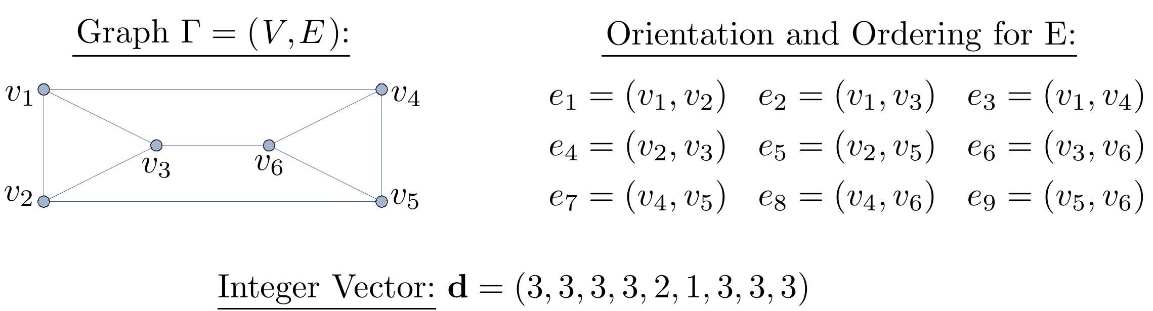
Figure 3: $3$-GKM Skeleton of Example 5.45

The structure matrix is

$$\mathbf{A}=\left(\begin{array}[]{rrrrrrrrr}$2$&$1$&$1$&$-1$&$-1$&$0$&$0$&$0$&$0$\\ $1$&$2$&$1$&$1$&$0$&$-1$&$0$&$0$&$0$\\ $1$&$1$&$2$&$0$&$0$&$0$&$-1$&$-1$&$0$\\ $-1$&$1$&$0$&$2$&$1$&$-1$&$0$&$0$&$0$\\ $-1$&$0$&$0$&$1$&$2$&$0$&$1$&$ 0$&$-1$\\ $0$&$-1$&$0$&$-1$&$0$&$2$&$0$&$1$&$1$\\ $0$&$0$&$-1$&$0$&$1$&$0$&$2$&$1$&$-1$\\ $0$&$0$&$0$&$0$&$-1$&$1$&$-1$&$1$&$2$\\ \end{array}\right).$$

The defect of this $3$-GKM skeleton is $3$ and a fundamental system is given by

$$\quad\,\,\,f_{1}\,\,\,\,f_{2}\,\,\,\,\,f_{3}\,\,\,\,f_{4}\,\,\,f_{5}\,\,\,f_{6}\,\,\,f_{7}\,\,\,f_{8}\,\,\,f_{9}$$

$$\left(\begin{array}[]{rrrrrrrrr}$-1$&$0$&$0$&$1$&$0$&$0$&$-1$&$0$&$1$\\ $1$&$1$&$0$&$0$&$0$&$0$&$1$&$1$&$0$\\ $1$&$2$&$3$&$1$&$3$&$3$&$0$&$0$&$0$\\ \end{array}\right).$$

The Kernel Condition (K1) is satisfied. But the Kernel Condition (K2) is not satisfied, it fails to be true at the edges $e_{3}$, $e_{5}$ and $e_{6}$. Now we use Lemma 5.44 to show that this $3$-GKM skeleton does not support an abstract GKM-graph. First consider the edge $e_{3}=(v_{1},v_{4})$. There exist exactly two connections along $e_{3}$, namely

$$\nabla_{e_{3}}:\,\,\left\{\begin{array}[]{r}(v_{1},v_{2})\mapsto(v_{4},v_{6})\\ (v_{1},v_{3})\mapsto(v_{4},v_{5})\\ (v_{1},v_{4})\mapsto(v_{4},v_{1})\end{array}\right\}\quad\text{and}\quad\nabla^{\prime}_{e_{3}}:\,\,\left\{\begin{array}[]{r}(v_{1},v_{2})\mapsto(v_{4},v_{5})\\ (v_{1},v_{3})\mapsto(v_{4},v_{6})\\ (v_{1},v_{4})\mapsto(v_{4},v_{1})\end{array}\right\}.$$

We have

$$\operatorname{IND}_{v_{1}}=\{1,2,3\}\quad\text{and}\quad\operatorname{IND}_{v_{4}}=\{3,7,8\}$$

and the maps $\operatorname{IND}_{v_{1}}\rightarrow\operatorname{IND}_{v_{4}}$ induced by the two connections along $e_{3}$ are given by

$$\widetilde{\nabla}_{3}:\,\,\left\{\begin{array}[]{r}1\mapsto 8\\ 2\mapsto 7\\ 3\mapsto 3\end{array}\right\}\quad\text{and}\quad\widetilde{\nabla}^{\prime}_{3}:\,\,\left\{\begin{array}[]{r}1\mapsto 7\\ 2\mapsto 8\\ 3\mapsto 3\end{array}\right\}.$$ (5.33)

Note that

$$a_{3,1}\cdot f_{1}+a_{3,\widetilde{\nabla}_{3}(1)}\cdot f_{\widetilde{\nabla}_{3}(1)}=a_{3,1}\cdot f_{1}+a_{3,8}\cdot f_{8}=(-1,0,1)^{\intercal}$$

$$a_{3,2}\cdot f_{2}+a_{3,\widetilde{\nabla}_{3}(2)}\cdot f_{\widetilde{\nabla}_{3}(2)}=a_{3,1}\cdot f_{2}+a_{3,7}\cdot f_{7}=(1,0,2)^{\intercal}$$

$$a_{3,3}\cdot f_{3}+a_{3,\widetilde{\nabla}_{3}(3)}\cdot f_{\widetilde{\nabla}_{3}(3)}=a_{3,3}\cdot f_{1}+a_{3,3}\cdot f_{3}=(0,0,12)^{\intercal}.$$

and since $f_{3}=(0,0,3)^{\intercal}$, the connection $\nabla_{e_{3}}$ does not fail (K2) by a rational number. But since

$$a_{3,1}\cdot f_{1}+a_{3,\widetilde{\nabla}^{\prime}_{3}(1)}\cdot f_{\widetilde{\nabla}^{\prime}_{3}(1)}=a_{3,1}\cdot f_{1}+a_{3,7}\cdot f_{7}=\frac{1}{3}\cdot f_{3}.$$

the connection $\nabla_{e_{3}}^{\prime}$ fails (K2) by a rational number. Hence, there exists only one connection along $e_{3}$ that does not fail (K2) by a rational number, namely $\nabla_{e_{3}}$. Now consider the edge $e_{5}=(v_{2},v_{6})$. As above, we can show that there exists exactly one connection $\nabla_{e_{5}}$ along $e_{5}$ that does not fail (K2) by a rational number. We have

$$\operatorname{IND}_{v_{2}}=\{1,4,5\}\quad\text{and}\quad\operatorname{IND}_{v_{5}}=\{5,7,9\}$$

and the map $\operatorname{IND}_{v_{2}}\rightarrow\operatorname{IND}_{v_{5}}$ induced by the connection $\nabla_{e_{5}}$ is given by

$$\widetilde{\nabla}_{5}:\,\,\left\{\begin{array}[]{r}1\mapsto 9\\ 4\mapsto 7\\ 5\mapsto 5\end{array}\right\}.$$

Now fix the indices

$$1\in\operatorname{IND}_{v_{1}}\setminus\left\{3\right\}\quad\text{and}\quad 5\in\operatorname{IND}_{v_{2}}\setminus\left\{5\right\}$$

and let

$$h_{1}=a_{3,1}f_{1}+a_{3,8}f_{8}=(-1,0,1)^{\intercal}$$

$$h_{2}=a_{5,1}f_{5}+a_{5,9}f_{9}=(0,-1,-1)^{\intercal}.$$

These both vector are non-zero. Moreover, we have $f_{3}=f_{5}$ and the matrix

$$\left(\begin{matrix}|&|&|&|\\ f_{3}&f_{5}&h_{1}&h_{2}\\ |&|&|&|\end{matrix}\right)$$

has rank $3$. Hence, by Lemma 5.44 the $3$-GKM skeleton does not support an abstract GKM graph.

We formulate Lemma 5.44 as a test that gives a necessary condition for a $3$-GKM skeleton with defect $3$ that does not satisfy the Kernel Condition (K2) to support an abstract $(3,2)$-GKM graph. We call this test the Projection Test. So let $(\Gamma,\sigma,\operatorname{Ord}(E^{\sigma}),\mathbf{d})$ be such a $3$-GKM skeleton and let $f_{1},\dots,f_{\frac{1}{2}\left|E\right|}$ be a fundamental system.

The Projection Test

• First let $\operatorname{ListKern}=\left\{\right\}$ be an empty list.

• Start with $j=1$ and do the following as long as $j\leq\frac{1}{2}\left|E\right|$. Check if the Kernel Condition (K2) at $e_{j}$ is satisfied.

  • If (K2) is satisfied at $e_{j}$, set $j\rightarrow j+1$.

  • If (K2) is not satisfied at $e_{j}$, then let $k_{1}\in\operatorname{IND}_{i(e_{j})}\setminus\{j\}$ and $k_{2},k_{3}\in\operatorname{IND}_{t(e_{j})}\setminus\{j\}$.
    Check if the conditions

    $$(*)\quad\quad\,\,a_{j,k_{1}}\cdot f_{k_{1}}+a_{j,k_{2}}\cdot f_{k_{2}}=\nu_{1}\cdot f_{j}\,\,\,\,\text{for some}\,\,\nu_{1}\in\mathbb{Q}\setminus\mathbb{Z}\quad\text{and}$$

    $$(**)\quad\quad a_{j,k_{1}}\cdot f_{k_{1}}+a_{j,k_{3}}\cdot f_{k_{3}}=\nu_{2}\cdot f_{j}\,\,\,\,\text{for some}\,\,\nu_{2}\in\mathbb{Q}\setminus\mathbb{Z}$$

    are satisfied.

    • If $(*)$ and $(**)$ are true, set $j\rightarrow\frac{1}{2}\left|E\right|+2$.

    • If $(*)$ and $(**)$ are false, set $j\rightarrow j+1$.

    • If $(*)$ is true and $(**)$ is false, then add the $(3\times 2)$ matrix

      $$\left(\begin{matrix}|&|\\ f_{j}&a_{j,k_{1}}\cdot f_{k_{1}}+a_{j,k_{3}}\cdot f_{k_{3}}\\ |&|\end{matrix}\right)$$

      to the list $\operatorname{ListKern}$ and set $j\rightarrow j+1$.

    • If $(*)$ is false and $(**)$ is true, then add the $(3\times 2)$ matrix

      $$\left(\begin{matrix}|&|\\ f_{j}&a_{j,k_{1}}\cdot f_{k_{1}}+a_{j,k_{2}}\cdot f_{k_{2}}\\ |&|\end{matrix}\right)$$

      to the list $\operatorname{ListKern}$ and set $j\rightarrow j+1$.

• • If $j=\frac{1}{2}\left|E\right|+2$, then

    Output: The Projection Test is not satisfied.

  • If $j=\frac{1}{2}\left|E\right|+1$ and if the list $\operatorname{ListKern}$ is empty or contains only one element, then

    Output: The Projection Test makes no statement.

  • If $j=\frac{1}{2}\left|E\right|+1$ and if the list $\operatorname{ListKern}$ contains at least two elements, then check for any two elements

    $$\left(\begin{matrix}|&|\\ \alpha_{1}&\beta_{1}\\ |&|\end{matrix}\right)\quad\text{and}\quad\left(\begin{matrix}|&|\\ \alpha_{2}&\beta_{2}\\ |&|\end{matrix}\right)$$

    of $\operatorname{ListKern}$ if one the vector pairs $(\alpha_{1},\alpha_{2})$, $(\alpha_{1},\beta_{2})$, $(\beta_{1},\alpha_{2})$, if $\beta_{1}$ and $\beta_{2}$ are both non-zero and $(\beta_{1},\beta_{2})$ is linearly dependent and if the matrix

    $$\left(\begin{matrix}|&|&|&|\\ \alpha_{1}&\alpha_{1}&\beta_{1}&\beta_{2}\\ |&|&|&|\end{matrix}\right)$$

    has rank $3$. If this holds, then

    Output: The GKM skeleton does not support an abstract GKM graph.

    otherwise

    Output: The Projection Test makes no statement.

5.3 Positive Hamiltonian Abstract $(3,d)$-GKM Graphs

In this subsection we formulate necessary conditions for an abstract $(3,d)$-GKM graph $(\Gamma,\operatorname{w})$ to be realizable by a Hamiltonian GKM space $(M,\omega,T,\phi)$ of dimension six, i.e., the isomorphism class of the abstract GKM graph $(\Gamma,\operatorname{w})$ is in the image of the isomorphism class of the GKM graph of $(M,\omega,T,\phi)$ under the map $\mathcal{L}_{3,d}$ of (5.7).

Definition 5.46.

Let $(\Gamma,\operatorname{w})$ be an abstract $(3,d)$-GKM graph. We say that $(\Gamma,\operatorname{w})$ satisfies the $\mathbf{24}$-Rule if for any orientation $\sigma$ of the edge set, we have

$$\sum_{e\in E^{\sigma}}\mathcal{C}_{1}(e)=24.$$

Here $\mathcal{C}_{1}:E\rightarrow\mathbb{Z}$ is the first Chern class map of $(\Gamma,\operatorname{w})$.

Definition 5.47.

An abstract $(n,d)$-GKM graph $(\Gamma,\operatorname{w})$ is called positive if $\mathcal{C}_{1}(e)>0$ for all $e\in E$.

We deduce necessary conditions for an abstract $(3,d)$-GKM to be realizable by a (positive) Hamiltonian GKM space.

Corollary 5.48.

Let $(\Gamma,\operatorname{w})$ be an abstract $(3,d)$-GKM graph.

• If $(\Gamma,\operatorname{w})$ is Hamiltonian, i.e., it is realizable by a Hamiltonian GKM space of dimension six, then $(\Gamma,\operatorname{w})$ satisfies the $24$-Rule.

• If $(\Gamma,\operatorname{w})$ is realizable by a positive Hamiltonian GKM space of dimension six, then $(\Gamma,\operatorname{w})$ is positive. In particular, the number of vertices of $\Gamma$ is at most $16$.

Proof.

• This follows directly form Corollary 4.12 $(ii)$ and Remark 5.11.

• That $(\Gamma,\operatorname{w})$ is positive follows from Remark 5.11. That the number of vertices is at most $16$ follows from Corollary 4.12 $(iii)$.

∎

We note that Definitions 5.46 and 5.47 extend naturally to GKM skeletons.

Definition 5.49.

Let $(\Gamma,\sigma,\operatorname{Ord}(E^{\sigma}),\mathbf{d})$ be an $n$-GKM skeleton. The skeleton is called positive if $d_{j}>0$ for all $j=1,\dots,\frac{1}{2}\left|E\right|$, where $d_{j}$ is the $j$-th entry of the integer vector $\mathbf{d}$. If $n=3$, then $(\Gamma,\sigma,\operatorname{Ord}(E^{\sigma}),\mathbf{d})$ satisfies the $24$-Rule if

$$d_{1}+...+d_{\frac{1}{2}\left|E\right|}=24.$$

The following is a direct consequence of Corollary 5.48.

Corollary 5.50.

Let $(\Gamma,\sigma,\operatorname{Ord}(E^{\sigma}),\mathbf{d})$ be a $3$-GKM skeleton that supports a positive Hamiltonian abstract $(3,d)$-GKM graph. Then the skeleton is positive and satisfies the $24$-Rule. In particular, the number of the vertices of the graph $\Gamma$ is at most $16$.

By Corollary 5.48, necessary conditions for an abstract $(3,d)$-GKM graph to be realizable by a positive Hamiltonian GKM space of dimension six are the 24-Rule and the positive condition. These conditions are not sufficient, as we show in Example 5.57. To show this, we use the existence of the special Kirwan class. In the following, we extend the definition of a generic vector and an ascending path to abstract GKM graphs. We use these terms to formulate a necessary condition for a positive abstract $(3,d)$-GKM graph to be Hamiltonian: the Kirwan Class Test.

Definition 5.51.

Let $(\Gamma,\operatorname{w})$ be an abstract $(n,d)$-GKM graph. A vector $\xi\in\mathbb{R}^{d}$ is generic if for any edge $e\in E$

$$\left\langle\operatorname{w}(e),\xi\right\rangle_{\mathbb{R}^{d}}\neq 0,$$

where $\left\langle\cdot,\cdot\right\rangle_{\mathbb{R}^{d}}$ is the standard scalar product on $\mathbb{R}^{d}$.
For a vertex $v\in V$, its index $\lambda(v)$ with respect to $\xi$ is equal to the number of edges that satisfy

$$e\in E_{v}^{i}\quad\text{and}\quad\left\langle\operatorname{w}(e),\xi\right\rangle_{\mathbb{R}^{d}}<0.$$ (5.34)

For a vertex $v\in V$ with $\lambda(v)=1$, its negative Euler class with respect to $\xi$ is

$$\tau_{v}^{-}:=\operatorname{w}(e),$$

where $e$ is the unique edge that satisfies (5.34).

An ascending path from a vertex $v$ to another vertex $w$ is a $(k+1)$-tuple $(v_{0},...,v_{k})$ of vertices in $V$ such that $v_{0}=v$, $v_{k}=w$ and

$$(v_{i-1},v_{i})\in E\,\,\text{and}\,\,\left\langle\operatorname{w}(v_{i}),\xi\right\rangle_{\mathbb{R}^{d}}>0.$$

Moreover, for each vertex $v\in V$, the stable set of $v$, denoted by $\Xi_{v}$, is the set of vertices $w\in V$ such that there exists an ascending path from $v$ to $w$, including $v$ itself.

Lemma 5.52.

Let $(\Gamma,\operatorname{w})$ be a positive and Hamiltonian abstract $(3,d)$-GKM graph. Let $\xi\in\mathbb{R}^{d}$ be a generic vector and let $v\in V$ be a vertex with $\lambda(v)=1$. Then there exists a map $\gamma_{v}:V\rightarrow\mathbb{Z}^{d}$ such that

• $\gamma_{v}(w)=0$ if $\lambda(w)=0,1$ and $w\notin\Xi_{v}$.

• $\gamma_{v}(w)=\tau_{v}^{-}$ if $\lambda(w)=1$ and $w\in\Xi_{v}$.

• For each edge $e=(v_{1},v_{2})\in E$ the difference $\gamma_{v}(v_{1})-\gamma_{v}(v_{2})$ is an integer multiple of $\operatorname{w}(e)$.

Proof.

Since $(\Gamma,\operatorname{w})$ is Hamiltonian, there exits a Hamiltonian GKM space $(M,\omega,T,\phi)$ of dimension $6$ with $\operatorname{dim}(T)=d$ and a linear isomorphism $\chi:\ell_{T}^{*}\rightarrow\mathbb{Z}^{d}$ such that $\Gamma_{GKM}=\Gamma$ and $\operatorname{w}=\chi\circ\eta$, where $(\Gamma_{GKM},\eta)$ is the GKM graph of $(M,\omega,T,\phi)$. Let $\bar{\xi}\in\mathfrak{t}$ the unique vector that satisfies

$$\left\langle\eta(e),\bar{\xi}\right\rangle=\left\langle\operatorname{w}(e),\xi\right\rangle_{\mathbb{R}^{d}}$$

for all $e\in E=E_{GKM}$, where $\left\langle\cdot,\cdot\right\rangle$ is the natural pairing between $\mathfrak{t}$ and $\mathfrak{t}^{\prime}$. Note that the vector $\bar{\xi}$ is generic for the $T$-action, as defined in Subsection 2.3.1, and the index of $v$ as a vertex is equal to the index of $v$ as a fixed point with respect to $\phi^{\bar{\xi}}$. Moreover, a path in $\Gamma$ is ascending with respect to $\bar{\xi}$ as in Definition 4.15 if and only if it is ascending with respect to $\xi$. Note that since $(\Gamma,\sigma,\operatorname{Ord}(E^{\sigma}),\mathbf{d})$ is positive, we have that $(\Gamma_{GKM},\eta)$ is positive. So by Lemma 4.14, $(\Gamma_{GKM},\eta)$ is weak indexing increasing with respect to $\bar{\xi}$. Hence, by Proposition 4.17, there exists a class

$$\widehat{\gamma_{v}}\in H_{T}^{2}(M;\mathbb{Z})\subset\operatorname{Maps}(V,\ell_{T}^{*})$$

such that

• $\widehat{\gamma_{v}}(w)=0$ if $\lambda(w)=0,1$ and $w\notin\Xi_{v}$ and

• $\widehat{\gamma_{v}}(w)=\Lambda_{v}^{-}$ if $\lambda(w)=1$ and $w\in\Xi_{v}$,

where $\Lambda_{v}^{-}\in\ell_{T}^{*}$ is the equivariant Euler class of the negative tangent bundle at $v$ with respect to $\phi^{\bar{\xi}}$. Note that since $\lambda(v)=1$, the class $\Lambda_{v}^{-}$ equals the unique weight $\alpha_{v}$ such that $\left\langle\alpha_{v},\bar{\xi}\right\rangle<0$, which equals $\eta(e)$ for the unique edge such that $\left\langle\eta(e),\bar{\xi}\right\rangle<0$. So $\Lambda_{v}^{-}$ is mapped under $\chi$ to $\tau_{v}^{-}=\operatorname{w}(e)$. Therefore the map

$$\gamma_{v}=\chi\circ\widehat{\gamma_{v}}:V\rightarrow\mathbb{Z}^{d}$$

satisfies the properties (i) and (ii). Moreover, since $\widehat{\gamma_{v}}\in H_{T}^{2}(M;\mathbb{Z})$, we have that for each edge $e=(v_{1},v_{2})\in E$, the difference $\widehat{\gamma_{v}}(v_{1})-\widehat{\gamma_{v}}(v_{2})$ is an integer multiple of $\eta(e)$. So $\gamma_{v}$ satisfies also (iii). ∎

Definition 5.53.

Let $(\Gamma,\operatorname{w})$ be an abstract $(n,d)$-GKM graph. The weight sum map for this abstract GKM graph is the map $\varphi:V\rightarrow\mathbb{Z}^{d}$ given by

$$\varphi(v)=-\sum_{e\in E_{v}^{i}}\operatorname{w}(e).$$

Moreover, for a given vector $\xi\in\mathbb{R}^{\delta}$ the $\xi$-component, $\varphi^{\xi}:V\rightarrow\mathbb{R}$, of $\varphi$ is given by

$$\varphi^{\xi}(v)=\left\langle\varphi(v),\xi\right\rangle_{\mathbb{R}^{d}}.$$

Lemma 5.54.

Let $(\Gamma,\operatorname{w})$ be an abstract $(n,d)$-GKM graph that is positive. Let $\xi\in\mathbb{R}^{d}$ be a generic vector. For any edge $e=(v,w)$ with $\left\langle\operatorname{w}(e),\xi\right\rangle_{\mathbb{R}^{d}}<0$ we have

$$\varphi^{\xi}(v)>\varphi^{\xi}(w).$$

Proof.

Let $e=(v,w)$ be an edge with $\left\langle\operatorname{w}(e),\xi\right\rangle_{d}<0$ . By the construction of the weight sum map we have

$$\varphi(v)-\varphi(w)=-\mathcal{C}_{1}(e)\cdot{\operatorname{w}}(e),$$

Since $(\Gamma,\operatorname{w})$ is positive, we have in particular $\mathcal{C}_{1}(e)>0$. So we have that

$$\varphi^{\xi}(v)-\varphi^{\xi}(w)=-\mathcal{C}_{1}(e)\cdot\left\langle{\operatorname{w}}(e),\xi\right\rangle_{\mathbb{R}^{d}}>0.$$

∎

Remark 5.55.

Let $(\Gamma,\operatorname{w})$ be an abstract $(3,d)$-GKM graph that is positive and Hamiltonian. Let $\xi\in\mathbb{R}^{d}$ be a generic vector. Given $v\in V$ with $\lambda(v)=1$, let $\gamma_{v}:V\rightarrow\mathbb{Z}^{d}$ be a map as in Lemma 5.52. We know $\gamma_{v}(w)$ for vertices with $\lambda(w)\leq 1$. For vertices with $\lambda(w)\geq 2$ it can be computed. Let $\varphi^{\xi}:V\rightarrow\mathbb{R}$ be the $\xi$-component of the weight sum map. Let $w_{1},\dots,w_{k}$ be the vertices with index greater than one, ordered so that

$$\varphi^{\xi}(w_{1})\leq\varphi^{\xi}(w_{2})\leq\dots\leq\varphi^{\xi}(w_{k}).$$

Suppose we have already computed $\gamma_{v}(w_{i})$ for $i=1,...,j$, where $j<k$. Since $\lambda(w_{j+1})\geq 2$, there exist two different vertices $r_{1},r_{2}\in V$ with $e:=(w_{j+1},r_{1}),e^{\prime}:=(w_{j+1},r_{2})\in E$ and

$$\left\langle{\operatorname{w}}(e),\xi\right\rangle_{\mathbb{R}^{d}}<0\quad\text{and}\quad\left\langle{\operatorname{w}}(e^{\prime}),\xi\right\rangle_{\mathbb{R}^{d}}<0.$$

By Lemma 5.54 we have $\varphi^{\xi}(r_{1})<\varphi^{\xi}(q_{j+1})$. If $\lambda(r_{1})\geq 2$, we have $r_{1}=w_{i}$ for some $i=1,...,j$, so we have already computed $\gamma_{v}(r_{1})$. If $\lambda(r_{1})\leq 1$, we also know $\gamma_{v}(r_{1})$. For the same reason we know $\gamma_{v}(r_{2})$. By property (iii) of $\gamma_{v}$, there exist integers $A_{1}$ and $A_{2}$ such that

$$\gamma_{v}(w_{j+1})-\gamma_{v}(r_{1})=A_{1}\cdot{\operatorname{w}}(w_{j+1},r_{1})\quad\text{and}\quad\gamma_{v}(w_{j+1})-\gamma_{v}(r_{2})=A_{2}\cdot(w_{j+1},r_{2}).$$

So we have

$$\gamma_{v}(r_{1})-\gamma_{v}(r_{2})=-A_{1}\cdot{\operatorname{w}}(w_{j+1},r_{1})+A_{2}\cdot{\operatorname{w}}(w_{j+1},r_{2}).$$

Since we know $\gamma_{v}(r_{1})$ and $\gamma_{v}(r_{2})$ and since ${\operatorname{w}}(w_{j+1},r_{1})$ and ${\operatorname{w}}(w_{j+1},r_{2})$ are linearly independent, we can compute $A_{1}$ and $A_{2}$. So we have

$$\gamma_{v}(w_{j+1}) =\gamma_{v}(r_{1})+A_{1}\cdot{\operatorname{w}}(w_{j+1},r_{1})\,\,\text{resp.}$$

$$\gamma_{v}(w_{j+1}) =\gamma_{v}(r_{2})+A_{2}\cdot{\operatorname{w}}(w_{j+1},r_{2}).$$

Remark 5.56.

Let $(\Gamma,\operatorname{w})$ be an abstract $(3,d)$-GKM graph that is positive. Let $\xi\in\mathbb{R}^{d}$ be a generic vector. If for each vertex $v\in V$ with $\lambda(v)=1$, there exists a class $\gamma_{v}:V\rightarrow\mathbb{Z}^{d}$ as in Lemma 5.52, then we say that $(\Gamma,\operatorname{w})$ satisfies the Kirwan Class Test with respect to $\xi$. Note that if $(\Gamma,\operatorname{w})$ is Hamiltonian then the Kirwan Class Test is satisfied. By Remark 5.55, it is easy to check whether the Kirwan Class Test is satisfied.

Example 5.57.

Consider the abstract $(3,2)$-GKM graph $(\Gamma,\operatorname{w})$ with six vertices that we visualize in Figure 4. The big dots mark the vertices resp. the images of the vertices under the weight sum map $\varphi$ in $\mathbb{Z}^{2}$. The small dots mark the other points of $\mathbb{Z}^{2}$ that lie in the convex hull of the images of the vertices under $\varphi$. For two different vertices $v_{i}$ and $v_{j}$, the pair $(v_{i},v_{j})$ is an edge of the graph $\Gamma$ if and only if there exists a line segment from the dot $v_{i}$ to the dot $v_{j}$. If $(v_{i},v_{j})$ is an edge and the line segment is blue, then $\operatorname{w}(v_{i},v_{j})$ is the primitive vector that points in the direction of the oriented line segment from $v_{i}$ to $v_{j}$. If the line segment is red, then $\operatorname{w}(v_{i},v_{j})$ is the double of this primitive vector. For example

$$\operatorname{w}(v_{1},v_{2})=(-1,2)^{\intercal}\quad\text{and}\quad\operatorname{w}(v_{1},v_{6})=(2,0)^{\intercal}.$$

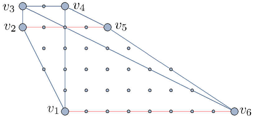
Figure 4: The abstract GKM graph of Example 5.57

Moreover, let $(v_{i},v_{j})\in E$ be an edge and let $l$ be the number of points in $\mathbb{Z}^{2}$ that lie on the line segment between the dots $v_{i}$ and $v_{j}$, then

$$\mathcal{C}_{1}(v_{i},v_{j})=\begin{cases}l-1\quad\,\,\,\,\,\,\,\,\text{if the line segment is blue,}\\ \frac{1}{2}(l-1)\quad\text{if the line segment is red.}\end{cases}$$

For example,

$$\mathcal{C}_{1}(v_{1},v_{2})=2\quad\text{and}\quad\mathcal{C}_{1}(v_{1},v_{6})=4.$$

So this abstract GKM graph is positive and satisfies the $24$-Rule.

We show by contradiction that this abstract GKM graph is not Hamiltonian.
The vector $\xi=(1,1)^{\intercal}\in\mathbb{R}^{2}$ is generic for this abstract GKM graph. The indices, the stable sets of vertices, and the weight sum map and its $\xi$-component are given in Table 1.

	Index $\lambda$	$\varphi$	$\varphi^{\xi}$	$\Xi_{v_{i}}$
$v_{1}$	0	(-1,-3$)^{\intercal}$	-4	$\{v_{1},v_{2},v_{3},v_{4},v_{5},v_{6}\}$
$v_{2}$	1	(-3,1$)^{\intercal}$	-2	$\{v_{2},v_{3},v_{4},v_{5},v_{6}\}$
$v_{3}$	1	(-3,2$)^{\intercal}$	-1	$\{v_{3},v_{4},v_{5},v_{6}\}$
$v_{4}$	2	(-1,2$)^{\intercal}$	1	$\{v_{4},v_{5},v_{6}\}$
$v_{5}$	2	(1,1$)^{\intercal}$	2	$\{v_{5},v_{6}\}$
$v_{6}$	3	(7,-3$)^{\intercal}$	4	$\{v_{6}\}$

Table 1: Values of $\varphi$ resp. $\varphi^{\xi}$ and $\Xi_{v_{i}}$.

The vertex $v_{2}$ has index one and the unique edge $e\in E$ with $e\in E_{v_{4}}^{i}$ and $\left\langle\operatorname{w}(e),\xi\right\rangle_{\mathbb{R}^{2}}<0$ is $(v_{2},v_{1})$. Hence, the negative Euler class of $v_{2}$ with respect to $\xi$ is

$$\tau_{v_{2}}^{-}=\operatorname{w}(v_{2},v_{1})=(1,-2)^{\intercal}.$$

Now assume by negation that $(\Gamma,\operatorname{w})$ is Hamiltonian. By Lemma 5.52 there exists a map $\gamma_{v_{2}}:V\rightarrow\mathbb{Z}^{2}$ such that

$$\gamma_{v_{2}}(v_{1})=(0,0)^{\intercal},\quad\gamma_{v_{2}}(v_{2})=\gamma_{v_{2}}(v_{3})=(1,-2)^{\intercal}$$

and for any edge $(v_{i},v_{j})$ the difference $\gamma_{v_{2}}(v_{i})-\gamma_{v_{2}}(v_{j})$ is an integer multiple of $\operatorname{w}(v_{i},v_{j})$. The vertices with index greater than one are $v_{4}$,$v_{5}$ and $v_{6}$ and we have

$$\varphi^{\xi}(v_{4})<\varphi^{\xi}(v_{5})<\varphi^{\xi}(v_{6}).$$

As in Remark 5.55, we can compute $\gamma_{v_{2}}(v_{4})$, after that $\gamma_{v_{2}}(v_{5})$, and then $\gamma_{v_{2}}(v_{6})$.

We have $(v_{4},v_{1}),(v_{4},v_{3})\in E$. So there exist integers $A_{1}$ and $A_{2}$ such that

$$\gamma_{v_{2}}(v_{4})-\gamma_{v_{2}}(v_{1})=A_{1}\cdot{\operatorname{w}}(v_{4},v_{1})\quad\text{and}\quad\gamma_{v_{2}}(v_{4})-\gamma_{v_{2}}(v_{3})=A_{2}\cdot{\operatorname{w}}(v_{4},v_{3}).$$

This leads to

$$(-1,2)^{\intercal}=\gamma_{v_{2}}(v_{1})-\gamma_{v_{2}}(v_{3})=-A_{1}\cdot(0,-1)^{\intercal}+A_{2}\cdot(-1,0)^{\intercal}.$$

Hence, $A_{1}=2$ , $A_{2}=1$ and $\gamma_{v_{4}}(v_{2})=(0,-2)^{\intercal}$.

Moreover, we have $(v_{5},v_{2}),(v_{5},v_{4})\in E$. So there exist integers $B_{1}$ and $B_{2}$ such that

$$\gamma_{v_{2}}(v_{5})-\gamma_{v_{2}}(v_{2})=B_{1}\cdot{\operatorname{w}}(v_{5},v_{2})\quad\text{and}\quad\gamma_{v_{2}}(v_{5})-\gamma_{v_{2}}(v_{4})=B_{2}\cdot{\operatorname{w}}(v_{5},v_{4}).$$

This leads to

$$(1,0)^{\intercal}=\gamma_{v_{2}}(v_{2})-\gamma_{v_{2}}(v_{4})=-B_{1}\cdot(-2,0)^{\intercal}+B_{2}\cdot(-2,1)^{\intercal}.$$

But this implies $B_{1}=\frac{1}{2}\notin\mathbb{Z}$, which is a contradiction.

6 About the Computer Programs

In order to list all GKM graphs that are coming from positive Hamiltonian GKM spaces of dimension six, we need to consider all positive $3$-GKM skeletons that satisfy the $24$-Rule up to isomorphism. The underlying graph of such a skeleton is connected, simple and $3$-valent, i.e., a cubic graph, with at most $16$ vertices; see Corollary 5.50. The data base [4] provides the complete list of cubic graphs with at most $16$ vertices. Here, for $X=4,6,...,16$, we refer to the list that contains all (isomorphism classes of) cubic graphs with exactly $X$ vertices as $CubicGraphsX$. We refer to the graph that is the $j$-th element of the list $CubicGraphsX$ as CX.j. Let $\Gamma$ be a graph in the list $CubicGraphsX$. Note that the number of edges is $3\cdot X$ and that if there exists a map $\operatorname{w}:E\rightarrow\mathbb{Z}^{2}\setminus\{0\}$ such that $(\Gamma,\operatorname{w})$ is an abstract positive $(3,d)$-GKM graph that is Hamiltonian, then for any orientation $\sigma$ of the edge set and any ordering $\operatorname{Ord}(E^{\sigma})$ there exists an integer vector $\mathbf{d}\in\mathbb{Z}_{>0}^{\frac{3}{2}X}$ with

$$d_{1}+...+d_{\frac{3}{2}X}=24$$

such that the GKM skeleton $(\Gamma,\sigma,\operatorname{Ord}(E^{\sigma}),\mathbf{d})$ has defect greater or equal to $d$ and satisfies the Kernel Condition (K1), see Proposition 5.23 and Corollary 5.31; note that since $n=3$, we have $d\geq 2$, see Remark 5.4. The following computer program computes the list $GraphsToBeConsideredX$ that contains all cubic graphs with $X\leq 16$ vertices that satisfy these conditions.

Program: Compute the List $GraphsToBeConsideredX$

• Compute the list $Permutations$ that contains all integer vectors $\mathbf{d}\in\mathbb{Z}_{>0}^{\frac{3}{2}X}$ that satisfy

  $$d_{1}+...+d_{\frac{3}{2}X}=24.$$

• Let $GraphsToBeConsideredX$=$\left\{\right\}$ be the empty list.

• Do the following for each graph $\Gamma$ in the list $CubicGraphsX$. Fix an orientation $\sigma$ of the edge set and an ordering $\operatorname{Ord}(E^{\sigma})$.
  Start with $j=1$ and do the following as long as $j\leq\operatorname{Length}[Permutations]$.
  Let $\mathbf{d}$ be the $j$-th element of the list $Permutations$.

  • If the GKM skeleton $(\Gamma,\sigma,\operatorname{Ord}(E^{\sigma}),\mathbf{d})$ has a defect greater than one and satisfies the Kernel Condition (K1), then add $\Gamma$ to the list $GraphsToBeConsideredX$ and set

    $$j\rightarrow\operatorname{Length}[Permutations]+1.$$

  • If not, then set $j\rightarrow j+1.$

The result of this program is given in Table 2. Note that in total there are only $14$ cubic graphs that belong to the list $GraphsToBeConsideredX$ for some $X=4,6,\dots,16$. If a $3$-GKM skeleton supports a positive and Hamiltonian abstract GKM graph, then the underlying graph is isomorphic to one of these $14$ graphs.

X	Number of Cubic Graphs with X vertices	$GraphsToBeConsideredX$
4	1	C4.1
6	2	C6.1, C6.2
8	5	C8.2, C8.4, C8.5
10	19	C10.11, C10.15, C10.16, C10.17
12	85	C12.68, C12.69, C12.71, C12.74
14	509	empty list
16	4060	empty list
	total: 4681	total: 14

Table 2: Lists of graphs that need to be considered.

With the following computer program, we analyze the 14 cubic graphs. Recall that if a $3$-GKM skeleton supports an abstract $(3,d)$-GKM graph then for the defect $\delta$ of the skeleton we have $\delta\geq d\geq 2$. If $\delta=d$ then the Kernel Condition (K2) is a necessary condition for a $3$-GKM skeleton to support an abstract $(3,d)$-GKM graph; see Corollary 5.35. If the Kernel Conditions (K1) and (K2) both hold, the $3$-GKM skeleton supports a unique -up to isomorphism and projection- abstract $(3,\delta)$-GKM graph; see Proposition 5.38. In case $\delta=2$ and both Conditions (K1) and (K2) hold, we use the Kirwan Class Test to detect if the abstract GKM graph fails to be Hamiltonian; see Lemma 5.52 and Remark 5.56. If $\delta=3$ and the Kernel Condition (K2) does not hold, we use the Projection Test (see Subsection 5.2.4) to detect if the $3$-GKM skeleton fails to support an abstract GKM graph.

Program: Analyze the Cubic Graphs

• Fix an orientation $\sigma$ of the edge set and an ordering $\operatorname{Ord}(E^{\sigma})$.

• Compute the list $Permutations1$ that contains all integer vectors $\mathbf{d}\in\mathbb{Z}_{>0}^{\frac{3}{2}X}$ that satisfy

  $$d_{1}+...+d_{\frac{3}{2}X}=24.$$

• Let $Permutations2$ be the list that contains only the first element of $Permutations1$.
  Start with $j=2$ and do the following as long as $j\leq\operatorname{Length}[Permutations1]$.
  Let $\mathbf{d}$ be the $j$-th element of the list $Permutations1$. If there exists no $j^{\prime}<j$ such that $(\Gamma,\sigma,\operatorname{Ord}(E^{\sigma}),\mathbf{d})$ and $(\Gamma,\sigma,\operatorname{Ord}(E^{\sigma})\mathbf{d^{\prime}})$ are isomorphic GKM skeletons, where $\mathbf{d^{\prime}}$ is the $j^{\prime}$-th element of the list $Permutations1$, then add $\mathbf{d}$ to the list $Permutations2$. Set $j\rightarrow j+1.$

• Start with $j=1$ and do the following as long as $j\leq\operatorname{Length}[Permutations2]$.
  Let $\mathbf{d}$ be the $j$-th element of the list $Permutations2$.

  • If the GKM skeleton $(\Gamma,\sigma,\operatorname{Ord}(E^{\sigma}),\mathbf{d})$ has a defect of two and satisfies the Kernel Conditions (K1) and (K2), apply the Kirwan class test to the GKM skeleton. If the Kirwan Class test is satisfied, then compute a map $\operatorname{w}:E\rightarrow\mathbb{Z}^{2}$ such that $(\Gamma,\operatorname{w})$ is an abstract $(3,2)$-GKM skeleton supported by $(\Gamma,\sigma,\operatorname{Ord}(E^{\sigma}),\mathbf{d})$.

    Output: Give $(\Gamma,\operatorname{w})$.

  • If the GKM skeleton $(\Gamma,\sigma,\operatorname{Ord}(E^{\sigma}),\mathbf{d})$ has a defect of three and satisfies the Kernel Conditions (K1) and (K2), then compute a map $\operatorname{w}:E\rightarrow\mathbb{Z}^{3}$ such that $(\Gamma,\operatorname{w})$ is an abstract $(3,3)$-GKM skeleton supported by $(\Gamma,\sigma,\operatorname{Ord}(E^{\sigma}),\mathbf{d})$.

    Output: Give $(\Gamma,\operatorname{w})$.

  • If the GKM skeleton $(\Gamma,\sigma,\operatorname{Ord}(E^{\sigma}),\mathbf{d})$ has a defect of three and satisfies the Kernel Condition (K1), but not (K2), the apply the Projection Test. If the projection makes no statement, then give the following output.

    Output: The permutation $\mathbf{d}$ need to be considered.

  • If the GKM skeleton $(\Gamma,\sigma,\operatorname{Ord}(E^{\sigma}),\mathbf{d})$ has a defect greater than four and satisfies the Kernel Condition (K1), then give the following output.

    Output: The permutation $\mathbf{d}$ need to be considered.

Apply this program to the $14$ cubic graphs that belong to some list $GraphsToBeConsideredX$. We have the following result.

Proposition 6.1.

Let $(\Gamma,\sigma,\operatorname{Ord}(E^{\sigma}),\mathbf{d})$ be a $3$-GKM skeleton that is positive and that satisfies the $24$-Rule. If $(\Gamma,\sigma,\operatorname{Ord}(E^{\sigma}),\mathbf{d})$ supports an abstract GKM graph $(\Gamma,\operatorname{w})$, then its defect $\delta$ is equal to $2$ or $3$. Moreover, the followings hold.

• If $\delta=2$ and if $(\Gamma,\operatorname{w})$ satisfies the Kirwan class test, then $(\Gamma,\operatorname{w})$ is isomorphic to one of the seven abstract $(3,2)$-GKM graphs that are listed in Appendix A.

• If $\delta=3$, then $(\Gamma,\operatorname{w})$ is a $(3,3)$-abstract GKM graph that comes from a smooth and reflexive polytope or it is the projection of such a $(3,3)$-abstract GKM graph.

6.1 Proof of Theorem 1.8

Recall that if $X$ is a smooth Fano variety endowed with a holomorphic action of an algebraic torus $T_{\mathbb{C}}$, then polarisation of $X$ by its anticanonical line bundle induces a symplectic form $\omega_{X}$ on $X$ such that the induced $T$-action on $X$ is Hamiltonian with respect to $\omega_{X}$ and the induced almost complex structure $J$ is compatible with $\omega_{X}$. Here, $T_{\mathbb{C}}$ is the complexification of $T$.

Proof of Theorem 1.8.

Let $(M,\omega,T,\phi)$ be a positive six-dimensional Hamiltonian GKM space of complexity one and let $(\Gamma_{GKM},\eta)$ be its GKM graph. By Proposition 6.1, $(\Gamma_{GKM},\eta)$ is either isomorphic to one of the seven GKM graphs that are listed in Appendix A or it is the projection of a GKM graph that comes from a smooth and reflexive polytope of dimension three.
The seven GKM graphs in Appendix A are isomorphic to GKM graphs that are coming from holomorphic GKM actions on smooth Fano varieties, as specified in the appendix.
If $(\Gamma_{GKM},\eta)$ is the projection of a GKM graph that comes from a smooth and reflexive polytope $\Delta$ of dimension three, then by Delzant’s classification, Theorem 2.13, there exists a compact symplectic toric manifold $(\widetilde{M},\widetilde{\omega},T\times S^{1},\widetilde{\phi})$ of dimension six such that $\widetilde{\phi}(\widetilde{M})=\Delta$ and an integrable almost complex structure $J$ on $\widetilde{M}$ that is $(T\times S^{1})$-invariant and compatible with $\widetilde{\omega}$. By Proposition 2.16, since the moment map polytope is reflexive, $(\widetilde{M},\widetilde{\omega})$ is positive monotone. Hence, due to the Kodaira Embedding Theorem (see [32, Sect. 14.4]), $\widetilde{M}$ with the complex atlas induced by $J$ is a smooth Fano threefold. By Lemma 5.9, there exists a two-dimensional subtorus $H$ of $T\times S^{1}$ such that the $H$-action is Hamiltonian and GKM and, moreover, $(\Gamma_{GKM},\eta)$ is isomorphic to the GKM graph of the $H$-action on $\widetilde{M}$. ∎

Appendix A Positive Hamiltonian GKM Graphs in Dimension Six

In this appendix we list all positive Hamiltonian GKM graphs in dimension six that are not projections of GKM graphs that are coming from a smooth and reflexive polytope. Up to isomorphism, there exist exactly seven such graphs. We visualize these graphs as in Example 5.57. Namely, the big dots mark the vertices. For two different vertices $v_{i}$ and $v_{j}$, the pair $(v_{i},v_{j})$ is an edge of the graph $\Gamma$ if and only if there exists a line segment connecting the big dots that correspond to dots $v_{i}$ and $v_{j}$. If $(v_{i},v_{j})$ is an edge and the line segment is blue, then $\operatorname{w}(v_{i},v_{j})$ is the primitive vector that points in the direction of the oriented line segment from $v_{i}$ to $v_{j}$. If the line segment is red, then $\operatorname{w}(v_{i},v_{j})$ is the double of this primitive vector. All of these GKM graphs are coming from a holomorphic GKM on smooth Fano varieties. Namely, Süss classified complexity one actions of algebraic tori on smooth Fano threefold [38]. Recall that such an action induces a holomorphic and Hamiltonian action of a compact torus $T=(S^{1})^{2}$, where here Hamiltonian means with respect to the pullback of the Fubini study form. In [38] the corresponding Duistermaat-Heckman measure [10] is given. Note that the Duistermaat-Heckman measure contains the information if the action is GKM; moreover if the action is GKM then the GKM graph can be recovered from the Duistermaat-Heckman measure. Fano threefolds are classified by Mori and Mukai [34]. There exists 105 families of Fano threefolds.
In our list of GKM graphs, by ID we refer to the family of Fano threefold; according to [34].

ID 1.16:          Hypersurface of degree $2$ in $\mathbb{C}P^{4}$/ Quadric threefold                                   
• Second Betti Number: 1 • Index: 3 • $\int_{M}(c_{1}(M))^{3}=54$ • Underlying Graph: C4.1

ID 2.24:          Divisor on $\mathbb{C}P^{2}\times\mathbb{C}P^{2}$ of bidegree $(1,2)$                                                  
• Second Betti Number: 2 • Index: 1 • $\int_{M}(c_{1}(M))^{3}=30$ • Underlying Graph: C6.2
ID 2.29:          Blowup of 1.16 in a conic                                                                      
• Second Betti Number: 2 • Index: 1 • $\int_{M}(c_{1}(M))^{3}=40$ • Underlying Graph: C6.1
ID 2.31:          Blowup of 1.16 in a line                                                                        
• Second Betti Number: 2 • Index: 1 • $\int_{M}(c_{1}(M))^{3}=46$ • Underlying Graph: C6.2
ID 2.32:          Divisor on $\mathbb{C}P^{2}\times\mathbb{C}P^{2}$ of bidegree $(1,1)$                                                  
• Second Betti Number: 2 • Index: 2 • $\int_{M}(c_{1}(M))^{3}=48$ • Underlying Graph: C6.2

ID 3.10:          Blowup of 1.16 in the disjoint union of $2$ conics                                         
• Second Betti Number: 3 • Index: 1 • $\int_{M}(c_{1}(M))^{3}=26$ • Underlying Graph: C8.4
ID 3.20:          Blowup of 1.16 in the disjoint union of $2$ lines                                           
• Second Betti Number: 3 • Index: 1 • $\int_{M}(c_{1}(M))^{3}=38$ • Underlying Graph: C8.5

Appendix B Alternative Proof of Theorem 1.6

In this section we give an alternative proof for Theorem 1.6 by using Kirwan classes. As in subsection 2.3.2, we consider the equivariant cohomology $H_{T}^{*}(M;\mathbb{Z})$ of a Hamiltonian GKM space as a subset of

$$\operatorname{Maps}\left(M^{T},H^{*}(BT;\mathbb{Z})\right).$$

Lemma B.1.

Let $(M,\omega,T,\phi)$ be a Hamiltonian GKM space and let $(\Gamma_{GKM},\eta)$ be its GKM graph. Let $\alpha$ be a class in $H^{*}_{T}(M;\mathbb{Z})$. Then for each edge $e=(p,q)\in E_{GKM}$ the difference $\alpha(p)-\alpha(q)$ is divisible by $\eta(p,q)$ in $H^{*}(BT;\mathbb{Z})$.

Proof.

Let $e=(p,q)\in E_{GKM}$ be an edge and let $S_{e}$ be the unique two-sphere with $S_{e}\cap M^{T}=\{p,q\}$ that is fixed by a codimensional one subtorus of $T$. The sphere $S_{e}$ is $T$-invariant and the weight of the $T$-representation of $T_{p}S_{e}$ is $\eta(p,q)$ and the weight of the $T$-representation of $T_{q}S_{e}$ is $\eta(q,p)=-\eta(p,q)$. The equivariant Euler class of the normal bundle of $p$ resp. $q$ in $S_{e}$ is $\eta(p,q)$ resp. $-\eta(p,q)$. Let $\beta$ be a class in $H^{*}_{T}(S_{e};\mathbb{Z})$. Due to the ABBV localization formula (Theorem 2.1), we have

$$\int_{S_{e}}\beta\,=\,\dfrac{\beta(p)-\beta(q)}{\eta(p,q)}.$$

The left-hand side of this equation is an element in $H^{*}(BT;\mathbb{Z})$. Therefore, the difference $\beta(p)-\beta(q)$ is divisible by $\eta(p,q)$ in $H^{*}(BT;\mathbb{Z})$.
The commutative diagram of inclusion maps

induces a commutative diagram of ring homomorphisms

.

Let $\alpha\in H_{T}^{*}(M;\mathbb{Z})$ and let $\beta\in H^{*}_{T}(S_{e};\mathbb{Z})$ be its image under the map $H^{*}_{T}(M;\mathbb{Z})\rightarrow H^{*}_{T}(S_{e};\mathbb{Z})$. Since the images of $\alpha$ and $\beta$ under $H^{*}_{T}(M;\mathbb{Z})\rightarrow H^{*}_{T}(\{p,q\};\mathbb{Z})$ resp. $H^{*}_{T}(S_{e};\mathbb{Z})\rightarrow H^{*}_{T}(\{p,q\};\mathbb{Z})$ are equal, we have $\alpha(p)=\beta(p)$ and $\alpha(q)=\beta(q)$. Hence,

$$\alpha(p)-\alpha(q)=\beta(p)-\beta(q)$$

is divisible by $\eta(p,q)$ in $H^{*}(BT;\mathbb{Z})$. ∎

This lemma and and its converse hold for rational coefficients by a work of Goresky, Kottwitz and MacPherson [21].

Theorem B.2.

Let $(M,\omega,T,\phi)$ be a Hamiltonian GKM space and let $(\Gamma_{GKM},\eta)$ be its GKM graph. Let $\alpha:M^{T}\rightarrow H^{*}(BT;\mathbb{Q})$ be a map. Then $\alpha$ lies in $H_{T}^{*}(M;\mathbb{Q})$ if and only if for each edge $(p,q)\in E_{GKM}$ the difference $\alpha(p)-\alpha(q)$ is divisible by $\eta(p,q)$ in $H^{*}(BT;\mathbb{Q})$.

In the following, we prove an integer version of this theorem under the assumption that for each fixed point $p$ the weights of the $T$-representation on $T_{p}M$ are pairwise coprime (see Definition 3.4).

Proposition B.3.

Let $(M,\omega,T,\phi)$ be a Hamiltonian GKM space such that for each fixed point $p\in M^{T}$ the weights of the $T$-representation on $T_{p}M$ are pairwise coprime. Let $(\Gamma_{GKM},\eta)$ be its GKM graph. Given a map $\alpha\colon M^{T}\rightarrow H^{*}(BT;\mathbb{Z})$, the following conditions are equivalent.

• The map $\alpha$ belongs to $H_{T}^{*}(M;\mathbb{Z})$.

• For each edge $(p,q)\in E_{GKM}$, the difference $\alpha(p)-\alpha(q)$ is divisible by $\eta(p,q)$ in $H^{*}(BT;\mathbb{Z})$.

Proof.

That condition $(i)$ implies condition $(ii)$ follows directly from Lemma B.1.
In order to prove the converse, let $\alpha:M^{T}\rightarrow H^{*}(BT;\mathbb{Z})$ be a map that satisfies condition $(ii)$. Let $\xi\in\mathfrak{t}$ be a generic vector and let $p_{1},\dots,p_{\left|M^{T}\right|}\in M^{T}$ be the fixed points, ordered such that

$$\phi^{\xi}(p_{1})<\phi^{\xi}(p_{2})\leq\dots\leq\phi^{\xi}(p_{\left|M^{T}\right|-1})<\phi^{\xi}(p_{\left|M^{T}\right|}).$$ (B.1)

We show by induction that for all $i=1,\dots\left|M^{T}\right|$, there exists a class $\beta_{i}\in H_{T}^{*}(M;\mathbb{Z})$ such that

$$\beta_{i}(p_{j})=\alpha(p_{j})\text{ for all }j=1,\dots,i.$$ (B.2)

Note that $p_{1}$ is the unique fixed point on which $\phi^{\xi}$ attains its minimum. The unique Kirwan class $\gamma_{p_{1}}\in H^{0}_{T}(M;\mathbb{Z})$ that belongs to $p_{1}$ is the constant map $M^{T}\rightarrow H^{*}(BT;\mathbb{Z})$ that maps each fixed point to the multiplicative identity of $H^{*}(BT;\mathbb{Z})$. Hence, $\beta_{1}:=\alpha(p_{1})\cdot\gamma_{p_{1}}$ is a class in $H_{T}^{*}(M;\mathbb{Z})$ that satisfies (B.2). For the induction step, suppose that for a fixed $i\in\left\{1,\dots,\left|M^{T}\right|-1\right\}$, there exists a class $\beta_{i}$ in $H_{T}^{*}(M;\mathbb{Z})$ that satisfies (B.2). Consider the fixed point $p_{i+1}$. Since $\phi^{\xi}$ does not attain its minimum at $p_{i+1}$, we have $\lambda(p_{i+1})\geq 1$. Let $r_{1},\dots,r_{\lambda(p_{i+1})}$ be the unique fixed points such that for all $k=1,\dots,\lambda(p_{i+1})$

$$(p_{i+1},r_{k})\in E_{GKM}\,\text{ and }\phi^{\xi}(r_{k})<\phi^{\xi}(p_{i+1}).$$

Since the fixed points are ordered such that (B.1) holds, we have that $r_{1},\dots,r_{\lambda(p_{i+1})}\in\{p_{1},\dots,p_{i}\}$. Consider the map

$$\tau:=\alpha-\beta_{i}:M^{T}\rightarrow H^{*}(BT;\mathbb{Z}).$$

Note that $\tau(r_{k})=0$ for all $k=1,\dots,\lambda(p_{i+1})$. Since $\beta_{i}\in H_{T}^{*}(M;\mathbb{Z})$, by Lemma B.1

$$\beta_{i}(p_{i+1})-\beta_{i}(r_{k})$$

is divisible by $\eta(p_{i+1},r_{k})$ for all $k=1,\dots,\lambda(p_{i+1})$. Hence, since $\alpha$ satisfies condition $(ii)$, we have

$$\tau(p_{i+1})-\tau(r_{k})=\tau(p_{i+1})$$

is divisible by $\eta(p_{i+1},r_{k})$ for all $k=1,\dots,\lambda(p_{i+1})$. Since the weights $\eta(p_{i+1},r_{k})$ are pairwise coprime in $H^{*}(BT;\mathbb{Z})$, there exists an element $f\in H^{*}(BT;\mathbb{Z})$ such that

$$\tau(p_{i+1})=f\cdot\prod_{k=1}^{\lambda(p_{i+1})}\eta(p_{i+1},r_{k})=f\cdot\Lambda_{p_{i+1}}^{-}.$$

Now let $\gamma_{p_{i+1}}$ be a Kirwan class at $p_{i+1}$, then

$$\beta_{i+1}:=\beta_{i}+f\cdot\gamma_{p_{i+1}}$$

is a class in $H_{T}^{*}(M;\mathbb{Z})$ that satisfies (B.2). ∎

Definition B.4.

Given two Hamiltonian GKM spaces $(M_{1},\omega_{1},T,\phi_{1})$ and $(M_{2},\omega_{2},T,\phi_{2})$, let $(F,\theta)$ be an isomorphism between the GKM graphs $(\Gamma_{1,GKM},\eta_{1})$ and $(\Gamma_{2,GKM},\eta_{2})$ of these spaces. Then the isomorphism induces a ring isomorphism

$$\Psi_{(F,\theta)}\,:\,\operatorname{Maps}(M_{1}^{T}\rightarrow H^{*}(BT;\mathbb{Z}))\longrightarrow\operatorname{Maps}(M_{2}^{T}\rightarrow H^{*}(BT;\mathbb{Z})),$$

as follows. Since $\ell_{T}^{*}=H^{2}(BT;\mathbb{Z})$, the linear isomorphism $\theta:\ell_{T}^{*}\rightarrow\ell_{T}^{*}$ extends in a canonical way to a ring isomorphism $\widetilde{\theta}:H^{*}(BT;\mathbb{Z})\longrightarrow H^{*}(BT;\mathbb{Z})$. The image of a map $\alpha:M_{1}^{T}\rightarrow H^{*}(BT;\mathbb{Z})$ under $\Psi_{(F,\theta)}$ is the map $\Psi_{(F,\theta)}(\alpha):M_{2}^{T}\rightarrow H^{*}(BT;\mathbb{Z})$ given by

$$\Psi_{(F,\theta)}(\alpha)(q)=\widetilde{\theta}\left(\alpha(F^{-1}(q))\right)\quad\text{for all }q\in M_{2}^{T}.$$

Remark B.5.

It is clear that the map $\Psi_{(F,\theta)}$ is a ring homomorphism. Moreover, if $(F^{-1},\theta^{-1})$ is the inverse isomorphism to $(F,\theta)$, then

$$\Psi_{(F^{-1},\theta^{-1})}\,:\,\operatorname{Maps}(M_{2}^{T}\rightarrow H^{*}(BT;\mathbb{Z}))\longrightarrow\operatorname{Maps}(M_{1}^{T}\rightarrow H^{*}(BT;\mathbb{Z})),$$

is the inverse of $\Psi_{(F,\theta)}$. Hence, $\Psi_{(F,\theta)}$ is indeed a ring isomorphism.

Lemma B.6.

Given two Hamiltonian GKM spaces $(M_{1},\omega_{1},T,\phi_{1})$ and $(M_{2},\omega_{2},T,\phi_{2})$, let $(F,\theta)$ be an isomorphism between the GKM graphs $(\Gamma_{1,GKM},\eta_{1})$ and $(\Gamma_{2,GKM},\eta_{2})$ of these spaces. The following holds.

• For a map $\alpha:M_{1}^{T}\rightarrow H^{*}(BT;\mathbb{Z})$, the following two conditions are equivalent.

  • For all $(p,q)\in E_{1,GKM}$, the difference $\alpha(p)-\alpha(q)$ is divisible by $\eta_{1}(p,q)$ in $H^{*}(BT;\mathbb{Z})$.

  • For all $(p,q)\in E_{2,GKM}$, the difference $\Psi_{(F,\theta)}\left(\alpha\right)(p)-\Psi_{(F,\theta)}\left(\alpha\right)(q)$ is divisible by $\eta_{2}(p,q)$ in $H^{*}(BT;\mathbb{Z})$.

• $\Psi_{(F,\theta)}$ maps the equivariant Chern classes of $(M_{1},\omega_{1},T,\phi_{1})$ to the ones of $(M_{2},\omega_{2},T,\phi_{2})$.

Proof.

By definition, $F:M_{1}^{T}\rightarrow M_{2}^{T}$ induces a bijection

$$E_{1,GKM}\ni(p,q)\longmapsto(F(p),F(q))\in E_{2,GKM}$$ (B.3)

such that

$$\eta_{2}(F(p),F(q))=\theta(\eta_{1}(p,q)).$$

• Let $\alpha:M_{1}^{T}\rightarrow H^{*}(BT;\mathbb{Z})$ be a map and $(p,q)\in E_{1,GKM}$ be an edge such that

  $$\alpha(p)-\alpha(q)=\eta_{1}(p,q)\cdot f$$

  for some $f\in H^{*}(BT;\mathbb{Z})$. We have

  $$\Psi_{(F,\theta)}\left(\alpha\right)(F(p))-\Psi_{(F,\theta)}\left(\alpha\right)(F(q)) =\widetilde{\theta}\left(\alpha(p)\right)-\widetilde{\theta}\left(\alpha(q)\right)$$

  $$=\widetilde{\theta}\left(\alpha(p)-\alpha(q)\right)$$

  $$=\widetilde{\theta}\left(\eta_{1}(p,q)\cdot f\right)$$

  $$=\theta\left(\eta_{1}(p,q)\right)\cdot\widetilde{\theta}\left(f\right)$$

  $$=\eta_{2}(F(p),F(q))\cdot\widetilde{\theta}\left(f\right),$$

  where $\widetilde{\theta}:H^{*}(BT;\mathbb{Z})\rightarrow H^{*}(BT;\mathbb{Z})$ is the ring isomorphism induced by $\theta:\ell_{T}^{*}\rightarrow\ell_{T}^{*}$. Since (B.3) is a bijection, we conclude that condition (a) implies (b). By applying the same argument to $\Psi_{(F^{-1},\theta^{-1})}$, we have that condition (b) implies (a).

• Fix a non-negative integer $k$ and let $c_{k}^{T}(M_{1})$ resp. $c_{k}^{T}(M_{2})$ be the $k$-th equivariant Chern class of $(M_{1},\omega_{1},T,\phi_{1})$ resp. $(M_{2},\omega_{2},T,\phi_{2})$. Considered as a map $M_{1}^{T}\rightarrow H^{2k}(BT;\mathbb{Z})$, the class $c_{k}^{T}(M_{1})$ is given by

  $$M_{1}^{T}\ni p\longmapsto\sigma_{n,k}(\eta_{1}(p,p_{1}),\dots,\eta_{1}(p,p_{n})),$$

  where $\sigma_{n,k}$ is the elementary symmetric polynomial in $n$ variables of degree $k$ and $p_{1},...,p_{n}$ are the fixed points with $(p,p_{i})\in E_{1,GKM}$. The same holds for $c_{k}^{T}(M_{2})$. Let $q\in M_{2}^{T}$ be the fixed point with $F(p)=q$. Then $q_{1}=F(p_{1}),...,q_{n}=F(p_{n})$ are the fixed points with $(q,q_{i})\in E_{2,GKM}$. So we have

  $$\Psi_{(F,\theta)}\left(c_{k}^{T}(M_{1})\right)(q) =\widetilde{\theta}\left(\sigma_{n,k}(\eta_{1}(p,p_{1}),\dots,\eta_{1}(p,p_{n}))\right)$$

  $$=\sigma_{n,k}\left(\widetilde{\theta}(\eta_{1}(p,p_{1})),\dots,\widetilde{\theta}(\eta_{2}(p,p_{n}))\right)$$

  $$=\sigma_{n,k}(\eta_{2}(F(p),F(p_{1})),\dots,\eta_{2}(F(p),F(p_{n})))$$

  $$=\sigma_{n,k}(\eta_{2}(q,q_{1}),\dots,\eta_{2}(q,q_{n}))$$

  $$=c_{k}^{T}(M_{2})(q).$$

  Hence, $\Psi_{(F,\theta)}\left(c_{k}^{T}(M_{1})\right)=c_{k}^{T}(M_{2})$ holds.

∎

Alternative Proof of Theorem 1.6.

Let $(M_{1},\omega_{1},T,\phi_{1})$ and $(M_{2},\omega_{2},T,\phi_{2})$ be two Hamiltonian GKM spaces such that the complexity of both spaces is one or zero. By Lemma 3.11 for each fixed point $p\in M_{1}^{T}$ resp.  $q\in M_{2}^{T}$ the weights of the $T$-representation on $T_{p}M_{1}$ resp. on $T_{q}M_{2}$ are pairwise coprime. Let $(F,\theta)$ be an isomorphism between the GKM graphs $(\Gamma_{1,GKM},\eta_{1})$ and $(\Gamma_{2,GKM},\eta_{1})$ of these spaces.
(a): By Proposition B.3, we have that a map $\alpha:M_{1}^{T}\rightarrow H^{*}(BT;\mathbb{Z})$ belongs to $H_{T}^{*}(M_{1};\mathbb{Z})$ if and only if for each edge $(p,q)\in E_{1,GKM}$ the difference $\alpha(p)-\alpha(q)$ is divisible by $\eta_{1}(p,q)$ in $H^{*}(BT;\mathbb{Z})$. The same holds for $H_{T}^{*}(M_{2};\mathbb{Z})$. Let

$$\Psi_{(F,\theta)}\,:\,\operatorname{Maps}(M_{1}^{T}\rightarrow H^{*}(BT;\mathbb{Z}))\longrightarrow\operatorname{Maps}(M_{2}^{T}\rightarrow H^{*}(BT;\mathbb{Z}))$$

be the ring isomorphism that is induced by $(F,\theta)$. By Lemma B.6, the restriction of $\Psi_{(F,\theta)}$ to $H_{T}^{*}(M_{1};\mathbb{Z})$ gives a ring isomorphism from $H_{T}^{*}(M_{1};\mathbb{Z})$ to $H_{T}^{*}(M_{2};\mathbb{Z})$ that maps the equivariant Chern classes of $(M_{1},\omega_{1},T,\phi_{1})$ to the ones of $(M_{2},\omega_{2},T,\phi_{2})$. We denote this ring isomorphism by

$$\mathbf{\varphi}:H_{T}^{*}(M_{1};\mathbb{Z})\rightarrow H_{T}^{*}(M_{2};\mathbb{Z}).$$

(b): Let $\alpha\in H^{*}_{T}(M_{1};\mathbb{Z})$ and let $\beta\in H^{*}_{T}(M_{2};\mathbb{Z})$ be the image of $\alpha$ under $\varphi$. Let $\widetilde{\theta}:H^{*}(BT;\mathbb{Z})\rightarrow H^{*}(BT;\mathbb{Z})$ be the ring isomorphism that is induced by $\theta:\ell_{T}^{*}\rightarrow\ell_{T}^{*}$. Since $\varphi$ is the restriction of $\Psi_{(F,\theta)}$ to $H_{T}^{*}(M_{1};\mathbb{Z})$, for any $f\in H^{*}(BT;\mathbb{Z})$ the following conditions are equivalent.

• For each fixed $p\in M_{1}^{T}$, $\alpha(p)$ is divisible by $f$.

• For each fixed $p\in M_{2}^{T}$, $\beta(p)$ is divisible by $\widetilde{\theta}(f)$.

Let

$$r_{1}^{*}:H_{T}^{*}(M_{1};\mathbb{Z})\rightarrow H^{*}(M_{1};\mathbb{Z})\quad\text{and}\quad r_{2}^{*}:H_{T}^{*}(M_{2};\mathbb{Z})\rightarrow H^{*}(M_{2};\mathbb{Z})$$

be the restriction maps. Due to the Kirwan Surjectivity Theorem [29], the kernel of $r_{1}^{*}$ resp. $r_{2}^{*}$ is the ideal in $H_{T}^{*}(M_{1};\mathbb{Z})$ resp. $H_{T}^{*}(M_{2};\mathbb{Z})$ generated by $H^{2}(BT;\mathbb{Z})$. This means that a class $\alpha\in H_{T}^{*}(M_{1};\mathbb{Z})$ belongs to the kernel of $r_{1}^{*}$ if and only if there exists an element $f\in H^{2k}(BT;\mathbb{Z})$ for some $k>0$ such that for any $p\in M_{1}^{T}$, $\alpha(p)$ is divisible by $f$. The same holds for the kernel of $r_{2}^{*}$. Since the conditions (1) and (2) are equivalent, we conclude that $\varphi$ gives a bijection from the kernel of $r_{1}^{*}$ to the one of $r_{2}^{*}$.

So there exists a ring isomorphism $\widetilde{\varphi}:H^{*}(M_{1};\mathbb{Z})\rightarrow H^{*}(M_{2};\mathbb{Z})$ such that the following diagram commutes.

Note that the restriction maps $r_{1}^{*}$ and $r_{2}^{*}$ map the equivariant Chern classes to the ordinary Chern classes. Hence, since $\varphi$ maps equivariant Chern classes to equivariant Chern classes, we have that $\widetilde{\varphi}$ maps the Chern classes of $(M_{1},\omega_{1})$ to the ones of $(M_{2},\omega_{2})$. ∎

Declaration

Conflict of Interest The authors have no conflict of interest to declare that are relevant to this article.

References

- [1] M.F. Atiyah, Convexity and commuting Hamiltonians, Bull. London Math. Soc., 14, no. 1 (1982), 1-15.
- [2] M.F. Atiyah and R. Bott, The moment map and equivariant cohomology, Topology 23 (1984), 128.
- [3] N. Berline and M. Vergne, Classes caractéristiques équivariantes. Formule de localisation en cohomologie équivariante, C.R. Acad. Sci. Paris Sér. I Math. 295 (1982), 539541.
- [4] G. Brinkmann, K. Coolsaet, J. Goedgebeur and H. Mélot, House of Graphs: a database of interesting graphs, Discrete Applied Mathematics, 161(1-2):311-314, 2013 (DOI). Available at http://hog.grinvin.org.
- [5] I. Charton, S. Sabatini and D. Sepe, Compact monotone tall complexity one -spaces, preprint, (2023), arXiv:2307.04198v1.
- [6] Y. Cho, Classification of six dimensional monotone symplectic manifolds admitting semifree circle actions I, Internat. J. Math., 30, no.6, Paper No. 1950032, (2018), 71 pp.
- [7] Y. Cho, Classification of six dimensional monotone symplectic manifolds admitting semifree circle actions II, Internat. J. Math., 32, no. 2, Paper No. 2050120, (2021), 47 pp.
- [8] Y. Cho, Classification of six dimensional monotone symplectic manifolds admitting semifree circle actions III, preprint, (2019), arXiv:1905.07292v1.
- [9] T. Delzant, Hamiltoniens périodiques et images convexes de l’application moment, Bull. Soc. Math. France, 116 (1988), no. 3, 315-339.
- [10] J.J. Duistermaat and G.J. Heckman, On the variation in the cohomology of the symplectic form of the reduced phase space, Invent. Math., 69, no. 2, (1982), 259 -268.
- [11] J.J. Duistermaat and J.A.C. Kolk, Lie Groups, Universitext, Springer-Verlag, Berlin, 2000
- [12] M. Entov and L. Polterovich, Rigid subsets of symplectic manifolds, Compos. Math., 145 (3) (2009), 773-826.
- [13] J. Fine and D. Panov, Hyperbolic geometry and non-Kähler manifolds with trivial canonical bundle, Geom. Top., 14 (2010), no. 3, 1723-1764.
- [14] J. Fine and D. Panov, Circle invariant fat bundles and symplectic Fano 6-manifolds,, J. London Math. Soc. 91(3) 709-730, (2015).
- [15] M. Franz and V. Puppe, Exact sequences for equivariantly formal spaces, C. R. Math. Acad. Sci. Soc. R. Can. 33, 1 (2011), 1-10.
- [16] L. Godinho and S. Sabatini, New tools for classifying Hamiltonian circle actions with isolated fixed points Found. Comput. Math. 14 (2014), no. 4, 791-860.
- [17] L. Godinho, F. von Heymann and S. Sabatini 12, 24 and beyond, Adv. Math. 319 (2017), 472-521.
- [18] O. Goertsches, P. Konstantis and L. Zoller, GKM theory and Hamiltonian non-Kähler actions in dimension 6, Adv. Math. 368 (2020), 107141.
- [19] O. Goertsches, P. Konstantis and L. Zoller, Realization of GKM fibrations and new examples of Hamiltonian non-Kähler actions, arXiv:2003.11298
- [20] M. Gromov, Pseudo holomorphic curves in symplectic manifolds, Invent. Math., 67 (1985), 307-347.
- [21] M. Goresky, R. Kottwitz and R. MacPherson, Equivariant cohomology, Koszul duality, and the localization theorem, Invent. Math., 131(1):25-83, (1998).
- [22] V. Guillemin and S. Sternberg, Convexity properties of the moment mapping, Invent. Math., 67, no. 3, (1982), 491-513.
- [23] V. Guillemin and C. Zara 1-skeleta, Betti numbers, and equivariant cohomology, Duke Math. J. 107, 2 (2001), 283-349.
- [24] P.E. Jupp, Classification of certain 6-manifolds, Proc. Cambridge Philos. Soc., 73 (1973), 293-300.
- [25] Y. Karshon, Periodic Hamiltonian flows on four dimensional manifolds, Mem. Amer. Math. Soc. 141 (1999), viii+71.
- [26] Y. Karshon and S. Tolman, Centered complexity one Hamiltonian torus actions, Trans. Amer. Math. Soc., 353, no. 12, (2001), 4831-4861.
- [27] Y. Karshon and S. Tolman, Complete invariants for Hamiltonian torus actions with two dimensional quotients, J. Symplectic Geom., 2, no. 1, (2003), 25-82.
- [28] Y. Karshon and S. Tolman, Classification of Hamiltonian torus actions with two dimensional quotients, Geom. Topol., 18, no. 2, (2014), 669-716.
- [29] F.C. Kirwan, Cohomology of quotients in symplectic and algebraic geometry, Mathematical Notes 31, Princeton University Press, Princeton, NJ, 1984, i+211.
- [30] N. Lindsay and D. Panov, -invariant symplectic hypersurfaces in dimension 6 and the Fano condition, J. Topol., 12 (2019), no. 1, 221-285.
- [31] D. McDuff, The structure of rational and ruled symplectic 4-manifolds, J. Amer. Math. Soc., 3 (1990), 679-712.
- [32] D. McDuff and D. Salamon, Introduction to symplectic topology, Oxford Mathematical Monographs, Second Edition, The Clarendon Press, Oxford University Press, New York, 1998, x+486.
- [33] D. McDuff, Displacing Lagrangian toric fibers via probes, Low-dimensional and Symplectic Topology, 131-160, Proc. Sympos. Pure Math., 82, Amer. Math. Soc., Providence, RI, 2011.
- [34] S. Mori and S. Mukai, Classification of Fano 3-folds with b2(M) 2, Manuscripta Math. 36 (1981/82) no. 2, 147-162.
- [35] J. Moser, On the volume elements on a manifold, Trans. Amer. Math. Soc. 120 (1965),286-294.
- [36] H. Ohta and K. Ono Notes on symplectic 4-manifolds with b+ = 1, II. Internat. J. Math. 7(6) 755-770, (1996).
- [37] S. Sabatini and D. Sepe, On topological properties of positive complexity one spaces, Transformation Groups (2020). https://doi.org/10.1007/s00031-020-09588-y.
- [38] H. Süss, Fano threefolds with 2-torus action: a picture book, Doc. Math., 19 (2014), 905-940.
- [39] C. H. Taubes, Seiberg-Witten and Gromov invariants for symplectic 4-manifolds, International Press, Somerville, 2000.
- [40] S. Tolman, Examples of non-Kähler Hamiltonian torus actions, Invent. Math. 131 (1998), no. 2, 299–310.
- [41] C.T.C. Wall, Classification problems in differential topology. V. On certain 6-manifolds, Invent. Math.,1 (1966), 355-374.
- [42] A.V. Z̆ubr, Classification of simply-connected topological 6-manifolds. In Topology and geometry-Rohlin Seminar, vol. 1346 of Lecture Notes in Math. Springer, Berlin, 1988, pp. 325-339.