Quantum correlation functions through tensor network path integral

Abstract

Tensor networks have historically proven to be of great utility in providing compressed representations of wave functions that can be used for calculation of eigenstates. Recently, it has been shown that a variety of these networks can be leveraged to make real time non-equilibrium simulations of dynamics involving the Feynman-Vernon influence functional more efficient. In this work, tensor networks are utilized for calculating equilibrium correlation function for open quantum systems using the path integral methodology. These correlation functions are of fundamental importance in calculations of rates of reactions, simulations of response functions and susceptibilities, spectra of systems, etc. The influence of the solvent on the quantum system is incorporated through an influence functional, whose unconventional structure motivates the design of a new optimal matrix product-like operator that can be applied to the so-called path amplitude matrix product state. This complex time tensor network path integral approach provides an exceptionally efficient representation of the path integral enabling simulations for larger systems strongly interacting with baths and at lower temperatures out to longer time. The design and implementation of this method is discussed along with illustrations from rate theory, symmetrized spin correlation functions, dynamical susceptibility calculations and quantum thermodynamics.

I Introduction

Equilibrium correlation functions provide deep insight into various quantum processes. They become especially valuable because of the direct link that they share with experimentally observable quantities through various response functions and susceptibilities [1, 2]. Most spectroscopy can be written as Fourier transforms of corresponding equilibrium correlation functions [3]. Quantum rate theories have also been formulated in terms of correlation functions involving the reactive flux operator [4, 5, 6, 7].

However, simulating these correlation functions can be quite challenging and approximations are regularly invoked [8, 9]. The computational cost grows prohibitively with the number of degrees of freedom. Classical trajectory-based approaches are often used to approximate thermal correlation functions. Notable amongst these approaches are the family of semiclassical methods [10, 11, 12, 8], centroid molecular dynamics [13, 14], and ring-polymer molecular dynamics [15, 16]. However, these methods are best applied to systems where the quantum effects are primarily limited to quantum dispersion and zero-point energy effects. When quantum tunneling becomes important, a system-solvent decomposition is often very useful in describing the dynamics. For small system-solvent coupling various perturbation theory methods are used [17, 18, 19, 9]. When the coupling is large, approximations like non-interacting blip approximation [20, 21, 1] (NIBA) are used. However, these approximations do not provide computationally feasible routes to systematic improvements of accuracy, and are consequently limited to particular parameter regimes.

Path integral methods have been derived for open quantum systems that enable the evaluation of correlation functions particularly in the context of calculating reaction rates. These methods are numerically exact and not subject to ad hoc approximations. They broadly fall into two categories: (1) Path integral Monte Carlo-based and analytical continuation-based methods [22, 23] and (2) quadrature-based. [24, 25, 26, 23] These quadrature-based methods are typically derived on top of the quasi-adiabatic propagator path integral (QuAPI) and do not suffer from the dynamical sign problem that plagues the Monte Carlo approaches. This has enabled application of the method to calculation of reaction rates [25, 27, 28, 29, 30]. However, despite the benefits, owing to the increase in non-Markovian memory length and a corresponding exponential growth of computational complexity and memory requirements, QuAPI can only be applied to relatively small systems.

Tensor networks have been applied in a variety of ways to compress and estimate eigenstates of Hamiltonians through density matrix renormalization group (DMRG) [31, 32, 33]. They have also shown incredible versatility in applications of time propagation of wave functions [34, 35, 36] Inspired by the enormous computational benefits of such approaches, a number of developments have demonstrated the utility of tensor networks in alleviating some of the complexity of a QuAPI calculation. [37, 38, 39, 40, 41] In fact, the multi-site tensor network path integral [40] (MS-TNPI) method in particular seeks to answer the question to what happens if the framework of time-dependent DMRG were extended to handle non-Markovian dynamics as seen in the dynamics of systems interacting with a solvent. These and other developments [42, 43, 44] have enabled recent simulations of larger systems with long memory lengths [45, 46, 47, 48].

A natural curiosity stems from all of the recent development: can a similar approach using tensor network be utilized to help with calculations of correlation functions as well? Would the benefits of tensor network compression be magnified in these equilibrium calculations? This article seeks to answer both the previous questions in the affirmative. Here, the path integral formulation of the equilibrium correlation function of an open quantum system is expressed in terms of tensor networks. A naïve implementation of such an idea suffers from long-range entanglement in the tensor network structures which can lead to much greater computational complexity. A procedure has to be developed that incorporates the structure inherent in these correlation functions and is able to keep the long-ranged correlations to a minimum.

Only complex-time correlation functions are considered here because these are expected to benefit the most from the tensor network compression. The computational benefits of the exponentially decaying imaginary parts is quite well-known and has been previously used in innovative manners in conjunction with Monte Carlo to increase the time spans of simulation [49, 50]. In the same spirit, owing to the damping of the phases in a complex-time propagator, the complex-time tensor network path integral method introduced here is expected to have an even greater impact than that of the real-time non-equilibrium methods that preceded it.

This paper is organized as follows. Section II describes design and implementation of the tensor network for the complex-time correlation functions. Detailed discussions of the correlations between the points along the complex time contour and their impact on the structure of the tensor network is provided. Numerical examples of the complex-time tensor network path integral (CT-TNPI) is given in Sec. III. Illustrations of the method are taken from rate theory, thermodynamics and simulations of symmetrized spin correlation functions. Finally, some future directions are discussed along with concluding remarks in Sec. IV.

II Method

The standard quantum correlation function, which forms the basis of several observables, between operators $\hat{A}$ and $\hat{B}$, is defined as

$$C_{\hat{A}\hat{B}}(t) =\frac{1}{Z}\Tr\left(\exp(-\beta\hat{H})\hat{A}(0)\hat{B}(t)\right),$$ (1)

where $\beta=\frac{1}{k_{B}T}$ is the inverse temperature, $Z=\Tr(\exp(-\beta\hat{H}))$ is the partition function and $\hat{B}(t)=\exp(i\hat{H}t/\hbar)\hat{B}\exp(-i\hat{H}t/\hbar)$ is the Heisenberg operator propagated to time $t$. Simulating this correlation function numerically has often seen to be challenging owing to the unmitigated phases in the Heisenberg operator $\hat{B}(t)$. The interference of these phases leads to a so-called “dynamical sign problem” for Monte Carlo simulations.

To avoid the sign problem, computational focus has primarily been on a related “complex-time” correlation function defined by

$$G_{\hat{A}\hat{B}}(t) =\frac{1}{Z}\Tr\left(\hat{A}(0)\hat{B}(t_{c})\right),$$ (2)

where $t_{c}=t-i\hbar\beta/2$ is the complex time. The phases in Eq. 2 are exponentially dampened by the decaying imaginary time terms, thereby reducing the dynamical sign problem. This complex-time correlation function contains the same dynamical information as the standard correlation function, Eq. 1, and is related to it in the Fourier domain by

$$G_{\hat{A}\hat{B}}(\omega) =\exp\left(-\frac{\hbar\beta\omega}{2}\right)C_{\hat{A}\hat{B}}(\omega).$$ (3)

The time contours corresponding to Eq. 1 and Eq. 2 are shown in Fig. 1.

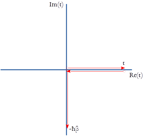
(a) Standard correlation function, Eq. 1

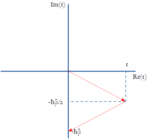
(b) Complex-time correlation function, Eq. 2

Figure 1: Time contours for path integral representations of correlation functions.

The goal is to simulate correlation functions for systems interacting with $N_{\text{env}}$ uncorrelated thermal environments. The operators, $\hat{A}$ and $\hat{B}$, whose correlation function we are interested in, act on the system.

$$\hat{H} =\hat{H}_{0}+\sum_{b}^{N_{\text{env}}}\hat{H}^{(b)}_{\text{env}}$$ (4)

$$\hat{H}^{(b)}_{\text{env}} =\sum_{j}\frac{p_{j,b}^{2}}{2m_{j,b}}+\frac{1}{2}m_{j,b}\omega_{j,b}^{2}\left(x_{j,b}-\frac{c_{j,b}\hat{s}_{b}}{m_{j,b}\omega_{j,b}^{2}}\right)^{2}.$$ (5)

The $b$th bath interacts with the system through the operator $\hat{s}_{b}$. The frequencies, $\omega_{j,b}$, and couplings, $c_{j,b}$, are characterized by the spectral density,

$$J_{b}(\omega) =\frac{\pi}{2}\sum_{j}\frac{c_{j,b}^{2}}{m_{j,b}\omega_{j,b}}\delta(\omega-\omega_{j,b}).$$ (6)

For molecular or atomistic environments, the corresponding harmonic bath can be obtained through simulations of the energy-gap correlation function [51, 52].

To obtain the path integral representation for the thermal complex-time correlation function, Eq. 2, the correlation function is be expressed as follows

$$G_{\hat{A}\hat{B}}(t) =\frac{1}{Z}\Tr_{\text{sys}}\left(\hat{A}\mathbb{O}_{\hat{B}(t_{c})}\right),$$ (7)

$$\text{where }\mathbb{O}_{\hat{B}(t_{c})} =\Tr_{\text{bath}}\left(\exp(i\hat{H}t_{c}^{*}/\hbar)\hat{B}\exp(-i\hat{H}t_{c}/\hbar)\right).$$ (8)

Once we are able to simulate $\mathbb{O}_{\hat{B}(t_{c})}$ for arbitrary $\hat{B}$, $Z$ can be obtained by setting $\hat{B}$ to the identity operator.

The final path integral expression for $\mathbb{O}_{\hat{B}(t_{c})}$ for N time steps at a time point $t_{c}=N\Delta t_{c}$ is given as:

$$\matrixelement{s_{1}}{\mathbb{O}_{\hat{B}(t_{c})}}{s_{2N+2}} =\sum_{s_{2}}\sum_{s_{3}}\cdots\sum_{s_{2N+1}}\matrixelement{s_{1}}{U^{\dagger}}{s_{2}}$$

$$\times\matrixelement{s_{2}}{U^{\dagger}}{s_{3}}\cdots\matrixelement{s_{N}}{U^{\dagger}}{s_{N+1}}$$

$$\times\matrixelement{s_{N+1}}{\hat{B}}{s_{N+2}}$$

$$\times\matrixelement{s_{N+2}}{U}{s_{N+3}}\cdots\matrixelement{s_{2N}}{U}{s_{2N+1}}$$

$$\times\matrixelement{s_{2N+1}}{U}{s_{2N+2}}\times F\left[\left\{s_{j}\right\}\right]$$ (9)

$$=\sum_{s_{2}}\sum_{s_{3}}\cdots\sum_{s_{2N+1}} P^{(0)}_{s_{1},s_{2},\ldots,s_{2N+2}}F\left[\left\{s_{j}\right\}\right]$$ (10)

where $U=\exp(-i\hat{H}\Delta t_{c}/\hbar)$, $U^{\dagger}=\exp(i\hat{H}\Delta t_{c}^{*}/\hbar)$ is the short time propagator corresponding to a time step of $\Delta t_{c}=(t-i\hbar\beta/2)/N$. These bare complex-time propagators can be grouped together to form the bare path amplitude tensor, $P^{(0)}_{s_{1},s_{2},\ldots,s_{2N+2}}$. The total influence functional, $F$, is a product of the influence functionals corresponding to the each of the uncorrelated baths.

$$F\left[\left\{s_{j}\right\}\right] =\prod_{b=1}^{N_{\text{env}}}F_{b}\left[\left\{s_{j}\right\}\right]$$ (11)

$$F^{(b)}\left[\left\{s_{j}\right\}\right] =\exp\left(-\frac{1}{\hbar}\sum_{k=1}^{2N+2}\sum_{k^{\prime}=1}^{k}I^{(b)}_{kk^{\prime}}s^{(b)}_{k}s^{(b)}_{k^{\prime}}\right)$$ (12)

where $s^{(b)}_{k}$ is the eigenvalue of $\hat{s}_{b}$ corresponding to $s_{k}$. The diagonal terms of the influence functional matrix are

$$I^{(b)}_{kk} =\frac{2}{\pi}\int_{0}^{\infty}\differential\omega\frac{J(\omega)}{\omega^{2}\sinh(\hbar\beta\omega/2)}$$

$$\times\sin\left(\omega\left(\frac{t_{k+1}-t_{k}-i\hbar\beta}{2}\right)\right)\sin\left(\omega\left(\frac{t_{k+1}-t_{k}}{2}\right)\right)$$ (13)

and the off-diagonal terms are

$$I^{(b)}_{kk^{\prime}} =\frac{4}{\pi}\int_{0}^{\infty}\differential\omega\frac{J(\omega)}{\omega^{2}\sinh(\hbar\beta\omega/2)}$$

$$\times\cos\left(\omega\left(\frac{t_{k+1}+t_{k}-t_{k^{\prime}+1}-t_{k^{\prime}}-i\hbar\beta}{2}\right)\right)$$

$$\times\sin\left(\omega\left(\frac{t_{k+1}-t_{k}}{2}\right)\right)\sin\left(\omega\left(\frac{t_{k+1}-t_{k}}{2}\right)\right),$$ (14)

when $k\neq k^{\prime}$ [24, 25]. This symmetric $I^{(b)}$-matrix is a discretization of the complex-time bath response function:

$$\alpha^{(b)}(\tau) =\sum_{j}\frac{c_{j,b}^{2}}{2m_{j,b}\omega_{j,b}}\frac{\cos\left(\omega_{j}(\tau+i\frac{\hbar\beta}{2})\right)}{\sinh\left(\frac{\hbar\beta\omega_{j}}{2}\right)}$$ (15)

$$=\frac{1}{\pi}\int_{0}^{\infty}\differential\omega J_{b}(\omega)\frac{\cos\left(\omega(\tau+i\frac{\hbar\beta}{2})\right)}{\sinh\left(\frac{\hbar\beta\omega}{2}\right)}$$ (16)

along the contour shown in Fig. 1 (b). As observed by  Shao and Makri [27] the response function is maximum in the neighborhood of $t_{c}=0$ and $t_{c}=-i\hbar\beta$. Unlike the real time bath correlation function [53], though the complex-time $\alpha$ is finite everywhere, it does not decay with increasing $\mid t_{c}\mid$. However, notice that $\alpha$ decays as $\real(t_{c})\to\infty$ and as $\imaginary(t_{c})\to-i\hbar\beta/2$. The goal is to use this localization of non-Markovian interactions to generate compact tensor network representations of the path amplitude tensor.

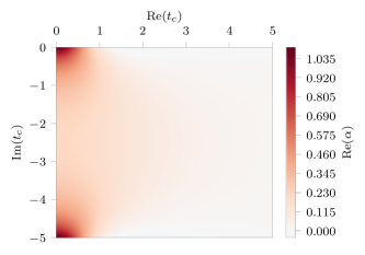
(a) Real part of $\alpha$.

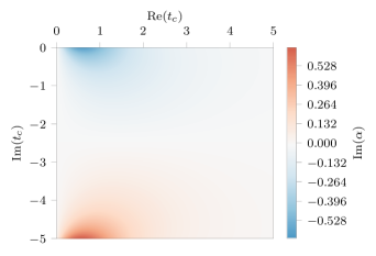
(b) Imaginary part of $\alpha$.

Figure 2: Bath response function $\alpha$ as a function of complex time for an Ohmic spectral density with $\xi=2$ and $\omega_{c}=1$ at an inverse temperature of $\beta=5$.

To begin the process observe that the bare path amplitude tensor only connects the nearest neighbors. Consequently, a matrix product representation of this tensor should be highly efficient. Consider the singular value factorizations of $U$, $U^{\dagger}$ and $\hat{B}$:

$$U^{\dagger}_{s_{j},s_{j+1}} =\sum_{\alpha_{j}}L^{(\text{back})}_{s_{j},\alpha_{j}}R^{(\text{back})}_{\alpha_{j},s_{j+1}}$$ (17)

$$U_{s_{j},s_{j+1}} =\sum_{\alpha_{j}}L^{(\text{for})}_{s_{j},\alpha_{j}}R^{(\text{for})}_{\alpha_{j},s_{j+1}}$$ (18)

$$\hat{B}_{s_{N+1},s_{N+2}} =\sum_{\alpha_{N+1}}B^{(L)}_{s_{N+1},\alpha_{N+1}}B^{(R)}_{\alpha_{N+1},s_{N+2}}$$ (19)

In the above expressions, the singular value matrices have been absorbed into either the left or the right matrix. These factorized forms can be reassembled to create the matrix product state representation of the bare path amplitude tensor as follows:

$$P^{(0)}_{s_{1},s_{2},\ldots,s_{2N+2}} =\sum_{\{\alpha_{j}\}}M^{(1)}_{s_{1},\alpha_{1}}M^{(2)}_{\alpha_{1},s_{2},\alpha_{2}}\cdots M^{(2N+2)}_{\alpha_{2N+1},s_{2N+2}}$$ (20)

$$\text{where }M^{(1)}_{s_{1},\alpha_{1}} =L^{(\text{back})}_{s_{1},\alpha_{1}},$$ (21)

$$M^{(j)}_{\alpha_{j-1},s_{j},\alpha_{j}} =R^{(\text{back})}_{\alpha_{j-1},s_{j}}L^{(\text{back})}_{s_{j},\alpha_{j}},2\leq j\leq N,$$ (22)

$$M^{(N+1)}_{\alpha_{N},s_{N+1},\alpha_{N+1}} =R^{(\text{back})}_{\alpha_{N},s_{N+1}}B^{(L)}_{s_{N+1},\alpha_{N+1}},$$ (23)

$$M^{(N+2)}_{\alpha_{N+1},s_{N+2},\alpha_{N+2}} =B^{(R)}_{\alpha_{N+1},s_{N+2}}L^{(\text{for})}_{s_{N+2},\alpha_{N+2}},$$ (24)

$$M^{(j)}_{\alpha_{j-1},s_{j},\alpha_{j}} =R^{(\text{for})}_{\alpha_{j-1},s_{j}}L^{(\text{for})}_{s_{j},\alpha_{j}},N+3\leq j\leq 2N+1,$$ (25)

$$M^{(2N+2)}_{\alpha_{2N+1},s_{2N+2}} =R^{(\text{for})}_{\alpha_{2N+1},s_{2N+2}}.$$ (26)

Here, $\alpha_{j}$ for $1\leq j\leq 2N+1$ are the bond indices and their corresponding dimensions are the so-called “bond dimensions”. Because of the nearest neighbor nature of the terms in the bare path amplitude tensor in Eq. 9, the maximum of the bond dimensions will be equal to the dimensionality of the system. The $\hat{B}$ operator has already been included in the bare path amplitude MPS at sites $N+1$ and $N+2$. The path amplitude MPS is schematically shown in Fig. 3.

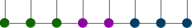
Figure 3: Path amplitude matrix product state. Green sites correspond to those with $U^{\dagger}$, purple to those with $\hat{B}$, and blue with those with $U$.

Now, the complex time influence functional needs to be incorporated. In order to accomplish this, we refactorize the total influence functional, Eq. 11, as a constrained product of terms representing interactions of one specific site, say $k$, with all other sites,

$$F_{k}\left[\left\{s_{j}\right\}\right] =\exp\left(-\frac{1}{\hbar}\sum_{k^{\prime}=1}^{2N+2}\sum_{b=1}^{N_{\text{env}}}I^{(b)}_{kk^{\prime}}s^{(b)}_{k}s^{(b)}_{k^{\prime}}\right).$$ (27)

In a direct implementation, there will be a double counting of every interaction in the product of terms like Eq. 27. This double counting of interactions is avoided by tracing over the $k$th site immediately after applying $F_{k}$. The “constrain” is that the sum over $k^{\prime}$ in Eq. 27 will happen over the existing sites only. As a consequence, now when we move to, say, site $k+1$, $F_{k+1}$ will not include the interaction between $k$ and $k+1$ because that has already been incorporated in the previous step. The procedure will be continued for the next chosen site. To be able to do this, there are two necessary problems that we have to solve: (1) we need to be able to provide a matrix product representation for the interaction of all sites with the $k$th site, and (2) we need to come up with an ordering of the sites that minimizes the computational and storage requirements. In this, sites 1 and $2N+2$ will not be traced over as they are required for the matrix representation of $\mathbb{O}_{\hat{B}(t_{c})}$ and subsequent multiplication with $\hat{A}$.

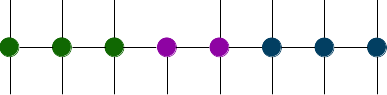
Figure 4: Schematic of the first influence functional operator applied to the path amplitude MPS. The colors are only for helping synchronize this schematic with Fig. 3. Note that the site for which all interactions are included does not have an upper edge indicating an automatic trace over the coordinate.

Let us start with the second problem: assuming that we can represent the influence functional operator of all the interactions with site $j$, how do we order the application of these operators for maximal efficiency? Are there orderings that are better than others? As discussed, Fig. 2 demonstrates a decay of correlation as $\real(t_{c})$ increases and $\imaginary(t_{c})\to-i\hbar\beta/2$. So, if we started applying the operator from site 2 and tracing it out, the correlations would initially decrease till $\imaginary(t_{c})=-i\hbar\beta/2$ but then increase till the end of the contour where $\imaginary(t_{c})=-i\hbar\beta$. These highly non-local interactions, that do not decay monotonically with distance along the complex time contour, would make the bond dimensions of the MPS grow very quickly on application of the influence functional MPO. However, we can try to apply the influence functional operators in pairs from the middle outwards. This has the advantage of making the non-local interactions “look” short-ranged, and consequently prevents the spurious growth of bond dimension in any other ordering. In fact, given the structure of $\alpha$, going from $t_{c}=-i\hbar\beta/2$ outwards towards $t_{c}=0$ and $t_{c}=-i\hbar\beta$ is computationally the most optimal order of incorporation of the influence functional.

We will think in terms of multiple steps of incorporation of the influence functional, with each step consisting of incorporation of the non-Markovian interactions involving the middle two points. So, the first operator applied would take care of all non-Markovian interactions with site $N+1$ and tracing over it. A schematic of this is shown in Fig. 4. This is not a typical matrix product operator (MPO). A key difference being that MPOs have the same number of downward and upward site indices. Here, the site whose interactions are being taken into account does not have an upward index. Consequently, the output MPS after application of the influence functional operator has one site less. On application of this operator to the bare path amplitude MPS will result in an MPS with one less site.

After application of the first influence functional operator, site number $N+1$ ceases to exist. (To keep simplify our nomenclature, we will keep using the original numbering. So, though site $N+2$ which has the information from the $\hat{B}$ operator is now the $(N+1)$th site, we will still refer to it as site $N+2$. There is no site $N+1$ now.) Then the influence functional corresponding to site number $N+2$ will be applied, with that site being traced over. (The influence functional corresponding to the $N+2$ will not contain the interactions between the $N+2$th site and the $N+1$th site because this has been incorporated already before tracing over the latter. In this fashion, every subsequent influence functional will only consist of interactions between the sites that still exist.) This completes the first step of incorporation of the non-Markovian influence functional. Sites $N$ and $N+3$ would be incorporated in the second step, $N-1$ and $N+4$ in the third, so on and so forth till site $2$ and $2N+1$ are incorporated. The first couple of steps of the influence functional application is schematically shown in Fig. 5.

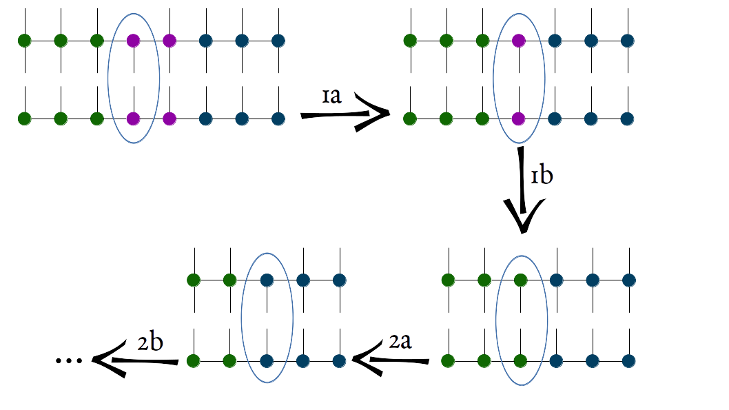
Figure 5: First few steps of application of the influence functional operators. On application of the influence functional operator to the MPS, there is always one site with no dangling edges (no site index). This internal site is absorbed into the site that is left to it.

Having analyzed the structure of the non-Markovian memory and the order of application of the operators, we now derive the matrix-product representation for the complex-time influence functional connecting all the sites to a particular site $k$ (for $2\leq k\leq 2N+1$). During the steps of application of the influence functional operators, we trace out sites from the middle of the contour. Let $l<k$ be the last remaining site to the left of the site $k$, and $r>k$ be the first site immediately to the right of site $k$. At this stage of application, all the sites to the left of $l$ ($j\leq l$) and right of $r$ ($j\geq r$) must exist.

$$F_{k}\left[\left\{s_{j}\right\}\right] =\sum_{\{\beta_{j}\}}\mathcal{F}^{(1)}_{s_{1},s_{1}^{\prime},\beta_{1}}\mathcal{F}^{(2)}_{\beta_{1},s_{2},s_{2}^{\prime},\beta_{2}}\cdots$$

$$\times\mathcal{F}^{(l)}_{\beta_{l-1},s_{l},s_{l}^{\prime},\beta_{l}}\mathcal{F}^{(k)}_{\beta_{l},s_{k},\beta_{r-1}}\mathcal{F}^{(r)}_{\beta_{r-1},s_{r},s_{r}^{\prime},\beta_{r}}$$

$$\times\cdots\mathcal{F}^{(2N+1)}_{\beta_{2N},s_{2N+1},s_{2N+1}^{\prime},\beta_{2N+1}}\mathcal{F}^{(2N+2)}_{\beta_{2N+1},s_{2N+2},s_{2N+2}^{\prime}}$$ (28)

Notice that the tensor with index $k$ has only one unprimed site index. This is the feature that enables the automatic tracing over the $k$th site and is shown in Fig. 4. The exact forms of the constituent tensors, $\mathcal{F}$ are listed in the Appendix A.

Now, we can define the complete algorithm for simulating the correlation function at a time point $N\Delta t$ is as follows:

• Obtain the bare path amplitude MPS corresponding to $\mathbb{O}_{B(t_{c})}$ with $2N+2$ sites.

• Apply the influence functional operator corresponding to $F_{N+1}$ which encodes all the interactions with the $(N+1)$th time point along the complex time contour.

• Apply $F_{N+2}$. This completes the first step of the application of the influence functional and now the path amplitude MPS has $2N$ sites. (We are still following our convention of retaining the time labels of the points.)

• Apply $F_{N}$ and $F_{N+3}$. Path amplitude MPS now has $2N-2$ sites.

• Repeat till path amplitude MPS has just 2 sites.

• Contract this 2-site MPS into a matrix and apply the influence functional between sites 1 and $2N+2$.

• Multiply by $\hat{A}$ and trace to get the correlation function.

The computational complexity of any MPS-based method is determined by the maximum bond dimension of the MPS [32, 35]. Though the current CT-TNPI algorithm is not based on conventional MPO-MPS applications, the same arguments and ideas go through. For every final time point, we have multiple influence functional operators acting on the path amplitude MPS in sequence leading to a possible increase in the maximum bond dimension. We define $\bar{\beta}(t)$ as the average of the maximum bond dimensions encountered over simulation for a particular time, $t$. This measure governs the computational requirements of the method. Various common optimizations and singular value-based filtering schemes that are used in regular MPO-MPS application can be used here as well. These are typically governed by two convergence parameters: the cutoff threshold governing the truncated singular value decomposition and the maximum bond dimension of the resulting MPS. Variational procedures may also be used for applying the influence functional operator to the path amplitude MPS.

III Results

As numerical illustrations of the method, we provide examples from rate theory, calculations of spin correlation functions and susceptibilities and some thermodynamics of the Fenna–Mathhews–Olson complex of photosynthesis. For the first two sets of examples the system under study can be simply described by a symmetric spin-half particle or a two-level Hamiltonian:

$$\hat{H}_{0} =-\hbar\Omega\sigma_{x},$$ (29)

where $\sigma_{j}$ for $j$ in $\left\{x,y,z\right\}$ are the spin-1/2 Pauli matrices. There is one bath that couples to the system through the $\sigma_{z}$ operator. In these model problems, the spectral density of the bath is taken to be of the general form:

$$J(\omega) =\frac{\pi}{2}\hbar\xi\omega^{s}\omega_{c}^{1-s}\exp\left(-\frac{\omega}{\omega_{c}}\right),$$ (30)

where $\omega_{c}$ is the characteristic frequency of the bath and $\xi$ is the dimensionless Kondo parameter encoding the strength of the system-environment coupling. The parameter $s$ decides the nature of the spectral density, with $s=1$ being the celebrated Ohmic form.

III.1 Rate theory

For the first example consider calculation of reaction rates. Many reactions happen at significantly slower time scales compared to the ro-translational motion of the reactants. In such cases, it becomes difficult to directly simulate the reaction, and one often resorts to calculations of reaction rates. While reaction rates can be calculated classically, such approaches miss out on quantum effects of nuclei, and are generally unsuitable for purely non-adiabatic reactions like electron transport. It has been shown that the rate of a reaction is linked to the improper integral of the flux-flux correlation function over all time, or the zero frequency component of the spectrum corresponding to the flux-flux correlation function: [4, 5, 6, 7]

$$k =\int_{0}^{\infty}C_{ff}(t)$$ (31)

$$C_{ff}(t) =\frac{1}{Q}\Tr\left(F\exp\left(i\frac{\hat{H}t_{c}^{*}}{\hbar}\right)F\exp\left(-i\frac{\hat{H}t_{c}}{\hbar}\right)\right),$$ (32)

where $Q$ is the reactant partition function and $F=\frac{i}{\hbar}\commutator{\hat{H}}{\outerproduct{R}{R}}$ is the flux operator. An equivalent formulation can be built in terms of the long-time limit of the so-called “flux-side” correlation, which is the integral of the flux-flux correlation function: [6, 7]

$$k =\lim_{t\to\infty}C_{fs}(t)$$ (33)

$$C_{fs}(t) =\frac{1}{Q}\Tr\left(F\exp\left(i\frac{\hat{H}t_{c}^{*}}{\hbar}\right)\outerproduct{R}{R}\exp\left(-i\frac{\hat{H}t_{c}}{\hbar}\right)\right).$$ (34)

In condensed phase reactions, the infinite time limits in both the equations can be truncated to a plateau time $t_{\text{plateau}}$ after which the flux-side correlation function becomes constant and the flux-flux correlation function becomes zero.

One can think of the rate as half of the zero frequency component of a frequency-dependent rate function corresponding to the flux-flux autocorrelation function. [23] These quantum flux-based reaction rates have been simulated not just using equilibrium correlation functions, approaches of using non-equilibrium [29] and near-equilibrium simulations [30] have also been shown to give the correct rates.

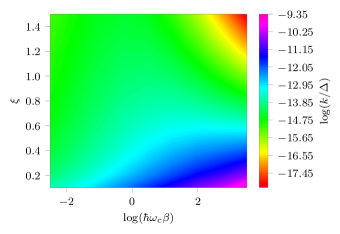
(a) $s=1$

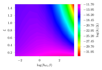
(b) $s=0.5$

Figure 6: Rates of reaction for a symmetric two-state system normalized to the tunneling splitting.

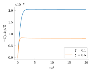
(a) Flux-side correlation function

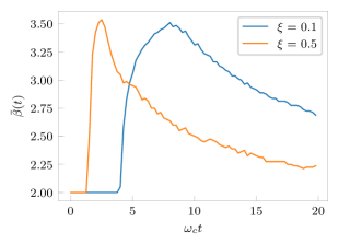
(b) Bond dimension as a function of time

Figure 7: Simulations for $\hbar\omega_{c}\beta=0.2$. Both flux-side correlation function and the values of $\bar{\beta}(t)$ shown for two different system-solvent couplings of $\xi=0.1$ and $\xi=0.5$.

Consider a two-state model for symmetric proton transfer process where the tunneling splitting is much smaller than the vibronic frequencies. This separation of time scales, common in many reactions, is critical to the applicability of rate theory. Following Topaler and Makri [25], consider a symmetric two-state system with a tunneling splitting of $\Delta=2\hbar\Omega=$0.001\,05\text{\,}{\mathrm{cm}}^{-1}$$. The environment considered has the form given in Eq. 30 with a high cutoff frequency of $\omega_{c}=$500\text{\,}{\mathrm{cm}}^{-1}$$. We investigate the rates for the Ohmic case ($s=1$) which is ubiquitous for condensed phase systems, a sub-Ohmic case ($s=0.5$), and a super-Ohmic case ($s=3$) which is useful for modeling phonons in three dimensional solids. The rates for a range of temperatures and coupling strengths are shown in Fig. 6. The simulation parameters used in these cases were much more than what is necessary for convergence. The data shown in Fig. 6 correspond to $N=30$ and a cutoff threshold of $10^{-20}$.

To demonstrate the performance of the CT-TNPI method, we plot the flux-side correlation function and $\bar{\beta}(t)$ for two particular parameters in Fig. 7. These calculations were run with $N=40$ and a cutoff threshold of $10^{-20}$. Despite this, $\bar{\beta}(t)$ is very small throughout the period of simulation demonstrating the efficiency of the method. The magnitudes of $\bar{\beta}(t)$ is often dependent on the particular correlation function as we will numerically demonstrate in the next examples.

III.2 Symmetrized spin correlation functions

One of the dynamical quantities of interest for the spin-boson model is the symmetrized spin correlation function (SSCF) [9, 19]. For a generic spin operator, $\sigma$, the SSCF, defined as

$$S(t) =\frac{1}{2Z}\Tr\left(\exp(-\beta\hat{H})\left(\sigma(t)\sigma(0)+\sigma(0)\sigma(t)\right)\right),$$ (35)

is related to the structure factor [1]. The spectrum of SSCF is related to the spectrum of the complex-time correlation function as

$$S(\omega) =\cosh\left(\frac{\hbar\omega\beta}{2}\right)G(\omega),$$ (36)

where $G(\omega)=\int_{-\infty}^{\infty}G(t)\exp(i\omega t)\differential t$.

Additionally, the Fourier transform of the imaginary part of the dynamical susceptibility,

$$\chi(t) =\frac{i\Theta(t)}{Z}\Tr\left(\exp(-\beta\hat{H})\left(\sigma(t)\sigma(0)-\sigma(0)\sigma(t)\right)\right).$$ (37)

is also related to the spectrum of SSCF. This along with Kramer-Kronig’s relation allow us to estimate both the real ($\chi^{\prime}(\omega)$) and the imaginary ($\chi^{\prime\prime}(\omega)$) parts of $\chi(\omega)$. Thus, combining all these relations, it is possible to calculate the symmetrized correlation function as well as the dynamical susceptibility for open quantum systems directly with the CT-TNPI.

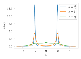
(a) Weakly coupled bath with $\xi=0.03$.

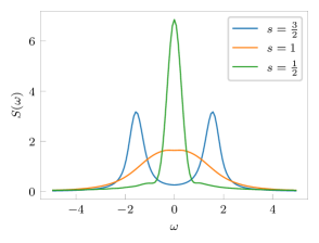
(b) Strongly coupled bath with $\xi=0.18$.

Figure 8: Comparison of spectra corresponding to SSCF of system coupled with Ohmic and non-Ohmic baths of different strengths.

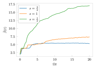
Figure 9: Bond dimension for different baths with Kondo parameter, $\xi=0.03$.

Consider a symmetric spin-boson Hamiltonian with a tunneling splitting $2\hbar\Omega=2$ connected to a spectral density given by Eq. 30 with a high cutoff frequency of $\omega_{c}=30\Omega$ held at a temperature of $\hbar\Omega\beta=0.4$. We study SSCF for three different kinds of spectral densities defined by the value of $s$: we look at the Ohmic spectral density ($s=1$), a sub-Ohmic spectral density ($s=0.5$), and a super-Ohmic spectral density ($s=1.5$). The SSCF spectra are shown in Fig. 8 for two different Kondo parameters $\xi$. The correlation functions were converged for the time span under consideration with $N=30$ steps and a cutoff threshold of $10^{-10}$. As we go from sub- to Ohmic to super-Ohmic, the oscillatory character of the dynamics, represented by the well-separated peaks of the SSCF spectrum, increases. The bond dimensions as characterized by $\bar{\beta}(t)$ for all the three baths at a Kondo parameter of $\xi=0.03$ is shown in Fig. 9. Notice that in addition to the sub-Ohmic bath being the most efficient at dissipating the oscillatory dynamics, it also leads to the fastest growth of $\bar{\beta}(t)$.

In Fig. 10, we track the real and imaginary parts of the dynamical suscpetibility at different system-solvent coupling strength for the Ohmic and sub-Ohmic ($s=0.5$) cases. Notice the faster loss of coherent oscillations in the sub-Ohmic spectral density gets reflected here as well. The frequency dependencies of the susceptibilities are extremely dependent on the spectral density of the bath. Because the path integral calculations are non-perturbative, unlike other approximations [9, 54], the current approach gives the correct result at all parameters upon systematic convergence.

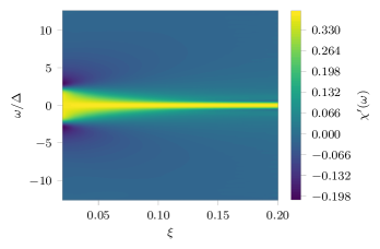
(a) $\chi^{\prime}(\omega)$ for sub-Ohmic spectral density ($s=0.5$).

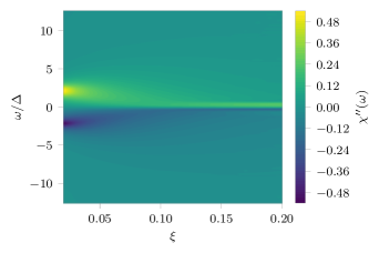
(b) $\chi^{\prime\prime}(\omega)$ for sub-Ohmic spectral density ($s=0.5$).

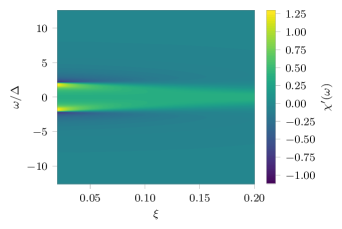
(c) $\chi^{\prime}(\omega)$ for Ohmic spectral density ($s=1$).

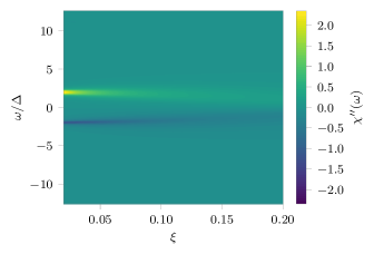
(d) $\chi^{\prime\prime}(\omega)$ for Ohmic spectral density ($s=1$).

Figure 10: Dynamical susceptibility for a spin-boson system for different bath spectral densities.

III.3 Thermodynamics

As a final example consider the equilibrium density matrices of corresponding to the single excitation subspace in the Fenna–Matthews–Olson complex (FMO) at an ambient temperature of $T=$300\text{\,}\mathrm{K}$$. FMO is typically a trimer of octamers of chlorophyll molecules. Here we consider only one unit of the trimer. The system Hamiltonian is given as

$$\hat{H}_{0} =\sum_{j}\epsilon_{j}\outerproduct{j}{j}+\sum_{j}\sum_{l\neq j}h_{jl}\left(\outerproduct{j}{l}+\outerproduct{l}{j}\right),$$ (38)

where $\epsilon_{j}$ is the excitation energy of the $j$th chlorophyll molecule, $h_{jl}$ is the electronic coupling between the excited state of the $j$th molecule and the ground state of the $l$th molecule. The basis $\ket{j}$ corresponds to the $j$th molecule being in the excited state and all other molecules in the ground state.

The vibronic couplings happen through localized vibrations and shifts between the ground and excited Born-Oppenheimer states. The vibrations of the $j$th molecule have the form:

$$\hat{H}_{\text{vib}}^{(j)} =\sum_{i=1}^{N_{\text{osc}}}\frac{p_{i,j}^{2}}{2m_{i,j}}+\frac{1}{2}m_{i,j}\omega_{i,j}^{2}\left(x_{i,j}-\frac{c_{i,j}\outerproduct{j}{j}}{m_{i,j}\omega_{i,j}^{2}}\right)^{2}.$$ (39)

The system Hamiltonian and vibronic degrees of freedom are difficult to characterize. However recent work [55] has provided some ab initio QM/MM level simulations of the spectral densities and the system Hamiltonians. These descriptions have also been used to study the excitonic dynamics and pathways of transport [47, 48].

The equilibrium density matrices corresponding to the single excitation sector is shown in Fig. 11. Because of differences in the system Hamiltonian and vibronic couplings, the equilibrium density matrices shown in Fig. 11 are completely different. It is interesting that the difference also shows up in the purity of the thermal ensemble with the ZINDO equilibrium being significantly more pure ($\Tr(\rho^{2})=0.938$) than the TD-LC-DFTB equilibrium density matrix ($\Tr(\rho^{2})=0.63$). The von Neumann entropies are also very different with ZINDO having very low entropy at 0.174 and TD-LC-DFTB being considerably more entangled at 0.91.

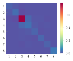
(a) TD-LC-DFTB parameterization.

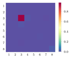
(b) ZINDO parameterization.

Figure 11: Equilibrium density matrix for FMO under different parameterizations at $T=$300\text{\,}\mathrm{K}$$.

IV Conclusion

Equilibrium correlation functions form the basis for simulations of various experimentally relevant observables. When open quantum systems are involved, these correlation functions become to simulate because of an exponential scaling of computational complexity with number of degrees of freedom. Path integrals and influence functional provide a lucrative way of rigorously incorporating influence of baths in these non-Markovian simulations. However as the number of paths increase, both the computational and storage requirements tend to scale exponentially.

Tensor network is a commonly-used framework of generating compact representations of tensors with large orders. Wide-ranging applications of tensor networks about in physics [31, 34, 36, 35] and chemistry [56, 57, 58]. In this article, we present a tensor network-based approach to simulation of thermal correlation functions for open quantum systems. A matrix product state is used to provide a compressed representation for the path ampltiude tensor. We show that the non-Markovian correlations for the complex-time influence functional do not decay monotonically with the history. So, if the influence functional is naïvely represented as a matrix product operator, the path amplitude MPS will not offer optimal compression. We use the structure of the bath response function to motivate an order of applying the influence functional that minimizes the growth of bond dimension and consequently is optimal from a computational perspective. Computationally, the tensor network backend opens up possibilities of future use of graphics processing units to further accelerate simulations.

Various examples from rate theory, thermodynamics and spin correlation functions have been used to illustrate the efficiency and broad applicability of the method. In the near future, we will focus on comparing vibrational dynamics of small molecules and rates of more complicated reactions in bulk and inside a cavity. Beyond these system specific studies, this work forms the first step in forming an infrastructure for multitime correlation functions that leverages tensor networks for greater efficiency. Such multitime correlation functions are related to various multidimensional spectra [3]. Furthermore, the flexibility of the tensor network approaches allow us the ability to explore routes to equilibration starting from non-equilibrium initial conditions. Finally, the complex time tensor network path integral code developed in Julia [59] using the ITensor [60, 61] will be released soon as a part of the QuantumDynamics.jl [62] library that was recently introduced as a platform for simulating dynamics in open quantum systems using various methods.

Appendix A Influence Functional Operators

Below are the exact forms of the constituent tensors of the matrix product influence functional operator.

$$\mathcal{F}^{(k)}_{\beta_{l},s_{k},\beta_{r-1}} =\delta_{\beta_{l},s_{k}}\delta_{\beta_{r-1},s_{k}}\exp\left(-\frac{1}{\hbar}\sum_{b=1}^{N_{\text{env}}}I^{(b)}_{kk}s^{(b)}_{k}s^{(b)}_{k}\right)$$ (40)

$$\mathcal{F}^{(k^{\prime})}_{\beta_{k^{\prime}-1},s_{k^{\prime}},\beta_{k^{\prime}}} =\delta_{\beta_{k^{\prime}-1},\beta_{k^{\prime}}}\exp\left(-\frac{1}{\hbar}\sum_{b=1}^{N_{\text{env}}}I^{(b)}_{kk^{\prime}}\beta^{(b)}_{k^{\prime}}s^{(b)}_{k^{\prime}}\right)$$ (41)

$$\mathcal{F}^{(1)}_{s_{1},\beta_{1}} =\exp\left(-\frac{1}{\hbar}\sum_{b=1}^{N_{\text{env}}}I^{(b)}_{1k}\beta^{(b)}_{1}s^{(b)}_{1}\right)$$ (42)

$$\mathcal{F}^{(2N+2)}_{\beta_{2N+1},s_{2N+2}} =\exp\left(-\frac{1}{\hbar}\sum_{b=1}^{N_{\text{env}}}I^{(b)}_{k,2N+2}\beta^{(b)}_{2N+1}s^{(b)}_{2N+2}\right)$$ (43)

On application of the influence functional operators, the number of sites on the path amplitude MPS decreases by one. The extra vertex that is left behind without a site index is absorbed conventionally in the vertex that is immediately to the right. With these definitions, we have a complete definition of the tensor networks required to simulate complex time correlation functions in a manner that optimally uses the structure of the complex-time bath response function.

References

- Weiss [2012] U. Weiss, Quantum Dissipative Systems, 3rd ed. (World Scientific, 2012).
- Schuricht and Schoeller [2009] D. Schuricht and H. Schoeller, “Dynamical spin-spin correlation functions in the Kondo model out of equilibrium,” Phys. Rev. B 80, 075120 (2009).
- Mukamel [1995] S. Mukamel, Principles of Nonlinear Optical Spectroscopy, Oxford Series in Optical and Imaging Sciences No. 6 (Oxford University Press, New York, 1995).
- Kubo [1957] R. Kubo, “Statistical-Mechanical Theory of Irreversible Processes. I. General Theory and Simple Applications to Magnetic and Conduction Problems,” Journal of the Physical Society of Japan 12, 570–586 (1957).
- Yamamoto [1960] T. Yamamoto, “Quantum Statistical Mechanical Theory of the Rate of Exchange Chemical Reactions in the Gas Phase,” The Journal of Chemical Physics 33, 281–289 (1960).
- Miller [1974] W. H. Miller, “Quantum mechanical transition state theory and a new semiclassical model for reaction rate constants,” The Journal of Chemical Physics 61, 1823–1834 (1974).
- Miller, Schwartz, and Tromp [1983] W. H. Miller, S. D. Schwartz, and J. W. Tromp, “Quantum mechanical rate constants for bimolecular reactions,” The Journal of Chemical Physics 79, 4889–4898 (1983).
- Liu and Miller [2007] J. Liu and W. H. Miller, “Real time correlation function in a single phase space integral beyond the linearized semiclassical initial value representation,” The Journal of Chemical Physics 126, 234110 (2007), https://doi.org/10.1063/1.2743023 .
- Liu, Xu, and Wu [2016] J. Liu, H. Xu, and C.-Q. Wu, “Green’s functions for spin boson systems: Beyond conventional perturbation theories,” Chemical Physics 481, 42–53 (2016).
- Wang, Thoss, and Miller [2000] H. Wang, M. Thoss, and W. H. Miller, “Forward–backward initial value representation for the calculation of thermal rate constants for reactions in complex molecular systems,” The Journal of Chemical Physics 112, 47–55 (2000), https://doi.org/10.1063/1.480560 .
- Wang, Thoss, and Miller [2001] H. Wang, M. Thoss, and W. H. Miller, “Systematic convergence in the dynamical hybrid approach for complex systems: A numerically exact methodology,” J. Chem. Phys. 115, 2979–2990 (2001).
- Miller [2006] W. H. Miller, “Including quantum effects in the dynamics of complex (i.e., large) molecular systems,” The Journal of Chemical Physics 125, 132305 (2006).
- Cao and Voth [1994a] J. Cao and G. A. Voth, “The formulation of quantum statistical mechanics based on the Feynman path centroid density. I. Equilibrium properties,” The Journal of Chemical Physics 100, 5093–5105 (1994a).
- Cao and Voth [1994b] J. Cao and G. A. Voth, “The formulation of quantum statistical mechanics based on the Feynman path centroid density. II. Dynamical properties,” The Journal of Chemical Physics 100, 5106–5117 (1994b).
- Craig and Manolopoulos [2004] I. R. Craig and D. E. Manolopoulos, “Quantum statistics and classical mechanics: Real time correlation functions from ring polymer molecular dynamics,” The Journal of Chemical Physics 121, 3368–3373 (2004).
- Habershon et al. [2013] S. Habershon, D. E. Manolopoulos, T. E. Markland, and T. F. Miller, “Ring-polymer molecular dynamics: Quantum effects in chemical dynamics from classical trajectories in an extended phase space,” Annual Review of Physical Chemistry 64, 387–413 (2013), https://doi.org/10.1146/annurev-physchem-040412-110122 .
- Florens et al. [2011] S. Florens, A. Freyn, D. Venturelli, and R. Narayanan, “Dissipative spin dynamics near a quantum critical point: Numerical renormalization group and Majorana diagrammatics,” Phys. Rev. B 84, 155110 (2011).
- Schad et al. [2015] P. Schad, Yu. Makhlin, B. Narozhny, G. Schön, and A. Shnirman, “Majorana representation for dissipative spin systems,” Annals of Physics 361, 401–422 (2015).
- Schad [2016] P. Schad, On the Majorana Representation for Spin 1/2, Ph.D. thesis, Karlsruher Institut fur Technologie (2016).
- Dekker [1987] H. Dekker, “Noninteracting-blip approximation for a two-level system coupled to a heat bath,” Phys. Rev. A 35, 1436–1437 (1987).
- Leggett et al. [1987] A. J. Leggett, S. Chakravarty, A. T. Dorsey, M. P. A. Fisher, A. Garg, and W. Zwerger, “Dynamics of the dissipative two-state system,” Rev. Mod. Phys. 59, 1–85 (1987).
- Rabani, Krilov, and Berne [2000] E. Rabani, G. Krilov, and B. J. Berne, “Quantum mechanical canonical rate theory: A new approach based on the reactive flux and numerical analytic continuation methods,” J. Chem. Phys. 112, 2605–2614 (2000).
- Sim, Krilov, and Berne [2001] E. Sim, G. Krilov, and B. J. Berne, “Quantum Rate Constants from Short-Time Dynamics: An Analytic Continuation Approach,” J. Phys. Chem. A 105, 2824–2833 (2001).
- Topaler and Makri [1993] M. Topaler and N. Makri, “Quasi-adiabatic propagator path integral methods. Exact quantum rate constants for condensed phase reactions,” Chemical Physics Letters 210, 285–293 (1993).
- Topaler and Makri [1994] M. Topaler and N. Makri, “Quantum rates for a double well coupled to a dissipative bath: Accurate path integral results and comparison with approximate theories,” The Journal of Chemical Physics 101, 7500–7519 (1994).
- Topaler and Makri [1996] M. Topaler and N. Makri, “Path Integral Calculation of Quantum Nonadiabatic Rates in Model Condensed Phase Reactions,” J. Phys. Chem. 100, 4430–4436 (1996).
- Shao and Makri [2001] J. Shao and N. Makri, “Iterative path integral calculation of quantum correlation functions for dissipative systems,” Chemical Physics 268, 1–10 (2001).
- Shao and Makri [2002] J. Shao and N. Makri, “Iterative path integral formulation of equilibrium correlation functions for quantum dissipative systems,” J. Chem. Phys. 116, 507–514 (2002).
- Bose and Makri [2017] A. Bose and N. Makri, “Non-equilibrium reactive flux: A unified framework for slow and fast reaction kinetics,” The Journal of Chemical Physics 147, 152723 (2017).
- Bose and Makri [2019] A. Bose and N. Makri, “Quasiclassical Correlation Functions from the Wigner Density Using the Stability Matrix,” Journal of Chemical Information and Modeling 59, 2165–2174 (2019).
- White [1992] S. R. White, “Density matrix formulation for quantum renormalization groups,” Physical Review Letters 69, 2863–2866 (1992).
- Schollwöck [2011a] U. Schollwöck, “The density-matrix renormalization group in the age of matrix product states,” Annals of Physics 326, 96–192 (2011a).
- Schollwöck [2011b] U. Schollwöck, “The density-matrix renormalization group: A short introduction,” Philosophical Transactions of the Royal Society A: Mathematical, Physical and Engineering Sciences 369, 2643–2661 (2011b).
- White and Feiguin [2004] S. R. White and A. E. Feiguin, “Real-Time Evolution Using the Density Matrix Renormalization Group,” Physical Review Letters 93, 076401 (2004).
- Paeckel et al. [2019] S. Paeckel, T. Köhler, A. Swoboda, S. R. Manmana, U. Schollwöck, and C. Hubig, “Time-evolution methods for matrix-product states,” Annals of Physics 411, 167998 (2019).
- White [2009] S. R. White, “Minimally entangled typical quantum states at finite temperature,” Phys. Rev. Lett. 102, 190601 (2009).
- Strathearn et al. [2018] A. Strathearn, P. Kirton, D. Kilda, J. Keeling, and B. W. Lovett, “Efficient non-Markovian quantum dynamics using time-evolving matrix product operators,” Nature Communications 9, 3322 (2018).
- Jørgensen and Pollock [2019] M. R. Jørgensen and F. A. Pollock, “Exploiting the Causal Tensor Network Structure of Quantum Processes to Efficiently Simulate Non-Markovian Path Integrals,” Physical Review Letters 123, 240602 (2019).
- Bose and Walters [2021] A. Bose and P. L. Walters, “A tensor network representation of path integrals: Implementation and analysis,” arXiv pre-print server arXiv:2106.12523 (2021), arxiv:2106.12523 .
- Bose and Walters [2022a] A. Bose and P. L. Walters, “A multisite decomposition of the tensor network path integrals,” The Journal of Chemical Physics 156, 024101 (2022a).
- Bose [2022a] A. Bose, “Pairwise connected tensor network representation of path integrals,” Physical Review B 105, 024309 (2022a).
- Cerrillo and Cao [2014] J. Cerrillo and J. Cao, “Non-Markovian Dynamical Maps: Numerical Processing of Open Quantum Trajectories,” Phys. Rev. Lett. 112, 110401 (2014).
- Makri [2018] N. Makri, “Modular path integral methodology for real-time quantum dynamics,” The Journal of Chemical Physics 149, 214108 (2018).
- Makri [2020] N. Makri, “Small Matrix Path Integral for System-Bath Dynamics,” Journal of Chemical Theory and Computation 16, 4038–4049 (2020).
- Kundu and Makri [2020] S. Kundu and N. Makri, “Real-Time Path Integral Simulation of Exciton-Vibration Dynamics in Light-Harvesting Bacteriochlorophyll Aggregates,” The Journal of Physical Chemistry Letters 11, 8783–8789 (2020).
- Bose and Walters [2022b] A. Bose and P. L. Walters, “Tensor Network Path Integral Study of Dynamics in B850 LH2 Ring with Atomistically Derived Vibrations,” Journal of Chemical Theory and Computation 18, 4095–4108 (2022b).
- Bose and Walters [2023a] A. Bose and P. L. Walters, “Impact of Solvent on State-to-State Population Transport in Multistate Systems Using Coherences,” J. Chem. Theory Comput. 19, 4828–4836 (2023a).
- Bose and Walters [2023b] A. Bose and P. L. Walters, “Impact of spatial inhomogeneity on excitation energy transport in the fenna-matthews-olson complex,” arXiv pre-print server arXiv:2302.01886 (2023b), 10.48550/ARXIV.2302.01886, arxiv:2302.01886 .
- Thirumalai and Berne [1984] D. Thirumalai and B. J. Berne, “Time correlation functions in quantum systems,” The Journal of Chemical Physics 81, 2512–2513 (1984).
- Berne [1986] B. J. Berne, “Path integral Monte Carlo methods: Static- and time-correlation functions,” Journal of Statistical Physics 43, 911–929 (1986).
- Makri [1999] N. Makri, “The Linear Response Approximation and Its Lowest Order Corrections: An Influence Functional Approach,” The Journal of Physical Chemistry B 103, 2823–2829 (1999).
- Bose [2022b] A. Bose, “Zero-cost corrections to influence functional coefficients from bath response functions,” The Journal of Chemical Physics 157, 054107 (2022b).
- Makri and Makarov [1995] N. Makri and D. E. Makarov, “Tensor propagator for iterative quantum time evolution of reduced density matrices. I. Theory,” The Journal of Chemical Physics 102, 4600–4610 (1995).
- Xu and Cao [2016] D. Xu and J. Cao, “Non-canonical distribution and non-equilibrium transport beyond weak system-bath coupling regime: A polaron transformation approach,” Frontiers of Physics 11, 110308 (2016).
- Maity et al. [2020] S. Maity, B. M. Bold, J. D. Prajapati, M. Sokolov, T. Kubař, M. Elstner, and U. Kleinekathöfer, “DFTB/MM Molecular Dynamics Simulations of the FMO Light-Harvesting Complex,” The Journal of Physical Chemistry Letters 11, 8660–8667 (2020).
- Chan and Sharma [2011] G. K.-L. Chan and S. Sharma, “The Density Matrix Renormalization Group in Quantum Chemistry,” Annual Review of Physical Chemistry 62, 465–481 (2011).
- Ren, Shuai, and Kin-Lic Chan [2018] J. Ren, Z. Shuai, and G. Kin-Lic Chan, “Time-Dependent Density Matrix Renormalization Group Algorithms for Nearly Exact Absorption and Fluorescence Spectra of Molecular Aggregates at Both Zero and Finite Temperature,” Journal of Chemical Theory and Computation 14, 5027–5039 (2018).
- Olivares-Amaya et al. [2015] R. Olivares-Amaya, W. Hu, N. Nakatani, S. Sharma, J. Yang, and G. K.-L. Chan, “The ab-initio density matrix renormalization group in practice,” J. Chem. Phys. 142, 034102 (2015).
- Bezanson et al. [2017] J. Bezanson, A. Edelman, S. Karpinski, and V. B. Shah, “Julia: A fresh approach to numerical computing,” SIAM Review 59, 65–98 (2017).
- Fishman, White, and Stoudenmire [2022a] M. Fishman, S. White, and E. Stoudenmire, “The ITensor Software Library for Tensor Network Calculations,” SciPost Phys. Codebases , 4 (2022a).
- Fishman, White, and Stoudenmire [2022b] M. Fishman, S. White, and E. Stoudenmire, “Codebase release 0.3 for ITensor,” SciPost Phys. Codebases , 4–r0.3 (2022b).
- Bose [2023] A. Bose, “QuantumDynamics.jl: A modular approach to simulations of dynamics of open quantum systems,” The Journal of Chemical Physics 158, 204113 (2023).