Dataset Quantization

1 Appendix

We present more explanations of the proposed dataset quantization, experiment results and visualizations in this section.

1.1 Proof of Sec. 3.1

Given the whole dataset $\mathbf{D}$, $|\mathbf{D}|=M\gg 1$. $\forall{p}\in\mathbf{D}$, $f(p)\in\mathbb{R}^{m\times 1}$. To make a simple proof, we assume $\frac{1}{M}\sum_{p\in\mathbf{D}}f(p)=0$.

For $n=0,1,2,\cdots,n,\cdots,N$, define set $\mathbf{S}_{n}\in\mathbf{D}$. And, we define $C_{1}(x)$ and $C_{2}(x)$ as follows,

$$C_{1}(x)=\sum_{p\in\mathbf{S}_{1}^{n}}||f(p)-f(x)||_{2}^{2};\quad\quad\quad C_{2}(x)=\sum_{p\in\mathbf{D}\backslash\mathbf{S}_{1}^{i}}||f(p)-f(x)||_{2}^{2};$$ (1)

By the policy of GraphCut [iyer2021submodular], it aims to maximize $C_{1}(x)$ and minimize $C_{2}(x)$ to select $\mathbf{S}_{1}$. We write it into a united target function to choose $x_{k+1}$ as,

$$x_{k+1}\leftarrow\operatorname*{arg\,max}_{x\in\mathbf{D}\backslash\mathbf{S}_{1}^{k}}(C_{1}(x)-C_{2}(x)).$$ (2)

We initialize $\mathbf{S}_{1}^{1}$ using $\emptyset$ and $\mathbf{S}_{1}^{k+1}=\mathbf{S}_{1}^{k}\cup{x_{k+1}}$, where $k=1,2,\cdots,k,\cdots,K$, and $|\mathbf{S}_{1}^{k}|=k$.

Claim: (a). $\mathbf{S}_{1}^{1}=\emptyset$, $x_{1}=\operatorname*{arg\,min}_{x\in\mathbf{D}}||x||_{2}^{2}$, i.e, the closest point to 0 in $\mathbf{D}$

(b). $x_{k+1}$ is very close to set $\mathbf{S}_{1}^{k}$.

Proof: $\mathbf{S}_{1}^{1}=\emptyset$, so $C_{1}(x)=0$.

$$C_{2}(x) =\sum_{p\in\mathbf{D}}||f(p)-f(x)||_{2}^{2}$$ (3)

$$=M||f(x)||_{2}^{2}-2(\sum_{p\in\mathbf{D}}f(p))^{\top}f(x)+\sum_{p\in\mathbf{D}}||f(p)||_{2}^{2}$$ (4)

$$=M||f(x)||_{2}^{2}+\sum_{p\in\mathbf{D}}||f(p)||_{2}^{2},$$ (5)

where $\sum_{p\in\mathbf{D}}f(p)=0$.

Then, we have

$$x_{1} =\operatorname*{arg\,max}_{x\in\mathbf{D}}-C_{2}(x)$$ (6)

$$=\operatorname*{arg\,min}_{x\in\mathbf{D}}C_{2}(x)$$ (7)

$$=\operatorname*{arg\,min}_{x\in\mathbf{D}}M||f(x)||_{2}^{2},$$ (8)

(b) Let $C_{1}(x_{k})-C_{2}(x_{k})=2C_{1}(x_{k})-(C_{2}(x_{k})+C_{1}(x_{k}))$. We have:

$$(C_{2}(x_{k})+C_{1}(x_{k})) =\sum_{p\in\mathbf{D}\backslash\mathbf{S}_{1}^{k}}||f(p)-f(x_{k})||_{2}^{2}+\sum_{p\in\mathbf{S}_{1}^{k}}||f(p)-f(x_{k})||_{2}^{2}$$ (9)

$$=\sum_{p\in\mathbf{D}}||f(p)-f(x)||_{2}^{2}$$ (10)

$$=M||f(x)||_{2}^{2}+\sum_{p\in\mathbf{D}}||f(p)||_{2}^{2}$$ (11)

$$=M||f(x)||_{2}^{2}+Const.,$$ (12)

where ‘Const.’ denotes constant number.

For $C_{1}(x_{k})$, we have

$$C_{1}(x_{k})=\sum_{p\in\mathbf{S}_{1}^{k}}||f(p)-f(x_{k})||_{2}^{2}=k||f(x_{k})||_{2}^{2}-2(\sum_{p\in\mathbf{S}_{1}^{k}}f(p)^{\top}f(x_{k})+\sum_{p\in\mathbf{S_{1}^{k}}}||f(p)||_{2}^{2}$$ (13)

Define $Q_{k}=\frac{1}{k}\sum_{p\in\mathbf{S}_{1}^{k}}f(p)$ as the weighted center of $\mathbf{S}_{1}^{k}$. Then, we can write the submodular gains function as follows,

$$P(x_{k}) =2C_{1}(x_{k})-(C_{2}(x_{k})+C_{1}(x_{k}))$$ (14)

$$=2k||f(x_{k})||_{2}^{2}-4kQ_{k}^{\top}f(x_{k})-M||f(x_{k})||_{2}^{2}+Const.$$ (15)

$$=(2k-M)||f(x_{k})-\frac{2kQ_{k}}{2k-M}||_{2}^{2}+Const.$$ (16)

$x_{k+1}$ is selected as follows,

$$x_{k+1}=\operatorname*{arg\,max}_{x\in\mathbf{D}\backslash\mathbf{S}_{1}^{k}}P(x_{k})=\operatorname*{arg\,max}_{x\in\mathbf{D}\backslash\mathbf{S}_{1}^{k}}||f(x_{k})-\frac{2kC_{k}}{2k-M}||_{2}^{2}.$$ (17)

Let $\delta_{k}=\frac{2kC_{k}}{2k-M}$. We define radius $R_{1}^{k}$ of set $\mathbf{S_{1}^{k}}$ as,

$$R_{1}^{k}=max_{p\in\mathbf{S}_{1}^{k}}||f(p)||_{2}.$$ (18)

Therefore, $\forall{p}\in\mathbf{S}_{1}^{k}$, $||f(p)||_{2}^{2}\leq(R_{1}^{k})^{2}$, which means $\mathbf{S}_{1}^{k}$ is included in a ball $\mathbf{B}_{k}=\{p|||f(p)||_{2}^{2}\leq(R_{1}^{k})^{2}\}$. Note that,

$$||\delta_{k}||_{2}^{2} =(2k/2k-M)^{2}||Q_{k}||_{2}^{2}$$ (19)

$$=(\frac{2k}{2k-M})^{2}||\frac{1}{k}\sum_{p\in\mathbf{S}_{1}^{k}}f(p)||_{2}^{2}$$ (20)

$$\leq(\frac{2k}{2k-M})^{2}\frac{1}{k}\sum_{p\in\mathbf{S}_{1}^{k}}||f(p)||_{2}^{2}$$ (21)

$$\leq(\frac{2k}{2k-M})^{2}(R_{1}^{k})^{2}.$$ (22)

$M\gg k$, so $||\delta_{k}||_{2}^{2}\leq(R_{1}^{k})^{2}$ and $\delta_{k}\in\mathbf{B}_{k}$ According to Eq. 17, $x_{k+1}=\operatorname*{arg\,min}_{x\in\mathbf{D}\backslash\mathbf{S}_{1}^{k}}||x-\delta_{k}||_{2}^{2}$ is the closest point in $\mathbf{D}\backslash\mathbf{S}_{1}^{k}$ to $\delta_{k}$, which is in the ball $\mathbf{B}_{k}$. As $M\gg 1$, $f(x_{k+1})$ is very close to $\mathbf{B}_{k}$, and thus to $\mathbf{S}_{1}^{k}$.

By the proof, GraphCut cannot guarantee the samples diversity under small data keep ratio. Our DQ recursively select samples from $\mathbf{D}$, as the total number of $\mathbf{D}$ reduces, the radius of the ball $\mathbf{B_{k}}$ will be extended. Therefore the sample diversity is higher than GraphCut method.

1.2 Source Code

We have submitted the source code as the supplementary materials in a zipped file named as ‘DQ.zip’ for reproduction. A README file is also included for the instructions fo running the code. We will make it public after the submission period.

1.3 Details of Patch Dropping and Reconstruction

As pointed out in Masked Auto-Encoder (MAE)  [he2022masked], with a pre-trained decoder, some image patches can be dropped without affecting the reconstruction quality of the image. Motivated by it, we propose to reduce the number of pixels utilized for describing each image. Specifically, as shown in pipeline, given an image $x$, we first feed it into a pretrained feature extractor (ResNet-18  [he2016deep]) to obtain the last feature map $\mathcal{M}$ and a prediction score $y^{c}$ of the image class $c$. A group of attention scores is then calculated with the gradient values of each pixel in the last feature map following GradCAM++  [aditya1710grad]:

$$a^{c}=\sum_{i,j}\left[\frac{\frac{\partial^{2}y^{c}}{(\partial\mathcal{M}_{ij})^{2}}}{2\frac{\partial^{2}y^{c}}{(\partial\mathcal{M}_{ij})^{2}}\!+\!\sum_{m,n}\mathcal{M}_{mn}\{\frac{\partial^{3}y^{c}}{(\partial\mathcal{M}_{ij})^{3}}\}}\right]\mathrm{ReLU}\left(\frac{\partial y^{c}}{\partial\mathcal{M}_{ij}}\right),$$ (23)

where $a^{c}$ is the attention scores for each pixel w.r.t. class $c$, $\mathrm{ReLU}$ is the Rectified Linear Unit activation function, and ($i$, $j$) and ($m$, $n$) are iterators over the feature map $A$. The pixel-wise attention score $a^{c}$ is upsampled to fully cover the original input image. In order to integrate the attention information into image patches, we unify the attention scores of the corresponding pixels of a patch by their average value to generate the patch-wise importance scores $p^{c}_{\cdot}$ as follows,

$$p^{c}_{k}=\frac{1}{hw}\sum_{i=h_{k}}^{h_{k}+h}\sum_{j=w_{k}}^{w_{k}+w}a^{c}(i,j),$$ (24)

where $h_{k}$ and $w_{k}$ are the coordinates of the upper left corner of the patch $k$, and $h$ and $w$ are the height and width of image patches. According to the patch-wise attention scores, we drop a percentage of $\theta$ non-informative patches with smallest attention scores to further save the storage cost. At the training stage, we employ a strong pre-trained MAE decoder to reconstruct the dropped patches and the original images.

1.4 Robustness Evaluation

We show the overall robustness evaluation in our paper. Here, we report the detailed results at different corruption levels in Tab. LABEL:tab:rbst_1  LABEL:tab:rbst_2  LABEL:tab:rbst_3  LABEL:tab:rbst_4, and Fig. 1. Our proposed DQ achieves state-of-the-art results in all cases.

(a) Level 1

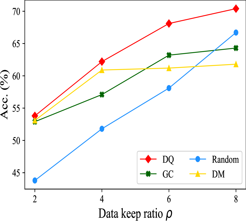
(b) Level 2

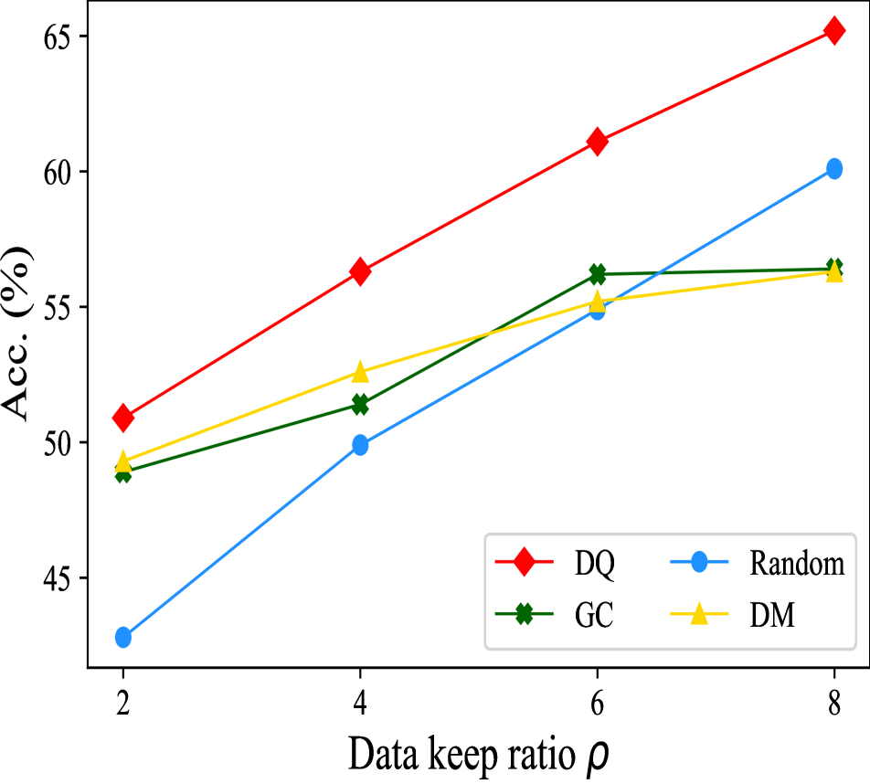
(c) Level 3

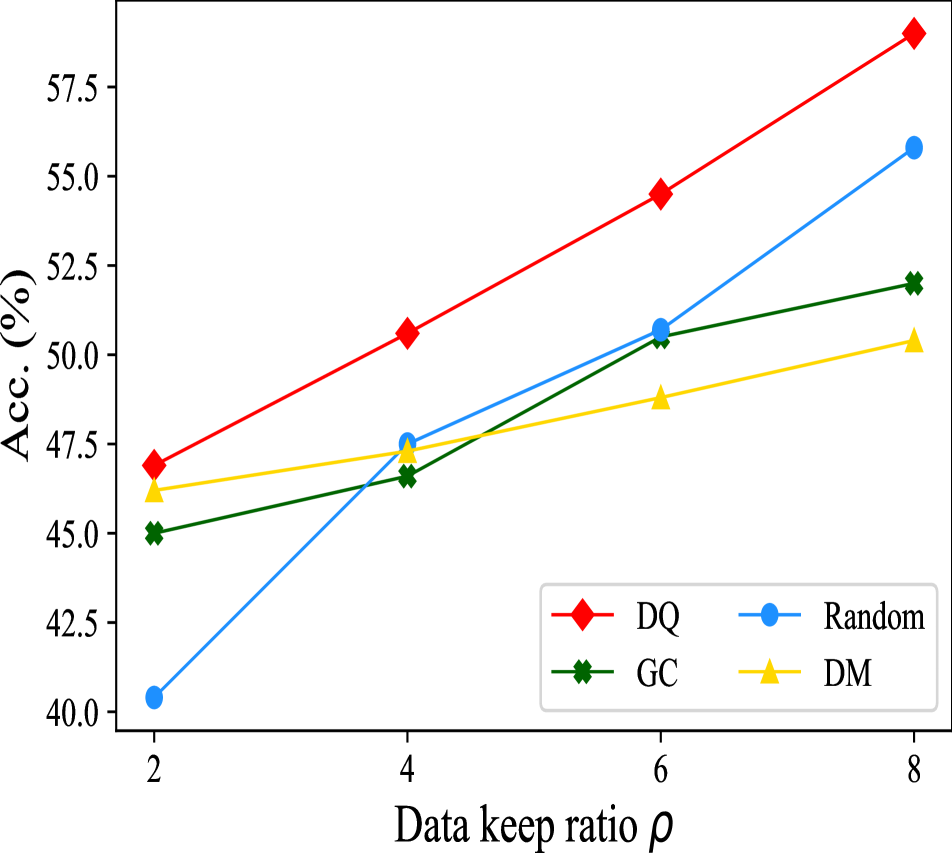
(d) Level 4

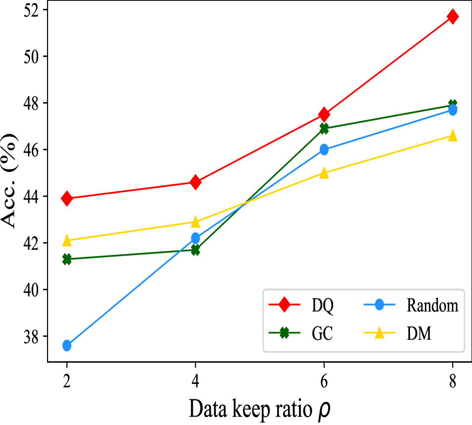
(e) Level 5

Figure 1: Comparisons of the robustness of trained models via DQ, GC and Random selection on CIFAR10-C dataset.

1.5 Differences between coreset selection and dataset quantization

Coreset VS DQ

We here give more detailed explanations on the difference between the coreset selection methods and our proposed dataset quantization. As shown in Fig. 2, the coreset selection only select one subset from the full data distribution. This practice will suffer from a selection bias, resulting in selection results with limited diversity. Besides, when the the size of the selected subset is small, it will suffer a large selection variance. Differently, dataset quantization first divides the full distribution into non-overlapping bins and then sampling from each bin uniformaly. As a result, the sampled data could maximally preserve the original data distribution. To verify this, we use GraphCut  [iyer2021submodular] as a representation of the coreset based method and 10% and 20% data from ImageNet dataset and compare the results with the data distribution sampled with dataset quantization. We use a pre-trained ResNet-18 model to extract the features of the data and then visualize the extracted data via t-SNE. The results are shown in Fig. 3. It is clearly observed that the data sampled via dataset quantization  do capture a more diverse distribution.

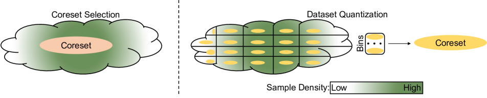
Figure 2: Differences between coreset selection methods and our dataset quantization.

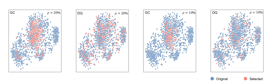
Figure 3: Visualization of the feature distributions among data selected by GraphCut and SQ.

Bin diversity of DQ

To dig deeper for the reason why DQ can better preserved the data distribution. We use the same visualization method as aforementioned for the data contained within each bin. The results are shown in Fig. 4. Each bin contains 20% of the total data in the left column and 10% data in the right column. As shown, different bins are capturing different distributions. As a results, after sampling uniformly from each bin, the combined dataset enjoys a large diversity as well as representativeness over the whole data distribution.

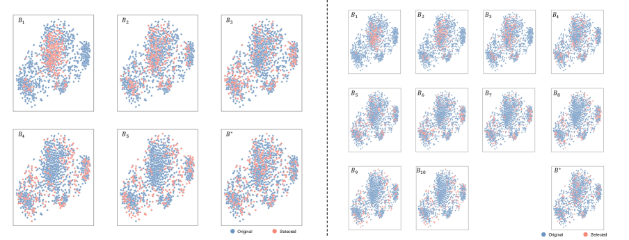
Figure 4: Visualization of the feature distributions among data selected in each bin and the final output of SQ on ImageNet dataset tench class. The bin number $N$ and the data keep ratio $\rho$ are set as (5, 20), (10, 10), respectively for the left and right column.

Cross-architecture generalization of DQ

We further present more feature distribution visualizations with different network architectures on ImageNet-1K in Fig. 5. The samples are originally selected by ResNet-18 and reconstructed with MAE. Each set contains 10% of the total data. As shown, across all architectures, the generated compact set can effectively cover the whole data distribution, presenting significant cross-architecture generalization capability.

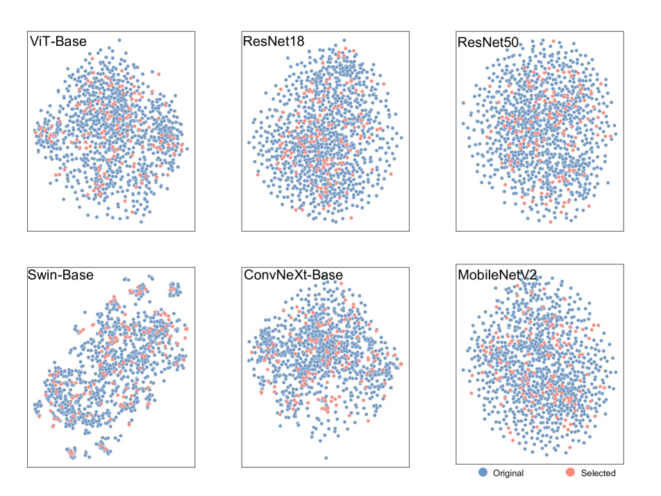
Figure 5: Cross-architecture visualiztaion of the feature distributions among the dataset generated by DQ on ViT-Base on ImageNet dataset tench class.