(a)	(b)		(c)	(d)

Figure 1. Our framework facilitate point pattern design by representing both density and correlation as a three-channel raster image (a). These images can be edited (c) in terms of their density or correlation using off-the-shelf image manipulation software. The resulting point patterns are shown before (b) and after the edits (d). Please see the accompanied supplemental material for vector graphic images.

Patternshop: Editing Point Patterns by Image Manipulation

Abstract.

Point patterns are characterized by their density and correlation. While spatial variation of density is well-understood, analysis and synthesis of spatially-varying correlation is an open challenge. No tools are available to intuitively edit such point patterns, primarily due to the lack of a compact representation for spatially varying correlation. We propose a low-dimensional perceptual embedding for point correlations. This embedding can map point patterns to common three-channel raster images, enabling manipulation with off-the-shelf image editing software. To synthesize back point patterns, we propose a novel edge-aware objective that carefully handles sharp variations in density and correlation. The resulting framework allows intuitive and backward-compatible manipulation of point patterns, such as recoloring, relighting to even texture synthesis that have not been available to 2D point pattern design before. Effectiveness of our approach is tested in several user experiments. Code is available at https://github.com/xchhuang/patternshop.

1. Introduction

Point patterns are characterized by their underlying density and correlations. Both properties can vary over space (Fig. 1), but two key challenges limit the use of such patterns: first, a reliable representation and, second, the tools to manipulate this representation.

While algorithms [Zhou et al., 2012; Öztireli and Gross, 2012] are proposed in the literature to generate point patterns with specific correlations (e.g., blue-, green-, pink-, etc. noise), designing specific correlation requires understanding of the power spectrum or Pair Correlation Function (PCF) [Heck et al., 2013] only a handful of expert users might have. Further, the space spanned by these colored noises (correlations) is also limited to a handful of noises studied in the literature [Zhou et al., 2012; Öztireli and Gross, 2012]. Addressing this, we embed point correlations in a 2D space in a perceptually optimal way. In that space, two point correlations have similar 2D coordinates if they are perceptually similar. We simply sample all realizable point correlations and perform Multidimensional scaling (MDS) on a perceptual metric, without the need for user experiments, defined on the pairs of all samples. Picking a 2D point in that space simply selects a point correlation. Moving a point changes the correlation with perceptual uniformity.

The next difficulty to adopt point patterns of spatially varying density and correlations is the lack of tools for their intuitive manipulation. Modern creative software gives unprecedented artistic freedom to change images by relighting [Pellacini, 2010], painting [Strassmann, 1986; Hertzmann et al., 2001], material manipulation [Pellacini and Lawrence, 2007; Di Renzo et al., 2014], changing canvas shape [Rott Shaham et al., 2019], completing missing parts [Bertalmio et al., 2000], as well as transferring style  [Gatys et al., 2016] or textures [Efros and Freeman, 2001; Zhou et al., 2018; Sendik and Cohen-Or, 2017]. Unfortunately, no such convenience exists when aiming to manipulate point patterns as previous approaches are specifically designed to process three-channel (RGB) raster images. Our core idea is to convert point patterns into off-the-shelf three-channel raster image. We use the $CIELAB$ color space to encode density as one-dimensional luminance (L) and two-dimensional chroma (AB) as correlation. The resulting images can the be manipulated harnessing all the power of typical raster image editing software.

While spatially-varying density is naturally mapped to single-channel images, this is more difficult for correlation. Hence, it is often assumed spatially-invariant and represented by either the power spectrum [Ulichney, 1987; Lagae and Dutre, 2008] or the PCF [Wei and Wang, 2011; Öztireli and Gross, 2012]. Some work also handles spatially-varying density or/and correlation [Chen et al., 2013; Roveri et al., 2017], but with difficulties in handling sharp variation of density and/correlation. We revisit bilateral filtering to handle sharp variation both in density and correlation.

Finally, we show how to generate detailed spatial $CIELAB$ maps of correlation and density given an input point pattern using a learning-based system, trained by density and correlation supervision on a specific class of images, e.g., human faces.

In summary, we make the following contributions:

• Two-dimensional perceptual embedding of point correlations,

• Spatially-varying representation of point pattern density and perceptually-embedded correlation as LAB raster images,

• A novel definition of edge-aware correlation applicable to hard edges in density and/or correlation,

• An optimization-based system to synthesize point patterns defined by density and embedded correlation maps according to said edge-aware definition,

• Intuitive editing of point pattern correlation and density by recoloring, painting, relighting, etc. of density and embedded correlation maps in legacy software such as Adobe Photoshop.

• A learning-based system to predicts density and embedded correlation maps from an input point pattern.

2. Previous Work

Sample correlations

Correlations among stochastic samples are widely studied in computer graphics. From halftoning [Ulichney, 1987], reconstruction [Yellott, 1983], anti-aliasing [Cook, 1986; Dippé and Wold, 1985] to Monte Carlo integration [Durand, 2011; Singh et al., 2019], correlated samples have made a noticeable impact. Recent works [Xu et al., 2020; Zhang et al., 2019] have also shown direct impact of correlated samples on training accuracy in machine learning. Among different sample correlations, blue noise [Ulichney, 1987] is the most prominent in literature. Blue noise enforces point separation and is classically used for object placement [Kopf et al., 2006; Reinert et al., 2013] and point stippling [Deussen et al., 2000; Secord, 2002; Schulz et al., 2021]. However, modern approaches do not insist on point separation in faithful stippling [Martín et al., 2017; Kim et al., 2009; Deussen and Isenberg, 2013; Rosin and Collomosse, 2012]. Different kind of colored noises (e.g., green, red) are studied in literature [Lau et al., 1999; Zhou et al., 2012] for half-toning and stippling purposes. But the space spanned by these point correlations is limited to a few bases [Öztireli and Gross, 2012]. We propose an extended space of point correlations that helps express large variety of correlations. Our framework embeds these correlations in a two-dimensional space, allowing representation of different correlations with simple two-channel color maps. This makes analysis and manipulation of correlations easier by using off-the-shelf image editing software.

Analysis

To analyze different sample correlations, various spectral [Ulichney, 1987; Lagae and Dutre, 2008] and spatial [Wei and Wang, 2011; Öztireli and Gross, 2012] tools are developed. For spectral methods, the Fourier power spectrum and it’s radially averaged version are used to analyze sample characteristics. In the spatial domain, PCF is used for analysis which evaluates pairwise distances between samples that are then binned in a 1D or a 2D histogram.

Synthesizing blue-noise correlation

Blue noise sample correlation is most commonly used in graphics. There exist various algorithms to generate blue noise sample distributions (see Yan et al. [2015]). Several optimization-based methods [Lloyd, 1982; Balzer et al., 2009; Liu et al., 2009; Schmaltz et al., 2010; Fattal, 2011; De Goes et al., 2012; Heck et al., 2013; Kailkhura et al., 2016; Qin et al., 2017], as well as tiling-based [Ostromoukhov et al., 2004; Kopf et al., 2006; Wachtel et al., 2014] and number-theoretic approaches [Ahmed et al., 2015; Ahmed et al., 2016, 2017] are developed over the past decades to generate blue noise samples.

Varying density and correlation	Varying density, constant correlation	Constant density, varying correlation
Varying density Varying correlation	Varying density Constant correlation	Constant density Varying correlation

Figure 2. Our framework allows manipulating density and correlations independently. Top row shows the point set synthesized using the density (left) and the correlation map (right) shown in the bottom row. The first column shows a point set when both density and correlation are spatially varying. Second column has constant correlation but spatially varying density. Third column point set reproduces the Siggraph logo just from spatially varying correlations.

Synthesizing other correlations

There exist methods to generate samples with different target correlations. For example, Zhou et al. [2012] and Öztireli and Gross [2012] proposed to synthesize point correlations defined from a user-defined target PCF. Wachtel et al. [2014] proposed a tile-based optimization approach that can generate points with a user-defined target power spectrum. All these methods require heavy machinery to ensure the optimization follows the target. Leimkühler et al. [2019] simplified this idea and proposed a neural network-based optimization pipeline. All these approaches, however, require the user to know how to design a realizable PCF or a power spectrum [Heck et al., 2013]. This can severely limit the usability of point correlations to only handful of expert users. Our framework lifts this limitation and allows us to simply use a two-dimensional space to define correlations. Once a user picks a 2D point —which we visualize as color of different chroma— our framework automatically finds the corresponding PCF from the embedded space and synthesizes the respective point correlations. It is also straightforward to generate spatially varying correlations using our framework by defining a range of colors as correlations. So far, only Roveri et al. [2017] have synthesized spatially varying correlations but remain limited by how well a user can design PCFs.

Image and point pattern editing

Editing software allows artists to tailor the digital content to their needs. Since color image is the easily available data representation, today’s software are specifically designed to process three-channel (RGB) images. Modern pipelines allow effects like relighting [Sun et al., 2019], recoloring, image retargeting [Rott Shaham et al., 2019], inpainting [Bertalmio et al., 2000], style transfer [Gatys et al., 2016] and texture synthesis [Efros and Freeman, 2001; Zhou et al., 2018; Sendik and Cohen-Or, 2017] to be performed directly in the three-channel RGB representation. However, most digital assets e.g., materials, color pigments, light fields, patterns, sample correlations, are best captured in high-dimensional space. This makes it hard for image-based software to facilitate editing these components. A lot of research has been devoted in the past to support editing materials [Pellacini and Lawrence, 2007; An et al., 2011; Di Renzo et al., 2014], light fields [Jarabo et al., 2014], color pigments [Sochorová and Jamriška, 2021], natural illumination [Pellacini, 2010] with workflows similar to images.

Synthesizing textures with elements [Ma et al., 2011; Reinert et al., 2013; Emilien et al., 2015; Reddy et al., 2020; Hsu et al., 2020] and patterns with different variations [Guerrero et al., 2016] using 2D graphical primitives has also been proposed. These work focus on updating point and element locations to create patterns for user-specific goals and designing graphical interface for user interactions. However, none of the previous work allows editing spatially-varying point correlations in an intuitive manner. In this work, we propose a pipeline to facilitate correlation editing using simple image operations. Instead of directly working with points, we encode their corresponding spectral or spatial statistics in a low-dimensional (3-channel) embedding. This low-dimensional latent space can then be represented as an image in order to allow artists to manipulate point pattern designs using any off-the-shelf image editing software. There exists previous work that encode point correlations [Leimkühler et al., 2019] for a single target or point pattern structures [Tu et al., 2019] using a neural network. But these representations do not disentangle the underlying density and correlation, thereby, not facilitating editing operations.

Latent and perceptual spaces

Reducing high-dimensional signals into low-dimensional ones has several benefits. Different from latent spaces in generative models which are still high-dimensional, such as for StyleGAN [Abdal et al., 2019], the application we are interested in here is a usability one, where the target space is as low as one-, two- or three- dimensional, so users can actively explore it, e.g., on a display when searching [Duncan and Humphreys, 1989]. This is common to do for color itself [Fairchild, 2013; Nguyen et al., 2015]. Ideally, the embedding into a lower dimension is done such, that distance in that space is proportional to perceived distances [Lindow et al., 2012]. This was pioneered by Pellacini et al. [2000] for BRDF, with a methodology close to ours (MDS). Other modalities, such as acoustics [Pols et al., 1969], materials [Wills et al., 2009], textures [Henzler et al., 2019] and even fabricated objects [Piovarči et al., 2018] were successfully organized in latent spaces.

3. Overview

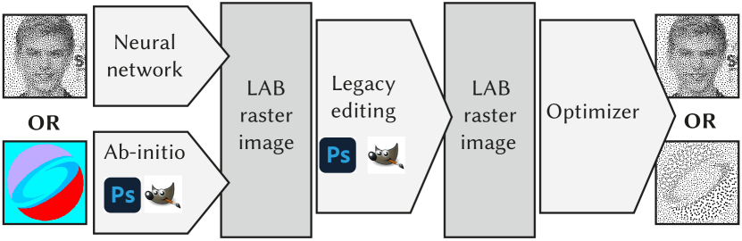
Figure 3. The workflow of Patternshop. A user can select a point pattern and run it through a NN to produce a three-channel raster image, or draw that image directly, ab-initio in a program like Adobe Photoshop or GIMP. The edited pattern can be synthesized using our optimization.

\begin{overpic}[scale={1.46},grid=false]{images/our_approach/embedding_overview_powspectra_four} \footnotesize\put(18.0,2.3){$m$ } \put(0.25,-1.0){(a) Radial power spectrum profiles} \put(24.0,-1.0){(b) Realized point sets} \put(45.0,-1.0){(c) VGG feature maps} \put(65.0,-1.0){feature vectors} \put(78.0,-1.0){Dissimilarity matrix} \put(92.0,-1.0){2D latent space} \footnotesize\put(39.2,10.0){VGG} \put(87.0,9.9){MDS} \put(63.0,-1.0){(d)} \put(76.0,-1.0){(e)} \put(90.5,-1.0){(f)} \end{overpic}

Figure 4. We illustrate the embedding from $m$ -dimensional space to a 2D space. (a) Random power spectra are generated and their corresponding realizable point patterns in (b) are synthesized using gradient descent. The point patterns are then rasterized and pass through a pre-trained VGG network [Simonyan and Zisserman, 2015] to generate (c) feature maps, which are flattened into feature vectors (d). A dissimilarity matrix (e) computed from these VGG feature vectors are used to bring $m$ -dimensional representation to a 2D space (f) using MDS (Sec. 4).

Fig. 3 shows the workflow of Patternshop: A user selects a point pattern with spatially varying density and correlation and runs this through a NN to produce a three-channel raster image. Alternatively, they can draw that image directly, ab-initio in a program like Adobe Photoshop or GIMP. This raster image can then be edited in any legacy software. Density can be manipulated by editing luminance. To change correlation, we provide a perceptual 2D space of point correlations (Fig. 5). This space is perceptually uniform, i.e., distances are proportional to human perception and covers a wide range, i.e., it contains most realizable points correlations. Figure 2 demonstrates one such example edit. A user may edit spatially varying density (Fig. 2b) or correlation (Fig. 2c) or both (Fig. 2a) using our three-channel representation. A final optimizer produces the edited point pattern.

Correlations are generally characterized by a PCF or power spectrum. A PCF encodes spatial statistics—e.g., the pairwise distances between points—distributed over an $m$ -bin histogram. Handling such an $m$ -dimensional correlation space is neither intuitive nor supported by existing creative software. To tackle this problem, in Sec. 4, we embed Pair Correlation Function (PCF) into a two-dimensional space. We optimize the distance between all pairs of latent coordinates in that space to be proportional to the perceived visual distance between their point pattern realizations.

Moreover, synthesizing such patterns requires support for edge-aware transitions for both density and correlation. In Sec. 5, we outline our formalism to handle such edge-aware density and correlations. Sec. 6 defines the optimization objective, that enables finding a point pattern to have the desired density and correlation. Sec. 7 provides details on the implementation. Sec. 8 outlines various application scenarios supported by our pipeline, followed by comparative analyses, concluding discussions and future works.

4. Latent embedding of point correlations

Overview

In order to encode the correlation of a point pattern as a 2D coordinate, we first generate a corpus of basic point patterns (each with constant correlation). Next, we extract perceptual features of these patterns. The pairwise distance between all features forms a perceptual metric. This metric is used to embed a discrete set of basis correlations into a 2D space. From this discrete mapping, we can further define a continuous mapping from any continuous correlations into a latent space as well as back from any continuous latent space coordinate to correlations. This process is a pre-computation, only executed once, and its result can be used to design many point patterns, same as one color space can be used to work with many images. We detail each step in the following:

Data generation

First, we systematically find a variety of point patterns to span a gamut of correlations $\{g_{i}\}$. We start by defining a power spectrum as a Gaussian mixture of either (randomly) one or two modes with means randomly uniform across the domain and uniform random variance of up to a quarter of the unit domain (Fig. 4a). Not all such power spectra are realizable, therefore, we run a gradient descent optimization [Leimkühler et al., 2019] to obtain realizable point patterns (Fig. 4b). We finally use the PCF of that realization $P_{i}$ as $g_{i}$. Please see Supplemental Sec. 1.1 for details.

Metric

A perceptual metric $\mathcal{D}_{i,j}$ assigns a positive scalar to every pair of stimuli $i$ and $j$ (here: point patterns) which is low only if the pair is perceived similar. As point patterns are stationary textures, their perception is characterized by the spatially aggregated statistics of their visual features [Portilla and Simoncelli, 2000]. Hence, the perceived distance between any two point patterns with visual features $\mathbf{v}_{i}$ and $\mathbf{v}_{j}$ is their $\mathcal{L}_{1}$ distance $\mathcal{D}_{i,j}=|\mathbf{v}_{i}-\mathbf{v}_{i}|_{1}$.

To compute visual feature statistics $\mathbf{v}_{i}$ for one pattern $P_{i}$, we first rasterize $P_{i}$ three times with point splats of varying Gaussian splat size of 0.015, 0.01 and 0.005 [Tu et al., 2019]. Second, each image of that triplet is converted into VGG feature activation maps [Simoncelli and Olshausen, 2001]. Next, we compute the Gram matrices [Gatys et al., 2016] for the pool_2 and pool_4 layers in each of the three images. Finally, we stack the triplet of pairs of Gram matrices into a vector $\mathbf{v}_{i}$ of size $3\times(64^{2}+128^{2})=61440$.

Figure 4 shows four example patterns leading to a $4\times 4$ dissimilarity matrix.

Dimensionality reduction

To first map the basis set of $\{P_{i}\}$ to latent 2D codes, we apply MDS (Fig. 4f). MDS assigns every pattern $P_{i}$ a latent coordinate $\mathbf{z}_{i}$ so that the joint stress of all assignments

(1) $$c_{\mathrm{Emb}}(\{\mathbf{z}_{i}\}) =\sum_{i,j}(\mathcal{D}_{i,j}-||\mathbf{z}_{i}-\mathbf{z}_{j}||)^{2}$$

is minimized across the set $\{\mathbf{z}_{i}\}$ of latent codes.

After optimizing with Eq. 1, we rotate the latent coordinates, so that blue noise is indeed distributed around a bluish color of the chroma plane and then normalize the 2D coordinates to $[0,1]^{2}$.

Encoding

Once the latent space is constructed, we can sample correlation $g$ at any continuous coordinate $\mathbf{z}$ in the latent space using the Inverse Distance Weighted (IDW) method:

(2) $$f(\mathbf{z}) =\sum_{i}g_{i}w_{i}(\mathbf{z})/\sum_{i}w_{i}(\mathbf{z})\quad\text{with}$$

(3) $$w_{i}(\mathbf{z}) =1/\max((||\mathbf{z}-\mathbf{z}_{i}||_{2})^{\phi(\mathbf{z})},10^{-10}).$$

The idea is to first compute the distance between the current location $\mathbf{z}$ and the existing locations $\mathbf{z}_{i}$ in the MDS space. The inverse of these distances, raised to a power $\phi(\mathbf{z})$, is used as the weight to interpolate the correlations $g_{i}$. $\phi\in\mathbb{R}^{2}\mapsto\mathbb{R}$ is a function that is low in areas of the latent space with a low density of examples and high for areas where MDS has embedded many exemplars. We implement $\phi$ by kernel density estimation on the distribution $\{\mathbf{z}_{i}\}$ itself with a Parzen window of size 0.01 and clamping and scaling this density linearly to the $(3,6)$-range.

Decoding

We can now also embed any correlation $\bar{g}$ , that is not in the discrete basis set $\{g_{i}\}$. Let $\bar{\mathbf{v}}$ be the visual features stats of $\bar{g}$ . We simply look up the visual-feature-nearest training exemplar and return its latent coordinate

(4) $$f^{-1}(g)=\operatorname{arg\,min}_{\mathbf{z}_{i}}||\bar{\mathbf{v}}-\mathbf{v}_{i}||_{2}.$$

\begin{overpic}[scale={1.09},grid=false]{images/mds_space} \end{overpic}

Figure 5. The left image shows the resynthesized point pattern with a continuously varying correlations in the 2D latent space $f(\mathbf{z})$. The bottom-right (black) square shows different coordinates and their color in $CIELAB$ . Point patterns with the corresponding spatially-invariant correlations for each of these coordinates are shown with respective color coding in the right halve. Blue noise can be spotted on the top-right side of the space.

Latent space visualizations

The latent space $f(\mathbf{z})$ of correlations is visualized in Fig. 5 and more visualizations can be found in Supplemental Fig. 5. Every point in $f(\mathbf{z})$ is a PCF and we use the machinery that will be defined in Sec. 6.1 to generate a point pattern that has such a spatially-varying correlation.

5. Edge-aware density and correlations

Assumptions

Input to this step is a discrete point pattern $P$ , a continuous density map $d$ and a continuous guidance map $h$ to handle spatially-varying correlations. The aim is to estimate correlation at one position so it is unaffected by points that fall onto locations on the other side of an edge. Output is a continuous spatially-varying correlation map.

Definition

We define the edge-aware radial density function as

(5) $$\hat{g}(P,d,h)(\mathbf{x},r)=\sum_{i=1}^{n}\kappa(\mathbf{x},\mathbf{x}_{i},r,d,h),$$

a mapping from location $\mathbf{x}$ , radius $r$ to density, conditioned on the point pattern $P$ with $n$ points subject to the kernel

(6) $$\kappa(\mathbf{x},\mathbf{x}_{i},r,d,h)=\frac{\hphantom{\sum_{\mathbf{y}\in\mathbb{R}^{2}}}\mathcal{S}(\mathbf{x}_{i},\mathbf{x},r,d)\cdot\mathcal{H}(\mathbf{x}_{i},\mathbf{x},h)}{\sum_{\mathbf{y}\in\mathbb{R}^{2}}\mathcal{S}(\mathbf{y},\mathbf{x},r,d)\cdot\mathcal{H}(\mathbf{y},\mathbf{x},h)},$$

that combines a spatial term $\mathcal{S}$ and a guidance term $\mathcal{H}$ , both to be explained next. Intuitively, this expression visits all discrete points $\mathbf{x}_{i}$ and soft-counts if they are in the “relevant distance” and on the “relevant side” of the edge relative to a position $\mathbf{x}$ and a radius $r$ . The $\mathbf{y}$ locations represent a dense grid used to compute the normalization term as explained next.

Spatial term

The spatial $\mathcal{S}$ -term is a Gaussian $\mathcal{N}$ with mean $r$ and standard deviation (bandwidth) $\sigma$ . It is non-zero for distances similar to $r$ and falls of with bandwidth $\sigma$ :

(7) $$\mathcal{S}(\mathbf{x}_{i},\mathbf{x},r,d)=\mathcal{N}\left(\frac{||\mathbf{x}_{i}-\mathbf{x}||_{2}}{d(\mathbf{x})};r,\sigma\right)$$

The distance between two points is scaled by the density at the query position. As suggested by Zhou et al. [2012], this assures that the same pattern at different scales, i.e., densities, indeed maps to the same correlation. Bandwidth $\sigma$ is chosen proportional to the number of points $n$ .

Guidance term

The $\mathcal{H}$ -term establishes if two points $\mathbf{x}$ and $\mathbf{x}_{i}$ in the domain are related. This is inspired by the way Photon Mapping adapts its kernels to the guide by external information such as normals [Jensen, 2001] or joint image processing makes use of guide images [Petschnigg et al., 2004]. If $\mathbf{x}$ is related to $\mathbf{x}_{i}$, $\mathbf{x}_{i}$ is used to compute correlation or density around $\mathbf{x}$, otherwise, it is not. Relation of $\mathbf{x}$ and $\mathbf{x}_{i}$ is measured as the pair similarity

(8) $$\mathcal{H}(\mathbf{x},\mathbf{x}_{i},h)=||h(\mathbf{x})^{\mathsf{T}}\cdot\Sigma\cdot h(\mathbf{x}_{i})||,$$

where $h$ is a guidance map and $\Sigma$ is the (diagonal) bandwidth matrix, controlling how guide dimensions are discriminating against each other. The guidance map can be anything with distances defined on it, but our results will use correlation itself.

Normalization

The denominator in Eq. 6 makes the kernel sum to 1 when integrated over $\mathbf{y}$ for a fixed $\mathbf{x}$ as in normalized convolutions [Knutsson and Westin, 1993]. Also, if $\kappa$ extends outside the domain for points close to the boundary, this automatically re-scales the kernel.

Example

\begin{overpic}[width=195.12767pt]{images/Kernel} \put(42.0,32.0){$\mathbf{x}$ } \end{overpic}

Figure 6. Density estimation kernel.

Fig. 6 shows this kernel in action. We show the upper left corner of the domain (white) as well as some area outside the domain (grey with stripes). Correlation is computed at the yellow point $\mathbf{x}$ . The kernel’s spatial support is the blue area. The area outside the domain (stripes) will get zero weight. Also, the grey area inside the domain which is different in the guide (due to different correlation) is ignored, controlled by the $\mathcal{H}$ -term.

Discussion

Our formulation is different from the one used by Chen et al. [2013], who warp the space to account for guide differences, as Wei and Wang [2011] did for density variation. This does not work for patterns with varying correlation: a point on an edge of a correlation should not contribute to the correlation of another point in a scaled way. Instead of scaling space, we embed points into a higher dimensional space [Chen et al., 2007; Jensen, 2001] only to perform density estimation on it.

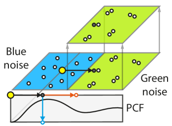
Figure 7. Bilateral.

Consider estimating the PCF at the yellow point, close to an edge between an area of blue and an area of green noise as shown on Fig. 7. The dark gray point lies on the other side of the edge. In common bilateral handling, it would contribute to a different bin (orange horizontal movement, distance in PCF space) in the formulation of Wei [2010], which is adequate for density, but not for correlation. Our approach suppresses those points (blue arrow and vertical movement, density in PCF space).

6. Synthesis and Editing

We will now derive a method to synthesize a point pattern with a desired spatially varying target density and correlation (Sec. 6.1). Users can then provide these target density and correlation as common raster images (Sec. 6.2) and edit them in legacy software (Sec. 6.3).

6.1. Synthesizing with desired correlation and density

Given Eq. 5 we can estimate $\hat{g}(P,d,h)$, the spatially-varying PCF field for a triplet of point pattern $P$ , density map $d$ and guidance map $h$ . Recall, we can also compare this spatially-varying PCF to another one, we shall call $\bar{g}$ , e.g., by spatially and radially integrating their point-wise norms. Hence, we can then optimize for a point pattern $P$ to match a given density map $d$ , a given guidance map $h$ and a given target PCF $\bar{g}$ by

(9) $$\operatorname{arg\,min}_{P}c_{\mathrm{Syn}}(P)=\int_{x}\int_{r}(\hat{g}(P,d,h)(\mathbf{x},r)-\bar{g}(\mathbf{x},r))^{2}\,\mathrm{d}\mathbf{x}\,\mathrm{d}r.$$

We use $\bar{g}$ as our guidance map $h$ to evaluate $\hat{g}$ . Note, that we do not explicitly ask the result $P$ to have a specific density. This happens implicitly: recall, that our edge-aware correlation estimate Eq. 7 will scale point-wise distances according to density before computing the PCF. Hence, the only way for the optimization to produce the target $\bar{g}$ is to scale the distances proportional to density.

In practice, we Monte Carlo-estimate this objective using $10\times 10$ jittered samples $\{\mathbf{q}_{i}\}\in[0,1]^{2}$ along the spatial dimension and $m$ regular samples $\{r_{j}\}$ along the radius dimension (ranging from $0.1$ to $2r_{\mathrm{max}}$ as detailed in Sec. 7), as in

(10) $$\hat{c}_{\mathrm{Syn}}(P)=\sum_{i=1}^{10\times 10}\sum_{j=1}^{m}(\hat{g}(P,d,\bar{g})(\mathbf{q}_{i},r_{j})-\bar{g}(\mathbf{q}_{i},r_{j}))^{2}.$$

and optimize over $P$ using ADAM [Kingma and Ba, 2014].

To have this synthesis produce a point pattern $P$ , a user now only needs to provide a spatially-varying density $d$ and correlation $\bar{g}$ .

6.2. Encoding into raster images

Users provide density $d$ , and correlation $\bar{g}$ as common discrete raster images on which we assume suitable sampling operations to be defined (e.g., bilinear interpolation) to evaluate them at continuous positions.

For density $d$ , this is trivial and common practice in the point pattern literature. For correlation, $\bar{g}$ , we use our embedding $f$ from Sec. 4 to decode the complex PCF from a latent 2D coordinate, from only two numbers per spatial location. Hence, density and correlation require only three numbers per spatial position. We pack those three number into the three image color channels. More specifically, density into the $L$ and latent correlation into the $AB$ channel of a $CIELAB$ color image, we call $F$ .

6.3. Editing point patterns as raster images

Any editing operation that is defined on a three-channel image in any legacy image manipulation software can now be applied to the point pattern feature image $F$ .

Working in $CIELAB$ color space, users have freedom to select the first-channel to edit density, the two latter channels to edit the correlations, or edit both at the same time. Since $L$ and $AB$ channels do not impact each other, $CIELAB$ color space is ideal for manipulating the density or the correlation independently as luminance and chrominance are perceptually decorrelated by-design.

While this is in a sense the optimal space to use when editing point patterns in legacy image editing software, it is not necessarily an intuitive user interface. In a fully-developed software system, on top of legacy software, a user would not be shown colors or pick colors to see, respectively, edits, correlations. Instead, they would only be presented the point pattern, and select from an image similar to Fig. 5, and all latent encoding would be hidden. We will give examples of such edits in Sec. 8. For the case of ab-initio design, no input point pattern is required and a user would freely draw correlation and density onto a blank canvas.

(a)	(b)		(c)	(d)

Figure 8. We start with a given density and correlation map (a), and perform edits directly on this three-channel raster image (c) to obtain the point pattern in (d) after resynthesis. In (c), we edit the density map ($L$ -channel) with gradients from left to right and edit correlations in the $AB$ -channel to enhance different segments of the image. No neural network is used here. Source image credit: Artmajeur user Bianchini Jr. Used with permission under Media Licence.

Input points	Network output	Our editing	Synthesized points

Figure 9. Input points (first column) generated by our synthesis and mapped to raster images (second column). An edit is performed in Adobe Photoshop (third column), and the a new point patterns is resynthesized (fourth column). In the first row, we edit the background correlation using the $AB$ channels and add some flowers on the hair using the $L$ channel. The second row shows another edit where we change the correlation in the background using the $AB$ channels. In the third row we change the correlation in the background ($AB$ channels) and add a density gradient ($L$ channel). To generate the results in the second column from the first column, we use the neural networks trained on our human faces, animal faces and churches datasets, respectively.

7. Implementation

We implement our framework mainly in PyTorch [Paszke et al., 2017]. All experiments run on a workstation with an NVIDIA GeForce RTX 2080 graphics card and an Intel(R) Core(TM) i7-9700 CPU @ 3.00GHz.

Embedding

In total, we collect 1,000 point patterns and each of them has 1,024 point samples. To perform MDS, the 2D latent coordinates $\{\mathbf{z}_{i}\}$ are initialized randomly in $[0,1]^{2}$. The MDS optimization Eq. 1 runs in batches of size $20$, using the ADAM optimizer [Kingma and Ba, 2014] with a learning rate of $0.005$ for $1,000$ iterations.

If latent coordinates are quantized to 8 bit, there is only $256^{2}$ many different possible correlations $\{g_{i}\}$. We pre-compute these and store them in a $256\times 256\times m$ look-up table $\mathtt{lut}$ w.r.t. each latent 2D coordinate to be used from here on.

Input points	Output synthesized points	Input points	Output synthesized points

Figure 10. Our NN maps the input point pattern to a density and correlation map. To obtain different point pattern editing effects, we apply different advanced filters to the output density map. From left, the second column shows the relighting effect using the method by ClipDrop [2023]. Fourth column shows the change in the facial expression and the eyes direction performed using a neural filter from Adobe Photoshop.

Edge-aware PCF estimator

To compute the pair similarity between two guide values in $h$ , the bandwidth matrix $\Sigma$ is set to be $0.005$-diagonal. We use $m=20$ bins to estimate the PCF. The binning is performed over the distance range from 0.1 to 2 $r_{\mathrm{max}}$, where $r_{\mathrm{max}}=2\sqrt{\frac{1}{2\sqrt{3}n}}$. The point count $n$ is chosen as the product between a constant and the total inverse intensity in the $L$ -channel of the given feature image $F$ , such that an image with dark pixels has more points. To compute local PCF for each pixel in $F$ , we consider only the $k$-nearest neighbor points, and not all points, where $k=50$ and $\sigma=0.26$.

With each PCF, $g_{i}$ we also pre-compute and store $\lambda_{i}$, the best Learning Rate (LR) (see Supplemental Sec. 1.2 for a definition) as we found different spectra to require different LRs. During synthesis, we find the LR for every point, by sampling the correlation map at that point position and using the LR of the manifold-nearest exemplar of that correlation.

Synthesis

The initial points when minimizing Eq. 9 are randomly sampled in $[0,1]^{2}$ proportional to the density map $d$ and the optimization runs for $5,000$ iterations. We note that the denominator in Eq. 5 is a sum over many points which could be costly to evaluate, but as it does not depend on the point pattern $P$ itself, it can be pre-computed before optimizing Eq. 9. We use C++ and Pybind11 to accelerate this computation and the whole initialization stage takes around $5$ seconds.

To faithfully match the intensity of point stipples with the corresponding density map [Spicker et al., 2017], we also optimize for dot sizes as a post processing step.

Editing

We use Adobe Photoshop 2022 for editing which has native $CIELAB$ support. We devised two simple interfaces scripted into Adobe Photoshop 2022, one for interactive visualization of colors and point correlations and the other for editing and synthesis.

\begin{overpic}[scale={2.55},grid=false]{images/texture_synthesis/texture_synthesis_comparison_tu_lowres} \put(-2.0,16.0){\rotatebox{90.0}{Input points}} \put(-2.0,1.0){\rotatebox{90.0}{Network output}} \put(19.0,28.7){After editing operation} \put(50.0,28.7){Our edit-aware output} \put(80.0,28.7){\cite[citet]{\@@bibref{Authors Phrase1YearPhrase2}{tu2019pointpattern}{\@@citephrase{[}}{\@@citephrase{]}}}} \end{overpic}

Figure 11. Starting from an input pattern of tree cover density (left, top), we use a network specialized on geomatic data to estimate correlation and density (left, bottom). We can then apply existing image operations, such as Adobe Photoshop’s “Content-Aware Fill” (second column) to achieve “Point Pattern Expansion” (third column), which compares favorably to direct optimization of points to match the inputs’ VGG-based Gram matrices, deep correlation matrices and histograms [Tu et al., 2019] (last column).

	Input	Ours (Gram)	Ours (PCF 1K)	Öztireli and Gross [2012] (PCF 8K)
PCF	​​	​​	​​	​​
PCF	​​	​​	​​	​​

Figure 12. For an input point pattern, we query its nearest neighbor in the latent space. Using Gram matrices (middle-left) the nearest neighbor quality is closer to the input than using PCFs (middle-right). The inset images alongside PCFs show the latent space coordinates. The correlation space from Öztireli and Gross [2012] uses 8K PCFs but is still not diverse enough to provide good nearest neighbor for the input. Our latent space has only 1000 base point patterns. We also perform a user study on this as detailed in Sec. 8.6.

8. Results

In this section, we demonstrate our design choices and compare our pipeline with existing methods through some application scenarios. We also perform a user study to evaluate the effectiveness and usability of our framework. More results can be found in the accompanied supplemental material.

8.1. Ab-initio point pattern design

We demonstrate examples of point pattern edits in Fig. 1 and Fig. 8. We start with a given density and correlation map (1st and 3rd columns). We choose blue noise for the correlation map to start with and start editing both the density ($L$ -channel) and the correlation ($AB$ -channel). For Fig. 1, we add density gradient transition on the background and add a simple leaf by editing the density channel. We also assign different correlations to different segments like the butterfly, leaf and background. For Fig. 8, the correlation edits are done in the $AB$ channel of the Picasso image to assign different correlations to different image segments, e.g., background, face, cap and the shirt. We also add a gradient density in the background from left to right by editing the $L$ -channel of the image.

We show more results in Supplemental Fig. 4 to demonstrate that our framework provides a straightforward way to edit spatially-varying point correlations by picking correlations from our correlation space (Fig. 5), instead of by designing PCFs or power spectra.

8.2. Neural network-aided point pattern design

Besides manually drawing correlation and density, we propose a second alternative: a NN, based on pix2pix [Isola et al., 2017], which automatically produces density and correlation maps from legacy point patterns. We curated paired synthetic datasets for class-specific training from three categories, including human faces from CelebA by Lee et al. [2020], animal faces from Choi et al. [2020] and churches from Yu et al. [2015]. As the NN maps point patterns to raster images, training data synthesis proceeds in reverse: For each of the three-channel raster image, the gray-scale image of each original image is directly used as the $L$ -channel. We generate the correlation map ($AB$ -channel) by assigning them random chroma i.e., latent correlation coordinates. Next, our synthesis from Sec. 6.1 is used to instantiate a corresponding point pattern. Finally the patterns is rasterized, as pix2pix works with raster images. For further data generation, network architecture and training details, please see Supplemental Sec. 1.4. We also perform an ablation study on the network architecture and training in Supplemental Fig. 6.

This pipeline enables freely changing local density or correlation in point patterns of different categories as seen in  Fig. 9. As shown in Fig. 10, this also allows advanced filtering such as relighting or facial expression changes on point patterns. In Supplemental Fig. 7, we show additional results where the input point patterns, generated by other image stippling methods [Zhou et al., 2012] [Salaün et al., 2022], can be edited using our framework.

8.3. Point pattern expansion

Here we train our network on density from the Tree Cover Density [Büttner and Kosztra, 2017] dataset in combination with random spatially-varying correlation maps using anisotropic Gaussian kernel with varying kernel size and rotation as detailed in Supplemental Sec. 1.3. Similar works can be found in Kapp et al. [2020], Tu et al. [2019] and Huang et al. [2022] for sketch-based or example-based point distribution synthesis.

Figure 11 illustrates one such representative example of point-based texture synthesis using our method. Our network reconstructs the density and correlation map that captures the gradient change of correlation and spatially-varying density. By using the content-aware filling tool in Adobe Photoshop, we can perform texture expansion (second column) based on the network output. More specifically, we first expand the canvas size of the map, select the unfilled region, and use content-aware filling to automatically fill the expanded background. We also compare our method with a state-of-the-art point pattern synthesis method from Tu et al. [2019] which takes an exemplar point pattern as input and uses VGG-19 [Simonyan and Zisserman, 2015] features for optimization.

8.4. Realizability

We construct the manifold Fig. 5 from exemplars that are realizable, but an interpolation of realizable PCFs is not guaranteed to be realizable. We test if realizability still holds in practice as follows. For each PCF $g(\mathbf{z}_{i})$, we generate a point set instance using our method and compute the resulting PCF $g^{\prime}(\mathbf{z}_{i})$. We then compute $A=\mathbb{E}_{i}[(|g^{\prime}(\mathbf{z}_{i})-g(\mathbf{z}_{i})|)]$, the average error between PCF and realized PCF and $B=\max_{ij}(|g(\mathbf{z}_{j})-g(\mathbf{z}_{i})|)$ the maximum difference between any two PCFs. The relative error A/B is $3\times 10^{-5}$, indicating that the realization error is five order of magnitude smaller than the PCF signal itself.

8.5. Comparisons

Comparisons with Öztireli and Gross [2012]

To the best of our knowledge, Öztireli and Gross [2012] is the most relevant related work which studies the space of point correlations using PCFs. However, we observe that PCFs are not the best way to characterize the perceptual differences between different point correlations. In Fig. 12, we show that the Gram matrices (our input proximity to MDS) better encode the perceptual similarity between neighboring point correlations.

Roveri et al. [2017]	Ours

Figure 13. We compare the synthesis quality of our optimization against Roveri et al. [2017]. To run Roveri et al. method (left), we use the stored PCFs within each pixel of $F$ . The zoom-ins in the bottom two rows show that Roveri et al. cannot handle well the sharp transitions in the correlations.

Comparisons with Roveri et al. [2017]

Figure 13 shows an example of synthesizing point patterns using our synthesis method and the synthesis method proposed by Roveri et al. [2017]. To the best of our knowledge, Roveri et al. [2017] is the only competitor that supports point pattern synthesis from spatially-varying density and correlation. We demonstrate that their method may synthesize point patterns with artifacts around the sharp transitions between two correlations (bottom-right and top-left of the logo). Our method, by taking the bilateral term into account, can handle sharp transition between correlations more accurately.

This relation can be further quantified as follows: Let $P$ be a point pattern, ${\bar{P}}$ be an edited version of that and $g(P)$, respectively, $g({\bar{P}})$ be their correlations. Now, first, let $g_{\mathrm{PCA}}({\bar{P}})$ be the correlations of ${\bar{P}}$ , projected into the space spanned by the PCA of the correlations in and only in $P$ , and, second, $g_{\mathrm{Ours}}({\bar{P}})$ be the correlations of ${\bar{P}}$ , projection into our palette (Fig. 5). The error of those projections is $e_{\mathrm{PCA}}=|g_{\mathrm{PCA}}({\bar{P}})-g({\bar{P}})|$ and $e_{\mathrm{Ours}}=|g_{\mathrm{Ours}}({\bar{P}})-g({\bar{P}})|$ , respectively. We evaluate these error values for different figures. Fig. 1 shows 96$\times$ improvement, Fig. 8 shows 130$\times$ improvement and the three rows in Fig. 9 shows 471$\times$, 461$\times$ and 59$\times$ improvement using our approach ($e_{\mathrm{Ours}}$ vs. $e_{\mathrm{PCA}}$). This indicates that our latent space can preserve one to two order of magnitudes more edit details than Roveri et al. [2017] approach which restricts itself to the input exemplar.

8.6. User study

We performed a set of user experiments to verify i) the perceptual uniformity of our embedding ii) the ability of users to navigate in that space iii) the usefulness of the resulting user interface.

Embedding user experiment

34 subjects (S) were shown a self-timed sequence of 9 four-tuples of point patterns with constant density and correlation in a horizontal arrangement (Fig. 12). The leftmost pattern was a reference. The three other patterns were nearest neighbors to the reference in a set of: i) our basis patterns using our perceptual metric, ii) our basis patterns using PCF metric, and iii) patterns from the PCF space suggest by Öztireli and Gross [2012] using PCF metric. Ss were instructed to rate the similarity of each of the three leftmost patterns to the reference on a scale from 1 to 5 using radio buttons.

The mean preferences, across the 10 trials, were a favorable 3.59, 2.52 and 2.55 which is significant ($p<.001$, two-sided $t$-test) for ours against both other methods. A per-pattern breakdown is seen in Fig. 14. This indicates our metric is perceptually more similar to user responses than two other published ones. Figure 12 shows two examples where the nearest-neighbor of the query point pattern is perceptually different using different metrics. The PCF of two point patterns can be similar even when they are perceptually different.

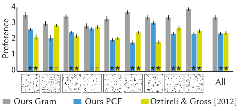
Figure 14. Results of the embedding user experiment. Errors bars are standard errors of the mean. A black or gray star is significance against our method at the $p=.001$ or $.005$-level.

Latent space as points (see Fig. 5)	Chroma ($AB$ -channel)

Figure 15. Results of the navigation user experiment. Users are shown the latent space visualized as spatially-varying points (Fig. 5) on the left and as spatially-varying chroma on the right. The large dots represent the locations of our selected $8$ reference point patterns. The small dots are the locations that the users chose as perceptually similar point patterns wrt. the reference.

Navigation user experiment

In this experiment, $N=9$ Ss were shown, $8$ reference point correlations and, second, the palette of all correlations covered by our perceptual embedding (Fig. 5). Ss were asked to pick coordinates in the second image by clicking locations in the embedding, so that the corresponding point correlations of the picked coordinates perceptually match the reference correlations.

The users’ locations were off by 14.9 % of the embedding space diagonal. We would not be aware of published methods for intuitive correlation design to compare this number to. Instead, we have compared to the mistakes users make when picking colors using the LAB color picker in Adobe Photoshop. Another $N=9$ Ss, independent to the ones shown the palette of correlations, made an average mistake of 21.3% in that case. We conclude, that our embedding of pattern correlation into the chroma plane is significantly more intuitive ($p<0.2$, $t$ test) than picking colors. Fig. 15 shows the points users clicked (small dots), relative to the true points (large dots).

Input	Target	User 1	User 2	User 3

Figure 16. User edits from the usefulness experiment. We show that users can use our system to design point patterns (first row) by editing $L$ -channel and $AB$ -channel (second row) to match the target one from an initialized input.

Usefulness experiment

Ss were asked to reproduce a target stippling with spatially varying correlation and density by means of Adobe Photoshop that was enhanced to handle point correlation as LAB space using our customized interface. Ss were shown the point patterns of our perceptual latent space, and asked to edit the density and correlation separately to reproduce the reference from an initialized LAB image. After each editing, generating the point pattern incurred a delay of one minute. Note that we intentionally reduce the number of iterations to optimize the point patterns from user edits to offer faster feedback in around a minute with around 10,000 points. Details on this experiment are found in Supplemental Sec. 2.4. There is no objective metric to measure the result quality, so we report three user-produced point patterns in Fig. 16. The whole process takes 15 minutes on average for all three users, as they usually require multiple trials on picking the correlations and our synthesis method does not run interactively.

8.7. Performance

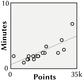
Figure 17. Timing.

We summarize the run-time statistics of our synthesis method w.r.t. the number of synthesized points in Fig. 17. Editing time is not reported as it can be biased by the editing skills of the users.

9. Conclusion and Future Work

We propose a novel framework to facilitate point pattern design, by introducing a perceptual correlation space embedded in a two-channel image using a dimensionality reduction method (MDS). This allows users to design or manipulate density and correlation by simply editing a raster image using any off-the-shelf image editing software. Once edited, the new features can be resynthesized to the desired point pattern using our optimization (Sec. 6.1). To better handle sharp transitions in density and correlation during synthesis, we formulate a novel edge-aware PCF (Sec. 5) estimator. The resulting framework allows wide range of manipulations using simple image editing tools that were not available to point patterns before. Users can design novel spatially varying point correlations and densities without any expert knowledge on PCF or power spectra or can use a NN to get correlation and density for a specific class, such as faces.

Limitations

The latent space spanned by the bases point correlations in Fig. 5 is by no means perfect. Synthesizing point patterns with smooth transitions from two extreme locations in the latent space may result in some unwanted artifacts. Our synthesis method takes minutes to synthesize points which is far from interactive rate that is more friendly to artists and users.

Future work

A neural network with such latent space is a promising direction where the correlations within the geomatic data can be predicted and edited according to user-defined conditions (environment, pollution, global warming, etc). Our approach happens to rasterize points, which ideally is to be replaced by directly operating on points Qi et al. [2017]; Hermosilla et al. [2018].

The editing operations can also be improved by proper artistic guidance or by interactive designing tools that intuitively manipulate the desired density and correlations for desired goals. Extending our pipeline for visualization purposes is another fascinating future direction. Another interesting future direction is to extend the current pipeline to multi-class and multi-featured point patterns, which appear in real-world patterns. Designing a latent pattern space that spans a larger gamut of correlations (also anisotropic and regular ones) present in nature (e.g., sea shells, tree, stars, galaxy distributions) is a challenging future problem to tackle. There is an exciting line of future works that can be built upon our framework. Many applications like material appearance, haptic rendering, smart-city design, re-forestation, planet colonization can benefit from our framework.

References

- [1]
- Abdal et al. [2019] Rameen Abdal, Yipeng Qin, and Peter Wonka. 2019. Image2stylegan: How to embed images into the stylegan latent space?. In ICCV. 4432–4441.
- Ahmed et al. [2017] Abdalla GM Ahmed, Jianwei Guo, Dong-Ming Yan, Jean-Yves Franceschia, Xiaopeng Zhang, and Oliver Deussen. 2017. A simple push-pull algorithm for blue-noise sampling. IEEE Trans. Vis and Comp. Graph. 23, 12 (2017).
- Ahmed et al. [2015] Abdalla GM Ahmed, Hui Huang, and Oliver Deussen. 2015. AA patterns for point sets with controlled spectral properties. ACM Trans. Graph. 34, 6 (2015).
- Ahmed et al. [2016] Abdalla GM Ahmed, Hélène Perrier, David Coeurjolly, Victor Ostromoukhov, Jianwei Guo, Dong-Ming Yan, Hui Huang, and Oliver Deussen. 2016. Low-discrepancy blue noise sampling. ACM Trans. Graph. 35, 6 (2016).
- An et al. [2011] Xiaobo An, Xin Tong, Jonathan D. Denning, and Fabio Pellacini. 2011. AppWarp: Retargeting Measured Materials by Appearance-Space Warping. ACM Trans. Graph. 30, 6 (2011), 1–10.
- Balzer et al. [2009] Michael Balzer, Thomas Schlömer, and Oliver Deussen. 2009. Capacity-constrained point distributions: a variant of Lloyd’s method. ACM Trans. Graph. 28, 3 (2009).
- Bertalmio et al. [2000] Marcelo Bertalmio, Guillermo Sapiro, Vincent Caselles, and Coloma Ballester. 2000. Image Inpainting. In Proc. SIGGRAPH. 417–424.
- Büttner and Kosztra [2017] György Büttner and Barbara Kosztra. 2017. CLC2018 Technical Guidelines. Technical Report. European Environment Agency.
- Chen et al. [2013] Jiating Chen, Xiaoyin Ge, Li-Yi Wei, Bin Wang, Yusu Wang, Huamin Wang, Yun Fei, Kang-Lai Qian, Jun-Hai Yong, and Wenping Wang. 2013. Bilateral blue noise sampling. ACM Trans. Graph. 32, 6 (2013), 1–11.
- Chen et al. [2007] Jiawen Chen, Sylvain Paris, and Frédo Durand. 2007. Real-time edge-aware image processing with the bilateral grid. ACM Trans. Graph. 26, 3 (2007), 103–113.
- Choi et al. [2020] Yunjey Choi, Youngjung Uh, Jaejun Yoo, and Jung-Woo Ha. 2020. Stargan v2: Diverse image synthesis for multiple domains. In Proceedings of the IEEE/CVF conference on computer vision and pattern recognition. 8188–8197.
- ClipDrop [2023] ClipDrop. 2023. Relight API. https://clipdrop.co/relight
- Cook [1986] Robert L Cook. 1986. Stochastic sampling in computer graphics. ACM Trans. Graph. 5, 1 (1986).
- De Goes et al. [2012] Fernando De Goes, Katherine Breeden, Victor Ostromoukhov, and Mathieu Desbrun. 2012. Blue noise through optimal transport. ACM Trans. Graph. 31, 6 (2012).
- Deussen et al. [2000] Oliver Deussen, Stefan Hiller, Cornelius Van Overveld, and Thomas Strothotte. 2000. Floating points: A method for computing stipple drawings. In Comp. Graph. Forum, Vol. 19. 41–50.
- Deussen and Isenberg [2013] Oliver Deussen and Tobias Isenberg. 2013. Halftoning and Stippling. In Image and Video-Based Artistic Stylisation, Paul Rosin and John Collomosse (Eds.). Springer London, 45–61.
- Di Renzo et al. [2014] Francesco Di Renzo, Claudio Calabrese, and Fabio Pellacini. 2014. AppIm: Linear Spaces for Image-Based Appearance Editing. ACM Trans. Graph. 33, 6 (2014).
- Dippé and Wold [1985] Mark A. Z. Dippé and Erling Henry Wold. 1985. Antialiasing through Stochastic Sampling. In SIGGRAPH. 69–78.
- Duncan and Humphreys [1989] John Duncan and Glyn W Humphreys. 1989. Visual search and stimulus similarity. Psychological review 96, 3 (1989), 433.
- Durand [2011] Frédo Durand. 2011. A frequency analysis of Monte-Carlo and other numerical integration schemes. Technical Report TR-2011-052. MIT CSAIL.
- Efros and Freeman [2001] Alexei A. Efros and William T. Freeman. 2001. Image Quilting for Texture Synthesis and Transfer. In SIGGRAPH. 341–346.
- Emilien et al. [2015] Arnaud Emilien, Ulysse Vimont, Marie-Paule Cani, Pierre Poulin, and Bedrich Benes. 2015. Worldbrush: Interactive example-based synthesis of procedural virtual worlds. ACM Trans. Graph. 34, 4 (2015), 1–11.
- Fairchild [2013] Mark D Fairchild. 2013. Color appearance models. John Wiley & Sons.
- Fattal [2011] Raanan Fattal. 2011. Blue-noise point sampling using kernel density model. ACM Trans. Graph. 30, 4 (2011).
- Gatys et al. [2016] Leon A. Gatys, Alexander S. Ecker, and Matthias Bethge. 2016. Image Style Transfer Using Convolutional Neural Networks. In CVPR. 2414–2423.
- Guerrero et al. [2016] Paul Guerrero, Gilbert Bernstein, Wilmot Li, and Niloy J. Mitra. 2016. PATEX: Exploring Pattern Variations. ACM Trans. Graph. 35, 4 (2016).
- Heck et al. [2013] Daniel Heck, Thomas Schlömer, and Oliver Deussen. 2013. Blue noise sampling with controlled aliasing. ACM Trans. Graph. (Proc. SIGGRAPH) 32, 3 (2013).
- Henzler et al. [2019] Philipp Henzler, Niloy J Mitra, , and Tobias Ritschel. 2019. Learning a Neural 3D Texture Space from 2D Exemplars. In CVPR.
- Hermosilla et al. [2018] Pedro Hermosilla, Tobias Ritschel, Pere-Pau Vázquez, Àlvar Vinacua, and Timo Ropinski. 2018. Monte Carlo Convolution for Learning on Non-uniformly Sampled Point Clouds. ACM Trans. Graph (Proc. SIGGRAPH Asia) 37, 5 (2018).
- Hertzmann et al. [2001] Aaron Hertzmann, Charles E Jacobs, Nuria Oliver, Brian CNOurless, and David H Salesin. 2001. Image analogies. In SIGGRAPH. 327–340.
- Hsu et al. [2020] Chen-Yuan Hsu, Li-Yi Wei, Lihua You, and Jian Jun Zhang. 2020. Autocomplete element fields. In Proc. CHI. 1–13.
- Huang et al. [2022] Xingchang Huang, Pooran Memari, Hans-Peter Seidel, and Gurprit Singh. 2022. Point-Pattern Synthesis using Gabor and Random Filters. In Comp. Graph. Forum, Vol. 41. 169–179.
- Isola et al. [2017] Phillip Isola, Jun-Yan Zhu, Tinghui Zhou, and Alexei A Efros. 2017. Image-to-Image Translation with Conditional Adversarial Networks. CVPR (2017).
- Jarabo et al. [2014] Adrian Jarabo, Belen Masia, Adrien Bousseau, Fabio Pellacini, and Diego Gutierrez. 2014. How Do People Edit Light Fields? ACM Trans. Graph. 33, 4 (2014).
- Jensen [2001] Henrik Wann Jensen. 2001. Realistic image synthesis using photon mapping. AK Peters/crc Press.
- Kailkhura et al. [2016] Bhavya Kailkhura, Jayaraman J Thiagarajan, Peer-Timo Bremer, and Pramod K Varshney. 2016. Stair blue noise sampling. ACM Trans. Graph. 35, 6 (2016).
- Kapp et al. [2020] Konrad Kapp, James Gain, Eric Guérin, Eric Galin, and Adrien Peytavie. 2020. Data-driven authoring of large-scale ecosystems. ACM Trans. Graph. 39, 6 (2020), 1–14.
- Kim et al. [2009] Sung Ye Kim, Ross Maciejewski, Tobias Isenberg, William M. Andrews, Wei Chen, Mario Costa Sousa, and David S. Ebert. 2009. Stippling by Example. In Proc. NPAR. 41–50.
- Kingma and Ba [2014] Diederik P Kingma and Jimmy Ba. 2014. Adam: A method for stochastic optimization. arXiv preprint arXiv:1412.6980 (2014).
- Knutsson and Westin [1993] Hans Knutsson and C-F Westin. 1993. Normalized and differential convolution. In CVPR. 515–523.
- Kopf et al. [2006] Johannes Kopf, Daniel Cohen-Or, Oliver Deussen, and Dani Lischinski. 2006. Recursive Wang tiles for real-time blue noise. ACM Trans. Graph. (Proc. SIGGRAPH) 25, 3 (2006).
- Lagae and Dutre [2008] Ares Lagae and Philip Dutre. 2008. A Comparison of Methods for Generating Poisson Disk Distributions. Comp. Graph. Forum 27, 1 (2008).
- Lau et al. [1999] Daniel L. Lau, Gonzalo R. Arce, and Neal C. Gallagher. 1999. Digital halftoning by means of green-noise masks. J OSA 16, 7 (1999), 1575–1586.
- Lee et al. [2020] Cheng-Han Lee, Ziwei Liu, Lingyun Wu, and Ping Luo. 2020. MaskGAN: Towards Diverse and Interactive Facial Image Manipulation. In CVPR.
- Leimkühler et al. [2019] Thomas Leimkühler, Gurprit Singh, Karol Myszkowski, Hans-Peter Seidel, and Tobias Ritschel. 2019. Deep Point Correlation Design. ACM Trans. Graph. 38, 6 (2019).
- Lindow et al. [2012] Norbert Lindow, Daniel Baum, and Hans-Christian Hege. 2012. Perceptually linear parameter variations. In Comp. Graph. Forum, Vol. 31. 535–544.
- Liu et al. [2009] Yang Liu, Wenping Wang, Bruno Lévy, Feng Sun, Dong-Ming Yan, Lin Lu, and Chenglei Yang. 2009. On centroidal Voronoi tessellation – energy smoothness and fast computation. ACM Trans. Graph. 28, 4 (2009).
- Lloyd [1982] Stuart Lloyd. 1982. Least squares quantization in PCM. IEEE Trans Inform. Theory 28, 2 (1982).
- Ma et al. [2011] Chongyang Ma, Li-Yi Wei, and Xin Tong. 2011. Discrete Element Textures. ACM Trans. Graph. 30, 4 (2011).
- Martín et al. [2017] Domingo Martín, Germán Arroyo, Alejandro Rodríguez, and Tobias Isenberg. 2017. A survey of digital stippling. Computers & Graphics 67 (2017), 24–44.
- Nguyen et al. [2015] Chuong H Nguyen, Tobias Ritschel, and Hans-Peter Seidel. 2015. Data-driven color manifolds. ACM Trans. Graph. 34, 2 (2015), 1–9.
- Ostromoukhov et al. [2004] Victor Ostromoukhov, Charles Donohue, and Pierre-Marc Jodoin. 2004. Fast hierarchical importance sampling with blue noise properties. ACM Trans. Graph. 23, 3 (2004).
- Öztireli and Gross [2012] A Cengiz Öztireli and Markus Gross. 2012. Analysis and synthesis of point distributions based on pair correlation. ACM Trans. Graph. 31, 6 (2012).
- Paszke et al. [2017] Adam Paszke, Sam Gross, Soumith Chintala, Gregory Chanan, Edward Yang, Zachary DeVito, Zeming Lin, Alban Desmaison, Luca Antiga, and Adam Lerer. 2017. Automatic differentiation in pytorch. (2017).
- Pellacini [2010] Fabio Pellacini. 2010. envyLight: An Interface for Editing Natural Illumination. ACM Trans. Graph. (SIGGRAPH) (2010).
- Pellacini et al. [2000] Fabio Pellacini, James A Ferwerda, and Donald P Greenberg. 2000. Toward a psychophysically-based light reflection model for image synthesis. In SIGGRAPH. 55–64.
- Pellacini and Lawrence [2007] Fabio Pellacini and Jason Lawrence. 2007. AppWand: Editing Measured Materials Using Appearance-Driven Optimization. ACM Trans. Graph. 26, 3 (2007), 54–64.
- Petschnigg et al. [2004] Georg Petschnigg, Richard Szeliski, Maneesh Agrawala, Michael Cohen, Hugues Hoppe, and Kentaro Toyama. 2004. Digital photography with flash and no-flash image pairs. ACM Trans. Graph. 23, 3 (2004), 664–672.
- Piovarči et al. [2018] Michal Piovarči, David I.W. Levin, Danny Kaufman, and Piotr Didyk. 2018. Perception-Aware Modeling and Fabrication of Digital Drawing Tools. ACM Trans. Graph. (SIGGRAPH) 37, 4 (2018).
- Pols et al. [1969] Louis CW Pols, LJ Th Van der Kamp, and Reinier Plomp. 1969. Perceptual and physical space of vowel sounds. J ASA 46, 2B (1969), 458–467.
- Portilla and Simoncelli [2000] Javier Portilla and Eero P Simoncelli. 2000. A parametric texture model based on joint statistics of complex wavelet coefficients. Int. J Computer Vision 40 (2000), 49–70.
- Qi et al. [2017] Charles R Qi, Hao Su, Kaichun Mo, and Leonidas J Guibas. 2017. Pointnet: Deep learning on point sets for 3D classification and segmentation. CVPR (2017).
- Qin et al. [2017] Hongxing Qin, Yi Chen, Jinlong He, and Baoquan Chen. 2017. Wasserstein Blue Noise Sampling. ACM Trans. Graph. 36, 5 (2017).
- Reddy et al. [2020] Pradyumna Reddy, Paul Guerrero, Matt Fisher, Wilmot Li, and Niloy J. Mitra. 2020. Discovering Pattern Structure Using Differentiable Compositing. ACM Trans. Graph. 39, 6 (2020).
- Reinert et al. [2013] Bernhard Reinert, Tobias Ritschel, and Hans-Peter Seidel. 2013. Interactive By-Example Design of Artistic Packing Layouts. ACM Trans. Graph. 32, 6 (2013).
- Rosin and Collomosse [2012] Paul Rosin and John Collomosse. 2012. Image and Video-Based Artistic Stylisation. Springer Publishing Company, Incorporated.
- Rott Shaham et al. [2019] Tamar Rott Shaham, Tali Dekel, and Tomer Michaeli. 2019. SinGAN: Learning a Generative Model from a Single Natural Image. In ICCV.
- Roveri et al. [2017] Riccardo Roveri, A. Cengiz Öztireli, and Markus Gross. 2017. General Point Sampling with Adaptive Density and Correlations. Comp. Graph. Forum 36, 2 (2017), 107–117.
- Salaün et al. [2022] Corentin Salaün, Iliyan Georgiev, Hans-Peter Seidel, and Gurprit Singh. 2022. Scalable Multi-Class Sampling via Filtered Sliced Optimal Transport. ACM Trans. Graph. (SIGGRAPH) 41, 6 (2022).
- Schmaltz et al. [2010] Christian Schmaltz, Pascal Gwosdek, Andres Bruhn, and Joachim Weickert. 2010. Electrostatic Halftoning. Comp. Graph. Forum (2010).
- Schulz et al. [2021] Christoph Schulz, Kin Chung Kwan, Michael Becher, Daniel Baumgartner, Guido Reina, Oliver Deussen, and Daniel Weiskopf. 2021. Multi-Class Inverted Stippling. ACM Trans. Graph. 40, 6 (2021).
- Secord [2002] Adrian Secord. 2002. Weighted Voronoi stippling. In Proc. NPAR.
- Sendik and Cohen-Or [2017] Omry Sendik and Daniel Cohen-Or. 2017. Deep Correlations for Texture Synthesis. ACM Trans. Graph. 36, 5 (2017).
- Simoncelli and Olshausen [2001] Eero P Simoncelli and Bruno A Olshausen. 2001. Natural image statistics and neural representation. Ann. Review Neuroscience 24, 1 (2001).
- Simonyan and Zisserman [2015] Karen Simonyan and Andrew Zisserman. 2015. Very Deep Convolutional Networks for Large-Scale Image Recognition. In Proc. ICLR, Yoshua Bengio and Yann LeCun (Eds.).
- Singh et al. [2019] Gurprit Singh, Cengiz Oztireli, Abdalla G.M. Ahmed, David Coeurjolly, Kartic Subr, Oliver Deussen, Victor Ostromoukhov, Ravi Ramamoorthi, and Wojciech Jarosz. 2019. Analysis of Sample Correlations for Monte Carlo Rendering. Comp. Graph Form. (Proc. EGSR) 38, 2 (2019).
- Sochorová and Jamriška [2021] Šárka Sochorová and Ondřej Jamriška. 2021. Practical pigment mixing for digital painting. ACM Trans. Graph. 40, 6 (2021), 1–11.
- Spicker et al. [2017] Marc Spicker, Franz Hahn, Thomas Lindemeier, Dietmar Saupe, and Oliver Deussen. 2017. Quantifying Visual Abstraction Quality for Stipple Drawings. In Proc. NPAR.
- Strassmann [1986] Steve Strassmann. 1986. Hairy brushes. SIGGRAPH 20, 4 (1986), 225–232.
- Sun et al. [2019] Tiancheng Sun, Jonathan T. Barron, Yun-Ta Tsai, Zexiang Xu, Xueming Yu, Graham Fyffe, Christoph Rhemann, Jay Busch, Paul Debevec, and Ravi Ramamoorthi. 2019. Single Image Portrait Relighting. ACM Trans. Graph. 38, 4 (2019).
- Tu et al. [2019] Peihan Tu, Dani Lischinski, and Hui Huang. 2019. Point Pattern Synthesis via Irregular Convolution. Comp. Graph. Forum 38 (2019).
- Ulichney [1987] Robert Ulichney. 1987. Digital Halftoning. MIT Press.
- Wachtel et al. [2014] Florent Wachtel, Adrien Pilleboue, David Coeurjolly, Katherine Breeden, Gurprit Singh, Gaël Cathelin, Fernando De Goes, Mathieu Desbrun, and Victor Ostromoukhov. 2014. Fast tile-based adaptive sampling with user-specified Fourier spectra. ACM Trans. Graph. 33, 4 (2014).
- Wei [2010] Li-Yi Wei. 2010. Multi-class blue noise sampling. ACM Trans. Graph. 29, 4 (2010).
- Wei and Wang [2011] Li-Yi Wei and Rui Wang. 2011. Differential domain analysis for non-uniform sampling. ACM Trans. Graph. 30, 4 (2011).
- Wills et al. [2009] Josh Wills, Sameer Agarwal, David Kriegman, and Serge Belongie. 2009. Toward a perceptual space for gloss. ACM Trans. Graph. 28, 4 (2009), 1–15.
- Xu et al. [2020] Yifan Xu, Tianqi Fan, Yi Yuan, and Gurprit Singh. 2020. Ladybird: Quasi-Monte Carlo Sampling for Deep Implicit Field Based 3D Reconstruction with Symmetry. ECCV (2020), 248–263.
- Yan et al. [2015] Dong-Ming Yan, Jian-Wei Guo, Bin Wang, Xiao-Peng Zhang, and Peter Wonka. 2015. A survey of blue-noise sampling and its applications. Journal of Comp. Sci. and Tech. 30, 3 (2015).
- Yellott [1983] John I Yellott. 1983. Spectral consequences of photoreceptor sampling in the rhesus retina. Science 221, 4608 (1983).
- Yu et al. [2015] Fisher Yu, Ari Seff, Yinda Zhang, Shuran Song, Thomas Funkhouser, and Jianxiong Xiao. 2015. Lsun: Construction of a large-scale image dataset using deep learning with humans in the loop. arXiv preprint arXiv:1506.03365 (2015).
- Zhang et al. [2019] Cheng Zhang, Cengiz Öztireli, Stephan Mandt, and Giampiero Salvi. 2019. Active Mini-Batch Sampling Using Repulsive Point Processes. AAAI.
- Zhou et al. [2012] Yahan Zhou, Haibin Huang, Li-Yi Wei, and Rui Wang. 2012. Point sampling with general noise spectrum. ACM Trans. Graph. 31, 4 (2012).
- Zhou et al. [2018] Yang Zhou, Zhen Zhu, Xiang Bai, Dani Lischinski, Daniel Cohen-Or, and Hui Huang. 2018. Non-Stationary Texture Synthesis by Adversarial Expansion. ACM Trans. Graph. 37, 4 (2018).