QD-BEV : Quantization-aware View-guided Distillation for Multi-view
3D Object Detection

Abstract

Multi-view 3D detection based on BEV (bird-eye-view) has recently achieved significant improvements. However, the huge memory consumption of state-of-the-art models makes it hard to deploy them on vehicles, and the non-trivial latency will affect the real-time perception of streaming applications. Despite the wide application of quantization to lighten models, we show in our paper that directly applying quantization in BEV tasks will 1) make the training unstable, and 2) lead to intolerable performance degradation. To solve these issues, our method QD-BEV enables a novel view-guided distillation (VGD) objective, which can stabilize the quantization-aware training (QAT) while enhancing the model performance by leveraging both image features and BEV features. Our experiments show that QD-BEV achieves similar or even better accuracy than previous methods with significant efficiency gains. On the nuScenes datasets, the 4-bit weight and 6-bit activation quantized QD-BEV-Tiny model achieves 37.2% NDS with only 15.8 MB model size, outperforming BevFormer-Tiny by 1.8% with an 8$\times$ model compression. On the Small and Base variants, QD-BEV models also perform superbly and achieve 47.9% NDS (28.2 MB) and 50.9% NDS (32.9 MB), respectively.

  * Equal contribution : zhang_yifan@smail.nju.edu.cn, zhendong@berkeley.edu † Corresponding authors : ldu@nju.edu.cn, shanghang@pku.edu.cn

1 Introduction

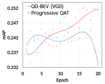
(a) mAP curve.

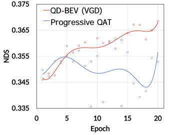
(b) NDS curve.

Figure 1: Training curves of QD-BEV (with VGD) versus progressive QAT on W4A6 quantization of BEVFormer-Tiny. Note that standard QAT works even worse compared to progressive QAT and it falls out of the targeted accuracy range in the figures.

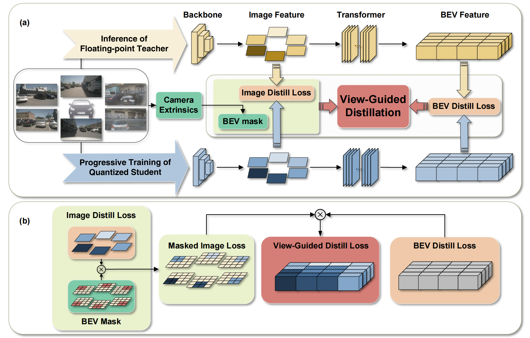
Figure 2: Illustration of QD-BEV. (a) In our pipeline, multi-camera images are input into the floating-point teacher network and the quantized student network in order to compute the KL divergence in an element-wise manner. The KL divergence is used as distillation loss in the image feature and the BEV feature, respectively. Then we conduct view-guided distillation using the BEV mask obtained from the external parameters of the camera. Please refer to Sec.3.1 for more details. (b) The lower flow chart shows the computation process of the view-guided distillation loss. Specific details are in Sec. 3.3.

Given its potential in enabling autopilot, multi-view 3D detection based on BEV (bird-eye-view) has become an important research direction for autonomous driving. Based on input sensors, previous work can be divided into LiDAR-based methods [18, 47] and camera-only methods [23, 38, 14, 13, 24, 25]. Compared to the LiDAR-based methods, camera-only methods have the merits of lower deployment cost, closer to human eyes, and easier access to visual information in the driving environment. However, even if using the camera-only methods, the computational and memory costs of running state-of-the-art BEV models are still formidable, making it difficult to deploy them onto vehicles. For example, BEVFormer-Base has a 540 ms inference latency (corresponds to 1.85 fps) on one NVIDIA V100 GPU, which is infeasible for real-time applications that generally require 30 fps. Since a non-trivial latency will harm the streaming perception, it is particularly crucial to explore and devise lightweight models for camera-only 3D object detection based on BEV.

Quantization [16, 11, 42, 10] can reduce the bitwidth used to represent weights and activations in deep neural networks, which can greatly save the model size and computational costs while improving the speed of model reasoning. However, directly applying quantization would lead to significant performance degradation. Compared to image classification and 2D object detection tasks where the standard quantization methods shine, multi-camera 3D detection tasks are much more complicated and difficult due to the existence of multiple views and information from multiple dimensions (for example, the temporal information and spatial information used in BEVFormer [23]). Consequently, the structure of BEV networks tends to become more complex, with a deeper convolutional neural network backbone to extract image information from multiple views, and with transformers to encode and decode the features of the BEV domain. The presence of different neural architectures, multiple objectives, and knowledge from different modalities greatly challenges the standard quantization methods, decreasing their stability and accuracy, and even making the whole training process diverge. In Figure 1, we show the training curves when applying W4A6 quantization on a BEVFormer-Tiny model. As can be seen, the performance of quantization-aware training (QAT) fluctuates significantly in different epochs, while the performance of our proposed method QD-BEV shows a stable rising trend. We perform more experiments to validate the effectiveness of QD-BEV in Sec 5.

To solve the problems of standard QAT, in this work, we first conduct systematic experiments and analyses on quantizing BEV networks. Then we devise a quantization-aware view-guided distillation method (referred to as QD-BEV) that can decently solve the stability issue while improving the final performance of compact BEV models. Our proposed view-guided distillation (VGD) can better leverage information from both the image and the BEV domains for multi-view 3D object detection. This can significantly outperform previous distillation methods that cannot jointly handle the different types of losses in BEV networks. Specifically, as shown in Figure 2, we first take the FP (floating-point) model as the teacher model and the quantized model as the student model, then we calculate the KL divergence on the image feature and the BEV feature, respectively. Finally, we leverage the mapping relationship and realize VGD by organically combining the image feature and the BEV feature through the camera’s external parameters. Note that in QD-BEV, neither additional training data nor larger powerful teacher networks are used to tune the accuracy, but QD-BEV models are still able to outperform previous baselines while having significantly smaller model sizes and computational requirements. Our contributions are as follows:

• We conduct systematic experiments on quantizing BEV models, unveiling major issues hampering standard quantization-aware training methods on BEV.

• We specially design view-guided distillation (VGD) for BEV models, which jointly leverages both image domain and BEV domain information. VGD boosts the final performance while solving the stability issue of standard QAT.

• Our W4A6 quantized QD-BEV-Tiny has 37.2% NDS with only 15.8 MB model size, which outperforms the 8$\times$ larger BevFormer-Tiny model by 1.8%.

2 Related Works

2.1 Camera-only 3D object detection

In camera-only 3D object detection tasks, many excellent methods have emerged based on BEV (bird-eye-view). Previous works, LSS [31] and BEVDet [14], project image features to the BEV space in a bottom-up manner. Based on DETR [5] and Deformable DETR [48], DETR3D [38] extends the 2D object detection to the 3D space through the architecture of Backbone + FPN + Decoder. In addition, PETR [24] introduces 3D position coding based on DETR3D [38]. In BEVFormer [23], the authors use dense BEV queries to exchange information in the BEV space with the multi-view image space. More stable BEV features are obtained by extracting temporal and spatial information through the transformer structure with temporal self-attention and spacial cross-attention. Based on the temporal interaction in BEVFormer, further improvements have been made in recent works, PETRv2 [25] and BEVDet4D [13]. Besides the aforementioned works, BEVDepth [21] and BEVstereo [20] are two state-of-the-art approaches for monocular depth estimation and stereo vision in the bird-eye-view (BEV) domain, respectively, which leverage the unique characteristics of BEV representations to achieve high accuracy and efficiency.

2.2 Quantization

To reduce the model size, quantization [45, 36, 15, 26] uses low bitwidth to represent weights and activations in neural networks. With the use of low-precision matrix multiplication or convolution, quantization can also make the inference process faster and more efficient. Given a pretrained model, directly performing quantization without any fine-tuning is referred to as post-training quantization (PTQ) [4, 29, 37, 17]. Despite the merits, PTQ with low bitwidth still results in significant accuracy degradation. As such, Quantization-aware training (QAT) is proposed to train the model to better adapt to quantization. QAT methods [9, 7, 40] are more costly compared to PTQ, but can potentially obtain higher accuracy. Furthermore, in the cases with ultra-low quantization bitwidth (for example, 4-bit), even QAT cannot close the accuracy gap. A promising direction to solve this is to use mixed-precision quantization [46, 36, 39], where some sensitive layers are kept at higher precision to recover the accuracy. Though effective, the support for mixed-precision quantization on general-purpose machines (CPUs and GPUs) is currently immature and may lead to extra latency overhead.

Although standard quantization methods have shown great results on convolutional neural networks, recent works [27, 44] mention that it may suffer in other neural architectures such as transformers. The presence of both convolutional blocks and transformers in BEV networks makes them challenging to the traditional quantization methods.

2.3 Distillation

Model distillation [12, 28, 22, 32, 1] generally uses a large model as the teacher to train a compact student model. Instead of using class labels during the training of the student model, the key idea is to leverage the soft probabilities produced by the teacher to guide the student’s training. Previous methods of distillation explore different knowledge sources (for example, [12, 22, 30] use logits, aka the soft probabilities). The choices of teacher models are also studied, where [41, 34] use multiple teacher models, while [8, 43] apply self-distillation without an extra teacher model. Other previous efforts apply distillation with different settings on different applications. Regarding BEV networks, previous work [6] tries to teach LiDAR information to camera-based networks through distillation, but the additional requirement for LiDAR data makes it infeasible in our pure camera-based setting. Besides, the existence of different types of losses in BEV networks makes standard distillation methods invalid. An arbitrary or sub-optimal combination of knowledge sources would also make the training unstable, perform badly, or even diverge.

3 Method

3.1 Overview of QD-BEV pipeline

This work aims to improve the efficiency of state-of-the-art BEV models. Starting with the widely used BEVFormer [23], we apply a progressive quantization-aware training procedure in a stage-by-stage manner (details are introduced in  Sec. 3.2). We further boost its stability and performance through a novel view-guided distillation process, which is highlighted in Figure 2, where we use a floating-point teacher model to facilitate the learning of our quantized QD-BEV student model. Specifically, the input multi-camera image is entered into the teacher and the student, respectively, and then the Image Backbone and Image Neck parts of the network are used to extract the multi-camera image feature. After the transformer part of the network, the BEV features are extracted, and the two parts of the teacher model and the student model are used to calculate image distill loss and BEV distill loss, respectively. The two distillation losses are then fused through the external parameters of the camera to achieve our unique view-guided distillation mechanism. We provide a detailed formulation of the view-guided distillation process in Sec. 3.3.

3.2 Quantization-aware training

In symmetric linear quantization, the quantizer maps weights and activations into integers with a scale factor $S$. Uniformly quantizing to k bit can be expressed as:

$$\begin{split}\textit{S}=\frac{2|r_{\max}|}{2^{k}-1},\ \textit{q}=\textit{round}\left(\frac{r}{S}\right)\end{split}$$ (1)

where $r$ is the floating-point number being quantized, $|r_{\max}|$ is the largest absolute value in $r$, and $q$ is the quantized integer. In this work, we conduct systematic experiments to analyze the performance of quantization on BEV networks. For PTQ, we apply the above quantization directly to the pre-trained models during the inference stage. For QAT, we utilize the straight-through estimator (STE) [2] to define the forward and backward processes for the above quantization operations, and then we train the model to better adapt to quantization. As previously mentioned in Sec. 1 and Sec. 2, considering that standard QAT may lead to divergence due to the characteristics of BEV models, we apply a stage-wise progressive QAT where we gradually reduce the weight precision in four stages (backbone, neck, encoder, and decoder) based on the design of BEVFormer [23]. The performance of this progressive QAT is illustrated in Figure 3. And we compare the effectiveness of the progressive QAT with standard QAT in Sec. 4.2.2.

3.3 View-guided distillation

Compared to traditional single-domain distillation methods, our approach exploits the complementary nature of both BEV and image domains, which provides different perspectives and capture different aspects of the scene. The BEV domain offers a top-down view, enabling accurate perception and recognition of the surrounding environment, such as the structure of the road, the location of vehicles, and lane markings. On the other hand, the image domain provides more realistic visual information, capturing rich scene details and color information. In the following sections, we present details of VGD: the computation of the image feature distillation in Sec. 3.3.1, the BEV feature distillation in Sec. 3.3.2, and the view-guided distillation combining the previous two distillation losses in Sec. 3.3.3.

3.3.1 Image feature distillation

Given a pair of aligned teacher and student models, We first compute element-wise distillation loss on image features. We extract the image neck output as the image features to be distilled. To improve the smoothness of the distillation loss, we follow previous attempts [33] to use a KL divergence-based distillation loss. Specifically, we consider the flattened image features of the student and the teacher model as logits, which we convert into probability distribution via a softmax function with temperature $\phi_{\tau}$, as defined in Eq. 2.

$${\phi_{\tau}(x_{i})}=\frac{e^{x_{i}/\tau}}{\sum_{j}e^{x_{j}/\tau}}$$ (2)

Then we calculate the KL divergence of each camera’s output separately to obtain the image feature distillation loss, as in Eq. 3.

$$\begin{split}{\mathcal{L}_{img}}=\frac{\tau^{2}}{{B}\cdot{W}\cdot{H}\cdot{C}}\times\mathcal{D}_{KL}\left(\phi_{\tau}(F^{T}_{img}),\phi_{\tau}(F^{S}_{img})\right)\end{split}$$ (3)

where B stands for the batch size, W, H, C mean the width, height, and number of channels of the image features, respectively. $F^{T}_{img}$ and $F^{S}_{img}$ denote the image features of the teacher model and the student model.

3.3.2 BEV feature distillation

We first convert the BEV features of the student and teacher into probability distributions, following the same procedure as for image features. Then we compute the KL divergence for each point on the BEV features, as shown in Eq. 4.

$$\begin{split}{\mathcal{L}_{bev}}=\frac{\tau^{2}}{{B}\cdot{C}}\times{\rm\mathcal{D}_{KL}}\left(\phi_{\tau}(F^{T}_{bev}),\phi_{\tau}(F^{S}_{bev})\right)\end{split}$$ (4)

where B stands for the batch size, C means the number of channels of BEV features. $F^{T}_{bev}$ and $F^{S}_{bev}$ denote the BEV features of the teacher model and student model, respectively. We will get a loss with the shape of $[H_{bev}\times W_{bev},1]$.

3.3.3 View-guided distillation objective

In the first two sections, we obtained the loss of each camera on the image feature and the corresponding loss of each point on the BEV feature. On the nuScenes dataset, the camera external parameters are known, so we can obtain the distribution range of each camera corresponding to the BEV feature. Then we generate the BEV mask of views $M_{bev}$ that can be applied to the image feature, which is the same as defined in BEVFormer [23]. $M_{bev}$ is a tensor with four dimensions: number of cameras, batch size, BEV size $(H_{bev}\times W_{bev})$, and 3D Height, with binary values in each element. By calculating the average along the last dimension (3D Height), we can flatten the BEV mask $M_{bev}$ on the 2d plane with the BEV size $(H_{bev}\times W_{bev})$. Then the ${\mathcal{L}_{img}}$ calculated for each camera can be extended to the corresponding loss for each point on the BEV feature, which we refer to as ${\widehat{\mathcal{L}}_{img}}$:

$$\begin{split}{\widehat{\mathcal{L}}_{img}}={\mathcal{L}_{img}}\odot M_{bev}\end{split}$$ (5)

where $\odot$ denotes the hadamard product.

Finally, we use ${\widehat{\mathcal{L}}_{img}}$ to get the view-guided distillation objective in Eq. 6:

$$\begin{split}\mathcal{L}_{vgd}={\sum_{i=1}^{N\cdot H\cdot W}}{\widehat{\mathcal{L}}_{img}}\odot{\mathcal{L}_{bev}}\end{split}$$ (6)

The overall process of view-guided distillation is shown in Algorithm 1.

Algorithm 1 Progressive Quantization-Aware VGD

Training data;

Pre-trained FP weights for teacher model $T_{fp}$;

Student model $S$;

Numbers of epochs for each phase $N_{1}$, … , $N_{4}$; $P_{2}$;

Quantization bit for weight and activation $B_{w};B_{a}$

Trained low-bit student model $S_{q}$

Phase 1: Progressive Quantization-Aware Training

Init $S_{0}$ with $T_{fp}$; Divide model into 4 $Parts$: $\{Backbone,Neck,Encoder,Decoder\}$;

for $i,module$ in $Parts$ do

     $module$ = quantize ($module$; $B_{w}$, $B_{a}$)

     Init $S_{i}$ with $S_{i-1}$

     for Epoch = $N_{i-1}$ ,…, $N_{i}$ do

         Update $S_{q_{i}}$ by minimizing QAT loss      

Phase 2: View-Guided Distillation

Init ${S}$ with $S_{4}$

for  Epoch = 1, … , $P_{2}$ do

     Update $S$ by minimizing QAT loss and $\mathcal{L}_{vgd}$ in Eq. 6

4 Experiments

In this section, we first elaborate on the experimental settings, then we evaluate both PTQ and QAT methods on the BEV networks. Based on the analysis of these results, we propose QD-BEV to overcome shortcomings in standard PTQ and QAT, and we dedicatedly compare our results with previous works under different settings and constraints.

4.1 Experimental settings

4.1.1 Dataset

We evaluated our proposed method on a challenging 3D detection task using the nuScenes dataset [3], which is a large-scale public dataset for autopilot developed by the team at Motional (formerly nuTonomy). This dataset contains 1000 manually selected 20-second driving scenarios collected in Boston and Singapore, with 750 scenarios for training, 100 for validation, and 150 for testing. The images in the dataset were captured from 6 cameras with known internal and external parameters.

Table 1: Results with PTQ separately applied on each part in BEVFormer.

Quantized Module				BEVFormer-Tiny		BEVFormer-Small		BEVFormer-Base
Backbone	Neck	Encoder	Decoder	mAP↑	NDS↑	mAP↑	NDS↑	mAP↑	NDS↑
✕	✕	✕	✕	0.252	0.354	0.370	0.479	0.416	0.517
✔	✕	✕	✕	0.212	0.310	0.288	0.417	0.309	0.440
✕	✔	✕	✕	0.252	0.353	0.370	0.478	0.416	0.516
✕	✕	✔	✕	0.181	0.295	0.298	0.421	0.160	0.303
✕	✕	✕	✔	0.251	0.353	0.369	0.477	0.416	0.517
✔	✔	✔	✔	0.145	0.246	0.228	0.369	0.075	0.224

4.1.2 Evaluation metrics

The main measurement indicators on the nuScenes 3D test dataset are the mean Average Precision (mAP), and the unique evaluation index nuScenes detection score (NDS). NDS is a comprehensive evaluation index containing many aspects of information. The other indicators are mean Average Translation Error (mATE), mean Average Scale Error (mASE), mean Average Orientation Error (mAOE), mean Average Velocity Error (mAVE) and mean Average Attribute Error (mAAE). To evaluate the efficiency of the BEV networks, we use model size and BOPS as the metrics. Model size is the memory required to store a specific network, which is determined by the total amount of parameters in the model as well as the quantization bitwidth to store those parameters. BOPS measures the total Bit Operations of one network inference [35]. It is a common metric for evaluating the computation of quantized neural networks. For a model with $L$ layers, defining $b_{w_{i}}$ and $b_{a_{i}}$ to be the bitwidth used for weights and activations of the $i$-th layer, then we have:

$$\begin{split}\textit{BOPS}=\sum\nolimits_{i=1}^{L}b_{w_{i}}b_{a_{i}}\textit{MAC}_{i}\end{split}$$ (7)

where MAC_i is the total Multiply-Accumulate operations for computing the $i$-th layer. To better demonstrate the advantages of our QD-BEV model over the floating-point model, we introduce sAP [19] (streaming average precision) as one of the evaluation metrics for our model performance. sAP is a dynamic metric that will be updated as new data arrive, making it ideal for evaluating models in real-time scenarios.

4.1.3 Baselines & Implementation Details

We mainly compare with floating-point baseline models proposed by BEVFormer [23] with different input image resolutions (specifically, BEVFormer-Tiny, BEVFormer-Small, and BEVFormer-Base). For quantization baselines, we apply the previous PTQ method DFQ [29] as well as QAT method PACT [7] and HAWQv3 [40] to quantize BEVFormer models and compare with QD-BEV.

For floating-point models, we use the open-sourced repository of BEVFormer with two different backbones: ResNet50 and ResNet101-DCN. We use symmetrical linear quantization in a channel-wise manner for weights, and layer-wise quantization for activations, which are the standard settings for previous quantization methods. Since there is little related work in our settings for reference, we make our training adopt the same scheme as the original training strategy of BEVFormer, which is to train 24 epochs in each step, and to use optimizer of AdamW, a starting lr as 2e-4, a linear warmup of 500 iters, and cosine annealing.

Table 2: PTQ results with different quantization bitwidth.

W-bit/A-bit	Model	NDS↑	NDS Drop	mAP↑
32/32	Tiny	0.354	-	0.252
	Small	0.479	-	0.370
	Base	0.517	-	0.416
8/8	Tiny	0.351	0.8%	0.248
	Small	0.477	0.4%	0.366
	Base	0.487	5.8%	0.384
6/6	Tiny	0.312	11.9%	0.203
	Small	0.430	10.2%	0.306
	Base	0.402	22.2%	0.262
4/6	Tiny	0.246	30.5%	0.146
	Small	0.369	23.0%	0.228
	Base	0.226	56.3%	0.076
4/4	Tiny	0.034	90.4%	0.001
	Small	0.034	92.9%	0.001
	Base	0.023	95.6%	0.000

Table 3: Comparsion between progressive and standard QAT with W4A6. Please refer to Table 2 for baseline FP accuracy (W32A32).

Method	Model	NDS↑	NDS Drop	mAP↑
Standard QAT	Tiny	0.326	7.9%	0.216
	Small	0.421	12.1%	0.303
	base	0.224	56.7%	0.071
Progressive QAT	Tiny	0.348	1.7%	0.234
	Small	0.467	2.5%	0.356
	base	0.485	6.2%	0.376

4.2 Analysis on BEV Quantization

Table 4: QD-BEV results compared to previous methods or baselines.

Input Size	Model	Model Size(MB)	BOPS(Tera)	NDS↑	mAP↑	mATE↓	mASE↓	mAOE↓	mAVE↓	mAAE↓
450$\times$800	BEVFormer-T[23]	126.8	62.33	0.354	0.253	0.899	0.294	0.655	0.657	0.216
	BEVFormer-T-DFQ[29]	31.7	3.90	0.340	0.236	0.949	0.296	0.651	0.671	0.217
	BEVFormer-T-HAWQv3[40]	15.9	1.46	0.348	0.234	0.949	0.304	0.568	0.661	0.209
	BEVFormer-T-PACT[7]	15.9	1.46	0.347	0.234	0.919	0.289	0.604	0.671	0.216
	QD-BEV-T (Ours)	15.9	1.46	0.372	0.255	0.882	0.321	0.543	0.599	0.214
720$\times$1280	BEVFormer-S[23]	225.6	236.13	0.479	0.370	0.722	0.279	0.407	0.438	0.220
	BEVFormer-S-DFQ[29]	56.4	14.76	0.467	0.356	0.751	0.283	0.405	0.451	0.222
	BEVFormer-S-HAWQv3[40]	28.2	5.53	0.467	0.356	0.751	0.287	0.419	0.449	0.208
	BEVFormer-S-PACT[7]	28.2	5.53	0.461	0.351	0.750	0.275	0.422	0.507	0.196
	QD-BEV-S (Ours)	28.2	5.53	0.479	0.374	0.716	0.290	0.389	0.474	0.210
900$\times$1600	BEVFormer-B[23]	262.9	667.39	0.517	0.416	0.672	0.273	0.370	0.393	0.197
	BEVFormer-B-DFQ[29]	65.7	41.71	0.486	0.384	0.771	0.274	0.378	0.427	0.206
	BEVFormer-B-HAWQv3[40]	32.9	15.64	0.485	0.376	0.727	0.288	0.381	0.434	0.202
	BEVFormer-B-PACT[7]	32.9	15.64	0.480	0.374	0.735	0.291	0.392	0.458	0.201
	QD-BEV-B (Ours)	32.9	15.64	0.509	0.406	0.691	0.285	0.360	0.410	0.190

Table 5: QD-BEV results on BEVDepth[21] and PETR[24].

W	A	Model	mAP↑	NDS↑
32	32	BEVDepth-T[21]	0.330	0.435
8	8	BEVDepth-T-DFQ[29]	0.281	0.377
4	6	BEVDepth-T-HAWQ[40]	0.136	0.206
4	6	BEVDepth-T-PACT[7]	0.270	0.362
4	6	QD-BEVDepth-T (Ours)	0.301	0.394
32	32	PETR-r50dcn[24]	0.317	0.366
8	8	PETR-r50dcn-DFQ[29]	0.290	0.343
4	6	PETR-r50dcn-HAWQ[40]	0.162	0.216
4	6	PETR-r50dcn-PACT[7]	0.268	0.320
4	6	QD-PETR-r50dcn (Ours)	0.288	0.334

4.2.1 PTQ results

We first analyze the sensitivity of different modules to quantization in Table 1. It can be seen that the backbone and the encoder parts of the network are more sensitive, while quantization of the neck and the decoder parts only brings a slight disturbance to the accuracy. We want to note that, based on the sensitivity analysis, it is possible to apply mixed-precision quantization to better preserve the sensitive modules, but we leave this as future work since it is beyond the scope of this paper.

We then analyze the influence of different quantization bitwidth on the final performance. In Table 2, directly applying PTQ with less than 8-bit precision will lead to a significant accuracy drop, especially when quantized to W4A4 the results become pure noise with around 0 mAP. As can be observed from Table 2, performing QAT is necessary in order to preserve the accuracy while achieving ultra-low bit quantization.

4.2.2 QAT results

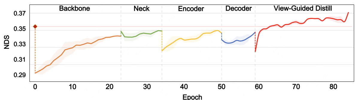
Figure 3: The training process of QD-BEV. Progressive QAT with 4 stages is performed in the first 60 epochs, then the view-guided distillation is conducted together with QAT to steadily enhance the performance. The pink line in the figure represents the baseline NDS. Note that swapping VGD with pure QAT or other distillation methods (for example, CWD [33]) will lead to undesirable results, as we show in the last 20 epochs in this figure, compared with Figure 1 and Figure 5.

To address the severe accuracy degradation of PTQ, we apply QAT to better adapt the models towards 4-bit quantization. In all our experiments, the standard QAT method which directly quantizes the whole network to the target bitwidth will lead to unstable QAT processes, causing gradient explosion or a rapid decrease in accuracy in large models (for example, the W4A6 BEVFormer-Base has only 0.07 mAP). Based on this observation, we hypothesize that the quantization perturbation introduced in standard QAT is too large to be recovered. As such, we apply progressive QAT to constrain the quantization perturbation along the training process. A comparison of the performance between progressive QAT and standard QAT with the same number of training epochs is presented in Table 3. We can see that progressive QAT consistently outperforms standard QAT by a large margin (up to 5% mAP) in BEVFormer-Tiny and BEVFormer-Small, and achieves an even larger performance gain on BEVFormer-Base. To better validate our analyses, we plot the training curve of progressive QAT as the first 60 epochs in Figure 3, where W4A6 quantization is conducted on BEVFormer-Tiny. We separate the progressive QAT into 4 stages and iteratively quantize a new module in each stage. As can be seen, there is an NDS drop at beginning of each stage, corresponding to the quantization perturbation introduced by quantizing each new module.

Despite the merits of progressive QAT, we want to note that it still suffers from unstable training and performance degradation. As illustrated in Figure 1 which corresponds to the last 20 epochs in Figure 3, progressive QAT keeps going up and down after reaching a plateau, while training curves of VGD show a rising trend with much better stability.

4.3 Main Results of QD-BEV

In order to obtain better accuracy and stability, we apply view-guided distillation with the floating-point model as the teacher and the quantized model as the student. The effect of VGD on W4A6 quantization of BEVFormer-Tiny is shown in Figure 3. Note that we separate VGD from progressive QAT in the first 60 epochs for a clearer comparison and illustration, and VGD is actually a plug-and-play function that can always be jointly applied with QAT, as we do in the last 20 epochs. Benefiting from knowledge in both the image domain and the BEV domain, QD-BEV networks are able to fully recover the quantization degradation, and even outperform the floating-point baselines. As shown in Table 4, the NDS and mAP of the model outperform previous floating-point baselines as well as quantized networks. Since there are no existing results for compact BEV networks, we implement standard quantization methods DFQ [29], HAWQv3 [40] and PACT [7] on BEVFormer as a comparison. We apply W8A8 quantization for DFQ (DFQ is a PTQ method, lower bitwidth will lead to intolerable accuracy degradation) and W4A6 for QAT methods and QD-BEV models. As a comparison, QD-BEV can achieve 0.509 NDS with only 32.9 MB model size, which is similar to the size of BEVFormer-T-DFQ (0.340 NDS) and much smaller than BEVFormer-Tiny (126.8 MB, 0.354 NDS).

Preliminary tests were run on PETR [24] and BEVDepth [21] models using our method in figure 5. Performance did not match BEVFormer, but still surpassed conventional quantization methods, highlighting the method’s potential despite varying results.

In Figure 4, we show the visualization results of the QD-BEV-Base model on the nuScenes val dataset, and compare them with the results of BEVFormer-Tiny and the ground truth. As can be seen, more objects are detected by QD-BEV-Base, and the 3D boxes predictions are more accurate than BEVFormer-Tiny. More visualizations are provided in the supplementary material.

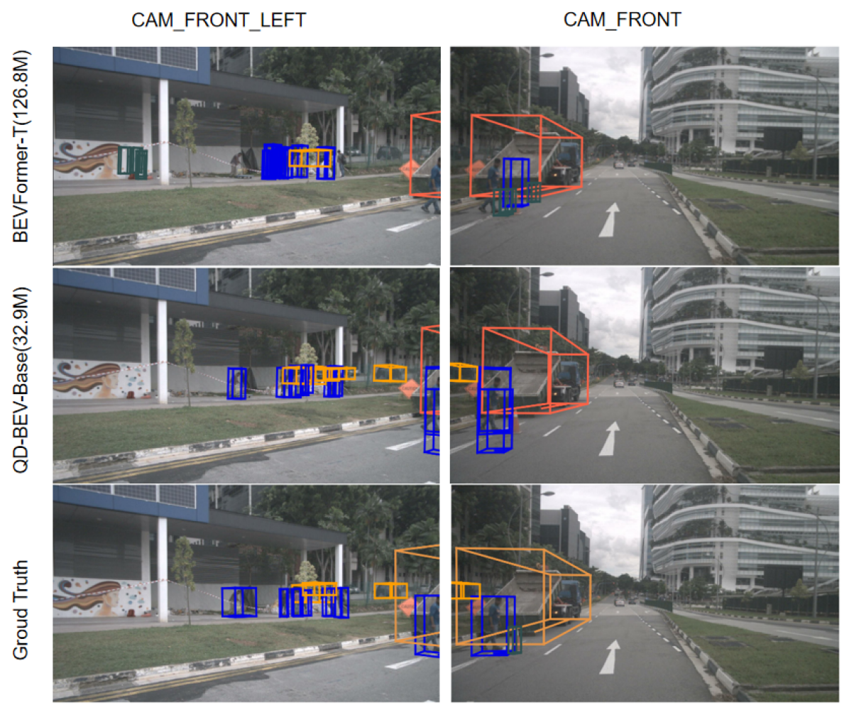
Figure 4: Visualization of QD-BEV results and the comparison with results obtained by BEVFormer.

4.4 Streaming perception result

In the context of autonomous driving, streaming perception [19] is critical for enabling models to make rapid and precise decisions in real time. High latency will degrade the streaming perception because it will cause a delay between the sensory data and the neural network output. To enhance streaming perception, quantization is a necessary technique that compresses the model size, reduces computational load, and accelerates the inference process. In Table 6, we demonstrate the significant impact of quantization on the sAP metric in autonomous driving scenarios. As we can see, QD-BEV models show consistent improvements in sAP compared to the floating-point counterparts and the quantized baselines.

Table 6: sAP of QD-BEV models compared to baselines.

Input Size	Model	W	A	mAP↑	sAP↑
450$\times$800	BEVFormer-T[23]	32	32	0.253	0.228
	BEVFormer-T-DFQ[29]	8	8	0.236	0.230
	QD-BEV-T (Ours)	4	6	0.255	0.251
720$\times$1280	BEVFormer-S[23]	32	32	0.370	0.249
	BEVFormer-S-DFQ[29]	8	8	0.356	0.322
	QD-BEV-S (Ours)	4	6	0.374	0.350
900$\times$1600	BEVFormer-B[23]	32	32	0.416	0.136
	BEVFormer-B-DFQ[29]	8	8	0.384	0.290
	QD-BEV-B (Ours)	4	6	0.406	0.337

5 Ablation study

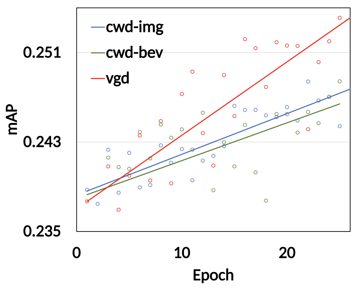
(a) mAP curve.

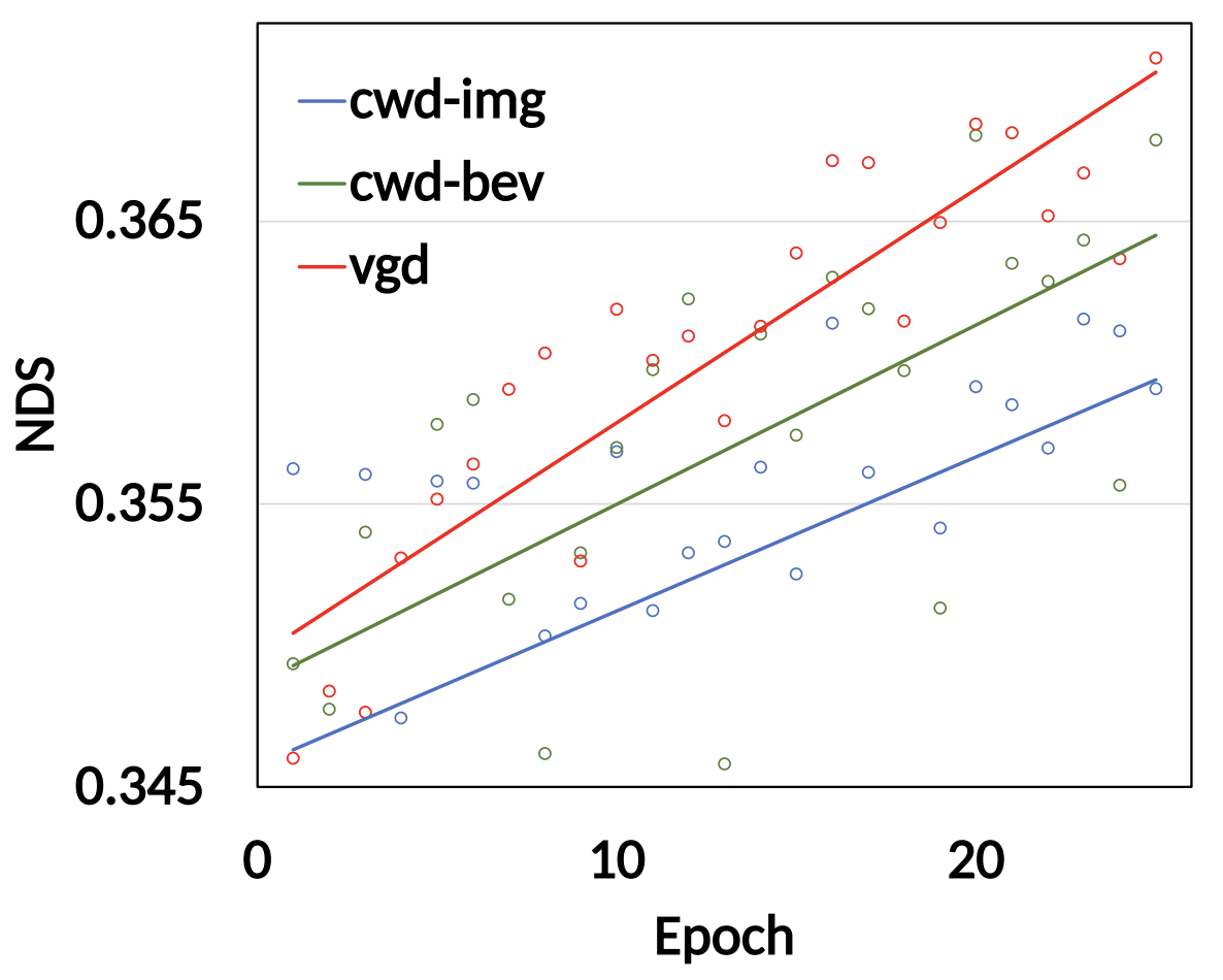
(b) NDS curve.

Figure 5: The training curve of VGD versus CWD [33]. CWD uses only one type of features, referred to as cwd-img (image feature) and cwd-bev (bev feature), respectively.

In Figure 5, we conduct an ablation study where we compare view-guided distillation with the cases using only distillation on the image feature, and only on the BEV feature, respectively. The method is referred to as CWD [33]. For a fair comparison, we apply the same pre-training weights and hyperparameters such as the temperature and the learning rate. From the figure, it can be found that view-guided distillation has a clear advantage over the CWD methods. In both the mAP and NDS curves, VGD has a more obvious and stable upward trend, and achieves better final results.

6 Conclusion

In this work, we systematically study both PTQ and QAT on BEV networks and showcase the major problems they are facing. Based on our analyses, we propose a view-guided distillation (VGD) method that can stabilize the QAT process and enhance the final performance by leveraging information from both the image domain and the BEV domain. With VGD as a plug-and-play function that can be jointly applied when quantizing BEV models, QD-BEV can close the accuracy gap or even outperforms the floating-point baselines. On the nuScenes datasets, the 4-bit weight and 6-bit activation quantized QD-BEV-Tiny model achieves 37.2% NDS with only 15.8 MB model size, outperforming BevFormer-Tiny by 1.8% with an 8$\times$ model compression.

7 Acknowledgement

This work was supported by the National Key R&D Program of China (2022ZD0116305). The authors would also like to express their gratitude to the CCF-Baidu Open Fund Project, Berkeley Deep Drive, and Intel Corporation for their support and assistance throughout this research. Special thanks to Yandong Guo from AI² Robotics (YANDONG.guo@live.com) for his valuable contributions to this work.

References

- [1] Sungsoo Ahn, Shell Xu Hu, Andreas Damianou, Neil D Lawrence, and Zhenwen Dai. Variational information distillation for knowledge transfer. In Proceedings of the IEEE/CVF Conference on Computer Vision and Pattern Recognition, pages 9163–9171, 2019.
- [2] Yoshua Bengio, Nicholas Léonard, and Aaron Courville. Estimating or propagating gradients through stochastic neurons for conditional computation. arXiv preprint arXiv:1308.3432, 2013.
- [3] Holger Caesar, Varun Bankiti, Alex H Lang, Sourabh Vora, Venice Erin Liong, Qiang Xu, Anush Krishnan, Yu Pan, Giancarlo Baldan, and Oscar Beijbom. nuscenes: A multimodal dataset for autonomous driving. In Proceedings of the IEEE/CVF conference on computer vision and pattern recognition, pages 11621–11631, 2020.
- [4] Yaohui Cai, Zhewei Yao, Zhen Dong, Amir Gholami, Michael W. Mahoney, and Kurt Keutzer. ZeroQ: A novel zero shot quantization framework. In Proceedings of the IEEE/CVF Conference on Computer Vision and Pattern Recognition, pages 13169–13178, 2020.
- [5] Nicolas Carion, Francisco Massa, Gabriel Synnaeve, Nicolas Usunier, Alexander Kirillov, and Sergey Zagoruyko. End-to-end object detection with transformers. In European conference on computer vision, pages 213–229. Springer, 2020.
- [6] Zehui Chen, Zhenyu Li, Shiquan Zhang, Liangji Fang, Qinhong Jiang, and Feng Zhao. Bevdistill: Cross-modal bev distillation for multi-view 3d object detection. arXiv preprint arXiv:2211.09386, 2022.
- [7] Jungwook Choi, Zhuo Wang, Swagath Venkataramani, Pierce I-Jen Chuang, Vijayalakshmi Srinivasan, and Kailash Gopalakrishnan. PACT: Parameterized clipping activation for quantized neural networks. arXiv preprint arXiv:1805.06085, 2018.
- [8] Elliot J Crowley, Gavin Gray, and Amos J Storkey. Moonshine: Distilling with cheap convolutions. In NeurIPS, pages 2893–2903, 2018.
- [9] Zhen Dong, Zhewei Yao, Daiyaan Arfeen, Amir Gholami, Michael W. Mahoney, and Kurt Keutzer. HAWQ-V2: Hessian aware trace-weighted quantization of neural networks. Advances in neural information processing systems, 2020.
- [10] Zhen Dong, Zhewei Yao, Amir Gholami, Michael W. Mahoney, and Kurt Keutzer. HAWQ: Hessian AWare Quantization of neural networks with mixed-precision. In The IEEE International Conference on Computer Vision (ICCV), October 2019.
- [11] Amir Gholami, Sehoon Kim, Zhen Dong, Zhewei Yao, Michael W Mahoney, and Kurt Keutzer. A survey of quantization methods for efficient neural network inference. arXiv preprint arXiv:2103.13630, 2021.
- [12] Geoffrey Hinton, Oriol Vinyals, and Jeff Dean. Distilling the knowledge in a neural network. arXiv preprint arXiv:1503.02531, 2015.
- [13] Junjie Huang and Guan Huang. Bevdet4d: Exploit temporal cues in multi-camera 3d object detection. arXiv preprint arXiv:2203.17054, 2022.
- [14] Junjie Huang, Guan Huang, Zheng Zhu, and Dalong Du. Bevdet: High-performance multi-camera 3d object detection in bird-eye-view. arXiv preprint arXiv:2112.11790, 2021.
- [15] Qijing Huang, Dequan Wang, Zhen Dong, Yizhao Gao, Yaohui Cai, Tian Li, Bichen Wu, Kurt Keutzer, and John Wawrzynek. Codenet: Efficient deployment of input-adaptive object detection on embedded fpgas. In The 2021 ACM/SIGDA International Symposium on Field-Programmable Gate Arrays, pages 206–216, 2021.
- [16] Benoit Jacob, Skirmantas Kligys, Bo Chen, Menglong Zhu, Matthew Tang, Andrew Howard, Hartwig Adam, and Dmitry Kalenichenko. Quantization and training of neural networks for efficient integer-arithmetic-only inference. In Proceedings of the IEEE Conference on Computer Vision and Pattern Recognition, pages 2704–2713, 2018.
- [17] Sehoon Kim, Coleman Hooper, Amir Gholami, Zhen Dong, Xiuyu Li, Sheng Shen, Michael W Mahoney, and Kurt Keutzer. Squeezellm: Dense-and-sparse quantization. arXiv preprint arXiv:2306.07629, 2023.
- [18] Alex H Lang, Sourabh Vora, Holger Caesar, Lubing Zhou, Jiong Yang, and Oscar Beijbom. Pointpillars: Fast encoders for object detection from point clouds. In Proceedings of the IEEE/CVF conference on computer vision and pattern recognition, pages 12697–12705, 2019.
- [19] Mengtian Li, Yu-Xiong Wang, and Deva Ramanan. Towards streaming perception. In Computer Vision–ECCV 2020: 16th European Conference, Glasgow, UK, August 23–28, 2020, Proceedings, Part II 16, pages 473–488. Springer, 2020.
- [20] Yinhao Li, Han Bao, Zheng Ge, Jinrong Yang, Jianjian Sun, and Zeming Li. Bevstereo: Enhancing depth estimation in multi-view 3d object detection with dynamic temporal stereo. arXiv preprint arXiv:2209.10248, 2022.
- [21] Yinhao Li, Zheng Ge, Guanyi Yu, Jinrong Yang, Zengran Wang, Yukang Shi, Jianjian Sun, and Zeming Li. Bevdepth: Acquisition of reliable depth for multi-view 3d object detection. arXiv preprint arXiv:2206.10092, 2022.
- [22] Yuncheng Li, Jianchao Yang, Yale Song, Liangliang Cao, Jiebo Luo, and Li-Jia Li. Learning from noisy labels with distillation. In Proceedings of the IEEE International Conference on Computer Vision, pages 1910–1918, 2017.
- [23] Zhiqi Li, Wenhai Wang, Hongyang Li, Enze Xie, Chonghao Sima, Tong Lu, Qiao Yu, and Jifeng Dai. Bevformer: Learning bird’s-eye-view representation from multi-camera images via spatiotemporal transformers. arXiv preprint arXiv:2203.17270, 2022.
- [24] Yingfei Liu, Tiancai Wang, Xiangyu Zhang, and Jian Sun. Petr: Position embedding transformation for multi-view 3d object detection. arXiv preprint arXiv:2203.05625, 2022.
- [25] Yingfei Liu, Junjie Yan, Fan Jia, Shuailin Li, Qi Gao, Tiancai Wang, Xiangyu Zhang, and Jian Sun. Petrv2: A unified framework for 3d perception from multi-camera images. arXiv preprint arXiv:2206.01256, 2022.
- [26] Yijiang Liu, Huanrui Yang, Zhen Dong, Kurt Keutzer, Li Du, and Shanghang Zhang. Noisyquant: Noisy bias-enhanced post-training activation quantization for vision transformers. In Proceedings of the IEEE/CVF Conference on Computer Vision and Pattern Recognition, pages 20321–20330, 2023.
- [27] Zhenhua Liu, Yunhe Wang, Kai Han, Wei Zhang, Siwei Ma, and Wen Gao. Post-training quantization for vision transformer. Advances in Neural Information Processing Systems, 34:28092–28103, 2021.
- [28] Asit Mishra and Debbie Marr. Apprentice: Using knowledge distillation techniques to improve low-precision network accuracy. arXiv preprint arXiv:1711.05852, 2017.
- [29] Markus Nagel, Mart van Baalen, Tijmen Blankevoort, and Max Welling. Data-free quantization through weight equalization and bias correction. In Proceedings of the IEEE/CVF International Conference on Computer Vision, pages 1325–1334, 2019.
- [30] Wonpyo Park, Dongju Kim, Yan Lu, and Minsu Cho. Relational knowledge distillation. In Proceedings of the IEEE/CVF Conference on Computer Vision and Pattern Recognition, pages 3967–3976, 2019.
- [31] Jonah Philion and Sanja Fidler. Lift, splat, shoot: Encoding images from arbitrary camera rigs by implicitly unprojecting to 3d. In European Conference on Computer Vision, pages 194–210. Springer, 2020.
- [32] Antonio Polino, Razvan Pascanu, and Dan Alistarh. Model compression via distillation and quantization. arXiv preprint arXiv:1802.05668, 2018.
- [33] Changyong Shu, Yifan Liu, Jianfei Gao, Zheng Yan, and Chunhua Shen. Channel-wise knowledge distillation for dense prediction. In Proceedings of the IEEE/CVF International Conference on Computer Vision, pages 5311–5320, 2021.
- [34] Antti Tarvainen and Harri Valpola. Mean teachers are better role models: Weight-averaged consistency targets improve semi-supervised deep learning results. arXiv preprint arXiv:1703.01780, 2017.
- [35] Mart van Baalen, Christos Louizos, Markus Nagel, Rana Ali Amjad, Ying Wang, Tijmen Blankevoort, and Max Welling. Bayesian bits: Unifying quantization and pruning. Advances in neural information processing systems, 2020.
- [36] Kuan Wang, Zhijian Liu, Yujun Lin, Ji Lin, and Song Han. HAQ: Hardware-aware automated quantization. In Proceedings of the IEEE conference on computer vision and pattern recognition, 2019.
- [37] Peisong Wang, Qiang Chen, Xiangyu He, and Jian Cheng. Towards accurate post-training network quantization via bit-split and stitching. In International Conference on Machine Learning, pages 9847–9856. PMLR, 2020.
- [38] Yue Wang, Vitor Campagnolo Guizilini, Tianyuan Zhang, Yilun Wang, Hang Zhao, and Justin Solomon. Detr3d: 3d object detection from multi-view images via 3d-to-2d queries. In Conference on Robot Learning, pages 180–191. PMLR, 2022.
- [39] Lirui Xiao, Huanrui Yang, Zhen Dong, Kurt Keutzer, Li Du, and Shanghang Zhang. Csq: Growing mixed-precision quantization scheme with bi-level continuous sparsification. arXiv preprint arXiv:2212.02770, 2022.
- [40] Zhewei Yao, Zhen Dong, Zhangcheng Zheng, Amir Gholami, Jiali Yu, Eric Tan, Leyuan Wang, Qijing Huang, Yida Wang, Michael Mahoney, et al. Hawq-v3: Dyadic neural network quantization. In International Conference on Machine Learning, pages 11875–11886. PMLR, 2021.
- [41] Shan You, Chang Xu, Chao Xu, and Dacheng Tao. Learning from multiple teacher networks. In Proceedings of the 23rd ACM SIGKDD International Conference on Knowledge Discovery and Data Mining, pages 1285–1294, 2017.
- [42] Dongqing Zhang, Jiaolong Yang, Dongqiangzi Ye, and Gang Hua. LQ-Nets: Learned quantization for highly accurate and compact deep neural networks. In The European Conference on Computer Vision (ECCV), September 2018.
- [43] Linfeng Zhang, Jiebo Song, Anni Gao, Jingwei Chen, Chenglong Bao, and Kaisheng Ma. Be your own teacher: Improve the performance of convolutional neural networks via self distillation. In Proceedings of the IEEE/CVF International Conference on Computer Vision, pages 3713–3722, 2019.
- [44] Lingran Zhao, Zhen Dong, and Kurt Keutzer. Analysis of quantization on mlp-based vision models. arXiv preprint arXiv:2209.06383, 2022.
- [45] Aojun Zhou, Anbang Yao, Yiwen Guo, Lin Xu, and Yurong Chen. Incremental network quantization: Towards lossless cnns with low-precision weights. arXiv preprint arXiv:1702.03044, 2017.
- [46] Yiren Zhou, Seyed-Mohsen Moosavi-Dezfooli, Ngai-Man Cheung, and Pascal Frossard. Adaptive quantization for deep neural network. arXiv preprint arXiv:1712.01048, 2017.
- [47] Yin Zhou and Oncel Tuzel. Voxelnet: End-to-end learning for point cloud based 3d object detection. In Proceedings of the IEEE conference on computer vision and pattern recognition, pages 4490–4499, 2018.
- [48] Xizhou Zhu, Weijie Su, Lewei Lu, Bin Li, Xiaogang Wang, and Jifeng Dai. Deformable detr: Deformable transformers for end-to-end object detection. arXiv preprint arXiv:2010.04159, 2020.