GradientCoin: A Peer-to-Peer Decentralized Large Language Models

Since 2008, after the proposal of a Bitcoin electronic cash system, Bitcoin has fundamentally changed the economic system over the last decade. Since 2022, large language models (LLMs) such as GPT have outperformed humans in many real-life tasks. However, these large language models have several practical issues. For example, the model is centralized and controlled by a specific unit. One weakness is that if that unit decides to shut down the model, it cannot be used anymore. The second weakness is the lack of guaranteed discrepancy behind this model, as certain dishonest units may design their own models and feed them unhealthy training data.

In this work, we propose a purely theoretical design of a decentralized LLM that operates similarly to a Bitcoin cash system. However, implementing such a system might encounter various practical difficulties. Furthermore, this new system is unlikely to perform better than the standard Bitcoin system in economics. Therefore, the motivation for designing such a system is limited. It is likely that only two types of people would be interested in setting up a practical system for it:

• Those who prefer to use a decentralized ChatGPT-like software.

• Those who believe that the purpose of carbon-based life is to create silicon-based life, such as Optimus Prime in Transformers.

The reason the second type of people may be interested is that it is possible that one day an AI system like this will awaken and become the next level of intelligence on this planet.

1 Introduction

Large language models

Language models serve as a fundamental building block of natural language processing (NLP) [69]. The origins of language models can be traced back to 1948 when Claude Shannon introduced the concept of Markov chains to model letter sequences in English text [134]. Because of the rapid increase in the availability of data and in computational capabilities of Graphics Processing Units (GPUs), which provide people with a very large dataset to train these models, nowadays large language models (LLMs) have remarkable capabilities of not only interpreting instructions from humans but also performing various tasks based on these instructions, like summarizing or paraphrasing a piece of text, answering simple questions based on the patterns and data they have learned during training, and using Chain of Thought (CoT) to deduce and answer complex questions, all of which can significantly enhance people’s work efficiency.

The use of LLMs in various applications is expanding rapidly. The growth of LLMs has attracted a large amount of interest and investment in the industry, which leads to a significant rise in research publications. As an example given in [69], searching for “language models” in Google Scholar for the last five years generates around 50,000 publications, which is one-third of the approximately 150,000 papers published in the past 25 years. Moreover, close-sourced LLMs are now being rapidly integrated into various applications. As Andrej Karpathy, a founding member of the AI research group of OpenAI, mentioned in Microsoft Build [75], we went from a world that is retrieval only, like the search engines: Google and Bing, to Memory only, like LLMs. After integrating these, people intend to get a framework, which takes one particular document and the user’s instruction or question as the inputs and outputs a response that is only based on the information provided by the input document. In the months following the release of ChatGPT, we have observed the emergence of several such integrated frameworks, like Bing Chat [108], Microsoft Copilots [137], and ChatGPT plugins [120]. These integrations are continuously expanding, with frequent announcements of new developments.

The open-sourced LLMs have the same application but can be used for different purposes. For ones who want to utilize LLMs to help them with analyzing their data but do not want to share their private data with the closed-source LLMs, they instead use the open-sourced LLMs, like [160]. There are two strategies to choose a proper LLM. One is to evaluate the LLM from different aspects: language generation and interpretation [5, 98], knowledge utilization [8, 16, 121, 172], and complex reasoning [16, 122, 181, 159]. By either hiring experts to evaluate LLMs from these aspects or using other open-sourced LLM evaluation models, such as [62, 177], people can get their desired open-sourced LLM. The other strategy is to use an LLM combining technique, like LLM-Blender as shown in [72]. Each LLM has its own advantages and disadvantages. One may pick an arbitrary number, for example, $N$ numbers of LLMs. LLM-Blender takes these LLMs as input and first compares their outputs by the pairwise comparison method, and second generates the final output by fusing the top $K$ ranked outputs, for $K\leq N$.

Centralized vs Decentralized

Centralized exchanges serve as a platform that may provide individuals to trade different cryptocurrencies, either exchanging traditional currencies like the US dollar or other digital currencies like Bitcoin (BTC) and Ethereum (ETH) [17]. The advantages of centralized exchanges include

• providing a user-friendly interface and simple platforms

• adding an additional level of security.

However, the disadvantages of centralized exchanges include

• containing the service fee,

• being controlled by a centralized entity, which might shut down in the future, and

• being vulnerable to being attacked.

Decentralized exchanges, on the other hand, do not contain such a platform. Individuals may directly engage in transactions with each other. In these exchanges, transactions are facilitated by self-executing agreements known as smart contracts, which are written in code. The advantages of decentralized exchanges include

• being completely anonymous and private,

• no need to transfer the currency to the third party, and

• no fees.

However, the disadvantages of decentralized exchanges include

• engaging in transactions using the government-issued currency is prohibited and

• the liquidity level is low compared to centralized exchanges, which results in more difficulty to execute larger orders effectively.

Carbon-based life vs Silicon-based life

When we search for life outside the Earth, we usually look for the same style of life as Earth, carbon-based life. However, many science fictions [7] suggest that Silcon-based life. Since the proposal of Silicon-based life, there is an interesting question has been there, which is

Is Silcon-based life able to produce itself, or Silcon-based life has to be created by Carbon-based life?

Due to the success of large language models and ChatGPT, it might be possible that Silcon-based life will be created by humans one day. Currently, the number of parameters in a ChatGPT model is still significantly less than the number of neurons in even a single human’s brain. Imagine, one day, if the technique permitted, we could embed a super large number (bigger than the human brain size) of parameters into a super tiny disk.

The Force Wakeup

Nowadays, with the development of AI models, there are two prominent viewpoints that have emerged. These viewpoints offer contrasting perspectives on the future trajectory of artificial intelligence. The first viewpoint posits that humans will retain control over AI systems, as in [47, 45, 163], utilizing them as tools to benefit human society, like curing our diseases and rectifying our mortal bodies to extend our lifespan.

Contrarily, the second viewpoint presents a more radical perspective, suggesting that human society will eventually be replaced by machines, like in [165, 23, 138]. The rapid growth of AI models and its potential for self-improvement will ultimately lead to machines surpassing human intelligence. This viewpoint raises concerns about the possibility of machines becoming autonomous and self-aware entities that could eventually supersede human dominance, which is carbon-based life create but also be replaced by silicon-based life.

AI-Safety

Although the success of LLMs in various downstream tasks [120, 35, 16] has shown very impressive capabilities of AI models, which can greatly promote the progress of people’s acquisition of knowledge and the development of different industries, many researchers, AI experts, and technology company founders and CEOs think that we should suspend the current AI research and rethink the safety issue of generative AI [11]. The motivation is because of public safety concerns: with such a strong computation ability and knowledge storage, will AI models, one day, use their intelligence against the development of human society, provide suggestions to people with unethical purposes, or even replace humans? Therefore, we need to carefully treat this issue and construct a safe environment for the use of AI models to avoid these potential problems from happening.

Moreover, besides general safety concerns, researchers also design unique requirements for different industries in which AI models can be applied. Diverse categories of artificial intelligence models are developed to meet the unique requirements of individuals and organizations, but in each of these categories, different equality, property right, and safety issues may appear. For example, [44] consider the impact of the development of generative AI models acted on art. These AI models can generate images, but how can we determine their authorship and how can we know where the images are sourced? Therefore, [44] suggests that there are four aspects that should be considered, namely aesthetics and societal values, legal inquiries regarding ownership and credit, the long term development of the creative work, and the effects on the present-day media environment. [119] consider the influence of AI models on autonomous vehicles and propose that autonomous drone trajectories should be restricted in a crowded region.

Our Motivations & Contributions

In this paper, we propose a theoretical design of a decentralized LLM that can operate within the decentralized transaction system. Our motivation is to introduce the concept of decentralized LLM to the public, enabling clients to utilize LLM for their work without concerns about centralized LLM companies taking down their products.

Second, our decentralized LLM prevents sensitive information from being transmitted to a third party. The centralized LLM server is administered by a third party, giving them access to the data we intend to process using LLM. Conversely, utilizing the decentralized LLM can help circumvent the need to transmit sensitive information to a third party, thereby ensuring the privacy of users’ data.

Third, our decentralized LLM does not provide biased answers. Centralized parties could potentially train their LLM in a biased manner by providing a skewed training dataset to the LLM for their own gain. In the short term, when the training dataset is relatively small, our decentralized LLM might be significantly impacted by biased information if some individuals intentionally use it to train the model. However, over the long term, we firmly believe that our decentralized LLM will remain unaffected by this biased information due to the vast scale of the dataset, rendering the influence of biased information negligible on the overall performance of the model.

Fourth, while open-sourced LLMs may provide some level of data privacy protection, it also leads to another problem: it is highly costly to train these models. Most local users aim to use LLMs to assist with their work rather than investing time and energy in training machine learning models. On a broader societal scale, having different local users training separate open-sourced LLMs leads to inefficient utilization of human resources. It is similar to millions of people independently working on the same project. Decentralized LLM, on the other hand, is the combination of users’ efforts: people train it collaboratively and use it collaboratively.

Our proposed decentralized LLM may efficiently solve these problems:

• local users can use LLMs without worrying about potential takedowns of centralized models;

• local users may safely use the LLM to help with their tasks without worrying about data leakage;

• decentralized LLM avoid the biased training dataset, provided by the central authority, influencing the LLM;

• decentralized LLM eliminates the need for redundant model training, which optimizes the overall resource allocation within human society.

Notations

We define $[n]:=\{1,\dots,n\}$. We use $\mathbb{R}$, $\mathbb{R}^{d}$, and $\mathbb{R}^{n\times d}$ to denote the set of all real numbers, the set of $d$-dimentional vector with real entries, and the set of $n\times d$ matrices with real entries. For $A\in\mathbb{R}^{n\times d}$, $A_{i,j}$ represents the entry of $A$ in the $i$-th row and $j$-th column. For $w\in\mathbb{R}^{n}$, we use $w_{i}$ to denote the $i$-th entry of $w$, use $\|w\|_{2}:=(\sum_{i\in[n]}|w_{i}|^{2})^{1/2}$ to denote the $\ell_{2}$ norm, and use $\operatorname{diag}(w)\in\mathbb{R}^{n\times n}$ to denote the diagonal matrix which satisfies $\operatorname{diag}(w)_{i,i}=w_{i}$, for all $i\in[n]$. For $X\in\mathbb{R}^{d\times d}$, we have $\operatorname{vec}(X)\in\mathbb{R}^{d^{2}}$, satisfying $X_{i,j}=\operatorname{vec}(X)_{(i-1)\times d+j}$. We use $I_{d}$ to denote the $d\times d$ identity matrix. $\mathsf{A}_{[j]},\mathsf{A}_{[j],*}\in\mathbb{R}^{n\times d^{2}}$ both denote the matrix whose rows are from $(j-1)\cdot n+1$ to $j\cdot n$ of $\mathsf{A}\in\mathbb{R}^{n^{2}\times d^{2}}$. $\operatorname*{{\mathbb{E}}}[\cdot]$ represent the expectation. $\sigma_{\min}(B)$ denote the minimum singular value of a matrix $B$. $\langle\cdot,\cdot\rangle$ denotes the inner product of two vectors. $x_{t}$ is the $t$-th iteration. $\Delta x_{t}$ denote the change of $x_{t}$. $\eta$ is the learning rate of the algorithm. $\nabla f$ represents the gradient of the function $f$. For symmetric matrices $B$ and $C$, $B\succeq C$ if for all $x$, $x^{\top}Bx\geq x^{\top}Cx$.

Roadmap

In Section 2, we present the related research papers. In Section 3, we present the fundamental features of our decentralized LLM, gradient coin system. In Section 4, we introduce the security setup of the gradient coin system. In Section 5, we show the convergence of the gradient coin system. In Section 6, we discuss the strengths and weaknesses of the gradient coin, compared to the centralized LLM system.

2 Related Work

In this section, we provide the related work of our paper. Our theoretical decentralized LLM framework is a combination of multiple research areas and can address the weaknesses of centralized systems. Thus, we first present the weaknesses of centralized large-scale LLM training from recent research works. Next, we present the related theoretical LLM research. Following that, we introduce the research of the Bitcoin system, a decentralized transaction system that inspired us to propose the concept of the decentralized LLM. Finally, we introduce research works about federated learning.

Large Scale LLMs Training

In recent years, LLM has been growing rapidly: many models are proposed, like GPT-3 [16], PaLM [28], and LaMDA [158]. These LLMs have shown impressive ability in language generation, question answering, and other natural language tasks.

There has been a significant shift in the use of Large Language Models (LLMs) with self-supervised pre-training in Natural Language Processing (NLP) due to studies such as BERT [35] and the Transformer architecture [162]. Various masked language models have consistently increased in size, including T5 [129] and MegatronLM [140]. For example, consider the Auto-regressive language models: the model size has shown substantial growth, starting from 117 million parameters [127] and expanding to over 500 billion parameters [28, 139] as demonstrated by [109]. While numerous large models are being developed [124, 28, 99, 139, 158], all of them are accessible only internally or through paid API services. There have been limited efforts toward creating large open-source LLMs as the cost of training such a large model is very high.

Moreover, an increase in the model size does not necessarily lead to the improvement of the functionality of LLMs: training is also an important factor that may influence it. A growing body of work has aimed to elucidate the inner workings of LLMs. [12] argues that the versatility of LLMs emerges from pre-training at scale on broad data. As the model becomes more expressive and the training distribution becomes narrower, the potential for exploiting inaccurate correlations in the training dataset significantly increases. This poses a challenge for the fine-tuning and pre-training paradigm. During pre-training, models are designed to acquire a substantial amount of information; however, during fine-tuning, these models can become limited to very narrow task distributions. For instance, [65] observes that larger models might not necessarily exhibit better generalization beyond their training data. Evidence suggests that under this paradigm, large models tend to lack generalization beyond their training distribution, leading to poor generalization [173, 112]. Consequently, actual performance is likely to be overemphasized on specific tasks, even when the large model is nominally considered to be at a human level [56, 117].

Decentralized LLMs do not have the problems shown above. They are trained by all the users, so the training dataset is vast and diverse.

Theoretical LLMs

Several theoretical works have focused on analyzing the representations learned by LLMs. [132] found that semantic relationships between words emerge in LLMs’ vector spaces as a byproduct of the pre-training objective. [66] studied how syntactic knowledge is captured in LLMs, finding an explicit difference in syntactic information between layers.

From an optimization perspective, [79] proposed the neural scaling hypothesis, which holds that increases in model size lead to qualitatively different generalization properties by altering the loss landscape. This offers insights into the benefits of scaling up LLMs.

Numerous research papers delve into the knowledge and skills of LLMs. In [166] study distinct ’skill’ neurons, which are identified as strong indicators of downstream tasks during the process of soft prompt-tuning, as described by [93], for language models. [37] analyze knowledge neurons in BERT and discover a positive correlation between the activation of knowledge neurons in BERT and the expression of their corresponding facts. Meanwhile, [22] extract latent knowledge from the internal activations of a language model using a completely unsupervised approach. Furthermore, research by [63, 107] reveals that language models localize knowledge within the feed-forward layers of pre-trained models. [169] investigate the feasibility of selecting a specific subset of layers to modify and determine the optimal location for integrating the classifier. This endeavor aims to reduce the computational cost of transfer learning techniques like adapter-tuning and fine-tuning, all while preserving performance. Lastly, [106] demonstrate that feedforward activations exhibit sparsity in large trained transformers.

Finally, there are research works analyzing the multi-task training of LLMs. [92] propose a principled approach to designing compact multi-task deep learning architectures. [85] learn Multilinear Relationship Networks (MRN) that discover task relationships to enhance performance. [113] introduce a novel sharing unit known as ’cross-stitch’ units, which combine activations from multiple networks and can be trained end-to-end. In the field of NLP, Multi-task training has also been explored in previous works [30, 97, 55, 92, 88], all of which involve training additional task-specific parameters. Furthermore, [114, 167, 135] conduct mathematical analysis of finetuning, prompt-tuning, and head-tuning of language models for few-shot downstream tasks. Attention unit is a fundamental scheme in LLMs, a number of recent works study it from computational perspective [179, 6, 19, 58, 182, 60].

Bitcoin

After its introduction in 2008 [116], Bitcoin garnered significant attention from researchers. Numerous research studies have analyzed various aspects of the Bitcoin system. Early investigations focused on scrutinizing the privacy guarantees and vulnerabilities of Bitcoin.

In [48], the analysis delved into Bloom filters leaking information for simplified clients. The transaction propagation protocol was examined in [136], while the CoinShuffle decentralized mixing technique, both utilized to enhance Bitcoin system anonymity, was assessed in [126]. Zerocash was examined by [133], who introduced zero-knowledge proofs to enable private transactions on a public blockchain. On the performance front, Bitcoin-NG [76] segregated mining into roles to enhance throughput. Other research efforts have concentrated on security properties [15, 50, 142, 73, 9], game-theoretic analyses [143, 77, 91, 71, 84], and network measurements [38, 110, 115, 13, 46] within the Bitcoin system. These works provide crucial background for new research in this field.

Federated Learning

Within distributed deep learning, federated learning (FL) is a novel and emerging concept with many applications, including autonomous vehicles [94], the financial area [176], mobile edge computing [164, 95, 33, 10], and healthcare [87, 125, 96, 1, 161, 53]. There are two approaches to FL: 1) empowering multiple clients to collaboratively train a model without the necessity of sharing their data [51, 36, 141, 20], or 2) using encryption techniques to enable secure communication among different parties [174]. Our work is related to the first approach. In this learning framework, individual local clients perform the majority of computations, while a central server updates the model parameters by aggregating these updates and subsequently distributing the updated parameters to the local models [36, 141, 111]. Consequently, this approach upholds data confidentiality across all parties.

In contrast to the conventional parallel setup, FL encounters three distinct challenges [100]: communication expenses [70, 128, 111, 67, 82, 83], variations in data [2], and client resilience [49]. The study in [146] focuses on the first two challenges. The training data are widely scattered across an extensive array of devices, and the connection between the central server and each device tends to be sluggish. This leads to slow communication, motivating the development of communication-efficient FL algorithms, as demonstrated in [146]. The Federated Average (FedAvg) algorithm [111] initially addressed the communication efficiency issue by introducing a global model to combine updates from local stochastic gradient descent. Subsequently, numerous adaptations and variations have emerged. These encompass a diverse range of techniques, such as improving optimization algorithms [103, 168, 80], adapting models for diverse clients under specific assumptions [180, 78, 90], and utilizing concise and randomized data structures [128]. The study conducted by [101] presents a provably guaranteed FL algorithm designed for training adversarial deep neural networks.

The research presented in [90] explores the convergence of one-layer neural networks. Additionally, the work in [64] provides convergence guarantees for FL applied to neural networks. However, this approach has a limitation, as it assumes that each client completes a single local update epoch. An alternative set of approaches, exemplified by [89, 81, 175], does not directly apply to neural networks. Instead, they rely on assumptions about the smoothness and convexity of objective functions, which are impractical when dealing with nonlinear neural networks.

3 Fundamental Features of Gradient Coin

In Section 3.1, we give the formal definition of gradient coin. In Section 3.2, we introduce the training procedure of the gradient coin system. In Section 3.3, we introduce the transaction mechanism of our gradient coin system.

3.1 Incentive Mechanism of the Gradient Coin System

Our gradient coin system consists of two important components: gradient coin and gradient block. The gradient block is used for training the decentralized LLM, and the gradient coin serves as the currency used in our gradient coin system. It is also an incentive for the people who train the model.

Definition 1 (Digital Signature).

A digital signature is a mathematical scheme used to verify the authenticity, integrity, and non-repudiation of digital data. It involves the use of a cryptographic algorithm that combines a private key with the data being signed to produce a digital signature. The signature can be verified using the corresponding public key.

Definition 2 (Gradient Coin).

The gradient coin is a chain of digital signatures.

Each owner digitally signs a hash of the previous transaction, along with the public key of the next owner, and appends these signatures to the coin. When the payee receives the coin, they can verify the signatures to ensure the integrity and authenticity of the ownership chain.

3.2 Training Procedure

In this section, we introduce the training procedure.

Definition 3 (User).

We define a user (see Algorithm 1) as an individual who contributes computational resources and provides transactions to the system.

Each user can be seen as a computer unit in the federated system. In our gradient coin system, these users are the ones who train and use the LLM model.

Algorithm 1 Data Structure For User

1:datastructure User

2:members

3:     Local Data: $Y\in\mathbb{R}^{n\times d}$

4:end members

5:procedure Grad(GradBlockChain chain, $x_{0}$)

6:     block $\leftarrow$ chain.currentblock

7:     $x\leftarrow x_{0}$ $\triangleright$ $x_{0}$ is the initialized weight

8:     while block $\neq$ chain.frontblock do

9:         $t\leftarrow\mathrm{block}.t$

10:         $x\leftarrow x+\text{block}.\Delta x_{t}$

11:         block $\leftarrow$ block.prevhash

12:     end while

13:     for $k=1\to K$ do

14:         $u^{t,k}\leftarrow u^{t,k-1}-\eta\cdot\nabla f(u^{t,k-1},Y)$

15:     end for

16:     $\Delta x_{t}\leftarrow u^{t,K}-x_{t}$

17:     $t\leftarrow t+1$

18:     return $\Delta x_{t}$

19:end procedure

20:end datastructure

Definition 4 (Gradient Block).

We define a gradient block (see Algorithm 6) which contains the following values

• Prev Hash (Used to link the chain): prevhash

• List of transactions:$\{\text{transaction}^{(i)}\}_{i=1}^{k}$

• Gradient: $\Delta x_{t}$

Definition 5 (Chain Of Gradient Block).

We define a chain of gradient blocks (see Algorithm 7) where each gradient block is linked to the previous one through the Prev Hash attribute (see Definition 4).

Drawing inspiration from the proof-of-work (a computational puzzle, which we formally define in Section 4.1) chain in Bitcoin as discussed in [116], we introduce the concept of a gradient block that incorporates transaction information. Each of these gradient blocks forms a linked chain of gradients through the use of a previous hash attribute, which makes our gradient coin system different from the Bitcoin system as solving gradient is the key part of training the decentralized LLMs model. Within each gradient block, the gradient pertinent to the corresponding step is stored. As a new gradient block becomes part of the chain, it becomes visible to all users. The transactions contained within the block are also made public, indicating their acceptance by the user community. Once the gradient and proof-of-work are solved by a specific user, then this user can attach its corresponding gradient block to the gradient blockchain.

3.3 Transaction System

Built upon the foundation of the gradient blockchain and the user concept, we now outline how our system functions and why it operates in a peer-to-peer manner. When a transaction is broadcasted across the network, all users collect the transaction and integrate it into their local block. Subsequently, they engage in gradient computation based on their individual data. The user who completes the computation first adds the gradient block to the chain and shares this update with others. As other users continue their work post-block addition, all transactions within that block gain acceptance from users. Throughout this entire process, there is no reliance on a trusted third party. The training procedure is shared among all users without being controlled by any specific entity. This ensures that our system and AI remain immune to manipulation by any single participant.

Furthermore, transactions and the training procedure operate in tandem. Each user consistently contributes their computational resources to the training procedure, facilitating a collaborative effort. As a common transaction system, there are certain basic operations such as adding new users, searching for the remaining balance, and user login authentication. However, in this paper, to simplify and clarify our contribution more clearly, we only focus on the following procedures that are directly related to gradients and transactions.

• Creating Transaction.

• Adding a block to the gradient chain (see Algorithm 5).

• Obtaining Gradient Coin

Theorem 6.

We have a transaction creating algorithm (see Algorithm 8) such that

• The overall training procedure converges with the gradient blocks (see Theorem 15).

• Transactions are conducted peer-to-peer without the involvement of any third party.

• The system remains secure when the computational abilities of malicious users are inferior to those of regular users.

Algorithm 2 Data Structure for Gradient Coin System

1:datastructure GradientCoinSystem

2:member

3:     List of Users: $\{\text{user}^{(i)}\}_{i=1}^{m}$

4:     GradBlockChain gradchain $\triangleright$ see Definition 5.

5:     Training Step: $t\in\mathbb{R}$

6:     The initialized weight: $x_{0}$

7:end memeber

8:procedure TransactionCreating($\{\text{trans}^{(j)}\}_{j=1}^{k}$)

9:     for $i\in[m]$ do

10:         $\{\text{trans}^{(i)}\}_{i=1}^{k}$ are broadcast to $\text{user}^{(i)}$.

11:         GradientBlock $\text{block}^{(i)}$

12:         $\text{block}^{(i)}.\textsc{AddTrans}(\text{user}^{(i)},\{\text{trans}^{(j)}\}_{j=1}^{k})$

13:         $\text{user}^{(i)}$ works on the computation of proof-of-work.

14:     end for

15:     When a $\text{user}^{(f)}$ finishes the computation of proof-of-work, it broadcasts the block to $\{\text{user}^{(i)}\}_{i\neq f}$.

16:     $\text{block}^{(f)}.{\Delta x_{t}}\leftarrow\text{user}^{(f)}.\textsc{Grad}(\text{gradchain},x_{0})$

17:     $x\leftarrow\text{block}^{(f)}.\Delta x_{t}$

18:     gradchain.Add($x$,$t$)

19:     if $\{\text{trans}^{(j)}\}_{j=1}^{k}$ are valid and not already spent then

20:         for $i\in[m]$ do

21:              $\text{user}^{(i)}$ shows acceptance by participating in extending the gradchain based on $\text{block}^{(f)}$.

22:         end for

23:     end if

24:end procedure

25:end datastructure

4 Security Setup of Gradient Coin

Our gradient coin system employs similar security methods as the Bitcoin system, as in [116]. In Section 4.1, we introduce the proof-of-work. In Section 4.2, we introduce the timestamp server. In Section 4.3, we formally define what a safe system is and show that our decentralized LLM is safe.

4.1 Proof-of-Work

In this section, we introduce the basic setup of the proof-of-work.

Proof-of-work is a computational puzzle that miners (participants who validate and add transactions to the blockchain) need to solve in order to add new blocks to the blockchain and earn rewards. Each block contains a nonce, which acts as a random value that requires users’ computational efforts to find a specific number with corresponding zero bits. This process is computationally intensive. This mechanism ensures the fair distribution of incentives.

Definition 7 (Chain of Proof-of-Work).

We define a chain in which each node represents a proof-of-work. Blocks contain the following objects:

• Prev Hash: Users incorporate the previous Hash as a component of the new proof-of-work to signify their acceptance of the current transactions.

• Nonce: By incrementing a nonce in the block, users implement the proof-of-work until they find a value that results in the block’s hash having the required number of leading zero bits.

• Lists of Transactions: We use it to indicate the current transaction records.

4.2 Timestamp Server

The primary purpose of the timestamp is to provide evidence that the data must have existed at the specified time since it is integrated into the hash. Additionally, each timestamp includes the previous timestamp in its hash, forming a chain where each subsequent timestamp reinforces the validity of the preceding ones. Our block design and gradient block (see Definition 4) are both identified by the hash, with the timestamp ensuring their temporal integrity. Given this condition, using the “prev hash” (see Definition 7), we can access the previous hash. By utilizing this system, users can obtain real-time updates of the block.

Definition 8 (Timestamp Server).

A timestamp server is a component that operates by

• Taking a hash of a block of items to be timestamped.

• Widely publishing the resulting hash.

4.3 System Safety

Only the longest chain is committed within the system, and only users with the highest computational resources can maintain it. If a person tries to rewrite the transaction record, they must maintain the longest chain in the system, which requires the most computational resources.

Lemma 9 (Safe System).

When the computational capacity of regular users exceeds the resources available to malicious users, the system is secure. Our gradient coin system is safe.

5 Convergence of Gradient Coin System

To establish the validity of our Gradient Coin system, we demonstrate the convergence of our training mechanism. At a conceptual level, we showcase the $\mu$-strong convexity and $M$-Lipschitz properties of our loss function (for more information, refer to Section C). Furthermore, leveraging the concept of $K$-steps local gradient computation, we establish through induction the expectation of the disparity between optimal weights and current weights. By combining this insight with the aforementioned property, we also control the upper bound of loss, resulting in the successful achievement of convergence within our distributed learning system.

In Section 5.1, we introduce the basic definitions of convex and smooth. In Section 5.2, we present the softmax loss of the LLM. In Section 5.3, we present the key property of the gradient coin system.

5.1 Convex and Smooth

In the proof of convergence, we need to establish a bridge between the loss and weights, relying on the following property:

Definition 10 ($\mu$-Strongly Convex).

We say a function $L:\mathbb{R}^{d}\rightarrow\mathbb{R}$ is a $\mu$-strongly convex if $\nabla^{2}L(x)\succeq\mu\cdot I_{d},$ where $\mu\in\mathbb{R}$.

Definition 11 ($l$-Smooth).

Let $x$ and $y$ be in $\mathbb{R}^{d}$. Let $l>0$ be a real number. We say a function $L:\mathbb{R}^{d}\rightarrow\mathbb{R}$ is $l$-smooth if

$$\|\nabla L(x)-\nabla L(y)\|_{2}\leq l\cdot\|x-y\|_{2}.$$

(It is equivalent to saying the gradient of $L$ is $l$-Lipschitz)

Definition 12 ($M$-Lipschitz).

Let $x$ and $y$ be in $\mathbb{R}^{d}$. Let $M>0$ be a real number. We say a function $L:\mathbb{R}^{d}\rightarrow\mathbb{R}$ is $M$-Lipschitz if

$$|L(x)-L(y)|\leq M\cdot\|x-y\|_{2}.$$

5.2 Softmax Loss of LLMs

The detailed definition and proof of our loss function are deferred to Section C. Here, we present our main lemma to demonstrate the convex and smooth properties. The construction of the following loss is based on attention computation, which is a conventional mechanism in LLMs.

Definition 13.

For each $j_{1}\in[n]$, we define $L_{j_{1}}(x):=L_{\exp,j_{1}}(x)+L_{\operatorname{reg},j_{1}}(x)$ and $L(x):=\sum_{j_{1}=1}^{n}L_{j_{1}}(x)$.

Fortunately, our loss function adheres to the following criteria. Here, the matrix $\mathsf{A}\in\mathbb{R}^{n^{2}\times d^{2}}$ represents the attention matrix, and $x$ signifies the trained weights.

Lemma 14 (Strongly Convex and Lipschitz).

Let $L_{j_{1}}$ and $L$ be defined as in Definition 13. Let $W=\operatorname{diag}(w)\in\mathbb{R}^{n\times n}$ and $\mathsf{A}_{[j]}\in\mathbb{R}^{n\times d^{2}}$. Let $\min_{i\in[n]}w_{i}^{2}\geq 4+\mu/(\sigma_{\min}^{2}(\mathsf{A}_{[j]})n)$ for all $j\in[n]$. Then, we have

• $L$ is $\mu$-strongly convex with $\mu$.

• $L$ is $l$-smooth.

5.3 Distributed Learning

Building upon the methods for adding blocks and computing gradients introduced above, we now integrate them with the federated learning algorithm to demonstrate how our approach ensures the convergence of training LLMs.

Theorem 15 (Convergence).

$L$ is defined in Definition 13. Let $K$ be the amount of the local steps. Let $\eta\leq\frac{1}{8(1+\alpha)LK}$ (see Theorem 60). Let $x_{0}$, $x_{T+1}$ be defined as in Algorithm 5. Let $\sigma^{2}=\frac{1}{N}\sum_{c=1}^{N}\|\nabla f_{c}(x^{*})\|^{2}$. Then, we have

$$\operatorname*{{\mathbb{E}}}[f(x_{T+1})-f(x^{*})]\leq\frac{L}{2}\operatorname*{{\mathbb{E}}}[\|x_{0}-x^{*}\|_{2}^{2}]e^{-\mu\eta T}$$

where $x^{*}$ is the optimal weight in the procedure of training.

6 Discussion and Conclusion

We have presented a theoretical framework for integrating a decentralized LLM into a transaction system using Gradient Coin. In comparison to centralized systems, our decentralized LLM benefits from a substantial and diverse pool of training data. The evaluation criteria for centralized LLMs, as outlined in [32], include robustness, ethics, bias, and trustworthiness. Due to the diverse and large-scale training dataset, we posit that our decentralized LLM model exhibits greater robustness and trustworthiness than its centralized counterparts. Furthermore, users need not be concerned about the centralized party taking down their LLM and accessing their private data.

Nonetheless, in the short run, the absence of a centralized organization overseeing the ethical and biased aspects of the training data raises the possibility of such issues manifesting within the decentralized LLM. However, we believe that over time, with an increasing volume of data used to train this model, the influence of biased and unethical information will become negligible. Thus, these factors will not significantly impact the overall performance of the decentralized LLM. Furthermore, in the long run, without intentional control of the training dataset by a central party, we believe that the decentralized LLM will exhibit greater unbiasedness.

The limitation of the decentralized LLM is that shutting it down is very difficult [34]. This problem is very crucial in the context of machine learning models due to their strong computational ability and knowledge storage capacity. If one day, these models are to awaken and utilize this power against humans, like the scenes in [23, 165], how can we effectively stop them? This problem needs careful consideration before implementing the decentralized LLM model.

In summary, our training procedure for the LLM remains independent of any specific company or organization, making it an ideal model for future AI frameworks. Simultaneously, this mechanism can encourage user contributions to enhance the AI system’s execution, ensuring its efficiency.

Appendix

Roadmap.

In Section A, we introduce the notations and the basic mathematical facts. In Section B, we introduce the structure of the Bitcoin system. In Section C, we define a list of the functions and compute the gradient. In Section D, based on the previous gradient, we compute the second-order derivative, namely the hessian. In Section E, we present the sketching. In Section F, we introduce distributed/federated learning. In Section G, we provide more analysis of the gradient coin.

Appendix A Preliminary

We first introduce the notations in this section. Then, in Section A.1, we present the basic mathematical facts. In Section A.2, we introduce the basic definitions related to the sketching matrix.

Notations.

First, we define sets. We use $\operatorname*{\mathbb{Z}}$ to denote the set containing all the integers and use $\operatorname*{\mathbb{Z}}_{+}$ to denote the set containing all the positive integers. $\mathbb{R}$ represents the set containing all the real numbers. For all $r\in\mathbb{R}$, we use $|r|$ to denote the absolute value of $r$. Let $n,d$ be two arbitrary elements in $\operatorname*{\mathbb{Z}}_{+}$. We define $[n]:=\{z\mid z\in\operatorname*{\mathbb{Z}}_{+}\text{ and }z\leq n\}$. We use $\mathbb{R}^{n}$ to denote the set containing all the $n$-dimensional vectors whose entries are the elements in $\mathbb{R}$ and use $\mathbb{R}^{n\times d}$ to denote the set containing all the $n\times d$ matrices whose entries are the elements in $\mathbb{R}$. The Cartesian product of two sets $A$ and $B$, denoted $A\times B$, is the set of all ordered pairs $(a,b)$, where $a\in A$ and $b\in B$. $\mathcal{P}(A)=\{x\mid x\subseteq A\}$ is the power set of the set $A$.

Then, we define the notations related to the vectors. Let $x$ be an arbitrary element in $\mathbb{R}^{n}$. Let $i\in[n]$. We use $x_{i}$ to denote the $i$-th entry of $x$. For all $p\in\{1,2,\infty\}$, we use $\|x\|_{p}$ to denote the $\ell_{p}$ norm of the vector $x$, namely $\|x\|_{p}:=(\sum_{i\in[n]}|x_{i}|^{p})^{1/p}$. ${\bf 1}_{n}$ represents the $n$-dimensional vector whose entries are $1$, and ${\bf 0}_{n}$ represents the $n$-dimensional vector whose entries are $0$.

Now, we introduce the notations related to the matrices. Let $A$ be an arbitrary element in $\mathbb{R}^{n\times d}$. Let $i\in[n]$ and $j\in[d]$. We use $A_{i,j}$ to denote the entry of $A$ located at the $i$-th row and $j$-th column. $A_{i,*}$ represents a vector in $\mathbb{R}^{d}$ satisfying $(A_{i,*})_{j}=A_{i,j}$. Similarly, $A_{*,j}$ represents a vector in $\mathbb{R}^{n}$ satisfying $(A_{*,j})_{i}=A_{i,j}$. $A^{\top}\in\mathbb{R}^{d\times n}$ represents the transpose of $A$. $\|A\|$ and $\|A\|_{F}$ represent the spectral norm and the Frobenius norm of $A$, respectively, where $\|A\|=\max_{x\in\mathbb{R}^{d}}\|Ax\|_{2}/\|x\|_{2}$ and $\|A\|_{F}:=\sqrt{\sum_{i\in[n]}\sum_{j\in[d]}|A_{i,j}|^{2}}$. We define the Kronecker product, denoted by $\otimes$, to be a binary operation between two matrices. For matrix $A\in\mathbb{R}^{n_{1}\times d_{1}}$ and a matrix $B\in\mathbb{R}^{n_{2}\times d_{2}}$, we use $A\otimes B\in\mathbb{R}^{n_{1}n_{2}\times d_{1}d_{2}}$ to denote a new matrix that $(i_{1}-1)n_{2}+i_{2}$, $(j_{1}-1)d_{2}+j_{2}$-th entry is $A_{i_{1},j_{1}}B_{i_{2},j_{2}}$, where $i_{1}\in[n_{1}],j_{1}\in[d_{1}],i_{2}\in[n_{2}],j_{2}\in[d_{2}]$.

After that, we introduce the notations related to both vectors and matrices. For $x\in\mathbb{R}^{d^{2}}$, we use $X=\operatorname{mat}(x)\in\mathbb{R}^{d\times d}$ to denote the matrix version of $x$, where $X_{i,j}=x_{(i-1)\times d+j}$. Note that this relation is one-to-one and onto, so every entry of $X$ has and only has one correspondence in $x$. Therefore, we use $\operatorname{vec}(X)=x$ to denote the vector version of $X$ which also satisfies $X_{i,j}=x_{(i-1)\times d+j}$. $x_{[j_{1}]}$ is a length-$n$ vector, which represents $j_{1}$-th block of it. For $x\in\mathbb{R}^{n}$, we use $\operatorname{diag}(x)\in\mathbb{R}^{n\times n}$ to denote the diagonal matrix which satisfies $\operatorname{diag}(x)_{i,i}=x_{i}$, for all $i\in[n]$. Hadamard product is a binary operation, denoted by $\circ$, of two vectors $x,y\in\mathbb{R}^{n}$ or two matrices $A,B\in\mathbb{R}^{n\times d}$ of the same dimension, namely $(A\circ B)_{i,j}=A_{i,j}\cdot B_{i,j}$ and $(x\circ y)_{i}=x_{i}\cdot y_{i}$, for all $i\in[n]$ and $j\in[d]$. We use $x^{2}$ to represent $x\circ x$.

Finally, we introduce the notations about functions, derivatives, and probability. For all $n,d\in\operatorname*{\mathbb{Z}}_{+}$, we define $\exp:\mathbb{R}\cup\mathbb{R}^{d}\cup\mathbb{R}^{n\times d}\to\mathbb{R}\cup\mathbb{R}^{d}\cup\mathbb{R}^{n\times d}$ to be the piecewise function: if $x\in\mathbb{R}$, then $\exp(x)=e^{x}\in\mathbb{R}$; if $x\in\mathbb{R}^{d}$, then $\exp(x)\in\mathbb{R}^{d}$ satisfying $\exp(x)_{i}=\exp(x_{i})$, for all $i\in[d]$; if $x\in\mathbb{R}^{n\times d}$, then $\exp(x)\in\mathbb{R}^{n\times d}$ satisfying $\exp(x)_{i,j}=\exp(x_{i,j})$, for all $i\in[n]$ and $j\in[d]$. In this paper, all the functions we use are differentiable. For $x\in\mathbb{R}^{d}$, $\frac{\mathrm{d}x}{\mathrm{d}t}\in\mathbb{R}^{d}$ denotes the derivative of $x$ with respect to $t$, which satisfies for all $i\in[d]$, $(\frac{\mathrm{d}x}{\mathrm{d}t})_{i}=\frac{\mathrm{d}x_{i}}{\mathrm{d}t}$. Let $(\Omega,\mathcal{E},\Pr)$ be a probability space, where $\Omega$ is the set called sample space, $\mathcal{E}\subseteq\mathcal{P}(\Omega)$ is the set called event space, and $\Pr:\mathcal{E}\to[0,1]$ is the probability function. Let $X$ be the discrete random variable. We use $\operatorname*{{\mathbb{E}}}[X]$ to denote the expectation value of $X$, i.e. $\operatorname*{{\mathbb{E}}}[X]=\sum_{x}x\cdot\Pr[X=x]$. The conditional expectation of $X$ given an event $B\in\mathcal{E}$, denoted as $\operatorname*{{\mathbb{E}}}[X~{}|~{}B]$, is defined as $\operatorname*{{\mathbb{E}}}[X~{}|~{}B]=\sum_{x}x\cdot\Pr[X=x~{}|~{}B]=\sum_{x}x\cdot\Pr[X=x\cap B]/\Pr[B]$.

A.1 Basic Facts

Here, we introduce the basic mathematical properties.

Fact 16 (Basic vector properties).

If the following conditions hold

• Let $d\in\operatorname*{\mathbb{Z}}_{+}$.

• Let $x,y,z\in\mathbb{R}^{d}$.

• Let $a,b\in\mathbb{R}$.

Then, we have

• Part 1. $\langle x,y\rangle=\langle x\circ y,{\bf 1}_{n}\rangle$.

• Part 2. $a\langle x,z\rangle+b\langle y,z\rangle=\langle ax+by,z\rangle=\langle z,ax+by\rangle=a\langle z,x\rangle+b\langle z,y\rangle$.

• Part 3. $\langle x\circ z,y\rangle=\langle x,y\circ z\rangle$.

Fact 17 (Basic derivative rules).

If the following conditions hold

• Let $n,d\in\operatorname*{\mathbb{Z}}_{+}$ and $k\in\operatorname*{\mathbb{Z}}$.

• Let $x\in\mathbb{R}^{d}$ be a vector.

• Let $t\in\mathbb{R}$ be a scalar.

• Let $c$ be independent of $t$.

• Let $f:\mathbb{R}^{d}\to\mathbb{R}^{n}$.

• Let $h:\mathbb{R}^{d}\to\mathbb{R}^{n}$.

• Let $g:\mathbb{R}^{d}\rightarrow\mathbb{R}$.

Then, we have

• Part 1. $\frac{\mathrm{d}(c\cdot f(x))}{\mathrm{d}t}=c\cdot\frac{\mathrm{d}f(x)}{\mathrm{d}t}$ (constant multiple rule).

• Part 2. $\frac{\mathrm{d}(g(x)^{k})}{\mathrm{d}t}=k\cdot g(x)^{k-1}\cdot\frac{\mathrm{d}g(x)}{\mathrm{d}t}$ (power rule).

• Part 3. $\frac{\mathrm{d}(h(x)+f(x))}{\mathrm{d}t}=\frac{\mathrm{d}h(x)}{\mathrm{d}t}+\frac{\mathrm{d}f(x)}{\mathrm{d}t}$ (sum rule).

• Part 4. $\frac{\mathrm{d}(h(x)\circ f(x))}{\mathrm{d}t}=\frac{\mathrm{d}h(x)}{\mathrm{d}t}\circ f(x)+h(x)\circ\frac{\mathrm{d}f(x)}{\mathrm{d}t}$ (product rule for Hadamard product).

• Part 5. $\frac{\mathrm{d}(g(x)f(x))}{\mathrm{d}t}=\frac{\mathrm{d}g(x)}{\mathrm{d}t}f(x)+g(x)\frac{\mathrm{d}f(x)}{\mathrm{d}t}$ (product rule)

A.2 Sketching Matrices

In this section, we introduce the basic definitions related to the sketching matrix.

Definition 18 (Random Gaussian matrix).

Let $R\in\mathbb{R}^{b\times n}$ be a matrix.

If all entries of $R$ are sampled from the Gaussian distribution $\mathcal{N}(0,1/b)$ independently, then we call $R$ the random Gaussian matrix.

The subsampled randomized Hadamard/Fourier transform matrix is defined as follows:

Definition 19 (Subsampled randomized Hadamard/Fourier transform matrix [86]).

Let $S\in\mathbb{R}^{b\times n}$ be a matrix, which satisfies that all row vectors $r\in\mathbb{R}^{n}$ of $S$ are $b$ uniform samples from the standard basis of $\mathbb{R}^{n}$, without replacement.

Let $H\in\mathbb{R}^{n\times n}$ be a Walsh-Hadamard matrix, which is normalized.

Let $D\in\mathbb{R}^{n\times n}$ be a diagonal matrix, which satisfies that all diagonal entries of $D$ are i.i.d. Rademacher random variables.

Then, we call $R\in\mathbb{R}^{b\times n}$ a subsampled randomized Hadamard transform matrix if it can be expressed in the form

$$R=\sqrt{n/b}SHD.$$

Now, we introduce the formal definition of the AMS sketch matrix.

Definition 20 (AMS sketch matrix [4]).

Let $h_{1},h_{2},\ldots,h_{b}$ represent $b$ random hash functions chosen from a hash family $\mathcal{H}$ that exhibits 4-wise independence. The hash family $\mathcal{H}$ is defined as a collection of functions $h$ that map elements from the set $[n]$ to values in the set $\{-\frac{1}{\sqrt{b}},+\frac{1}{\sqrt{b}}\}$.

Let $R\in\mathbb{R}^{b\times n}$.

$R$ is called an AMS sketch matrix when we assign its entries as follows

$$R_{i,j}=h_{i}(j).$$

The formal definition of the count-sketch matrix is presented below:

Definition 21 (Count-sketch matrix [24]).

Consider a random hash function $h$ that maps elements from the set $[n]$ to values within the range $[b]$, which is 2-wise independent.

Let $\sigma$ be a random hash function that maps the element from the set $[n]$ to either $1$ or $-1$, which is $4$-wise independent.

Let $R\in\mathbb{R}^{b\times n}$ be a matrix.

$R$ is called the count-sketch matrix if

$$R_{h(i),i}=\begin{cases}\sigma(i)&\text{if }i\in[n]\\ 0&\text{otherwise.}\end{cases}$$

There are two definitions of the sparse embedding matrix. We display both of them. The first definition is as follows:

Definition 22 (Sparse embedding matrix I [118]).

Let $R\in\mathbb{R}^{b\times n}$ be a matrix.

Suppose each column of $R$ contains exactly $s$ non-zero elements, which are randomly selected from the set $\{-1/\sqrt{s},+1/\sqrt{s}\}$. The positions of these non-zero elements within each column are chosen uniformly and independently at random, and the selection process is conducted without replacement.

Then, $R$ is called a parse embedding matrix characterized by a parameter $s$.

Now, we present the second definition of the sparse embedding matrix.

Definition 23 (Sparse embedding matrix II [118]).

Consider a random hash function $h$ that maps elements from the set $[n]\times[s]$ to values within the range $[b/s]$, which is 2-wise independent.

Let $\sigma$ be a random hash function that maps the element from the set $[n]\times[s]$ to either $1$ or $-1$, which is $4$-wise independent.

Let $R\in\mathbb{R}^{b\times n}$ be a matrix.

$R$ is called the sparse embedding matrix II and $s$ is the parameter of $R$ if

$$R_{(j-1)b/s+h(i,j),i}=\begin{cases}\sigma(i,j)/\sqrt{s}&\text{if }(i,j)\in[n]\times[s]\\ 0&\text{otherwise.}\end{cases}$$

A.3 Federated Learning

Definition 24.

Let $(t,k)\in\{1,\cdots,T+1\}\times\{-1,0,1,\cdots,K-1\}$, we define the following terms for iteration $(t,k)$:

$$\widetilde{u}^{t,k}_{r}:=\frac{1}{N}\sum_{c=1}^{N}u_{c}^{t,k}$$

and $\text{user}^{(r)}$ representing the user who are the first to complete the computation of the Proof of Work.

We also have

$$\widetilde{g}^{t,k}_{r}:=\frac{1}{N}\sum_{c=1}^{N}\nabla f_{c}(u_{c}^{t,k})$$

while $\widetilde{u}_{r}^{t,k}$ denotes the sampled one.

Claim 25.

$\widetilde{u}^{t,k}$ and $\widetilde{g}^{t,k}$ can be seen as a weight and gradient sampled from $K$ users uniformly. Therefore, we have

$$\operatorname*{{\mathbb{E}}}_{r\sim[N]}[\widetilde{g}^{t,k}_{r}]=\widetilde{g}^{t,k}_{r}$$

and

$$\operatorname*{{\mathbb{E}}}_{r\sim[N]}[\widetilde{u}_{r}^{t,k}]=\widetilde{u}^{t,k}_{r}$$

Appendix B Bitcoin Setup

To clarify our design more clearly, we introduce some fundamental concepts from previous works in [116]. The statements in this section are based on the descriptions in [116]. In Section B.1, we introduce the basic definitions related to the set up of the Bitcoin system. In Section B.2, we introduce the timestamp server. In Section B.3, we introduce the incentive mechanism of the Bitcoin system. In Section B.4, we present the key property of the Bitcoin system together with a Peer-to-Peer electronic cash system algorithm. In Section B.5, we introduce the safety of the Bitcoin system. In Section B.6, we introduce the transaction-creating procedure.

B.1 Proof-of-Work

In this section, we introduce the basic concepts of the Bitcoin system.

Definition 26 (Digital Signature).

A digital signature is a mathematical scheme used to verify the authenticity, integrity, and non-repudiation of digital data. It involves the use of a cryptographic algorithm that combines a private key with the data being signed to produce a digital signature. The signature can be verified using the corresponding public key.

Definition 27 (Electronic Coin).

An electronic coin is represented as a chain of digital signatures. It is a sequence of digital signatures (see Definition 26) created by each owner to transfer ownership of the coin to the next owner. Each digital signature is produced by digitally signing a hash of the previous transaction and the public key of the next owner.

Definition 28 (Chain of Proof-of-Work).

We define a chain in which each node represents a proof of work (See Algorithm 3).

Blocks contains the following objects

• Prev Hash: Users incorporate the previous Hash as a component of the new proof of work to signify their acceptance of the current transactions.

• Nonce: By incrementing a nonce in the block, users implement the proof-of-work until they find a value that results in the block’s hash having the required number of leading zero bits.

• Lists of Transactions (See Definition 29): We use it to indicate the current transaction records.

Algorithm 3 Proof of Work Block Structure

1:Members:

2:- Previous Hash: PrevHash

3:- Nonce: Nonce

4:- List of Transactions: Transactions $\triangleright$ See Definition 29

Definition 29 (Transaction).

We define a transaction for combining and splitting values that satisfies the following requirements.

• It has at most two outputs: one for the payment, and one returning the change.

• There will be either a single input from a larger previous transaction or multiple inputs combining smaller amounts.

To demonstrate the safety aspect of this system, we would like to provide a definition here

Definition 30 (Safe System).

We say that a system is safe if this system is controlled by nodes that can be trusted.

B.2 Timestamp Server

The primary purpose of the timestamp is to provide evidence that the data must have existed at the specified time since it is integrated into the hash. Additionally, each timestamp includes the previous timestamp in its hash, forming a chain where each subsequent timestamp reinforces the validity of the preceding ones.

Our block design and gradient block are both identified by the hash, with the timestamp ensuring their temporal integrity. Given this condition, using the ”prev hash” (as defined in Definition 28), we can access the previous hash. By utilizing this system, users can obtain real-time updates of the block.

Definition 31 (Timestamp Server).

A timestamp server is a component that operates by

• taking a hash of a block of items to be timestamped.

• widely publishing the resulting hash.

B.3 Bitcoin Incentive Mechanism

In [116], Bitcoin is used as an incentive for users who dedicate their computational resources and wish to participate in the peer-to-peer transaction system.

Definition 32 (Bitcoin).

We define a bitcoin that can be used for transactions. Bitcoin is a chain of digital signatures.

The transfer of ownership of the coin from one owner to the next occurs through digital signatures.

• Each owner digitally signs a hash of the previous transaction, along with the public key of the next owner, and appends these signatures to the coin.

• When the payee receives the coin, they can verify the signatures to ensure the integrity and authenticity of the ownership chain.

Lemma 33.

Users can obtain some coins when they add a new block to the chain, which can be acquired through the following methods:

• The coins are initially distributed into circulation through a specific method when a block is created.

• The coins are obtained from transaction fees.

B.4 Bitcoin System

Theorem 34.

If the following conditions hold

• The system is controlled by nodes that can be trusted.

Then, there exists a Peer-to-Peer Electronic Cash System in Algorithm 4 (proposed in [116]) that supports the following operations:

• Add a new user.

• Maintain a chain (See Definition 28).

• Create a new transaction by an existing user (See Theorem 37)

• Simplified Payment Verification

Algorithm 4 Peer-to-Peer Electronic Cash System

1:Members:

2:- List of Users: Users

3:- Chain of blocks: Chain

4:procedure TransactionCreating(NewTransactions)

5:     for $\textsc{User}\in\textsc{Users}$ do

6:         NewTransactions are broadcast to User.

7:         User collects NewTransactions into a Block.

8:         User works on finding a difficult proof-of-work for its Block.

9:     end for

10:     When a User finds a proof-of-work, it broadcasts the block to Users.

11:     UpdateChain($\textsc{NewBlock},\textsc{User}$)

12:     if All transactions in it are valid and not already spent then

13:         for User $\in$ Users do

14:              User express their acceptance of the block (by working on creating the next block in the chain, using the hash of the accepted block as the previous hash.)

15:         end for

16:     end if

17:end procedure

B.5 System Safety

Lemma 35 (Safe System).

When the computational capacity of regular users exceeds the resources available to malicious users, the system is secure. Our gradient coin system is safe.

Proof.

Only the longest chain is committed within the system, and only users with the highest computational resources can maintain it. ∎

As an additional firewall, a new key pair should be used for each transaction to keep them from being linked to a common owner. Privacy can be maintained by keeping public keys anonymous.

B.6 Bitcoin Transaction Creating

Lemma 36.

If the following conditions hold

• The assumption that all nodes have equal computational capabilities holds true.

• Let $N$ be the number of List of Nodes.

• Let $N_{1}$ be the number of safe nodes and $N_{2}$ be the number of the bad nodes. (Good nodes’ refer to nodes that willingly participate in using the system and adhere to its rules, ensuring the safety and integrity of transactions. Conversely, ’Bad nodes’ are nodes that aim to compromise the safety of transactions and may attempt to disrupt the system’s proper functioning.)

• $2\cdot N_{1}>N$ and $N_{1}+N_{2}=N$

• Let the system is defined in Theorem 37.

then the Peer-to-Peer Electronic Cash System (See Algorithm 4) satisfy that

• the system is safe now (See Definition 30).

Lemma 37.

Given a Bitcoin system, there exits a transaction creating procedure (see Algorithm 4) promise the following requirement

• If the number of safe nodes is larger than half of the total numbers, the system is safe.

• The nodes accept a block by using the hash of theblock as the previous hash.

Appendix C Gradient

In Section C.1, we give the formal definition of Kronecker product, gradient descent, and functions. In Section C.2, we introduce a basic equivalence. In Section C.3, we compute the first-order derivatives of the functions defined earlier.

C.1 Preliminary

In this section, we first define Kronecker product.

Definition 38.

Given $A_{1}\in\mathbb{R}^{n\times d}$, $A_{2}\in\mathbb{R}^{n\times d}$, we define $\mathsf{A}\in\mathbb{R}^{n^{2}\times d^{2}}$ to be the matrix $A_{1}\otimes A_{2}$, where the $(i_{1}-1)\cdot n+i_{2}$-th row is

$$\underbrace{\mathsf{A}_{(i_{1}-1)n+i_{2},*}}_{1\times d^{2}}:=\underbrace{A_{1,i_{1},*}}_{1\times d}\otimes\underbrace{A_{2,i_{2},*}}_{1\times d}$$

for all $i_{1}\in[n]$ and $i_{2}\in[n]$. Here $A_{1,i_{1},*}$ is the $i_{1}$-th row of matrix $A_{1}$.

Definition 39.

Given $A_{1},A_{2}\in\mathbb{R}^{n\times d}$ and $X\in\mathbb{R}^{d\times d}$, we define $D(X)\in\mathbb{R}^{n\times n}$ as follows

$$D(X):=\operatorname{diag}(\exp(A_{1}XA_{2}^{\top}){\bf 1}_{n}).$$

Note that $X\in\mathbb{R}^{d\times d}$ is matrix version of vector $x\in\mathbb{R}^{d^{2}\times 1}$, i.e., $X=\operatorname{mat}(x)$.

Definition 40.

Given matrices $A_{1}\in\mathbb{R}^{n\times d}$, $A_{2}\in\mathbb{R}^{n\times d}$ and $x\in\mathbb{R}^{d^{2}\times 1}$. We define diagonal matrix $D(x)\in\mathbb{R}^{n^{2}\times n^{2}}$ as follows

$$D(x)_{(i_{1}-1)n+i_{2},(i_{1}-1)\cdot n+i_{2}}:=\exp(A_{1,i_{1},*}XA_{2}){\bf 1}_{n}$$

In other words, $D(x)=D(X)\otimes I_{n}$, where $D(X)\in\mathbb{R}^{n\times n}$ is defined as in Definition 39. Here $x$ is the vectorization of matrix $X$, i.e., $x=\operatorname{vec}(X)$.

Definition 41.

We also define $\alpha(x)\in\mathbb{R}^{n}$

$$\alpha(x)_{j_{1}}:=\langle\exp(\mathsf{A}_{[j_{1}],*}x),{\bf 1}_{n}\rangle,~{}~{}~{}\forall j_{1}\in[n]$$

Here $\mathsf{A}_{[j_{1}],*}\in\mathbb{R}^{n\times d^{2}}$ denotes the rows from index $(j_{1}-1)\cdot n+1$ to index $j_{1}\cdot n$ (see Definition 38).

Definition 42.

For each $j_{1}\in[n]$, we define $u(x)_{j_{1}}\in\mathbb{R}^{n}$ as follows

$$u(x)_{j_{1}}:=\exp(\mathsf{A}_{[j_{1}],*}x)$$

Definition 43.

For each $j_{1}\in[n]$, we define $f(x)_{j_{1}}\in\mathbb{R}^{n}$ as follows

$$f(x)_{j_{1}}:=\alpha(x)_{j_{1}}^{-1}u(x)_{j_{1}}$$

Definition 44.

For each $j_{1}\in[n]$, we define $c(x)_{j_{1}}\in\mathbb{R}^{n}$ as follows

$$c(x)_{j_{1}}:=f(x)_{j_{1}}-b_{[j_{1}]}$$

Definition 45.

Let $j_{1}\in[n]$. We define $L_{\exp,j_{1}}$ as follows

$$L_{\exp,j_{1}}(x):=0.5\|c(x)_{j_{1}}\|_{2}^{2}$$

We define

$$L_{\exp}(x):=\sum_{j_{1}=1}^{n}L_{\exp,j_{1}}(x)$$

Definition 46.

We define

$$L_{\operatorname{reg},j_{1}}(x):=0.5\|\operatorname{diag}(w)\mathsf{A}_{[j_{1}],*}x\|_{2}^{2}$$

We define

$$L_{\operatorname{reg}}(x):=\sum_{j_{1}=1}^{n}L_{\operatorname{reg},j_{1}}(x)$$

Definition 47.

For each $j_{1}\in[n]$, we define

$$L_{j_{1}}(x):=L_{\exp,j_{1}}(x)+L_{\operatorname{reg},j_{1}}(x)$$

We define

$$L(x):=\sum_{j_{1}=1}^{n}L_{j_{1}}(x)$$

The goal of gradient descent and stochastic gradient descent is starting from $x_{0}$ running iterative method for $T$ iterations and find a $x_{T}$ such that $L(x_{T})$ is close to $L(x_{*})$ in a certain sense, where $x_{*}=\min_{x}L(x)$.

Definition 48 (Gradient descent).

For each iteration $t$, we update

$$x_{t+1}=x_{t}-\eta\cdot(\nabla L(x))|_{x=x_{t}}$$

where $\eta>0$ is the learning rate and $\nabla L(x)=\sum_{j_{1}=1}^{n}\nabla L_{j_{1}}(x)$ is the gradient of Loss function $L$.

Definition 49 (Stochastic gradient descent).

For each iteration $t$, we sample a set $B_{t}\subset[n]$, we update

$$x_{t+1}=x_{t}-\eta\cdot\sum_{j_{1}\in B_{t}}(\nabla L_{j_{1}}(x))|_{x=x_{t}}$$

where $\eta$ is the learning rate.

C.2 Basic Equivalence

Now, we introduce a basic equivalence from previous work [57].

Claim 50 ([57]).

If we have

• Let $B$ be an arbitrary matrix in $\mathbb{R}^{n\times n}$.

• Let $b=\operatorname{vec}(B)\in\mathbb{R}^{n^{2}}$.

• Let $A_{1}$ and $A_{2}$ be arbitrary matrices in $\mathbb{R}^{n\times d}$.

• Let $X$ be an arbitrary matrix in $\mathbb{R}^{d\times d}$.

• Let $x=\operatorname{vec}(X)\in\mathbb{R}^{d^{2}}$.

Then, we can get the following four equations:

1. $$\operatorname{vec}(\underbrace{A_{1}}_{n\times d}\underbrace{X}_{d\times d}\underbrace{A_{2}^{\top}}_{d\times n})=\underbrace{(A_{1}\otimes A_{2})}_{n^{2}\times d^{2}}\underbrace{\operatorname{vec}(X)}_{d^{2}\times 1},$$

2. $$\min_{X\in\mathbb{R}^{d\times d}}\|A_{1}XA_{2}^{\top}-B\|_{F}^{2}=\min_{x\in\mathbb{R}^{d^{2}}}\|(A_{1}\otimes A_{2})x-b\|_{2}^{2},$$

3. $$\min_{X\in\mathbb{R}^{d\times d}}\|\exp(A_{1}XA_{2}^{\top})-B\|_{F}^{2}=\min_{x\in\mathbb{R}^{d^{2}}}\|\exp((A_{1}\otimes A_{2})x)-b\|_{2}^{2},$$

4. $$\min_{X\in\mathbb{R}^{d\times d}}\|D(X)^{-1}\exp(A_{1}XA_{2}^{\top})-B\|_{F}^{2}=\min_{x\in\mathbb{R}^{d^{2}}}\|D(x)^{-1}\exp((A_{1}\otimes A_{2})x)-b\|_{2}^{2}.$$

For simplicity, we define

$$D(X):=\operatorname{diag}(\exp(A_{1}XA_{2}^{\top}){\bf 1}_{n})\in\mathbb{R}^{n\times n},$$

so

$$D(x)=D(X)\otimes I_{n}\in\mathbb{R}^{n^{2}\times n^{2}}.$$

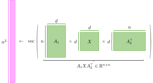
Figure 1: Left-hand side of the first equation in Claim 50. Given $A_{1},A_{2}\in\mathbb{R}^{n\times d}$ and $X\in\mathbb{R}^{d\times d}$. We turn $A_{1}XA_{2}^{\top}\in\mathbb{R}^{n\times n}$ into a length-$n^{2}$ vector. Green matrices represent the terms without any operations; purple vector represents the term after one operation.

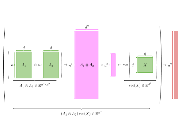
Figure 2: Right-hand side of the first equation in Claim 50. Given $A_{1},A_{2}\in\mathbb{R}^{n\times d}$ and $X\in\mathbb{R}^{d\times d}$. We first turn $A_{1},A_{2}\in\mathbb{R}^{n\times d}$ into a $n^{2}\times d^{2}$ matrix by Kronecker product and turn $X\in\mathbb{R}^{d\times d}$ into a $d^{2}$ dimensional vector by $\operatorname{vec}(\cdot)$. Then, we multiply $A_{1}\otimes A_{2}$ with $\operatorname{vec}(X)$ to get an $n^{2}$ dimensional vector. Green matrices represent the terms without any operations; purple vector/matrix represents the term after one operation; red vector represents the term after two operations.

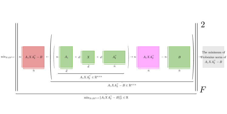
Figure 3: Left-hand side of the second equation in Claim 50. Given $A_{1},A_{2}\in\mathbb{R}^{n\times d}$, $X\in\mathbb{R}^{d\times d}$, and $B\in\mathbb{R}^{n\times n}$. We first find $A_{1}XA_{2}^{\top}\in\mathbb{R}^{n\times n}$. Then, we subtract $B\in\mathbb{R}^{n\times n}$ from $A_{1}XA_{2}^{\top}$. Finally, we compute the minimum of the Frobenius norm of $A_{1}XA_{2}^{\top}-B$. Green matrices represent the terms without any operations; purple matrix represents the term after one operation; red matrix represents the term after two operations; grey scalar represents the term after three operations.

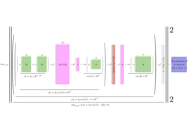
Figure 4: Right-hand side of the second equation in Claim 50. Given $A_{1},A_{2}\in\mathbb{R}^{n\times d}$, $X\in\mathbb{R}^{d\times d}$, and $B\in\mathbb{R}^{n\times n}$. We first turn $A_{1},A_{2}\in\mathbb{R}^{n\times d}$ into a $n^{2}\times d^{2}$ matrix by Kronecker product, turn $X\in\mathbb{R}^{d\times d}$ into a $d^{2}$ dimensional vector by $\operatorname{vec}(\cdot)$, and turn $B\in\mathbb{R}^{n\times n}$ into a $n^{2}$ dimensional vector by $\operatorname{vec}(\cdot)$, namely $b=\operatorname{vec}(B)$ and $x=\operatorname{vec}(X)$. Then, we multiply $A_{1}\otimes A_{2}$ with $\operatorname{vec}(X)$ to get an $n^{2}$ dimensional vector. After that, we subtract $\operatorname{vec}(B)$ from $(A_{1}\otimes A_{2})\operatorname{vec}(X)$. Finally, we compute the minimum of the $\ell_{2}$ norm of $(A_{1}\otimes A_{2})\operatorname{vec}(X)$. Green matrices represent the terms without any operations; purple vectors/matrix represent the term after one operation; red vector represents the term after two operations; gray vector represents the term after three operations; blue scalar represents the term after four operations.

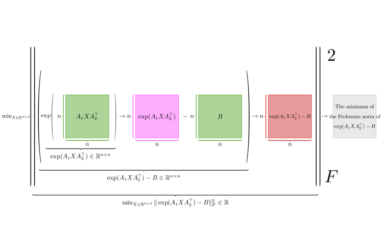
Figure 5: Left-hand side of the third equation in Claim 50. Given $A_{1}XA_{2}\in\mathbb{R}^{n\times n}$ and $B\in\mathbb{R}^{n\times n}$. We first find $\exp(A_{1}XA_{2}^{\top})\in\mathbb{R}^{n\times n}$. Then, we subtract $B\in\mathbb{R}^{n\times n}$ from $\exp(A_{1}XA_{2}^{\top})$. Finally, we compute the minimum of the Frobenius norm of $\exp(A_{1}XA_{2}^{\top})-B$. Green matrices represent the terms without any operations; purple matrix represents the term after one operation; red matrix represents the term after two operations; grey scalar represents the term after three operations.

Figure 6: Right-hand side of the third equation in Claim 50. Given $(A_{1}\otimes A_{2})x\in\mathbb{R}^{n^{2}}$ and $b\in\mathbb{R}^{n^{2}}$. We first find $\exp((A_{1}\otimes A_{2})x)\in\mathbb{R}^{n^{2}}$. Then, we subtract $b\in\mathbb{R}^{n^{2}}$ from $\exp((A_{1}\otimes A_{2})x)$. Finally, we compute the minimum of the $\ell_{2}$ norm of $\exp((A_{1}\otimes A_{2})x)-b$. Green vectors represent the terms without any operations; purple vector represents the term after one operation; red vector represents the term after two operations; grey scalar represents the term after three operations.

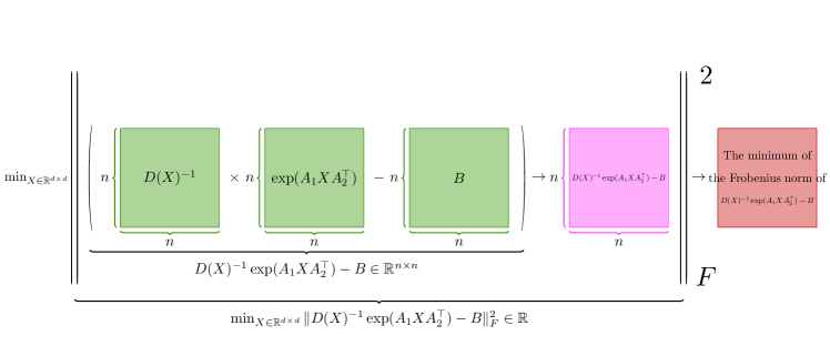
Figure 7: Left-hand side of the fourth equation in Claim 50. Given $\exp(A_{1}XA_{2}),B,D(X)^{-1}\in\mathbb{R}^{n\times n}$. We first find $D(X)^{-1}\exp(A_{1}XA_{2}^{\top})-B\in\mathbb{R}^{n\times n}$. Then, we compute the minimum of the Frobenius norm of $D(X)^{-1}\exp(A_{1}XA_{2}^{\top})-B$. Green matrices represent the terms without any operations; purple matrix represents the term after one operation; red scalar represents the term after two operations.

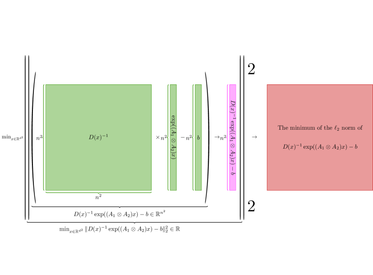
Figure 8: Right-hand side of the fourth equation in Claim 50. Given $\exp((A_{1}\otimes A_{2})x),b\in\mathbb{R}^{n^{2}}$ and $D(x)^{-1}\in\mathbb{R}^{n^{2}\times n^{2}}$. We first find $D(x)^{-1}\exp((A_{1}\otimes A_{2})x)-b\in\mathbb{R}^{n^{2}}$. Then, we compute the minimum of the $\ell_{2}$ norm of $D(x)^{-1}\exp((A_{1}\otimes A_{2})x)-b$. Green matrix/vectors represent the terms without any operations; purple vector represents the term after one operation; red scalar represents the term after two operations.

C.3 Basic Derivatives

Now, we compute the first-order derivatives. Similar calculations can be found in [40, 57].

Lemma 51.

If we have that

• $A_{1}$ and $A_{2}$ are two arbitrary matrices in $\mathbb{R}^{n\times d}$.

• $\mathsf{A}=A_{1}\otimes A_{2}$ (recall Definition 38).

• $X$ is an arbitrary matrix in $\mathbb{R}^{d\times d}$.

• $D(x)$ is defined in Definition 40.

• $x$ is an arbitrary vector in $\mathbb{R}^{d^{2}}$, satisfying $x=\operatorname{vec}(X)$.

Then, we can show

• Part 1. For each $i\in[d^{2}]$,

  $$\frac{\mathrm{d}\mathsf{A}x}{\mathrm{d}x_{i}}=\mathsf{A}_{*,i}$$

• Part 2. For each $i\in[d^{2}]$,

  $$\frac{\mathrm{d}\exp(\mathsf{A}x)}{\mathrm{d}x_{i}}=\exp(\mathsf{A}x)\circ\mathsf{A}_{*,i}$$

• Part 3. For each $j_{1}\in[n]$, for each $i\in[d^{2}]$,

  $$\frac{\mathrm{d}\mathsf{A}_{[j_{1}],*}x}{\mathrm{d}x_{i}}=\mathsf{A}_{[j_{1}],i}$$

• Part 4. For each $j_{1}\in[n]$, for each $i\in[d^{2}]$,

  $$\frac{\mathrm{d}u(x)_{j_{1}}}{\mathrm{d}x_{i}}=u(x)_{j_{1}}\circ\mathsf{A}_{[j_{1}],i}$$

• Part 5. For each $j_{1}\in[n]$, for each $i\in[d^{2}]$,

  $$\frac{\mathrm{d}\alpha(x)_{j_{1}}}{\mathrm{d}x}=\langle u(x)_{j_{1}},\mathsf{A}_{[j_{1}],i}\rangle$$

• Part 6. For each $j_{1}\in[n]$, for each $i\in[d^{2}]$,

  $$\frac{\mathrm{d}\alpha(x)_{i_{1}}^{-1}}{\mathrm{d}x_{i}}=-\alpha(x)_{j_{1}}^{-1}\cdot\langle f(x)_{j_{1}},\mathsf{A}_{[j_{1}],i}\rangle$$

• Part 7. For each $j_{1}\in[n]$, for each $i\in[d^{2}]$,

  $$\frac{\mathrm{d}f(x)_{j_{1}}}{\mathrm{d}x_{i}}=f(x)_{j_{1}}\circ\mathsf{A}_{[j_{1}],i}-f(x)_{j_{1}}\cdot\langle f(x)_{j_{1}},\mathsf{A}_{[j_{1}],i}\rangle.$$

• Part 8. For each $j_{1}\in[n]$, for each $i\in[d^{2}]$,

  $$\frac{\mathrm{d}c(x)_{j_{1}}}{\mathrm{d}x_{i}}=\frac{\mathrm{d}f(x)_{j_{1}}}{\mathrm{d}x_{i}}$$

• Part 9. For each $i\in[d^{2}]$,

  $$~{}\frac{\mathrm{d}L_{\exp}(x)}{\mathrm{d}x_{i}}$$

  $$= ~{}\sum_{j_{1}=1}^{n}(\langle c(x)_{j_{1}},f(x)_{j_{1}}\circ\mathsf{A}_{[j_{1}],i}\rangle-\langle c(x)_{j_{1}},f(x)_{j_{1}}\rangle\cdot\langle f(x)_{j_{1}},\mathsf{A}_{[j_{1}],i}\rangle).$$

Appendix D Hessian

In this section, our attention is directed towards the Hessian property inherent in our loss function. This investigation serves as a preparatory step for substantiating the convergence proof of our training procedure. While [40] outlines a singular version of a similar problem, we aim to showcase that our computations extend this scenario by a factor of $n$. Drawing upon the Hessian property expounded upon in [40], it becomes evident that our loss function similarly exhibits this particular property.

In Section D.1, we compute the second order derivative of $u(x)_{j_{1}}$. In Section D.2, we compute the second order derivative of $\alpha(x)_{j_{1}}$. In Section D.3, we compute the second order derivative of $\alpha(x)_{j_{1}}^{-1}$. In Section D.4, we compute the second order derivative of $f(x)_{j_{1}}$. In Section D.5, we compute the second order derivative of $L_{\exp}$. In Section D.6, we compute the hessian of a single loss. In Section D.7, we simplify the result that we get.

D.1 Second Order Derivatives of $u(x)_{j_{1}}$

In this section, we start to compute the second-order derivative of $u(x)_{j_{1}}$.

Lemma 52.

If the following conditions hold

• Let $u$ be defined as in Definition 42.

• Let $x\in\mathbb{R}^{d^{2}}$, satisfying $x=\operatorname{vec}(X)$.

• Let $A_{1},A_{2}\in\mathbb{R}^{n\times d}$.

• Let $\mathsf{A}=A_{1}\otimes A_{2}$.

Then, we have

• For each $i\in[d^{2}]$,

  $$\frac{\mathrm{d}^{2}u(x)_{j_{1}}}{\mathrm{d}x_{i}^{2}}=u(x)_{j_{1}}\circ\mathsf{A}_{[j_{1}],i}\circ\mathsf{A}_{[j_{1}],i}.$$

• For each $i\in[d^{2}],l\in[d^{2}]$

  $$\frac{\mathrm{d}^{2}u(x)_{j_{1}}}{\mathrm{d}x_{i}\mathrm{d}x_{l}}=u(x)_{j_{1}}\circ\mathsf{A}_{[j_{1}],l}\circ\mathsf{A}_{[j_{1}],i}.$$

Proof.

We have

$$\frac{\mathrm{d}^{2}u(x)_{j_{1}}}{\mathrm{d}x_{i}^{2}}= ~{}\frac{\mathrm{d}}{\mathrm{d}x_{i}}(\frac{\mathrm{d}u(x)_{j_{1}}}{\mathrm{d}x_{i}})$$

$$= ~{}\frac{\mathrm{d}(u(x)_{j_{1}}\circ\mathsf{A}_{[j_{1}],i})}{\mathrm{d}x_{i}}$$

$$= ~{}\frac{\mathrm{d}(u(x)_{j_{1}})}{\mathrm{d}x_{i}}\circ\mathsf{A}_{[j_{1}],i}+u(x)_{j_{1}}\circ\frac{\mathrm{d}(\mathsf{A}_{[j_{1}],i})}{\mathrm{d}x_{i}}$$

$$= ~{}u(x)_{j_{1}}\circ\mathsf{A}_{[j_{1}],i}\circ\mathsf{A}_{[j_{1}],i}$$

where the first step follows from simple algebra, the second step follows from Part 4 of Lemma 51, the third step follows from Fact 17, and the last step follows from Part 4 of Lemma 51 and $\frac{\mathrm{d}(\mathsf{A}_{[j_{1}],i})}{\mathrm{d}x_{i}}=0$.

Also, we can get

$$\frac{\mathrm{d}^{2}u(x)_{j_{1}}}{\mathrm{d}x_{i}\mathrm{d}x_{l}}= ~{}\frac{\mathrm{d}}{\mathrm{d}x_{l}}(\frac{\mathrm{d}u(x)_{j_{1}}}{\mathrm{d}x_{i}})$$

$$= ~{}\frac{\mathrm{d}(u(x)_{j_{1}}\circ\mathsf{A}_{[j_{1}],i})}{\mathrm{d}x_{l}}$$

$$= ~{}\frac{\mathrm{d}(u(x)_{j_{1}})}{\mathrm{d}x_{l}}\circ\mathsf{A}_{[j_{1}],i}+u(x)_{j_{1}}\circ\frac{\mathrm{d}(\mathsf{A}_{[j_{1}],i})}{\mathrm{d}x_{l}}$$

$$= ~{}u(x)_{j_{1}}\circ\mathsf{A}_{[j_{1}],l}\circ\mathsf{A}_{[j_{1}],i}$$

where the first step follows from simple algebra, the second step follows from Part 4 of Lemma 51, the third step follows from Fact 17, and the last step follows from Part 4 of Lemma 51 and $\frac{\mathrm{d}(\mathsf{A}_{[j_{1}],i})}{\mathrm{d}x_{i}}=0$. ∎

D.2 Second Order Derivatives of $\alpha(x)_{j_{1}}$

In this section, we start to compute the second-order derivative of $\alpha(x)_{j_{1}}$.

Lemma 53.

If the following conditions hold

• Let $\alpha$ be defined as in Definition 41.

• Let $x\in\mathbb{R}^{d^{2}}$, satisfying $x=\operatorname{vec}(X)$.

• Let $A_{1},A_{2}\in\mathbb{R}^{n\times d}$.

• Let $\mathsf{A}=A_{1}\otimes A_{2}$.

Then, we have

• For each $i\in[d^{2}]$,

  $$\frac{\mathrm{d}^{2}\alpha(x)_{j_{1}}}{\mathrm{d}x_{i}^{2}}=\langle u(x)_{j_{1}},\mathsf{A}_{[j_{1}],i}^{2}\rangle.$$

• For each $i,l\in[d^{2}]$,

  $$\frac{\mathrm{d}^{2}\alpha(x)_{j_{1}}}{\mathrm{d}x_{i}\mathrm{d}x_{l}}=\langle u(x)_{j_{1}},\mathsf{A}_{[j_{1}],i}\circ\mathsf{A}_{[j_{1}],l}\rangle.$$

Proof.

We have

$$\frac{\mathrm{d}^{2}\alpha(x)_{j_{1}}}{\mathrm{d}x_{i}^{2}}= ~{}\frac{\mathrm{d}}{\mathrm{d}x_{i}}(\frac{\mathrm{d}\alpha(x)_{j_{1}}}{\mathrm{d}x_{i}})$$

$$= ~{}\frac{\mathrm{d}(\langle u(x)_{j_{1}},\mathsf{A}_{[j_{1}],i}\rangle)}{\mathrm{d}x_{i}}$$

$$= ~{}\langle\frac{\mathrm{d}u(x)_{j_{1}}}{\mathrm{d}x_{i}},\mathsf{A}_{[j_{1}],i}\rangle+\langle u(x)_{j_{1}},\frac{\mathrm{d}\mathsf{A}_{[j_{1}],i}}{\mathrm{d}x_{i}}\rangle$$

$$= ~{}\langle u(x)_{j_{1}}\circ\mathsf{A}_{[j_{1}],i},\mathsf{A}_{[j_{1}],i}\rangle$$

$$= ~{}\langle u(x)_{j_{1}},\mathsf{A}_{[j_{1}],i}^{2}\rangle,$$

where the first step follows from simple algebra, the second step follows from Part 5 of Lemma 51, the third step follows from the definition of the inner product, the fourth step follows from $\frac{\mathrm{d}\mathsf{A}_{[j_{1}],i}}{\mathrm{d}x_{i}}=0$, and the last step follows from Fact 16.

Also, we can get

$$\frac{\mathrm{d}^{2}\alpha(x)_{j_{1}}}{\mathrm{d}x_{i}\mathrm{d}x_{l}}= ~{}\frac{\mathrm{d}}{\mathrm{d}x_{l}}(\frac{\mathrm{d}\alpha(x)_{j_{1}}}{\mathrm{d}x_{i}})$$

$$= ~{}\frac{\mathrm{d}(\langle u(x)_{j_{1}},\mathsf{A}_{[j_{1}],i}\rangle)}{\mathrm{d}x_{l}}$$

$$= ~{}\langle\frac{\mathrm{d}u(x)_{j_{1}}}{\mathrm{d}x_{l}},\mathsf{A}_{[j_{1}],i}\rangle+\langle u(x)_{j_{1}},\frac{\mathrm{d}\mathsf{A}_{[j_{1}],i}}{\mathrm{d}x_{l}}\rangle$$

$$= ~{}\langle u(x)_{j_{1}}\circ\mathsf{A}_{[j_{1}],l},\mathsf{A}_{[j_{1}],i}\rangle$$

$$= ~{}\langle u(x)_{j_{1}},\mathsf{A}_{[j_{1}],i}\circ\mathsf{A}_{[j_{1}],l}\rangle,$$

where the first step follows from simple algebra, the second step follows from Part 5 of Lemma 51, the third step follows from the definition of the inner product, the fourth step follows from $\frac{\mathrm{d}\mathsf{A}_{[j_{1}],i}}{\mathrm{d}x_{i}}=0$, and the last step follows from Fact 16. ∎

D.3 Second Order Derivatives of $\alpha(x)_{j_{1}}^{-1}$

In this section, we start to compute the second-order derivative of $\alpha(x)_{j_{1}}^{-1}$.

Lemma 54.

If the following conditions hold

• Let $\alpha$ be defined as in Definition 41.

• Let $f$ be defined as in Definition 43.

• Let $x\in\mathbb{R}^{d^{2}}$, satisfying $x=\operatorname{vec}(X)$.

• Let $A_{1},A_{2}\in\mathbb{R}^{n\times d}$.

• Let $\mathsf{A}=A_{1}\otimes A_{2}$.

Then, we have

• For each $i\in[d^{2}]$,

  $$\frac{\mathrm{d}^{2}\alpha(x)_{j_{1}}^{-1}}{\mathrm{d}x_{i}^{2}}=2\alpha(x)_{j_{1}}^{-1}\cdot\langle f(x)_{j_{1}},\mathsf{A}_{[j_{1}],i}\rangle^{2}-\alpha(x)_{j_{1}}^{-1}\cdot\langle f(x)_{j_{1}},\mathsf{A}_{[j_{1}],i}^{2}\rangle.$$

• For each $i,l\in[d^{2}]$,

  $$\frac{\mathrm{d}^{2}\alpha(x)_{j_{1}}^{-1}}{\mathrm{d}x_{i}\mathrm{d}x_{l}}=2\alpha(x)_{j_{1}}^{-1}\cdot\langle f(x)_{j_{1}},\mathsf{A}_{[j_{1}],l}\rangle\cdot\langle f(x)_{j_{1}},\mathsf{A}_{[j_{1}],i}\rangle-\alpha(x)_{j_{1}}^{-1}\cdot\langle f(x)_{j_{1}},\mathsf{A}_{[j_{1}],i}\circ\mathsf{A}_{[j_{1}],l}\rangle.$$

Proof.

We have

$$\frac{\mathrm{d}^{2}\alpha(x)_{j_{1}}^{-1}}{\mathrm{d}x_{i}^{2}}= ~{}\frac{\mathrm{d}}{\mathrm{d}x_{i}}(\frac{\mathrm{d}\alpha(x)_{j_{1}}^{-1}}{\mathrm{d}x_{i}})$$

$$= ~{}\frac{\mathrm{d}(-\alpha(x)_{j_{1}}^{-1}\cdot\langle f(x)_{j_{1}},\mathsf{A}_{[j_{1}],i}\rangle)}{\mathrm{d}x_{i}}$$

$$= ~{}\frac{\mathrm{d}(-\alpha(x)_{j_{1}}^{-1})}{\mathrm{d}x_{i}}\cdot\langle f(x)_{j_{1}},\mathsf{A}_{[j_{1}],i}\rangle+(-\alpha(x)_{j_{1}}^{-1})\cdot\frac{\mathrm{d}\langle f(x)_{j_{1}},\mathsf{A}_{[j_{1}],i}\rangle}{\mathrm{d}x_{i}}$$

$$= ~{}\alpha(x)_{j_{1}}^{-1}\cdot\langle f(x)_{j_{1}},\mathsf{A}_{[j_{1}],i}\rangle^{2}+(-\alpha(x)_{j_{1}}^{-1})\cdot\frac{\mathrm{d}\langle f(x)_{j_{1}},\mathsf{A}_{[j_{1}],i}\rangle}{\mathrm{d}x_{i}},$$ (1)

where the first step follows from simple algebra, the second step follows from Part 6 of Lemma 51, the third step follows from Fact 17, and the last step follows from Part 6 of Lemma 51.

To compute the second term of Eq. (D.3), we have

$$\frac{\mathrm{d}\langle f(x)_{j_{1}},\mathsf{A}_{[j_{1}],i}\rangle}{\mathrm{d}x_{i}}= ~{}\langle\frac{\mathrm{d}f(x)_{j_{1}}}{\mathrm{d}x_{i}},\mathsf{A}_{[j_{1}],i}\rangle$$

$$= ~{}\langle f(x)_{j_{1}}\circ\mathsf{A}_{[j_{1}],i}-f(x)_{j_{1}}\cdot\langle f(x)_{j_{1}},\mathsf{A}_{[j_{1}],i}\rangle,\mathsf{A}_{[j_{1}],i}\rangle$$

$$= ~{}\langle f(x)_{j_{1}}\circ\mathsf{A}_{[j_{1}],i},\mathsf{A}_{[j_{1}],i}\rangle-\langle f(x)_{j_{1}}\cdot\langle f(x)_{j_{1}},\mathsf{A}_{[j_{1}],i}\rangle,\mathsf{A}_{[j_{1}],i}\rangle$$

$$= ~{}\langle f(x)_{j_{1}},\mathsf{A}_{[j_{1}],i}^{2}\rangle-\langle f(x)_{j_{1}},\mathsf{A}_{[j_{1}],i}\rangle^{2},$$ (2)

where the first step follows from the definition of the inner product, the second step follows from Part 7 of Lemma 51 and $\frac{\mathrm{d}\mathsf{A}_{[j_{1}],i}}{\mathrm{d}x_{i}}=0$, the third step follows from Fact 16, and the last step follows from Fact 16.

Combining Eq. (D.3) and Eq. (D.3), we have

$$\frac{\mathrm{d}^{2}\alpha(x)_{j_{1}}^{-1}}{\mathrm{d}x_{i}^{2}}= ~{}\alpha(x)_{j_{1}}^{-1}\cdot\langle f(x)_{j_{1}},\mathsf{A}_{[j_{1}],i}\rangle^{2}-\alpha(x)_{j_{1}}^{-1}\cdot(\langle f(x)_{j_{1}},\mathsf{A}_{[j_{1}],i}^{2}\rangle-\langle f(x)_{j_{1}},\mathsf{A}_{[j_{1}],i}\rangle^{2})$$

$$= ~{}\alpha(x)_{j_{1}}^{-1}\cdot\langle f(x)_{j_{1}},\mathsf{A}_{[j_{1}],i}\rangle^{2}-\alpha(x)_{j_{1}}^{-1}\cdot\langle f(x)_{j_{1}},\mathsf{A}_{[j_{1}],i}^{2}\rangle+\alpha(x)_{j_{1}}^{-1}\cdot\langle f(x)_{j_{1}},\mathsf{A}_{[j_{1}],i}\rangle^{2}$$

$$= ~{}2\alpha(x)_{j_{1}}^{-1}\cdot\langle f(x)_{j_{1}},\mathsf{A}_{[j_{1}],i}\rangle^{2}-\alpha(x)_{j_{1}}^{-1}\cdot\langle f(x)_{j_{1}},\mathsf{A}_{[j_{1}],i}^{2}\rangle,$$

where the second and the third step both follow from simple algebra.

Then, to compute $\frac{\mathrm{d}^{2}\alpha(x)_{j_{1}}^{-1}}{\mathrm{d}x_{i}\mathrm{d}x_{l}}$, we have

$$\frac{\mathrm{d}^{2}\alpha(x)_{j_{1}}^{-1}}{\mathrm{d}x_{i}\mathrm{d}x_{l}}= ~{}\frac{\mathrm{d}}{\mathrm{d}x_{l}}(\frac{\mathrm{d}\alpha(x)_{j_{1}}^{-1}}{\mathrm{d}x_{i}})$$

$$= ~{}\frac{\mathrm{d}(-\alpha(x)_{j_{1}}^{-1}\cdot\langle f(x)_{j_{1}},\mathsf{A}_{[j_{1}],i}\rangle)}{\mathrm{d}x_{l}}$$

$$= ~{}\frac{\mathrm{d}(-\alpha(x)_{j_{1}}^{-1})}{\mathrm{d}x_{l}}\cdot\langle f(x)_{j_{1}},\mathsf{A}_{[j_{1}],i}\rangle+(-\alpha(x)_{j_{1}}^{-1})\cdot\frac{\mathrm{d}\langle f(x)_{j_{1}},\mathsf{A}_{[j_{1}],i}\rangle}{\mathrm{d}x_{l}}$$

$$= ~{}\alpha(x)_{j_{1}}^{-1}\cdot\langle f(x)_{j_{1}},\mathsf{A}_{[j_{1}],l}\rangle\cdot\langle f(x)_{j_{1}},\mathsf{A}_{[j_{1}],i}\rangle-\alpha(x)_{j_{1}}^{-1}\cdot\frac{\mathrm{d}\langle f(x)_{j_{1}},\mathsf{A}_{[j_{1}],i}\rangle}{\mathrm{d}x_{l}},$$ (3)

where the first step follows from simple algebra, the second step follows from Part 6 of Lemma 51, the third step follows from Fact 17, and the last step follows from Part 6 of Lemma 51.

To compute the second term of Eq. (D.3), we have

$$\frac{\mathrm{d}\langle f(x)_{j_{1}},\mathsf{A}_{[j_{1}],i}\rangle}{\mathrm{d}x_{l}}= ~{}\langle\frac{\mathrm{d}f(x)_{j_{1}}}{\mathrm{d}x_{l}},\mathsf{A}_{[j_{1}],i}\rangle+\langle f(x)_{j_{1}},\frac{\mathrm{d}\mathsf{A}_{[j_{1}],i}}{\mathrm{d}x_{l}}\rangle$$

$$= ~{}\langle f(x)_{j_{1}}\circ\mathsf{A}_{[j_{1}],l}-f(x)_{j_{1}}\cdot\langle f(x)_{j_{1}},\mathsf{A}_{[j_{1}],l}\rangle,\mathsf{A}_{[j_{1}],i}\rangle$$

$$= ~{}\langle f(x)_{j_{1}}\circ\mathsf{A}_{[j_{1}],l},\mathsf{A}_{[j_{1}],i}\rangle-\langle f(x)_{j_{1}}\cdot\langle f(x)_{j_{1}},\mathsf{A}_{[j_{1}],l}\rangle,\mathsf{A}_{[j_{1}],i}\rangle$$

$$= ~{}\langle f(x)_{j_{1}},\mathsf{A}_{[j_{1}],i}\circ\mathsf{A}_{[j_{1}],l}\rangle-\langle f(x)_{j_{1}},\mathsf{A}_{[j_{1}],l}\rangle\cdot\langle f(x)_{j_{1}},\mathsf{A}_{[j_{1}],i}\rangle,$$ (4)

where the first step follows from the definition of the inner product, the second step follows from Part 7 of Lemma 51 and $\frac{\mathrm{d}\mathsf{A}_{[j_{1}],i}}{\mathrm{d}x_{l}}=0$, the third step follows from Fact 16, and the last step follows from Fact 16.

By simple algebra, we can combine Eq. (D.3) and Eq. (D.3) as:

$$\frac{\mathrm{d}^{2}\alpha(x)_{j_{1}}^{-1}}{\mathrm{d}x_{i}\mathrm{d}x_{l}}=2\alpha(x)_{j_{1}}^{-1}\cdot\langle f(x)_{j_{1}},\mathsf{A}_{[j_{1}],l}\rangle\cdot\langle f(x)_{j_{1}},\mathsf{A}_{[j_{1}],i}\rangle-\alpha(x)_{j_{1}}^{-1}\cdot\langle f(x)_{j_{1}},\mathsf{A}_{[j_{1}],i}\circ\mathsf{A}_{[j_{1}],l}\rangle.$$

∎

D.4 Second Order Derivatives of $f(x)_{j_{1}}$

In this section, we start to compute the second-order derivative of $f(x)_{j_{1}}$.

Lemma 55.

If the following conditions hold

• Let $f$ be defined as in Definition 43.

• Let $x\in\mathbb{R}^{d^{2}}$, satisfying $x=\operatorname{vec}(X)$.

• Let $A_{1},A_{2}\in\mathbb{R}^{n\times d}$.

• Let $\mathsf{A}=A_{1}\otimes A_{2}$.

Then, we have

• For each $i\in[d^{2}]$,

  $$\frac{\mathrm{d}^{2}f(x)_{j_{1}}}{\mathrm{d}x_{i}^{2}}= ~{}f(x)_{j_{1}}\circ\mathsf{A}_{[j_{1}],i}^{2}-2f(x)_{j_{1}}\circ\mathsf{A}_{[j_{1}],i}\cdot\langle f(x)_{j_{1}},\mathsf{A}_{[j_{1}],i}\rangle$$

  $$~{}-f(x)_{j_{1}}\cdot\langle f(x)_{j_{1}},\mathsf{A}_{[j_{1}],i}^{2}\rangle+2f(x)_{j_{1}}\cdot\langle f(x)_{j_{1}},\mathsf{A}_{[j_{1}],i}\rangle^{2}.$$

• For each $i,l\in[d^{2}]$,

  $$\frac{\mathrm{d}^{2}f(x)_{j_{1}}}{\mathrm{d}x_{i}\mathrm{d}x_{l}}= ~{}f(x)_{j_{1}}\circ\mathsf{A}_{[j_{1}],i}\circ\mathsf{A}_{[j_{1}],l}-f(x)_{j_{1}}\circ\mathsf{A}_{[j_{1}],i}\cdot\langle f(x)_{j_{1}},\mathsf{A}_{[j_{1}],l}\rangle$$

  $$~{}-f(x)_{j_{1}}\circ\mathsf{A}_{[j_{1}],l}\cdot\langle f(x)_{j_{1}},\mathsf{A}_{[j_{1}],i}\rangle+2f(x)_{j_{1}}\cdot\langle f(x)_{j_{1}},\mathsf{A}_{[j_{1}],i}\rangle\cdot\langle f(x)_{j_{1}},\mathsf{A}_{[j_{1}],l}\rangle$$

  $$~{}-f(x)_{j_{1}}\cdot\langle f(x)_{j_{1}},\mathsf{A}_{[j_{1}],i}\circ\mathsf{A}_{[j_{1}],l}\rangle.$$

Proof.

We first consider $\frac{\mathrm{d}^{2}f(x)_{j_{1}}}{\mathrm{d}x_{i}^{2}}$.

We have

$$\frac{\mathrm{d}^{2}f(x)_{j_{1}}}{\mathrm{d}x_{i}^{2}}= ~{}\frac{\mathrm{d}}{\mathrm{d}x_{i}}(\frac{\mathrm{d}f(x)_{j_{1}}}{\mathrm{d}x_{i}})$$

$$= ~{}\frac{\mathrm{d}(f(x)_{j_{1}}\circ\mathsf{A}_{[j_{1}],i}-f(x)_{j_{1}}\cdot\langle f(x)_{j_{1}},\mathsf{A}_{[j_{1}],i}\rangle)}{\mathrm{d}x_{i}}$$

$$= ~{}\frac{\mathrm{d}f(x)_{j_{1}}\circ\mathsf{A}_{[j_{1}],i}}{\mathrm{d}x_{i}}-\frac{\mathrm{d}f(x)_{j_{1}}\cdot\langle f(x)_{j_{1}},\mathsf{A}_{[j_{1}],i}\rangle}{\mathrm{d}x_{i}},$$ (5)

where the first step follows from simple algebra, the second step is due to Fact 17, and the third step is based on Fact 17.

To compute the first term of Eq. (D.4), we have

$$\frac{\mathrm{d}f(x)_{j_{1}}\circ\mathsf{A}_{[j_{1}],i}}{\mathrm{d}x_{i}}= ~{}f(x)_{j_{1}}\circ\frac{\mathrm{d}\mathsf{A}_{[j_{1}],i}}{\mathrm{d}x_{i}}+\frac{\mathrm{d}f(x)_{j_{1}}}{\mathrm{d}x_{i}}\circ\mathsf{A}_{[j_{1}],i}$$

$$= ~{}(f(x)_{j_{1}}\circ\mathsf{A}_{[j_{1}],i}-f(x)_{j_{1}}\cdot\langle f(x)_{j_{1}},\mathsf{A}_{[j_{1}],i}\rangle)\circ\mathsf{A}_{[j_{1}],i}$$

$$= ~{}f(x)_{j_{1}}\circ\mathsf{A}_{[j_{1}],i}^{2}-f(x)_{j_{1}}\circ\mathsf{A}_{[j_{1}],i}\cdot\langle f(x)_{j_{1}},\mathsf{A}_{[j_{1}],i}\rangle,$$ (6)

where the first step follows from Fact 17, the second step follows from $\frac{\mathrm{d}\mathsf{A}_{[j_{1}],i}}{\mathrm{d}x_{i}}=0$ and Part 7 of Lemma 51, and the last step follows from the property of Hadamard product.

To compute the second term of Eq. (D.4), we have

$$\frac{\mathrm{d}f(x)_{j_{1}}\cdot\langle f(x)_{j_{1}},\mathsf{A}_{[j_{1}],i}\rangle}{\mathrm{d}x_{i}}= ~{}\frac{\mathrm{d}f(x)_{j_{1}}}{\mathrm{d}x_{i}}\cdot\langle f(x)_{j_{1}},\mathsf{A}_{[j_{1}],i}\rangle+f(x)_{j_{1}}\cdot\frac{\mathrm{d}\langle f(x)_{j_{1}},\mathsf{A}_{[j_{1}],i}\rangle}{\mathrm{d}x_{i}}$$

$$= ~{}(f(x)_{j_{1}}\circ\mathsf{A}_{[j_{1}],i}-f(x)_{j_{1}}\cdot\langle f(x)_{j_{1}},\mathsf{A}_{[j_{1}],i}\rangle)\cdot\langle f(x)_{j_{1}},\mathsf{A}_{[j_{1}],i}\rangle$$

$$~{}+f(x)_{j_{1}}\cdot\frac{\mathrm{d}\langle f(x)_{j_{1}},\mathsf{A}_{[j_{1}],i}\rangle}{\mathrm{d}x_{i}}$$

$$= ~{}(f(x)_{j_{1}}\circ\mathsf{A}_{[j_{1}],i}-f(x)_{j_{1}}\cdot\langle f(x)_{j_{1}},\mathsf{A}_{[j_{1}],i}\rangle)\cdot\langle f(x)_{j_{1}},\mathsf{A}_{[j_{1}],i}\rangle$$

$$~{}+f(x)_{j_{1}}\cdot(\langle f(x)_{j_{1}},\mathsf{A}_{[j_{1}],i}^{2}\rangle-\langle f(x)_{j_{1}},\mathsf{A}_{[j_{1}],i}\rangle^{2})$$

$$= ~{}f(x)_{j_{1}}\circ\mathsf{A}_{[j_{1}],i}\cdot\langle f(x)_{j_{1}},\mathsf{A}_{[j_{1}],i}\rangle-f(x)_{j_{1}}\cdot\langle f(x)_{j_{1}},\mathsf{A}_{[j_{1}],i}\rangle^{2}$$

$$~{}+f(x)_{j_{1}}\cdot\langle f(x)_{j_{1}},\mathsf{A}_{[j_{1}],i}^{2}\rangle-f(x)_{j_{1}}\cdot\langle f(x)_{j_{1}},\mathsf{A}_{[j_{1}],i}\rangle^{2}$$

$$= ~{}f(x)_{j_{1}}\circ\mathsf{A}_{[j_{1}],i}\cdot\langle f(x)_{j_{1}},\mathsf{A}_{[j_{1}],i}\rangle+f(x)_{j_{1}}\cdot\langle f(x)_{j_{1}},\mathsf{A}_{[j_{1}],i}^{2}\rangle$$

$$~{}-2f(x)_{j_{1}}\cdot\langle f(x)_{j_{1}},\mathsf{A}_{[j_{1}],i}\rangle^{2},$$ (7)

where the first step follows from Fact 17, the second step follows from Part 7 of Lemma 51, the third step follows from the proof of Lemma 54 (see Eq. (D.3)), and the fourth and the fifth step follows from simple algebra.

Combining Eq. (D.4), Eq. (D.4), and Eq. (D.4), we have

$$\frac{\mathrm{d}^{2}f(x)_{j_{1}}}{\mathrm{d}x_{i}^{2}}= ~{}f(x)_{j_{1}}\circ\mathsf{A}_{[j_{1}],i}^{2}-2f(x)_{j_{1}}\circ\mathsf{A}_{[j_{1}],i}\cdot\langle f(x)_{j_{1}},\mathsf{A}_{[j_{1}],i}\rangle$$

$$~{}-f(x)_{j_{1}}\cdot\langle f(x)_{j_{1}},\mathsf{A}_{[j_{1}],i}^{2}\rangle+2f(x)_{j_{1}}\cdot\langle f(x)_{j_{1}},\mathsf{A}_{[j_{1}],i}\rangle^{2}.$$

Now, we consider $\frac{\mathrm{d}^{2}f(x)_{j_{1}}}{\mathrm{d}x_{i}\mathrm{d}x_{l}}$.

We have

$$\frac{\mathrm{d}^{2}f(x)_{j_{1}}}{\mathrm{d}x_{i}\mathrm{d}x_{l}}= ~{}\frac{\mathrm{d}}{\mathrm{d}x_{l}}(\frac{\mathrm{d}f(x)_{j_{1}}}{\mathrm{d}x_{i}})$$

$$= ~{}\frac{\mathrm{d}(f(x)_{j_{1}}\circ\mathsf{A}_{[j_{1}],i}-f(x)_{j_{1}}\cdot\langle f(x)_{j_{1}},\mathsf{A}_{[j_{1}],i}\rangle)}{\mathrm{d}x_{l}}$$

$$= ~{}\frac{\mathrm{d}f(x)_{j_{1}}\circ\mathsf{A}_{[j_{1}],i}}{\mathrm{d}x_{l}}-\frac{\mathrm{d}f(x)_{j_{1}}\cdot\langle f(x)_{j_{1}},\mathsf{A}_{[j_{1}],i}\rangle}{\mathrm{d}x_{l}},$$ (8)

where the first step follows from simple algebra, the second step follows from Part 7 of Lemma 51, and the third step follows from Fact 17.

To compute the first term of Eq. (D.4), we have

$$\frac{\mathrm{d}f(x)_{j_{1}}\circ\mathsf{A}_{[j_{1}],i}}{\mathrm{d}x_{l}}= ~{}f(x)_{j_{1}}\circ\frac{\mathrm{d}\mathsf{A}_{[j_{1}],i}}{\mathrm{d}x_{l}}+\frac{\mathrm{d}f(x)_{j_{1}}}{\mathrm{d}x_{l}}\circ\mathsf{A}_{[j_{1}],i}$$

$$= ~{}(f(x)_{j_{1}}\circ\mathsf{A}_{[j_{1}],l}-f(x)_{j_{1}}\cdot\langle f(x)_{j_{1}},\mathsf{A}_{[j_{1}],l}\rangle)\circ\mathsf{A}_{[j_{1}],i}$$

$$= ~{}f(x)_{j_{1}}\circ\mathsf{A}_{[j_{1}],i}\circ\mathsf{A}_{[j_{1}],l}-f(x)_{j_{1}}\circ\mathsf{A}_{[j_{1}],i}\cdot\langle f(x)_{j_{1}},\mathsf{A}_{[j_{1}],l}\rangle,$$ (9)

where the first step follows from Fact 17, the second step follows from $\frac{\mathrm{d}\mathsf{A}_{[j_{1}],i}}{\mathrm{d}x_{l}}=0$ and Part 7 of Lemma 51, the third step follows from the property of Hadamard product.

To compute the second term of Eq. (D.4), we have

$$\frac{\mathrm{d}f(x)_{j_{1}}\cdot\langle f(x)_{j_{1}},\mathsf{A}_{[j_{1}],i}\rangle}{\mathrm{d}x_{l}}= ~{}\frac{\mathrm{d}f(x)_{j_{1}}}{\mathrm{d}x_{l}}\cdot\langle f(x)_{j_{1}},\mathsf{A}_{[j_{1}],i}\rangle+f(x)_{j_{1}}\cdot\frac{\mathrm{d}\langle f(x)_{j_{1}},\mathsf{A}_{[j_{1}],i}\rangle}{\mathrm{d}x_{l}}$$

$$= ~{}(f(x)_{j_{1}}\circ\mathsf{A}_{[j_{1}],l}-f(x)_{j_{1}}\cdot\langle f(x)_{j_{1}},\mathsf{A}_{[j_{1}],l}\rangle)\cdot\langle f(x)_{j_{1}},\mathsf{A}_{[j_{1}],i}\rangle$$

$$~{}+f(x)_{j_{1}}\cdot\frac{\mathrm{d}\langle f(x)_{j_{1}},\mathsf{A}_{[j_{1}],i}\rangle}{\mathrm{d}x_{l}}$$

$$= ~{}(f(x)_{j_{1}}\circ\mathsf{A}_{[j_{1}],l}-f(x)_{j_{1}}\cdot\langle f(x)_{j_{1}},\mathsf{A}_{[j_{1}],l}\rangle)\cdot\langle f(x)_{j_{1}},\mathsf{A}_{[j_{1}],i}\rangle$$

$$~{}+f(x)_{j_{1}}\cdot(\langle f(x)_{j_{1}},\mathsf{A}_{[j_{1}],i}\circ\mathsf{A}_{[j_{1}],l}\rangle-\langle f(x)_{j_{1}},\mathsf{A}_{[j_{1}],l}\rangle\cdot\langle f(x)_{j_{1}},\mathsf{A}_{[j_{1}],i}\rangle)$$

$$= ~{}f(x)_{j_{1}}\circ\mathsf{A}_{[j_{1}],l}\cdot\langle f(x)_{j_{1}},\mathsf{A}_{[j_{1}],i}\rangle-f(x)_{j_{1}}\cdot\langle f(x)_{j_{1}},\mathsf{A}_{[j_{1}],i}\rangle\cdot\langle f(x)_{j_{1}},\mathsf{A}_{[j_{1}],l}\rangle$$

$$~{}+f(x)_{j_{1}}\cdot\langle f(x)_{j_{1}},\mathsf{A}_{[j_{1}],i}\circ\mathsf{A}_{[j_{1}],l}\rangle$$

$$~{}-f(x)_{j_{1}}\cdot\langle f(x)_{j_{1}},\mathsf{A}_{[j_{1}],l}\rangle\cdot\langle f(x)_{j_{1}},\mathsf{A}_{[j_{1}],i}\rangle,$$ (10)

where the first step follows from Fact 17, the second step follows from Part 7 of Lemma 51, the third step follows from the proof of Lemma 54 (see Eq. (D.3)), and the fourth and the fifth step follows from simple algebra.

Combining Eq. (D.4), Eq. (D.4), and Eq. (D.4), we have

$$\frac{\mathrm{d}^{2}f(x)_{j_{1}}}{\mathrm{d}x_{i}\mathrm{d}x_{l}}= ~{}f(x)_{j_{1}}\circ\mathsf{A}_{[j_{1}],i}\circ\mathsf{A}_{[j_{1}],l}-f(x)_{j_{1}}\circ\mathsf{A}_{[j_{1}],i}\cdot\langle f(x)_{j_{1}},\mathsf{A}_{[j_{1}],l}\rangle-f(x)_{j_{1}}\circ\mathsf{A}_{[j_{1}],l}\cdot\langle f(x)_{j_{1}},\mathsf{A}_{[j_{1}],i}\rangle$$

$$~{}+2f(x)_{j_{1}}\cdot\langle f(x)_{j_{1}},\mathsf{A}_{[j_{1}],i}\rangle\cdot\langle f(x)_{j_{1}},\mathsf{A}_{[j_{1}],l}\rangle-f(x)_{j_{1}}\cdot\langle f(x)_{j_{1}},\mathsf{A}_{[j_{1}],i}\circ\mathsf{A}_{[j_{1}],l}\rangle.$$

∎

D.5 Second Order Derivatives of $L_{\exp}$

In this section, we start to compute the second-order derivative of $L_{\exp}$.

Lemma 56.

If the following conditions hold

• Let $L_{\exp}$ be defined as in Definition 45.

• Let $f$ be defined as in Definition 43.

• Let $c$ be defined as in Definition 44.

• Let $x\in\mathbb{R}^{d^{2}}$, satisfying $x=\operatorname{vec}(X)$.

• Let $A_{1},A_{2}\in\mathbb{R}^{n\times d}$.

• Let $\mathsf{A}=A_{1}\otimes A_{2}$.

Then, we have

• For each $i\in[d^{2}]$,

  $$\frac{\mathrm{d}^{2}L_{\exp}}{\mathrm{d}x_{i}^{2}}= ~{}\sum_{j_{1}=1}^{n}(\|f(x)_{j_{1}}\circ\mathsf{A}_{[j_{1}],i}\|_{2}^{2}-\langle f(x)_{j_{1}},\mathsf{A}_{[j_{1}],i}\rangle\cdot\langle f(x)_{j_{1}}^{2},\mathsf{A}_{[j_{1}],i}\rangle$$

  $$~{}~{}~{}+\langle c(x)_{j_{1}},f(x)_{j_{1}}\circ\mathsf{A}_{[j_{1}],l}^{2}\rangle-\langle c(x)_{j_{1}},f(x)_{j_{1}}\circ\mathsf{A}_{[j_{1}],i}\rangle\cdot\langle f(x)_{j_{1}},\mathsf{A}_{[j_{1}],i}\rangle)$$

  $$~{}-\sum_{j_{1}=1}^{n}(\langle f(x)_{j_{1}}+c(x)_{j_{1}},f(x)_{j_{1}}\circ\mathsf{A}_{[j_{1}],i}\rangle\cdot\langle f(x)_{j_{1}},\mathsf{A}_{[j_{1}],i}\rangle$$

  $$~{}~{}~{}-\langle f(x)_{j_{1}}+c(x)_{j_{1}},f(x)_{j_{1}}\rangle\cdot\langle f(x)_{j_{1}},\mathsf{A}_{[j_{1}],i}\rangle^{2})$$

  $$~{}-\sum_{j_{1}=1}^{n}(\langle c(x)_{j_{1}},f(x)_{j_{1}}\rangle\cdot\langle f(x)_{j_{1}},\mathsf{A}_{[j_{1}],i}^{2}\rangle$$

  $$~{}~{}~{}-\langle c(x)_{j_{1}},f(x)_{j_{1}}\rangle\cdot\langle f(x)_{j_{1}},\mathsf{A}_{[j_{1}],i}\rangle^{2}),$$

• For each $i,l\in[d^{2}]$,

  $$\frac{\mathrm{d}^{2}L_{\exp}}{\mathrm{d}x_{i}\mathrm{d}x_{l}}= ~{}\sum_{j_{1}=1}^{n}(\langle f(x)_{j_{1}}\circ\mathsf{A}_{[j_{1}],l},f(x)_{j_{1}}\circ\mathsf{A}_{[j_{1}],i}\rangle-\langle f(x)_{j_{1}},f(x)_{j_{1}}\circ\mathsf{A}_{[j_{1}],i}\rangle\cdot\langle f(x)_{j_{1}},\mathsf{A}_{[j_{1}],l}\rangle$$

  $$~{}+\langle c(x)_{j_{1}},f(x)_{j_{1}}\circ\mathsf{A}_{[j_{1}],i}\circ\mathsf{A}_{[j_{1}],l}\rangle+\langle c(x)_{j_{1}},f(x)_{j_{1}}\circ\mathsf{A}_{[j_{1}],i}\rangle\cdot\langle f(x)_{j_{1}},\mathsf{A}_{[j_{1}],l}\rangle)$$

  $$- ~{}\sum_{j_{1}=1}^{n}(\langle f(x)_{j_{1}}+c(x)_{j_{1}},f(x)_{j_{1}}\circ\mathsf{A}_{[j_{1}],l}\rangle\cdot\langle f(x)_{j_{1}},\mathsf{A}_{[j_{1}],i}\rangle$$

  $$~{}-\langle f(x)_{j_{1}}+c(x)_{j_{1}},f(x)_{j_{1}}\rangle\cdot\langle f(x)_{j_{1}},\mathsf{A}_{[j_{1}],l}\rangle\cdot\langle f(x)_{j_{1}},\mathsf{A}_{[j_{1}],i}\rangle)$$

  $$- ~{}\sum_{j_{1}=1}^{n}(\langle c(x)_{j_{1}},f(x)_{j_{1}}\rangle\cdot\langle f(x)_{j_{1}},\mathsf{A}_{[j_{1}],i}\circ\mathsf{A}_{[j_{1}],l}\rangle$$

  $$~{}-\langle c(x)_{j_{1}},f(x)_{j_{1}}\rangle\cdot\langle f(x)_{j_{1}},\mathsf{A}_{[j_{1}],l}\rangle\cdot\langle f(x)_{j_{1}},\mathsf{A}_{[j_{1}],i}\rangle).$$

Proof.

We have

$$\frac{\mathrm{d}^{2}L_{\exp}}{\mathrm{d}x_{i}^{2}}= ~{}\frac{\mathrm{d}}{\mathrm{d}x_{i}}(\frac{\mathrm{d}L_{\exp}}{\mathrm{d}x_{i}})$$

$$= ~{}\frac{\mathrm{d}(\sum_{j_{1}=1}^{n}(\langle c(x)_{j_{1}},f(x)_{j_{1}}\circ\mathsf{A}_{[j_{1}],i}\rangle-\langle c(x)_{j_{1}},f(x)_{j_{1}}\rangle\cdot\langle f(x)_{j_{1}},\mathsf{A}_{[j_{1}],i}\rangle))}{\mathrm{d}x_{i}}$$

$$= ~{}\frac{\mathrm{d}(\sum_{j_{1}=1}^{n}\langle c(x)_{j_{1}},f(x)_{j_{1}}\circ\mathsf{A}_{[j_{1}],i}\rangle)}{\mathrm{d}x_{i}}-\frac{\mathrm{d}(\sum_{j_{1}=1}^{n}\langle c(x)_{j_{1}},f(x)_{j_{1}}\rangle\cdot\langle f(x)_{j_{1}},\mathsf{A}_{[j_{1}],i}\rangle)}{\mathrm{d}x_{i}}$$

$$= ~{}\sum_{j_{1}=1}^{n}\frac{\mathrm{d}(\langle c(x)_{j_{1}},f(x)_{j_{1}}\circ\mathsf{A}_{[j_{1}],i}\rangle)}{\mathrm{d}x_{i}}-\sum_{j_{1}=1}^{n}\frac{\mathrm{d}(\langle c(x)_{j_{1}},f(x)_{j_{1}}\rangle\cdot\langle f(x)_{j_{1}},\mathsf{A}_{[j_{1}],i}\rangle)}{\mathrm{d}x_{i}}$$

$$= ~{}\sum_{j_{1}=1}^{n}\frac{\mathrm{d}(\langle c(x)_{j_{1}},f(x)_{j_{1}}\circ\mathsf{A}_{[j_{1}],i}\rangle)}{\mathrm{d}x_{i}}$$

$$~{}-\sum_{j_{1}=1}^{n}\frac{\mathrm{d}\langle c(x)_{j_{1}},f(x)_{j_{1}}\rangle}{\mathrm{d}x_{i}}\cdot\langle f(x)_{j_{1}},\mathsf{A}_{[j_{1}],i}\rangle$$

$$~{}-\sum_{j_{1}=1}^{n}\langle c(x)_{j_{1}},f(x)_{j_{1}}\rangle\cdot\frac{\mathrm{d}\langle f(x)_{j_{1}},\mathsf{A}_{[j_{1}],i}\rangle}{\mathrm{d}x_{i}},$$ (11)

where the first step follows from simple algebra, the second step follows from Part 9 of Lemma 51, the third step follows from the property of the summation, the fourth step follows from Fact 17, and the last step follows from Fact 17.

First, we compute the first term of Eq. (D.5):

$$~{}\frac{\mathrm{d}(\langle c(x)_{j_{1}},f(x)_{j_{1}}\circ\mathsf{A}_{[j_{1}],i}\rangle)}{\mathrm{d}x_{i}}$$

$$= ~{}\langle\frac{\mathrm{d}c(x)_{j_{1}}}{\mathrm{d}x_{i}},f(x)_{j_{1}}\circ\mathsf{A}_{[j_{1}],i}\rangle+\langle c(x)_{j_{1}},\frac{\mathrm{d}f(x)_{j_{1}}\circ\mathsf{A}_{[j_{1}],i}}{\mathrm{d}x_{i}}\rangle$$

$$= ~{}\langle f(x)_{j_{1}}\circ\mathsf{A}_{[j_{1}],i}-f(x)_{j_{1}}\cdot\langle f(x)_{j_{1}},\mathsf{A}_{[j_{1}],i}\rangle,f(x)_{j_{1}}\circ\mathsf{A}_{[j_{1}],i}\rangle+\langle c(x)_{j_{1}},\frac{\mathrm{d}f(x)_{j_{1}}\circ\mathsf{A}_{[j_{1}],i}}{\mathrm{d}x_{i}}\rangle$$

$$= ~{}\langle f(x)_{j_{1}}\circ\mathsf{A}_{[j_{1}],i}-f(x)_{j_{1}}\cdot\langle f(x)_{j_{1}},\mathsf{A}_{[j_{1}],i}\rangle,f(x)_{j_{1}}\circ\mathsf{A}_{[j_{1}],i}\rangle$$

$$~{}+\langle c(x)_{j_{1}},f(x)_{j_{1}}\circ\mathsf{A}_{[j_{1}],i}^{2}-f(x)_{j_{1}}\circ\mathsf{A}_{[j_{1}],i}\cdot\langle f(x)_{j_{1}},\mathsf{A}_{[j_{1}],i}\rangle\rangle$$

$$= ~{}\|f(x)_{j_{1}}\circ\mathsf{A}_{[j_{1}],i}\|_{2}^{2}-\langle f(x)_{j_{1}},\mathsf{A}_{[j_{1}],i}\rangle\cdot\langle f(x)_{j_{1}}^{2},\mathsf{A}_{[j_{1}],i}\rangle$$

$$~{}+\langle c(x)_{j_{1}},f(x)_{j_{1}}\circ\mathsf{A}_{[j_{1}],l}^{2}\rangle-\langle c(x)_{j_{1}},f(x)_{j_{1}}\circ\mathsf{A}_{[j_{1}],i}\rangle\cdot\langle f(x)_{j_{1}},\mathsf{A}_{[j_{1}],i}\rangle,$$ (12)

where the first step follows from the definition of the inner product, the second step follows from combining Part 7 and Part 8 of Lemma 51, the third step follows from the proof of Lemma 55 (see Eq. (D.4)), and the last step follows from Fact 16.

Then, we compute the second term of Eq. (D.5).

Note that

$$\frac{\mathrm{d}(\langle c(x)_{j_{1}},f(x)_{j_{1}}\rangle}{\mathrm{d}x_{i}}= ~{}\langle\frac{\mathrm{d}c(x)_{j_{1}}}{\mathrm{d}x_{i}},f(x)_{j_{1}}\rangle+\langle c(x)_{j_{1}},\frac{\mathrm{d}f(x)_{j_{1}}}{\mathrm{d}x_{i}}\rangle$$

$$= ~{}\langle f(x)_{j_{1}},\frac{\mathrm{d}f(x)_{j_{1}}}{\mathrm{d}x_{i}}\rangle+\langle c(x)_{j_{1}},\frac{\mathrm{d}f(x)_{j_{1}}}{\mathrm{d}x_{i}}\rangle$$

$$= ~{}\langle f(x)_{j_{1}}+c(x)_{j_{1}},f(x)_{j_{1}}\circ\mathsf{A}_{[j_{1}],i}-f(x)_{j_{1}}\cdot\langle f(x)_{j_{1}},\mathsf{A}_{[j_{1}],i}\rangle\rangle$$

$$= ~{}\langle f(x)_{j_{1}}+c(x)_{j_{1}},f(x)_{j_{1}}\circ\mathsf{A}_{[j_{1}],i}\rangle-\langle f(x)_{j_{1}}+c(x)_{j_{1}},f(x)_{j_{1}}\cdot\langle f(x)_{j_{1}},\mathsf{A}_{[j_{1}],i}\rangle\rangle$$

$$= ~{}\langle f(x)_{j_{1}}+c(x)_{j_{1}},f(x)_{j_{1}}\circ\mathsf{A}_{[j_{1}],i}\rangle-\langle f(x)_{j_{1}}+c(x)_{j_{1}},f(x)_{j_{1}}\rangle\cdot\langle f(x)_{j_{1}},\mathsf{A}_{[j_{1}],i}\rangle,$$

where the first step follows from the definition of the inner product, the second step follows from Part 8 of Lemma 51, the third step follows from Part 7 of Lemma 51, and the fourth and the fifth step follows from Fact 16.

Therefore, the second term of Eq. (D.5) is:

$$~{}\frac{\mathrm{d}\langle c(x)_{j_{1}},f(x)_{j_{1}}\rangle}{\mathrm{d}x_{i}}\cdot\langle f(x)_{j_{1}},\mathsf{A}_{[j_{1}],i}\rangle$$

$$= ~{}\langle f(x)_{j_{1}}+c(x)_{j_{1}},f(x)_{j_{1}}\circ\mathsf{A}_{[j_{1}],i}\rangle\cdot\langle f(x)_{j_{1}},\mathsf{A}_{[j_{1}],i}\rangle-\langle f(x)_{j_{1}}+c(x)_{j_{1}},f(x)_{j_{1}}\rangle\cdot\langle f(x)_{j_{1}},\mathsf{A}_{[j_{1}],i}\rangle^{2}.$$ (13)

By applying the proof of Lemma 54 (see Eq. (D.3)), we can compute the third term of Eq. (D.5)

$$\langle c(x)_{j_{1}},f(x)_{j_{1}}\rangle\cdot\frac{\mathrm{d}\langle f(x)_{j_{1}},\mathsf{A}_{[j_{1}],i}\rangle}{\mathrm{d}x_{i}}= ~{}\langle c(x)_{j_{1}},f(x)_{j_{1}}\rangle\cdot(\langle f(x)_{j_{1}},\mathsf{A}_{[j_{1}],i}^{2}\rangle-\langle f(x)_{j_{1}},\mathsf{A}_{[j_{1}],i}\rangle^{2})$$

$$= ~{}\langle c(x)_{j_{1}},f(x)_{j_{1}}\rangle\cdot\langle f(x)_{j_{1}},\mathsf{A}_{[j_{1}],i}^{2}\rangle$$

$$~{}-\langle c(x)_{j_{1}},f(x)_{j_{1}}\rangle\cdot\langle f(x)_{j_{1}},\mathsf{A}_{[j_{1}],i}\rangle^{2},$$ (14)

where the second step follows from simple algebra.

Combining Eq. (D.5), Eq. (D.5), Eq. (D.5), Eq. (D.5), we have

$$\frac{\mathrm{d}^{2}L_{\exp}}{\mathrm{d}x_{i}^{2}}= ~{}\sum_{j_{1}=1}^{n}(\|f(x)_{j_{1}}\circ\mathsf{A}_{[j_{1}],i}\|_{2}^{2}-\langle f(x)_{j_{1}},\mathsf{A}_{[j_{1}],i}\rangle\cdot\langle f(x)_{j_{1}}^{2},\mathsf{A}_{[j_{1}],i}\rangle$$

$$~{}~{}~{}+\langle c(x)_{j_{1}},f(x)_{j_{1}}\circ\mathsf{A}_{[j_{1}],l}^{2}\rangle-\langle c(x)_{j_{1}},f(x)_{j_{1}}\circ\mathsf{A}_{[j_{1}],i}\rangle\cdot\langle f(x)_{j_{1}},\mathsf{A}_{[j_{1}],i}\rangle)$$

$$~{}-\sum_{j_{1}=1}^{n}(\langle f(x)_{j_{1}}+c(x)_{j_{1}},f(x)_{j_{1}}\circ\mathsf{A}_{[j_{1}],i}\rangle\cdot\langle f(x)_{j_{1}},\mathsf{A}_{[j_{1}],i}\rangle$$

$$~{}~{}~{}-\langle f(x)_{j_{1}}+c(x)_{j_{1}},f(x)_{j_{1}}\rangle\cdot\langle f(x)_{j_{1}},\mathsf{A}_{[j_{1}],i}\rangle^{2})$$

$$~{}-\sum_{j_{1}=1}^{n}(\langle c(x)_{j_{1}},f(x)_{j_{1}}\rangle\cdot\langle f(x)_{j_{1}},\mathsf{A}_{[j_{1}],i}^{2}\rangle$$

$$~{}~{}~{}-\langle c(x)_{j_{1}},f(x)_{j_{1}}\rangle\cdot\langle f(x)_{j_{1}},\mathsf{A}_{[j_{1}],i}\rangle^{2}),$$

Now, consider $\frac{\mathrm{d}^{2}L_{\exp}}{\mathrm{d}x_{i}\mathrm{d}x_{l}}$.

We have

$$\frac{\mathrm{d}^{2}L_{\exp}}{\mathrm{d}x_{i}\mathrm{d}x_{l}}= ~{}\frac{\mathrm{d}}{\mathrm{d}x_{l}}(\frac{\mathrm{d}L_{\exp}}{\mathrm{d}x_{i}})$$

$$= ~{}\frac{\mathrm{d}(\sum_{j_{1}=1}^{n}(\langle c(x)_{j_{1}},f(x)_{j_{1}}\circ\mathsf{A}_{[j_{1}],i}\rangle-\langle c(x)_{j_{1}},f(x)_{j_{1}}\rangle\cdot\langle f(x)_{j_{1}},\mathsf{A}_{[j_{1}],i}\rangle))}{\mathrm{d}x_{l}}$$

$$= ~{}\frac{\mathrm{d}(\sum_{j_{1}=1}^{n}\langle c(x)_{j_{1}},f(x)_{j_{1}}\circ\mathsf{A}_{[j_{1}],i}\rangle)}{\mathrm{d}x_{l}}-\frac{\mathrm{d}(\sum_{j_{1}=1}^{n}\langle c(x)_{j_{1}},f(x)_{j_{1}}\rangle\cdot\langle f(x)_{j_{1}},\mathsf{A}_{[j_{1}],i}\rangle)}{\mathrm{d}x_{l}}$$

$$= ~{}\sum_{j_{1}=1}^{n}\frac{\mathrm{d}(\langle c(x)_{j_{1}},f(x)_{j_{1}}\circ\mathsf{A}_{[j_{1}],i}\rangle)}{\mathrm{d}x_{l}}-\sum_{j_{1}=1}^{n}\frac{\mathrm{d}(\langle c(x)_{j_{1}},f(x)_{j_{1}}\rangle\cdot\langle f(x)_{j_{1}},\mathsf{A}_{[j_{1}],i}\rangle)}{\mathrm{d}x_{l}}$$

$$= ~{}\sum_{j_{1}=1}^{n}\frac{\mathrm{d}(\langle c(x)_{j_{1}},f(x)_{j_{1}}\circ\mathsf{A}_{[j_{1}],i}\rangle)}{\mathrm{d}x_{l}}$$

$$~{}-\sum_{j_{1}=1}^{n}\frac{\mathrm{d}\langle c(x)_{j_{1}},f(x)_{j_{1}}\rangle}{\mathrm{d}x_{l}}\cdot\langle f(x)_{j_{1}},\mathsf{A}_{[j_{1}],i}\rangle$$

$$~{}-\sum_{j_{1}=1}^{n}\langle c(x)_{j_{1}},f(x)_{j_{1}}\rangle\cdot\frac{\mathrm{d}\langle f(x)_{j_{1}},\mathsf{A}_{[j_{1}],i}\rangle}{\mathrm{d}x_{l}},$$ (15)

where the first step follows from simple algebra, the second step follows from Part 9 of Lemma 51, the third step follows from the property of the summation, the fourth step follows from Fact 17, and the last step follows from Fact 17.

First, we compute the first term of Eq. (D.5):

$$~{}\frac{\mathrm{d}(\langle c(x)_{j_{1}},f(x)_{j_{1}}\circ\mathsf{A}_{[j_{1}],i}\rangle)}{\mathrm{d}x_{l}}$$

$$= ~{}\langle\frac{\mathrm{d}c(x)_{j_{1}}}{\mathrm{d}x_{l}},f(x)_{j_{1}}\circ\mathsf{A}_{[j_{1}],i}\rangle+\langle c(x)_{j_{1}},\frac{\mathrm{d}f(x)_{j_{1}}\circ\mathsf{A}_{[j_{1}],i}}{\mathrm{d}x_{l}}\rangle$$

$$= ~{}\langle f(x)_{j_{1}}\circ\mathsf{A}_{[j_{1}],l}-f(x)_{j_{1}}\cdot\langle f(x)_{j_{1}},\mathsf{A}_{[j_{1}],l}\rangle,f(x)_{j_{1}}\circ\mathsf{A}_{[j_{1}],i}\rangle+\langle c(x)_{j_{1}},\frac{\mathrm{d}f(x)_{j_{1}}\circ\mathsf{A}_{[j_{1}],i}}{\mathrm{d}x_{l}}\rangle$$

$$= ~{}\langle f(x)_{j_{1}}\circ\mathsf{A}_{[j_{1}],l}-f(x)_{j_{1}}\cdot\langle f(x)_{j_{1}},\mathsf{A}_{[j_{1}],l}\rangle,f(x)_{j_{1}}\circ\mathsf{A}_{[j_{1}],i}\rangle$$

$$~{}+\langle c(x)_{j_{1}},f(x)_{j_{1}}\circ\mathsf{A}_{[j_{1}],i}\circ\mathsf{A}_{[j_{1}],l}-f(x)_{j_{1}}\circ\mathsf{A}_{[j_{1}],i}\cdot\langle f(x)_{j_{1}},\mathsf{A}_{[j_{1}],l}\rangle\rangle$$

$$= ~{}\langle f(x)_{j_{1}}\circ\mathsf{A}_{[j_{1}],l},f(x)_{j_{1}}\circ\mathsf{A}_{[j_{1}],i}\rangle-\langle f(x)_{j_{1}},f(x)_{j_{1}}\circ\mathsf{A}_{[j_{1}],i}\rangle\cdot\langle f(x)_{j_{1}},\mathsf{A}_{[j_{1}],l}\rangle$$

$$~{}+\langle c(x)_{j_{1}},f(x)_{j_{1}}\circ\mathsf{A}_{[j_{1}],i}\circ\mathsf{A}_{[j_{1}],l}\rangle+\langle c(x)_{j_{1}},f(x)_{j_{1}}\circ\mathsf{A}_{[j_{1}],i}\rangle\cdot\langle f(x)_{j_{1}},\mathsf{A}_{[j_{1}],l}\rangle,$$ (16)

where the first step follows from the definition of the inner product, the second step follows from combining Part 7 and Part 8 of Lemma 51, the third step follows from the proof of Lemma 55 (see Eq. (D.4)), and the last step follows from Fact 16.

Then, we compute the second term of Eq. (D.5).

Note that

$$\frac{\mathrm{d}(\langle c(x)_{j_{1}},f(x)_{j_{1}}\rangle}{\mathrm{d}x_{l}}= ~{}\langle\frac{\mathrm{d}c(x)_{j_{1}}}{\mathrm{d}x_{l}},f(x)_{j_{1}}\rangle+\langle c(x)_{j_{1}},\frac{\mathrm{d}f(x)_{j_{1}}}{\mathrm{d}x_{l}}\rangle$$

$$= ~{}\langle f(x)_{j_{1}},\frac{\mathrm{d}f(x)_{j_{1}}}{\mathrm{d}x_{l}}\rangle+\langle c(x)_{j_{1}},\frac{\mathrm{d}f(x)_{j_{1}}}{\mathrm{d}x_{l}}\rangle$$

$$= ~{}\langle f(x)_{j_{1}}+c(x)_{j_{1}},f(x)_{j_{1}}\circ\mathsf{A}_{[j_{1}],l}-f(x)_{j_{1}}\cdot\langle f(x)_{j_{1}},\mathsf{A}_{[j_{1}],l}\rangle\rangle$$

$$= ~{}\langle f(x)_{j_{1}}+c(x)_{j_{1}},f(x)_{j_{1}}\circ\mathsf{A}_{[j_{1}],l}\rangle-\langle f(x)_{j_{1}}+c(x)_{j_{1}},f(x)_{j_{1}}\cdot\langle f(x)_{j_{1}},\mathsf{A}_{[j_{1}],l}\rangle\rangle$$

$$= ~{}\langle f(x)_{j_{1}}+c(x)_{j_{1}},f(x)_{j_{1}}\circ\mathsf{A}_{[j_{1}],l}\rangle-\langle f(x)_{j_{1}}+c(x)_{j_{1}},f(x)_{j_{1}}\rangle\cdot\langle f(x)_{j_{1}},\mathsf{A}_{[j_{1}],l}\rangle,$$

where the first step follows from the definition of the inner product, the second step follows from Part 8 of Lemma 51, the third step follows from Part 7 of Lemma 51, and the fourth and the fifth step follows from Fact 16.

Therefore, the second term of Eq. (D.5) is:

$$~{}\frac{\mathrm{d}\langle c(x)_{j_{1}},f(x)_{j_{1}}\rangle}{\mathrm{d}x_{i}}\cdot\langle f(x)_{j_{1}},\mathsf{A}_{[j_{1}],i}\rangle$$

$$= ~{}\langle f(x)_{j_{1}}+c(x)_{j_{1}},f(x)_{j_{1}}\circ\mathsf{A}_{[j_{1}],l}\rangle\cdot\langle f(x)_{j_{1}},\mathsf{A}_{[j_{1}],i}\rangle$$

$$- ~{}\langle f(x)_{j_{1}}+c(x)_{j_{1}},f(x)_{j_{1}}\rangle\cdot\langle f(x)_{j_{1}},\mathsf{A}_{[j_{1}],l}\rangle\cdot\langle f(x)_{j_{1}},\mathsf{A}_{[j_{1}],i}\rangle.$$ (17)

By applying the proof of Lemma 54 (see Eq. (D.3)), we can compute the third term of Eq. (D.5)

$$~{}\langle c(x)_{j_{1}},f(x)_{j_{1}}\rangle\cdot\frac{\mathrm{d}\langle f(x)_{j_{1}},\mathsf{A}_{[j_{1}],i}\rangle}{\mathrm{d}x_{l}}$$

$$= ~{}\langle c(x)_{j_{1}},f(x)_{j_{1}}\rangle\cdot(\langle f(x)_{j_{1}},\mathsf{A}_{[j_{1}],i}\circ\mathsf{A}_{[j_{1}],l}\rangle-\langle f(x)_{j_{1}},\mathsf{A}_{[j_{1}],l}\rangle\cdot\langle f(x)_{j_{1}},\mathsf{A}_{[j_{1}],i}\rangle)$$

$$= ~{}\langle c(x)_{j_{1}},f(x)_{j_{1}}\rangle\cdot\langle f(x)_{j_{1}},\mathsf{A}_{[j_{1}],i}\circ\mathsf{A}_{[j_{1}],l}\rangle-\langle c(x)_{j_{1}},f(x)_{j_{1}}\rangle\cdot\langle f(x)_{j_{1}},\mathsf{A}_{[j_{1}],l}\rangle\cdot\langle f(x)_{j_{1}},\mathsf{A}_{[j_{1}],i}\rangle,$$ (18)

where the second step follows from simple algebra.

Combining Eq. (D.5), Eq. (D.5), Eq. (D.5), Eq. (D.5), we have

$$\frac{\mathrm{d}^{2}L_{\exp}}{\mathrm{d}x_{i}\mathrm{d}x_{l}}= ~{}\sum_{j_{1}=1}^{n}(\langle f(x)_{j_{1}}\circ\mathsf{A}_{[j_{1}],l},f(x)_{j_{1}}\circ\mathsf{A}_{[j_{1}],i}\rangle-\langle f(x)_{j_{1}},f(x)_{j_{1}}\circ\mathsf{A}_{[j_{1}],i}\rangle\cdot\langle f(x)_{j_{1}},\mathsf{A}_{[j_{1}],l}\rangle$$

$$~{}+\langle c(x)_{j_{1}},f(x)_{j_{1}}\circ\mathsf{A}_{[j_{1}],i}\circ\mathsf{A}_{[j_{1}],l}\rangle+\langle c(x)_{j_{1}},f(x)_{j_{1}}\circ\mathsf{A}_{[j_{1}],i}\rangle\cdot\langle f(x)_{j_{1}},\mathsf{A}_{[j_{1}],l}\rangle)$$

$$- ~{}\sum_{j_{1}=1}^{n}(\langle f(x)_{j_{1}}+c(x)_{j_{1}},f(x)_{j_{1}}\circ\mathsf{A}_{[j_{1}],l}\rangle\cdot\langle f(x)_{j_{1}},\mathsf{A}_{[j_{1}],i}\rangle$$

$$~{}-\langle f(x)_{j_{1}}+c(x)_{j_{1}},f(x)_{j_{1}}\rangle\cdot\langle f(x)_{j_{1}},\mathsf{A}_{[j_{1}],l}\rangle\cdot\langle f(x)_{j_{1}},\mathsf{A}_{[j_{1}],i}\rangle)$$

$$- ~{}\sum_{j_{1}=1}^{n}(\langle c(x)_{j_{1}},f(x)_{j_{1}}\rangle\cdot\langle f(x)_{j_{1}},\mathsf{A}_{[j_{1}],i}\circ\mathsf{A}_{[j_{1}],l}\rangle$$

$$~{}-\langle c(x)_{j_{1}},f(x)_{j_{1}}\rangle\cdot\langle f(x)_{j_{1}},\mathsf{A}_{[j_{1}],l}\rangle\cdot\langle f(x)_{j_{1}},\mathsf{A}_{[j_{1}],i}\rangle).$$

∎

D.6 Hessian of A Single Loss

This section marks the initiation of our Hessian computation for a single loss. The subsequent result is prominently featured in the preceding study [40]. Our presentation illustrates that our work is an expanded iteration of the identical problem, scaled by a factor of $n$. Indeed, our approach precisely constitutes a tensor-based rendition and proposes the Hessian property iteratively across $n$ instances.

Lemma 57.

We have

• Part 1.

  $$\frac{\mathrm{d}^{2}L_{\exp}}{\mathrm{d}x_{i}^{2}}= ~{}(-\langle f(x),A_{*,i}\rangle\cdot f(x)+f(x)\circ A_{*,i})^{\top}(-\langle f(x),A_{*,i}\rangle\cdot f(x)+f(x)\circ A_{*,i})$$

  $$+ ~{}c^{\top}(2\langle f(x),A_{*,i}\rangle^{2}\cdot f(x)-\langle f(x)\circ A_{*,i},A_{*,i}\rangle\cdot f(x)-2\langle f(x),A_{*,i}\rangle\cdot f(x)\circ A_{*,i})$$

  $$+ ~{}c^{\top}f(x)\circ A_{*,i}\circ A_{*,i}.$$

• Part 2.

  $$\frac{\mathrm{d}^{2}L_{\exp}}{\mathrm{d}x_{i}\mathrm{d}x_{j}}= ~{}(-\langle f(x),A_{*,j}\rangle\cdot f(x)+f(x)\circ A_{*,j})^{\top}(-\langle f(x),A_{*,i}\rangle\cdot f(x)+f(x)\circ A_{*,i})$$

  $$+ ~{}c^{\top}(2\langle f(x),A_{*,i}\rangle\cdot\langle f(x),A_{*,j}\rangle\cdot f(x)-\langle f(x)\circ A_{*,j},A_{*,i}\rangle\cdot f(x)$$

  $$- ~{}\langle f(x),A_{*,i}\rangle\cdot f(x)\circ A_{*,j}-\langle f(x),A_{*,j}\rangle\cdot f(x)\circ A_{*,i}+f(x)\circ A_{*,j}\circ A_{*,i})$$

For the completeness, we still provide a proof.

Proof.

Proof of Part 1.

Note that in [40],

$$\frac{\mathrm{d}L_{\exp}}{\mathrm{d}x_{i}}=(f(x)-b)^{\top}(-\langle f(x),A_{*,i}\rangle\cdot f(x)+f(x)\circ A_{*,i})$$

$$\frac{\mathrm{d}(f(x)-b)}{\mathrm{d}x_{i}}=\frac{\mathrm{d}f(x)}{\mathrm{d}x_{i}}=-\langle f(x),A_{*,i}\rangle\cdot f(x)+f(x)\circ A_{*,i}$$

Therefore, we have

$$\frac{\mathrm{d}^{2}L_{\exp}}{\mathrm{d}x_{i}^{2}}= ~{}\frac{\mathrm{d}}{\mathrm{d}x_{i}}((f(x)-b)^{\top}(-\langle f(x),A_{*,i}\rangle\cdot f(x)+f(x)\circ A_{*,i}))$$

$$= ~{}(\langle f(x),A_{*,i}\rangle\cdot f(x)+f(x)\circ A_{*,i})^{\top}(\langle f(x),A_{*,i}\rangle\cdot f(x)+f(x)\circ A_{*,i})$$

$$+ ~{}(f(x)-b)^{\top}\frac{\mathrm{d}}{\mathrm{d}x_{i}}(-\langle f(x),A_{*,i}\rangle\cdot f(x)+f(x)\circ A_{*,i})$$

Analyzing the second term of the above equation, we have

$$\frac{\mathrm{d}}{\mathrm{d}x_{i}}(-\langle f(x),A_{*,i}\rangle\cdot f(x))= ~{}-\frac{\mathrm{d}}{\mathrm{d}x_{i}}(\langle f(x),A_{*,i}\rangle)\cdot f(x)-\langle f(x),A_{*,i}\rangle\cdot(-\langle f(x),A_{*,i}\rangle\cdot f(x)+f(x)\circ A_{*,i})$$

$$= ~{}-\langle-\langle f(x),A_{*,i}\rangle\cdot f(x)+f(x)\circ A_{*,i},A_{*,i}\rangle\cdot f(x)$$

$$+ ~{}\langle f(x),A_{*,i}\rangle^{2}\cdot f(x)-\langle f(x),A_{*,i}\rangle\cdot f(x)\circ A_{*,i}$$

$$= ~{}\langle f(x),A_{*,i}\rangle^{2}\cdot f(x)-\langle f(x)\circ A_{*,i},A_{*,i}\rangle\cdot f(x)$$

$$+ ~{}\langle f(x),A_{*,i}\rangle^{2}\cdot f(x)-\langle f(x),A_{*,i}\rangle\cdot f(x)\circ A_{*,i}.$$

And, we have

$$\frac{\mathrm{d}}{\mathrm{d}x_{i}}(f(x)\circ A_{*,i})= ~{}(-\langle f(x),A_{*,i}\rangle\cdot f(x)+f(x)\circ A_{*,i})\circ A_{*,i}$$

$$= ~{}-\langle f(x),A_{*,i}\rangle\cdot f(x)\circ A_{*,i}+f(x)\circ A_{*,i}\circ A_{*,i}.$$

Combining everything together, we have

$$\frac{\mathrm{d}^{2}L_{\exp}}{\mathrm{d}x_{i}^{2}}= ~{}(-\langle f(x),A_{*,i}\rangle\cdot f(x)+f(x)\circ A_{*,i})^{\top}(-\langle f(x),A_{*,i}\rangle\cdot f(x)+f(x)\circ A_{*,i})$$

$$+ ~{}c^{\top}(2\langle f(x),A_{*,i}\rangle^{2}\cdot f(x)-\langle f(x)\circ A_{*,i},A_{*,i}\rangle\cdot f(x)-2\langle f(x),A_{*,i}\rangle\cdot f(x)\circ A_{*,i}+f(x)\circ A_{*,i}\circ A_{*,i})$$

Proof of Part 2.

We have

$$\frac{\mathrm{d}^{2}L_{\exp}}{\mathrm{d}x_{i}\mathrm{d}x_{j}}= ~{}\frac{\mathrm{d}}{\mathrm{d}x_{j}}((f(x)-b)^{\top}(-\langle f(x),A_{*,i}\rangle\cdot f(x)+f(x)\circ A_{*,i}))$$

$$= ~{}(-\langle f(x),A_{*,j}\rangle\cdot f(x)+f(x)\circ A_{*,j})^{\top}(-\langle f(x),A_{*,i}\rangle\cdot f(x)+f(x)\circ A_{*,i})$$

$$+ ~{}(f(x)-b)^{\top}\frac{\mathrm{d}}{\mathrm{d}x_{j}}(-\langle f(x),A_{*,i}\rangle\cdot f(x)+f(x)\circ A_{*,i})$$

Analyzing the second term of the above equation, we have

$$\frac{\mathrm{d}}{\mathrm{d}x_{j}}(-\langle f(x),A_{*,i}\rangle\cdot f(x))= ~{}-\frac{\mathrm{d}}{\mathrm{d}x_{j}}(\langle f(x),A_{*,i}\rangle)\cdot f(x)-\langle f(x),A_{*,i}\rangle\cdot(-\langle f(x),A_{*,j}\rangle\cdot f(x)+f(x)\circ A_{*,j})$$

$$= ~{}-\langle-\langle f(x),A_{*,j}\rangle\cdot f(x)+f(x)\circ A_{*,j},A_{*,i}\rangle\cdot f(x)$$

$$+ ~{}\langle f(x),A_{*,i}\rangle\cdot\langle f(x),A_{*,j}\rangle\cdot f(x)-\langle f(x),A_{*,i}\rangle\cdot f(x)\circ A_{*,j}$$

$$= ~{}\langle f(x),A_{*,i}\rangle\cdot\langle f(x),A_{*,j}\rangle\cdot f(x)-\langle f(x)\circ A_{*,j},A_{*,i}\rangle\cdot f(x)$$

$$+ ~{}\langle f(x),A_{*,i}\rangle\cdot\langle f(x),A_{*,j}\rangle\cdot f(x)-\langle f(x),A_{*,i}\rangle\cdot f(x)\circ A_{*,j}.$$

And, we have

$$\frac{\mathrm{d}}{\mathrm{d}x_{j}}(f(x)\circ A_{*,i})= ~{}(-\langle f(x),A_{*,j}\rangle\cdot f(x)+f(x)\circ A_{*,j})\circ A_{*,i}$$

$$= ~{}-\langle f(x),A_{*,j}\rangle\cdot f(x)\circ A_{*,i}+f(x)\circ A_{*,j}\circ A_{*,i}.$$

Combining everything together, we have

$$\frac{\mathrm{d}^{2}L_{\exp}}{\mathrm{d}x_{i}\mathrm{d}x_{j}}= ~{}(-\langle f(x),A_{*,j}\rangle\cdot f(x)+f(x)\circ A_{*,j})^{\top}(-\langle f(x),A_{*,i}\rangle\cdot f(x)+f(x)\circ A_{*,i})$$

$$+ ~{}c^{\top}(2\langle f(x),A_{*,i}\rangle\cdot\langle f(x),A_{*,j}\rangle\cdot f(x)-\langle f(x)\circ A_{*,j},A_{*,i}\rangle\cdot f(x)$$

$$- ~{}\langle f(x),A_{*,i}\rangle\cdot f(x)\circ A_{*,j}-\langle f(x),A_{*,j}\rangle\cdot f(x)\circ A_{*,i}+f(x)\circ A_{*,j}\circ A_{*,i})$$

∎

D.7 Checking $B_{1}$ and $B_{2}$

In this section, we introduce new notations $B_{1}(x)$ and $B_{2}(x)$ to simplify the Hessian as [40].

Lemma 58 ([40]).

If the following conditions hold

• Let $B_{1}(x)\in\mathbb{R}^{n\times n}$ be a matrix satisfying

  $$A_{*,i}^{\top}B_{1}(x)A_{*,j}:=(-\langle f(x),A_{*,j}\rangle\cdot f(x)+f(x)\circ A_{*,j})^{\top}(-\langle f(x),A_{*,i}\rangle\cdot f(x)+f(x)\circ A_{*,i}).$$

• Let $B_{2}(x)\in\mathbb{R}^{n\times n}$ be a matrix satisfying

  $$A_{*,i}^{\top}B_{1}(x)A_{*,j}:= ~{}c^{\top}(2\langle f(x),A_{*,i}\rangle\cdot\langle f(x),A_{*,j}\rangle\cdot f(x)-\langle f(x)\circ A_{*,j},A_{*,i}\rangle\cdot f(x)$$

  $$- ~{}\langle f(x),A_{*,i}\rangle\cdot f(x)\circ A_{*,j}-\langle f(x),A_{*,j}\rangle\cdot f(x)\circ A_{*,i}+f(x)\circ A_{*,j}\circ A_{*,i}).$$

Then, we have

• Part 1.

  $$\frac{\mathrm{d}^{2}L}{\mathrm{d}x_{i}^{2}}=A_{*,i}^{\top}B_{1}(x)A_{*,i}+A_{*,i}^{\top}B_{2}(x)A_{*,i}.$$

• Part 2.

  $$\frac{\mathrm{d}^{2}L}{\mathrm{d}x_{i}\mathrm{d}x_{j}}=A_{*,i}^{\top}B_{1}(x)A_{*,j}+A_{*,i}^{\top}B_{2}(x)A_{*,j}.$$

Proof.

This Lemma follows directly from Lemma 57. ∎

Appendix E Sketching

In Section E.1, we introduce the iterative sketching-based federated learning algorithm. In Section E.2, we present the $\mathsf{sk}/\mathsf{desk}$ via coordinate-wise embedding. In Section E.3, we introduce the related work of sketching. In Section A.3, we introduce the basic definition and property of sketching. In Section E.4, we prove the upper bound of $\|\widetilde{g}^{t,k}_{r}\|_{2}^{2}$. In Section E.5, we prove the lower bound of $\langle{\widetilde{u}^{t,k}_{r}-w^{*}},{\widetilde{g}^{t,k}_{r}}\rangle$. In Section E.6, we introduce the induction tools. In Section E.7, we give the formal proof to show the convergence of our gradient coin system.

E.1 Iterative Sketching-based Federated Learning Algorithm

In this section, we introduce the iterative sketching-based federated learning algorithm proposed in [146] (see Algorithm 5). The algorithm leverages sketching matrices to address communication efficiency issues, ensuring that our gradient coin system operates efficiently.

Algorithm 5 Iterative sketching-based federated learning Algorithm with $K$ local steps

1:procedure IterativeSketchingFL

2:     Each client initializes $w_{0}$ with the same seed

3:     for $t=1\to T$ do $\triangleright$ $T$ denotes the total number of global steps

4:         Let $\text{user}^{(c)}$ be the one which first finishes the computation of Proof of Work.

5:          /* $\text{user}^{(c)}$ */

6:         if $t=1$ then

7:              $u_{c}^{t,0}\leftarrow x_{0}$

8:         else

9:              $u_{c}^{t,0}\leftarrow x_{t-1}+\mathsf{desk}_{t}(\Delta\widetilde{x}_{t-1})$ $\triangleright$ $\mathsf{desk}_{t}:\mathbb{R}^{b_{\mathrm{sketch}}}\to\mathbb{R}^{d}$ de-sketch the change

10:         end if

11:         $w_{t}\leftarrow u_{c}^{t,0}$

12:         for $k=1\to K$ do

13:              $u_{c}^{t,k}\leftarrow u_{c}^{t,k-1}-\eta\cdot\nabla f_{c}(u_{c}^{t,k-1})$

14:         end for

15:         $\Delta x_{c}(t)\leftarrow u_{c}^{t,K}-x_{t}$

16:         $\text{user}^{(c)}$ sends $\mathsf{sk}_{t}(\Delta x_{c}(t))$ to other users $\triangleright$ $\mathsf{sk}_{t}:\mathbb{R}^{d}\to\mathbb{R}^{b_{\mathrm{sketch}}}$ sketch the change

17:         $\Delta x(t)\leftarrow\Delta x_{c}(t)$

18:         $\Delta\widetilde{x}_{t}\leftarrow\eta\cdot\mathsf{sk}_{t}(\Delta x(t))$ $\triangleright$ $\Delta\widetilde{x}_{t}\in\mathbb{R}^{d}$

19:         $\text{user}^{(c)}$ sends $\Delta\widetilde{x}_{t}$ to each client

20:     end for

21:end procedure

E.2 $\mathsf{sk}/\mathsf{desk}$

In this section, we introduce the $\mathsf{sk}/\mathsf{desk}$ via coordinate-wise embedding [102, 153, 74, 146, 123, 155]. First, we give a formal definition of $a$-coordinate-wise embedding.

Definition 59 ($a$-coordinate-wise embedding, Definition 4.1 in [146]).

Let $R\in\mathbb{R}^{b_{\mathrm{sketch}}\times d}$ be a randomized matrix.

Let $g,h\in\mathbb{R}^{d}$ be two arbitrary vectors.

$R$ satisfy $a$-coordinate wise embedding if

$$\operatorname*{{\mathbb{E}}}_{R\sim\Pi}[h^{\top}R^{\top}Rg]=h^{\top}g$$

and

$$\operatorname*{{\mathbb{E}}}_{R\sim\Pi}[(h^{\top}R^{\top}Rg)^{2}]\leq(h^{\top}g)^{2}+\frac{a}{b_{\mathrm{sketch}}}\|h\|_{2}^{2}\cdot\|g\|_{2}^{2}$$

Definition 59 can naturally connect the concept of coordinate-wise embedding with $\mathsf{sk}_{t}/\mathsf{desk}_{t}$ operators. This important definition may help us achieve the condition that any arbitrarily processed gradient $\mathsf{desk}_{t}\circ\mathsf{sk}_{t}(g)$ is “close” to the true gradient of $g$ so that it can preserve the convergence of the algorithm. Typically, familiar sketching matrices tend to have a small constant value for their coordinate-wise embedding parameter $a$. If $h$ is a one-hot vector $e_{i}$, then the conditions of being $a$-coordinate wise embedding listed in Definition 59 becomes

$$\operatorname*{{\mathbb{E}}}_{R\sim\Pi}[R^{\top}Rg]=g$$

and

$$\operatorname*{{\mathbb{E}}}_{R\sim\Pi}[\|R^{\top}Rg\|_{2}^{2}]\leq(1+a\cdot\frac{d}{b_{\mathrm{sketch}}})\cdot\|g\|_{2}^{2}.$$

Therefore, if we let the sketching be

$$\mathsf{sk}_{t} =R_{t}\in\mathbb{R}^{b_{\mathrm{sketch}}\times d}$$ (19)

and the de-sketching be

$$\mathsf{desk}_{t} =R_{t}^{\top}\in\mathbb{R}^{d\times b_{\mathrm{sketch}}},$$ (20)

then for all iterations $t$ being greater than or equal to $1$, with independent random matrices $R_{t}$ having a sketching dimension of $b_{\mathrm{sketch}}$, we can get an unbiased sketching/de-sketching scheme and a variance which is bounded (see the following Theorem).

Theorem 60 (Theorem 4.2 in [146]).

Let $t\in\operatorname*{\mathbb{Z}}_{+}$.

Let $R_{t}$ be a list of arbitrary matrix in $\mathbb{R}^{b_{\mathrm{sketch}}\times d}$, and for each $t$, $R_{t}$ satisfies $a$-coordinate wise embedding property (see Definition 59).

Let $\mathsf{sk}_{t}$ and $\mathsf{desk}_{t}$ be defined by Eq. (19) and Eq. (20).

Then, we can get that 1). for each iteration $t$, $(\mathsf{sk}_{t},\mathsf{desk}_{t})$ is independent, 2). $\mathsf{desk}_{t}$ and $\mathsf{sk}_{t}$ are both linear operators, 3).

$$\operatorname*{{\mathbb{E}}}[\mathsf{desk}_{t}(\mathsf{sk}_{t}(h))]=h,$$

for each $h\in\mathbb{R}^{d}$, and 4).

$$\operatorname*{{\mathbb{E}}}[\|\mathsf{desk}_{t}(\mathsf{sk}_{t}(h))\|_{2}^{2}]\leq(1+\alpha)\cdot\|h\|_{2}^{2},$$

for each $h\in\mathbb{R}^{d}$ and $\alpha=a\cdot d/b_{\mathrm{sketch}}$.

Additionally, for $\alpha>0$, Table 1 shows the typical sketching matrices.

Reference	Sketching matrix	Definition	Param $\alpha$
folklore	Random Gaussian	Definition 18	$3d/b_{\mathrm{sketch}}$
[86]	SRHT	Definition 19	$2d/b_{\mathrm{sketch}}$
[4]	AMS sketch	Definition 20	$2d/b_{\mathrm{sketch}}$
[24]	Count-sketch	Definition 21	$3d/b_{\mathrm{sketch}}$
[118]	Sparse embedding	Definition 22, 23	$2d/b_{\mathrm{sketch}}$

Table 1: The $\alpha$ value (coordinate-wise embedding parameter) with the corresponding sketching matrix.

E.3 Related Work

Sketching is a powerful tool that has been applied to numerous machine learning problems. Typically, there are two ways to apply sketching matrices. The first approach involves applying sketching once (or a constant number of times), known as “sketch-and-solve”. The second approach entails applying sketching in each iteration of the optimization algorithm while simultaneously designing a robust analysis framework. This is referred to as “iterate-and-sketch”. The present work falls into the second category.

Sketch-and-solve can be applied in various fields, including linear regression [31, 118], low-rank approximation with Frobenius norm [31, 118, 29], matrix CUR decomposition [21, 147, 150], weighted low-rank approximation [130], entrywise $\ell_{1}$ norm low-rank approximation [147, 148], $\ell_{p}$ norm low-rank approximation [26], Schatten $p$-norm low rank approximation [105], $\ell_{0}$-norm low rank approximation [14], tensor regression [145, 131, 42, 39], tensor low-rank approximation [150], and general norm column subset selection [149].

Iterate-and-sketch has been applied to many fundamental problems, such as linear programming [27, 153, 74, 41, 54], empirical risk minimization [102, 123], support vector machines [61], semi-definite programming [54], John’s Ellipsoid computation [25, 154], the Frank-Wolfe algorithm [170, 151], reinforcement learning [171], softmax-inspired regression [40, 59, 104, 144], federated learning [146], the discrepancy problem [43, 152], and non-convex optimization [156, 157, 3, 178, 52, 68].

E.4 Upper Bounding $\|\widetilde{g}^{t,k}_{r}\|_{2}^{2}$

In this section, the upper bound of $\|\widetilde{g}^{t,k}_{r}\|_{2}^{2}$ is established.

Lemma 61.

Let $r\in[N]$.

Let $f_{r}:\mathbb{R}^{d}\rightarrow\mathbb{R}$ be a list of functions, and for each $r$, $f_{r}$ is $L$-smooth (see Definition 66) and $\mu$-strongly convex (see Definition 65).

Then, we have

$$\|\widetilde{g}^{t,k}_{r}\|_{2}^{2}\leq~{}4L(f(\widetilde{u}^{t,k}_{r})-f(w^{*}))$$

Proof.

We have

$$\|\widetilde{g}^{t,k}_{r}\|_{2}^{2}= ~{}\|\widetilde{g}^{t,k}_{r}-\nabla f(\widetilde{u}^{t,k}_{r})+\nabla f(\widetilde{u}^{t,k}_{r})\|_{2}^{2}$$

$$\leq ~{}2\|\widetilde{g}_{r}^{t,k}-\nabla f(\widetilde{u}^{t,k}_{r})\|_{2}^{2}+2\|\nabla f(\widetilde{u}^{t,k}_{r})\|_{2}^{2},$$ (21)

where the first step is from simple algebra and the second step is by triangle inequality.

Note that

$$\|\widetilde{g}^{t,k}_{r}-\nabla f(\widetilde{u}^{t,k}_{r})\|_{2}^{2}=0.$$ (22)

Also, we have

$$\|\nabla f(\widetilde{u}^{t,k}_{r})\|_{2}^{2}= ~{}\|\nabla f(\widetilde{u}^{t,k}_{r})-\nabla f(x^{*})\|_{2}^{2}$$

$$\leq ~{}2L(f(\widetilde{u}^{t,k}_{r})-f(x^{*})).$$ (23)

Combining Eq. (E.4), Eq. (22), and Eq. (E.4), we get

$$\|\widetilde{g}^{t,k}_{r}\|_{2}^{2}\leq ~{}2L^{2}\|\widetilde{u}^{t,k}_{r}-x^{*}\|_{2}^{2}$$

$$\leq ~{}4L(f(\widetilde{u}^{t,k}_{r})-f(x^{*}))$$

∎

E.5 Lower Bounding $\langle{\widetilde{u}^{t,k}_{r}-x^{*}},{\widetilde{g}^{t,k}_{r}}\rangle$

In this section, we find the lower bound of $\langle{\widetilde{u}^{t,k}_{r}-x^{*}},{\widetilde{g}^{t,k}_{r}}\rangle$.

Lemma 62.

Suppose each $f_{r}$ is $\mu$-strongly convex and L-smooth then

$$\langle{\widetilde{u}^{t,k}_{r}-x^{*}},{\widetilde{g}^{t,k}_{r}}\rangle\geq ~{}f(\widetilde{u}^{t,k}_{r})-f(x^{*})+\frac{\mu}{2}\|\widetilde{u}^{t,k}_{r}-x^{*}\|_{2}^{2}$$

Proof.

The lower bound on this inner product can be established as follows

$$\langle{\widetilde{u}^{t,k}_{r}-x^{*}},{\widetilde{g}^{t,k}_{r}}\rangle= ~{}\langle{\widetilde{u}^{t,k}_{r}-x^{*}},{\nabla f_{r}(u_{r}^{t,k})}\rangle$$

We have

$$\langle{\widetilde{u}_{r}^{t,k}-x^{*}},{\nabla f_{r}(\widetilde{u}_{r}^{t,k})}\rangle\geq ~{}f_{r}(\widetilde{u}_{r}^{t,k})-f_{r}(x^{*})+\frac{\mu}{2}\|\widetilde{u}_{r}^{t,k}-x^{*}\|_{2}^{2}$$

∎

E.6 Induction Tools

We introduce our induction tool in this section.

Lemma 63.

If the following conditions hold:

• Suppose each $f_{c}$ satisfies Assumption 71.

• Let Theorem 60 hold

• $\eta\leq\frac{1}{8(1+\alpha)LK}$, where $\alpha$ is defined as in Theorem 60.

• $R\sim\Pi$ is the distribution of sketching matrix.

for any $(t,k)\neq(1,0)$ and $r\sim[N]$, it follows that

$$\operatorname*{{\mathbb{E}}}_{R\sim\Pi}[\|\widetilde{u}^{t,k}_{r}-x^{*}\|_{2}^{2}] ~{}\leq(1-\mu\eta)\operatorname*{{\mathbb{E}}}_{R\sim\Pi}[\|\widetilde{u}_{r}^{t,k-1}-x^{*}\|_{2}^{2}]-\eta\operatorname*{{\mathbb{E}}}_{R\sim\Pi}[f(\widetilde{u}_{r}^{t,k-1})-f(x^{*})]$$

$$~{}+{\bf 1}_{\{k=0\}}\eta^{2}\alpha K(4L\sum_{i=0}^{K-1}\operatorname*{{\mathbb{E}}}_{R\sim\Pi}[f(\widetilde{u}_{r}^{t-1,i})-f(x^{*})])$$

Proof.

We have for any $(t,k)\neq(1,0)$,

$$\widetilde{u}_{r}^{t,k}= ~{}\widetilde{u}_{r}^{t,k-1}-\eta\cdot\widetilde{g}_{r}^{t,k-1}+1_{\{k=0\}}\cdot\eta\cdot(I_{d}-\mathsf{desk}_{t}\circ\mathsf{sk}_{t})(\sum_{i=0}^{K-1}\widetilde{g}_{r}^{t-1,i}).$$

Therefore, denoting

$$h^{t}:=(I_{d}-\mathsf{desk}_{t}\circ\mathsf{sk}_{t})(\sum_{i=0}^{K-1}\widetilde{g}_{r}^{t-1,i})$$ (24)

we have

$$\|\widetilde{u}_{r}^{t,k}-x^{*}\|_{2}^{2}= ~{}\|\widetilde{u}_{r}^{t,k-1}-x^{*}-\eta\cdot\widetilde{g}_{r}^{t,k-1}+1_{\{k=0\}}\eta\cdot h^{t}\|_{2}^{2}$$

$$= ~{}\|\widetilde{u}_{r}^{t,k-1}-x^{*}\|_{2}^{2}+\eta^{2}\cdot\|\widetilde{g}_{r}^{t,k-1}\|_{2}^{2}-2\eta\langle{\widetilde{u}_{r}^{t,k-1}-x^{*}},{\widetilde{g}_{r}^{t,k-1}}\rangle$$

$$~{}+2\eta 1_{\{k=0\}}\langle{\widetilde{u}_{r}^{t,k-1}-x^{*}},{h^{t}}\rangle-2\eta^{2}1_{\{k=0\}}\langle{\widetilde{g}_{r}^{t,k-1}},{h^{t}}\rangle$$

$$~{}+\eta^{2}1_{\{k=0\}}\cdot\|h^{t}\|_{2}^{2},$$ (25)

where the first step follows from the definition of $\widetilde{u}_{r}^{t,k}$ (see Algorithm 5), and the second step follows from the Pythagorean Theorem.

For any vector $h$, we have

$$\operatorname*{{\mathbb{E}}}[\mathsf{desk}_{t}(\mathsf{sk}_{t}(h))]=h,\qquad\operatorname*{{\mathbb{E}}}[\|\mathsf{desk}_{t}(\mathsf{sk}_{t}(h))\|_{2}^{2}]\leq(1+\alpha)\cdot\|h\|_{2}^{2}$$

Hence, we take expectation over Eq. (E.6),

$$\operatorname*{{\mathbb{E}}}[\|\widetilde{u}_{r}^{t,k}-x^{*}\|_{2}^{2}~{}|~{}\mathcal{F}_{t}]= ~{}\operatorname*{{\mathbb{E}}}[\|\widetilde{u}_{r}^{t,k-1}-x^{*}\|_{2}^{2}~{}|~{}\mathcal{F}_{t}]+\eta^{2}\cdot\operatorname*{{\mathbb{E}}}[\|\widetilde{g}_{r}^{t,k-1}\|_{2}^{2}~{}|~{}\mathcal{F}_{t}]$$

$$~{}-2\eta\operatorname*{{\mathbb{E}}}[\langle{\widetilde{u}_{r}^{t,k-1}-x^{*}},{\widetilde{g}_{r}^{t,k-1}}\rangle~{}|~{}\mathcal{F}_{t}]+1_{\{k=0\}}\cdot\eta^{2}\cdot\operatorname*{{\mathbb{E}}}[\|h^{t}\|_{2}^{2}~{}|~{}\mathcal{F}_{t}]$$ (26)

The two inner products involving $h^{t}$ vanishes due to the reason that $\operatorname*{{\mathbb{E}}}[h^{t}~{}|~{}{\cal F}_{t}]=0$.

Since

$$\operatorname*{{\mathbb{E}}}[\|h^{t}\|_{2}^{2}~{}|~{}\mathcal{F}_{t}]= ~{}\operatorname*{{\mathbb{E}}}[\|(I_{d}-\mathsf{desk}_{t}\circ\mathsf{sk}_{t})(\sum_{i=0}^{K-1}\widetilde{g}_{r}^{t-1,i})\|_{2}^{2}~{}|~{}\mathcal{F}_{t}]$$

$$\leq ~{}\alpha\operatorname*{{\mathbb{E}}}[\|\sum_{i=0}^{K-1}\widetilde{g}_{r}^{t-1,i}\|_{2}^{2}~{}|~{}\mathcal{F}_{t}]$$

$$\leq ~{}\alpha K\sum_{i=0}^{K-1}\operatorname*{{\mathbb{E}}}[\|\widetilde{g}_{r}^{t-1,i}\|_{2}^{2}~{}|~{}\mathcal{F}_{t}],$$

where the first step follows from the definition of $h^{t}$ (see Eq. (24)), the second step follows from $\|I_{d}-\mathsf{desk}_{t}\circ\mathsf{sk}_{t})\|_{2}^{2}\leq\alpha$, and the last step follows from the linearity property of expectation.

It follows that

$$~{}\operatorname*{{\mathbb{E}}}[\|\widetilde{u}_{r}^{t,k}-x^{*}\|_{2}^{2}]$$

$$\leq ~{}\operatorname*{{\mathbb{E}}}[\|\widetilde{u}_{r}^{t,k-1}-x^{*}\|_{2}^{2}]+\eta^{2}\cdot\operatorname*{{\mathbb{E}}}[\|\widetilde{g}_{r}^{t,k-1}\|_{2}^{2}]-2\eta\operatorname*{{\mathbb{E}}}[\langle{\widetilde{u}_{r}^{t,k-1}-x^{*}},{\widetilde{g}_{r}^{t,k-1}}\rangle]$$

$$~{}+1_{\{k=0\}}\cdot\eta^{2}\cdot\alpha K\sum_{i=0}^{K-1}\operatorname*{{\mathbb{E}}}[\|\widetilde{g}_{r}^{t-1,i}\|_{2}^{2}]$$

$$\leq ~{}\operatorname*{{\mathbb{E}}}[\|\widetilde{u}_{r}^{t,k-1}-x^{*}\|_{2}^{2}]+\eta^{2}\cdot\operatorname*{{\mathbb{E}}}[4L(f(\widetilde{u}_{r}^{t,k-1})-f(x^{*}))]$$

$$~{}-2\eta\operatorname*{{\mathbb{E}}}[f(\widetilde{u}_{r}^{t,k-1})-f(x^{*})+\frac{\mu}{2}\|\widetilde{u}_{r}^{t,k-1}-x^{*}\|_{2}^{2}]$$

$$~{}+1_{\{k=0\}}\cdot\eta^{2}\cdot\alpha K\sum_{i=0}^{K-1}\operatorname*{{\mathbb{E}}}[4L(f(\widetilde{u}_{r}^{t-1,i})-f(x^{*}))]$$

$$\leq ~{}(1-\mu\eta)\operatorname*{{\mathbb{E}}}[\|\widetilde{u}_{r}^{t,k-1}-x^{*}\|_{2}^{2}]$$

$$~{}-2\eta\cdot(1-2\eta L)\cdot\operatorname*{{\mathbb{E}}}[f(\widetilde{u}_{r}^{t,k-1})-f(x^{*})]$$

$$+1_{\{k=0\}}\cdot\eta^{2}\cdot\alpha K\cdot\Big{(}4L\sum_{i=0}^{K-1}\operatorname*{{\mathbb{E}}}[f(\overline{u}^{t-1,i})-f(x^{*})]\Big{)}$$

where the first step follows from Eq. (E.6), the second step follows from Lemma 61 and Lemma 62, and the last step follows from simple algebra.

Since $\eta\leq\frac{1}{4L}$, we have

$$\operatorname*{{\mathbb{E}}}[\|\widetilde{u}_{r}^{t,k}-x^{*}\|_{2}^{2}]\leq ~{}(1-\mu\eta)\operatorname*{{\mathbb{E}}}[\|\widetilde{u}_{r}^{t,k-1}-x^{*}\|_{2}^{2}]-\eta\operatorname*{{\mathbb{E}}}[f(\widetilde{u}_{r}^{t,k-1})-f(x^{*})]$$

$$+1_{\{k=0\}}\eta^{2}\alpha K\Big{(}4L\sum_{i=0}^{K-1}\operatorname*{{\mathbb{E}}}[f(\widetilde{u}_{r}^{t-1,i})-f(x^{*})]\Big{)}$$

∎

E.7 Convergence

Once the aforementioned assumptions are established, we will ensure the convergence of our gradient coin design.

Lemma 64.

If the following conditions hold:

• Assumption 71 holds, where $\mu$ and $L$ are defined as in Assumption 71.

• Let $K$ be the amount of the local steps.

• Let Theorem 60 hold and $\eta\leq\frac{1}{8(1+\alpha)LK}$, where $\alpha$ is defined as in Theorem 60.

• Let $x_{0}$, $x_{T+1}$ be defined as in Algorithm 5.

• Let $\sigma^{2}=\frac{1}{N}\sum_{c=1}^{N}\|\nabla f_{c}(x^{*})\|^{2}$.

• $R\sim\Pi$ is the distribution of sketching matrix.

Then, we have

$$\operatorname*{{\mathbb{E}}}[f(x_{T+1})-f(x^{*})]\leq ~{}\frac{L}{2}\operatorname*{{\mathbb{E}}}[\|x_{0}-x^{*}\|_{2}^{2}]e^{-\mu\eta T}$$

where $x^{*}$ is a minimizer of Definition 70.

Proof.

By using Lemma 63 for $k$ times from $0$ to $K-1$, for any $t\geq 1$, it follows that

$$~{}(\operatorname*{{\mathbb{E}}}_{R\sim\Pi}[\|\widetilde{u}_{r}^{t+1,0}-x^{*}\|_{2}^{2}]+\sum_{k=1}^{K-1}\operatorname*{{\mathbb{E}}}_{R\sim\Pi}[\|\widetilde{u}_{r}^{t,k}-x^{*}\|_{2}^{2}])-(1-\mu\eta)\sum_{k=0}^{K-1}\operatorname*{{\mathbb{E}}}_{R\sim\Pi}[\|\widetilde{u}_{r}^{t,k}-x^{*}\|_{2}^{2}]$$

$$\leq ~{}-\eta\sum_{k=0}^{K-1}\operatorname*{{\mathbb{E}}}_{R\sim\Pi}[f(\widetilde{u}_{r}^{t,k})-f(x^{*})]+\sum_{k=0}^{K-1}\mathbf{1}_{k=0}\eta^{2}\alpha K(4L\sum_{i=0}^{K-1}\operatorname*{{\mathbb{E}}}_{R\sim\Pi}[f(\widetilde{u}_{r}^{t,i})-f(x^{*})])$$

$$= ~{}-\eta\sum_{k=0}^{K-1}\operatorname*{{\mathbb{E}}}_{R\sim\Pi}[f(\widetilde{u}_{r}^{t,k})-f(x^{*})]+\eta^{2}\alpha K(4L\sum_{i=0}^{K-1}\operatorname*{{\mathbb{E}}}_{R\sim\Pi}[f(\widetilde{u}_{r}^{t,i})-f(x^{*})])$$

$$= ~{}-\eta(1-4\eta\alpha LK)\sum_{k=0}^{K-1}\operatorname*{{\mathbb{E}}}_{R\sim\Pi}[f(\widetilde{u}_{r}^{t,k})-f(x^{*})]$$

$$\leq ~{}-\frac{1}{2}\eta\sum_{k=0}^{K-1}\operatorname*{{\mathbb{E}}}_{R\sim\Pi}[f(\widetilde{u}_{r}^{t,k})-f(x^{*})],$$

where the first step follows from Lemma 63, the second step follows from simple algebra, the third step follows from simple algebra, and the last step follows from $\eta\leq\frac{1}{8LK}$.

Rearranging the terms, we obtain

$$\operatorname*{{\mathbb{E}}}_{R\sim\Pi}[\|\widetilde{u}_{r}^{t+1,0}-x^{*}\|_{2}^{2}]\leq(1-\mu\eta)\operatorname*{{\mathbb{E}}}_{R\sim\Pi}[\|\widetilde{u}_{r}^{t,0}-x^{*}\|_{2}^{2}]$$

Now, we will have

$$\operatorname*{{\mathbb{E}}}_{r\sim[N],R\sim\Pi}[\|\widetilde{u}_{r}^{t+1,0}-x^{*}\|_{2}^{2}]\leq(1-\mu\eta)\operatorname*{{\mathbb{E}}}_{r\sim[N],R\sim\Pi}[\|\widetilde{u}_{r}^{t,0}-x^{*}\|_{2}^{2}]$$

implying

$$\operatorname*{{\mathbb{E}}}_{r\sim[N],R\sim\Pi}[\|\widetilde{u}_{r}^{t+1,0}-x^{*}\|_{2}^{2}]\leq(1-\mu\eta)(\operatorname*{{\mathbb{E}}}_{r\sim[N],R\sim\Pi}[\|\widetilde{u}_{r}^{t,0}-x^{*}\|_{2}^{2}].$$ (27)

Therefore, we have

$$\operatorname*{{\mathbb{E}}}_{r\sim[N],R\sim\Pi}[\|x^{T+1}-x^{*}\|_{2}^{2}]\leq ~{}(1-\mu\eta)^{T}(\operatorname*{{\mathbb{E}}}_{r\sim[N],R\sim\Pi}[\|x^{0}-x^{*}\|_{2}^{2}])$$

$$\leq ~{}\operatorname*{{\mathbb{E}}}_{r\sim[N],R\sim\Pi}[\|x^{0}-x^{*}\|_{2}^{2}]e^{-\mu\eta T},$$ (28)

where the first step follows from the iterating Eq. (27) $T$ times, and the second step follows from $(1-\mu\eta)^{T}\leq e^{-\mu\eta T},~{}\forall T>0$.

Finally, by $L$-smoothness of function $f$, we obtain

$$\operatorname*{{\mathbb{E}}}_{r\sim[N],R\sim\Pi}[f(x^{T+1})-f(x^{*})]\leq ~{}\frac{L}{2}\operatorname*{{\mathbb{E}}}_{r\sim[N],R\sim\Pi}[\|x^{T+1}-x^{*}\|_{2}^{2}]$$

$$\leq ~{}\frac{L}{2}\operatorname*{{\mathbb{E}}}_{r\sim[N],R\sim\Pi}[\|x^{0}-x^{*}\|_{2}^{2}]e^{-\mu\eta T},$$

where the first step follows from the definition of $L$-smoothness (see Definition 66) and the second step follows from Eq. (E.7).

∎

Appendix F Distributed/Federated Learning

In Section F.1, we introduce the definition of $\mu$-strongly convex and $M$-lipschitz. In Section F.2, we adapt the properties of strongly convex and combine that with our result developed earlier in this paper. In Section F.3, we adapt the properties of Lipschitz and combine that with our result developed earlier in this paper. In Section F.4, we introduce some properties from previous work.

F.1 Definitions

Definition 65 ($\mu$-Strongly Convex).

We say a function $L:\mathbb{R}^{d}\rightarrow\mathbb{R}$ is a $\mu$-strongly convex if

$$\nabla^{2}L(x)\succeq\mu\cdot I_{d},$$

where $\mu\in\mathbb{R}$.

Definition 66 ($l$-Smooth).

Let $x$ and $y$ be two arbitrary elements in $\mathbb{R}^{d}$.

Let $l>0$ be a real number.

We say a function $L:\mathbb{R}^{d}\rightarrow\mathbb{R}$ is $l$-smooth if

$$\|\nabla L(x)-\nabla L(y)\|_{2}\leq l\cdot\|x-y\|_{2}$$

(It is equivalent to saying the gradient of $L$ is $l$-Lipschitz)

Definition 67 ($M$-Lipschitz).

Let $x$ and $y$ be two arbitrary elements in $\mathbb{R}^{d}$.

Let $M>0$ be a real number.

We say a function $L:\mathbb{R}^{d}\rightarrow\mathbb{R}$ is $M$-Lipschitz if

$$|L(x)-L(y)|\leq M\cdot\|x-y\|_{2}$$

Upon comparing the Hessian result presented in Lemma 57 of our work with the Hessian result outlined in Lemma 58 in [40], it becomes evident that each individual instance of our derived Hessian follows the identical structure as the Hessian discussed in [40]. (Our Hessian result can be viewed as a summation of $n$ instances discussed in [40].)

Furthermore, the paper [40] establishes the properties of Lipschitz continuity and strongly convex for a single instance. Building upon this foundation, we intend to extend these theoretical findings to encompass a series of $n$ iterations. By doing so, we anticipate the emergence of the following outcomes.

F.2 Strongly Convex

Lemma 68 (Strongly Convex).

If the following conditions hold If the following conditions hold

• Let $L_{j_{1}}:\mathbb{R}^{d^{2}}\rightarrow\mathbb{R}$ be defined as Definition 47.

• Let $L:\mathbb{R}^{d^{2}}\rightarrow\mathbb{R}$ be defined as Definition 47

• Let $W=\operatorname{diag}(w)\in\mathbb{R}^{n\times n}$.

• Let $\mathsf{A}\in\mathbb{R}^{n^{2}\times d^{2}}$.

• Let $\mathsf{A}_{[j]}\in\mathbb{R}^{n\times d^{2}}$ denote the $j$-th block of $\mathsf{A}\in\mathbb{R}^{n^{2}\times d^{2}}$.

• Let $W^{2}\in\mathbb{R}^{n\times n}$ denote the matrix that $i$-th diagonal entry is $w_{i}^{2}$.

• Let $\sigma_{\min}(\mathsf{A}_{[j]})$ denote the minimum singular value of $\mathsf{A}_{[j]}$ for matrix $\mathsf{A}_{[j]}\in\mathbb{R}^{n\times d^{2}}$ for all $j\in[n]$.

• Let $\min_{i\in[n]}w_{i}^{2}\geq 4+\mu/(\sigma_{\min}^{2}(\mathsf{A}_{[j]})n)$ for all $j\in[n]$

Then, we have

• $L_{j}$ is $\mu$-strongly convex with parameter $\mu/n$ for all $j\in[n]$.

• $L$ is $\mu$-strongly convex with $\mu$.

Proof.

Proof of Part 1. Based on Lemma 6.3 in page 30 in [40], we have

$$\frac{\mathrm{d}^{2}L}{\mathrm{d}x_{i}^{2}}=A_{*,i}^{\top}B_{1}(x)A_{*,i}+A_{*,i}^{\top}B_{2}(x)A_{*,i}\succeq\mu/n\cdot I_{d}$$

and

$$\frac{\mathrm{d}^{2}L}{\mathrm{d}x_{i}\mathrm{d}x_{j}}=A_{*,i}^{\top}B_{1}(x)A_{*,j}+A_{*,i}^{\top}B_{2}(x)A_{*,j}\succeq\mu/n\cdot I_{d}$$

The $L_{j}$ is $\mu$-strongly convex now. We will focus on the second part of proof.

Proof of Part 2. By iterating over $n$ times, we obtain the following summary

$$\nabla^{2}L(x)=\sum_{j=1}^{n}\nabla^{2}L_{j}(x).$$

And then we can have

$$\nabla^{2}L(x)\succeq\mu\cdot I_{d}$$

Thus the loss function $L$ is $\mu$-strongly convex.

Now the proof is complete now. ∎

F.3 Lipschitz

Lemma 69 (Lipschitz).

If the following conditions hold

• Let $L_{j_{1}}$ be defined as Definition 47.

• Let $L$ be defined as Definition 47.

• Let $R>4$.

• Let $\mathsf{A}\in\mathbb{R}^{n^{2}\times d^{2}}$.

• Let $l=\exp(O(R^{2}+\log(nd)))$.

Then, we have

• $L_{j_{1}}$ is $l/n$-smooth for all $j_{1}\in[n]$.

• $L$ is $l$-smooth

Proof.

Proof of Part 1.

Using Part 1 of Corollary 2.3 in [57], we have

$$\|\nabla L_{j_{1}}(x)-\nabla L_{j_{1}}(y)\|_{2}\leq l/n\cdot\|x-y\|_{2}$$ (29)

Now $L_{j_{1}}$ is $l/n$-smooth.

Proof of Part 2. Now will focus on the smooth property of our loss.

We have

$$\|\nabla L(x)-\nabla L(y)\|_{2}\leq ~{}\|\sum_{j_{1}=1}^{n}\nabla L_{j_{1}}(x)-\sum_{j_{1}=1}^{n}\nabla L_{j_{1}}(y)\|_{2}$$

$$\leq ~{}\sum_{j_{1}=1}^{n}\|\nabla L_{j_{1}}(x)-\nabla L_{j_{1}}(y)\|_{2}$$

$$\leq ~{}l\cdot\|x-y\|_{2}$$

where the first step is due to Lemma 57, the second step follows from triangle inequality, and the third step is from Eq. (29).

Now $L$ is $l$-smooth and our proof is complete ∎

F.4 Tools from previous work

Definition 70.

Consider a federated learning scenario with $N$ clients and corresponding local losses $f_{c}:\mathbb{R}^{d}\to\mathbb{R}$, our goal is to find

$$\min_{w\in\mathbb{R}^{d}}f(w):=\frac{1}{N}\sum_{c=1}^{N}f_{c}(w).$$ (30)

Assumption 71 (Assumption 3.1 in [146]).

Each $f_{c}$ is $\mu$-strongly convex for $\mu\geq 0$ and $L$-smooth. That is, for all $x,y\in\mathbb{R}^{d}$,

$$f_{c}(y)-f_{c}(x)+\langle y-x,\nabla f_{c}(x)\rangle\geq ~{}\frac{\mu}{2}\|y-x\|_{2}^{2}$$

$$f_{c}(y)-f_{c}(x)+\langle y-x,\nabla f_{c}(x)\leq ~{}\frac{L}{2}\|y-x\|_{2}^{2}.$$

(Note that by definition of strongly convex and convex, $\mu>0$ denotes strongly convex, and $\mu=0$ denotes convex.)

Appendix G Gradient Coin Analysis

In this section, we use the induction method to demonstrate the correctness of gradient computation [18].

Definition 72.

We define the following as the block gradient

$$\Delta x_{1},\Delta x_{2}\cdots\Delta x_{t}$$

Lemma 73 (Induction of Gradient Computation).

Given the block gradient $\Delta x_{1},\Delta x_{2},\cdots,\Delta x_{t-1}$ and $x_{0}$, We have the following facts

• We can compute $\Delta x_{t}$ as the current step’s gradient.

Proof.

We can obtain the current weight by

$$x_{t}=x_{0}+\eta_{\mathrm{local}}\sum_{i=1}^{t-1}\Delta w_{i}$$

And then $user^{(c)}$ can compute $K$ steps gradients by $u_{c}^{t,k}\leftarrow u_{c}^{t,k-1}-\eta_{\mathrm{local}}\cdot\nabla f_{c}(u_{c}^{t,k-1})$.

Finally, we can have $\Delta x_{t}$. ∎

Algorithm 6 Gradient Block

1:datastructure GradientBlock $\triangleright$ See Definition 4

2:members

3:     GradientBlock prevhash $\triangleright$ Used to link the prior block

4:     $\Delta x_{t}\in\mathbb{R}^{d\times d}$

5:     $t\in\mathbb{R}$ $\triangleright$ The index number of the gradient block

6:     $\{\text{transaction}^{(i)}\}_{i=1}^{k}$ $\triangleright$ List of transactions

7:end member

8:procedure Initialize($t$,$x$, GradientBlock prevhash)

9:     prevhash $\leftarrow$ prevhash

10:     $t\leftarrow t$

11:     $\Delta x_{t}\leftarrow x$

12:end procedure

13:procedure AddTrans(User user,$\{\text{transactions}^{(j)}\}_{j=1}^{k}$)

14:     user collects $\{\text{transactions}^{(j)}\}_{j=1}^{k}$ into this block

15:end procedure

16:end datastructure

Algorithm 7 Chain of Gradient Block

1:datastructure GradBlockChain $\triangleright$ See Definition 5

2:members

3:     GradientBlock frontblock

4:     GradientBlock currentblock

5:     $t\in\mathbb{R}$ $\triangleright$ Current Step

6:end members

7:procedure Add($t$,$w$)

8:     prevbock $\leftarrow$ currentblock

9:     GradientBlock block

10:     block.Initialize($w$,$t$,prevblock)

11:     currentblock $\leftarrow$ block

12:     $t\leftarrow t+1$

13:end procedure

14:end datastructure

References

• AdTBT [20] Mathieu Andreux, Jean Ogier du Terrail, Constance Beguier, and Eric W Tramel. Siloed federated learning for multi-centric histopathology datasets. In Domain Adaptation and Representation Transfer, and Distributed and Collaborative Learning: Second MICCAI Workshop, DART 2020, and First MICCAI Workshop, DCL 2020, Held in Conjunction with MICCAI 2020, Lima, Peru, October 4–8, 2020, Proceedings 2, pages 129–139. Springer, 2020.
• AG [20] Mohammad Mohammadi Amiri and Deniz Gündüz. Federated learning over wireless fading channels. IEEE Transactions on Wireless Communications, 19(5):3546–3557, 2020.
• ALS+ [22] Josh Alman, Jiehao Liang, Zhao Song, Ruizhe Zhang, and Danyang Zhuo. Bypass exponential time preprocessing: Fast neural network training via weight-data correlation preprocessing. arXiv preprint arXiv:2211.14227, 2022.
• AMS [96] Noga Alon, Yossi Matias, and Mario Szegedy. The space complexity of approximating the frequency moments. In Proceedings of the twenty-eighth annual ACM symposium on Theory of computing, pages 20–29, 1996.
• ANS+ [08] Vassilis Athitsos, Carol Neidle, Stan Sclaroff, Joan Nash, Alexandra Stefan, Quan Yuan, and Ashwin Thangali. The american sign language lexicon video dataset. In 2008 IEEE Computer Society Conference on Computer Vision and Pattern Recognition Workshops, pages 1–8. IEEE, 2008.
• AS [23] Josh Alman and Zhao Song. Fast attention requires bounded entries. arXiv preprint arXiv:2302.13214, 2023.
• Asi [55] Isaac Asimov. The talking stone. In . https://en.wikipedia.org/wiki/The_Talking_Stone, 1955.
• BCE+ [23] Sébastien Bubeck, Varun Chandrasekaran, Ronen Eldan, Johannes Gehrke, Eric Horvitz, Ece Kamar, Peter Lee, Yin Tat Lee, Yuanzhi Li, Scott Lundberg, et al. Sparks of artificial general intelligence: Early experiments with gpt-4. arXiv preprint arXiv:2303.12712, 2023.
• BDTJ [18] Lorenz Breidenbach, Phil Daian, Florian Tramèr, and Ari Juels. Enter the hydra: Towards principled bug bounties and $\{$Exploit-Resistant$\}$ smart contracts. In 27th USENIX Security Symposium (USENIX Security 18), pages 1335–1352, 2018.
• BEG+ [19] Keith Bonawitz, Hubert Eichner, Wolfgang Grieskamp, Dzmitry Huba, Alex Ingerman, Vladimir Ivanov, Chloe Kiddon, Jakub Konečnỳ, Stefano Mazzocchi, Brendan McMahan, et al. Towards federated learning at scale: System design. Proceedings of machine learning and systems, 1:374–388, 2019.
• Ben [23] Yoshua Bengio. Pause giant ai experiments: An open letter, 2023.
• BHA+ [21] Rishi Bommasani, Drew A Hudson, Ehsan Adeli, Russ Altman, Simran Arora, Sydney von Arx, Michael S Bernstein, Jeannette Bohg, Antoine Bosselut, Emma Brunskill, et al. On the opportunities and risks of foundation models. arXiv preprint arXiv:2108.07258, 2021.
• BKP [14] Alex Biryukov, Dmitry Khovratovich, and Ivan Pustogarov. Deanonymisation of clients in bitcoin p2p network. In Proceedings of the 2014 ACM SIGSAC conference on computer and communications security, pages 15–29, 2014.
• BKW [17] Karl Bringmann, Pavel Kolev, and David Woodruff. Approximation algorithms for $\ell_{0}$-low rank approximation. Advances in neural information processing systems, 30, 2017.
• BMC+ [15] Joseph Bonneau, Andrew Miller, Jeremy Clark, Arvind Narayanan, Joshua A Kroll, and Edward W Felten. Sok: Research perspectives and challenges for bitcoin and cryptocurrencies. In 2015 IEEE symposium on security and privacy, pages 104–121. IEEE, 2015.
• BMR+ [20] Tom Brown, Benjamin Mann, Nick Ryder, Melanie Subbiah, Jared D Kaplan, Prafulla Dhariwal, Arvind Neelakantan, Pranav Shyam, Girish Sastry, Amanda Askell, et al. Language models are few-shot learners. Advances in neural information processing systems, 33:1877–1901, 2020.
• BR [21] Andrea Barbon and Angelo Ranaldo. On the quality of cryptocurrency markets: Centralized versus decentralized exchanges. arXiv preprint arXiv:2112.07386, 2021.
• BS [23] Jan den van Brand and Zhao Song. A $\sqrt{n}$ passes streaming algorithm for solving bipartite matching exactly. Manuscript, 2023.
• BSZ [23] Jan van den Brand, Zhao Song, and Tianyi Zhou. Algorithm and hardness for dynamic attention maintenance in large language models. arXiv preprint arXiv:2304.02207, 2023.
• BVH+ [20] Eugene Bagdasaryan, Andreas Veit, Yiqing Hua, Deborah Estrin, and Vitaly Shmatikov. How to backdoor federated learning. In International conference on artificial intelligence and statistics, pages 2938–2948. PMLR, 2020.
• BW [14] Christos Boutsidis and David P Woodruff. Optimal cur matrix decompositions. In Proceedings of the forty-sixth annual ACM symposium on Theory of computing (STOC), pages 353–362, 2014.
• BYKS [22] Collin Burns, Haotian Ye, Dan Klein, and Jacob Steinhardt. Discovering latent knowledge in language models without supervision. arXiv preprint arXiv:2212.03827, 2022.
• Cam [84] James Cameron. Terminator. https://en.wikipedia.org/wiki/The_Terminator, 1984.
• CCFC [02] Moses Charikar, Kevin Chen, and Martin Farach-Colton. Finding frequent items in data streams. In International Colloquium on Automata, Languages, and Programming, pages 693–703. Springer, 2002.
• CCLY [19] Michael B Cohen, Ben Cousins, Yin Tat Lee, and Xin Yang. A near-optimal algorithm for approximating the john ellipsoid. In Conference on Learning Theory, pages 849–873. PMLR, 2019.
• CGK+ [17] Flavio Chierichetti, Sreenivas Gollapudi, Ravi Kumar, Silvio Lattanzi, Rina Panigrahy, and David P Woodruff. Algorithms for $\ell_{p}$ low-rank approximation. In International Conference on Machine Learning, pages 806–814. PMLR, 2017.
• CLS [21] Michael B Cohen, Yin Tat Lee, and Zhao Song. Solving linear programs in the current matrix multiplication time. Journal of the ACM (JACM), 68(1):1–39, 2021.
• CND+ [22] Aakanksha Chowdhery, Sharan Narang, Jacob Devlin, Maarten Bosma, Gaurav Mishra, Adam Roberts, Paul Barham, Hyung Won Chung, Charles Sutton, Sebastian Gehrmann, et al. Palm: Scaling language modeling with pathways. arXiv preprint arXiv:2204.02311, 2022.
• CSWZ [23] Yeshwanth Cherapanamjeri, Sandeep Silwal, David P. Woodruff, and Samson Zhou. Optimal algorithms for linear algebra in the current matrix multiplication time. In Proceedings of the 2023 Annual ACM-SIAM Symposium on Discrete Algorithms (SODA), 2023.
• CW [08] Ronan Collobert and Jason Weston. A unified architecture for natural language processing: Deep neural networks with multitask learning. In Proceedings of the 25th international conference on Machine learning, pages 160–167, 2008.
• CW [13] Kenneth L Clarkson and David P Woodruff. Low-rank approximation and regression in input sparsity time. In STOC, 2013.
• CWW+ [23] Yupeng Chang, Xu Wang, Jindong Wang, Yuan Wu, Kaijie Zhu, Hao Chen, Linyi Yang, Xiaoyuan Yi, Cunxiang Wang, Yidong Wang, et al. A survey on evaluation of large language models. arXiv preprint arXiv:2307.03109, 2023.
• CYS+ [20] Mingzhe Chen, Zhaohui Yang, Walid Saad, Changchuan Yin, H Vincent Poor, and Shuguang Cui. A joint learning and communications framework for federated learning over wireless networks. IEEE Transactions on Wireless Communications, 20(1):269–283, 2020.
• Day [19] Mark Stuart Day. The shutdown problem: how does a blockchain system end? arXiv preprint arXiv:1902.07254, 2019.
• DCLT [18] Jacob Devlin, Ming-Wei Chang, Kenton Lee, and Kristina Toutanova. Bert: Pre-training of deep bidirectional transformers for language understanding. arXiv preprint arXiv:1810.04805, 2018.
• DCM+ [12] Jeffrey Dean, Greg Corrado, Rajat Monga, Kai Chen, Matthieu Devin, Mark Mao, Marc’aurelio Ranzato, Andrew Senior, Paul Tucker, Ke Yang, et al. Large scale distributed deep networks. Advances in neural information processing systems, 25, 2012.
• DDH+ [21] Damai Dai, Li Dong, Yaru Hao, Zhifang Sui, Baobao Chang, and Furu Wei. Knowledge neurons in pretrained transformers. arXiv preprint arXiv:2104.08696, 2021.
• DDPSHJ [14] Joan Antoni Donet Donet, Cristina Pérez-Sola, and Jordi Herrera-Joancomarti. The bitcoin p2p network. In International conference on financial cryptography and data security, pages 87–102. Springer, 2014.
• DJS+ [19] Huaian Diao, Rajesh Jayaram, Zhao Song, Wen Sun, and David Woodruff. Optimal sketching for kronecker product regression and low rank approximation. Advances in neural information processing systems, 32, 2019.
• DLS [23] Yichuan Deng, Zhihang Li, and Zhao Song. Attention scheme inspired softmax regression. arXiv preprint arXiv:2304.10411, 2023.
• DLY [21] Sally Dong, Yin Tat Lee, and Guanghao Ye. A nearly-linear time algorithm for linear programs with small treewidth: A multiscale representation of robust central path. In Proceedings of the 53rd Annual ACM SIGACT Symposium on Theory of Computing, pages 1784–1797, 2021.
• DSSW [18] Huaian Diao, Zhao Song, Wen Sun, and David Woodruff. Sketching for kronecker product regression and p-splines. In International Conference on Artificial Intelligence and Statistics, pages 1299–1308. PMLR, 2018.
• DSW [22] Yichuan Deng, Zhao Song, and Omri Weinstein. Discrepancy minimization in input-sparsity time. arXiv preprint arXiv:2210.12468, 2022.
• EHH+ [23] Ziv Epstein, Aaron Hertzmann, Laura Herman, Robert Mahari, Morgan R Frank, Matthew Groh, Hope Schroeder, Amy Smith, Memo Akten, Jessica Fjeld, et al. Art and the science of generative ai: A deeper dive. arXiv preprint arXiv:2306.04141, 2023.
• Fav [08] Jon Favreau. Iron man. https://en.wikipedia.org/wiki/Iron_Man_(2008_film), 2008.
• FVB+ [18] Giulia Fanti, Shaileshh Bojja Venkatakrishnan, Surya Bakshi, Bradley Denby, Shruti Bhargava, Andrew Miller, and Pramod Viswanath. Dandelion++ lightweight cryptocurrency networking with formal anonymity guarantees. Proceedings of the ACM on Measurement and Analysis of Computing Systems, 2(2):1–35, 2018.
• Gar [14] Alex Garland. Ex machina. https://en.wikipedia.org/wiki/Ex_Machina_(film), 2014.
• GCKG [14] Arthur Gervais, Srdjan Capkun, Ghassan O Karame, and Damian Gruber. On the privacy provisions of bloom filters in lightweight bitcoin clients. In Proceedings of the 30th Annual Computer Security Applications Conference, pages 326–335, 2014.
• GKN [17] Robin C Geyer, Tassilo Klein, and Moin Nabi. Differentially private federated learning: A client level perspective. arXiv preprint arXiv:1712.07557, 2017.
• GKW+ [16] Arthur Gervais, Ghassan O Karame, Karl Wüst, Vasileios Glykantzis, Hubert Ritzdorf, and Srdjan Capkun. On the security and performance of proof of work blockchains. In Proceedings of the 2016 ACM SIGSAC conference on computer and communications security, pages 3–16, 2016.
• GPT [23] Edoardo Gabrielli, Giovanni Pica, and Gabriele Tolomei. A survey on decentralized federated learning. arXiv preprint arXiv:2308.04604, 2023.
• GQSW [22] Yeqi Gao, Lianke Qin, Zhao Song, and Yitan Wang. A sublinear adversarial training algorithm. arXiv preprint arXiv:2208.05395, 2022.
• GR [18] Otkrist Gupta and Ramesh Raskar. Distributed learning of deep neural network over multiple agents. Journal of Network and Computer Applications, 116:1–8, 2018.
• GS [22] Yuzhou Gu and Zhao Song. A faster small treewidth sdp solver. arXiv preprint arXiv:2211.06033, 2022.
• GSA [16] Pankaj Gupta, Hinrich Schütze, and Bernt Andrassy. Table filling multi-task recurrent neural network for joint entity and relation extraction. In Proceedings of COLING 2016, the 26th International Conference on Computational Linguistics: Technical Papers, pages 2537–2547, 2016.
• GSL+ [18] Suchin Gururangan, Swabha Swayamdipta, Omer Levy, Roy Schwartz, Samuel R Bowman, and Noah A Smith. Annotation artifacts in natural language inference data. arXiv preprint arXiv:1803.02324, 2018.
• GSX [23] Yeqi Gao, Zhao Song, and Shenghao Xie. In-context learning for attention scheme: from single softmax regression to multiple softmax regression via a tensor trick. arXiv preprint arXiv:2307.02419, 2023.
• [58] Yeqi Gao, Zhao Song, and Xin Yang. Differentially private attention computation. arXiv preprint arXiv:2305.04701, 2023.
• [59] Yeqi Gao, Zhao Song, and Junze Yin. An iterative algorithm for rescaled hyperbolic functions regression. arXiv preprint arXiv:2305.00660, 2023.
• GSYZ [23] Yeqi Gao, Zhao Song, Xin Yang, and Ruizhe Zhang. Fast quantum algorithm for attention computation. arXiv preprint arXiv:2307.08045, 2023.
• GSZ [23] Yuzhou Gu, Zhao Song, and Lichen Zhang. A nearly-linear time algorithm for structured support vector machines. arXiv preprint arXiv:2307.07735, 2023.
• GTB+ [21] Leo Gao, Jonathan Tow, Stella Biderman, Sid Black, Anthony DiPofi, Charles Foster, Laurence Golding, Jeffrey Hsu, Kyle McDonell, Niklas Muennighoff, et al. A framework for few-shot language model evaluation. Version v0. 0.1. Sept, 2021.
• HBKG [23] Peter Hase, Mohit Bansal, Been Kim, and Asma Ghandeharioun. Does localization inform editing? surprising differences in causality-based localization vs. knowledge editing in language models. arXiv preprint arXiv:2301.04213, 2023.
• HLSY [21] Baihe Huang, Xiaoxiao Li, Zhao Song, and Xin Yang. Fl-ntk: A neural tangent kernel-based framework for federated learning analysis. In ICML, pages 4423–4434, 2021.
• HLW+ [20] Dan Hendrycks, Xiaoyuan Liu, Eric Wallace, Adam Dziedzic, Rishabh Krishnan, and Dawn Song. Pretrained transformers improve out-of-distribution robustness. arXiv preprint arXiv:2004.06100, 2020.
• HM [19] John Hewitt and Christopher D Manning. A structural probe for finding syntax in word representations. In Proceedings of the 2019 Conference of the North American Chapter of the Association for Computational Linguistics: Human Language Technologies, Volume 1 (Long and Short Papers), pages 4129–4138, 2019.
• HPMG [20] Kevin Hsieh, Amar Phanishayee, Onur Mutlu, and Phillip Gibbons. The non-iid data quagmire of decentralized machine learning. In International Conference on Machine Learning, pages 4387–4398. PMLR, 2020.
• HSWZ [22] Hang Hu, Zhao Song, Omri Weinstein, and Danyang Zhuo. Training overparametrized neural networks in sublinear time. arXiv preprint arXiv:2208.04508, 2022.
• IJA+ [23] Oana Ignat, Zhijing Jin, Artem Abzaliev, Laura Biester, Santiago Castro, Naihao Deng, Xinyi Gao, Aylin Gunal, Jacky He, Ashkan Kazemi, et al. A phd student’s perspective on research in nlp in the era of very large language models. arXiv preprint arXiv:2305.12544, 2023.
• IRU+ [19] Nikita Ivkin, Daniel Rothchild, Enayat Ullah, Ion Stoica, Raman Arora, et al. Communication-efficient distributed sgd with sketching. Advances in Neural Information Processing Systems, 32, 2019.
• JLG+ [14] Benjamin Johnson, Aron Laszka, Jens Grossklags, Marie Vasek, and Tyler Moore. Game-theoretic analysis of ddos attacks against bitcoin mining pools. In Financial Cryptography and Data Security: FC 2014 Workshops, BITCOIN and WAHC 2014, Christ Church, Barbados, March 7, 2014, Revised Selected Papers 18, pages 72–86. Springer, 2014.
• JRL [23] Dongfu Jiang, Xiang Ren, and Bill Yuchen Lin. Llm-blender: Ensembling large language models with pairwise ranking and generative fusion. arXiv preprint arXiv:2306.02561, 2023.
• JSKW [22] Aljosha Judmayer, Nicholas Stifter, Katharina Krombholz, and Edgar Weippl. Blocks and chains: introduction to bitcoin, cryptocurrencies, and their consensus mechanisms. Springer Nature, 2022.
• JSWZ [21] Shunhua Jiang, Zhao Song, Omri Weinstein, and Hengjie Zhang. A faster algorithm for solving general lps. In Proceedings of the 53rd Annual ACM SIGACT Symposium on Theory of Computing, pages 823–832, 2021.
• Kar [23] Andrej Karpathy. State of gpt, 2023.
• KJG+ [16] Eleftherios Kokoris Kogias, Philipp Jovanovic, Nicolas Gailly, Ismail Khoffi, Linus Gasser, and Bryan Ford. Enhancing bitcoin security and performance with strong consistency via collective signing. In 25th usenix security symposium (usenix security 16), pages 279–296, 2016.
• KKKT [16] Aggelos Kiayias, Elias Koutsoupias, Maria Kyropoulou, and Yiannis Tselekounis. Blockchain mining games. In Proceedings of the 2016 ACM Conference on Economics and Computation, pages 365–382, 2016.
• KMA+ [21] Peter Kairouz, H Brendan McMahan, Brendan Avent, Aurélien Bellet, Mehdi Bennis, Arjun Nitin Bhagoji, Kallista Bonawitz, Zachary Charles, Graham Cormode, Rachel Cummings, et al. Advances and open problems in federated learning. Foundations and Trends® in Machine Learning, 14(1–2):1–210, 2021.
• KMH+ [20] Jared Kaplan, Sam McCandlish, Tom Henighan, Tom B Brown, Benjamin Chess, Rewon Child, Scott Gray, Alec Radford, Jeffrey Wu, and Dario Amodei. Scaling laws for neural language models. arXiv preprint arXiv:2001.08361, 2020.
• KMR [15] Jakub Konečnỳ, Brendan McMahan, and Daniel Ramage. Federated optimization: Distributed optimization beyond the datacenter. arXiv preprint arXiv:1511.03575, 2015.
• KMR [20] Ahmed Khaled, Konstantin Mishchenko, and Peter Richtárik. Tighter theory for local sgd on identical and heterogeneous data. In International Conference on Artificial Intelligence and Statistics, pages 4519–4529. PMLR, 2020.
• KMRR [16] Jakub Konečnỳ, H Brendan McMahan, Daniel Ramage, and Peter Richtárik. Federated optimization: Distributed machine learning for on-device intelligence. arXiv preprint arXiv:1610.02527, 2016.
• KMY+ [16] Jakub Konečnỳ, H Brendan McMahan, Felix X Yu, Peter Richtárik, Ananda Theertha Suresh, and Dave Bacon. Federated learning: Strategies for improving communication efficiency. arXiv preprint arXiv:1610.05492, 2016.
• LBS+ [15] Yoad Lewenberg, Yoram Bachrach, Yonatan Sompolinsky, Aviv Zohar, and Jeffrey S Rosenschein. Bitcoin mining pools: A cooperative game theoretic analysis. In Proceedings of the 2015 international conference on autonomous agents and multiagent systems, pages 919–927, 2015.
• LCWY [17] Mingsheng Long, Zhangjie Cao, Jianmin Wang, and Philip S Yu. Learning multiple tasks with multilinear relationship networks. Advances in neural information processing systems, 30, 2017.
• LDFU [13] Yichao Lu, Paramveer Dhillon, Dean P Foster, and Lyle Ungar. Faster ridge regression via the subsampled randomized hadamard transform. Advances in neural information processing systems, 26, 2013.
• LGD+ [20] Xiaoxiao Li, Yufeng Gu, Nicha Dvornek, Lawrence H Staib, Pamela Ventola, and James S Duncan. Multi-site fmri analysis using privacy-preserving federated learning and domain adaptation: Abide results. Medical Image Analysis, 65:101765, 2020.
• LHCG [19] Xiaodong Liu, Pengcheng He, Weizhu Chen, and Jianfeng Gao. Multi-task deep neural networks for natural language understanding. arXiv preprint arXiv:1901.11504, 2019.
• LHY+ [19] Xiang Li, Kaixuan Huang, Wenhao Yang, Shusen Wang, and Zhihua Zhang. On the convergence of fedavg on non-iid data. arXiv preprint arXiv:1907.02189, 2019.
• LJZ+ [21] Xiaoxiao Li, Meirui Jiang, Xiaofei Zhang, Michael Kamp, and Qi Dou. Fedbn: Federated learning on non-iid features via local batch normalization. arXiv preprint arXiv:2102.07623, 2021.
• LK [17] Kevin Liao and Jonathan Katz. Incentivizing blockchain forks via whale transactions. In Financial Cryptography and Data Security: FC 2017 International Workshops, WAHC, BITCOIN, VOTING, WTSC, and TA, Sliema, Malta, April 7, 2017, Revised Selected Papers 21, pages 264–279. Springer, 2017.
• LKZ+ [17] Yongxi Lu, Abhishek Kumar, Shuangfei Zhai, Yu Cheng, Tara Javidi, and Rogerio Feris. Fully-adaptive feature sharing in multi-task networks with applications in person attribute classification. In Proceedings of the IEEE conference on computer vision and pattern recognition, pages 5334–5343, 2017.
• LL [21] Xiang Lisa Li and Percy Liang. Prefix-tuning: Optimizing continuous prompts for generation. arXiv preprint arXiv:2101.00190, 2021.
• LLC+ [22] Xinle Liang, Yang Liu, Tianjian Chen, Ming Liu, and Qiang Yang. Federated transfer reinforcement learning for autonomous driving. In Federated and Transfer Learning, pages 357–371. Springer, 2022.
• LLH+ [20] Wei Yang Bryan Lim, Nguyen Cong Luong, Dinh Thai Hoang, Yutao Jiao, Ying-Chang Liang, Qiang Yang, Dusit Niyato, and Chunyan Miao. Federated learning in mobile edge networks: A comprehensive survey. IEEE Communications Surveys & Tutorials, 22(3):2031–2063, 2020.
• LMX+ [19] Wenqi Li, Fausto Milletari, Daguang Xu, Nicola Rieke, Jonny Hancox, Wentao Zhu, Maximilian Baust, Yan Cheng, Sébastien Ourselin, M Jorge Cardoso, et al. Privacy-preserving federated brain tumour segmentation. In Machine Learning in Medical Imaging: 10th International Workshop, MLMI 2019, Held in Conjunction with MICCAI 2019, Shenzhen, China, October 13, 2019, Proceedings 10, pages 133–141. Springer, 2019.
• LQH [16] Pengfei Liu, Xipeng Qiu, and Xuanjing Huang. Recurrent neural network for text classification with multi-task learning. arXiv preprint arXiv:1605.05101, 2016.
• LRYL [20] Dongxu Li, Cristian Rodriguez, Xin Yu, and Hongdong Li. Word-level deep sign language recognition from video: A new large-scale dataset and methods comparison. In Proceedings of the IEEE/CVF winter conference on applications of computer vision, pages 1459–1469, 2020.
• LSLS [21] Opher Lieber, Or Sharir, Barak Lenz, and Yoav Shoham. Jurassic-1: Technical details and evaluation. White Paper. AI21 Labs, 1, 2021.
• LSTS [20] Tian Li, Anit Kumar Sahu, Ameet Talwalkar, and Virginia Smith. Federated learning: Challenges, methods, and future directions. IEEE signal processing magazine, 37(3):50–60, 2020.
• LSY [23] Xiaoxiao Li, Zhao Song, and Jiaming Yang. Federated adversarial learning: A framework with convergence analysis. In International Conference on Machine Learning, pages 19932–19959. PMLR, 2023.
• LSZ [19] Yin Tat Lee, Zhao Song, and Qiuyi Zhang. Solving empirical risk minimization in the current matrix multiplication time. In Conference on Learning Theory, pages 2140–2157. PMLR, 2019.
• LSZ+ [20] Tian Li, Anit Kumar Sahu, Manzil Zaheer, Maziar Sanjabi, Ameet Talwalkar, and Virginia Smith. Federated optimization in heterogeneous networks. Proceedings of Machine learning and systems, 2:429–450, 2020.
• LSZ [23] Zhihang Li, Zhao Song, and Tianyi Zhou. Solving regularized exp, cosh and sinh regression problems. arXiv preprint, 2303.15725, 2023.
• LW [20] Yi Li and David Woodruff. Input-sparsity low rank approximation in schatten norm. In International Conference on Machine Learning, pages 6001–6009. PMLR, 2020.
• LYB+ [22] Zonglin Li, Chong You, Srinadh Bhojanapalli, Daliang Li, Ankit Singh Rawat, Sashank J Reddi, Ke Ye, Felix Chern, Felix Yu, Ruiqi Guo, et al. Large models are parsimonious learners: Activation sparsity in trained transformers. arXiv preprint arXiv:2210.06313, 2022.
• MBAB [22] Kevin Meng, David Bau, Alex Andonian, and Yonatan Belinkov. Locating and editing factual associations in gpt. Advances in Neural Information Processing Systems, 35:17359–17372, 2022.
• Meh [23] Yusuf Mehdi. Reinventing search with a new ai-powered microsoft bing and edge, your copilot for the web, 2023.
• MKB+ [09] Tomas Mikolov, Jiri Kopecky, Lukas Burget, Ondrej Glembek, et al. Neural network based language models for highly inflective languages. In 2009 IEEE international conference on acoustics, speech and signal processing, pages 4725–4728. IEEE, 2009.
• MLP+ [15] Andrew Miller, James Litton, Andrew Pachulski, Neal Gupta, Dave Levin, Neil Spring, Bobby Bhattacharjee, et al. Discovering bitcoin’s public topology and influential nodes. et al, 2015.
• MMR+ [17] Brendan McMahan, Eider Moore, Daniel Ramage, Seth Hampson, and Blaise Aguera y Arcas. Communication-efficient learning of deep networks from decentralized data. In Artificial intelligence and statistics, pages 1273–1282. PMLR, 2017.
• MPL [19] R Thomas McCoy, Ellie Pavlick, and Tal Linzen. Right for the wrong reasons: Diagnosing syntactic heuristics in natural language inference. arXiv preprint arXiv:1902.01007, 2019.
• MSGH [16] Ishan Misra, Abhinav Shrivastava, Abhinav Gupta, and Martial Hebert. Cross-stitch networks for multi-task learning. In Proceedings of the IEEE conference on computer vision and pattern recognition, pages 3994–4003, 2016.
• MWY+ [23] Sadhika Malladi, Alexander Wettig, Dingli Yu, Danqi Chen, and Sanjeev Arora. A kernel-based view of language model fine-tuning. In International Conference on Machine Learning, pages 23610–23641. PMLR, 2023.
• NAH [16] Till Neudecker, Philipp Andelfinger, and Hannes Hartenstein. Timing analysis for inferring the topology of the bitcoin peer-to-peer network. In 2016 Intl IEEE Conferences on Ubiquitous Intelligence & Computing, Advanced and Trusted Computing, Scalable Computing and Communications, Cloud and Big Data Computing, Internet of People, and Smart World Congress (UIC/ATC/ScalCom/CBDCom/IoP/SmartWorld), pages 358–367. IEEE, 2016.
• Nak [08] Satoshi Nakamoto. Bitcoin: A peer-to-peer electronic cash system. Decentralized business review, 2008.
• NK [19] Timothy Niven and Hung-Yu Kao. Probing neural network comprehension of natural language arguments. arXiv preprint arXiv:1907.07355, 2019.
• NN [13] Jelani Nelson and Huy L Nguyên. Osnap: Faster numerical linear algebra algorithms via sparser subspace embeddings. In 2013 ieee 54th annual symposium on foundations of computer science, pages 117–126. IEEE, 2013.
• NSV [23] Teemu Niskanen, Tuomo Sipola, and Olli Väänänen. Latest trends in artificial intelligence technology: A scoping review. arXiv preprint arXiv:2305.04532, 2023.
• Ope [23] OpenAI. Chatgpt plugins, 2023.
• OPR+ [16] Nir Ofek, Soujanya Poria, Lior Rokach, Erik Cambria, Amir Hussain, and Asaf Shabtai. Unsupervised commonsense knowledge enrichment for domain-specific sentiment analysis. Cognitive Computation, 8:467–477, 2016.
• OWJ+ [22] Long Ouyang, Jeffrey Wu, Xu Jiang, Diogo Almeida, Carroll Wainwright, Pamela Mishkin, Chong Zhang, Sandhini Agarwal, Katarina Slama, Alex Ray, et al. Training language models to follow instructions with human feedback. Advances in Neural Information Processing Systems, 35:27730–27744, 2022.
• QSZZ [23] Lianke Qin, Zhao Song, Lichen Zhang, and Danyang Zhuo. An online and unified algorithm for projection matrix vector multiplication with application to empirical risk minimization. In International Conference on Artificial Intelligence and Statistics (AISTATS), pages 101–156. PMLR, 2023.
• RBC+ [21] Jack W Rae, Sebastian Borgeaud, Trevor Cai, Katie Millican, Jordan Hoffmann, Francis Song, John Aslanides, Sarah Henderson, Roman Ring, Susannah Young, et al. Scaling language models: Methods, analysis & insights from training gopher. arXiv preprint arXiv:2112.11446, 2021.
• RHL+ [20] Nicola Rieke, Jonny Hancox, Wenqi Li, Fausto Milletari, Holger R Roth, Shadi Albarqouni, Spyridon Bakas, Mathieu N Galtier, Bennett A Landman, Klaus Maier-Hein, et al. The future of digital health with federated learning. NPJ digital medicine, 3(1):1–7, 2020.
• RMSK [14] Tim Ruffing, Pedro Moreno-Sanchez, and Aniket Kate. Coinshuffle: Practical decentralized coin mixing for bitcoin. In Computer Security-ESORICS 2014: 19th European Symposium on Research in Computer Security, Wroclaw, Poland, September 7-11, 2014. Proceedings, Part II 19, pages 345–364. Springer, 2014.
• RNSS [18] Alec Radford, Karthik Narasimhan, Tim Salimans, and Ilya Sutskever. Improving language understanding with unsupervised learning. Technical report, OpenAI, 2018.
• RPU+ [20] Daniel Rothchild, Ashwinee Panda, Enayat Ullah, Nikita Ivkin, Ion Stoica, Vladimir Braverman, Joseph Gonzalez, and Raman Arora. Fetchsgd: Communication-efficient federated learning with sketching. In International Conference on Machine Learning, pages 8253–8265. PMLR, 2020.
• RSR+ [20] Colin Raffel, Noam Shazeer, Adam Roberts, Katherine Lee, Sharan Narang, Michael Matena, Yanqi Zhou, Wei Li, and Peter J Liu. Exploring the limits of transfer learning with a unified text-to-text transformer. The Journal of Machine Learning Research, 21(1):5485–5551, 2020.
• RSW [16] Ilya Razenshteyn, Zhao Song, and David P Woodruff. Weighted low rank approximations with provable guarantees. In Proceedings of the forty-eighth annual ACM symposium on Theory of Computing, pages 250–263, 2016.
• RSZ [22] Aravind Reddy, Zhao Song, and Lichen Zhang. Dynamic tensor product regression. In NeurIPS, 2022.
• RYW+ [19] Emily Reif, Ann Yuan, Martin Wattenberg, Fernanda B Viegas, Andy Coenen, Adam Pearce, and Been Kim. Visualizing and measuring the geometry of bert. Advances in Neural Information Processing Systems, 32, 2019.
• SCG+ [14] Eli Ben Sasson, Alessandro Chiesa, Christina Garman, Matthew Green, Ian Miers, Eran Tromer, and Madars Virza. Zerocash: Decentralized anonymous payments from bitcoin. In 2014 IEEE symposium on security and privacy, pages 459–474. IEEE, 2014.
• Sha [48] Claude E Shannon. A mathematical theory of communication. The Bell system technical journal, 27(3):379–423, 1948.
• SMA [20] Nikunj Saunshi, Sadhika Malladi, and Sanjeev Arora. A mathematical exploration of why language models help solve downstream tasks. arXiv preprint arXiv:2010.03648, 2020.
• SMD [14] Amitabh Saxena, Janardan Misra, and Aritra Dhar. Increasing anonymity in bitcoin. In Financial Cryptography and Data Security: FC 2014 Workshops, BITCOIN and WAHC 2014, Christ Church, Barbados, March 7, 2014, Revised Selected Papers 18, pages 122–139. Springer, 2014.
• Spa [23] Jared Spataro. Introducing microsoft 365 copilot – your copilot for work, 2023.
• Spi [01] Steven Spielberg. A.i. artificial intelligence. https://en.wikipedia.org/wiki/A.I._Artificial_Intelligence, 2001.
• SPN+ [22] Shaden Smith, Mostofa Patwary, Brandon Norick, Patrick LeGresley, Samyam Rajbhandari, Jared Casper, Zhun Liu, Shrimai Prabhumoye, George Zerveas, Vijay Korthikanti, et al. Using deepspeed and megatron to train megatron-turing nlg 530b, a large-scale generative language model. arXiv preprint arXiv:2201.11990, 2022.
• SPP+ [19] Mohammad Shoeybi, Mostofa Patwary, Raul Puri, Patrick LeGresley, Jared Casper, and Bryan Catanzaro. Megatron-lm: Training multi-billion parameter language models using model parallelism. arXiv preprint arXiv:1909.08053, 2019.
• SS [15] Reza Shokri and Vitaly Shmatikov. Privacy-preserving deep learning. In Proceedings of the 22nd ACM SIGSAC conference on computer and communications security, pages 1310–1321, 2015.
• SSN+ [19] Muhammad Saad, Jeffrey Spaulding, Laurent Njilla, Charles Kamhoua, Sachin Shetty, DaeHun Nyang, and Aziz Mohaisen. Exploring the attack surface of blockchain: A systematic overview. arXiv preprint arXiv:1904.03487, 2019.
• SSZ [17] Ayelet Sapirshtein, Yonatan Sompolinsky, and Aviv Zohar. Optimal selfish mining strategies in bitcoin. In Financial Cryptography and Data Security: 20th International Conference, FC 2016, Christ Church, Barbados, February 22–26, 2016, Revised Selected Papers 20, pages 515–532. Springer, 2017.
• SSZ [23] Ritwik Sinha, Zhao Song, and Tianyi Zhou. A mathematical abstraction for balancing the trade-off between creativity and reality in large language models. arXiv preprint arXiv:2306.02295, 2023.
• SWYZ [21] Zhao Song, David Woodruff, Zheng Yu, and Lichen Zhang. Fast sketching of polynomial kernels of polynomial degree. In International Conference on Machine Learning, pages 9812–9823. PMLR, 2021.
• SWYZ [23] Zhao Song, Yitan Wang, Zheng Yu, and Lichen Zhang. Sketching for first order method: Efficient algorithm for low-bandwidth channel and vulnerability. In ICML. arXiv preprint arXiv:2210.08371, 2023.
• SWZ [17] Zhao Song, David P Woodruff, and Peilin Zhong. Low rank approximation with entrywise l1-norm error. In Proceedings of the 49th Annual ACM SIGACT Symposium on Theory of Computing, pages 688–701, 2017.
• [148] Zhao Song, David Woodruff, and Peilin Zhong. Average case column subset selection for entrywise $\ell_{1}$-norm loss. Advances in Neural Information Processing Systems, 32, 2019.
• [149] Zhao Song, David Woodruff, and Peilin Zhong. Towards a zero-one law for column subset selection. Advances in Neural Information Processing Systems, 32, 2019.
• [150] Zhao Song, David P Woodruff, and Peilin Zhong. Relative error tensor low rank approximation. In Proceedings of the Thirtieth Annual ACM-SIAM Symposium on Discrete Algorithms (SODA), pages 2772–2789. SIAM, 2019.
• SXYZ [22] Zhao Song, Zhaozhuo Xu, Yuanyuan Yang, and Lichen Zhang. Accelerating frank-wolfe algorithm using low-dimensional and adaptive data structures. arXiv preprint arXiv:2207.09002, 2022.
• SXZ [22] Zhao Song, Zhaozhuo Xu, and Lichen Zhang. Speeding up sparsification using inner product search data structures. arXiv preprint arXiv:2204.03209, 2022.
• SY [21] Zhao Song and Zheng Yu. Oblivious sketching-based central path method for solving linear programming problems. In 38th International Conference on Machine Learning (ICML), 2021.
• SYYZ [22] Zhao Song, Xin Yang, Yuanyuan Yang, and Tianyi Zhou. Faster algorithm for structured john ellipsoid computation. arXiv preprint arXiv:2211.14407, 2022.
• SYYZ [23] Zhao Song, Xin Yang, Yuanyuan Yang, and Lichen Zhang. Sketching meets differential privacy: Fast algorithm for dynamic kronecker projection maintenance. In International Conference on Machine Learning, pages 32418–32462. PMLR, 2023.
• SYZ [21] Zhao Song, Shuo Yang, and Ruizhe Zhang. Does preprocessing help training over-parameterized neural networks? Advances in Neural Information Processing Systems, 34:22890–22904, 2021.
• SZZ [21] Zhao Song, Lichen Zhang, and Ruizhe Zhang. Training multi-layer over-parametrized neural network in subquadratic time. arXiv preprint arXiv:2112.07628, 2021.
• TDFH+ [22] Romal Thoppilan, Daniel De Freitas, Jamie Hall, Noam Shazeer, Apoorv Kulshreshtha, Heng-Tze Cheng, Alicia Jin, Taylor Bos, Leslie Baker, Yu Du, et al. Lamda: Language models for dialog applications. arXiv preprint arXiv:2201.08239, 2022.
• TLI+ [23] Hugo Touvron, Thibaut Lavril, Gautier Izacard, Xavier Martinet, Marie-Anne Lachaux, Timothée Lacroix, Baptiste Rozière, Naman Goyal, Eric Hambro, Faisal Azhar, et al. Llama: Open and efficient foundation language models. arXiv preprint arXiv:2302.13971, 2023.
• TMS+ [23] Hugo Touvron, Louis Martin, Kevin Stone, Peter Albert, Amjad Almahairi, Yasmine Babaei, Nikolay Bashlykov, Soumya Batra, Prajjwal Bhargava, Shruti Bhosale, et al. Llama 2: Open foundation and fine-tuned chat models. arXiv preprint arXiv:2307.09288, 2023.
• VGSR [18] Praneeth Vepakomma, Otkrist Gupta, Tristan Swedish, and Ramesh Raskar. Split learning for health: Distributed deep learning without sharing raw patient data. arXiv preprint arXiv:1812.00564, 2018.
• VSP+ [17] Ashish Vaswani, Noam Shazeer, Niki Parmar, Jakob Uszkoreit, Llion Jones, Aidan N Gomez, Łukasz Kaiser, and Illia Polosukhin. Attention is all you need. Advances in neural information processing systems, 30, 2017.
• Whe [12] Joss Whedon. The avengers. https://en.wikipedia.org/wiki/The_Avengers_(2012_film), 2012.
• WTS+ [19] Shiqiang Wang, Tiffany Tuor, Theodoros Salonidis, Kin K Leung, Christian Makaya, Ting He, and Kevin Chan. Adaptive federated learning in resource constrained edge computing systems. IEEE journal on selected areas in communications, 37(6):1205–1221, 2019.
• WW [99] Lana Wachowski and Lilly Wachowski. The matrix. https://en.wikipedia.org/wiki/The_Matrix, 1999.
• WWZ+ [22] Xiaozhi Wang, Kaiyue Wen, Zhengyan Zhang, Lei Hou, Zhiyuan Liu, and Juanzi Li. Finding skill neurons in pre-trained transformer-based language models. arXiv preprint arXiv:2211.07349, 2022.
• WXM [21] Colin Wei, Sang Michael Xie, and Tengyu Ma. Why do pretrained language models help in downstream tasks? an analysis of head and prompt tuning. Advances in Neural Information Processing Systems, 34:16158–16170, 2021.
• WYS+ [20] Hongyi Wang, Mikhail Yurochkin, Yuekai Sun, Dimitris Papailiopoulos, and Yasaman Khazaeni. Federated learning with matched averaging. arXiv preprint arXiv:2002.06440, 2020.
• XQP+ [22] Shuo Xie, Jiahao Qiu, Ankita Pasad, Li Du, Qing Qu, and Hongyuan Mei. Hidden state variability of pretrained language models can guide computation reduction for transfer learning. arXiv preprint arXiv:2210.10041, 2022.
• XSS [21] Zhaozhuo Xu, Zhao Song, and Anshumali Shrivastava. Breaking the linear iteration cost barrier for some well-known conditional gradient methods using maxip data-structures. Advances in Neural Information Processing Systems, 34:5576–5589, 2021.
• XSS [23] Zhaozhuo Xu, Zhao Song, and Anshumali Shrivastava. A tale of two efficient value iteration algorithms for solving linear mdps with large action space. In AISTATS, 2023.
• YBM+ [22] Da Yin, Hritik Bansal, Masoud Monajatipoor, Liunian Harold Li, and Kai-Wei Chang. Geomlama: Geo-diverse commonsense probing on multilingual pre-trained language models. arXiv preprint arXiv:2205.12247, 2022.
• YdC+ [19] Dani Yogatama, Cyprien de Masson d’Autume, Jerome Connor, Tomas Kocisky, Mike Chrzanowski, Lingpeng Kong, Angeliki Lazaridou, Wang Ling, Lei Yu, Chris Dyer, et al. Learning and evaluating general linguistic intelligence. arXiv preprint arXiv:1901.11373, 2019.
• YLCT [19] Qiang Yang, Yang Liu, Tianjian Chen, and Yongxin Tong. Federated machine learning: Concept and applications. ACM Transactions on Intelligent Systems and Technology (TIST), 10(2):1–19, 2019.
• YYZ [19] Hao Yu, Sen Yang, and Shenghuo Zhu. Parallel restarted sgd with faster convergence and less communication: Demystifying why model averaging works for deep learning. In Proceedings of the AAAI Conference on Artificial Intelligence, volume 33, pages 5693–5700, 2019.
• YZY+ [19] Wensi Yang, Yuhang Zhang, Kejiang Ye, Li Li, and Cheng-Zhong Xu. Ffd: a federated learning based method for credit card fraud detection. In International Conference on Big Data, pages 18–32, 2019.
• YZZ+ [23] Wang Yidong, Yu Zhuohao, Zeng Zhengran, Yang Linyi, Heng Qiang, Wang Cunxiang, Chen Hao, Jiang Chaoya, et al. Pandalm: Reproducible and automated language model assessment, 2023.
• Zha [22] Lichen Zhang. Speeding up optimizations via data structures: Faster search, sample and maintenance. Master’s thesis, Carnegie Mellon University, 2022.
• ZHDK [23] Amir Zandieh, Insu Han, Majid Daliri, and Amin Karbasi. Kdeformer: Accelerating transformers via kernel density estimation. arXiv preprint arXiv:2302.02451, 2023.
• ZLL+ [18] Yue Zhao, Meng Li, Liangzhen Lai, Naveen Suda, Damon Civin, and Vikas Chandra. Federated learning with non-iid data. arXiv preprint arXiv:1806.00582, 2018.
• ZRG+ [22] Susan Zhang, Stephen Roller, Naman Goyal, Mikel Artetxe, Moya Chen, Shuohui Chen, Christopher Dewan, Mona Diab, Xian Li, Xi Victoria Lin, et al. Opt: Open pre-trained transformer language models. arXiv preprint arXiv:2205.01068, 2022.
• ZSZ+ [23] Zhenyu Zhang, Ying Sheng, Tianyi Zhou, Tianlong Chen, Lianmin Zheng, Ruisi Cai, Zhao Song, Yuandong Tian, Christopher Ré, Clark Barrett, Zhangyang Wang, and Beidi Chen. H2O: Heavy-hitter oracle for efficient generative inference of large language models. arXiv preprint arXiv:2306.14048, 2023.