Deep Learning of Delay-Compensated Backstepping for Reaction-Diffusion PDEs

Abstract

Deep neural networks that approximate nonlinear function-to-function mappings, i.e., operators, which are called DeepONet, have been demonstrated in recent articles to be capable of encoding entire PDE control methodologies, such as backstepping, so that, for each new functional coefficient of a PDE plant, the backstepping gains are obtained through a simple function evaluation. These initial results have been limited to single PDEs from a given class, approximating the solutions of only single-PDE operators for the gain kernels. In this paper we expand this framework to the approximation of multiple (cascaded) nonlinear operators. Multiple operators arise in the control of PDE systems from distinct PDE classes, such as the system in this paper: a reaction-diffusion plant, which is a parabolic PDE, with input delay, which is a hyperbolic PDE. The DeepONet-approximated nonlinear operator is a cascade/composition of the operators defined by one hyperbolic PDE of the Goursat form and one parabolic PDE on a rectangle, both of which are bilinear in their input functions and not explicitly solvable. For the delay-compensated PDE backstepping controller, which employs the learned control operator, namely, the approximated gain kernel, we guarantee exponential stability in the $L^{2}$ norm of the plant state and the $H^{1}$ norm of the input delay state. Simulations illustrate the contributed theory.

I Introduction

By focusing on stabilization of a PDE class with input delay, we introduce the first DeePONet implementation of a PDE controller where the nonlinear operator being approximated is a composition of two operators governed by PDEs of distinct classes (hyperbolic/Goursat and parabolic/rectangular).

I-A Stabilization of PDEs with delays

PDEs with time delays require sophisticated mathematical tools for designing controllers. Methods based on Lyapunov–Krasovskii functional (LKF) combined with Halanay inequality [12, 36, 11], Artstein model reduction technique in combination with predictor feedback [31, 17, 25, 18, 19, 26] and the PDE backstepping predictor feedback design [20, 22], have sparked significant leaps forward in the field. Our present work pertains to delay-compensated controllers procured from PDE backstepping techniques [20].

Considered one of the systematic design approaches for PDE control, backstepping was first introduced to design boundary controllers for delay-free PDEs and predictor feedback controllers for delay systems [20, 22]. Several research works have been published in the literature exploring the design of predictor feedback laws for linear and nonlinear finite-dimensional systems [23, 3, 10, 9, 5, 45]. Recent years have seen the method applied to infinite-dimensional plants as a result of [20, 22], which presents an exponentially stabilizing compensator for scalar reaction-diffusion PDE with a long boundary input delay. The instrumental framework resulted in the development of delay-adaptive controllers [41, 40] and compensators designed for input delays that vary spatially [32] or for three-dimensional reaction-diffusion partial differential equations (PDEs) [34]. Not limited to parabolic PDEs, the approach extends to hyperbolic PDEs subject to destabilizing boundary input delays [22]. Likewise, an adaptive output feedback control for coupled hyperbolic systems with unknown plant’s parameters and known actuator and sensor delays is developed in [1] and trade-offs between convergence rate and delay robustness are unraveled by the authors of [2]. Motivated by safe drilling operation management, a delay-compensated control scheme for a sandwich hyperbolic PDE in the presence of a sensor delay of arbitrary length was proposed in [39]. Linearized Aw-Rascle-Zhang PDEs describing traffic systems as $2\times 2$ coupled hyperbolic PDEs are stabilized in [33] by designing a backstepping controller that compensates for a delayed distributed input. Moreover, the conception of bilateral boundary control for the stabilization of moving shockwaves in congested-free traffic systems that are governed by hyperbolic partial differential equations (PDEs) evolving over complementary time-varying domains, is presented in [43, 44]. Using triggered batch least-squares identifiers (BaLSIs) [15, 14], exponential regulation of both the plant and the actuator states, and exact identification of an unknown boundary input delay in finite time have been achieved in [38] for coupled hyperbolic PDE-ODE cascade systems. A Lyapunov design delay-adaptive control law for first-order hyperbolic partial integro-differential equations (PIDEs) is proposed in [42].

Despite the extensive range of these results, which guarantee exponential stability, the implementation of their intricate control laws might deter widespread adoption. We leverage the advances in deep learning by employing the DeepONet framework to facilitate the usability of PDE control in applications. Specifically, we aim to expedite the generation of predictor-feedback control gain functions by approximating them using a trained neural network.

I-B Machine Learning (ML) in service of established, proof-equipped model-based PDE control and delay-compensating designs

Methods that expedite the computation of complicated gain functions of model-informed control laws with the help of deep learning have recently emerged [4, 24]. They leverage a new breakthrough in neural networks and the associated mathematical theory, referred to as DeepONet, [30], which allows to produce arbitrarily close approximations of nonlinear operators (function-to-function maps), including solutions to partial differential equations that arise either in physical models or in PDEs that govern the gains of PDE controllers.

The DeepONet theory generalizes the “universal approximation theorem” for functions [13, 7] to a universal approximation for nonlinear operators [6, 30, 29, 27, 28]. For a class of PDEs equipped with a model-based (parameter functions-dependent) stabilizing control law, such as PDE backstepping, a change in the plant parameter functions only results in a re-computation of the controller gain functions through a DeepONet map of that control method learned in advance. The mapping from the functional coefficients of the plant to the controller gain functions is encoded in the neural network architecture, which executes the gain computation as a function evaluation, rather than requiring a solution to PDEs. This exceptionally attractive approach for PDE control applications, offers the advantage of retaining the theoretical guarantees of a nominal closed-loop system in its approximate counterpart for both delay-free hyperbolic [4] and parabolic [24] PDEs.

I-C Contribution of the paper

A recent step from the development of DeepONet backstepping for PDEs [4], [24] to the delay-PDE structures was made in [35]. However, in [35], both the PDE plant and its input delay dynamics are of the hyperbolic kind and, as a result, the gain kernel equation is still a single PDE, as in the initial [4], [24]. In this paper we not only advance to problems with multiple kernel PDEs, but to problems where the kernel PDEs are from different PDE classes and where the control gain function is the output of a composition of nonlinear operators defined by such multiple PDEs.

We, specifically, develop DeepONet implementations and stability guarantees for the generalized version of the backstepping design for a reaction-diffusion PDE with input delay introduced in [20]. Both stabilizing gain kernel functions and full-state feedback control laws of a reaction-diffusion PDE with spatially varying reactivity and constant boundary input delay are learned via DeepONet.

Two kernel PDEs, and the associated nonlinear operators, arise in this backstepping design:

• The PDE for the first kernel (‘backstepping kernel’) is

  • in the Goursat form (on a triangular domain),

  • of the second-order hyperbolic type,

  • with the reactivity function as the operator’s input.

• The PDE for the second kernel (‘predictor kernel’) is

  • on a rectangular domain,

  • of a parabolic type, given exactly by the plant’s reaction-diffusion model,

  • with the first PDE kernel as the initial condition of the second PDE, i.e., with the first kernel as the input to the operator that produces the second kernel.

The control gain functions are obtained as an output of a composition of the two nonlinear operators whose overall input is the reactivity function. This makes not only for challenging technical developments, but charts the path for how DeepONet implementations and theory are to be developed for more general coupled PDEs in the future.

From the DeepONet perspective (i.e., to a researcher without interest in control but with interest in solving PDEs by machine learning), our first-of-its-kind problem setting represents a significant innovation. It approximates the solution of a heretofore unencountered operator, since such a combination of PDEs studied in the paper does not arise outside of the PDE control context.

In relation to paper [24], the present paper provides a major, methodology-expanding advance since the kernel operator in [24] is fed into an even more complex nonlinear operator, defined by the reaction-diffusion (RD) system, which is not solvable explicitly since the reactivity function, which acts as a multiplicative input to the RD PDE, makes this PDE neither explicitly solvable nor linear.

With the approximation properties that we prove for the Neural Operators (NOs) governed by the kernel PDEs, we provide a mathematical certificate for the exponential stability (in $L^{2}$ for the plant state and in $H^{1}$ for the input delay state) of the approximated delay-compensated closed-loop system.

Organization of paper. Section II recalls the design of an exponentially stabilizing predictor feedback control law for the reaction-diffusion PDE with boundary input delay. Section III and IV present the approximation of predictor feedback kernels operators and the stabilization under the approximate controller gain functions via DeepONet. Section V presents extensive simulation results. Conclusions are in Section VI.

II Delay-Compensated PDE Backstepping Design

Let us consider the scalar reaction-diffusion PDE with an actuator delay $D$ at its controlled boundary defined as

$$u_{t}(x,t)= u_{xx}(x,t)+\lambda(x)u(x,t),$$ (1)

$$u(0,t)= 0,$$ (2)

$$u(1,t)= U(t-D),$$ (3)

where the full-state $u(x,t),\,(x,t)\in(0,1)\times\mathbb{R}_{+}$ is measurable and the parameter $\lambda(x)\in C^{1}([0,1])$ is space-varying. Adopting an infinite-dimensional description of the actuator state $v(x,t)=U(t+D(x-1)),$ the delayed input $U(t-D)$ can be written as an advection equation resulting into the following PDE-PDE cascade system that is equivalent to (1)–(3)

$$u_{t}(x,t)= u_{xx}(x,t)+\lambda(x)u(x,t),$$ (4)

$$u(0,t)= 0,$$ (5)

$$u(1,t)= v(0,t),$$ (6)

$$Dv_{t}(x,t)= v_{x}(x,t),$$ (7)

$$v(1,t)= U(t).$$ (8)

Using PDE backstepping method [20], one can map system (4)–(8) into the following exponentially stable target system

$$w_{t}(x,t)= w_{xx}(x,t),$$ (9)

$$w(0,t)= 0,$$ (10)

$$w(1,t)= z(0,t),$$ (11)

$$Dz_{t}(x,t)= z_{x}(x,t),$$ (12)

$$z(1,t)= 0,$$ (13)

where the following transformations have been employed:

$$w(x,t)=u(x,t)-\int_{0}^{x}k(x,y)u(y,t)\mathrm{d}y,$$ (14)

$$z(x,t)=v(x,t)-\int_{0}^{1}\gamma(x,y)u(y,t)\mathrm{d}y$$

$$\leavevmode\nobreak\ \leavevmode\nobreak\ \leavevmode\nobreak\ \leavevmode\nobreak\ \leavevmode\nobreak\ \leavevmode\nobreak\ \leavevmode\nobreak\ \leavevmode\nobreak\ \leavevmode\nobreak\ \leavevmode\nobreak\ \leavevmode\nobreak\ -D\int_{0}^{x}q(x-y)v(y,t)\mathrm{d}y.$$ (15)

The gain kernels in (14), (15) are governed by the set of PDEs. For the kernel of $k(x,y)$ satisfies

$$k_{xx}(x,y)= k_{yy}(x,y)+\lambda(y)k(x,y),\quad\forall(x,y)\in\check{\Omega}_{1},$$ (16)

$$k(x,x)= -\frac{1}{2}\int_{0}^{x}\lambda(y)\mathrm{d}y,$$ (17)

$$k(x,0)= 0,$$ (18)

where $\check{\Omega}_{1}=\{0<y\leq x<1\}$ and $\Omega_{1}=\{0\leq y\leq x\leq 1\}$. The kernel $\gamma(x,y)$ satisfies

$$\gamma_{x}(x,y)= D(\gamma_{yy}(x,y)+\lambda(y)\gamma(x,y)),\quad\forall(x,y)\in\check{\Omega}_{2},$$ (19)

$$\gamma(x,1)= 0,$$ (20)

$$\gamma(x,0)= 0,$$ (21)

$$\gamma(0,y)= k(1,y),$$ (22)

where $\check{\Omega}_{2}=\{0\leq x\leq 1,0<y<1\}$ and $\Omega_{2}=\{0\leq x\leq 1,0\leq y\leq 1\}$. The kernel $q$ satisfies

$$q(x)=-\gamma_{y}(x,1).$$ (23)

From (8), (15) and (13), the nominal exponentially stabilizing boundary controller for the equivalent cascade system (4)–(8) is defined as follows [20],

$$U(t)=\int_{0}^{1}\gamma(1,y)u(y,t)\mathrm{d}y+\int_{0}^{1}q(1-y)v(y,t)\mathrm{d}y.$$ (24)

Consequently, a crucial theoretical question is whether one can achieve comparable stability properties when the kernel functions are replaced by neural operator approximations. For the paper’s main result, we aim at deriving approximate exponential stability results from the gain kernel approximations through the DeepONet universal approximation theorem [8] (see Theorem 2.1).

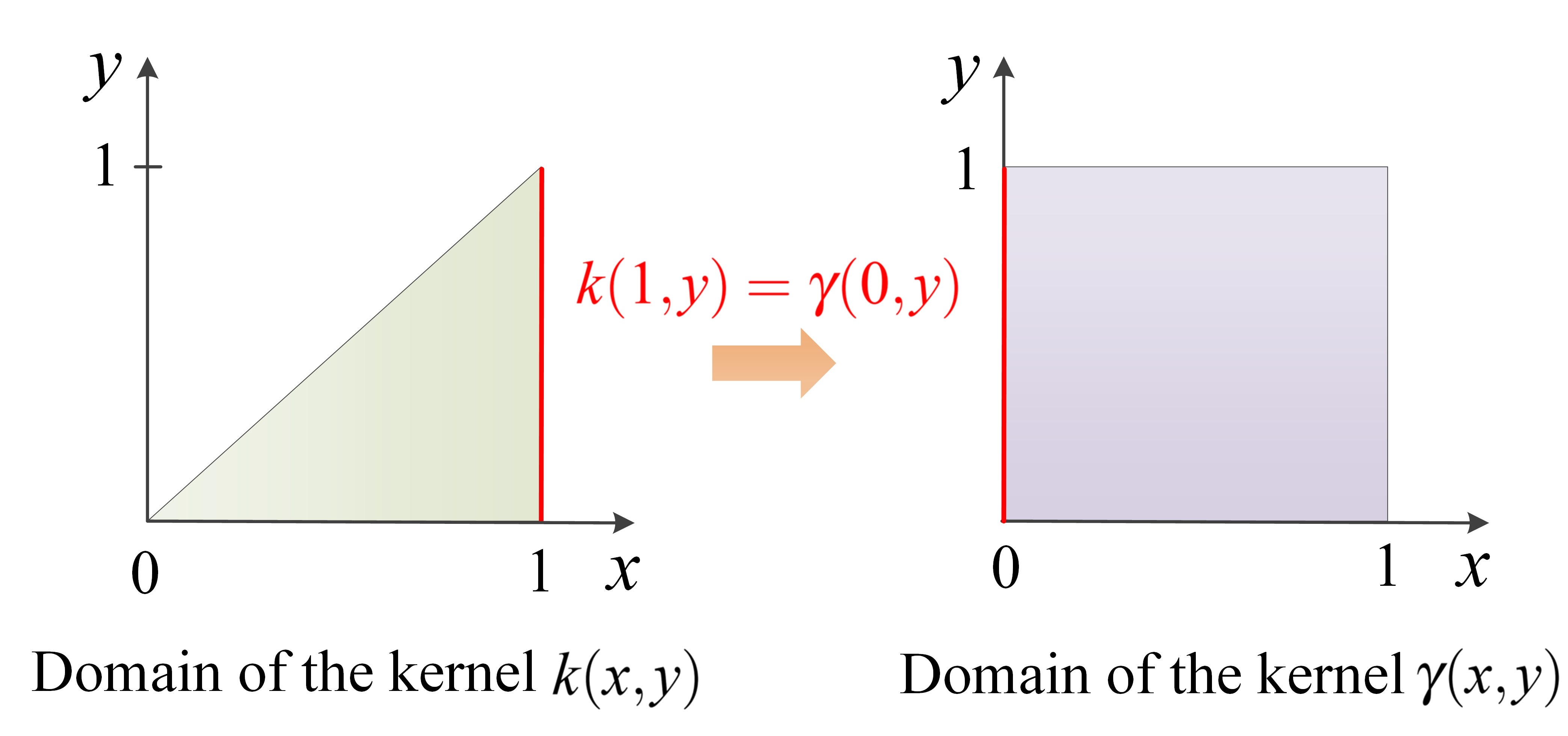
Figure 1: Triangular and rectangular domains of the gain kernel PDEs. Left: Goursat (backsteppign) kernel. Right: reaction-diffusion (predictor) kernel. Connection: Goursat/backstepping kernel serves as initial condition to reaction-diffusion/predictor kernel.

In the subsequent development, we treat (16)–(23) as a cascade of two nonlinear operators:

• the “Goursat kernel map” $\lambda\mapsto k$, whose output $k$ we shall refer to as the backstepping kernel,

• the “reaction-diffusion kernel map” $k\mapsto\gamma$, whose output $\gamma$ we refer to as the predictor kernel.

The domains of these two kernels (triangular for Goursat, and rectangular for reaction-diffusion), and their cascade connection, are depicted in Figure 1.

For the implementation of the controller in (24), whose gains are $\gamma(1,y)$ and $q(1-y)=-\gamma_{y}(1-y,1)$, the operator of interest is the composition operator $\lambda\mapsto\gamma$.

III Accuracy of Approximation of Backstepping Kernel Operator with DeepONet

III-A Boundedness of the gain kernel functions

In this section we establish smoothness and furnish bounds on the kernels of the backstepping transformations.

Lemma 1.

[bound on Goursat kernel] For every $\lambda\in C^{1}([0,1])$, the gain kernel $k(x,y)$ satisfying the PDE system (16)–(18) has a unique $C^{2}(\Omega_{1})$ solution with the following property

$$|k(x,y)|\leq\bar{\lambda}{\rm e}^{2\bar{\lambda}x},\quad\forall(x,y)\in\Omega_{1},$$ (25)

where $\bar{\lambda}=\sup_{x\in[0,1]}|\lambda(x)|$.

Proof.

In [37, 24]. $\blacksquare$

Next, we turn our attention to the backstepping kernel functions $\gamma$ and $q$. We introduce a space ${\Upsilon}\subset C^{1}((0,1]\times[0,1])$ of functions $\gamma(x,y)$ satisfying $\gamma[x]\in C^{2}([0,1])$ for all $x\in(0,1]$, namely, functions of two variables which are differentiable at least once in the first variable and at least twice in the second variable, for all positive values of the first variable.

The next lemma is useful for providing the bounds for the gain kernels $\gamma(x,y)$ and $q(x)=-\gamma_{y}(x,1)$, based on (27).

Lemma 2.

[bound on reaction-diffusion kernel, with Goursat kernel as initial condition] For every $\lambda,\ k(1,\cdot)\in C^{1}([0,1])$, the gain kernel $\gamma(x,y)$ satisfying the PDE system (19)–(22) has a unique solution in the function space $\Upsilon$ with the following property, for all $(x,y)\in\Omega_{2}$:

$$|\gamma(x,y)|^{2}\leq {\rm e}^{2D\bar{\lambda}x}\int_{0}^{1}(k(1,y)^{2}+k_{y}(1,y)^{2})\mathrm{d}y,$$ (26)

$$|\gamma_{y}(x,1)|^{2}\leq (1+2D\bar{\lambda})\bar{\lambda}{\rm e}^{2D\bar{\lambda}x}\int_{0}^{1}k(1,y)^{2}\mathrm{d}y$$

$$+\left(1+\bar{\lambda}+\frac{1}{D}\right){\rm e}^{2D\bar{\lambda}x}\int_{0}^{1}k_{y}(1,y)^{2}\mathrm{d}y.$$

$$+2D{\rm e}^{2D\bar{\lambda}x}\int_{0}^{1}k_{yy}(1,y)^{2}\mathrm{d}y.$$ (27)

Proof.

In Appendix A. $\blacksquare$

III-B Approximation of the neural operators

The controller (24) employs the gain functions $\gamma(1,y)$ and $-\gamma_{y}(1-y,1)$, which are both obtained from the predictor kernel $\gamma$, which is governed by PDE (19)–(22). This PDE has $k(1,y)$ as its initial condition, while, in turn, the backstepping kernel $k$’s PDE (16)–(18) is driven by function $\lambda$.

In summary, to implement controller (24), one needs to generate the output function $\gamma$ of the operator composition $\lambda\mapsto k\mapsto\gamma$, i.e., of the backstepping-predictor kernel cascade, for a given input function $\lambda$.

Hence, our controller implementation calls for a neural approximation of the composition mapping $\lambda\mapsto\gamma$. In more precise terms, since the PDE (19)–(22) depends not only on the initial condition $k(1,y)$ but also on the reactivity $\lambda(y)$, we need a neural approximation of two operators, $\lambda\mapsto k$ and $(\lambda,k(1,\cdot))\mapsto\gamma$, as shown in Figure 2.

Denote the sets of functions

$$\underline{K}=\{k\in C^{2}(\Omega_{1})|k(x,0)=0,\quad\forall x\in[0,1]\},$$ (28)

$$\underline{\Gamma}=\{\gamma\in\Upsilon|\gamma(x,0)=\gamma(x,1)=0,\quad\forall x\in[0,1]\},$$ (29)

and define the operators ${\mathcal{K}_{1}}:C^{1}[0,1]\to\underline{K}$ and ${\mathcal{K}_{2}}:C^{1}[0,1]\times C^{1}[0,1]\to\underline{\Gamma}$, where

$${\mathcal{K}_{1}}(\lambda)(x,y) := k(x,y),$$ (30)

$${\mathcal{K}_{2}}(\lambda,k(1,\cdot))(x,y) := \gamma(x,y),$$ (31)

respectively. This allows to introduce the operators ${\mathcal{M}}_{1}:C^{1}[0,1]\to\underline{K}\times C^{1}[0,1]\times\Upsilon$ defined by

$${\mathcal{M}}_{1}(\lambda)(x,y) :=(k(x,y),K_{1}(x),K_{2}(x,y))\,,$$ (32)

where

$$K_{1}(x)=2\frac{\mathrm{d}}{\mathrm{d}x}(k(x,x))+\lambda(x),$$ (33)

$$K_{2}(x,y)=k_{xx}(x,y)-k_{yy}(x,y)-\lambda(y)k(x,y),$$ (34)

and $\mathcal{M}_{2}:C^{1}[0,1]\times C^{1}[0,1]\to\underline{\Gamma}\times\Upsilon$ defined by

$${\mathcal{M}}_{2}(\lambda,k(1,\cdot))(x,y):=(\gamma(x,y),\Gamma(x,y)),$$ (35)

where

$$\Gamma(x,y)=\gamma_{x}(x,y)-D\gamma_{yy}(x,y)-D\lambda(y)\gamma(x,y).$$ (36)

For the operators $\mathcal{M}_{1}$ and $\mathcal{M}_{2}$, we establish the following approximation theorem using [8, Thm. 2.1].

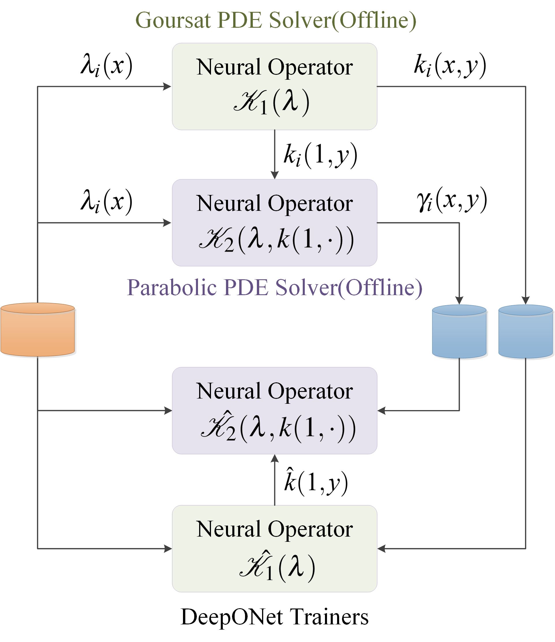
Figure 2: The process of learning the PDE backstepping design in DeepONet involves two operators: (1) for the first operator, $\lambda\mapsto k$, we compute multiple solutions of a kernel PDE (16)–(18) in the Goursat form by substituting different functions $\lambda_{i}$. (2) For the second operator described by the mapping $(\lambda,\ k(1,\cdot))\mapsto\gamma$, we solve the kernel PDE(19)–(22), which form likes a parabolic PDE, using the discretized form of the three-point difference method. This process is repeated multiple times with various functions $\lambda_{i}$ and their corresponding $k(1,y)$ values. After this step, the neural operators $\hat{\mathcal{K}}_{i},\ i=1,2$ are trained.

Theorem 1.

[DeepONet approximation of kernels] Consider the neural operators defined in (32) and (35), along with (33), (34), (36), (16)–(22). For all $B_{\lambda},\ B_{\lambda^{\prime}},\ B_{\lambda^{\prime\prime}}>0$ and $\epsilon>0$, there exist neural operators $\hat{{\mathcal{M}}}_{1}:C^{1}[0,1]\to\underline{K}\times C^{1}[0,1]\times\Upsilon$ and $\hat{\mathcal{M}}_{2}:C^{1}[0,1]\times C^{1}[0,1]\to\underline{\Gamma}\times\Upsilon$ such that,

$$|{\mathcal{M}}_{1}(\lambda)(x,y)-\hat{\mathcal{M}}_{1}(\lambda)(x,y)|$$

$$+|{\mathcal{M}}_{2}(\lambda,k(1,\cdot))(x,y)-\hat{\mathcal{M}}_{2}(\lambda,k(1,\cdot))(x,y)|<\epsilon,$$ (37)

holds for all Lipschitz $\lambda,\ k$ with the properties that $\rVert\lambda\rVert_{\infty}\leq B_{\lambda}$, $\rVert\lambda^{\prime}\rVert_{\infty}\leq B_{\lambda^{\prime}}$, $\rVert\lambda^{\prime\prime}\rVert_{\infty}\leq B_{\lambda^{\prime\prime}}$, namely, there exists neural operators $\hat{\mathcal{K}}_{i},\ i=1,\ 2$ such that $\hat{\mathcal{K}}_{1}(\lambda)(x,0)\equiv 0,\hat{\mathcal{K}}_{2}(\lambda,k(1,\cdot))(x,0)=\hat{\mathcal{K}}_{2}(\lambda,k(1,\cdot))(x,1)\equiv 0$, and

$$|\tilde{k}(x,y)|+|2\frac{\mathrm{d}}{\mathrm{d}x}(\tilde{k}(x,x)|+|\tilde{k}_{xx}(x,y)-\tilde{k}_{yy}(x,y)-\lambda(y)\tilde{k}(x,y)|$$

$$+|\tilde{\gamma}(x,y)|+|\tilde{\gamma}_{x}(x,y)|+|\tilde{\gamma}_{x}(x,y)-D\tilde{\gamma}_{yy}(x,y)-D\lambda(y)\tilde{\gamma}(x,y)|$$

$$|\tilde{k}_{yyy}(x,y)|+|\tilde{\gamma}_{y}(x-y,1)|+|\tilde{\gamma}_{xy}(x-y,1)|<\epsilon,$$ (38)

where

$$\tilde{k}(x,y)= k(x,y)-\hat{k}(x,y)$$

$$= {\mathcal{K}}_{1}(\lambda)(x,y)-\hat{\mathcal{K}}_{1}(\lambda)(x,y),$$ (39)

$$\tilde{\gamma}(x,y)= \gamma(x,y)-\hat{\gamma}(x,y)$$

$$= {\mathcal{K}}_{2}(\lambda,k(1,\cdot))(x,y)-\hat{\mathcal{K}}_{2}(\lambda,k(1,\cdot))(x,y).$$ (40)

Proof.

The continuity of the operators $\mathcal{M}_{1}$ and $\mathcal{M}_{2}$ follows from Lemmas 1 and 2, respectively. The result is obtained by invoking [8, Thm. 2.1]. $\blacksquare$

Instead of approximating the multi-input map $(\mathcal{M}_{1},\mathcal{M}_{2})$ in Theorem 1, we can obtain the remaining results of the paper also by considering the composition operator $\mathcal{M}=(\mathcal{M}_{1},\mathcal{M}_{2}(\mathcal{M}_{1})):\lambda\mapsto(k,K_{1},K_{2},\gamma,\Gamma)$, whose sole input function is $\lambda$. This appears more elegant but, in actual learning of the neural version of the operator, $\hat{\mathcal{M}}$, the training loss is bigger than for the neural operator $(\hat{\mathcal{M}}_{1},\hat{\mathcal{M}}_{2})$, especially for smaller datasets, so we stick with the approach in Theorem 1.

In Section IV, Theorem 1 enables us to prove exponential stabilization of (4)–(8) with the control law (24) when the gain kernels are approximated via DeepOnet using a collection of input-output data generated with the spatially varying reactivity $\lambda(x)$. For the control loop depicted in Figure 3, we prove that the gain learned offline as a DeepOnet enforces closed-loop stability with a quantifiable exponential decay rate.

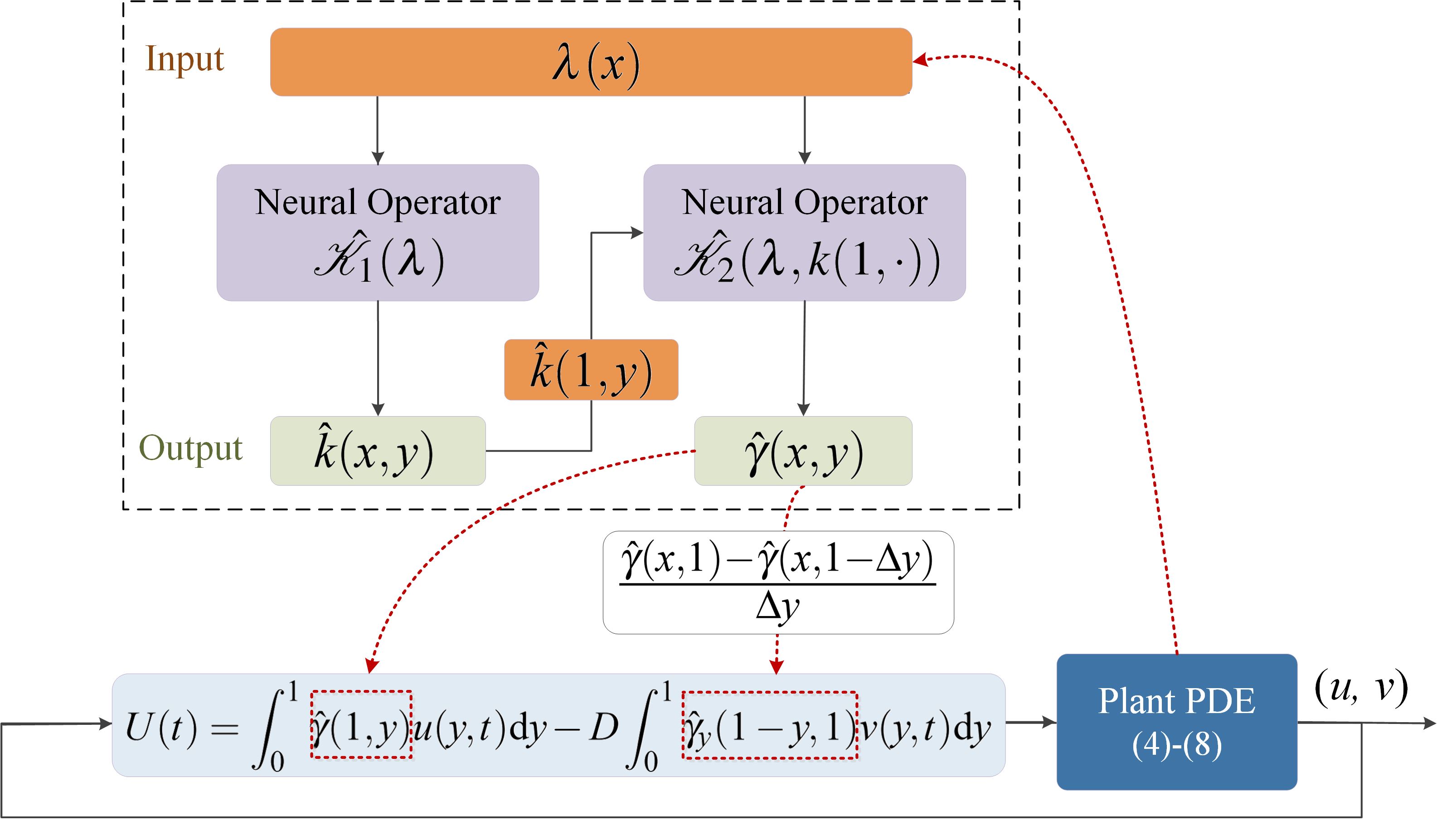
Figure 3: In the PDE backstepping control, the gain kernels are defined as $\gamma(x,y)$ and $\gamma_{y}(1-y,1)$. The first gain kernel is generated by the DeepONet $\hat{\mathcal{K}}_{i},\ i=1,2$, is implemented by incorporating the learned neural operators into the control system, while the second gain kernel is obtained by numerically differentiating the first gain kernel directly.

IV Stabilization under DeepONet Gain Feedback

The backstepping transformations (14), (15) fed by the approximate gain kernel $\hat{k}(x,y)$ are defined as

$$\hat{w}(x,t)= u(x,t)-\int_{0}^{x}\hat{k}(x,y)u(y,t)\mathrm{d}y,$$ (41)

$$\hat{z}(x,t)= v(x,t)-\int_{0}^{1}\hat{\gamma}(x,y)u(y,t)\mathrm{d}y$$

$$-D\int_{0}^{x}\hat{q}(x-y)v(y,t)\mathrm{d}y,$$ (42)

where $\hat{k}=\hat{\mathcal{K}}_{1}(\lambda)$, $\hat{\gamma}=\hat{\mathcal{K}}_{2}(\lambda,k(1,\cdot))$ and $\hat{q}(x)=-\hat{\gamma}_{y}(x,1)$ together with the approximate control law

$$U(t)=\int_{0}^{1}\hat{\gamma}(1,y)u(y,t)\mathrm{d}y-D\int_{0}^{1}\hat{\gamma}_{y}(1-y,1)v(y,t)\mathrm{d}y.$$ (43)

By differentiation, equations (41), (42) and (16)–(23) generate the perturbed target system given below

$$\hat{w}_{t}(x,t) =\hat{w}_{xx}(x,t)+\delta_{1}(x)u(x,t)+\int_{0}^{x}\delta_{2}(x,y)u(y,t)\mathrm{d}y,$$ (44)

$$\hat{w}(0,t) =0,$$ (45)

$$\hat{w}(1,t) =\hat{z}(0,t),$$ (46)

$$D\hat{z}_{t}(x,t) =\hat{z}_{x}(x,t)+\int_{0}^{1}\delta_{3}(x,y)u(y,t)\mathrm{d}y,$$ (47)

$$\hat{z}(1,t) =0,$$ (48)

where $\delta_{i},\ i=1,2,3$ are defined as

$$\delta_{1}(x)= 2\frac{\mathrm{d}}{\mathrm{d}x}\hat{k}(x,x)+\lambda(x)$$

$$= -2\frac{\mathrm{d}}{\mathrm{d}x}\tilde{k}(x,x),$$ (49)

$$\delta_{2}(x,y)= \hat{k}_{xx}(x,y)-\hat{k}_{yy}(x,y)-\lambda(y)\hat{k}(x,y)$$

$$= -\tilde{k}_{xx}(x,y)+\tilde{k}_{yy}(x,y)+\lambda(y)\tilde{k}(x,y),$$ (50)

$$\delta_{3}(x,y)= \hat{\gamma}_{x}(x,y)-D\hat{\gamma}_{yy}(x,y)-D\lambda(y)\hat{\gamma}(x,y)$$

$$= -\tilde{\gamma}_{x}(x,y)+D\tilde{\gamma}_{yy}(x,y)+D\lambda(y)\tilde{\gamma}(x,y).$$ (51)

Note that from (1), the following inequalities hold

$$\rVert\delta_{i}\rVert_{\infty}\leq\epsilon,\quad i=1,2,3,$$ (52)

$$\rVert\delta_{3x}\rVert_{\infty}\leq\epsilon.$$ (53)

Our first result for the closed-loop system is its exponential stability in the backstepping-transformed variables under the DeepONet-approximated kernels.

Proposition 1.

[Lyapunov analysis for DeepONet-perturbed target system] Consider the target system (44)–(48). For each $D>0$, there exists $\varepsilon^{*}>0$ such that for all $\varepsilon\in(0,\varepsilon^{*})$ there exist $c_{1},\ c_{2}>0$ such that the following holds,

$$\Psi_{1}(t)\leq\Psi_{1}(0)c_{2}{\rm e}^{-c_{1}t},\quad\forall\geq 0,$$ (54)

where

$$\Psi_{1}(t)=\rVert\hat{w}(t)\rVert^{2}+\rVert\hat{z}(t)\rVert^{2}+\rVert\hat{z}_{x}(t)\rVert^{2}.$$ (55)

The proof of Proposition 1 is given in Appendix B.

To translate the stability of the target system into that of the original closed-loop system, we consider transformations (41) and (42), along with their inverse transformations,

$$u(x,t)= \hat{w}(x,t)+\int_{0}^{x}\hat{l}(x,y)\hat{w}(y,t)\mathrm{d}y,$$ (56)

$$v(x,t)= \hat{z}(x,t)+\int_{0}^{1}\hat{\eta}(x,y)\hat{w}(y,t)\mathrm{d}y$$

$$+D\int_{0}^{x}\hat{p}(x-y)\hat{z}(y,t)\mathrm{d}y,$$ (57)

and provide the following proposition.

Proposition 2.

[norm equivalence with DeeepONet kernels] The following estimates hold between the plant (4)–(8) and the target system (44)–(48),

$$S_{1}\Psi_{1}(t)\leq\Phi(t)\leq S_{2}\Psi_{1}(t)$$ (58)

where

$$\Phi(t)=\rVert u(t)\rVert^{2}+\rVert v(t)\rVert^{2}+\rVert v_{x}(t)\rVert^{2},$$ (59)

and the positive constants

$$S_{1}= 9+2\int_{0}^{1}\int_{0}^{x}\hat{k}(x,y)^{2}\mathrm{d}x\mathrm{d}y+3\int_{0}^{1}\int_{0}^{1}\hat{\gamma}(x,y)^{2}\mathrm{d}x\mathrm{d}y$$

$$+4\int_{0}^{1}\int_{0}^{1}\hat{\gamma}_{x}(x,y)^{2}\mathrm{d}x\mathrm{d}y+3D^{2}\int_{0}^{1}\int_{0}^{x}\hat{q}(x-y)^{2}\mathrm{d}x\mathrm{d}y$$

$$+4D^{2}\hat{q}(0)^{2}+4D^{2}\int_{0}^{1}\int_{0}^{x}\hat{q}^{\prime}(x-y)^{2}\mathrm{d}x\mathrm{d}y,$$ (60)

$$S_{2}= 9+2\int_{0}^{1}\int_{0}^{x}\hat{l}(x,y)^{2}\mathrm{d}x\mathrm{d}y+3\int_{0}^{1}\int_{0}^{1}\hat{\eta}(x,y)^{2}\mathrm{d}x\mathrm{d}y$$

$$+4\int_{0}^{1}\int_{0}^{1}\hat{\eta}_{x}(x,y)^{2}\mathrm{d}x\mathrm{d}y+3D^{2}\int_{0}^{1}\int_{0}^{x}\hat{p}(x-y)^{2}\mathrm{d}x\mathrm{d}y$$

$$+4D^{2}\hat{p}(0)^{2}+4D^{2}\int_{0}^{1}\int_{0}^{x}\hat{p}^{\prime}(x-y)^{2}\mathrm{d}x\mathrm{d}y$$ (61)

are bounded.

Proof.

In Appendix C. Similar to proof of [41, Prop. 1]. $\blacksquare$

Based on the norm-equivalence in Proposition 2, the main result in the next theorem immediately follows from Proposition 1.

Theorem 2.

[main result—stabilization with DeepONet] Consider the system (4)–(8) or, equivalently, system (1)–(3), with any $\lambda\in{C}^{1}([0,1])$ whose derivatives $\lambda^{\prime}$ and $\lambda^{\prime\prime}$ are Lipschitz and which satisfy $\rVert\lambda\rVert_{\infty}\leq B_{\lambda}$, $\rVert\lambda^{\prime}\rVert_{\infty}\leq B_{\lambda^{\prime}}$, $\rVert\lambda^{\prime\prime}\rVert_{\infty}\leq B_{\lambda^{\prime\prime}}$, and $B_{\lambda},\ B_{\lambda^{\prime}},\ B_{\lambda^{\prime\prime}}>0$. There exists a sufficiently small $\epsilon^{*}(B_{\lambda},\ B_{\lambda^{\prime}},\ B_{\lambda^{\prime\prime}})>0$, such that the feedback controller

$$U(t)=\int_{0}^{1}\hat{\gamma}(1,y)u(y,t)\mathrm{d}y-D\int_{0}^{1}\hat{\gamma}_{y}(1-y,1)v(y,t)\mathrm{d}y,$$ (62)

with two neural operators $\hat{\mathcal{M}}_{i},\ i=1,2$ of approximation accuracy $\epsilon\in(0,\epsilon^{*})$, in relation to the exact backstepping kernels $k(x,y)$ and $\gamma(x,y)$, respectively, ensure that the closed-loop system satisfies the following exponential stability bound,

$$\Phi(t)\leq\Phi(0)\frac{S_{2}}{S_{1}}c_{2}{\rm e}^{-c_{1}t}\,,\quad\forall t\geq 0\,.$$ (63)

V Simulation of the Stability results under the NO approximated gain kernels

Our simulation is for a reaction-diffusion PDE with a boundary input delay $D=2$ and a spatially varying reactivity coefficient $\lambda(x)=10.2+$ $2\cos(\Gamma\cos^{-1}(x))$ parameterized by $\Gamma=[5,10]$, which renders the PDE unstable for all $\Gamma$s in that range. The closed-loop system with the nominal, delay-uncompensated backstepping controller is unstable as shown in Figure 4 with the spatial step $\Delta x=0.005$ and the temporal step $\Delta t=0.0001$. Additionally, the plots of the reaction terms depicted in Figure 5 show that the intensity of the oscillations of $\lambda$ is an increasing function of $\Gamma$, leading to a lower rate of instability, as indicated on the right side of Figure 5.

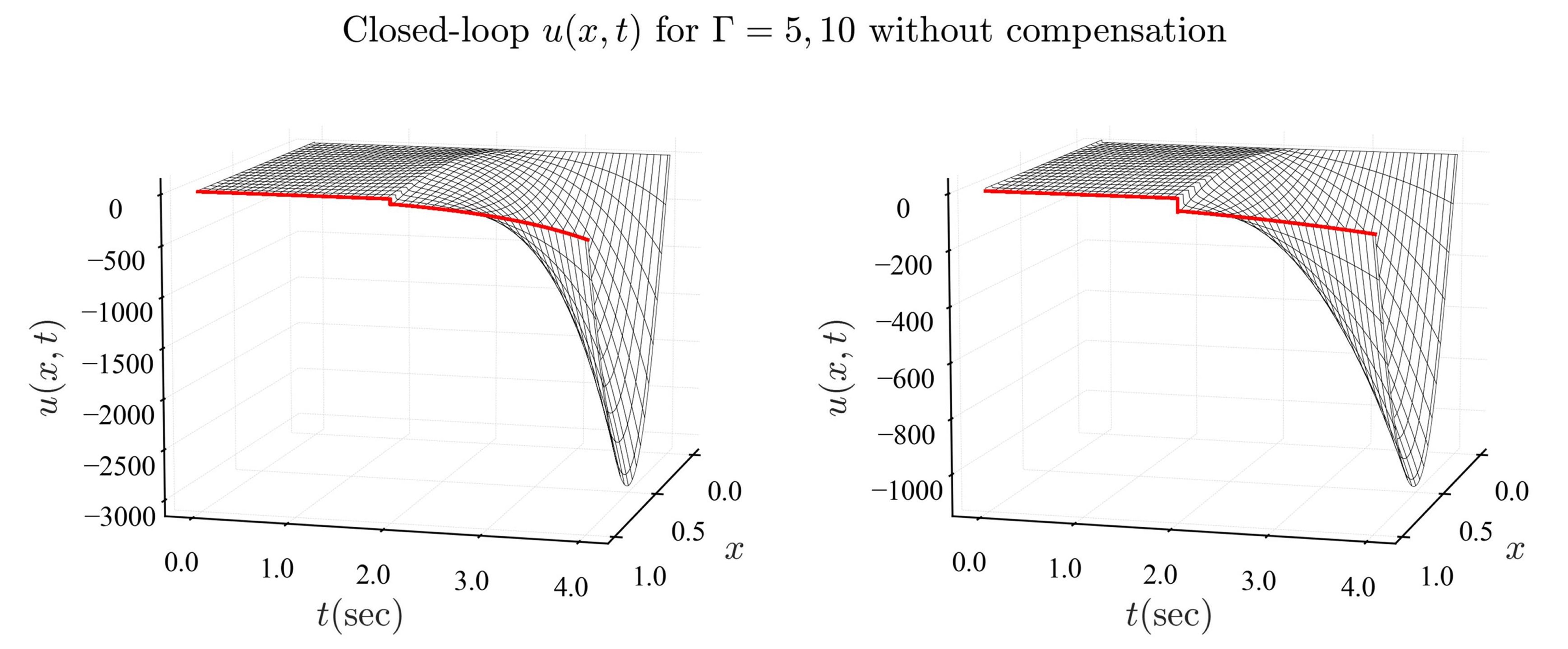
Figure 4: Instability of the closed-loop system with reaction coefficients defined as $\lambda(x)=10.2+2\cos(\Gamma\cos(x)^{-1})$, $\Gamma=5,\ 10$, respectively, under the control law of the delay-free plant [24] for a constant initial condition $u_{0}(x)=10$.

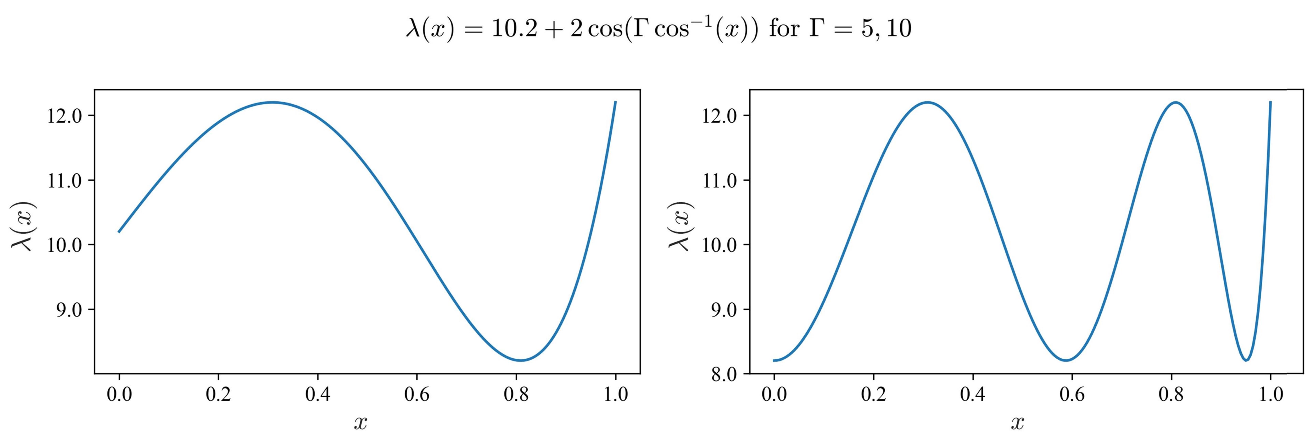
Figure 5: The reaction coefficients $\lambda(x)=10.2+2\cos(\gamma\cos(x)^{-1})$ with $\gamma=5,\ 10$, respectively.

As opposed to [24], we consider learning the two kernels $k(x,y)$ and $\gamma(x,y)$, which can be achieved in two steps by defining the mappings $\mathcal{K}_{1}:\lambda\mapsto k$ and $\mathcal{K}_{2}:(\lambda,\ k(1,\cdot))\mapsto\gamma$. The first learning step has been performed in [24] but, for the second step, a DeepONet with two inputs and one output is required. The training of our neural network on the approximate kernel $\gamma(x,y)$ is accomplished by passing the training of two datasets of different $\lambda(x)$ and $k(1,y)$ with a given range of the parameter $\Gamma$, namely, $\Gamma\in[5,10]$, uniformly distributed through the network.

Data Sets (train/test)	Training Time (sec)	Average Relative Error Training Data	Average Relative Error Testing Data	Average Calculation Time CPU (sec)	Average Calculation Time GPU (sec)
500 (450/50)	325.76	$1.02\times 10^{-2}$	$1.05\times 10^{-2}$	$1.09$	$6.75\times 10^{-3}$
1000 (900/100)	609.84	$7.72\times 10^{-4}$	$7.86\times 10^{-4}$	$1.74$	$3.87\times 10^{-3}$
2000 (1800/200)	1201.61	$2.16\times 10^{-4}$	$2.44\times 10^{-4}$	$2.34$	$2.03\times 10^{-3}$

Table I: The relationship between different sizes of datasets and the accuracy of NO approximated $k$ under the parameter size 76169285. The best values are highlighted in blue.

Data Sets (train/test)	Training Time (sec)	Average Relative Error Training Data	Average Relative Error Testing Data	Average Calculation Time CPU (sec)	Average Calculation Time GPU (sec)
500 (450/50)	323.52	$9.94\times 10^{-3}$	$1.09\times 10^{-2}$	$1.41$	$7.97\times 10^{-3}$
1000 (900/100)	628.61	$2.78\times 10^{-3}$	$2.80\times 10^{-3}$	$1.50$	$3.82\times 10^{-3}$
2000 (1800/200)	1235.74	$9.92\times 10^{-4}$	$1.01\times 10^{-3}$	$2.34$	$2.03\times 10^{-3}$

Table II: The relationship between different sizes of datasets and the accuracy of NO approximated $\gamma$ under the parameter size 76169685. The most accurate approximations are highlighted in blue.

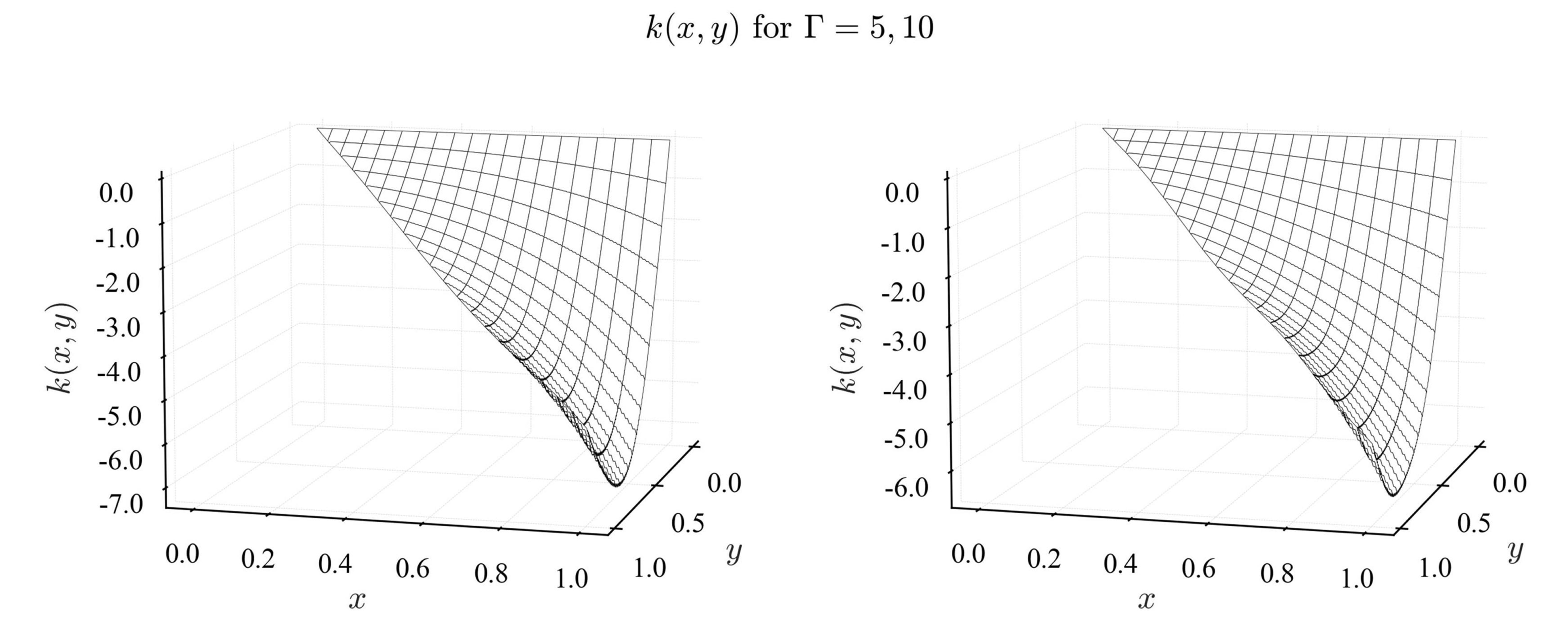
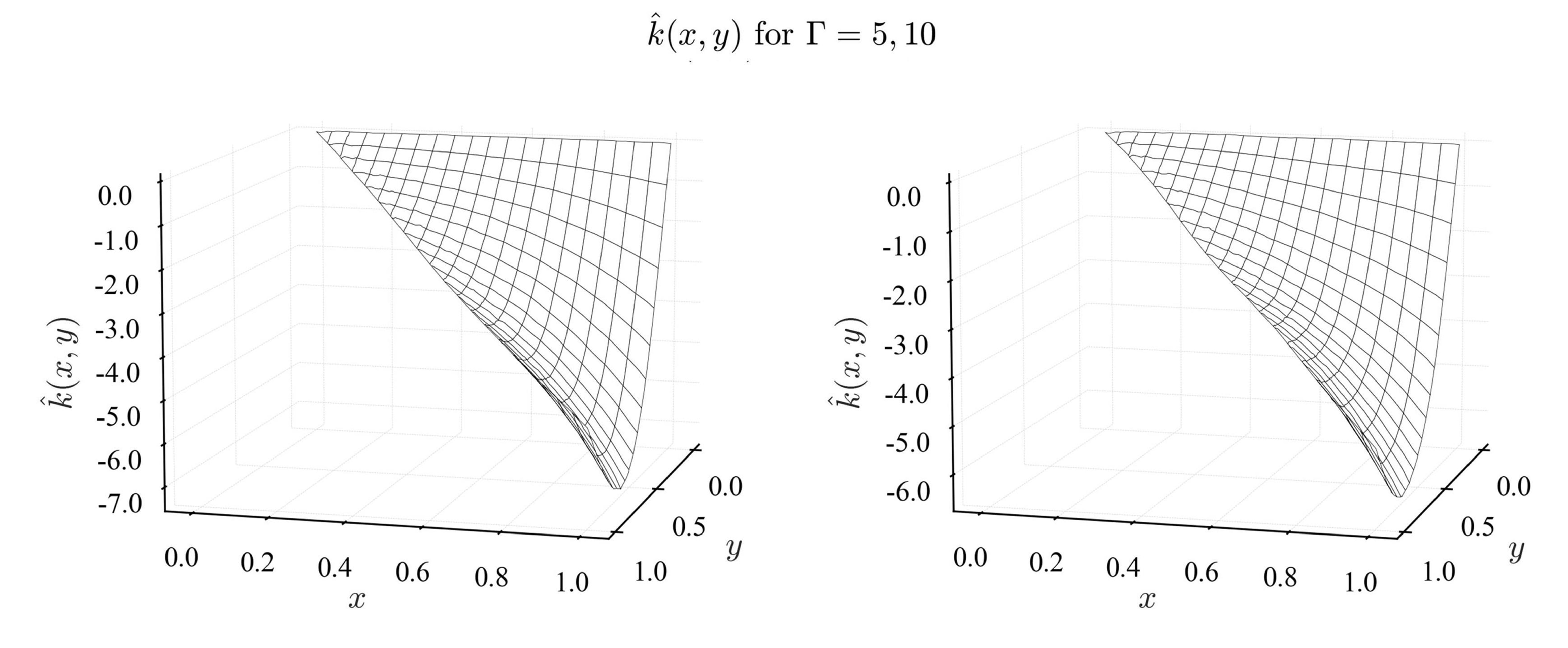
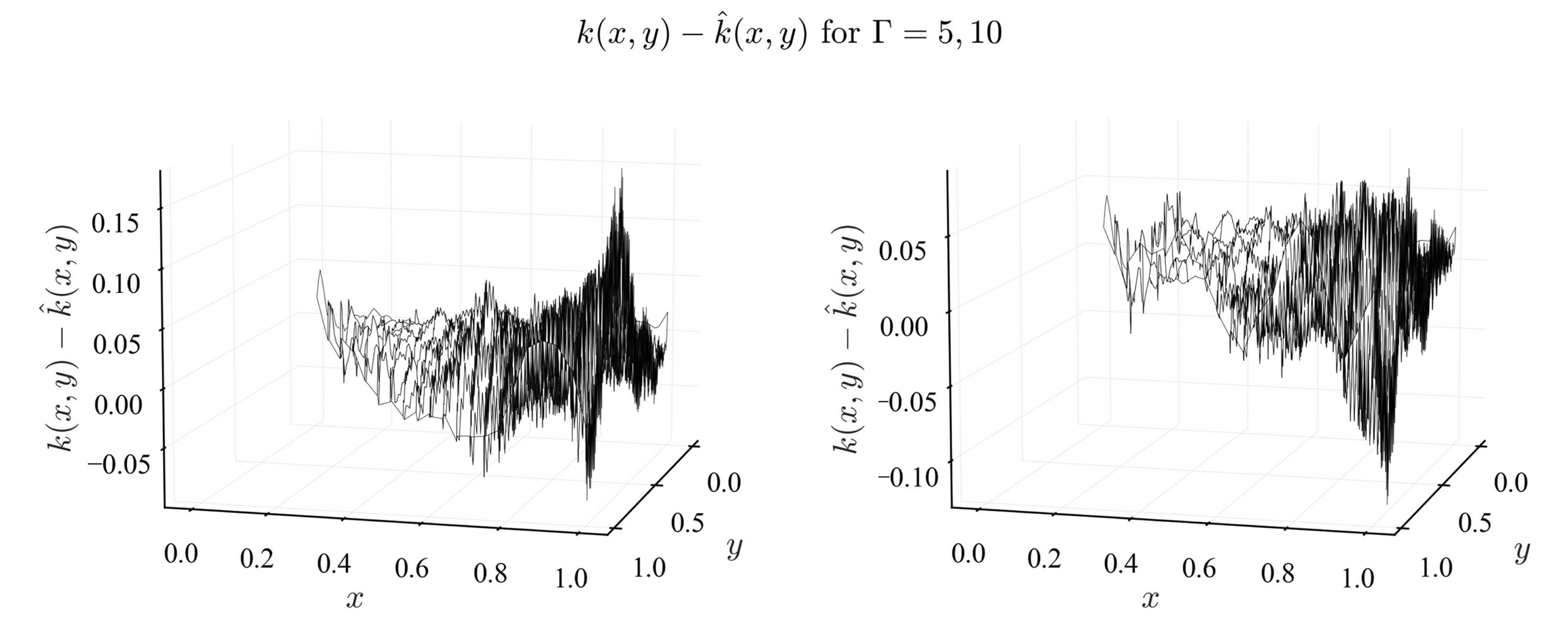
Figure 6: The kernels $k(x,y)$, $\hat{k}(x,y)$ and $k(x,y)-\hat{k}(x,y)$.

The DeepONet is efficiently used without an alteration of the grid, by iterating $\lambda(x)$ along the $y$-axis to generate a 2D input for $\mathcal{K}_{1}$ network. For similar reasons, $\lambda(x),\ k(1,y)$ along the $y$-axis and $x$-axis, respectively, are to create two 2D input for $\mathcal{K}_{2}$ network. Our approach leverages the 2D structure by employing a CNN for the DeepONet branch network. The relationship between various dataset sizes and the accuracy of the approximate values of $k$ and $\gamma$ is presented in Tables I and II, respectively. The stepsizes for $x$ and $y$ are both $0.005$. All experiments are run on an Nvidia Titan Xp (the CPU is Intel I7). Based on a dataset of size 2000, the model that achieves the utmost precision in classifying data points is obtained. Figures 6 and 7 illustrate the analytical and learned DeepONet kernels $k$ and $\gamma$, respectively, for the two $\Gamma$ values depicted in Figure 5. During the training process, see Figure 8, the relative $L^{2}$ errors for kernels $k(x,y)$ and $\gamma(x,y)$ are measured to be $2.16\times 10^{-4}$ and $9.92\times 10^{-4}$, while the testing error amounts to $2.44\times 10^{-4}$ and $1.01\times 10^{-3}$, respectively. By employing the learned neural operator, we achieve notable speedups, approximately on the order of $10^{3}$, compared to an efficient finite-difference implementation. To compute the approximate value of the controller signal given by (43), the value of $\hat{\gamma}_{y}(1-y,1)$ is needed, which can be obtained by using the estimate of $\hat{\gamma}_{y}(x,1)=\frac{\hat{\gamma}(x,1)-\hat{\gamma}(x,1-\Delta y)}{\Delta y}$. The simulations confirm closed-loop stability under a delay-compensated boundary control with kernel gains approximation as shown in Fig. 9.

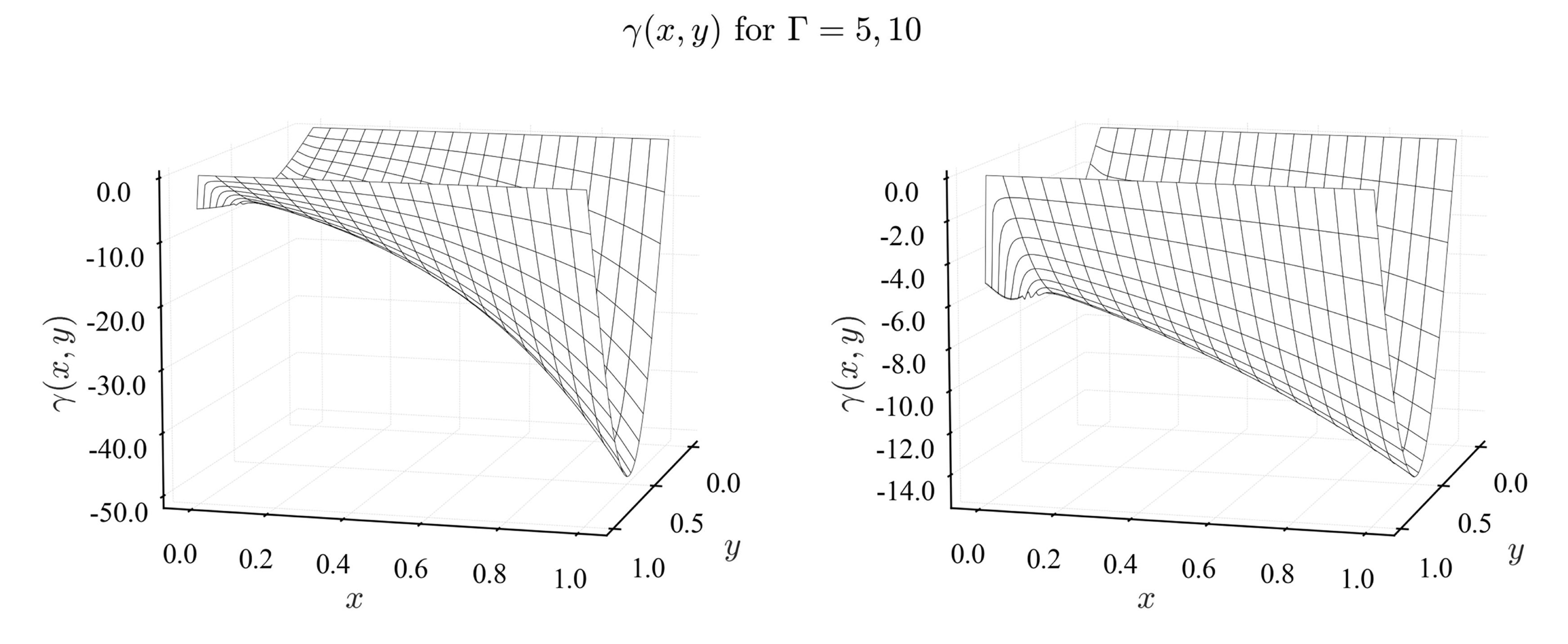
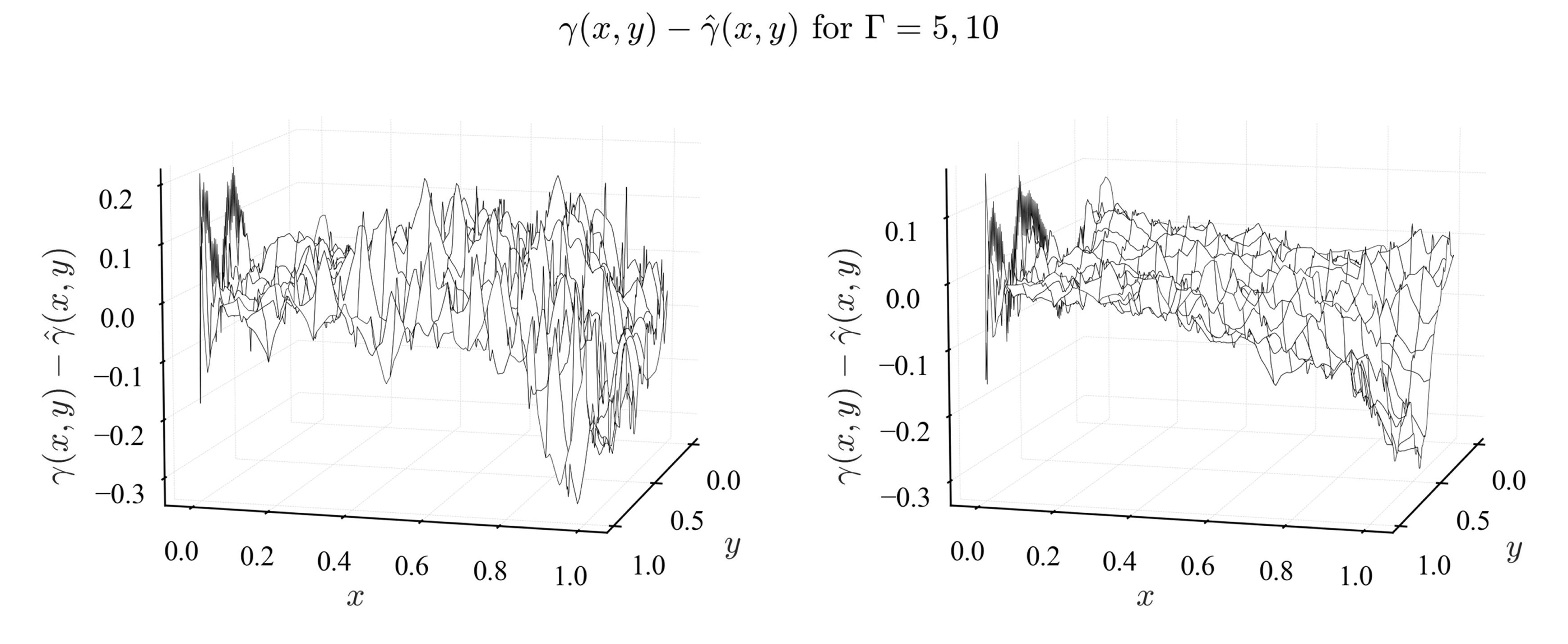
Figure 7: The kernels $\gamma(x,y)$, $\hat{\gamma}(x,y)$ and $\gamma(x,y)-\hat{\gamma}(x,y)$

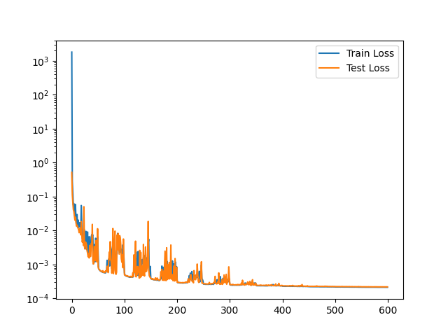
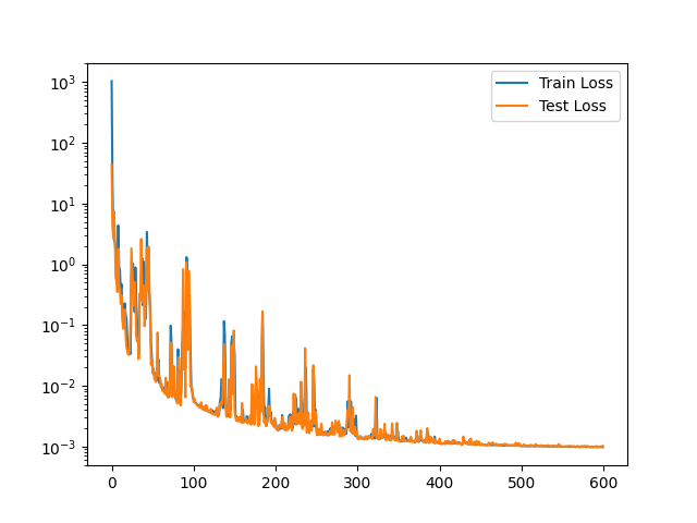
Figure 8: The train and test loss for $\lambda\mapsto k$ and $(\lambda,\ k(1,\cdot))\mapsto\gamma$.

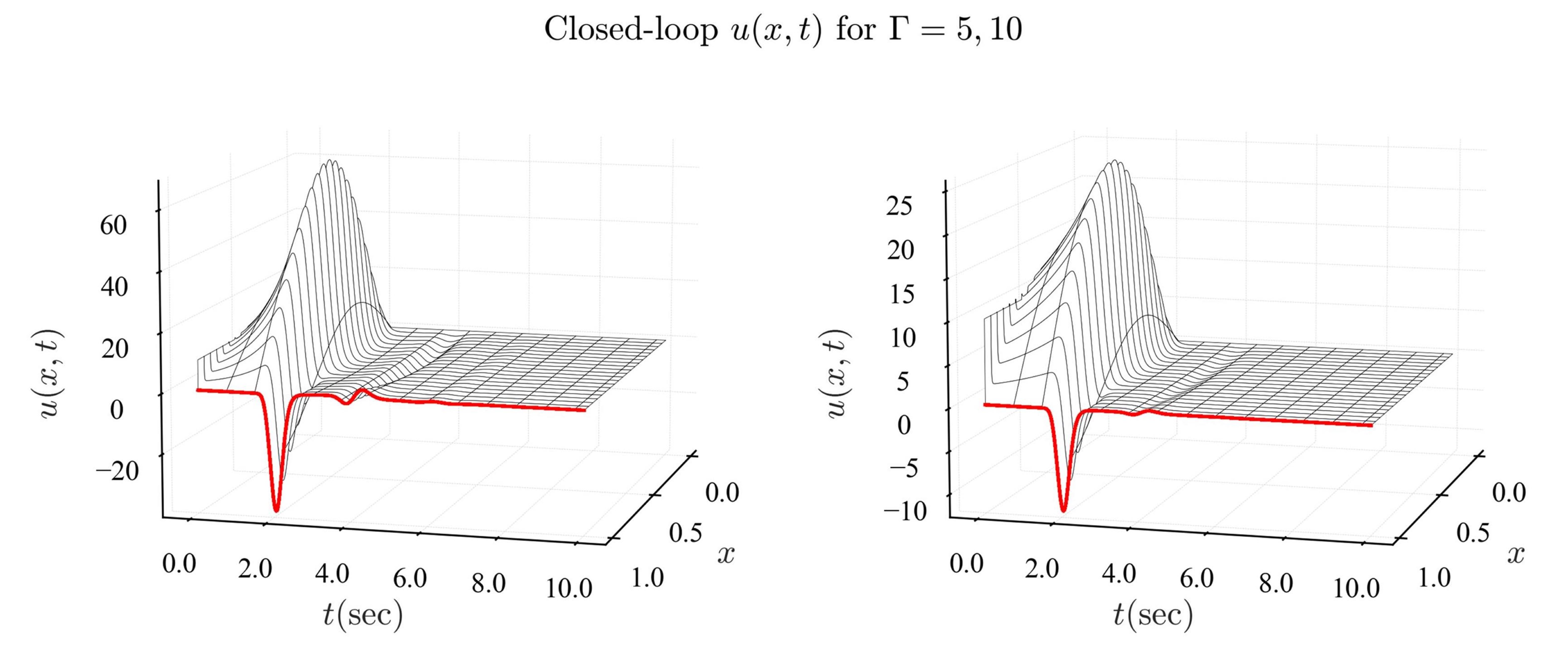
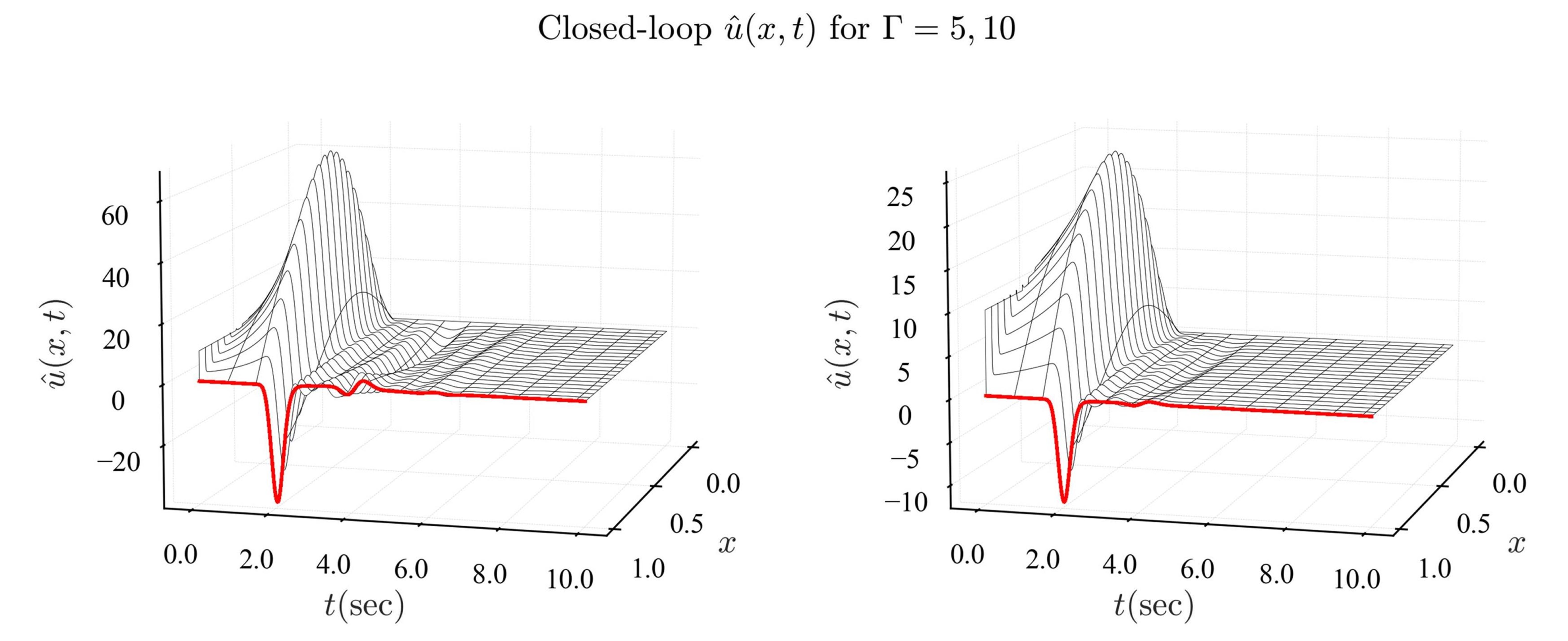
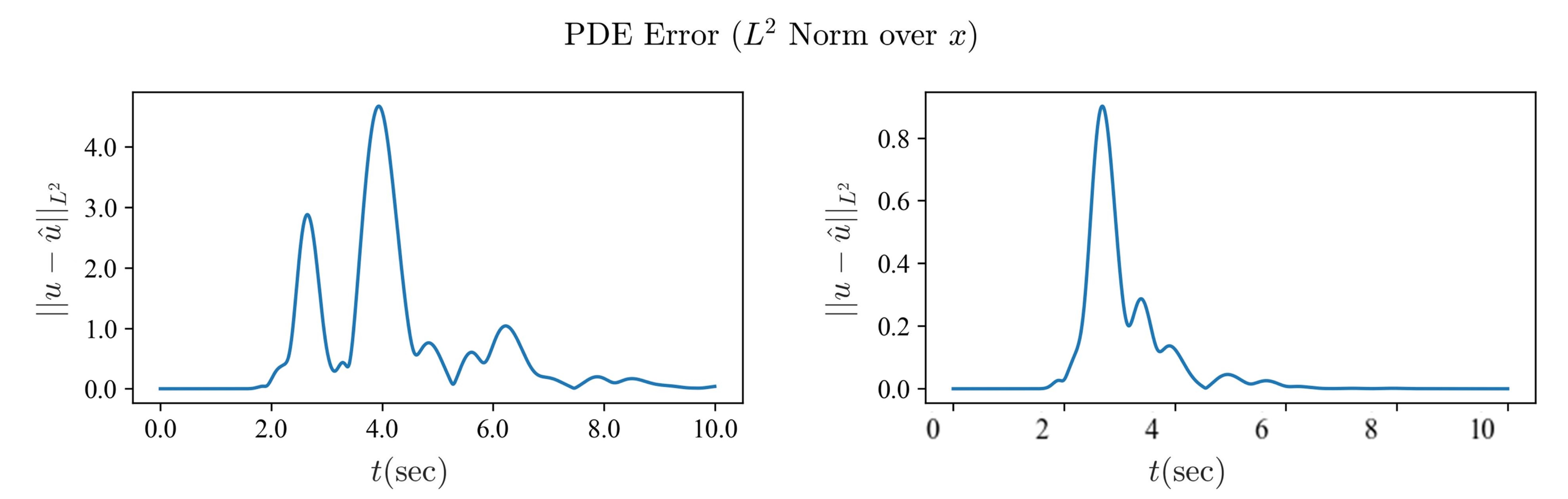
Figure 9: For the two respective values of $\lambda(x)$, the top row shows closed-loop solutions with kernels $k(x,y)$ and $\gamma(x,y)$, the middle row shows closed-loop solutions with the learned kernels $k(x,y)$ and $\gamma(x,y)$, and the bottom row shows the closed-loop PDE error between applying the original kernels $k(x,y),\ \gamma(x,y)$ and the learned kernels $k(x,y)$ and $\gamma(x,y)$.

VI Concluding Remarks

The papers [4], [24], and [35] introduced DeepONet approximations of PDE backstepping designs with single Goursat-form kernel PDEs for, respectively, hyperbolic, parabolic, and hyperbolic PDEs with input delays. By considering a backstepping design for a reaction-diffusion PDE with input delay in this paper, we demonstrate how to tackle problems where more than one kernel PDE, and belonging to different PDE classes, need to be approximated with a DeepONet, and their stabilizing capability proven using the universal approximation theorem for nonlinear operators [8].

The structure of the nonlinear operator being approximated is interesting and instructive. First, the reactivity function generates one backstepping kernel, which is a solution to a second-order parabolic Goursat PDE. Then, the solution of that Goursat PDE serves as an initial condition to another parabolic (reaction-diffusion) PDE, to generate a second (predictor) kernel. Each of the two PDEs, from distinct classes, gives rise to a separate nonlinear operator and, taken as a composition of operators, they generate a single nonlinear operator, from the reactivity function to the control gain functions. We approximate this overall nonlinear operator to generate the control input.

Thus, the extension of DeepONet-based PDE backstepping to compositions of kernel PDE-based nonlinear operators is the paper’s main technical contribution. The paper’s control contributions are the proofs of stabilization under the approximated kernels.

Appendix A Proof of Lemma 2

Let’s define the $L^{2}$ norm of function $f(x,t)\in L^{2}[0,1]$ as follows:

$$\rVert f(t)\rVert_{L^{2}}^{2}=\int_{0}^{1}|f(x,t)|^{2}\mathrm{d}x.$$ (64)

To prove Lemma 2, we start from the following lemma, which derives explicit bounds on the derivatives of $k(x,y)$, and then, after this lemma, turn our attention to $\gamma(x,y)$ from Lemma 2.

Lemma 3.

[bounds on Goursat kernel’s derivatives] For the function $k(x,y)$ satisfying the PDE system (16)–(18), the following holds:

$$|k_{y}(x,y)|^{2}\leq \frac{5\bar{\lambda}^{2}}{8}+{\bar{\lambda}^{4}}{\rm e}^{4\bar{\lambda}},$$ (65)

$$|k_{yy}(x,y)|^{2}\leq \frac{3(32\bar{\lambda}^{\prime 2}+31\bar{\lambda}^{4})}{256}$$

$$+\frac{3\bar{\lambda}^{2}(32\bar{\lambda}^{2}+26\bar{\lambda}^{\prime 2}+23\bar{\lambda}^{4})e^{4\bar{\lambda}}}{128},$$ (66)

$$|k_{yyy}(x,y)|^{2}\leq \frac{12\lambda^{\prime\prime 2}+73\bar{\lambda}^{\prime 2}\bar{\lambda}^{2}+218\bar{\lambda}^{4}+20\bar{\lambda}^{6}}{64}$$

$$+\frac{\bar{\lambda}^{2}{\rm e}^{4\bar{\lambda}}(36\bar{\lambda}^{\prime 2}(1+\bar{\lambda}^{2})+68\bar{\lambda}^{4}+19\bar{\lambda}^{\prime\prime 2})}{16}$$

$$+\frac{\bar{\lambda}^{4}e^{4\bar{\lambda}}(6\bar{\lambda}^{\prime 2}+119\bar{\lambda}^{4})}{128}.$$ (67)

Proof.

Let us start by defining

$$G(\xi,\eta)=k(x,y),$$ (68)

where $\xi=x-y,\ \eta=x-y$. Then,

$$k_{y}(x,y)=G_{\xi}(\xi,\eta)-G_{\eta}(\xi,\eta),$$ (69)

where

$$G_{\xi}(\xi,\eta)= -\frac{1}{4}\lambda\left(\frac{\xi}{2}\right)+\frac{1}{4}\int_{0}^{\eta}\lambda\left(\frac{\xi-s}{2}\right)G(\xi,s)\mathrm{d}s,$$ (70)

$$G_{\eta}(\xi,\eta)= \frac{1}{4}\lambda\left(\frac{\eta}{2}\right)-\frac{1}{4}\int_{0}^{\eta}\lambda\left(\frac{\eta-s}{2}\right)G(\eta,s)\mathrm{d}s$$

$$+\frac{1}{4}\int_{\eta}^{\xi}\lambda\left(\frac{\tau-\eta}{2}\right)G(\tau,\eta)\mathrm{d}\tau,$$ (71)

satisfy the following estimates

$$G_{\xi}(\xi,\eta)^{2}$$

$$= \bigg{(}-\frac{1}{4}\lambda\left(\frac{\xi}{2}\right)+\frac{1}{4}\int_{0}^{\eta}\lambda\left(\frac{\xi-s}{2}\right)G(\xi,s)\mathrm{d}s\bigg{)}^{2}$$

$$\leq \frac{\bar{\lambda}^{2}}{8}+\frac{\bar{\lambda}^{2}}{8}\int_{0}^{\eta}G(\xi,s)^{2}\mathrm{d}s$$

$$\leq \frac{\bar{\lambda}^{2}}{8}(1+\bar{\lambda}^{2}e^{4\bar{\lambda}}),$$ (72)

$$G_{\eta}(\xi,\eta)^{2}$$

$$= \bigg{(}\frac{1}{4}\lambda\left(\frac{\eta}{2}\right)-\frac{1}{4}\int_{0}^{\eta}\lambda\left(\frac{\eta-s}{2}\right)G(\eta,s)\mathrm{d}s$$

$$+\frac{1}{4}\int_{\eta}^{\xi}\lambda\left(\frac{\tau-\eta}{2}\right)G(\tau,\eta)\mathrm{d}\tau\bigg{)}^{2}$$

$$\leq \frac{3\bar{\lambda}^{2}}{16}+\frac{3\bar{\lambda}^{2}}{16}\int_{0}^{\eta}G(\eta,s)^{2}\mathrm{d}s+\frac{3\bar{\lambda}^{2}}{16}\int_{\xi}^{\eta}G(\tau,\eta)^{2}\mathrm{d}\tau$$

$$\leq \frac{3\bar{\lambda}^{2}}{16}(1+2\bar{\lambda}^{2}e^{4\bar{\lambda}}).$$ (73)

To arrive at (72), (73), we use the fact that $G(\xi,\eta)=k(x,y)$ and $|k(x,y)|\leq\bar{\lambda}{\rm e}^{2\bar{\lambda}x}$. Hence, based on (69), (72), and (73), one can get

$$k_{y}(x,y)^{2}\leq 2G_{\xi}(\xi,\eta)^{2}+2G_{\eta}(\xi,\eta)^{2}$$

$$\leq \frac{5\bar{\lambda}^{2}}{8}+{\bar{\lambda}^{4}}{\rm e}^{4\bar{\lambda}},$$ (74)

is bounded.

The next step is to find an upper bound of $k_{yy}(x,y)$. Knowing that

$$k_{yy}(x,y)=G_{\xi\xi}(\xi,\eta)-2G_{\xi\eta}(\xi,\eta)+G_{\eta\eta}(\xi,\eta),$$ (75)

where

$$G_{\eta\xi}(\xi,\eta)= -\frac{1}{4}\lambda\left(\frac{\xi-\eta}{2}\right)G(\xi,\eta),$$ (76)

$$G_{\xi\xi}(\xi,\eta)= -\frac{1}{8}\lambda^{\prime}\left(\frac{\xi}{2}\right)+\frac{1}{8}\int_{0}^{\eta}\lambda^{\prime}\left(\frac{\xi-s}{2}\right)G(\xi,s)\mathrm{d}s$$

$$+\frac{1}{4}\int_{0}^{\eta}\lambda\left(\frac{\xi-s}{2}\right)G_{\xi}(\xi,s)\mathrm{d}s,$$ (77)

$$G_{\eta\eta}(\xi,\eta)= \frac{1}{8}\lambda^{\prime}\left(\frac{\eta}{2}\right)-\frac{1}{8}\int_{0}^{\eta}\lambda^{\prime}\left(\frac{\eta-s}{2}\right)G(\eta,s)\mathrm{d}s$$

$$-\frac{1}{4}\int_{0}^{\eta}\lambda\left(\frac{\eta-s}{2}\right)G_{\eta}(\eta,s)\mathrm{d}s$$

$$-\frac{1}{8}\int_{\eta}^{\xi}\lambda^{\prime}\left(\frac{\tau-\eta}{2}\right)G(\tau,\eta)\mathrm{d}\tau$$

$$+\frac{1}{4}\int_{\eta}^{\xi}\lambda\left(\frac{\tau-\eta}{2}\right)G_{\eta}(\tau,\eta)\mathrm{d}\tau,$$ (78)

the following estimates

$$G_{\eta\xi}(\xi,\eta)^{2}\leq \frac{\bar{\lambda}^{4}{\rm e}^{4\bar{\lambda}}}{16},$$ (79)

$$G_{\xi\xi}(\xi,\eta)^{2}\leq \frac{3(2\bar{\lambda}^{\prime 2}+\bar{\lambda}^{4})}{128}+\frac{3\bar{\lambda}^{2}e^{4\bar{\lambda}}(2\bar{\lambda}^{\prime 2}+\bar{\lambda}^{4})}{128},$$ (80)

$$G_{\eta\eta}(\xi,\eta)^{2}\leq \frac{5(4\bar{\lambda}^{\prime 2}+5\bar{\lambda}^{4})}{256}+\frac{5\bar{\lambda}^{2}e^{4\bar{\lambda}}(\bar{\lambda}^{\prime 2}+\bar{\lambda}^{4})}{32},$$ (81)

can be deduced. Thus, from (75) and (79)–(81), one gets that

$$|k_{yy}(x,y)|^{2}\leq 12G_{\eta\xi}(\xi,\eta)^{2}+3G_{\xi\xi}(\xi,\eta)^{2}+3G_{\eta\eta}(\xi,\eta)^{2}$$ (82)

is bounded.

The last step is to prove the boundedness of $k_{yy}(1,y)$ and $k_{yyy}(1,y)$. From (75), we derive the following relation

$$k_{yyy}(x,y)= G_{\xi\xi\xi}(\xi,\eta)-3G_{\xi\xi\eta}(\xi,\eta)+3G_{\xi\eta\eta}(\xi,\eta)$$

$$-G_{\eta\eta\eta}(\xi,\eta),$$ (83)

where

$$G_{\eta\eta\xi}(\xi,\eta)= -\frac{1}{8}\lambda^{\prime}\left(\frac{\xi-\eta}{2}\right)G(\xi,\eta)$$

$$+\frac{1}{4}\lambda\left(\frac{\xi-\eta}{2}\right)G_{\eta}(\xi,\eta),$$ (84)

$$G_{\eta\xi\xi}(\xi,\eta)= \frac{1}{8}\lambda^{\prime}\left(\frac{\xi-\eta}{2}\right)G(\xi,\eta)$$

$$+\frac{1}{4}\lambda\left(\frac{\xi-\eta}{2}\right)G_{\xi}(\xi,\eta),$$ (85)

$$G_{\xi\xi\xi}(\xi,\eta)= -\frac{1}{16}\lambda^{\prime\prime}\left(\frac{\xi}{2}\right)+\frac{1}{4}\int_{0}^{\eta}\lambda\left(\frac{\xi-s}{2}\right)G_{\xi\xi}(\xi,s)\mathrm{d}s$$

$$+\frac{1}{4}\int_{0}^{\eta}\lambda^{\prime}\left(\frac{\xi-s}{2}\right)G_{\xi}(\xi,s)\mathrm{d}s$$

$$+\frac{1}{16}\int_{0}^{\eta}\lambda^{\prime\prime}\left(\frac{\xi-s}{2}\right)G(\xi,s)\mathrm{d}s,$$ (86)

$$G_{\eta\eta\eta}(\xi,\eta)= \frac{1}{16}\lambda^{\prime\prime}\left(\frac{\eta}{2}\right)-\frac{1}{16}\int_{0}^{\eta}\lambda^{\prime\prime}\left(\frac{\eta-s}{2}\right)G(\eta,s)\mathrm{d}s$$

$$-\frac{1}{4}\int_{0}^{\eta}\lambda^{\prime}\left(\frac{\eta-s}{2}\right)G_{\eta}(\eta,s)\mathrm{d}s$$

$$-\frac{1}{4}\int_{0}^{\eta}\lambda\left(\frac{\eta-s}{2}\right)G_{\eta\eta}(\eta,s)\mathrm{d}s$$

$$+\frac{1}{8}\int_{\eta}^{\xi}\lambda^{\prime\prime}\left(\frac{\tau-\eta}{2}\right)G(\tau,\eta)\mathrm{d}\tau$$

$$-\frac{1}{4}\int_{\eta}^{\xi}\lambda^{\prime}\left(\frac{\tau-\eta}{2}\right)G_{\eta}(\tau,\eta)\mathrm{d}\tau$$

$$+\frac{1}{4}\int_{\eta}^{\xi}\lambda\left(\frac{\tau-\eta}{2}\right)G_{\eta\eta}(\tau,\eta)\mathrm{d}\tau$$

$$-\frac{1}{2}\lambda(0)G_{\xi}(\eta,\eta),$$ (87)

satisfy the following estimates

$$G_{\eta\eta\xi}(\xi,\eta)^{2}\leq \frac{3\bar{\lambda}^{4}+2\bar{\lambda}^{2}{\rm e}^{4\bar{\lambda}}(2\bar{\lambda}^{\prime 2}+3\bar{\lambda}^{4})}{128},$$ (88)

$$G_{\eta\xi\xi}(\xi,\eta)^{2}\leq \frac{\bar{\lambda}^{4}+\bar{\lambda}^{2}{\rm e}^{4\bar{\lambda}}(2\bar{\lambda}^{\prime 2}+\bar{\lambda}^{4})}{64},$$ (89)

$$G_{\xi\xi\xi}(\xi,\eta)^{2}\leq \frac{\bar{\lambda}^{\prime\prime 2}+2\bar{\lambda}^{\prime 2}\bar{\lambda}^{2}}{64}+\frac{3\bar{\lambda}^{2}(2\bar{\lambda}^{\prime 2}+\bar{\lambda}^{4})}{512}$$

$$+\frac{\bar{\lambda}^{2}{\rm e}^{4\bar{\lambda}}(\bar{\lambda}^{\prime\prime 2}+2\bar{\lambda}^{\prime 2}\bar{\lambda}^{2})}{64}$$

$$+\frac{3\bar{\lambda}^{4}e^{4\bar{\lambda}}(2\bar{\lambda}^{\prime 2}+\bar{\lambda}^{4})}{512},$$ (90)

$$G_{\eta\eta\eta}(\xi,\eta)^{2}\leq \frac{\bar{\lambda}^{\prime\prime 2}+5\bar{\lambda}^{\prime 2}\bar{\lambda}^{2}+16\bar{\lambda}^{4}}{32}+\frac{\bar{\lambda}^{2}(44\bar{\lambda}^{\prime 2}+37\bar{\lambda}^{4})}{512}$$

$$+\frac{\bar{\lambda}^{2}e^{4\bar{\lambda}}(70\bar{\lambda}^{\prime 2}\bar{\lambda}^{2}+36\bar{\lambda}^{\prime\prime 2}+64\bar{\lambda}^{4}+29\bar{\lambda}^{6})}{128}.$$ (91)

Hence, the boundedness of $k_{yyy}(x,y)$ is established through the inequality

$$|k_{yyy}(x,y)|^{2}\leq 36G_{\eta\eta\xi}(\xi,\eta)^{2}+36G_{\eta\xi\xi}(\xi,\eta)^{2}$$

$$+4G_{\xi\xi\xi}(\xi,\eta)^{2}+4G_{\eta\eta\eta}(\xi,\eta)^{2},$$ (92)

which completes the proof of Lemma 3. $\blacksquare$

Proof of Lemma 2. Next, we turn our attention to $\gamma(x,y)$. We first recall from [16, Theorem 4.1] that, for every $k(1,\cdot)\in C^{2}([0,1])\subset L^{2}(0,1)$, there exists a unique mapping $\gamma\in C^{0}([0,1];L^{2}(0,1))$, with $\gamma\in C^{1}((0,1]\times[0,1])$, satisfying $\gamma[x]\in C^{2}([0,1])$ for all $x\in(0,1]$, and (19)–(22).

As the next step, we prove the boundedness of the gain kernel $\gamma(x,y)$. First, we use Agmon’s inequality to obtain that the kernel $\gamma(x,y)$ satisfies the following estimate,

$$|\gamma(x,y)|^{2}\leq 2\int_{0}^{1}\gamma(x,y)\gamma_{y}(x,y)\mathrm{d}y$$

$$\leq \int_{0}^{1}\gamma(x,y)^{2}\mathrm{d}y+\int_{0}^{1}\gamma_{y}(x,y)^{2}\mathrm{d}y.$$ (93)

With the inequalities

$$\frac{\mathrm{d}}{\mathrm{d}x}\frac{1}{2}\int_{0}^{1}\gamma(x,y)^{2}\mathrm{d}y$$

$$= \int_{0}^{1}\gamma(x,y)\gamma_{x}(x,y)\mathrm{d}y$$

$$\leq D\int_{0}^{1}\gamma(x,y)(\gamma_{yy}(x,y)+\lambda(y)\gamma(x,y))\mathrm{d}y$$

$$\leq -D\int_{0}^{1}\gamma_{y}(x,y)^{2}\mathrm{d}y+D\bar{\lambda}\int_{0}^{1}\gamma(x,y)^{2}\mathrm{d}y$$

$$\leq D\bar{\lambda}\int_{0}^{1}\gamma(x,y)^{2}\mathrm{d}y,$$ (94)

derived by using integration by parts and the comparison lemma, we arrive at the inequality

$$\int_{0}^{1}\gamma(x,y)^{2}\mathrm{d}y\leq{\rm e}^{2D\bar{\lambda}x}\int_{0}^{1}\gamma(0,y)^{2}\mathrm{d}y.$$ (95)

Knowing that $\gamma(0,y)=k(1,y)$, enables one to get the estimate below

$$\int_{0}^{1}\gamma(x,y)^{2}\mathrm{d}y\leq{\rm e}^{2D\bar{\lambda}x}\int_{0}^{1}k(1,y)^{2}\mathrm{d}y.$$ (96)

Along the same arguments, the following holds

$$\frac{\mathrm{d}}{\mathrm{d}x}\frac{1}{2}\int_{0}^{1}\gamma_{y}(x,y)^{2}\mathrm{d}y$$

$$= \int_{0}^{1}\gamma_{y}(x,y)\gamma_{xy}(x,y)\mathrm{d}y$$

$$\leq -D\int_{0}^{1}\gamma_{yy}(x,y)(\gamma_{yy}(x,y)+\lambda(y)\gamma(x,y))\mathrm{d}y$$

$$\leq D\bar{\lambda}\int_{0}^{1}\gamma_{y}(x,y)^{2}\mathrm{d}y,$$ (97)

and leads to the following inequality

$$\int_{0}^{1}\gamma_{y}(x,y)^{2}\mathrm{d}y\leq{\rm e}^{2D\bar{\lambda}x}\int_{0}^{1}\gamma_{y}(0,y)^{2}\mathrm{d}y.$$ (98)

From (22), it is obvious that $\gamma_{y}(0,y)=k_{y}(1,y)$ and therefore

$$\int_{0}^{1}\gamma_{y}(x,y)^{2}\mathrm{d}y\leq{\rm e}^{2D\bar{\lambda}x}\int_{0}^{1}k_{y}(1,y)^{2}\mathrm{d}y.$$ (99)

Substituting (96) and (99) into (93), one can deduce that

$$|\gamma(x,y)|^{2}\leq 2\int_{0}^{1}\gamma(x,y)\gamma_{y}(x,y)\mathrm{d}y$$

$$\leq {\rm e}^{2D\bar{\lambda}x}\int_{0}^{1}k(1,y)^{2}\mathrm{d}y+e^{2D\bar{\lambda}x}\int_{0}^{1}k_{y}(1,y)^{2}\mathrm{d}y.$$ (100)

The first term of the right-hand side of (A) is bounded due to the boundedness of $k(x,y)$ (see. (25)), which translates into $|k(1,y)|\leq\bar{\lambda}{\rm e}^{2\bar{\lambda}}$. Meanwhile, based on Lemma 3, we get that $|k_{y}(x,y)|^{2}$ is bounded. Thus, based on (A), we have proved the boundedness of $\gamma(x,y)$.

Finally, we prove the boundedness of the gain kernel $q(x)$. Since $q(x)=-\gamma_{y}(x,1)$ holds, multiplying the PDE $\gamma_{x}(x,y)$ $=D\gamma_{yy}(x,y)+D\lambda(y)\gamma(x,y)$ by $2y\gamma_{y}(x,y)$, we get

$$2y\gamma_{x}(x,y)\gamma_{y}(x,y)$$

$$= 2Dy\gamma_{y}(x,y)\gamma_{yy}(x,y)+2D\lambda(y)y\gamma(x,y)\gamma_{y}(x,y).$$ (101)

Integrating (101) in $y$ we obtain the equality below

$$2\int_{0}^{1}y\gamma_{x}(x,y)\gamma_{y}(x,y)\mathrm{d}y$$

$$= D\gamma_{y}(x,1)^{2}-D\int_{0}^{1}\gamma_{y}(x,y)^{2}\mathrm{d}y$$

$$+2D\int_{0}^{1}\lambda(y)y\gamma(x,y)\gamma_{y}(x,y)\mathrm{d}y.$$ (102)

Using Young’s inequality, (102) implies that

$$\gamma_{y}(x,1)^{2}\leq \bar{\lambda}\int_{0}^{1}\gamma(x,y)^{2}\mathrm{d}y+\left(1+\bar{\lambda}+\frac{1}{D}\right)\int_{0}^{1}\gamma_{y}(x,y)^{2}\mathrm{d}y$$

$$+\frac{1}{D}\int_{0}^{1}\gamma_{x}(x,y)^{2}\mathrm{d}y.$$ (103)

In order to find an estimate of the last term of the above equation, let us consider the following fact

$$\frac{\mathrm{d}}{\mathrm{d}x}\frac{1}{2}\int_{0}^{1}\gamma_{x}(x,y)^{2}\mathrm{d}y$$

$$= \int_{0}^{1}\gamma_{x}(x,y)\gamma_{xx}(x,y)\mathrm{d}y$$

$$\leq D\int_{0}^{1}\gamma_{x}(x,y)(\gamma_{xyy}(x,y)+\lambda(y)\gamma_{x}(x,y))\mathrm{d}y$$

$$\leq -D\int_{0}^{1}\gamma_{xy}(x,y)^{2}\mathrm{d}y+D\int_{0}^{1}\lambda(y)\gamma_{x}(x,y)^{2}\mathrm{d}y$$

$$\leq D\bar{\lambda}\int_{0}^{1}\gamma_{x}(x,y)^{2}\mathrm{d}y,$$ (104)

where we have used integration by parts. Hence, comparison lemma helps to deduce the following bound

$$\int_{0}^{1}\gamma_{x}(x,y)^{2}\mathrm{d}y\leq{\rm e}^{2D\bar{\lambda}x}\int_{0}^{1}\gamma_{x}(0,y)^{2}\mathrm{d}y.$$ (105)

From (19) and (22), it is obvious that $\gamma_{x}(0,y)=D\gamma_{yy}(0,y)+D\lambda(y)\gamma(0,y)$ and $\gamma_{yy}(0,y)=k_{yy}(1,y),$ which enables one to rewrite (105) as

$$\int_{0}^{1}\gamma_{x}(x,y)^{2}\mathrm{d}y\leq 2D^{2}{\rm e}^{2D\bar{\lambda}x}\int_{0}^{1}(k_{yy}(1,y)^{2}+\bar{\lambda}^{2}k(1,y)^{2})\mathrm{d}y.$$ (106)

Thus, based on the estimate of $|k_{yy}(x,y)|^{2}$ in Lemma 3, the boundedness of $\gamma_{y}(x,1)$ follows from (103), which implies the boundedness of $q(x)$.

Appendix B Proof of Proposition 1

To prove Proposition 1, we first introduce the variable

$$\hat{m}(x,t)=\hat{w}(x,t)-xz(0,t),$$ (107)

which leads to the following scaled target system with homogeneous boundary conditions

$$\hat{m}_{t}(x,t)= \hat{m}_{xx}(x,t)-xz_{t}(0,t)+\delta_{1}(x)u(x,t)$$

$$+\int_{0}^{x}\delta_{2}(x,y)u(y,t)\mathrm{d}y,$$ (108)

$$\hat{m}(0,t)= 0,$$ (109)

$$\hat{m}(1,t)= 0,$$ (110)

$$D\hat{z}_{t}(x,t)= \hat{z}_{x}(x,t)+\int_{0}^{1}\delta_{3}(x,y)u(y,t)\mathrm{d}y,$$ (111)

$$\hat{z}(1,t)= 0.$$ (112)

With $A_{1}>0$ to be chosen, let us define the Lyapunov candidate

$$V_{1}(t)=\frac{A_{1}}{2}\int_{0}^{1}\hat{m}(x,t)^{2}\mathrm{d}x+\frac{D}{2}\int_{0}^{1}(1+x)(\hat{z}(x,t)+\hat{z}_{x}(x,t))\mathrm{d}x.$$ (113)

Computing the time derivative of (113) along (108)–(112) as

$$\dot{V}_{1}(t)= {A_{1}}\int_{0}^{1}\hat{m}(x,t)\hat{m}_{t}(x,t)\mathrm{d}x+{D}\int_{0}^{1}(1+x)\hat{z}(x,t)\hat{z}_{t}(x,t)\mathrm{d}x$$

$$+{D}\int_{0}^{1}(1+x)\hat{z}_{x}(x,t)\hat{z}_{xt}(x,t)\mathrm{d}x$$

$$= {A_{1}}\int_{0}^{1}\hat{m}(x,t)\bigg{[}\hat{m}_{xx}(x,t)-xz_{t}(0,t)+\delta_{1}(x)u(x,t)$$

$$+\int_{0}^{x}\delta_{2}(x,y)u(y,t)\mathrm{d}y\bigg{]}\mathrm{d}x+\int_{0}^{1}(1+x)\hat{z}(x,t)(\hat{z}_{x}(x,t)$$

$$+\int_{0}^{1}\delta_{3}(x,y)u(y,t)\mathrm{d}y)\mathrm{d}x+\int_{0}^{1}(1+x)\hat{z}_{x}(x,t)(\hat{z}_{xx}(x,t)$$

$$+\int_{0}^{1}\delta_{3x}(x,y)u(y,t)\mathrm{d}y)\mathrm{d}x,$$ (114)

and using integration by parts and Young’s inequality with $r_{1}>0$ yet to be chosen, the following estimate is obtained:

$$\dot{V}_{1}(t)\leq -A_{1}\rVert\hat{m}_{x}(t)\rVert^{2}+\frac{A_{1}}{D}\left(\frac{1}{2r_{1}}\rVert\hat{m}(t)\rVert^{2}+\frac{r_{1}}{6}\hat{z}_{x}(0,t)^{2}\right)$$

$$-\frac{1}{2}\hat{z}(0,t)^{2}-\frac{1}{2}\rVert\hat{z}(t)\rVert^{2}-\frac{1}{2}\hat{z}_{x}(0,t)^{2}-\frac{1}{2}\rVert\hat{z}_{x}(t)\rVert^{2}$$

$$+A_{1}\int_{0}^{1}\hat{m}(x,t)\delta_{1}(x)u(x,t)\mathrm{d}x$$

$$+A_{1}\int_{0}^{1}\hat{m}(x,t)\int_{0}^{x}\delta_{2}(x,y)u(y,t)\mathrm{d}y\mathrm{d}x$$

$$+\left(\int_{0}^{1}\delta_{3}(1,y)u(y,t)\mathrm{d}y\right)^{2}$$

$$-\frac{A_{1}}{D}\int_{0}^{1}\hat{m}(x,t)x\int_{0}^{1}\delta_{3}(0,y)u(y,t)\mathrm{d}y\mathrm{d}x$$

$$+\int_{0}^{1}(1+x)\hat{z}(x,t)\int_{0}^{1}\delta_{3}(x,y)u(y,t)\mathrm{d}y\mathrm{d}x$$

$$+\int_{0}^{1}(1+x)\hat{z}_{x}(x,t)\int_{0}^{1}\delta_{3x}(x,y)u(y,t)\mathrm{d}y\mathrm{d}x$$

$$\leq -A_{1}\rVert\hat{m}_{x}(t)\rVert^{2}+\frac{A_{1}}{2Dr_{1}}\rVert\hat{m}(t)\rVert^{2}+\frac{A_{1}r_{1}}{6D}\hat{z}_{x}(0,t)^{2}$$

$$-\frac{1}{2}\hat{z}(0,t)^{2}-\frac{1}{2}\rVert\hat{z}(t)\rVert^{2}-\frac{1}{2}\hat{z}_{x}(0,t)^{2}-\frac{1}{2}\rVert\hat{z}_{x}(t)\rVert^{2}$$

$$+A_{1}\epsilon(\rVert\hat{m}(t)\rVert^{2}+\rVert u(t)\rVert^{2})+\epsilon^{2}\rVert u(t)\rVert^{2}$$

$$+\frac{A_{1}\epsilon}{2D}(\rVert\hat{m}(t)\rVert^{2}+\rVert u(t)\rVert^{2})$$

$$+\epsilon(\rVert\hat{z}(t)\rVert^{2}+\rVert\hat{z}_{x}(t)\rVert^{2}+2\rVert u(t)\rVert^{2}).$$ (115)

Hence, by virtue of Poincaré inequality, we get that

$$\dot{V}_{1}(t) \leq-A_{1}\left(\frac{1}{4}-\frac{1}{2Dr_{1}}-\epsilon-\frac{\epsilon}{2D}\right)\rVert\hat{m}(t)\rVert^{2}-\frac{1}{2}\hat{z}(0,t)^{2}$$

$$-\left(\frac{1}{2}-\epsilon\right)(\rVert\hat{z}(t)\rVert^{2}+\rVert\hat{z}_{x}(t)\rVert^{2})-\left(\frac{1}{2}-\frac{A_{1}r_{1}}{6D}\right)\hat{z}_{x}(0,t)^{2}$$

$$+\epsilon\left(A_{1}+\epsilon+2+\frac{A_{1}}{2D}\right)\rVert u(t)\rVert^{2}.$$ (116)

Following [20], the inverse transformation of the approximate gain kernel (41) allows to derive a bound of the norm of the state $u(x,t)$ in (116) with respect to the norm of the approximate target system’s state $\hat{w}(x,t)$. In other words,

$$u(x,t)=\hat{w}(x,t)+\int_{0}^{x}\hat{l}(x,y)\hat{w}(y,t)\mathrm{d}y,$$ (117)

where the inverse kernel $\hat{l}(x,y)$ and the kernel $\hat{k}(x,y)$ satisfy the following equation [21]

$$\hat{l}(x,y)=\hat{k}(x,y)+\int_{y}^{x}\hat{k}(x,\xi)\hat{l}(\xi,y)\mathrm{d}\xi,$$ (118)

and the following conservative bound holds,

$$\rVert\hat{l}\rVert_{\infty}\leq\rVert\hat{k}\rVert_{\infty}{\rm e}^{\rVert\hat{k}\rVert_{\infty}}.$$ (119)

Since

$$\rVert k-\hat{k}\rVert_{\infty}<\epsilon,$$ (120)

it follows that

$$\rVert\hat{k}\rVert_{\infty}\leq\rVert k\rVert_{\infty}+\epsilon$$ (121)

and using (25), we obtain the estimate

$$\rVert\hat{k}\rVert_{\infty}\leq\bar{\lambda}{\rm e}^{2\bar{\lambda}}+\epsilon.$$ (122)

Hence,

$$\rVert\hat{l}\rVert_{\infty}\leq(\lambda{\rm e}^{2\bar{\lambda}x}+\epsilon)e^{(\lambda{\rm e}^{2\bar{\lambda}x}+\epsilon)}.$$ (123)

From (107) and (117), we deduce the following relation

$$\rVert u(t)\rVert^{2}= \int_{0}^{1}\bigg{(}\hat{w}(x,t)+\int_{0}^{x}\hat{l}(x,y)\hat{w}(y,t)\mathrm{d}y\bigg{)}^{2}\mathrm{d}x$$

$$\leq 2(1+\rVert\hat{l}\rVert_{\infty}^{2})\rVert\hat{w}(t)\rVert^{2}$$

$$\leq 4(1+\rVert\hat{l}\rVert_{\infty}^{2})(\rVert\hat{m}(t)\rVert^{2}+z(0,t)^{2}).$$ (124)

Substituting (124) into (116) yields the following bound

$$\dot{V}_{1}(t)\leq -\bigg{(}\frac{A_{1}}{8}-\frac{A_{1}}{2Dr_{1}}-\epsilon^{2}(1+\rVert\hat{l}\rVert_{\infty}^{2})\bigg{)}\rVert\hat{m}(t)\rVert^{2}$$

$$-\bigg{(}\frac{A_{1}}{8}-\epsilon\bigg{(}4(A_{1}+2+\frac{A_{1}}{2D})(1+\rVert\hat{l}\rVert_{\infty}^{2})$$

$$+A_{1}+\frac{A_{1}}{2D}\bigg{)}\bigg{)}\rVert\hat{m}(t)\rVert^{2}-\left(\frac{1}{2}-\epsilon\right)\rVert\hat{z}(t)\rVert^{2}$$

$$-\left(\frac{1}{4}-4\epsilon^{2}(1+\rVert\hat{l}\rVert_{\infty}^{2})\right)z(0,t)^{2}$$

$$-\left(\frac{1}{4}-4\epsilon\left(A_{1}+2+\frac{A_{1}}{2D}\right)(1+\rVert\hat{l}\rVert_{\infty}^{2})\right)z(0,t)^{2}$$

$$-\left(\frac{1}{2}-\epsilon\right)\rVert\hat{z}_{x}(t)\rVert^{2}-\left(\frac{1}{2}-\frac{A_{1}r_{1}}{6D}\right)\hat{z}_{x}(0,t)^{2},$$ (125)

for the time-derivative of the Lyapunov function $V(t)$. Setting

$$A_{1}=\frac{3D^{2}}{8},\quad r_{1}=\frac{8}{D},$$

one can define $\varepsilon^{*}(D)$ as

$$\epsilon^{*}= \min\bigg{\{}\frac{D}{8(2A_{1}D+4D+{A_{1}})(1+\rVert\hat{l}\rVert_{\infty}^{2})},\ \frac{1}{2},$$

$$\frac{A_{1}D}{16(2A_{1}D+4D+{A_{1}})(1+\rVert\hat{l}\rVert_{\infty}^{2})+4A_{1}(2D+1))},$$

$$\frac{1}{\sqrt{(1+\rVert\hat{l}\rVert_{\infty}^{2})}},\ \sqrt{\frac{A_{1}(Dr_{1}-4)}{8Dr_{1}(1+\rVert\hat{l}\rVert_{\infty}^{2})}}\bigg{\}},$$ (126)

such that for all $\epsilon\in(0,\epsilon^{*})$,

$$\dot{V}_{1}(t)\leq-c_{1}V_{1}(t),$$ (127)

where $c_{1}(D,\varepsilon)$ is defined by

$$c_{1}= \min\bigg{\{}\bigg{[}\frac{1}{2}-\frac{1}{Dr_{1}}-2\epsilon\bigg{(}4\bigg{(}1+\frac{\epsilon+2}{A_{1}}+\frac{1}{2D}\bigg{)}(1+\rVert\hat{l}\rVert_{\infty}^{2})$$

$$+1+\frac{1}{2D}\bigg{)}\bigg{]},\ \frac{1-2\epsilon}{2D}\bigg{\}},$$ (128)

which leads to the following inequality

$$V_{1}(t)\leq V_{1}(0)e^{-c_{1}t}.$$ (129)

One can readily verify that

$$\frac{1}{A_{1}+D}V_{1}(t)\leq\Psi_{1}(t)\leq\max\left\{\frac{4}{A_{1}},\ \frac{6}{D}\right\}V_{1}(t).$$ (130)

Therefore, for all $\epsilon\in(0,\epsilon^{*})$, the exponential stability bound (54) holds with

$$c_{2}(D)=(A_{1}+D)\max\left\{\frac{4}{A_{1}},\ \frac{6}{D}\right\}.$$ (131)

Appendix C Proof of Proposition 2

Proposition 2 is proven using the following lemmas.

Lemma 4.

For the kernel $\gamma$ that satisfies the PDE (19)–(22), the following estimates hold:

$$\int_{0}^{1}\int_{0}^{1}\gamma(x,y)^{2}\mathrm{d}y\mathrm{d}x\leq\frac{{\rm e}^{2D\bar{\lambda}}}{2D\bar{\lambda}}\int_{0}^{1}k(1,y)^{2}\mathrm{d}y,$$ (132)

$$\int_{0}^{1}\int_{0}^{1}\gamma_{x}(x,y)^{2}\mathrm{d}y\mathrm{d}x$$

$$\leq \frac{De^{2D\bar{\lambda}}}{\bar{\lambda}}\int_{0}^{1}(k_{yy}(1,y)^{2}+\bar{\lambda}^{2}k(1,y)^{2})\mathrm{d}y.$$ (133)

Proof.

By integrating both sides of (95) with respect to $x$ from $0$ to $1$, we get

$$\int_{0}^{1}\int_{0}^{1}\gamma(x,y)^{2}\mathrm{d}y\mathrm{d}x$$

$$\leq \int_{0}^{1}\bigg{(}e^{2D\bar{\lambda}x}\int_{0}^{1}k(1,y)^{2}\mathrm{d}y\bigg{)}\mathrm{d}x$$

$$\leq \frac{{\rm e}^{2D\bar{\lambda}}}{2D\bar{\lambda}}\int_{0}^{1}k(1,y)^{2}\mathrm{d}y.$$ (134)

Meanwhile, following the proof of (104)–(106), and take integrate (106) with respect to $x$ from $0$ to $1$, we can obtain the estimate below

$$\int_{0}^{1}\int_{0}^{1}\gamma_{x}(x,y)^{2}\mathrm{d}y\mathrm{d}x$$

$$\leq \int_{0}^{1}\bigg{(}2D^{2}{\rm e}^{2D\bar{\lambda}x}\int_{0}^{1}(k_{yy}(1,y)^{2}+\bar{\lambda}^{2}k(1,y)^{2})\mathrm{d}y\bigg{)}\mathrm{d}x$$

$$\leq \frac{De^{2D\bar{\lambda}}}{\bar{\lambda}}\int_{0}^{1}(k_{yy}(1,y)^{2}+\bar{\lambda}^{2}k(1,y)^{2})\mathrm{d}y,$$ (135)

which completes the proof. $\blacksquare$

Lemma 5.

If the kernel $\gamma$ satisfies the reaction-diffusion PDE (19)–(22) the following inequalities hold:

$$\int_{0}^{1}\gamma_{y}(x,1)^{2}\mathrm{d}x$$

$$\leq \int_{0}^{1}\bigg{(}\frac{{\rm e}^{2D\bar{\lambda}}}{\bar{\lambda}}k_{yy}(1,y)^{2}+\left(1+\bar{\lambda}+\frac{1}{D}\right)\frac{{\rm e}^{2D\bar{\lambda}}}{2D\bar{\lambda}}k_{y}(1,y)^{2}$$

$$+\left(\frac{1}{2D}+\bar{\lambda}\right){{\rm e}^{2D\bar{\lambda}}}k(1,y)^{2}\bigg{)}\mathrm{d}y,$$ (136)

$$\int_{0}^{1}\gamma_{xy}(x,1)^{2}\mathrm{d}x$$

$$= 3D^{2}\int_{0}^{1}(k_{yyy}(1,y)^{2}+\bar{\lambda}^{2}k_{y}(1,y)^{2}+\bar{\lambda}^{\prime 2}k(1,y)^{2})\mathrm{d}y$$

$$+\bigg{(}\left(2D+D\bar{\lambda}+1+2D^{2}\left(\frac{\bar{\lambda}^{\prime}}{\bar{\lambda}}+2\bar{\lambda}+\bar{\lambda}^{\prime}\right)\right){{\rm e}^{2D\bar{\lambda}}}+2D^{2}\bar{\lambda}$$

$$+2D^{2}\bar{\lambda}^{\prime}+D+D\bar{\lambda}+1\bigg{)}\int_{0}^{1}\left(k_{yy}(1,y)^{2}+\bar{\lambda}^{2}k(1,y)\right)\mathrm{d}y.$$ (137)

Proof.

To prove (5) and (5), the first step is building the relationship between $\gamma_{y}(x,1),\ \gamma_{xy}(x,1)$ and $k(1,y)$, and the second step is to prove the boundedness of $k_{yy}(1,y)$ and $k_{yyy}(1,y)$. We recall that we have proved the boundness of $k_{y}(1,y)$ and $k(1,y)$ in Section III.

To complete the first step, following the method in (101)–(103), multiply the PDE $\gamma_{xx}(x,y)=D\gamma_{xyy}(x,y)+D\lambda(y)\gamma_{x}(x,y)$ by $2y\gamma_{xy}(x,y)$, which results into the following relation

$$2y\gamma_{xx}(x,y)\gamma_{xy}(x,y)$$

$$= 2Dy\gamma_{xy}(x,y)\gamma_{xyy}(x,y)+2D\lambda(y)y\gamma_{x}(x,y)\gamma_{xy}(x,y).$$ (138)

Integrating (138) in $y$ and using integration by parts, one gets

$$2\int_{0}^{1}y\gamma_{xx}(x,y)\gamma_{xy}(x,y)\mathrm{d}y$$

$$= D\gamma_{xy}(x,1)^{2}-D\int_{0}^{1}\gamma_{xy}(x,y)^{2}\mathrm{d}y$$

$$+2D\int_{0}^{1}\lambda(y)y\gamma_{x}(x,y)\gamma_{xy}(x,y)\mathrm{d}y.$$ (139)

With the help of Young’s inequality, the following holds

$$\gamma_{xy}(x,1)^{2}= \frac{1}{D}\int_{0}^{1}\gamma_{xx}(x,y)^{2}\mathrm{d}y+\bigg{(}1+\bar{\lambda}+\frac{1}{D}\bigg{)}\int_{0}^{1}\gamma_{xy}(x,y)^{2}\mathrm{d}y$$

$$+\bar{\lambda}\int_{0}^{1}\gamma_{x}(x,y)^{2}\mathrm{d}y.$$ (140)

Integrating (103) and (140) in $x$, one arrives at

$$\int_{0}^{1}\gamma_{y}(x,1)^{2}\mathrm{d}x$$

$$= \bar{\lambda}\int_{0}^{1}\int_{0}^{1}\gamma(x,y)^{2}\mathrm{d}y\mathrm{d}x+\frac{1}{D}\int_{0}^{1}\int_{0}^{1}\gamma_{x}(x,y)^{2}\mathrm{d}y\mathrm{d}x$$

$$+\left(1+\bar{\lambda}+\frac{1}{D}\right)\int_{0}^{1}\int_{0}^{1}\gamma_{y}(x,y)^{2}\mathrm{d}y\mathrm{d}x,$$ (141)

$$\int_{0}^{1}\gamma_{xy}(x,1)^{2}\mathrm{d}x$$

$$= \frac{1}{D}\int_{0}^{1}\int_{0}^{1}\gamma_{xx}(x,y)^{2}\mathrm{d}y\mathrm{d}x+\bar{\lambda}\int_{0}^{1}\int_{0}^{1}\gamma_{x}(x,y)^{2}\mathrm{d}y\mathrm{d}x$$

$$+\left(1+\bar{\lambda}+\frac{1}{D}\right)\int_{0}^{1}\int_{0}^{1}\gamma_{xy}(x,y)^{2}\mathrm{d}y\mathrm{d}x.$$ (142)

Knowing that

$$\frac{\mathrm{d}}{\mathrm{d}x}\frac{1}{2}\int_{0}^{1}\gamma_{x}(x,y)^{2}\mathrm{d}y$$

$$= \int_{0}^{1}\gamma_{x}(x,y)\gamma_{xx}(x,y)\mathrm{d}y$$

$$= D\int_{0}^{1}\gamma_{x}(x,y)(\gamma_{xyy}(x,y)+\lambda(y)\gamma_{x}(x,y))\mathrm{d}y$$

$$= -D\int_{0}^{1}\gamma_{xy}(x,y)^{2}\mathrm{d}y+D\int_{0}^{1}\lambda(y)\gamma_{x}(x,y)^{2}\mathrm{d}y,$$ (143)

where integration by parts is used, and then, integrating (143) in $x$, the following inequality is deduced

$$\int_{0}^{1}\int_{0}^{1}\gamma_{xy}(x,y)^{2}\mathrm{d}y\mathrm{d}x$$

$$\leq \frac{1}{2D}\int_{0}^{1}\gamma_{x}(0,y)^{2}\mathrm{d}y+\bar{\lambda}\int_{0}^{1}\int_{0}^{1}\gamma_{x}(x,y)^{2}\mathrm{d}y\mathrm{d}x.$$ (144)

From (19) and (22), it is obvious that $\gamma_{x}(0,y)=D\gamma_{yy}(0,y)+D\lambda(y)\gamma(0,y)$ and $\gamma_{yy}(0,y)=k_{yy}(1,y)$, therefore

$$\int_{0}^{1}\int_{0}^{1}\gamma_{xy}(x,y)^{2}\mathrm{d}y\mathrm{d}x$$

$$\leq D\int_{0}^{1}(k_{yy}(1,y)^{2}+\bar{\lambda}^{2}k(1,y))\mathrm{d}y+\bar{\lambda}\int_{0}^{1}\int_{0}^{1}\gamma_{x}(x,y)^{2}\mathrm{d}y\mathrm{d}x$$

$$\leq D(1+e^{2D\bar{\lambda}})\int_{0}^{1}(k_{yy}(1,y)^{2}+\bar{\lambda}^{2}k(1,y))\mathrm{d}y.$$ (145)

Let us integrate by parts the equality below

$$\frac{\mathrm{d}}{\mathrm{d}x}\frac{1}{2}\int_{0}^{1}\gamma_{xy}(x,y)^{2}\mathrm{d}y$$

$$= \int_{0}^{1}\gamma_{xy}(x,y)\gamma_{xxy}(x,y)\mathrm{d}y$$

$$= -D\int_{0}^{1}\gamma_{xyy}(x,y)(\gamma_{xyy}(x,y)+\lambda(y)\gamma_{x}(x,y))\mathrm{d}y$$

$$= -D\int_{0}^{1}\gamma_{xyy}(x,y)^{2}\mathrm{d}y+D\int_{0}^{1}\lambda(y)\gamma_{xy}(x,y)^{2}\mathrm{d}y$$

$$+D\int_{0}^{1}\lambda^{\prime}(y)\gamma_{x}(x,y)\gamma_{xy}(x,y)\mathrm{d}y.$$ (146)

Hence, taking the integral of (146) with respect to $x$, the following holds

$$\int_{0}^{1}\int_{0}^{1}\gamma_{xyy}(x,y)^{2}\mathrm{d}y\mathrm{d}x$$

$$\leq \frac{1}{2D}\int_{0}^{1}\gamma_{xy}(0,y)^{2}\mathrm{d}y+(\bar{\lambda}+\bar{\lambda}^{\prime})\int_{0}^{1}\int_{0}^{1}\gamma_{xy}(x,y)^{2}\mathrm{d}y\mathrm{d}x$$

$$+\bar{\lambda}^{\prime}\int_{0}^{1}\int_{0}^{1}\gamma_{x}(x,y)^{2}\mathrm{d}y\mathrm{d}x,$$

$$\leq \frac{3D}{2}\int_{0}^{1}(k_{yyy}(1,y)^{2}+\bar{\lambda}^{2}k_{y}(1,y)^{2}+\bar{\lambda}^{\prime 2}k(1,y)^{2})\mathrm{d}y$$

$$+\bigg{(}\bar{\lambda}^{\prime}\frac{De^{2D\bar{\lambda}}}{\bar{\lambda}}+D(\bar{\lambda}+\bar{\lambda}^{\prime})(1+e^{2D\bar{\lambda}})\bigg{)}\int_{0}^{1}(k_{yy}(1,y)^{2}$$

$$+\bar{\lambda}^{2}k(1,y))\mathrm{d}y.$$ (147)

Based on (19) and (22), we get that

$$\gamma_{xy}(0,y)= D\gamma_{yyy}(0,y)+D\lambda(y)\gamma_{y}(0,y)+D\lambda^{\prime}(y)\gamma(0,y),$$ (148)

and

$$\gamma_{yyy}(0,y)= k_{yyy}(1,y).$$ (149)

Since

$$\gamma_{xx}(x,y)=D\gamma_{xyy}(x,y)+D\lambda(y)\gamma_{x}(x,y),$$ (150)

it follows that

$$\int_{0}^{1}\int_{0}^{1}\gamma_{xx}(x,y)^{2}\mathrm{d}y\mathrm{d}x$$

$$\leq 2D^{2}\int_{0}^{1}\int_{0}^{1}(\gamma_{xyy}(x,y)^{2}+\bar{\lambda}^{2}\gamma_{x}(x,y)^{2})\mathrm{d}y\mathrm{d}x$$

$$\leq 3D^{3}\int_{0}^{1}(k_{yyy}(1,y)^{2}+\bar{\lambda}^{2}k_{y}(1,y)^{2}+\bar{\lambda}^{\prime 2}k(1,y)^{2})\mathrm{d}y$$

$$+2D^{3}\bigg{(}\frac{\bar{\lambda}^{\prime}}{\bar{\lambda}}+2\bar{\lambda}+\bar{\lambda}^{\prime}){{\rm e}^{2D\bar{\lambda}}}+\bar{\lambda}+\bar{\lambda}^{\prime}\bigg{)}\int_{0}^{1}(k_{yy}(1,y)^{2}$$

$$+\bar{\lambda}^{2}k(1,y)^{2})\mathrm{d}y,$$ (151)

and recalling (135) leads to the estimate

$$\int_{0}^{1}\int_{0}^{1}\gamma_{y}(x,y)^{2}\mathrm{d}y\mathrm{d}x\leq\frac{{\rm e}^{2D\bar{\lambda}}}{2D\bar{\lambda}}\int_{0}^{1}k_{y}(1,y)^{2}\mathrm{d}y.$$ (152)

Combining (145), (151), (152), with Lemma 4, inequalities (5) and (5) are derived. Based on Lemma 3, the boundedness of $k_{yyy}(x,y)$ is established, which completes the proof of Lemma 5. $\blacksquare$

Proof of Proposition 2. We derive the following estimate of the $L^{2}$ norm of $\hat{w}$:

$$\int_{0}^{1}\hat{w}(x,t)^{2}\mathrm{d}x$$

$$= \int_{0}^{1}\bigg{(}u(x,t)-\int_{0}^{x}\hat{k}(x,y)u(y,t)\mathrm{d}y\bigg{)}^{2}\mathrm{d}x$$

$$\leq 2\int_{0}^{1}u(x,t)^{2}\mathrm{d}x+2\int_{0}^{1}\left(\int_{0}^{x}\hat{k}(x,y)u(y,t)\mathrm{d}y\right)^{2}\mathrm{d}x$$

$$\leq 2\rVert u(t)\rVert^{2}+2\int_{0}^{1}\int_{0}^{x}\hat{k}(x,y)^{2}\mathrm{d}y\mathrm{d}x\rVert u(t)\rVert^{2}$$

$$\leq 2\left(1+\int_{0}^{1}\int_{0}^{1}\hat{k}(x,y)^{2}\mathrm{d}y\mathrm{d}x\right)\rVert u(t)\rVert^{2},$$ (153)

where we use Cauchy-Schwarz inequality. Then, the $L^{2}$ norm of $v$ satisfies

$$\int_{0}^{1}\hat{z}(x,t)^{2}\mathrm{d}x$$

$$= \int_{0}^{1}\left(v(x,t)-\int_{0}^{1}\hat{\gamma}(x,y)u(y,t)\mathrm{d}y\right.$$

$$-\left.D\int_{0}^{x}\hat{q}(x-y)v(y,t)\mathrm{d}y\right)^{2}\mathrm{d}x$$

$$\leq 3\int_{0}^{1}v(x,t)^{2}\mathrm{d}x+3\int_{0}^{1}\left(\int_{0}^{1}\hat{\gamma}(x,y)u(y,t)\mathrm{d}y\right)^{2}\mathrm{d}x$$

$$+3D^{2}\int_{0}^{1}\left(\int_{0}^{x}\hat{q}(x-y)v(y,t)\mathrm{d}y\right)^{2}\mathrm{d}x$$

$$\leq 3\int_{0}^{1}\int_{0}^{1}\hat{\gamma}(x,y)^{2}\mathrm{d}y\mathrm{d}x\rVert u(t)\rVert^{2}$$

$$+3\left(1+D^{2}\int_{0}^{1}\int_{0}^{x}\hat{q}(x-y)^{2}\mathrm{d}y\mathrm{d}x\right)\rVert v(t)\rVert^{2},$$ (154)

where we use Cauchy-Schwarz inequality.

Taking the first derivative of $v(x,t)$ with respect to $x$, we get the following estimates

$$\int_{0}^{1}\hat{z}_{x}(x,t)^{2}\mathrm{d}x$$

$$= \int_{0}^{1}\bigg{(}v_{x}(x,t)-\int_{0}^{1}\hat{\gamma}_{x}(x,y)u(y,t)\mathrm{d}y-D\hat{q}(0)v(x,t)$$

$$-D\int_{0}^{x}\hat{q}^{\prime}(x-y)v(y,t)\mathrm{d}y\bigg{)}^{2}\mathrm{d}x$$

$$\leq 4\int_{0}^{1}v_{x}(x,t)^{2}\mathrm{d}x+4\int_{0}^{1}\left(\int_{0}^{1}\hat{\gamma}_{x}(x,y)u(y,t)\mathrm{d}y\right)^{2}\mathrm{d}x$$

$$+4D^{2}\int_{0}^{1}(\hat{q}(0)v(x,t))^{2}\mathrm{d}x$$

$$+4D^{2}\int_{0}^{1}\left(\int_{0}^{x}\hat{q}^{\prime}(x-y)v(y,t)\mathrm{d}y\right)^{2}\mathrm{d}x$$

$$\leq 4\int_{0}^{1}\int_{0}^{1}\hat{\gamma}_{x}(x,y)^{2}\mathrm{d}y\mathrm{d}x\rVert u(t)\rVert^{2}+4D^{2}\bigg{(}\hat{q}(0)^{2}$$

$$+\int_{0}^{1}\int_{0}^{x}\hat{q}^{\prime}(x-y)^{2}\mathrm{d}y\mathrm{d}x\bigg{)}\rVert v(t)\rVert^{2}+4\rVert v_{x}(t)\rVert^{2},$$ (155)

where we use Cauchy-Schwarz inequality. Hence, using (153)–(155), we derive

$$S_{1}= 9+2\int_{0}^{1}\int_{0}^{x}\hat{k}(x,y)^{2}\mathrm{d}x\mathrm{d}y+3\int_{0}^{1}\int_{0}^{1}\hat{\gamma}(x,y)^{2}\mathrm{d}x\mathrm{d}y$$

$$+4\int_{0}^{1}\int_{0}^{1}\hat{\gamma}_{x}(x,y)^{2}\mathrm{d}x\mathrm{d}y+3D^{2}\int_{0}^{1}\int_{0}^{x}\hat{q}(x-y)^{2}\mathrm{d}x\mathrm{d}y$$

$$+4D^{2}\hat{q}(0)^{2}+4D^{2}\int_{0}^{1}\int_{0}^{x}\hat{q}^{\prime}(x-y)^{2}\mathrm{d}x\mathrm{d}y.$$ (156)

Since $\hat{\chi}=\chi-\tilde{\chi}$, $S_{1}$ in (156) satisfies the following inequalities given with respect to the error variables

$$S_{1}= 9+2\int_{0}^{1}\int_{0}^{x}(k(x,y)-\tilde{k}(x,y))^{2}\mathrm{d}x\mathrm{d}y+3\int_{0}^{1}\int_{0}^{1}(\gamma(x,y)$$

$$-\tilde{\gamma}(x,y))^{2}\mathrm{d}x\mathrm{d}y+4\int_{0}^{1}\int_{0}^{1}(\gamma_{x}(x,y)-\tilde{\gamma}_{x}(x,y))^{2}\mathrm{d}x\mathrm{d}y$$

$$+3D^{2}\int_{0}^{1}\int_{0}^{x}(q(x-y)-\tilde{q}(x-y))^{2}\mathrm{d}x\mathrm{d}y+4D^{2}(q(0)$$

$$-\tilde{q}(0))^{2}+4D^{2}\int_{0}^{1}\int_{0}^{x}(q^{\prime}(x-y)-\tilde{q}^{\prime}(x-y))^{2}\mathrm{d}x\mathrm{d}y$$

$$\leq 9+4\int_{0}^{1}\int_{0}^{x}(k(x,y)^{2}+\epsilon^{2})\mathrm{d}x\mathrm{d}y+6\int_{0}^{1}\int_{0}^{1}(\gamma(x,y)^{2}$$

$$+\epsilon^{2})\mathrm{d}x\mathrm{d}y+8\int_{0}^{1}\int_{0}^{1}(\gamma_{x}(x,y)^{2}+\epsilon^{2})\mathrm{d}x\mathrm{d}y$$

$$+6D^{2}\int_{0}^{1}\int_{0}^{x}(q(x-y)^{2}+\epsilon^{2})\mathrm{d}x\mathrm{d}y+8D^{2}(q(0)^{2}$$

$$+\epsilon^{2})+8D^{2}\int_{0}^{1}\int_{0}^{x}(q^{\prime}(x-y)^{2}+\epsilon^{2})\mathrm{d}x\mathrm{d}y$$

$$\leq 9+(18+22D^{2})\epsilon^{2}+4\int_{0}^{1}\int_{0}^{x}k(x,y)^{2}\mathrm{d}x\mathrm{d}y$$

$$+6\int_{0}^{1}\int_{0}^{1}\gamma(x,y)^{2}\mathrm{d}x\mathrm{d}y+8\int_{0}^{1}\int_{0}^{1}\gamma_{x}(x,y)^{2}\mathrm{d}x\mathrm{d}y$$

$$+6D^{2}\int_{0}^{1}\int_{0}^{x}q(x-y)^{2}\mathrm{d}x\mathrm{d}y+8D^{2}q(0)^{2}$$

$$+8D^{2}\int_{0}^{1}\int_{0}^{x}q^{\prime}(x-y)^{2}\mathrm{d}x\mathrm{d}y.$$ (157)

Knowing that $q(x)=\gamma_{y}(x,1)$

$$\int_{0}^{1}\int_{0}^{x}\gamma_{y}(x-y,1)^{2}\mathrm{d}y\mathrm{d}x=\int_{0}^{1}\int_{0}^{x}\gamma_{y}(s,1)^{2}\mathrm{d}s\mathrm{d}x$$

$$\leq \int_{0}^{1}\int_{0}^{1}\gamma_{y}(s,1)^{2}\mathrm{d}s\mathrm{d}x$$

$$= \int_{0}^{1}\gamma_{y}(x,1)^{2}\mathrm{d}x,$$ (158)

and

$$\int_{0}^{1}\int_{0}^{x}\gamma_{xy}(x-y,1)^{2}\mathrm{d}y\mathrm{d}x=\int_{0}^{1}\int_{0}^{x}\gamma_{xy}(s,1)^{2}\mathrm{d}s\mathrm{d}x$$

$$\leq \int_{0}^{1}\int_{0}^{1}\gamma_{xy}(s,1)^{2}\mathrm{d}s\mathrm{d}x$$

$$= \int_{0}^{1}\gamma_{xy}(x,1)^{2}\mathrm{d}x,$$ (159)

we have

$$S_{1}\leq 9+(18+22D^{2})\epsilon^{2}+4\int_{0}^{1}\int_{0}^{x}k(x,y)^{2}\mathrm{d}x\mathrm{d}y$$

$$+6\int_{0}^{1}\int_{0}^{1}\gamma(x,y)^{2}\mathrm{d}x\mathrm{d}y+8\int_{0}^{1}\int_{0}^{1}\gamma_{x}(x,y)^{2}\mathrm{d}x\mathrm{d}y$$

$$+6D^{2}\int_{0}^{1}\gamma_{y}(x,1)^{2}\mathrm{d}x+8D^{2}k_{y}(1,1)^{2}$$

$$+8D^{2}\int_{0}^{1}\gamma_{xy}(x,1)^{2}\mathrm{d}x.$$ (160)

Combining (160), Lemma 4, and Lemma 5, we obtain (60).

To prove (61) in Proposition 2, we derive the following estimate of the $L^{2}$ norm of $u$:

$$\int_{0}^{1}u(x,t)^{2}\mathrm{d}x$$

$$= \int_{0}^{1}\bigg{(}\hat{w}(x,t)+\int_{0}^{x}\hat{l}(x,y)\hat{w}(y,t)\mathrm{d}y\bigg{)}^{2}\mathrm{d}x$$

$$\leq 2\int_{0}^{1}\hat{w}(x,t)^{2}\mathrm{d}x+2\int_{0}^{1}\left(\int_{0}^{x}\hat{l}(x,y)\hat{w}(y,t)\mathrm{d}y\right)^{2}\mathrm{d}x$$

$$\leq 2\rVert\hat{w}(t)\rVert^{2}+2\int_{0}^{1}\int_{0}^{x}\hat{l}(x,y)^{2}\mathrm{d}y\mathrm{d}x\rVert\hat{w}(t)\rVert^{2}$$

$$\leq 2\left(1+\int_{0}^{1}\int_{0}^{1}\hat{l}(x,y)^{2}\mathrm{d}y\mathrm{d}x\right)\rVert\hat{w}(t)\rVert^{2},$$ (161)

where Cauchy-Schwarz inequality has been employed. Then, the $L^{2}$ norm of $v$ is

$$\int_{0}^{1}v(x,t)^{2}\mathrm{d}x$$

$$= \int_{0}^{1}\left(\hat{z}(x,t)+\int_{0}^{1}\hat{\eta}(x,y)\hat{w}(y,t)\mathrm{d}y\right.$$

$$+\left.D\int_{0}^{x}\hat{p}(x-y)\hat{z}(y,t)\mathrm{d}y\right)^{2}\mathrm{d}x$$

$$\leq 3\int_{0}^{1}\hat{z}(x,t)^{2}\mathrm{d}x+3\int_{0}^{1}\left(\int_{0}^{1}\hat{\eta}(x,y)\hat{w}(y,t)\mathrm{d}y\right)^{2}\mathrm{d}x$$

$$+3D^{2}\int_{0}^{1}\left(\int_{0}^{x}\hat{p}(x-y)\hat{z}(y,t)\mathrm{d}y\right)^{2}\mathrm{d}x$$

$$\leq 3\int_{0}^{1}\int_{0}^{1}\hat{\eta}(x,y)^{2}\mathrm{d}y\mathrm{d}x\rVert\hat{w}(t)\rVert^{2}$$

$$+3\left(1+D^{2}\int_{0}^{1}\int_{0}^{x}\hat{p}(x-y)^{2}\mathrm{d}y\mathrm{d}x\right)\rVert\hat{z}(t)\rVert^{2},$$ (162)

where we use Cauchy-Schwarz inequality.

Next, considering the first derivative of $v(x,t)$ with respect to $x$, and exploiting Cauchy-Schwarz inequality the following estimates are constructed

$$\int_{0}^{1}v_{x}(x,t)^{2}\mathrm{d}x$$

$$= \int_{0}^{1}\bigg{(}\hat{z}_{x}(x,t)+\int_{0}^{1}\hat{\eta}_{x}(x,y)\hat{w}(y,t)\mathrm{d}y+D\hat{p}(0)\hat{z}(x,t)$$

$$+D\int_{0}^{x}\hat{p}^{\prime}(x-y)\hat{z}(y,t)\mathrm{d}y\bigg{)}^{2}\mathrm{d}x$$

$$\leq 4\int_{0}^{1}\hat{z}_{x}(x,t)^{2}\mathrm{d}x+4\int_{0}^{1}\left(\int_{0}^{1}\hat{\eta}_{x}(x,y)\hat{w}(y,t)\mathrm{d}y\right)^{2}\mathrm{d}x$$

$$+4D^{2}\int_{0}^{1}(\hat{p}(0)\hat{z}(x,t))^{2}\mathrm{d}x$$

$$+4D^{2}\int_{0}^{1}\left(\int_{0}^{x}\hat{p}^{\prime}(x-y)\hat{z}(y,t)\mathrm{d}y\right)^{2}\mathrm{d}x$$

$$\leq 4\int_{0}^{1}\int_{0}^{1}\hat{\eta}_{x}(x,y)^{2}\mathrm{d}y\mathrm{d}x\rVert\hat{w}(t)\rVert^{2}+4D^{2}\bigg{(}\hat{p}(0)^{2}$$

$$+\int_{0}^{1}\int_{0}^{x}\hat{p}^{\prime}(x-y)^{2}\mathrm{d}y\mathrm{d}x\bigg{)}\rVert\hat{z}(t)\rVert^{2}+4\rVert\hat{z}_{x}(t)\rVert^{2}.$$ (163)

Then, from (161)–(163), we get

$$S_{2}= 9+2\int_{0}^{1}\int_{0}^{x}\hat{l}(x,y)^{2}\mathrm{d}x\mathrm{d}y+3\int_{0}^{1}\int_{0}^{1}\hat{\eta}(x,y)^{2}\mathrm{d}x\mathrm{d}y$$

$$+4\int_{0}^{1}\int_{0}^{1}\hat{\eta}_{x}(x,y)^{2}\mathrm{d}x\mathrm{d}y+3D^{2}\int_{0}^{1}\int_{0}^{x}\hat{p}(x-y)^{2}\mathrm{d}x\mathrm{d}y$$

$$+4D^{2}\hat{p}(0)^{2}+4D^{2}\int_{0}^{1}\int_{0}^{x}\hat{p}^{\prime}(x-y)^{2}\mathrm{d}x\mathrm{d}y.$$ (164)

The next step is to prove the boundedness of $S_{2}$. First, we consider the inverse gain kernels $\hat{\eta}(x,y)$, $\hat{p}(x)$ satisfy the following relations,

$$\hat{p}(x)= \hat{q}(x)+D\int_{0}^{x}\hat{q}(x-\xi)\hat{p}(\xi)\mathrm{d}\xi,$$ (165)

$$\hat{\eta}(x,y)= \hat{\gamma}(x,y)+D\int_{y}^{1}\gamma(x,\xi)\hat{l}(\xi,y)\mathrm{d}\xi$$

$$+D\int_{y}^{x}\hat{q}(x-\xi)\hat{\eta}(\xi,y)\mathrm{d}\xi.$$ (166)

Knowing that the inverse kernel satisfies the following conservative bound

$$\rVert\hat{p}\rVert_{\infty}\leq\rVert\hat{q}\rVert_{\infty}{\rm e}^{\rVert\hat{q}\rVert_{\infty}},$$ (167)

$$\rVert\hat{\eta}\rVert_{\infty}\leq(1+\rVert\hat{l}\rVert_{\infty})\rVert\hat{\gamma}\rVert_{\infty}{\rm e}^{\rVert\hat{q}\rVert_{\infty}},$$ (168)

and taking derivative of $\hat{p}$ and $\hat{\eta}$ with respect to $x$, the following holds

$$\hat{p}^{\prime}(x)= \hat{q}^{\prime}(x)+D\hat{q}(0)\hat{p}(x)$$

$$+D\int_{y}^{x}\hat{q}^{\prime}(x-\xi)\hat{p}(\xi)\mathrm{d}\xi,$$ (169)

$$\hat{\eta}_{x}(x,y)= \hat{\gamma}_{x}(x,y)+D\int_{y}^{1}\gamma_{x}(x,\xi)\hat{l}(\xi,y)\mathrm{d}\xi+D\hat{q}(0)\hat{\eta}(x,y)$$

$$+D\int_{y}^{x}\hat{q}^{\prime}(x-\xi)\hat{\eta}(\xi,y)\mathrm{d}\xi.$$ (170)

Integrating (167) the following estimate can be derived

$$\int_{0}^{1}\int_{0}^{x}\hat{p}^{\prime}(x-y)^{2}\mathrm{d}y\mathrm{d}x$$

$$= \int_{0}^{1}\int_{0}^{x}\bigg{(}\hat{q}^{\prime}(x-y)+D\hat{q}(0)\hat{p}(x-y)$$

$$+D\int_{y}^{x}\hat{q}^{\prime}(x-\xi)\hat{p}(\xi-y)\mathrm{d}\xi\bigg{)}^{2}\mathrm{d}y\mathrm{d}x$$

$$\leq 3\bigg{(}\int_{0}^{1}\int_{0}^{x}\hat{q}^{\prime}(x-y)^{2}\mathrm{d}y\mathrm{d}x+D^{2}\rVert\hat{q}\rVert_{\infty}^{2}\rVert\hat{p}\rVert_{\infty}^{2}$$

$$+D^{2}\rVert\hat{p}\rVert_{\infty}^{2}\int_{0}^{1}\int_{0}^{x}\hat{q}^{\prime}(x-y)^{2}\mathrm{d}y\mathrm{d}x\bigg{)},$$ (171)

$$\int_{0}^{1}\int_{0}^{1}\hat{\eta}_{x}(x,y)^{2}\mathrm{d}y\mathrm{d}x$$

$$= \int_{0}^{1}\int_{0}^{1}\bigg{(}\hat{\gamma}_{x}(x,y)+D\int_{y}^{1}\gamma_{x}(x,\xi)\hat{l}(\xi,y)\mathrm{d}\xi$$

$$+D\hat{q}(0)\hat{\eta}(x,y)+D\int_{y}^{x}\hat{q}^{\prime}(x-\xi)\hat{\eta}(\xi,y)\mathrm{d}\xi\bigg{)}^{2}\mathrm{d}y\mathrm{d}x$$

$$\leq 4(1+D^{2}\rVert\hat{l}\rVert_{\infty}^{2})\int_{0}^{1}\int_{0}^{1}\hat{\gamma}_{x}(x,y)^{2}\mathrm{d}y\mathrm{d}x+4D^{2}\rVert\hat{q}\rVert_{\infty}^{2}\rVert\hat{\eta}\rVert_{\infty}^{2}$$

$$+4D^{2}\rVert\hat{\eta}\rVert_{\infty}^{2}\int_{0}^{1}\int_{0}^{x}\hat{q}^{\prime}(x-y)^{2}\mathrm{d}y\mathrm{d}x.$$ (172)

Finally, combining (164) with (123), (167), (168), (172), Lemma 4 and Lemma 5, one obtains that (61) is bounded and completed the proof for the Proposition 2.

References

• [1] H. Anfinsen and O. M. Aamo, “Adaptive output-feedback stabilization of 2$\times$ 2 linear hyperbolic PDEs with actuator and sensor delay,” in 2018 26th Mediterranean Conference on Control and Automation (MED), 2018, pp. 1–6.
• [2] J. Auriol, U. J. F. Aarsnes, P. Martin, and F. Di Meglio, “Delay-robust control design for two heterodirectional linear coupled hyperbolic PDEs,” IEEE Transactions on Automatic Control, vol. 63, no. 10, pp. 3551–3557, 2018.
• [3] N. Bekiaris-Liberis and M. Krstic, Nonlinear control under nonconstant delays.   SIAM, 2013.
• [4] L. Bhan, Y. Shi, and M. Krstic, “Neural operators for bypassing gain and control computations in PDE backstepping,” arXiv preprint arXiv:2302.14265, 2023.
• [5] D. Bresch-Pietri and M. Krstic, “Adaptive trajectory tracking despite unknown input delay and plant parameters,” Automatica, vol. 45, no. 9, pp. 2074–2081, 2009.
• [6] T. Chen and H. Chen, “Universal approximation to nonlinear operators by neural networks with arbitrary activation functions and its application to dynamical systems,” IEEE Transactions on Neural Networks, vol. 6, no. 4, pp. 911–917, 1995.
• [7] G. Cybenko, “Approximation by superpositions of a sigmoidal function,” Mathematics of control, signals and systems, vol. 2, no. 4, pp. 303–314, 1989.
• [8] B. Deng, Y. Shin, L. Lu, Z. Zhang, and G. E. Karniadakis, “Approximation rates of deeponets for learning operators arising from advection-diffusion equations,” Neural Networks, vol. 153, pp. 411–426, 2022.
• [9] M. Diagne, N. Bekiaris-Liberis, and M. Krstic, “Compensation of input delay that depends on delayed input,” Automatica, vol. 85, pp. 362–373, 2017.
• [10] ——, “Time-and state-dependent input delay-compensated bang-bang control of a screw extruder for 3D printing,” International Journal of Robust and Nonlinear Control, vol. 27, no. 17, pp. 3727–3757, 2017.
• [11] E. Fridman, Introduction to time-delay systems: Analysis and control.   Springer, 2014.
• [12] A. Halanay, “On the method of averaging for differential equations with retarded argument,” J. Math. Anal. Appl, vol. 14, no. 1, pp. 70–76, 1966.
• [13] K. Hornik, M. Stinchcombe, and H. White, “Multilayer feedforward networks are universal approximators,” Neural networks, vol. 2, no. 5, pp. 359–366, 1989.
• [14] I. Karafyllis, M. Kontorinaki, and M. Krstic, “Adaptive control by regulation-triggered batch least squares,” IEEE Transactions on Automatic Control, vol. 65, no. 7, pp. 2842–2855, 2020.
• [15] I. Karafyllis and M. Krstic, “Adaptive certainty-equivalence control with regulation-triggered finite-time least-squares identification,” IEEE Transactions on Automatic Control, vol. 63, no. 10, pp. 3261–3275, 2018.
• [16] ——, Input-to-State Stability for PDEs.   Springer, 2018.
• [17] R. Katz and E. Fridman, “Constructive method for finite-dimensional observer-based control of 1-D parabolic PDEs,” Automatica, vol. 122, p. 109285, 2020.
• [18] ——, “Finite-dimensional control of the heat equation: Dirichlet actuation and point measurement,” European Journal of Control, vol. 62, pp. 158–164, 2021.
• [19] ——, “Sub-predictors and classical predictors for finite-dimensional observer-based control of parabolic PDEs,” IEEE Control Systems Letters, vol. 6, pp. 626–631, 2021.
• [20] M. Krstic, “Control of an unstable reaction-diffusion PDE with long input delay,” Systems & Control Letters, vol. 58, no. 10, pp. 773 – 782, 2009.
• [21] M. Krstic and A. Smyshlyaev, Boundary control of PDEs: A course on backstepping designs.   SIAM, 2008.
• [22] M. Krstic, “Dead-time compensation for wave/string PDEs,” in Proceedings of the 48h IEEE Conference on Decision and Control (CDC) held jointly with 2009 28th Chinese Control Conference.   IEEE, 2009, pp. 4458–4463.
• [23] ——, “Input delay compensation for forward complete and strict-feedforward nonlinear systems,” IEEE Transactions on Automatic Control, vol. 55, no. 2, pp. 287–303, 2010.
• [24] M. Krstic, L. Bhan, and Y. Shi, “Neural operators of backstepping controller and observer gain functions for reaction-diffusion PDEs,” arXiv preprint arXiv:2303.10506, 2023.
• [25] H. Lhachemi and C. Prieur, “Feedback stabilization of a class of diagonal infinite-dimensional systems with delay boundary control,” IEEE Transactions on Automatic Control, vol. 66, no. 1, pp. 105–120, 2021.
• [26] ——, “Predictor-based output feedback stabilization of an input delayed parabolic PDE with boundary measurement,” Automatica, vol. 137, p. 110115, 2022.
• [27] Z. Li, N. Kovachki, K. Azizzadenesheli, B. Liu, K. Bhattacharya, A. Stuart, and A. Anandkumar, “Fourier neural operator for parametric partial differential equations,” arXiv preprint arXiv:2010.08895, 2020.
• [28] ——, “Neural operator: Graph kernel network for partial differential equations,” arXiv preprint arXiv:2003.03485, 2020.
• [29] L. Lu, P. Jin, and G. E. Karniadakis, “Deeponet: Learning nonlinear operators for identifying differential equations based on the universal approximation theorem of operators,” arXiv preprint arXiv:1910.03193, 2019.
• [30] L. Lu, P. Jin, G. Pang, Z. Zhang, and G. E. Karniadakis, “Learning nonlinear operators via deeponet based on the universal approximation theorem of operators,” Nature Machine Intelligence, vol. 3, no. 3, pp. 218–229, 2021.
• [31] C. Prieur and E. Trélat, “Feedback stabilization of a 1-D linear reaction-diffusion equation with delay boundary control,” IEEE Transactions on Automatic Control, vol. 64, no. 4, pp. 1415–1425, 2018.
• [32] J. Qi and M. Krstic, “Compensation of spatially varying input delay in distributed control of reaction-diffusion PDEs,” IEEE Transactions on Automatic Control, vol. 66, no. 9, pp. 4069–4083, 2021.
• [33] J. Qi, S. Mo, and M. Krstic, “Delay-compensated distributed PDE control of traffic with connected/automated vehicles,” IEEE Transactions on Automatic Control, 2023.
• [34] J. Qi, S. Wang, J.-a. Fang, and M. Diagne, “Control of multi-agent systems with input delay via PDE-based method,” Automatica, vol. 106, pp. 91–100, 2019.
• [35] J. Qi, J. Zhang, and M. Krstic, “Neural operators for delay-compensating control of hyperbolic PIDEs,” arXiv preprint arXiv:2307.11436, 2023.
• [36] A. Selivanov and E. Fridman, “Delayed point control of a reaction–diffusion PDE under discrete-time point measurements,” Automatica, vol. 96, pp. 224–233, 2018.
• [37] A. Smyshlyaev and M. Krstic, “Closed-form boundary state feedbacks for a class of 1-d partial integro-differential equations,” IEEE Transactions on Automatic Control, vol. 49, no. 12, pp. 2185–2202, 2004.
• [38] J. Wang and M. Diagne, “Delay-adaptive boundary control of coupled hyperbolic PDE-ODE cascade systems,” arXiv preprint arXiv:2301.12372, 2023.
• [39] J. Wang and M. Krstic, “Delay-compensated control of sandwiched ODE–PDE–ODE hyperbolic systems for oil drilling and disaster relief,” Automatica, vol. 120, p. 109131, 2020.
• [40] S. Wang, M. Diagne, and J. Qi, “Delay-adaptive predictor feedback control of reaction–advection–diffusion PDEs with a delayed distributed input,” IEEE Transactions on Automatic Control, vol. 67, no. 7, pp. 3762–3769, 2022.
• [41] S. Wang, J. Qi, and M. Diagne, “Adaptive boundary control of reaction-diffusion PDEs with unknown input delay,” Automatica, vol. 134, p. 109909, 2021.
• [42] S. Wang, J. Qi, and M. Krstic, “Delay-adaptive control of first-order hyperbolic PIDEs,” arXiv preprint arXiv:2307.04212v1, 2023.
• [43] H. Yu, M. Diagne, L. Zhang, and M. Krstic, “Bilateral boundary control of moving shockwave in LWR model of congested traffic,” IEEE Transactions on Automatic Control, vol. 66, no. 3, pp. 1429–1436, 2021.
• [44] P. Zhao, H. Gao, S. Xu, and Y. Kao, “Predictor-feedback stabilization of two-input nonlinear systems with distinct and state-dependent input delays,” Automatica, vol. 144, p. 110479, 2022.
• [45] Y. Zhu and M. Krstic, Delay-adaptive linear control.   Princeton University Press, 2020.