Unified dark energy from Chiral-Quintom model with a mixed potential in Friedmann–Lemaître–Robertson–Walker cosmology

Abstract

For a spatially Friedmann-Lemaître-Robertson-Walker cosmology, we propose a multi-scalar field gravitational model. Specifically, we consider a two-scalar field cosmological model in which the kinetic components of the scalar fields establish a two-dimensional sphere of Lorentzian signature. For our Chiral-Quintom model we choose a mixed potential term $V\left(\phi,\psi\right)=V_{0}e^{\lambda\phi}+U_{0}e^{\kappa\phi}\psi^{\frac{1}{\sigma}}$ and we investigate the asymptotic limits of the cosmological parameters. This model for $U_{0}=0$, provides a generalization of the hyperbolic inflation where the equation of the state parameter can cross the phantom divide line. When $U_{0}\neq 0$ we observe that this cosmological model exhibits asymptotic solutions that encompass accelerated universes, big rip singularities, and dust-like solutions. Hence, this multi-scalar field model it can be regarded as as a dark energy unify model which describes a variety of asymptotic cosmological scenarios.

I Introduction

Quintom cosmology falls within the family of multi-scalar fields gravitational theories. q1 ; q2 ; q3 . In this theory the cosmological fluid comprises two scalar fields that are minimally coupled to gravity. One of these scalar fields is the quintessence scalar q4 ; q5 and the other is the phantom scalar field q6 ; q7 which possess distinct properties.

The quintessence is one of the first introduced dynamical models to describe the expansion of the universe. The quintessence field is characterized as inflaton during the early-time acceleration phase of the universe q8 ; q9 , while in the present time acceleration, the quintessence attributes the dark energy components of the cosmological fluid q10 ; q11 . Quintessence scalar field has been used to unify the dark matter and the dark energy q12 . The quintessence scalar field adheres to the null energy condition, the weak energy condition, and the dominant energy condition, while allowing for the violation of the strong energy condition in order to provide acceleration.

In contrast, in the case of a phantom field, the equation of state parameter is not constrained by a lower boundary. This implies that it has the ability to cross the phantom divide line, allowing for the energy density to become negative. Consequently, the phantom scalar field violates all the energy conditions, which means that the equation of state parameter can cross the phantom divide line. It worth to mention that for the phantom scalar field model, the equation of state parameter can cross the phantom divide line only once. The results from the statistical analysis of the cosmological observations do not exclude the equation of state parameter for the cosmological fluid to take values smaller than that of minus one qq1 . This cosmological fluid can be the source for the so-called Big-Rip q14 . The detailed analysis of the cosmological dynamics for the phantom scalar fields has shown that for an unbounded scalar field potential the late-time attractor can describe a super-exponential universe which leads to a Big-Rip or other kind of sudden singularities; however for a bounded scalar field potential function the de Sitter spacetime is a future attractor q15 .

The quintom cosmology it is a multi-scalar field model that involves the dynamics of two scalar fields, namely quintessence and phantom fields. It was proposed to overcome the limitations imposed by single scalar field models on the equation of state parameter Indeed, in the quintom cosmology, there exist epochs provided by the cosmological dynamics where the quintessence field dominates; or the phantom field dominates and there exist solutions where the two scalar field contributes in the cosmic fluid. As a result it is possible the equation of state parameter for the quintom model to cross more than once the phantom divide line q16 . This is due to the presence of both quintessence and phantom fields in the cosmic dynamics. A detailed analysis of the evolution for the cosmological parameters in quintom model for various potential functions is presented in q17 ; q18 . It was found that for various forms of the potential functions there can be periods in the provided cosmological history where one field dominates, followed by the an epoch where the other field dominates, as also there exist asymptotic solutions where both fields provide in the cosmic fluid. Recently in q18a it was introduced a quintom model with mixed potential term. This model has been used to fit the cosmological observations and it was found that it can describe well the recent cosmological data. On the other hand, in q25 the quintom model has been proposed to investigate if it solves Hubble tension problem. Because of the importancy of the quintom model, there are a plethora of studies in the literature, we refer the reader in q19 ; q20 ; q21 ; q22 ; q23 ; q24 ; q26 and references therein. There are various extensions and generalizations of the quintm model in modified theories of gravity, for instance in scalar-tensor theory q18ab ; q18b , in Galilleon cosmology q18c , in scalar-torsion theory q18d , in Gauss-Bonnet theory q18e .

The Chiral model, a cosmological fluid characterized by two scalar fields, has garnered significant attention and undergone extensive study in recent years. In the context of General Relativity, the Lagrangian for the matter source describes two scalar fields where interaction exists between the two scalar fields in the components. Chiral model is part of the family of the non-linear sigma model sigm0 , where the two-scalar fields are defined on a two-dimensional sphere atr6 ; atr7 . Previous studies of Chiral theory have shown that two acceleration phases for the universe are provided by the model. The slow-roll inflation is recovered in the limit where the model reduces to quintessence, and the second acceleration phase is known as the hyperbolic inflation vr91 ; pp where the two scalar fields contribute in the cosmic evolution. Because of the existence of the second scalar field in the hyperbolic inflation there are some characteristic differences with the slow-roll inflation. Notably, the initial conditions at the onset and the end of inflation can be different, and the curvature perturbations being contingent upon the number of e-folds ch1 . Furthermore, as it has been shown in ch2 non-Gaussianities in the power spectrum are provided by the Chiral theory. Although the field equations of Chiral model are non-linear there are various studies where analytic and closed-form solutions are presented ex1 ; ex2 .

In the case of the exponential potential, an extensive examination of the phase-space encompassing the physical variables and the identification of asymptotic solutions for Chiral cosmology are meticulously outlined in cher1 . For a more generic potential function we refer the reader in dn1 . The Chiral model with a mixed potential term can be seen as a unified dark model which means that it can describe the fluid components which contribute to the dark sector of the universe. In the very early universe in Chiral theory there exists a mechanism based on quantum transitions where the effective cosmological fluid can have an equation of state parameter which can cross the phantom divide line and provide a rapid expansion of the universe dn2 . Extensions of the Chiral model with more  that two scalar fields have been considered before in dn5 ; dn6 . Furthermore, hyperbolic inflation in the presence of spatial curvature is discussed in dn7 , it was found that the hyperbolic inflationary solutions can solve the flatness problem and describe acceleration for both open and closed models.

The Chiral cosmological model is characterized by a fundamental property wherein the effective energy density of the cosmological fluid remains positive by definition atr6 . Furthermore, the effective equation of state parameter within the Chiral cosmological model is subject to a lower limit that precisely matches the value of the cosmological constant atr6 . Inspired by the quintom model in dn8 two families of Chiral-Quintom models were proposed. From the analysis of the asymptotic it was found that the Chiral-Quintom model has similar properties to the quintom model, while the hyperbolic inflation is supported dn9 . Moreover, the dynamical evolution of the physical parameters in the Chiral-Quintom theory in the presence of curvature was recently investigated in dn10 . In Chiral-Quintom theory, the interaction for the scalar fields is the same as in the Chiral model, but what changes is the signature of the two-dimensional manifold which defines the dynamics for the scalar fields. There are two possible models dn8 ; however from the analysis of the dynamics dn9 it was found that one of this provides an cosmological history which can explain the major eras of the cosmological evolution.

The objective of this study is to examine the dynamics of the Chiral-Quintom cosmological model with a mixed potential term. Our investigation aims to assess the viability of utilizing the Chiral-Quintom model as a simplified framework for unifying the components within the dark sector of the universe. In particular we extend the analysis presented in dn1 for the case where the second scalar field is a phantom field. This cosmological model holds the potential to establish a connection between various epochs of cosmic evolution, elucidating phenomena such as inflation, the matter era, and the late-time acceleration phase. The plan of this study is outlined as follows.

In Section II we discuss the basic definitions of the Chiral-Quintom model of our consideration. Additionally, we present the field equations specifically in the context of a spatially flat Friedmann-Lemaître-Robertson-Walker (FLRW) cosmology. In Section III we reformulate the field equations using dimensionless variables for a more convenient and comprehensive analysis. The main results of this analysis are presented in Sections V and IV. In these sections, we focus on investigating the asymptotic limits of the field equations for two different mixed potential functions. We analyze the evolution of the physical parameters and thoroughly examine the stability properties of the asymptotic solutions at both the stationary points in the finite regime and those in the infinity regime. Finally, in Section VI we draw our conclusions.

II Chiral-Quintom Cosmology with Mixed Potential

The Action Integral of the Chiral model is defined within the framework of General Relativity, that is, dn1

$$S=S_{EH}+S_{Chiral},$$ (1)

in which $S_{EH}$ is the Einstein-Hiblert Action Integral

$$S_{EH}=\int\sqrt{-g}dx^{4}R,$$ (2)

and $S_{Chiral}$ attributes the dynamical terms of the two-scalar fields

$$S_{Chiral}=\int\sqrt{-g}dx^{4}\left(-\frac{1}{2}g^{\mu\nu}H_{AB}\left(\Phi^{C}\right)\nabla_{\mu}\Phi^{A}\nabla_{\nu}\Phi^{B}-V\left(\Phi^{C}\right)\right),$$ (3)

with $\Phi^{A}=\left(\phi\left(x^{\mu}\right),\psi\left(x^{\mu}\right)\right)^{T},~{}V\left(\Phi^{C}\right)$ is the potential function and $H_{AB}\left(\Phi^{C}\right)$ is a second-rank tensor which defines the space where the scalar fields are defined.

For the Action Integral (1) the Einstein field equations are

$$G_{\mu\nu}=H_{AB}\left(\Phi^{C}\right)\nabla_{\mu}\Phi^{A}\nabla_{\nu}\Phi^{B}-g_{\mu\nu}\left(\frac{1}{2}g^{\mu\nu}H_{AB}\left(\Phi^{C}\right)\nabla_{\mu}\Phi^{A}\nabla_{\nu}\Phi^{B}+V\left(\Phi^{C}\right)\right),$$ (4)

while for the scalar fields the equations of motion read

$$g^{\mu\nu}\left(\nabla_{\mu}\left(H_{~{}B}^{A}\left(\Phi^{C}\right)\nabla_{\nu}\Phi^{B}\right)\right)+H_{~{}B}^{A}\left(\Phi^{C}\right)\frac{\partial V\left(\Phi^{C}\right)}{\partial\Phi^{B}}=0.$$ (5)

In Chiral model $H_{AB}\left(\Phi^{C}\right)$ is considered to be described by the second rank tensor vr91

$$H_{AB}\left(\Phi^{C}\right)=diag\left(1,e^{\kappa\phi}\right),$$ (6)

with signature $\left(+,+\right)$.

However, in the Chiral-Quintom theory of our consideration we assume the signature to be $\left(+,-\right)$, hence we set dn8

$$H_{AB}\left(\Phi^{C}\right)=diag\left(1,-e^{\kappa\phi}\right).$$ (7)

II.1 FLRW Cosmology

On large scales, the physical structure of the universe is represented by the spatially flat FLRW geometry, given by the line-element

$$ds^{2}=-dt^{2}+a^{2}\left(t\right)\left(dx^{2}+dy^{2}+dz^{2}\right).$$ (8)

where function $a\left(t\right)$ is scale factor. The Hubble function is determined $H\left(t\right)=\frac{\dot{a}}{a}$. Additionally, the expansion rate for a comoving observer, $u^{\mu}=\delta_{t}^{\mu}$ is defined as $\theta=u_{;\mu}^{\mu}$, that is, $\theta\left(t\right)=3H\left(t\right)$.

The FLRW spacetime (8) possesses a sixth-dimensional Killing algebra. Consequently, if we assume that the scalar fields inherit the symmetries of the background space, we arrive at the conclusion that the scalar fields $\phi\left(x^{\mu}\right)=\phi\left(t\right)$, $\psi\left(x^{\mu}\right)=\psi\left(t\right)$.

Following the analysis presented in dn1 , we adopt a mixed scalar field potential

$$V\left(\Phi^{C}\right)=V\left(\phi\right)+e^{\kappa\phi}U\left(\psi\right).$$ (9)

Thus, for the latter potential function and the second rank tensor (7) we can derive the Friedmann’s equations as follows:

$$3H^{2} =\frac{1}{2}\dot{\phi}^{2}-\frac{1}{2}e^{\kappa\phi}\dot{\psi}^{2}+V\left(\phi\right)+e^{\kappa\phi}U\left(\psi\right),$$ (10)

$$-\left(2\dot{H}+3H^{2}\right) =\frac{1}{2}\dot{\phi}^{2}-\frac{1}{2}e^{\kappa\phi}\dot{\psi}^{2}-\left(V\left(\phi\right)+e^{\kappa\phi}U\left(\psi\right)\right).$$ (11)

Furthermore, the scalar fields obey the system of Klein-Gordon equations:

$$\left(\ddot{\phi}+3H\dot{\phi}\right)+\frac{1}{2}\kappa e^{\kappa\phi}\dot{\psi}^{2}+V_{,\phi}+\kappa e^{\kappa\phi}U\left(\psi\right)=0~{},$$ (12)

$$\ddot{\psi}+3H\dot{\psi}+\kappa\dot{\phi}\dot{\psi}+U_{,\psi}=0~{},$$ (13)

From (10)-(11) we can define the effective energy density and pressure components

$$\rho_{\phi}=\frac{1}{2}\dot{\phi}^{2}+V\left(\phi\right)~{},~{}p_{\phi}=\frac{1}{2}\dot{\phi}^{2}-V\left(\phi\right),$$ (14)

$$\rho_{\psi}=\left(-\frac{1}{2}\dot{\psi}^{2}+U\left(\psi\right)\right)e^{\kappa\phi}~{},~{}p_{\psi}=\left(-\frac{1}{2}\dot{\psi}^{2}-U\left(\psi\right)\right)e^{\kappa\phi},$$ (15)

With the use of the fluid components the filed equations (10), (11) can be written in the traditional form

$$G_{\mu\nu}=T_{\mu\nu}^{\left(\phi\right)}+T_{\mu\nu}^{\left(\psi\right)}$$

where now $T_{\mu\nu}^{\left(\phi\right)}$ and $T_{\mu\nu}^{\left(\psi\right)}$ attributes the components of the two interact scalar fields, that is,

$$T_{\mu\nu}^{\left(\phi\right)} =\left(\rho_{\phi}+p_{\phi}\right)u_{\mu}u_{\nu}+p_{\phi}g_{\mu\nu},$$ (16)

$$T_{\mu\nu}^{\left(\psi\right)} =\left(\rho_{\psi}+p_{\psi}\right)u_{\mu}u_{\nu}+p_{\psi}g_{\mu\nu},$$ (17)

Moreover, the continuous equation is $\left(T^{e_{ff~{}~{}\mu\nu}}\right)_{;\nu}=0$, or equivalent $\left(T^{\left(\phi\right)\mu\nu}+T^{\left(\psi\right)\mu\nu}\right)_{;\nu}=0$. Since the two scalar fields interact, we can write the continuous equation as $\left(T^{\left(\phi\right)\mu\nu}\right)_{;\nu}=Q$, $\left(T^{\left(\psi\right)\mu\nu}\right)_{;\nu}=-Q$, which are the two equations of motion for the scalar fields $\phi$ and $\psi$, equations (12) and (13) if we select $Q=\kappa\dot{\phi}\dot{\psi}$.

For the two scalar fields we can define the equation of state parameters as

$$w_{\phi}=\frac{\frac{1}{2}\dot{\phi}^{2}-V\left(\phi\right)}{\frac{1}{2}\dot{\phi}^{2}+V\left(\phi\right)}~{},~{}w_{\psi}=\frac{-\frac{1}{2}\dot{\psi}^{2}-U\left(\psi\right)}{-\frac{1}{2}\dot{\psi}^{2}+U\left(\psi\right)}.$$ (18)

Thus, $\left|w_{\phi}\right|\leq 1$, while $w_{\psi}$ can take values smaller than minus one. The limit where $U\left(\psi\right)=0$, was investigated in dn8 where in this piece of study the second scalar field $\psi$ describes a stiff fluid with $w_{\psi}=1$. In our consideration $w_{\psi}$ is a dynamical variable, since $U\left(\psi\right)$ is assumed to be a nonzero variable.

Finally, for the effective cosmological fluid we find

$$w_{tot}=\frac{\frac{1}{2}\dot{\phi}^{2}-V\left(\phi\right)+e^{\kappa\phi}\left(-\frac{1}{2}\dot{\psi}^{2}+U\left(\psi\right)\right)}{\frac{1}{2}\dot{\phi}^{2}+V\left(\phi\right)+e^{\kappa\phi}\left(-\frac{1}{2}\dot{\psi}^{2}+U\left(\psi\right)\right)}.$$ (19)

III Autonomous dynamical system

We proceed our study by defining new variables $\left(x,y,z,u,\lambda,\mu\right)$ in the so-called $H$-normalization approach dn1

$$\dot{\phi}=\sqrt{6}xH~{},~{}V\left(\phi\right)=3y^{2}H^{2}~{},~{}\dot{\psi}=\sqrt{6}e^{-\frac{\kappa}{2}\phi}zH~{},$$ (20)

$$~{}U\left(\psi\right)=3e^{-\kappa\phi}u^{2}H^{2}~{},~{}V_{,\phi}=\lambda V~{},~{}U_{,\psi}=e^{\frac{\kappa}{2}\phi}\mu U~{}.~{}$$ (21)

With the application of the latter dimensionless variables the field equations are written in the equivalent form of a system of first-order ordinary differential equations.

Friedmann’s equation (10) provides the algebraic equation

$$1-x^{2}-y^{2}+z^{2}-u^{2}=0.$$ (22)

Furthermore, for the field equations (11)-(13) it follows

$$\frac{dx}{d\tau} =\frac{3}{2}x\left(x^{2}-\left(1+u^{2}+y^{2}+z^{2}\right)\right)-\frac{\sqrt{6}}{2}\left(\lambda y^{2}+\kappa\left(u^{2}+z^{2}\right)\right),$$ (23)

$$\frac{dy}{d\tau} =\frac{3}{2}y\left(1+x^{2}-z^{2}-y^{2}-u^{2}\right)+\frac{\sqrt{6}}{2}\lambda xy,$$ (24)

$$\frac{dz}{d\tau} =-\frac{3}{2}z\left(z^{2}+y^{2}-x^{2}+u^{2}-1\right)-\frac{\sqrt{6}}{2}\left(\kappa xz-\mu u^{2}\right),$$ (25)

$$\frac{du}{d\tau} =\frac{3}{2}u\left(1+x^{2}-z^{2}-y^{2}-u^{2}\right)+\frac{\sqrt{6}}{2}u\left(\kappa x+\mu z\right),$$ (26)

$$\frac{d\mu}{d\tau} =\sqrt{\frac{3}{2}}\mu\left(2\mu z\left(\bar{\Gamma}\left(\mu,\lambda\right)-1\right)-\kappa x\right),$$ (27)

$$\frac{d\lambda}{d\tau} =\sqrt{6}\lambda^{2}x\left(\Gamma\left(\lambda\right)-1\right),$$ (28)

where now the new independent variable is $\tau=\ln a$, and functions $\Gamma\left(\lambda\right),~{}\bar{\Gamma}\left(\mu,\lambda\right)$ are

$$\Gamma\left(\lambda\right)=\frac{V_{,\phi\phi}V}{\left(V_{,\phi}\right)^{2}}~{},~{}\bar{\Gamma}\left(\mu,\lambda\right)=\frac{U_{,\psi\psi}U}{\left(U_{,\psi}\right)^{2}},$$ (29)

At this point we remark that on the constant surface $u=0$, where $U\left(\psi\right)=0$, the latter dynamical system is reduced to the special case studied before in dn8 . However, in our study, we introduce a non-zero potential $U\left(\psi\right)$ which significantly impacts the dynamics and introduces new asymptotic solutions in the cosmological model.

$$\Omega_{\phi}=x^{2}+y^{2}~{},~{}\Omega_{\psi}=-z^{2}+u^{2},$$ (30)

where $\Omega_{\phi}$ and $\Omega_{\psi}$ are the energy densities for the two scalar fields.

Consequently, the equation of state parameters corresponding to the fields $\phi$ and $\psi$ are as follows

$$w_{\phi}=-1+\frac{2x^{2}}{x^{2}+y^{2}}~{},~{}w_{\psi}=-1-\frac{2z^{2}}{u^{2}-z^{2}}.$$ (31)

On the contrary, for the effective cosmological fluid, the equation of state parameter reads

$$w_{tot}=-1-\frac{2}{3}\frac{\dot{H}}{H^{2}}=x^{2}-z^{2}-y^{2}-u^{2}$$ (32)

For a general potential function $V\left(\phi,\psi\right)$, the dynamical system (23)-(28) has dimension six. Nevertheless for the exponential potential function $V\left(\phi\right)=V_{0}e^{\lambda\phi}$, we derive $\Gamma\left(\lambda\right)=\lambda\,$, that is, $\lambda$ is always a constant parameter and the dimension of the system (23)-(28) is reduced by one. Furthermore, for this potential, with the use of the algebraic equation (22) we end with a four-dimensional dynamical system. Given its connection with hyperbolic inflation, we focus our subsequent analysis on the exponential potential $V\left(\phi\right)=V_{0}e^{\lambda\phi}$ . As for the second scalar field, we adopt the power-law potential $U\left(\psi\right)=U_{0}\psi^{\frac{1}{\sigma}}$. It is worth noting that from this potential function, we derive $\bar{\Gamma}\left(\mu,\lambda\right)=1-\sigma,~{}$where $\sigma$ is a constant parameter dn1 . The power-law potential $U\left(\psi\right)=U_{0}\psi^{\frac{1}{\sigma}}~{}$is of important interest, because on the surface where the scalar field $\phi$ is constant, that is, $\phi~{}$does not contribute in the universe, then the de Sitter solution is provided by the dynamical terms of the second scalar field $\psi$.  Therefore, we proceed our analysis with the selection $V\left(\phi,\psi\right)=V_{0}e^{\lambda\phi}+U_{0}e^{\kappa\phi}\psi^{\frac{1}{\sigma}}$. The limit where $V_{0}=0$, it is examined individually.

The variables $y$ and $u$ are strictly positive, indicated by the conditions $y\geq 0$ and $u\geq 0.$ On the other hand, the variables $x\,$and $z$ can assume any real number value within their respective ranges. It is important to note that in Chiral theory, all parameters are constrained to reside on the surface of a four-dimensional sphere. However, in this particular case, of the Chiral-Quintom theory, such restrictions do not apply. Consequently, a thorough investigation of the asymptotic behavior at infinity becomes necessary.

We compute the stationary/critical points of the dynamical system (23)-(27). Each stationary point corresponds to a specific asymptotic solution governing the background geometry. At these stationary points, it becomes possible to determine the values of the physical parameters and reconstruct the associated asymptotic solutions.

For $w_{tot}\neq-1\,,$ the asymptotic solution describes a scaling solution with $a\left(t\right)=a_{0}t^{\frac{2}{3\left(1+w_{tot}\right)}}$, and acceleration is occurred for $w_{tot}<-\frac{1}{3}$. Besides $w_{tot}=-1$, the asymptotic solution describes a de Sitter universe with exponential scale factor $a\left(t\right)=a_{0}e^{H_{0}t}$, where the effective cosmological fluid is described by the cosmological constant.

IV Asymptotic solutions for potential $V\left(\phi,\psi\right)=V_{0}e^{\lambda\phi}+U_{0}e^{\kappa\phi}\psi^{\frac{1}{\sigma}}$

Let us now consider the scenario where the mixed potential function takes the form $V\left(\phi,\psi\right)=V_{0}e^{\lambda\phi}+U_{0}e^{\kappa\phi}\psi^{\frac{1}{\sigma}}$.

IV.1 Stationary points at the finite regime

The stationary points $P=\left(x\left(P\right),y\left(P\right),z\left(P\right),u\left(P\right),\mu\left(P\right)\right)$ of the five-dimensional dynamical system (23)-(27) which satisfy the algebraic equation (22) are as follows:

$$P_{1}^{\pm}=\left(\pm 1,0,0,0,0\right),$$

where only the kinetic components of the scalar field $\phi$ contributes to the cosmological fluid, resulting in, $\Omega_{\phi}\left(P_{1}^{\pm}\right)=1$ and $\Omega_{\psi}\left(P_{1}^{\pm}\right)=0$. Furthermore, at the stationary points $P_{1}^{\pm}$ the effective equation of state parameter is given by $w_{tot}\left(P_{1}^{\pm}\right)=1$, indicating that the effective cosmological fluid corresponds to stiff matter. To examine the stability properties of the stationary points we derive the eigenvalues of the linearized system by replacing $y=\sqrt{1-u^{2}-x^{2}+z^{2}}$. The eigenvalues are $e_{1}\left(P_{1}^{\pm}\right)=\mp\frac{\sqrt{6}}{2}\kappa~{},~{}e_{2}\left(P_{1}^{\pm}\right)=\mp\frac{\sqrt{6}}{2}\kappa$ , $e_{3}\left(P_{1}^{\pm}\right)=\frac{\sqrt{6}}{2}\left(\sqrt{6}\pm\kappa\right)$ and $e_{4}\left(P_{1}^{\pm}\right)=\sqrt{6}\left(\sqrt{6}\pm\lambda\right)$. For $-\sqrt{6}<\kappa<0$   and $\lambda>-\sqrt{6}$, stationary point $P_{1}^{+}$ is always a source, otherwise it is a saddle point. Similarly, for $0<\kappa<\sqrt{6}$ and $\lambda<\sqrt{6}$, point $P_{1}^{-}$ is a source, otherwise is a saddle point.

$$P_{2}=\left(-\frac{\lambda}{\sqrt{6}},\sqrt{1-\frac{\lambda^{2}}{6}},0,0,0\right),$$ (33)

with $\Omega_{\phi}\left(P_{2}\right)=1,~{}\Omega_{\psi}\left(P_{2}\right)=0$ and $w_{tot}\left(P_{2}\right)=-1+\frac{\lambda^{2}}{3}$. The point exists in real space for $\lambda^{2}<6$ , and it represents the scaling solution previously discovered for the quintessence scalar field cop . Acceleration occurs when $\lambda^{2}<2.$ The eigenvalues of the linearized system are derived $e_{1}\left(P_{2}\right)=\frac{\kappa\lambda}{2}$, $e_{2}\left(P_{2}\right)=\frac{\lambda^{2}-6}{2}$, $e_{3}\left(P_{2}\right)=\frac{\lambda}{2}\left(\lambda-\kappa\right)$ and $e_{4}\left(P_{2}\right)=\frac{1}{2}\left(\lambda\left(\lambda+\kappa\right)-6\right)$. Therefore, point $P_{2}$ is always a saddle point.

$$P_{3}^{\pm}=\left(-\frac{\sqrt{6}}{\kappa+\lambda},\sqrt{\frac{\kappa}{\kappa+\lambda}},\pm\frac{\sqrt{6-\lambda\left(\kappa+\lambda\right)}}{\kappa+\lambda},0,0\right),$$ (34)

with $\Omega_{\phi}\left(P_{3}^{\pm}\right)=\frac{\kappa\left(\kappa+\lambda\right)+6}{\left(\kappa+\lambda\right)^{2}},~{}\Omega_{\psi}\left(P_{3}^{\pm}\right)=\frac{\lambda\left(\kappa+\lambda\right)-6}{\left(\kappa+\lambda\right)^{2}}$ and $w_{tot}\left(P_{3}^{\pm}\right)=\frac{\lambda-\kappa}{\lambda+\kappa}$. Points $P_{3}^{\pm}$ are real and physically accepted for $\left\{\lambda<0,\kappa>-\lambda\right\}$ or $\left\{\lambda>0,\kappa<-\lambda\right\}$ or $\left\{\kappa\lambda>0,\lambda\left(\kappa+\lambda\right)<6\right\}$ or $\left\{\lambda=0,\kappa\neq 0\right\}$. The asymptotic solutions at the stationary points $P_{3}^{\pm}$ describes the hyperbolic inflation vr91 when $\frac{\lambda-\kappa}{\lambda+\kappa}<-\frac{1}{3}$. We remark that $w_{tot}\left(P_{3}^{\pm}\right)$ crosses the phantom divide line $\left\{\lambda>0,\kappa<-\lambda\right\}$ and $\left\{\lambda<0,\kappa>-\lambda\right\}.~{}$ The eigenvalues of the linearized system are $e_{1}\left(P_{3}^{\pm}\right)=\frac{3\kappa}{\kappa+\lambda}$ , $e_{2}\left(P_{3}^{\pm}\right)=3\left(1-\frac{2\kappa}{\kappa+\lambda}\right)$, $e_{3}\left(P_{3}^{\pm}\right)=-\frac{3}{2}\frac{\kappa}{\kappa+\lambda}+i\frac{\sqrt{3\kappa\left(4\lambda^{2}\left(\lambda+2\kappa\right)+4\lambda\left(\kappa^{2}-6\right)-27\kappa\right)}}{2\left(\kappa+\lambda\right)}$ and $e_{4}\left(P_{3}^{\pm}\right)=-\frac{3}{2}\frac{\kappa}{\kappa+\lambda}-i\frac{\sqrt{3\kappa\left(4\lambda^{2}\left(\lambda+2\kappa\right)+4\lambda\left(\kappa^{2}-6\right)-27\kappa\right)}}{2\left(\kappa+\lambda\right)}$. We conclude that the stationary points are always saddle points.

$$P_{4}^{\pm}=\left(-\frac{\sqrt{6}}{\kappa+\lambda},\sqrt{\frac{\kappa}{\kappa+\lambda}},\pm\frac{\sqrt{6-\lambda\left(\kappa+\lambda\right)}}{\kappa+\lambda},0,\pm\frac{\sqrt{6}\kappa}{\sigma\sqrt{6-\lambda\left(\kappa+\lambda\right)}}\right),$$ (35)

have the same physical properties and existence conditions with points $P_{3}^{\pm}$. Indeed, the stationary points $P_{4}^{\pm}$ describe the hyperbolic inflation for $\frac{\lambda-\kappa}{\lambda+\kappa}<-\frac{1}{3}$. The eigenvalues of the linearized system are derived $e_{1}\left(P_{4}^{\pm}\right)=-\frac{3\kappa}{\kappa+\lambda}$, $e_{2}\left(P_{4}^{\pm}\right)=\frac{3\left(\kappa+2\sigma\left(\lambda-\sigma\right)\right)}{2\sigma\left(\kappa+\lambda\right)}$,$~{}e_{3}\left(P_{4}^{\pm}\right)=-\frac{3\kappa}{2\left(\kappa+\lambda\right)}+i\frac{\sqrt{3\kappa\left(4\lambda^{2}\left(\lambda+2\kappa\right)+4\lambda\left(\kappa^{2}-6\right)-27\kappa\right)}}{2\left(\kappa+\lambda\right)}$ and $e_{4}\left(P_{4}^{\pm}\right)=-\frac{3\kappa}{2\left(\kappa+\lambda\right)}-i\frac{\sqrt{3\kappa\left(4\lambda^{2}\left(\lambda+2\kappa\right)+4\lambda\left(\kappa^{2}-6\right)-27\kappa\right)}}{2\left(\kappa+\lambda\right)}$. Hence, points $P_{4}^{\pm}$ are always saddle points.

$$P_{5}^{\pm}=\left(-\frac{\sqrt{6}}{2\kappa},0,\pm\frac{\sqrt{6-2\kappa^{2}}}{2\kappa},\frac{\sqrt{2}}{2},0\right)$$

with $\Omega_{\phi}\left(P_{5}^{\pm}\right)=\frac{3}{2\kappa^{2}}$, $\Omega_{\psi}\left(P_{5}^{\pm}\right)=1-\frac{3}{2\kappa^{2}}$ and $w_{tot}\left(P_{5}^{\pm}\right)=0$. As a result, the asymptotic solutions at the stationary points $P_{5}^{\pm}$ describe a universe where the cosmological fluid is a dust fluid. The exact solution of the scale factor is $a\left(t\right)=a_{0}t^{\frac{2}{3}}$, indicating that these points describe the matter-dominated era in the cosmological evolution. The eigenvalues of the linearized system are computed, $e_{1}\left(P_{5}^{\pm}\right)=\frac{3}{2}$, $e_{2}\left(P_{5}^{\pm}\right)=3\left(1-\frac{\lambda}{\kappa}\right)$, $e_{3}\left(P_{5}^{\pm}\right)=-\frac{3}{4}+\frac{\sqrt{3\left(51-16\kappa^{2}\right)}}{4}$ and $e_{4}\left(P_{5}^{\pm}\right)=-\frac{3}{4}-\frac{\sqrt{3\left(51-16\kappa^{2}\right)}}{4}$. Consequently, the eigenvalues reveals that points $P_{5}^{\pm}$ are always saddle points.

$$P_{6}^{\pm}=\left(x_{6},0,\pm z_{6},\sqrt{1+x_{6}^{2}-z_{6}^{2}+\frac{\kappa\left(2\sigma-1\right)}{\sqrt{6}\sigma}x_{6}},-\frac{\kappa x_{6}}{2\sigma z_{6}}\right),$$

where $z_{6}=\sqrt{\frac{-\kappa x_{6}\left(\sqrt{6}\sigma+\kappa\left(1+2\sigma\right)x_{6}+\sqrt{6}\sigma x_{6}^{2}\right)}{2\sigma\left(6\sigma+\sqrt{6}\kappa\left(2\sigma-1\right)x_{6}\right)}}$ and $x_{6}=\frac{\kappa^{2}\left(1-2\sigma\right)-6\sigma+\sqrt{\kappa^{4}\left(1-4\sigma\right)+4\sigma^{2}\left(\kappa^{2}-3\right)^{2}}}{\sqrt{6}\kappa\left(4\sigma-1\right)}$. We derive $\Omega_{\phi}\left(P_{6}^{\pm}\right)=\frac{\left(\kappa^{2}\left(1-2\sigma\right)-6\sigma+\sqrt{\kappa^{4}\left(1-4\sigma\right)+4\sigma^{2}\left(\kappa^{2}-3\right)^{2}}\right)}{6\kappa^{2}\left(1-4\sigma\right)^{2}}^{2}$ and $w_{tot}\left(P_{6}^{\pm}\right)=\frac{\kappa^{2}\left(1-2\sigma\right)^{2}-12\sigma^{2}+\left(1-2\sigma\right)\sqrt{\kappa^{4}\left(1-4\sigma\right)+4\sigma^{2}\left(\kappa^{2}-3\right)^{2}}}{6\sigma\left(4\sigma-1\right)}$. In Fig. 1 we present the region in the two-dimensional space $\left(\kappa,\sigma\right)$ where points $P_{6}^{\pm}$ are real, and the contour plot for $w_{tot}\left(P_{6}^{\pm}\right)$ from where we see that $w_{tot}\left(P_{6}^{\pm}\right)$ can take values less than the minus one.

$$P_{7}^{\pm}=\left(x_{7},0,\pm z_{7},\sqrt{1+x_{7}^{2}-z_{7}^{2}+\frac{\kappa\left(2\sigma-1\right)}{\sqrt{6}\sigma}x_{7}},-\frac{\kappa x_{7}}{2\sigma z_{7}}\right),$$

where $z_{7}=\sqrt{\frac{-\kappa x_{7}\left(\sqrt{6}\sigma+\kappa\left(1+2\sigma\right)x_{7}+\sqrt{6}\sigma x_{7}^{2}\right)}{2\sigma\left(6\sigma+\sqrt{6}\kappa\left(2\sigma-1\right)x_{7}\right)}}$ and $x_{7}=\frac{\kappa^{2}\left(1-2\sigma\right)-6\sigma-\sqrt{\kappa^{4}\left(1-4\sigma\right)+4\sigma^{2}\left(\kappa^{2}-3\right)^{2}}}{\sqrt{6}\kappa\left(4\sigma-1\right)}$. Moreover, we calculate $\Omega_{\phi}\left(P_{7}^{\pm}\right)=\frac{\left(\kappa^{2}\left(1-2\sigma\right)+6\sigma+\sqrt{\kappa^{4}\left(1-4\sigma\right)+4\sigma^{2}\left(\kappa^{2}-3\right)^{2}}\right)}{6\kappa^{2}\left(1-4\sigma\right)^{2}}^{2}$ and $w_{tot}\left(P_{7}^{\pm}\right)=\frac{\kappa^{2}\left(1-2\sigma\right)^{2}+12\sigma^{2}-\left(1-2\sigma\right)\sqrt{\kappa^{4}\left(1-4\sigma\right)+4\sigma^{2}\left(\kappa^{2}-3\right)^{2}}}{6\sigma\left(4\sigma-1\right)}$. In Fig. 1 we present the region in the two-dimensional space $\left(\kappa,\sigma\right)$ where points $P_{7}^{\pm}$ are real, and the contour plot for $w_{tot}\left(P_{6}^{\pm}\right)$ from where we see that $w_{tot}\left(P_{7}^{\pm}\right)$ can take values smaller than the minus one.

Figure 1: First Column: Region space on the variables $\left(\kappa,\sigma\right)$ where the points $P_{6}^{\pm}$ and $P_{7}^{\pm}$ are real. Second Column: Contour plots of the effective equation of state parameters at the stationary points $P_{6}^{\pm}$ and $P_{7}^{\pm}$. We observe that the effective equation of state parameter can take value less than minus one.

Due to the intricate nature of the eigenvalues of the linearized system around the points $P_{6}^{\pm}$ and $P_{7}^{\pm}$ we conducted a numerical analysis to investigate their stability properties. By employing random numbers for parameters $\lambda,~{}\kappa$ and $\sigma$ we performed multiple runs. Our findings consistently indicated that the stationary points $P_{6}^{\pm}$, $P_{7}^{\pm}$ are saddle points.

$$P_{8}=\left(-\frac{\kappa}{\sqrt{6}},0,0,\sqrt{1-\frac{\kappa^{2}}{6}},0\right)$$

which a scaling solution with $w_{tot}\left(P_{8}\right)=-1+\frac{\kappa^{2}}{3}$. The point is real and physically accepted for $\kappa^{2}<6$. We remark that point $P_{8}$ has similarities with $P_{2}$ where now the exponential term in the mixed potential drive the dynamics and the second-scalar field is constant.  The eigenvalues of the linearized system are $e_{1}\left(P_{8}\right)=\frac{\kappa^{2}}{2}$, $e_{2}\left(P_{8}\right)=\frac{\kappa^{2}-6}{2}$, $e_{3}\left(P_{8}\right)=\kappa^{2}-3$ and $e_{4}\left(P_{8}\right)=\kappa\left(\kappa-\lambda\right)$, which means that $P_{8}$ is always a saddle point.

$$P_{9}=\left(0,\sqrt{\frac{\kappa}{\kappa-\lambda}},0,\sqrt{\frac{\lambda}{\kappa-\lambda}},0\right),$$

describes a de Sitter universe with $w_{tot}\left(P_{9}\right)=-1$. The point is real for $\left\{\lambda<0,\kappa<\lambda\right\}$ or $\left\{\lambda>0,\kappa>\lambda\right\}$. The eigenvalues of the linearized system are $e_{1}\left(P_{9}\right)=0$, $e_{2}\left(P_{9}\right)=-3$, $e_{3}\left(P_{9}\right)=\frac{1}{2}\left(-3+\sqrt{3\left(3+4\kappa\lambda\right)}\right)$ and $e_{4}\left(P_{9}\right)=\frac{1}{2}\left(-3-\sqrt{3\left(3+4\kappa\lambda\right)}\right)$, which means that $P_{9}$ is always a saddle point.

The above results are summarized in Table 1.

Table 1: Stationary points at the finite regime for the Chiral-Quintom model with a mixed potential

Point	$\mathbf{\Omega}_{\psi}$	Acceleration	$\mathbf{w}_{tot}<-1$	Stability
$P_{1}^{\pm}$	$0$	No $\left(w_{tot}=1\right)$	No	Saddle
$P_{2}$	$0$	Yes	No	Saddle
$P_{3}^{\pm}$	$\neq 0$	Yes	Yes	Saddle
$P_{4}^{\pm}$	$\neq 0$	Yes	Yes	Saddle
$P_{5}^{\pm}$	$\neq 0$	No $\left(w_{tot}=0\right)$	No	Saddle
$P_{6}^{\pm}$	$\neq 0$	Yes	Yes	Saddle
$P_{7}^{\pm}$	$\neq 0$	Yes	Yes	Saddle
$P_{8}$	$\neq 0$	Yes	No	Saddle
$P_{9}$	$\neq 0$	Yes $\left(w_{tot}=-1\right)$	No	Saddle

IV.2 Stationary points at the infinity

We proceed with the definition of the Poincare variables

$$x=\frac{X}{\rho}~{},~{}z=\frac{Z}{\rho}\text{~{}},~{}u=\frac{U}{\rho}$$

where $\rho=\sqrt{1-X^{2}-Z^{2}-U^{2}}~{}$and we have used the constraint equation $y=\sqrt{1-x^{2}+z^{2}-u^{2}}$.

In the new variables $\left(X,Z,U\,\right)$ the field equations read

$$\frac{dX}{dT}=-\frac{1}{2}\left(1-2X^{2}\right)\left(6X\rho+\sqrt{6}\left(\lambda\left(1-X^{2}\right)+\kappa Z^{2}\right)\right)-\frac{\sqrt{6}}{2}\left(\kappa-2\lambda+2X\left(\lambda X+\mu Z\right)\right)~{},$$ (36)

$$\frac{dZ}{dT}=\frac{\sqrt{6}}{2}\lambda XZ\left(1-2\left(X^{2}+U^{2}\right)\right)-3Z\rho\left(1-2X^{2}\right)-\frac{\sqrt{6}}{2}\left(1-2Z^{2}\right)\left(\kappa XZ-\mu U^{2}\right)~{},$$ (37)

$$\frac{dU}{dT}=6UX^{2}\rho-\sqrt{6}U^{3}\left(\lambda X+\mu Z\right)+\frac{\sqrt{6}}{2}U\left(X\left(\kappa\left(1+2Z^{2}\right)+\lambda\right)+\mu Z-2\lambda X^{3}\right)~{},$$ (38)

$$\frac{d\mu}{dT}=-\frac{\sqrt{6}}{2}\mu\left(\kappa X+2\sigma\mu Z\right)~{},$$ (39)

in which $T$ is a new independent variable $dT=\rho d\tau.$

The stationary points at the infinity are the points on the surface $\rho=0$. At each stationary point the effective equation of state parameter for the cosmological fluid is

$$w_{tot}\left(X,Z,U\right)=-\frac{1-3X^{2}+Z^{2}-U^{2}}{\rho}.$$ (40)

The stationary points $Q=\left(X\left(Q\right),Z\left(P\right),U\left(P\right),\mu\left(P\right)\right)$ of the dynamical system (36)-(39) at the infinity are

$$Q_{1}^{\pm}=\left(\pm 1,0,0,0\right),$$

$$Q_{2}^{\pm}=\left(0,\pm\sqrt{\frac{\lambda-\kappa}{2\lambda}},\sqrt{\frac{\kappa+\lambda}{2\lambda}}0\right),$$

$$Q_{3}^{\pm}=\left(\frac{\sqrt{2}}{2},\pm\frac{\sqrt{2}}{2},0,0\right),$$

$$Q_{4}^{\pm}=\left(-\frac{\sqrt{2}}{2},\pm\frac{\sqrt{2}}{2},0,0\right),$$

$$Q_{5}^{\pm}=\left(\frac{\sqrt{2}}{2},\pm\frac{\sqrt{2}}{2},0,\mp\frac{\kappa}{2\sigma}\right),$$

$$Q_{6}^{\pm}=\left(-\frac{\sqrt{2}}{2},\pm\frac{\sqrt{2}}{2},0,\pm\frac{\kappa}{2\sigma}\right),$$

$$Q_{7}^{\pm}=\left(\sqrt{2\sigma},\pm\frac{\sqrt{2}}{2},\sqrt{\frac{1-4\sigma}{2}},\mp\frac{\kappa}{\sqrt{6}}\right),$$

$$Q_{8}^{\pm}=\left(-\sqrt{2\sigma},\pm\frac{\sqrt{2}}{2},\sqrt{\frac{1-4\sigma}{2}},\pm\frac{\kappa}{\sqrt{6}}\right).$$

The existence conditions indicate that, points $Q_{1}^{\pm}$ are not physically accepted and for the points $Q_{2}^{\pm}$ it follows $\left\{\lambda<0,~{}0<\kappa<-\lambda\right\}$, $\left\{\lambda>0,-\lambda<\kappa<0\right\}$. Moreover, points $Q_{7}^{\pm}$ and $Q_{8}^{\pm}$ are real for $\sigma>0$ and $1-4\sigma\geq 0$, that is, $0<\sigma\leq\frac{1}{4}\,$.

By replacing in (40) it follows that the stationary points $Q_{2}^{\pm},~{}Q_{7}^{\pm}$ and $Q_{8}^{\pm}$ describe a cosmological solution with $w_{tot}\rightarrow-\infty$, that is Big Rip. However, for $\sigma=\frac{1}{4}$ the stationary points $Q_{7}^{\pm}$ and $Q_{8}^{\pm}$ describe dust fluid solutions with $w_{tot}\left(Q_{7}^{\pm}\right)=0$ and $w_{tot}\left(Q_{8}^{\pm}\right)=0$. However, as we reach the limit of the rest of the stationary points we derive $w_{tot}\left(Q_{3,4,5,6}^{\pm}\right)=0$, that is, these points describe dust fluid asymptotic solutions.

Regarding the stability properties of the stationary points, we omit the presentation of the analysis but we conclude that the stationary points at the infinity when they exist are always saddle points.

In Figs. 2 and 3 we present the qualitative evolution of the effective equation of state parameter $w_{tot}\left(X,Z,U\right)$ as it is given by the numerical solution of the dynamical system (36)-(39). The Figs are for different sets of initial conditions and different values of the free parameters. We remark that this scalar field model can describe a unification of the dark matter and of the dark energy in the cosmic evolution.

Figure 2: Qualitative evolution of the equation of state parameter (40) as it is given by numerical simulations of the dynamical system (36)-(39) for various values of the free parameters. For the plots we considered the initial conditions $X_{0}=0.1,~{}Z_{0}=0.3$, $U_{0}=0.2$ and $\mu_{0}=2$.

Figure 3: Qualitative evolution of the equation of state parameter (40) as it is given by numerical simulations of the dynamical system (36)-(39) for various values of the free parameters. For the plots we considered the initial conditions $X_{0}=0.6,~{}Z_{0}=0.1$, $U_{0}=0.1$ and $\mu_{0}=2$.

V Asymptotic solutions for potential $V\left(\phi,\psi\right)=U_{0}e^{\kappa\phi}\psi^{\frac{1}{\sigma}}$

Consider the  second scenario where the mixed potential function takes the form $V\left(\phi,\psi\right)=U_{0}e^{\kappa\phi}\psi^{\frac{1}{\sigma}}$, which means that the dynamical system is defined on the surface with $y=0$.

V.1 Stationary points at the finite regime

Assume the potential function $V\left(\phi,\psi\right)=U_{0}e^{\kappa\phi}\psi^{\frac{1}{\sigma}}$, where $y$ is always zero. As a result, the dynamical system’s dimension is decreased by one. The stationary points for this potential are the one derived before with $y=0$.

Points $A=\left(x\left(A\right),z\left(A\right),u\left(A\right),\mu\left(A\right)\right)$ of the dynamical system on the surface $1-x^{2}+z^{2}-u^{2}=0$, are:

$$A_{1}^{\pm}=\left(\pm 1,0,0,0\right),$$

$$A_{2}^{\pm}=\left(-\frac{\sqrt{6}}{2\kappa},\pm\frac{\sqrt{6-2\kappa^{2}}}{2\kappa},\frac{\sqrt{2}}{2},0\right)$$

$$A_{3}^{\pm}=\left(x_{6},\pm z_{6},\sqrt{1+x_{6}^{2}-z_{6}^{2}+\frac{\kappa\left(2\sigma-1\right)}{\sqrt{6}\sigma}x_{6}},-\frac{\kappa x_{6}}{2\sigma z_{6}}\right),$$

$$A_{4}^{\pm}=\left(x_{7},\pm z_{7},\sqrt{1+x_{7}^{2}-z_{7}^{2}+\frac{\kappa\left(2\sigma-1\right)}{\sqrt{6}\sigma}x_{7}},-\frac{\kappa x_{7}}{2\sigma z_{7}}\right),$$

$$A_{5}=\left(-\frac{\kappa}{\sqrt{6}},0,\sqrt{1-\frac{\kappa^{2}}{6}},0\right).$$

where $z_{6},$ $z_{7}~{}$, $x_{6}$ and $x_{7}$ are that of points $P_{6}^{\pm}$ and $P_{7}^{\pm}$ respectively.

The characteristics of the asymptotic solutions at these points are similar with that found before. We recall that because $y=0$, the stationary points which describe the hyperbolic inflation do not exist. However, inflation can occur by the stationary points $A_{3}^{\pm}$ , $A_{4}^{\pm}$ and $A_{5}$. Points $A_{2}^{\pm}$ describe universes dominated by a pressureless fluid source.

Because the dynamical system for this specific potential function lies on the surface $y=0$,the stability properties of the stationary points may exhibit variations. In particular, we observe that the stability properties of points $A_{1}^{\pm},~{}A_{2}^{\pm}$ and$~{}A_{5}$ are the same as their related points $P$, indicating that they are all saddle points. Nevertheless, the stability property for the points $A_{3}^{\pm}$ and $A_{4}^{\pm}$ differs from the others. Upon conducting a similar analysis as before, we determine that points $A_{3}^{\pm}$ and $A_{4}^{\pm}$ can be attractors, exhibiting distinct stability behavior compared to the aforementioned saddle points.

In order to give a comprehensive view of the dynamics and behavior of the for the field equations, in Fig. 4 we demonstrate the phase-space portraits for or $\kappa=1$ and $\sigma=1$. In particular we give a plot in the three-dimensional space and on two-dimensional surfaces on the the values where point $A_{3}^{-}$ is an attractor. For $\kappa=1$ and $\sigma=1$ it holds $w_{tot}\left(A_{3}^{\pm}\right)\simeq-0.81$ which means that an accelerated universe is described by point $A_{3}^{-}$.

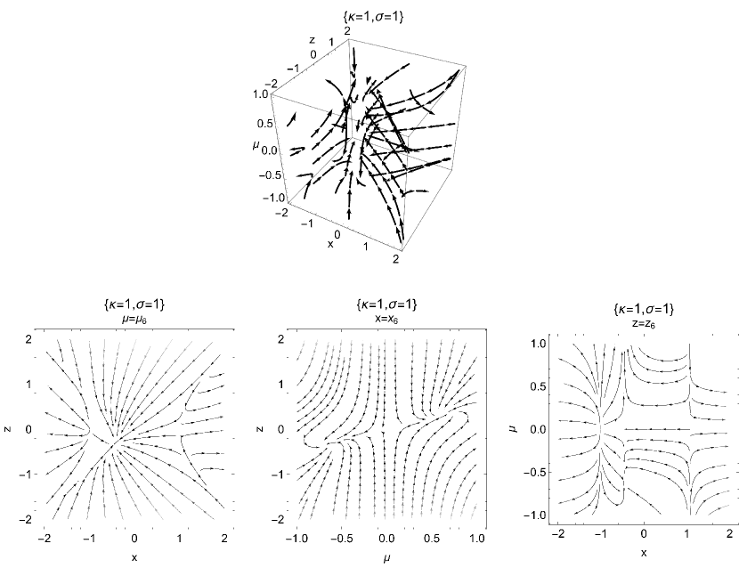
Figure 4: Phase-space portrait for the dynamical system with the mixed potential function $V\left(\phi,\psi\right)=U_{0}e^{\kappa\phi}\psi^{\frac{1}{\sigma}}$. We observe that the stationary points $A_{3}^{-}$ is an attractor.

We conclude that this model can describe a cosmological history, with an early acceleration phase (point $A_{5}$), a matter era (points $A_{2}^{\pm}$) and a future acceleration point (points $A_{3}^{\pm}$ or $A_{4}^{\pm}$).

To ensure a thorough analysis, it is imperative to study the existence of stationary points at the infinity regime.

V.2 Stationary points at the infinity

We introduce the new set of Poincare variables

$$x=\frac{X}{\bar{\rho}}~{},~{}z=\frac{Z}{\bar{\rho}}\text{~{}},~{}d\bar{T}=\bar{\rho}d\tau.$$

where now $\rho=\sqrt{1-X^{2}-Z^{2}}~{}$and we have used the constraint condition $u=\sqrt{1-x^{2}+z^{2}}$.

Therefore, the field equations in the Poincare variables $\left(X,Z\right)$ read

$$\frac{dX}{d\bar{T}}=\frac{1}{2}\left(1-2X^{2}\right)\left(\sqrt{6}\kappa\left(X^{2}-1-Z^{2}\right)-6X\bar{\rho}-\sqrt{6}XZ\mu\right),$$ (41)

$$\frac{dZ}{d\bar{T}}=3Z\bar{\rho}\left(2X^{2}-1\right)+\sqrt{6}\kappa\left(Z^{2}-X^{2}\right)+\frac{\sqrt{6}}{2}\mu\left(1-2X^{2}\right)\left(1-Z^{2}\right),$$ (42)

and

$$\frac{d\mu}{d\bar{T}}=-\frac{\sqrt{6}}{2}\mu\left(\kappa X+2\sigma\mu Z\right).$$ (43)

The stationary points of the aforementioned dynamical system are of the form $B=\left(X\left(B\right),Z\left(B\right),\mu\left(B\right)\right)$; they are

$$B_{1}^{\pm}=\left(\pm 1,0,0\right)~{},$$

$$B_{2}^{\pm}=\left(\frac{\sqrt{2}}{2},\pm\frac{\sqrt{2}}{2},0\right)~{},$$

$$B_{3}^{\pm}=\left(-\frac{\sqrt{2}}{2},\pm\frac{\sqrt{2}}{2},0\right)~{},$$

$$B_{4}^{\pm}=\left(\frac{\sqrt{2}}{2},\pm\frac{\sqrt{2}}{2},\mp\frac{\kappa}{2\sigma}\right),$$

$$B_{5}^{\pm}=\left(-\frac{\sqrt{2}}{2},\pm\frac{\sqrt{2}}{2},\pm\frac{\kappa}{2\sigma}\right),$$

$$B_{6}^{\pm}=\left(\sqrt{\frac{4\sigma}{1+4\sigma}},\pm\sqrt{\frac{1}{1+4\sigma}},\mp\frac{\kappa}{\sqrt{\sigma}}\right)~{},$$

$$B_{7}^{\pm}=\left(-\sqrt{\frac{4\sigma}{1+4\sigma}},\pm\sqrt{\frac{1}{1+4\sigma}},\pm\frac{\kappa}{\sqrt{\sigma}}\right)~{}.$$

Points $B_{1}^{\pm}$ are not physically accepted, while points $B_{6}^{\pm}$ and $B_{7}^{\pm}$ are real for $0<\sigma<\frac{1}{4}\,$.

Regarding the physical properties of the stationary points $B_{2}^{\pm}$, $B_{3}^{\pm}$, $B_{4}^{\pm}$ and $B_{5}^{\pm},$ the points describe dust fluid asymptotic solutions; on the other hand, points $B_{6}^{\pm}$ and $B_{7}^{\pm}$ correspond to Big Rip singularities.

The eigenvalues of the linearized system around the stationary points $B_{2}^{\pm}$ and $B_{3}^{\pm}$ are $e_{1}\left(B_{2}^{\pm}\right)=-\frac{\sqrt{3}}{2}\kappa,~{}e_{2}\left(B_{2}^{\pm}\right)=\sqrt{3}\kappa~{}$, $e_{3}\left(B_{2}^{\pm}\right)=2\sqrt{3}\kappa$ and $e_{1}\left(B_{3}^{\pm}\right)=\frac{\sqrt{3}}{2}\kappa,~{}e_{2}\left(B_{3}^{\pm}\right)=-\sqrt{3}\kappa~{}$, $e_{3}\left(B_{3}^{\pm}\right)=-2\sqrt{3}\kappa$ respectively. Hence, these two sets of points are always saddle points. Furthermore, for the points $B_{4}^{\pm}$ and $B_{5}^{\pm}$ we derive the eigenvalues $e_{1}\left(B_{4}^{\pm}\right)=-\frac{\sqrt{3}\kappa\left(1-4\sigma\right)}{2\sigma}\kappa,~{}e_{2}\left(B_{4}^{\pm}\right)=\sqrt{3}\kappa~{}$, $e_{3}\left(B_{4}^{\pm}\right)=2\sqrt{3}\kappa$ and $e_{1}\left(B_{5}^{\pm}\right)=\frac{\sqrt{3}\kappa\left(1-4\sigma\right)}{2\sigma}\kappa,~{}e_{2}\left(B_{5}^{\pm}\right)=-\sqrt{3}\kappa~{}$, $e_{3}\left(B_{5}^{\pm}\right)=-2\sqrt{3}\kappa$. Therefore, points $B_{4}^{\pm}$ are attractors for $\left\{\kappa<0,\sigma<0\text{,}\sigma>\frac{1}{4}\right\}$ while points $B_{5}^{\pm}$ are attractors for $\left\{\kappa>0,0<\sigma<\frac{1}{4}\right\}$.

Finally, the stability properties for the points $B_{6}^{\pm}$ and $B_{7}^{\pm}$ have been studied numerically. Based on our findings, we conclude that the asymptotic solutions associated with these points are consistently unstable.

The qualitative evolution of the effective equation of state parameter for this model is presented in Fig. 5.

Figure 5: Qualitative evolution of the equation of state parameter $w_{tot}\left(X,Z\right)$ as it is given by numerical simulations of the dynamical system (41)-(43) for various values of the free parameters. Left Fig. is for the initial conditions $\left(X_{0},Z_{0},\mu_{0}\right)=\left(0.6,0.1,2\right)$ while right Fig. is for the initial conditions $\left(X_{0},Z_{0},\mu_{0}\right)=\left(0.7,0.2,-2\right)$.

VI Conclusions

The Chiral model is a multi-scalar field cosmological scenario which has been proposed to describe inflation. In particular the inflationary mechanism generated by the Chiral model is known as hyperbolic inflation. In this study we considered the Chiral-quintom model which is a generalization where one of the scalar fields has phantom energy component. As a result, the hyperbolic inflationary mechanism is generalized where now the equation of state parameter can cross the phantom divide line.

Considering a spatially flat FLRW geometry within this model, we introduced a mixed potential term to modify the dynamics of the Chiral-quintom fluid. Through a comprehensive analysis of the phase-space of the field equations, we successfully reconstructed the complete cosmological history provided by this model. Remarkably, this new multi-scalar field model effectively replicates cosmological epochs that encompass the early-time and the late-time acceleration phases of the universe as well as the matter-dominated epoch. Consequently, this two-scalar field model holds promise as a unification framework for the dark sector of the universe. We remark that the cosmological history obtained from the same model without the mixed potential term dn8 can be considered a special case of this more general model

In a forthcoming study, we plan to exploer the dynamical evolution of perturbations within this multi-scalar field model featuring the mixed potential. Additionally, we find it particularly intriguing to investigate whether Chiral models can offer potential solutions to reconcile cosmological tensions that exist in current observations and measurements.

Data Availability Statements: Data sharing is not applicable to this article as no datasets were generated or analyzed during the current study.

References

• (1) Z.-K. Guo, X.-M. Zhang and Y.-Z. Zhang, Cosmological evolution of a quintom model of dark energy, Phys. Lett B 608, 177 (2005)
• (2) X. Zhang, An interacting two-fluid scenario for quintom dark energy, Comm. Theor. Phys. 44, 762 (2005)
• (3) W. Zhao, Quintom models with an equation of state crossing -1, Phys. Rev. D 73, 123509 (2006)
• (4) P. Ratra and L. Peebles, Cosmological consequences of a rolling homogeneous scalar field, Phys. Rev. D 37, 3406 (1988)
• (5) C. Wetterich, Cosmology and the fate of dilatation symmetry, Nucl. Phys. B 302, 668 (1988)
• (6) R.R. Caldwell, A Phantom Menace Cosmological consequences of a dark energy component with super-negative equation of state, Phys. Lett. B 545, 23 (2002)
• (7) F. Briscese, E. Elizalde, S. Nojiri and S.D. Odintsov, Phantom scalar dark energy as modified gravity: Understanding the origin of the Big Rip singularity, Phys. Lett. B 646, 105 (2007)
• (8) A.D. Linde, Chaotic inflation, Phys. Lett. B 129, 177 (1983)
• (9) J.D. Barrow and P. Parsons, Inflationary models with logarithmic potentials, Phys. Rev. D 52, 5576 (1995)
• (10) I. Zlatev, L. Wang and P.J. Steinhardt, Phys. Rev. Lett. 82, 896 (1999)
• (11) W. Liu, J. Ouynag and H. Yang, Quintessence Field as a Perfect Cosmic Fluid of Constant Pressure, Commun. Theor. Phys. 63, 391 (2015)
• (12) M.C. Bento, O. Bertolami and A.A. Sen, Phys. Rev. D 70, 083519 (2004)
• (13) S. Basilakos, G. Lukes-Gerakopoulos, Dynamics and constraints of the Unified Dark Matter flat cosmologies, Phys. Rev. D 78, 083509 (2008)
• (14) Planck Collaboration: N. Aghanim et al., Planck 2018 results. VI. Cosmological parameters, A&A 641, A6 (2020)
• (15) R.C. Caldwell, M. Kamionkowski and N.N. Weinberg, Phantom Energy and Cosmic Doomsday, Phys. Rev. Lett. 91, 071301 (2003)
• (16) V. Faraoni, Phantom cosmology with general potentials, Class. Quantum Grav. 22, 3235 (2005)
• (17) Y.F. Cai, E.N. Saridakis, M.R. Setare and J.Q. Xia, Quintom Cosmology: Theoretical implications and observations, Phys. Rept. 493, 1 (2010)
• (18) M.R. Setare and E.N. Saridakis, Quintom Cosmology with General Potentials, Int. J. Mod. Phys. D 18, 549 (2009)
• (19) G. Leon, Y. Leyva and J. Socorro, Quintom phase-space: beyond the exponential potential, Phys. Lett. B 732, 285 (2014)
• (20) S. Papanich, P. Burikham, S. Ponglertsakul and L. Tannukij, Resolving Hubble tension with quintom dark energy model, Chinese Physics C 45, 015108 (2021)
• (21) M. Alimohammadi and H. Mohseni Sadjadi, The w = -1 crossing of the quintom model with arbitrary potential, Phys. Lett. B 648, 113 (2007)
• (22) M.R. Setare and E.N. Saridakis, Quintom dark energy models with nearly flat potentials, Phys. Rev. D 79, 043005 (2009)
• (23) J. Sadeghi, The deformation of quintom dark energy model, Astrophys. Space Sci. 364, 64 (2019)
• (24) R. Lazkoz, G. Leon and I. Quiros, Quintom cosmologies with arbitrary potentials, Phys. Lett. B 649, 103 (2007)
• (25) J. Socorro, S. Perez-Payan, A. Espinoza-Garcia and L.R. Diaz-Barron, Quintom Fields from Chiral K-Essence Cosmology, Universe 8, 548 (2022)
• (26) J. Socorro, P. Romero, L.O. Pimentel and M. Aguero, Quintom potentials from quantum cosmology using the FRW cosmological model, Int. J. Theor. Phys. 52, 2722 (2013)
• (27) G. Leon and A. Paliathanasis, The past and future dynamics of quintom dark energy models, Eur. Phys. J. C 78, 753 (2018)
• (28) J.A. Vázquez, D. Tamayo,G. Garcia-Arroyo, I. Gómez-Vargas, I. Quiros and A.A. Sen, Coupled Multi Scalar Field Dark Energy, (2023) [arXiv:2305.11396]
• (29) M.R Setare and M. Saharaee, Gen. Relativ. Grav. 48., 119 (2016)
• (30) M. Marciu, Dynamical description of a quintom cosmological model nonminimally coupled with gravity, Eur. Phys. J. C 80, 894 (2020)
• (31) M. Marciu, Quintom Cosmology with Generalized Galileon Corrections, Rom. J. Phys. 65, 115 (2020)
• (32) K.F. Dialektopoulos, G. Leon and A. Paliathanasis, Multiscalar-torsion cosmology: exact and analytic solutions from noether symmetries, Eur. Phys. J. C 83, 218 (2023)
• (33) M. Marciu, Prospects of the cosmic scenery in a quintom dark energy model with generalized nonminimal Gauss-Bonnet couplings, Phys. Rev. D 99, 043508 (2019)
• (34) S. V. Ketov, Quantum Non-linear Sigma Models, Springer-Verlag, Berlin, (2000).
• (35) S.V. Chervon, Chiral Cosmological Models: Dark Sector Fields Description, Quantum Matter 2, 71 (2013)
• (36) I.V. Fomin, The chiral cosmological models with two components, J. Phys.: Conf. Ser. 918, 012009 (2017)
• (37) A. R. Brown, Hyperbolic Inflation, Phys. Rev. Lett. 121, 251601 (2018)
• (38) P. Christodoulidis, D. Roest and R. Rosati, Many-field Inflation: Universality or Prior Dependence?, JCAP 04, 021 (2020)
• (39) D.H. Lyth, A numerical study of non-gaussianity in the curvaton scenario, JCAP 6, 511, (2005)
• (40) D. Langlois and S. Renaux-Peterl, Perturbations in generalized multi-field inflation, JCAP 17, 804 (2008)
• (41) A. Paliathanasis and M. Tsamparlis, Two scalar field cosmology: Conservation laws and exact solutions, Phys. Rev. D 90, 043529 (2014)
• (42) N. Dimakis, A. Paliathanasis, P.A. Terzis and T. Christodoulakis, Cosmological solutions in multiscalar field theory, EPJC 79, 618 (2019)
• (43) P. Christodoulidis, D. Roest and E.I. Sfakianakis, Attractors, bifurcations and curvature in multi-field inflation, JCAP 08, 006 (2020)
• (44) A. Paliathanasis, Dynamics of Chiral Cosmology, Class. Quantum Grav. 37, 19 (2020)
• (45) N. Dimakis and A. Paliathanasis, Crossing the phantom divide line as an effect of quantum transitions, Class. Quantum Grav. 38, 075016 (2021)
• (46) P. Christodoulidis and A. Paliathanasis, N-field cosmology in hyperbolic field space: stability and general solutions, JCAP 05, 038 (2021)
• (47) P. Christodoulidis and R. Rosati, (Slow-)Twisting inflationary attractors, (2022) [arXiv:2210.14900]
• (48) A. Paliathanasis and G. Leon, Hyperbolic inflationary model with nonzero curvature, Phys. Lett. B 834, 137407 (2022)
• (49) A. Paliathanasis and G. Leon, Dynamics of a two scalar field cosmological model with phantom terms, Class. Quantum Grav. 38, 075013 (2021)
• (50) A. Paliathanasis and G. Leon, Global dynamics of the hyperbolic Chiral-Phantom model, Eur. Phys. J. Plus 137, 165 (2022)
• (51) J. Tot, B. Yildirim, A. Coley and G. Leon, The dynamics of scalar-field Quintom cosmological models, Phys. Dark Univ. 39, 101155 (2023)
• (52) E.J. Copeland, A.R. Liddle and D. Wands, Exponential potentials and cosmological scaling solutions, Phys. Rev. D 57, 4686 (1998)