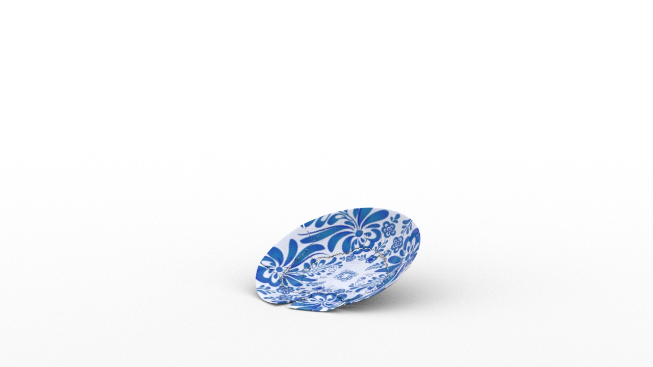
Figure 1. Our simulation depicts a cracked ceramic plate, resulting from a forceful impact with a hard surface. With our method, we were able to simulate this complex scene using mere 600K particles. Our approach has demonstrated a 3x speed improvement over the current state-of-the-art method.

Variational Bonded Discrete Element Method with Manifold Optimization

Abstract.

This paper proposes a novel approach that combines variational integration with the bonded discrete element method (BDEM) to achieve faster and more accurate fracture simulations. The approach leverages the efficiency of implicit integration and the accuracy of BDEM in modeling fracture phenomena. We introduce a variational integrator and a manifold optimization approach utilizing a nullspace operator to speed up the solving of quaternion-constrained systems. Additionally, the paper presents an element packing and surface reconstruction method specifically designed for bonded discrete element methods. Results from the experiments prove that the proposed method offers 2.8 to 12 times faster state-of-the-art methods.

1. Introduction

Fracture simulation is a topic of great importance in the field of physically-based simulations, as it represents a fundamental type of interaction within virtual environments. However, simulating fractures is a complex task due to the omnipresence of fractures in the real world and the need for accurate representation to provide a sense of realism. Most simulation methods are based on continuum theory, which can be limiting when it comes to accounting for fracture phenomena. While the bonded discrete element method can better simulate fractures, the time cost associated with this method can be a significant obstacle that hinders its adoption.

One of the most significant challenges in fracture simulation is achieving accurate measurements of internal forces while allowing for an acceptable error rate in fracture propagation. At this stage of simulation, numerical methods become critical in overcoming these challenges. Specifically, solving BDEM systems is complicated by the stiff nature of unit length constraint in quaternion systems, and the added complexities of shear stiffness in materials such as rope or cloth. Additionally, collision stiffness in discrete element simulations can lead to significant complications in solving the system, increasing the number of Newton iterations required. These issues are prevalent in different simulation approaches.

To address these challenges, we propose an approach that combines variational integrator with BDEM that can deliver faster and more accurate simulations. Our approach leverages the advantages of BDEM to more accurately model fracture phenomena while simultaneously taking advantage of the computational efficiencies inherent in implicit integration to achieve faster simulations.

In this paper, we describe the implementation of our new approach, present experimental results, and compare our performance to current state-of-the-art methods. Our experiments show that the proposed approach is more efficient than current state-of-the-art methods. Our contributions include:

• a variational formulation and a manifold optimization approach that involves a nullspace operator, which speeds up the solving of quaternion-constrained systems.

• a stable integrator suitable for implicit bonded discrete element methods with large time steps.

• an element packing and surface reconstruction method specifically designed for bonded discrete element methods.

2. Related Works

Discrete Element Method

The Discrete Element Method (DEM) has been widely adopted in engineering for simulating granular materials, after being introduced by Cundall and Strack for rock mechanics (Cundall, 1971; Cundall and Strack, 1979). DEM has also been applied in computer graphics to simulate granular materials (Bell et al., 2005; Alduán et al., 2009; Rungjiratananon et al., 2008; Yue et al., 2018). Recent work by De Smedt et al. (De Klerk et al., 2022) used a variational integrator to model the contact between granular materials. To extend the use of DEM to simulate continuum media, BDEM was introduced (Potyondy and Cundall, 2004), which has been successful in many engineering applications where classical models fail or become too computationally expensive. Andre et al. (André et al., 2012) used a cohesive bond model to model continuum objects, while Nguyen et al. (Nguyen et al., 2021) added a plastic cohesive bond to simulate ductile fractures. BDEM has also been recently introduced to the computer graphics community for simulating realistic fractures (Lu et al., 2021). While BDEM shows potential for simulating fractures realistically, the computational cost is high due to the need for small time steps.

The Discrete Element Method (DEM), originally introduced by Cundall and Strack for rock mechanics (Cundall, 1971; Cundall and Strack, 1979), is now a widely used tool for simulating granular materials in engineering. The DEM has also been applied in computer graphics for simulating granular materials (Bell et al., 2005; Alduán et al., 2009; Rungjiratananon et al., 2008; Yue et al., 2018). (De Klerk et al., 2022) used a variational integrator to model the contact between granular materials. To extend the use of the DEM in simulating continuum media, BDEM was introduced (Potyondy and Cundall, 2004), which has shown great success in many engineering applications where classical models fail or become prohibitively expensive to run. (André et al., 2012) use cohesive bond model to model continuum object. (Nguyen et al., 2021) add plastic cohesive bond to model ductile fracture. BDEM has also recently been introduced to the computer graphics community (Lu et al., 2021). Although BDEM demonstrates potential in simulating realistic fractures, the time cost is currently high due to the need for small time steps.

Simulation with Orient or Rotation

Researchers have explored methods for simulating objects with orientational or rotational degrees of freedom, beyond DEM. One such method uses particles with orientation, as discussed in (Müller and Chentanez, 2011). However, this geometric approach lacks physical concepts such as momentum and stress, which can limit its ability to provide physically accurate effects.

To enable more detailed simulations of specific structures, researchers have explored the use of rod elements. For example, the Discrete Differential Geometry (DDG) approach in (Bergou et al., 2008) was used to compute rod curvature, while Cosserat rods were used in (Kugelstadt and Schömer, 2016; Soler et al., 2018) to model complex bending and torsion effects. Unlike discrete elements in DEM, rod elements discretize solid objects into slender, flexible structures like ropes and fibers and are less effective at describing generic 2D or 3D objects.

Implicit Integrators

In computer graphics, implicit integrators are a commonly used tool for simulation, with backward Euler being the most prevalent method (Baraff and Witkin, 1998; Hirota et al., 2001; Volino and Magnenat-Thalmann, 2001; Martin et al., 2011; Liu et al., 2013). Other integrators, such as the implicit-explicit method (Eberhardt et al., 2000; Stern and Grinspun, 2009) and exponential integrators (Michels et al., 2014; Chen et al., 2017), have also received significant attention.

From a variational perspective, integrators with an optimization view (Gast et al., 2015) have yielded promising results, as they transform simulations into nonlinear optimization problems. Optimization-based integrators have been used to tackle various simulation problems, such as crowd simulations (Karamouzas et al., 2017), large-step simulation of deformable objects with nonlinear material (Li et al., 2019), and simulation of hyperelastic solids using SPH (Kee et al., 2023). Hierarchical optimization time integration in MPM (Wang et al., 2020) and higher-order integration for deformable solids simulation with stiff, nonlinear material and contact handling (Löschner et al., 2020) have also been proposed. Additionally, some techniques propose a blend between implicit mid-point and forward/backward Euler to preserve energy and maintain stable integration (Dinev et al., 2018).

Variational integrators (VIs) have emerged as a promising tool for the simulation of diverse phenomena in computer graphics, such as deformable objects, cloth, fluids, and rigid bodies (Trusty et al., 2022; Thomaszewski et al., 2008; Batty et al., 2012; Alduán et al., 2009). The use of VIs ensures good long-term stability and energy conservation. Moreover, the variational framework underlying VIs allows for a flexible and intuitive description of constraints and system dynamics(Kane et al., 2000; Kharevych et al., 2006; Lew and Mata A, 2016), which is particularly useful for interactive applications and artistic control. Studies have demonstrated the effectiveness of VIs for specific applications, such as cloth simulation using asynchronous variational integrators (Thomaszewski et al., 2008), contact mechanics using asynchronous variational integrators (Harmon et al., 2009), and scalable simulation of generic mechanical systems using VIs (Alduán et al., 2009). Additionally, research has explored the use of VIs in optimal control (Johnson et al., 2014), fluid simulation using discrete Lagrangians (Batty et al., 2012), variational networks (Saemundsson et al., 2020), and mixed finite element methods for simulation of deformable objects (Trusty et al., 2022).

Fracture Simulation

In the field of computer graphics, fracture simulation is a significant research topic. Non-physical methods have been proposed to produce crack patterns (Raghavachary, 2002; Hellrung et al., 2009; Su et al., 2009; Bao et al., 2007; Zheng and James, 2010; Schvartzman and Otaduy, 2014; Müller et al., 2013). However, physics-based approaches are more accurate and preferred for fracture simulation. Finite element method (FEM) is a widely used physics-based technique for fracture simulation (O’Brien and Hodgins, 1999; Müller et al., 2001; Wicke et al., 2010; Koschier et al., 2014; Pfaff et al., 2014). Extended finite element method (XFEM)(Kaufmann et al., 2009; Chitalu et al., 2020), boundary element method (BEM) (Hahn and Wojtan, 2015, 2016; Zhu et al., 2015), meshless method (Pauly et al., 2005), peridynamics (Chen et al., 2018), and material point method (MPM) (Wolper et al., 2019; Joshuah et al., 2020) are other physics-based techniques used for fracture simulation. Each of these methods has its own pros and cons and is suitable for different fracture scenarios.

In the context of fracture simulation, accurately representing the fracture surface is essential due to the complicated nature of fracture propagation. When utilizing FEM, remeshing techniques are often employed in order to prevent the creation of sharp elements, which can lead to numerical instability and other issues (Chen et al., 2014; Koschier et al., 2014; Pfaff et al., 2014; Wicke et al., 2010). Additional methods for FEM-based fracture simulation include the use of duplicate elements (Molino et al., 2004) or sub-elements (Nesme et al., 2009; Wojtan and Turk, 2008). Explicit surface methods can be used to more effectively track the fracture surface and improve the accuracy of the simulation (Koschier et al., 2017). Post-processing techniques may also be used to add further details and improve the quality of the simulation results (Chitalu et al., 2020; Kaufmann et al., 2009). Level set methods may also be leveraged to more accurately represent the geometry of the fracture surface (Hahn and Wojtan, 2015). Alternatively, mesh-based methods can be used directly to represent manifold crack surfaces (Chitalu et al., 2020; Sifakis et al., 2007; Zhu et al., 2015). Accurately representing fracture surfaces remains a challenging task, as each approach to representation has its own advantages and disadvantages, and selecting the most appropriate method depends on the specific needs of the simulation.

3. Quaternion for Rotation

A quaternion can be represented in the following form,

(1) $$q=ui+vj+wk+s=\{u,v,w,s\}=\begin{pmatrix}u\\ v\\ w\\ s\end{pmatrix}$$

A unit quaternion can correspond to a rotation in three-dimensional space. Quaternions are widely used in computer graphics to represent rotation due to their computational simplicity and efficiency when compared to other rotation representations such as Euler angles, axis-angle, or rotation matrices. In BDEM, the state of a discrete element includes both displacement and rotation, with quaternions commonly used to represent the rotation status of the element. Quaternions are extremely important in implicit methods based on BDEM and their acceleration. In the following chapters, many quaternion-related operations will be utilized. To aid the reader’s understanding, we have listed some key information related to quaternion operations.

Quaternion Multiplication

The multiplication of quaternions represents the composition of rotations. Left multiplication of quaternions represents the order of rotation, while right multiplication of quaternions represents the rotation of the coordinate system afterwards. Rotations using quaternions can also be represented in matrix form, where $Q_{l}(q)$ is called the left multiplication matrix and $Q_{r}(q)$ is called the right multiplication matrix.

(2) $$q_{i}q_{j}=Q_{l}(q_{i})q_{j}=Q_{r}(q_{j})q_{i}$$

We use vector $t$ to express the imaginary part of quaternion as $t=\{u,v,w\}$. Then, the left and right multiplication matrices can be expressed in the following way

(3) $$Q_{l}(q)=\begin{pmatrix}sI_{3}+t^{\times}&t\\ -t^{T}&s\end{pmatrix}$$

(4) $$Q_{r}(q)=\begin{pmatrix}sI_{3}-t^{\times}&t\\ -t^{T}&s\end{pmatrix}$$

The skew symmetric matrix $t^{\times}$ is cross matrix for vector $t$

(5) $$t^{\times}=\begin{pmatrix}0&-w&v\\ w&0&-u\\ -v&u&0\end{pmatrix}$$

Spatial Rotation with Quaternion

For a direction $d_{0}$ in 3d space, with a rotation expressed by quaternion $q$, the rotated new direction $d$ can be calculated by

(6) $$\begin{pmatrix}d\\ 0\end{pmatrix}=q\begin{pmatrix}d_{0}\\ 0\end{pmatrix}\overline{q}$$

where $\overline{q}$ is the conjugate of quaternion, defined as $\overline{q}=\{-u,-v,-w,s\}$. It has the property that composition of quaternion and conjugate is the unit quaternion as $\overline{q}q=\{0,0,0,1\}$. In the latter chapters, we use $\odot$ to stand for the direction rotation operator with $d=q\odot d_{0}$.

Nullspace Operator

We can rewrite the composition of quaternion and its conjugate in matrix form,

(7) $$\overline{q}q=Q_{l}(\overline{q})q=\begin{pmatrix}sI_{3}-t^{\times}&-t\\ t^{T}&s\end{pmatrix}\begin{pmatrix}t\\ s\end{pmatrix}=\begin{pmatrix}0\\ 0\\ 0\\ 1\end{pmatrix}$$

Noting that by taking only the upper half of the matrix, we can obtain a null space operation matrix for quaternions. We can define the upper matrix of $Q_{l}(\overline{q})$ as

(8) $$G_{l}(q)=\begin{pmatrix}sI_{3}-t^{\times}&-t\end{pmatrix},G_{r}(q)=\begin{pmatrix}sI_{3}+t^{\times}&-t\end{pmatrix}$$

It has the properties that

(9) $$G_{l}(q)q=0,G_{r}(q)q=0$$

As $G_{l}(q_{i})q_{j}$ remove the componenet of $q_{i}$ in $q_{j}$ and project the vector to the direction of angle axis of quaternion $\overline{q_{i}}q_{j}$, it has many usefull applications. We can also relate the quaternion matrix with nullspace oprator matrix as

(10) $$Q_{l}(q)=\begin{pmatrix}G_{l}(q)^{T}&q\end{pmatrix},Q_{r}(q)=\begin{pmatrix}G_{r}(q)^{T}&q\end{pmatrix}$$

.

Derivation and Angular Velocity

We can extend the angular velocity to four dimensions in the following way

(11) $$w_{4}=\begin{pmatrix}w\\ 0\\ \end{pmatrix}$$

There is a relationship between the derivative of quaternions and extened angular velocity in the following form (Betsch and Siebert, 2009):

(12) $$\dot{q}=\frac{1}{2}w_{4}q$$

(13) $$w_{4}=2\dot{q}\overline{q}$$

Quaternion Constraint

A rotation in space can be represented by a unit quaternion. To ensure that the quaternion stays unit during calculation, constraints must be imposed on its modulus length

(14) $$C(q)=\frac{1}{2}(q^{T}q-1)=0$$

4. Variational Bonded Discrete Element Method

One significant difference between bonded discrete element method and other approaches is the direct consideration of rotation Degrees of Freedom (DoFs) as system variables. Previous methods solve bonded discrete element systems using explicit formulations that store rotation status as quaternion, Euler angles, or axis angle and compute torques and angular velocities explicitly to alter the rotation status or the discrete element. In implicit formulations, deltas of position or rotation status are unknowns, while forces or torques are often implicit or invisible during system solving. Consequently, a new formulation is required to describe the momentum equation with quaternion representation. In this study, we utilized discretized Hamilton’s principle to derive the variational integrator form of the bonded discrete element method. With this new equation form, an implicit integrator can be easily derived, making this method not only suitable for bonded discrete element method but also for any quaternion-based rotation system. Here, we introduce the discrete Hamilton’s principle and derive the new variational integrator form of dynamics with rotation.

4.1. Variational Implicit Integrators

Hamilton’s principle

Hamilton’s Principle, a fundamental principle in physics, can be used to derive the equations of motion for a physical system. By varying the Lagrangian functional, which takes the form of an integral of the Lagrangian function over time as $S=\int_{t_{0}}^{t_{1}}L(x,\dot{x},t)dt$, the equations of motion can be obtained as the stationary point of the action functional. For our system, the Lagrangian function is given as the sum of kinetic and potential energy terms,

(15) $$L=T-V=\frac{1}{2}\dot{x}^{T}M\dot{x}-V(x)$$

Using this Lagrangian function, the true evolution of the physical system is the solution of $\frac{\partial{S}}{\partial{x(t)}}=0$.

Discrete Lagrangian

To approximate the action functional in a small time interval, a discrete Lagrangian is used.

(16) $$S_{d}=\sum_{t_{i}=t_{0}}^{t_{n-1}}L_{d}(t_{i},t_{i+1},x_{i},x_{i+1})\approx\int_{t_{0}}^{t_{n}}L(t,x(t))dt$$

In the stationary point of the discrete action functional, each term of the sum must be set to zero.

(17) $$\frac{\partial{S_{d}}}{\partial{x_{i}}}=0=\frac{\partial L_{d}(t_{i-1},t_{i},x_{i-1},x_{i})}{\partial x_{i}}+\frac{\partial L_{d}(t_{i},t_{i+1},x_{i},x_{i+1})}{\partial x_{i}}$$

A variational integrator can then be derived using discrete Hamilton’s Principle. We can use a fixed time step $\Delta t$ and a linear approximation of velocity to approximate the kinetic energy term as in the discrete Lagrangian.

(18) $$\int_{t_{0}}^{t_{n}}Tdt\approx\sum_{t_{i}=t_{0}}^{t_{n-1}}\Delta t\frac{1}{2}v_{i}^{T}Mv_{i}$$

Different approximations can be selected for the potential energy term to obtain different forms of variational integrators.

Mid-Point Approximation

If the Lagrangian integral is approximated by taking the mid-point as

(19) $$L_{d}(t_{i},t_{i+1},x_{i},x_{i+1})=\Delta t\frac{1}{2}v_{i}^{T}Mv_{i}-\Delta tV(\frac{x_{i+1}+x_{i}}{2})$$

according to equation(17),

(20) $$\frac{\partial L_{d}(t_{i-1},t_{i},x_{i-1},x_{i})}{\partial x_{i}}=\frac{1}{\Delta t}M(x_{i}-x_{i-1})-\frac{1}{2}\Delta t\nabla V(\frac{x_{x-1}+x_{i}}{2})$$

(21) $$\frac{\partial L_{d}(t_{i},t_{i+1},x_{i},x_{i+1})}{\partial x_{i}}=\frac{1}{\Delta t}M(x_{i+1}-x_{i})+\frac{1}{2}\Delta t\nabla V(\frac{x_{i}+x_{i+1}}{2})$$

let $\hat{x}=2x_{i}-x_{i-1}$, we can get the mid-point form of variational integrator

(22) $$\frac{1}{\Delta t^{2}}M(x_{i+1}-\hat{x})+\frac{1}{2}\nabla V(\frac{x_{i+1}+x_{i}}{2})+\frac{1}{2}\nabla V(\frac{x_{i-1}+x_{i}}{2})=0$$

Left-Point Approximation

If we use left-point to approxmate the potential term as

(23) $$V_{d}(t_{i},t_{i+1},x_{i},x_{i+1})=\Delta tV(x_{i})$$

we can obtain a left-point integrator

(24) $$\frac{1}{\Delta t^{2}}M(x_{i+1}-\hat{x})+\nabla V(x_{i})=0$$

Right-Point Gradient Approximation

We can use the right-point gradient to approxmiate the potential term

(25) $$V_{d}(t_{i},t_{i+1},x_{i},x_{i+1})=\Delta t(V(x_{i+1})-\nabla V(x_{i+1})\frac{x_{i+1}-x_{i}}{2})$$

(26) $$V_{d}(t_{i-1},t_{i},x_{i-1},x_{i})=\Delta t(V(x_{i-1})+\nabla V(x_{i+1})\frac{x_{i}-x_{i-1}}{2})$$

we can obtain a right-point integrator

(27) $$\frac{1}{\Delta t^{2}}M(x_{i+1}-\hat{x})+\nabla V(x_{i+1})=0$$

4.2. Hamiltonian Formulation in BDEM

The key to the discrete Lagrangian formulation is defining the kinetic and potential energy of the system. For a general displacement system, the kinetic energy is defined by the mass matrix $M_{p}$ of the system and its velocity $\dot{p}$

(28) $$T_{p}=\frac{1}{2}\dot{p}^{T}M_{p}\dot{p}$$

For a rotation system, the system’s kinetic energy can be defined by angular kinetic energy but needs to be represented in quaternion form. We derive the quaternion form of kinetic energy as follows

(29) $$T_{q}=\frac{1}{2}w^{T}Jw$$

To represent it in quaternion form, we extend the moment of inertia matrix as

(30) $$J_{4}=\begin{pmatrix}J&\\ &J_{0}\\ \end{pmatrix}$$

According to Equation(13), we can obtain a new form of kinetic energy

(31) $$\begin{split}T_{q}&=\frac{1}{2}w_{4}^{T}J_{4}w_{4}\\ &=\frac{1}{2}(2\dot{q}\bar{q})^{T}J_{4}(2\dot{q}\bar{q})\\ &=\frac{1}{2}\dot{q}^{T}4Q_{r}(\bar{q})^{T}J_{4}Q_{r}(\bar{q})\dot{q}\end{split}$$

$\bar{q}$ is the conjugate of quaternion $q$, $Q_{r}(\overline{q})$ are corresponding matrix form of quaternion multiplication. By defining a equivalent mass matrix $M_{q}(q)=4Q_{r}(\bar{q})^{T}J_{4}Q_{r}(\bar{q})$, we can simplify the kinetic energy form to

(32) $$T_{q}=\frac{1}{2}\dot{q}^{T}M_{q}(q)\dot{q}$$

4.2.1. Kinetic Energy in BDEM

To facilitate calculations in BDEM simulations, we commonly employ spherical discrete elements. For a sphere with mass $m$ and radius $r$, the mass matrix can be expressed as $M_{p}=mI_{3}$, while its moment of inertia takes a value of $J=\frac{2}{5}mr^{2}I_{3}$. Because the choice of $J_{0}$ does not impact the actual magnitude of kinetic energy, we set it as $\frac{2}{5}mr^{2}$. Consequently, the equivalent rotational mass matrix can be written in the following manner

(33) $$M_{q}(q)=4Q_{r}(\bar{q})^{T}J_{4}Q_{r}(\bar{q})=\frac{8}{5}mr^{2}Q_{r}(\bar{q})^{T}Q_{r}(\bar{q})=\frac{8}{5}mr^{2}I_{4}$$

If we define the state of the spherical elements as $x=\{p,q\}$, then we can express the kinetic energy of the elements using the following equation:

(34) $$T=\frac{1}{2}\dot{x}^{T}M_{s}\dot{x}$$

where $M_{s}$ is the Equivalent mass matrix

(35) $$M_{s}=\begin{pmatrix}M_{p}&\\ &M_{q}\end{pmatrix}$$

4.2.2. Potential Energy in BDEM

In a setup where two vertices with positions $p_{i}$ and $p_{j}$ are bonded together, along with their respective rotations $q_{i}$ and $q_{j}$, the deformation of the bond can be decomposed into four forms: stretch, shear, bend, and twist, akin to the form presented in (Lu et al., 2021). It is straightforward to derive the bond energy with these four deformation types, which can be expressed as follows:

(36) $$V=V_{\mbox{stretch}}+V_{\mbox{shear}}+V_{\mbox{bendtwist}}$$

Stretch

The stretch energy of a bond can be modeled using a simple spring model and expressed as follows:

(37) $$V_{\mbox{stretch}}=\frac{1}{2}k_{n}\|p_{i}-p_{j}\|^{2}$$

$k_{n}=ES/l_{0}$ is the stretch stiffness, $E$ represents Young’s modulus, $S=\pi r^{2}$ is the cross-sectional area of bond, and $l_{0}$ is the bond’s restlength.

Shear

The article (Lu et al., 2021) explains that shear energy can be defined as the difference between the common rotational component of discrete elements and the initial frame. To extract the common rotation, the equation $q_{c}=(q_{i}+q_{j})/\|q_{i}+q_{j}\|$ is used, where $d=q_{c}\odot d_{0}$ represents the current direction. The corresponding energy can be expressed as

(38) $$V_{\mbox{shear}}=\frac{1}{2}k_{t}\theta^{2}$$

where $\theta=\left<d_{0},d_{q}\right>$ denotes the angle between the bond’s initial direction $d_{0}$ and current direction $d$. The shear stiffness, $k_{t}=GS/l_{0}$, where $G$ represents the material’s shear modulus.

Bend and Twist

The bend and twist energy of discrete elements can be defined as the difference in their rotational component. It is important to note that the stiffness of bend and twist have distinct relationships with material properties, thus requiring separate decomposition of the two types of rotations. The difference of quaternion, expressed in the form of $G_{l}(q_{j})q_{i}$, can be transformed to the local frame via rotation matrix $R_{0}=G_{l}(q_{0})G_{r}(q_{0})$. The resulting vector can then be represented as $t=R_{0}G_{l}(q_{j})q_{i}$. With the aid of the stretch and shear stiffness matrix denoted as $K$, the energy form can be expressed using

(39) $$V_{\mbox{bendtwist}}=\frac{1}{2}t^{T}Kt$$

The stiffness matrix is defined by

(40) $$K=\frac{1}{l_{0}}\begin{pmatrix}GJ&&\\ &EI&\\ &&EI\end{pmatrix}$$

Here, $I=\pi r_{0}^{4}/4$ and $J=\pi r_{0}^{4}/2$ are the second moments of area for bending and twisting, respectively.

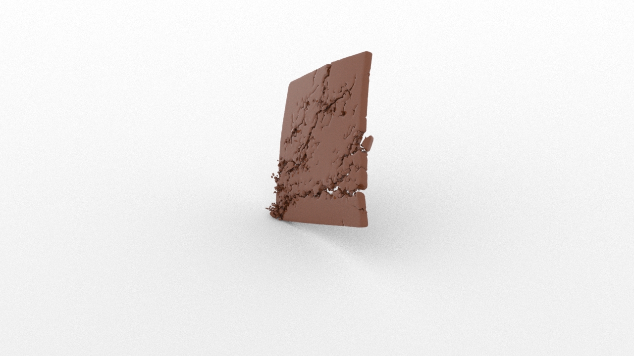
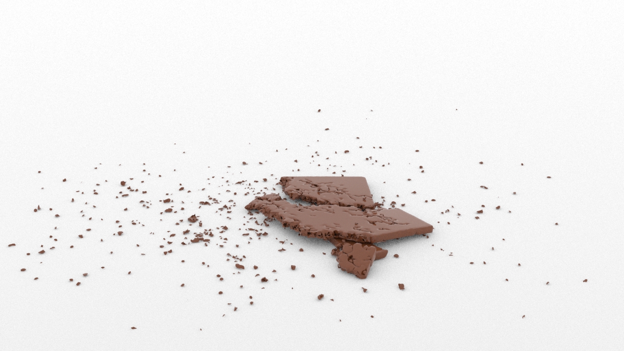
Figure 2. showcases the experimental results of our method on a chocolate drop impact simulation. The figure illustrates the moment when a chocolate drop hits the ground and cracks into several pieces and small fragments. The simulation shows the effectiveness of our approach in accurately modeling high-speed object collisions and fracture phenomena.

5. Manifold Optimization

Our implicit BDEM solver is based on a right-point integrator form expressed in Equation (27). To obtain the solution for BDEM, a new incremental potential function $\Phi(\bm{x}_{i+1})$ is introduced.

(41) $$\Phi(\bm{x}_{i+1})=\frac{1}{\Delta t^{2}}(\bm{x}_{i+1}-\hat{\bm{x}})^{T}M_{s}(\bm{x}_{i+1}-\hat{\bm{x}})+V(\bm{x}_{i+1})$$

This leads to an optimization problem formulation, where the new potential is minimized subject to the quaternion constraint $\bm{C}(\bm{x})=0$ (Equation (14)). This formulation is challenging to solve, and previous approaches like penalty method or Lagrangian multiplier methods, were found to be inefficient.

To tackle this problem, we introduce a new approach called manifold optimization, which specifically deals with the quaternion constraint and provides a more effective solution. Our research shows that the quaternion constraint can be represented as a hyper sphere, making it more suitable for searching on a manifold than complex manifolds such as collision manifolds. In the following, we discuss in depth the formulation of the BDEM problem as a constrained optimization problem and our innovative and practical approach to solving it using manifold optimization. This approach provides a more efficient and accurate solution to the BDEM system compared to previous methods.

The manifold optimization approach replaces the constrained optimization problem on $\mathbb{R}^{n}$ with an unconstrained optimization problem on a specific manifold $\mathcal{M}$. In our approach, we utilize second-order manifold optimization and employ a nullspace operator to further reduce the number of unknowns in the system, thereby facilitating the solving of quaternion-based rotation systems. To ensure a better understanding of this process, we also introduce first-order manifold optimization and compare its performance with our more advanced approach.

5.1. First-Order Manifold Optimization

The algorithm for the first-order manifold optimization is outlined in Algorithm 1, where we denote the original objective function in Euclidean space as $\bar{f}$ and in the new manifold $\mathcal{M}$ as $f$, so that $\bar{f}|{\mathcal{M}}=f$. In our case, we define $\mathcal{M}=\prod_{i=1}^{n}\mathbb{R}^{3}\otimes\mathbb{S}^{3}$, where $n$ is the number of particles. We use $p$ to refer to the $\mathbb{R}^{3}$ space and $q$ to represent the $\mathbb{S}^{3}$ space.

Algorithm 1 First-Order Manifold Optimization

0:  Initial guess $x_{0}$, termination threshold $\epsilon$

1:  while true do

2:     Compute the $\operatorname{grad}f(x_{k})$ on the manifold $\mathcal{M}$.

3:     if $\|\operatorname{grad}f(x_{k})\|<\epsilon$ then

4:        return  $x_{k}\in\mathcal{M}$

5:     end if

6:     Use descent direction $-\operatorname{grad}f(x_{k})$ with manifold line search step $\alpha$ to update $x_{k+1}\leftarrow x_{k}-\alpha\operatorname{grad}f(x_{k})$ on the manifold $\mathcal{M}$.

7:     Project $x_{k+1}$ to the manifold $\mathcal{M}$.

8:     $k\leftarrow k+1$

9:  end while

As mentioned in (Boumal, 2022), the computation of $\operatorname{grad}f$ in Line 2 involves projecting $\operatorname{grad}\bar{f}$ into the tangent space, leading to

(42) $$\operatorname{grad}_{p}f =\operatorname{grad}_{p}\bar{f}$$

(43) $$\operatorname{grad}_{q}f =(I-qq^{T})\operatorname{grad}_{q}\bar{f}$$

Line 6 involves updating the current state with a descent direction during both the line search step and the final update. To achieve this, for particle $i$, we update $q^{i}_{k}$ along a geodesic on $\mathbb{S}^{3}$ using a descent direction $\Delta{q^{i}_{k}}$, where $\Delta q^{i}_{k}$ is obtained from $\Delta x_{k}=-\alpha\operatorname{grad}_{q}f(x_{k})$. The update from $x_{k}$ to $x_{k+1}$ can be performed using the following equations:

(44) $$p^{i}_{k+1} =p^{i}_{k}+\Delta{p^{i}}$$

(45) $$q^{i}_{k+1} =q^{i}_{k}\cos\|\Delta{q^{i}_{k}}\|+\frac{\Delta{q^{i}_{k}}}{\|\Delta{q^{i}_{k}}\|}\sin\|\Delta{q^{i}_{k}}\|$$

In Line 7, the $q$ vector is guaranteed to lie on the manifold through application of a normalization step. This step can be regarded as a manifold projection, and is given by:

(46) $$q^{i}_{k}\leftarrow\frac{q^{i}_{k}}{\|q^{i}_{k}\|}$$

This ensures that $q$ satisfies the manifold constraint, allowing the optimization process to proceed effectively.

5.2. Second-Order Manifold Optimization

Our approach involves utilizing a second-order manifold optimization method that takes the Hessian and gradient of the objective function $f(x)$ on the manifold $\mathcal{M}$ into account. The steps involved in this manifold optimization are similar to those for optimization on Euclidean space and are described in Algorithm 2.

Algorithm 2 Second-Order Manifold Optimization

0:  Initial guess $x_{0}$, termination threshold $\epsilon$

1:  while true do

2:     Compute the $\operatorname{grad}f(x_{k})$ on the manifold $\mathcal{M}$.

3:     if $\|\operatorname{grad}f(x_{k})\|<\epsilon$ then

4:        return  $x_{k}\in\mathcal{M}$

5:     end if

6:     Compute $\operatorname{Hess}f(x_{k})$ on the manifold $\mathcal{M}$.

7:     Solve $(\operatorname{Hess}f(x_{k}))\Delta x=\operatorname{grad}f(x_{k})$ in tangent space $T\!\mathcal{M}$.

8:     Use descent direction $\Delta x$ with manifold line search step $\alpha$ to update $x_{k+1}\leftarrow x_{k}+\alpha\Delta x$ on the manifold $\mathcal{M}$.

9:     Project $x_{k+1}$ to the manifold $\mathcal{M}$.

10:     $k\leftarrow k+1$

11:  end while

The computation of $\operatorname{Hess}f$ in line 6 is performed using Proposition 5.8 in (Boumal, 2022). The formulas for this computation are given below:

(47) $$\operatorname{Hess}_{p_{i},p_{j}}f =\operatorname{Hess}_{p_{i},p_{j}}\bar{f}$$

(48) $$\operatorname{Hess}_{p_{i},q_{j}}f =\operatorname{Hess}_{p_{i},q_{j}}\bar{f}(I-q_{i}q_{i}^{T})$$

(49) $$\operatorname{Hess}_{q_{i},p_{j}}f =(I-q_{i}q_{i}^{T})\operatorname{Hess}_{q_{i},p_{j}}\bar{f}$$

(50) $$\operatorname{Hess}_{q_{i},q_{j}}f =(I-q_{i}q_{i}^{T})\operatorname{Hess}_{q_{i},q_{j}}\bar{f}(I-q_{i}q_{i}^{T})$$

(51) $$\quad+\begin{cases}0&i\neq j\\ -q_{i}^{T}(\operatorname{grad}_{q_{i}}\bar{f})(I-q_{i}q_{i}^{T})&i=j\end{cases}$$

The symmetric nature of $\operatorname{Hess}f$ allows us to solve the large sparse system using the commonly used preconditioned conjugate gradient method. With manifold optimization, the constrained solving is transformed into unconstrained solving. Even so, the unknowns of the system are still more than the true degrees of freedom of the system. To overcome this issue, we use the nullspace operator. We notice that both the gradient project operator $P(q)=I-qq^{T}$ and the nullspace operator $G(q)$ have the similar property that $P(q)q=0$ and $G(q)q=0$. Therefore, the original second-order solving formulation for rotation $(I-qq^{T})H(I-qq^{T})\Delta x=(I-qq^{T})b$ is reformulated as:

(52) $$G(q)^{T}G(q)H(G(q)^{T}G(q))\Delta x=G(q)^{T}G(q)b$$

By defining $y=G(q)\Delta x$ and $z=G(q)b$, the original solving is transformed to:

(53) $$G(q)HG(q)^{T}y=z$$

The solution can then be expressed as $\Delta x=G(q)^{T}y$. This approach reduces the number of unknowns in the system to the underlying degrees of freedom of the BDEM system. This reduction, in turn, leads to a decrease in the time cost of system solving. Our experiments reveal that this splitting demonstrates convergent properties equivalent to those of the original formulation.

6. Element Packing and Surface Reconstruction

Sphere elements are frequently used in discrete element simulations because of their simplicity. However, these elements are not ideal for accurately reconstructing and rendering fracture surfaces, particularly in complex fracture boundaries. In order to overcome this limitation, we propose a novel method that utilizes a new packing approach and surface reconstruction technique. With this method, we can easily obtain fracture surfaces, even in complicated fracture scenarios.

Packing

To capturing more precise fracture surface, we use a different packing with tranditional packing method in DEM simulation by dividing objects into tetrahedra, similar to other continuum-based methods like the FEM. These tetrahedras are used to calculate the element mass and tracking the fracture behavior between elements. To keep the simplicity of simulation, we still treat these tetrahedras as spheres during simulation. Surely, this could introduce inertia or momentum errors, particularly in cases where the shape of tetrahedra is sharp. Nonetheless, we have discovered that good tetrahedral packing can distribute these errors uniformly, making them appear like randomly distributed material artifacts that do not impair the macroscopic behaviors of the object. These tetrahedra can record the natural micro-structures inside objects, including the surface between elements, resulting in fracture surfaces that are natural-looking. Despite the slight randomness introduced in element packing, it is still an effective and efficient approach for modeling complex natural micro-structures within objects.

Surface Reconstruction

Our surface reconstruction algorithm consist of five steps:

1. We initiate the procedure by identifying elements with surface faces and labeling them as surface elements.

2. During the simulation, when a bond fails between two elements, we mark these components as surface elements.

3. We employ a labeling algorithm to partition the elements into connected components.

4. We then distinguish the triangles that belong to a single surface element in each connected component and mark them as the fracture surface.

5. Finally, we use the positions and rotations of each element to compute the updated positions of the tetrahedra.

Our algorithm provides a rapid and simple method for recovering the fracture surface of bonded element methods. We specifically find this approach effective in reducing the number of bonds present in a random close packing system since the maximum number of bonds per element is solely four. We have demonstrated in experiments that bonded discrete elements can produce accurate deformation results using our technique.

Table 1. The simulation statics for all of our experiments are listed here, with slow-motion for 1x corresponding to one frame per 1/60th of a second, and 0.125 corresponding to one frame per 1/480th of a second. Our approach’s time step and time consumption were compared with explicit and implicit methods across multiple element numbers and stiffness settings.

Demo	$N$	$E$	$\Delta t$ (explicit)	$\Delta t$ (implicit)	Slow-Motion Scale	s/frame(explicit)	s/frame(implicit)	speedup
Beam Stretch	31K	1E7	3.0E-6	0.016	1x	294.02	24.1	12.2
Beam Twist	17K	1E7	2.5E-6	0.016	1x	162.0	16.4	9.8
Beam Drape	16K	1E9	4.1E-7	0.016	1x	1200.9	432.5	2.8
Beam Drape	121K	1E6	6.4E-6	0.016	1x	704.4	152.0	4.6
Chocolate	65K	1E9	4.4E-8	0.002	0.125x	657.8	203.0	3.2
Plate	623K	1E9	2.7E-8	0.002	0.125x	6825.2	2198.6	3.1

7. Implementation Details

As previously mentioned, the utilization of variational integrator formulation and manifold optimization allows for the derivation of an unconditionally stable integrator suited for implicit BDEM solving that can handle large time steps. Our detailed approach is expounded on in Algorithm 3. Furthermore, several experimental settings for stable solving are listed in this section. The proposed methodology offers significant advancements towards improving the stability and efficiency of BDEM simulations, enabling them to tackle complex, computationally demanding challenges.

Algorithm 3 Stable Integrator

0:  timestep $\Delta t$, termination threshold $\epsilon$

1:  $k\leftarrow 0$

2:  Initial guess $x_{0}\leftarrow x_{n}+v_{n}\Delta t$

3:  while true do

4:     Compute the $\operatorname{grad}f(x_{k})$ on the manifold $\mathcal{M}$

5:     if $\|\operatorname{grad}f(x_{k})\|<\epsilon$ then

6:        $x_{k+1}\leftarrow x_{k}$

7:        break

8:     end if

9:     Compute $\operatorname{Hess}f(x_{k})$ on the manifold $\mathcal{M}$

10:     Project $\operatorname{Hess}f(x_{k})$ to semi-positive definite $\operatorname{Hess}^{{}^{\prime}}f(x_{k})$

11:     Compute relative error $\epsilon_{r}$

12:     Solve $(\operatorname{Hess}^{{}^{\prime}}f(x_{k}))\Delta x=-\operatorname{grad}f(x_{k})$ in tangent space $T\!\mathcal{M}$ with preconditioned conjugate gradient method with relative error $\epsilon_{r}$

13:     Use descent direction $\Delta x$ with manifold line search step $\alpha$ to update $x_{k+1}\leftarrow x_{k}+\alpha\Delta x$ on the manifold $\mathcal{M}$.

14:     Project $x_{k+1}$ to the manifold $\mathcal{M}$.

15:     $k\leftarrow k+1$

16:  end while

17:  $x_{n+1}\leftarrow x_{k+1}$.

18:  $v_{n+1}\leftarrow\frac{1}{\Delta t}(x_{n+1}-x_{n})$

19:  Project $v_{n+1}$ to friction cone

20:  Update bond state with $x_{n+1}$

7.1. Semi-Positive Definite Project

The Hessian matrix on a manifold may not be semi-positive definite (SPD), which poses a significant challenge as it may lead to an incorrect search direction. To guarantee that the search direction is a correct descent direction, we utilize a semi-positive definite projection on our Hessian matrix on the manifold. This approach is similar to other methods, such as the one used in (Li et al., 2020).

7.2. Preconditioned Conjugate Gradient

To efficiently solve large sparse symmetric systems of the form $Hess^{{}^{\prime}}f(x_{k})$, we make use of the preconditioned conjugate gradient method. Specifically, we employ an algebraic multigrid (AMG) precondition to facilitate fast and accurate solutions. Similar to the approach described in (Gast et al., 2015), we initially do not require full accuracy in the beginning steps, and therefore we use the relative error as a termination criterion for the conjugate gradient method. This relative error is calculated as follows:

(54) $$\epsilon_{r}=\min(0.5,\sqrt{|\operatorname{grad}f(x_{k})|})$$

The performance benefits of using the AMG precondition, in conjunction with the relative error termination criterion, lead to efficient and accurate solutions for large sparse symmetric systems.

7.3. Fracture Criteria

In the study by Lu et al. (Lu et al., 2021), the tensile and shear stresses within the bond were calculated using the following equations:

(55) $$\sigma =\frac{\|\bm{F}_{n}\|}{S}+\frac{\|\bm{M}_{b}\|r_{0}}{I}$$

(56) $$\tau =\frac{\|\bm{F}_{s}\|}{S}+\frac{\|\bm{M}_{t}\|r_{0}}{J}$$

Here, $\bm{F}_{n}$ and $\bm{F}_{s}$ represent the normal and shear forces acting on the bond, respectively. The quantities $|\bm{M}_{b}|$ and $|\bm{M}_{t}|$ indicate the magnitudes of the bending moments about the bond’s normal and transverse axes, respectively, while $S$, $I$, and $J$ denote the cross-sectional area, second moment of area, and polar moment of area of the bond’s cross-section, respectively. If the stress within the bond exceeds the respective strengths, i.e., $\sigma>\sigma_{c}$ or $\tau>\tau_{c}$ with $\sigma_{c}$ and $\tau_{c}$ representing the tensile and shear strengths, the bond breaks. Despite employing the same fracture criteria, an alternative method is required to calculate bond stress in implicit bond settings. In our approach, we compute the tensile and shear forces acting on the bond using the following equations:

(57) $$F_{n} =\nabla_{p}V_{\mbox{stretch}}$$

(58) $$F_{s} =\nabla_{p}V_{\mbox{shear}}$$

(59) $$\|M_{b}\| =\|\langle Kt,e_{1}\rangle e_{1}+\langle Kt,e_{2}\rangle e_{2}\|$$

(60) $$\|M_{r}\| =\|\langle Kt,e_{0}\rangle e_{0}\|$$

where $K$ and $t$ represent the stiffness matrix and rotation vector in the bending and twisting potential equation given by Equation 39. By using this methodology, we can accurately model the stresses within the bond when employing an implicit bond approach.

7.4. Collision Handling

Repulsion Term

To model repulsion between discrete elements and external objects, an implicit handling approach can be employed through the use of collision potentials. This approach involves defining two components of the potential: $V_{\mbox{self}}$, representing the repulsive forces between the discrete elements, and $V_{\mbox{external}}$, representing the repulsive forces between the elements and the external objects. The corresponding mathematical expressions for these terms are given by:

(61) $$V_{\mbox{self}} =\frac{1}{2}k_{ec}\|p_{i}-p_{j}\|^{2}$$

(62) $$V_{\mbox{external}} =\frac{1}{2}k_{c}\|g(p_{i})\nabla g(p_{i})\|^{2}$$

Here, $k_{ec}$ represents element collision stiffness, $k_{c}$ represents external collision stiffness, $p_{i}$ and $p_{j}$ represent the positions of the discrete elements, and $g$ represents the signed distance function of the external objects.

Friction

Our approach for modifying the velocity and angular velocity of an element in the post-collision process relies on the explicit method. In the case of an external collision or self-collision, we calculate the relative velocity $v_{ij}$ and relative angular velocity $w_{ij}$ between element $i$ and the external object $j$ or another element $j$, respectively, using $v_{ij}=v_{n}+v_{t}$, where $v_{n}$ and $v_{t}$ denote the normal and tangential components of the relative velocity. To calculate the modification of velocity and angular velocity, we use the following equations:

(63) $$\Delta v_{i} =-\min(1.0,\mu_{s}\frac{\|F_{n}\|\Delta t}{m_{i}\|v_{t}\|})v_{t}$$

(64) $$\Delta w_{i} =-\min(1.0,\mu_{r}\frac{\|F_{n}\|r_{i}^{3}\Delta t}{I_{i}\|w_{ij}\|})w_{ij}$$

Here, $m_{i}$ and $I_{i}$ represent the mass and moment of inertia of element $i$, respectively, while $\mu_{s}$ and $\mu_{r}$ denote the coefficients of sliding and rotation friction. For external collisions, $F_{n}=k_{c}g(p_{i})\nabla g(p_{i})$, while for self-collisions, $F_{n}=k_{ec}(p_{i}-p_{j})$. Finally, we project the modifications onto the direction of $v_{i}$ and $w_{i}$, while ensuring that the magnitude of the modification does not exceed the modulus of $v_{i}$ and $w_{i}$. Therefore, the velocity and angular velocity can be modified to zero at most.

8. Results and Discussion

Our approach’s performance was evaluated through a series of experiments, all of which were conducted using an Intel i7 12700K processor. Detailed experimental setups and time costs are presented in Table Table 1. We made several experiment to show the performance of our method. All of our experiments are made with intel i7 12700K.

8.1. Comparison with Other Optimization Methods

To validate the performance of our proposed optimization approach, we conducted several experiments to assess its outcomes against those of commonly utilized constrained optimization methods. The results of these experiments are presented in Figure 3.

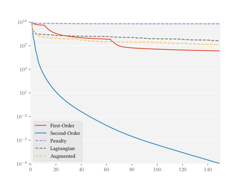
Figure 3. The figure compares convergent rate of first-order and second-order manifold optimization with the penalty, Lagrangian multiplier, and augmented Lagrangian methods. The results indicate the proposed first-order manifold optimization and second-order manifold optimization have faster convergence rates than the other methods.

Penalty Method

The penalty method uses an external potential to convert a constrained optimization problem to an unconstrained optimization problem, as shown in Equation 65.

(65) $$\operatorname*{arg\,min}_{\bm{x}}\Phi(\bm{x})+\frac{1}{2}\kappa\|C(\bm{x})\|^{2}$$

This method is commonly used in constrained optimization due to its simplicity. However, its shortcoming is that indefinite stiffness is required to satisfy constraints, and the introduced external stiffness $\kappa$ can make the entire system an ill-defined problem. In our experiments, we found that the penalty method failed to converge or converged very slowly when applied to quaternion-based optimization.

Lagrangian Multiplier

The Lagrangian multiplier adds external variables $\lambda$ to the system to change the constrained optimization problem to an unconstrained optimization problem, as shown in Equation 66.

(66) $$\operatorname*{arg\,min}_{\bm{x},\lambda}\Phi(\bm{x})+\lambda^{T}C(x)$$

One drawback of this method is the increase in the number of variables and computational cost. The actual degrees of freedom (DoFs) of rotation is 3, but the use of quaternions has already increased the number of unknowns to 4, and the addition of multipliers makes the number of variables 5. As the number of unknowns increases, the computational cost also increases. Additionally, we found that the convergence rate was even slower than that of our first-order manifold optimizer.

Augmented Lagrangian

The augmented Lagrangian method can be seen as a mix of the penalty method and the Lagrangian multiplier method, and turns constrained optimization problems into unconstrained optimization problems.

(67) $$\operatorname*{arg\,min}_{\bm{x},\lambda}\Phi(\bm{x})+\lambda^{T}C(x)+\frac{1}{2}\kappa\|C(\bm{x})\|^{2}$$

The external stiffness does not need to be infinite for the augmented Lagrangian method. However, in our experiments, the convergence rate was still lower than that of the manifold optimization method.

In conclusion, our proposed approach outperformed commonly used constrained optimization methods in terms of both convergence rate and performance.

8.2. Beam Stretch & Twist

In our experiment, we compared the simulation results of our implicit method with the explicit method proposed by (Lu et al., 2021). Specifically, we evaluated their performance in beam stretching and twisting scenarios, and found that both methods produced identical results under the same parameter settings.

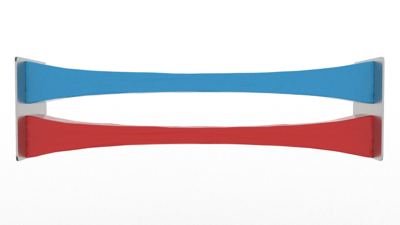
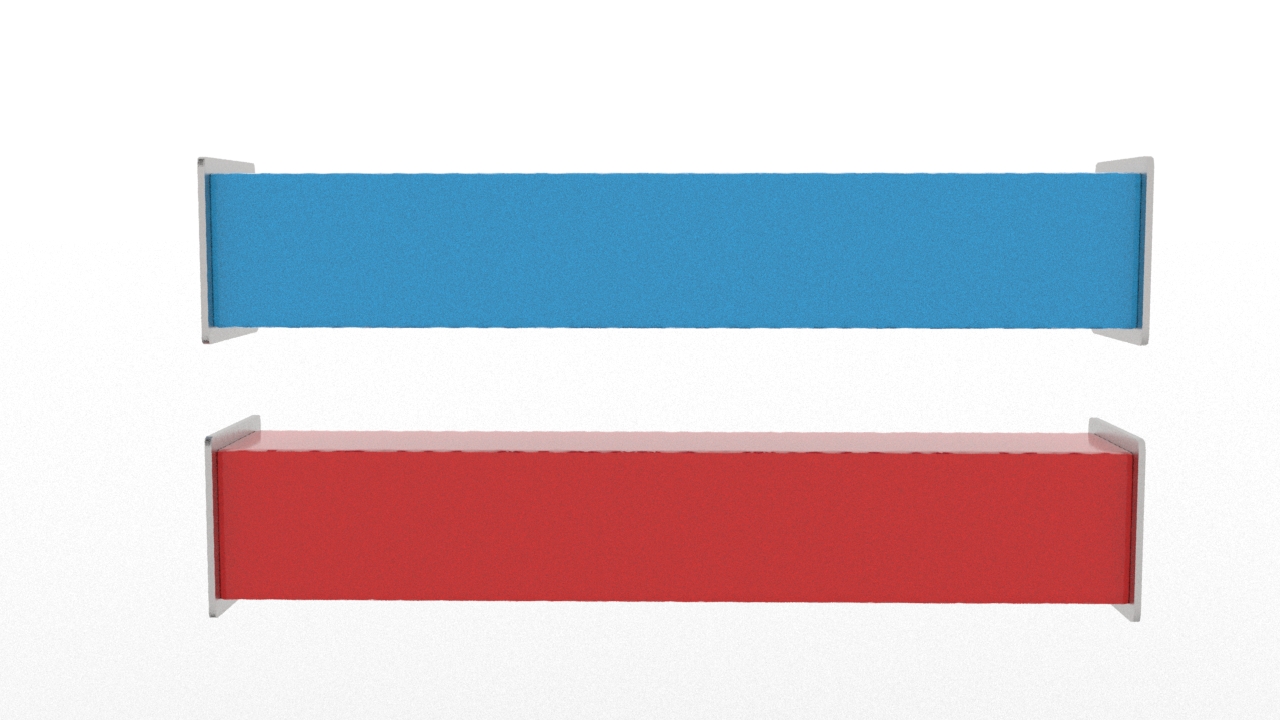
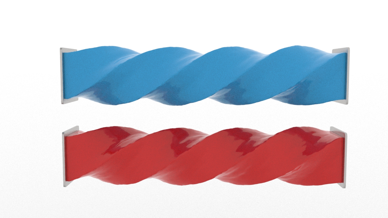
Figure 4. The figure compares explicit and implicit methods for simulating a stretched and twisted beam, finding that they can generate similar results.

8.3. Beam Drape

This experiment aims to investigate and compare the simulation time of the implicit and explicit simulation methods for varying stiffness levels and scales using the beam drape scenario. We plotted two curves to examine the relationship between simulation time and stiffness, as well as simulation time and scale. Our results show that the implicit method outperforms the explicit method by 3 to 6 times in terms of runtime.

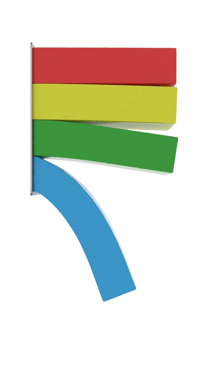
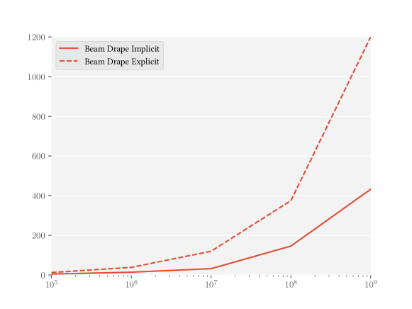
Figure 5. This experiment compares explicit and implicit methods for simulating beam drape. The curve showcases the relationship between computational cost and material stiffness, demonstrating that implicit methods produce faster results for a range of stiffness values.

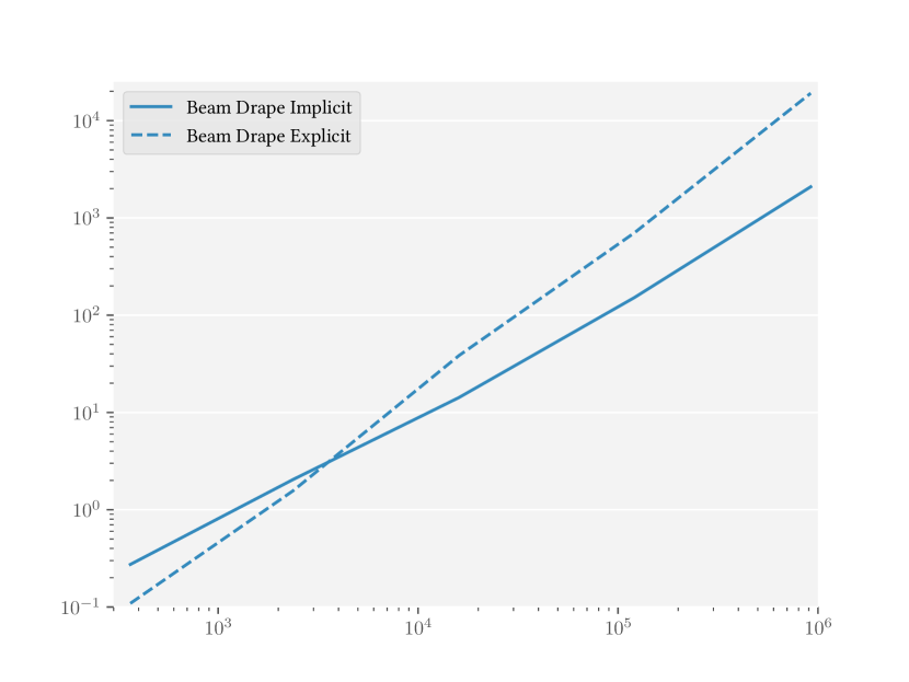
Figure 6. This experiment compares explicit and implicit methods for simulating beam drape, showcasing the relationship between computational cost and simulated discrete elements. Findings demonstrate that implicit methods significantly outperform explicit methods for finer simulation scales.

8.4. Chocolate

For this experiment, we simulated a chocolate drop with a middle stiffness to compare the time cost in contact-rich scenes between the implicit and explicit simulation methods. Our results show that the implicit method had a 3 times speedup compared to the explicit method. The visualization of the simulation result can be found in figure 2.

8.5. Plate

In this experiment, we compare the computational efficiency of the implicit and explicit methods with high stiffness for simulating the fracture of a plate during a drop to the ground. We found that our method provided a four-fold increase in speed compared to the explicit method under these conditions. The results of our simulation are presented in figure 1.

9. Conclusion

In conclusion, our paper investigates a variational integrator for implicit solving of quaternion-based systems. We also showcase the efficacy of manifold optimization techniques for quaternion constraints, which are faster than commonly used techniques like penalty methods, Lagrangian multipliers, and augmented Lagrangian method. We also introduced the nullspace operator in manifold optimization, which simplifies the optimization problem and reduces the number of unknowns. Our variational integrator and manifold technique can be used in other quaternion-based system simulations.

Furthermore, we proposed a new implicit method for simulating bonded discrete element systems utilizing our variational integrator and manifold optimization approach. We utilized the semi-positive definite projection method with preconditioned conjugate gradient and line search method on the manifold, and subsequently proposed a stable integrator. Our results demonstrate that our method can achieve the same simulation results as the explicit method while providing faster computation times. Additionally, we have shown that our method can accept large steps for simulation while still ensuring high accuracy.

Moreover, we have introduced a new method for packing and reconstruction of fracture surfaces for visualization. This method is suitable for bonded discrete element method and can provide accurate fracture surface in complicated fracture scenarios in a simple and fast manner.

As we have showcased the potential of our variational integrator and manifold optimization approach in this paper, our future work includes expanding our research scope to address promising avenues for improvement. This will involve implementing a GPU version of our algorithm to extend the scale of our simulations to larger systems, as well as coupling finite element method with discrete element method to further enhance the accuracy and efficiency of our simulations.

References

- (1)
- Alduán et al. (2009) Iván Alduán, Angel Tena, and Miguel A Otaduy. 2009. Simulation of High-Resolution Granular Media.. In CEIG. 11–18.
- André et al. (2012) Damien André, Ivan Iordanoff, Jean-luc Charles, and Jérôme Néauport. 2012. Discrete element method to simulate continuous material by using the cohesive beam model. Computer methods in applied mechanics and engineering 213 (2012), 113–125.
- Bao et al. (2007) Zhaosheng Bao, Jeong-Mo Hong, Joseph Teran, and Ronald Fedkiw. 2007. Fracturing rigid materials. IEEE Transactions on Visualization and Computer Graphics 13, 2 (2007), 370–378.
- Baraff and Witkin (1998) David Baraff and Andrew Witkin. 1998. Large steps in cloth simulation. In Proceedings of ACM SIGGRAPH 1998. 43–54.
- Batty et al. (2012) Christopher Batty, Andres Uribe, Basile Audoly, and Eitan Grinspun. 2012. Discrete viscous sheets. ACM Transactions on Graphics (TOG) 31, 4 (2012), 1–7.
- Bell et al. (2005) Nathan Bell, Yizhou Yu, and Peter J Mucha. 2005. Particle-based simulation of granular materials. In Proceedings of the 2005 ACM SIGGRAPH/Eurographics symposium on Computer animation. 77–86.
- Bergou et al. (2008) Miklós Bergou, Max Wardetzky, Stephen Robinson, Basile Audoly, and Eitan Grinspun. 2008. Discrete elastic rods. In ACM SIGGRAPH 2008 papers. 1–12.
- Betsch and Siebert (2009) Peter Betsch and Ralf Siebert. 2009. Rigid body dynamics in terms of quaternions: Hamiltonian formulation and conserving numerical integration. International journal for numerical methods in engineering 79, 4 (2009), 444–473.
- Boumal (2022) Nicolas Boumal. 2022. An introduction to optimization on smooth manifolds. To appear with Cambridge University Press. https://www.nicolasboumal.net/book
- Chen et al. (2018) Wei Chen, Fei Zhu, Jing Zhao, Sheng Li, and Guoping Wang. 2018. Peridynamics-Based Fracture Animation for Elastoplastic Solids. In Computer Graphics Forum, Vol. 37. Wiley Online Library, 112–124.
- Chen et al. (2017) Yu Ju Chen, Uri M Ascher, and Dinesh K Pai. 2017. Exponential rosenbrock-euler integrators for elastodynamic simulation. IEEE Transactions on Visualization and Computer Graphics 24, 10 (2017), 2702–2713.
- Chen et al. (2014) Zhili Chen, Miaojun Yao, Renguo Feng, and Huamin Wang. 2014. Physics-inspired adaptive fracture refinement. ACM Transactions on Graphics (TOG) 33, 4 (2014), 1–7.
- Chitalu et al. (2020) Floyd M Chitalu, Qinghai Miao, Kartic Subr, and Taku Komura. 2020. Displacement-Correlated XFEM for Simulating Brittle Fracture. In Computer Graphics Forum, Vol. 39. Wiley Online Library, 569–583.
- Cundall (1971) P. A. Cundall. 1971. A Computer Model for Simulating Progressive, Large-scale Movement in Blocky Rock System. Proceedings of the International Symposium on Rock Mechanics (1971).
- Cundall and Strack (1979) P. A. Cundall and O. D. L. Strack. 1979. A discrete numerical model for granular assemblies. Géotechnique 29, 1 (1979), 47–65.
- De Klerk et al. (2022) David N De Klerk, Thomas Shire, Zhiwei Gao, Andrew T McBride, Christopher J Pearce, and Paul Steinmann. 2022. A variational integrator for the Discrete Element Method. J. Comput. Phys. 462 (2022), 111253.
- Dinev et al. (2018) Dimitar Dinev, Tiantian Liu, and Ladislav Kavan. 2018. Stabilizing integrators for real-time physics. ACM Transactions on Graphics (TOG) 37, 1 (2018), 1–19.
- Eberhardt et al. (2000) Bernhard Eberhardt, Olaf Etzmuß, and Michael Hauth. 2000. Implicit-explicit schemes for fast animation with particle systems. In Computer Animation and Simulation 2000: Proceedings of the Eurographics Workshop in Interlaken, Switzerland, August 21–22, 2000. Springer, 137–151.
- Gast et al. (2015) Theodore F Gast, Craig Schroeder, Alexey Stomakhin, Chenfanfu Jiang, and Joseph M Teran. 2015. Optimization integrator for large time steps. IEEE transactions on visualization and computer graphics 21, 10 (2015), 1103–1115.
- Hahn and Wojtan (2015) David Hahn and Chris Wojtan. 2015. High-resolution brittle fracture simulation with boundary elements. ACM Transactions on Graphics (TOG) 34, 4 (2015), 1–12.
- Hahn and Wojtan (2016) David Hahn and Chris Wojtan. 2016. Fast approximations for boundary element based brittle fracture simulation. ACM Transactions on Graphics (TOG) 35, 4 (2016), 1–11.
- Harmon et al. (2009) David Harmon, Etienne Vouga, Breannan Smith, Rasmus Tamstorf, and Eitan Grinspun. 2009. Asynchronous contact mechanics. In ACM SIGGRAPH 2009 papers. 1–12.
- Hellrung et al. (2009) Jeffrey Hellrung, Andrew Selle, Arthur Shek, Eftychios Sifakis, and Joseph Teran. 2009. Geometric fracture modeling in Bolt. In SIGGRAPH 2009: Talks. 1–1.
- Hirota et al. (2001) Gentaro Hirota, Susan Fisher, A State, Chris Lee, and Henry Fuchs. 2001. An implicit finite element method for elastic solids in contact. In Proceedings Computer Animation 2001. Fourteenth Conference on Computer Animation (Cat. No. 01TH8596). IEEE, 136–254.
- Johnson et al. (2014) Elliot Johnson, Jarvis Schultz, and Todd Murphey. 2014. Structured linearization of discrete mechanical systems for analysis and optimal control. IEEE Transactions on Automation Science and Engineering 12, 1 (2014), 140–152.
- Joshuah et al. (2020) Wolper Joshuah, Chen Yunuo, Li Minchen, Fang Yu, Qu Ziyin, Lu Jiecong, Cheng Meggie, and Jiang Chenfanfu. 2020. Anisompm: Animating anisotropic damage mechanics. ACM Transactions on Graphics (TOG) 39, 4 (2020), 37–1.
- Kane et al. (2000) Couro Kane, Jerrold E Marsden, Michael Ortiz, and Matthew West. 2000. Variational integrators and the Newmark algorithm for conservative and dissipative mechanical systems. International Journal for numerical methods in engineering 49, 10 (2000), 1295–1325.
- Karamouzas et al. (2017) Ioannis Karamouzas, Nick Sohre, Rahul Narain, and Stephen J Guy. 2017. Implicit crowds: Optimization integrator for robust crowd simulation. ACM Transactions on Graphics (TOG) 36, 4 (2017), 1–13.
- Kaufmann et al. (2009) Peter Kaufmann, Sebastian Martin, Mario Botsch, Eitan Grinspun, and Markus Gross. 2009. Enrichment textures for detailed cutting of shells. In ACM SIGGRAPH 2009 papers. 1–10.
- Kee et al. (2023) Min Hyung Kee, Kiwon Um, HyunMo Kang, and JungHyun Han. 2023. An Optimization-based SPH Solver for Simulation of Hyperelastic Solids. In Computer Graphics Forum, Vol. 42. Wiley Online Library, 225–233.
- Kharevych et al. (2006) Liliya Kharevych, W Wei, Yiying Tong, Eva Kanso, Jerrold E Marsden, Peter Schröder, and Matthieu Desbrun. 2006. Geometric, variational integrators for computer animation. Eurographics Association.
- Koschier et al. (2017) Dan Koschier, Jan Bender, and Nils Thuerey. 2017. Robust eXtended finite elements for complex cutting of deformables. ACM Transactions on Graphics (TOG) 36, 4 (2017), 1–13.
- Koschier et al. (2014) Dan Koschier, Sebastian Lipponer, and Jan Bender. 2014. Adaptive Tetrahedral Meshes for Brittle Fracture Simulation.. In Symposium on Computer Animation, Vol. 3.
- Kugelstadt and Schömer (2016) Tassilo Kugelstadt and Elmar Schömer. 2016. Position and orientation based Cosserat rods.. In Symposium on Computer Animation. 169–178.
- Lew and Mata A (2016) Adrián J Lew and Pablo Mata A. 2016. A brief introduction to variational integrators. Structure-preserving integrators in nonlinear structural dynamics and flexible multibody dynamics (2016), 201–291.
- Li et al. (2020) Minchen Li, Zachary Ferguson, Teseo Schneider, Timothy R Langlois, Denis Zorin, Daniele Panozzo, Chenfanfu Jiang, and Danny M Kaufman. 2020. Incremental potential contact: intersection-and inversion-free, large-deformation dynamics. ACM Trans. Graph. 39, 4 (2020), 49.
- Li et al. (2019) Minchen Li, Ming Gao, Timothy Langlois, Chenfanfu Jiang, and Danny M Kaufman. 2019. Decomposed optimization time integrator for large-step elastodynamics. ACM Transactions on Graphics (TOG) 38, 4 (2019), 1–10.
- Liu et al. (2013) Tiantian Liu, Adam W Bargteil, James F O’Brien, and Ladislav Kavan. 2013. Fast simulation of mass-spring systems. ACM Transactions on Graphics (TOG) 32, 6 (2013), 1–7.
- Löschner et al. (2020) Fabian Löschner, Andreas Longva, Stefan Jeske, Tassilo Kugelstadt, and Jan Bender. 2020. Higher-order time integration for deformable solids. In Computer Graphics Forum, Vol. 39. Wiley Online Library, 157–169.
- Lu et al. (2021) Jia-Ming Lu, Chen-Feng Li, Geng-Chen Cao, and Shi-Min Hu. 2021. Simulating Fractures With Bonded Discrete Element Method. IEEE Transactions on Visualization and Computer Graphics 28, 12 (2021), 4810–4824.
- Martin et al. (2011) Sebastian Martin, Bernhard Thomaszewski, Eitan Grinspun, and Markus Gross. 2011. Example-based elastic materials. In ACM SIGGRAPH 2011 papers. 1–8.
- Michels et al. (2014) Dominik L Michels, Gerrit A Sobottka, and Andreas G Weber. 2014. Exponential integrators for stiff elastodynamic problems. ACM Transactions on Graphics (TOG) 33, 1 (2014), 1–20.
- Molino et al. (2004) Neil Molino, Zhaosheng Bao, and Ron Fedkiw. 2004. A virtual node algorithm for changing mesh topology during simulation. ACM Transactions on Graphics (TOG) 23, 3 (2004), 385–392.
- Müller and Chentanez (2011) Matthias Müller and Nuttapong Chentanez. 2011. Solid simulation with oriented particles. In ACM SIGGRAPH 2011 papers. 1–10.
- Müller et al. (2013) Matthias Müller, Nuttapong Chentanez, and Tae-Yong Kim. 2013. Real time dynamic fracture with volumetric approximate convex decompositions. ACM Transactions on Graphics (TOG) 32, 4 (2013), 1–10.
- Müller et al. (2001) Matthias Müller, Leonard McMillan, Julie Dorsey, and Robert Jagnow. 2001. Real-time simulation of deformation and fracture of stiff materials. In Computer Animation and Simulation 2001. 113–124.
- Nesme et al. (2009) Matthieu Nesme, Paul G Kry, Lenka Jeřábková, and François Faure. 2009. Preserving topology and elasticity for embedded deformable models. In ACM SIGGRAPH 2009 papers. 1–9.
- Nguyen et al. (2021) Vinh DX Nguyen, A Kiet Tieu, Damien André, Lihong Su, and Hongtao Zhu. 2021. Discrete element method using cohesive plastic beam for modeling elasto-plastic deformation of ductile materials. Computational Particle Mechanics 8 (2021), 437–457.
- O’Brien and Hodgins (1999) James F. O’Brien and Jessica K. Hodgins. 1999. Graphical Modeling and Animation of Brittle Fracture. In Proceedings of ACM SIGGRAPH 1999. 137–146.
- Pauly et al. (2005) Mark Pauly, Richard Keiser, Bart Adams, Philip Dutré, Markus Gross, and Leonidas J Guibas. 2005. Meshless animation of fracturing solids. ACM Transactions on Graphics (TOG) 24, 3 (2005), 957–964.
- Pfaff et al. (2014) Tobias Pfaff, Rahul Narain, Juan Miguel De Joya, and James F O’Brien. 2014. Adaptive tearing and cracking of thin sheets. ACM Transactions on Graphics (TOG) 33, 4 (2014), 1–9.
- Potyondy and Cundall (2004) David O Potyondy and PA Cundall. 2004. A bonded-particle model for rock. International journal of rock mechanics and mining sciences 41, 8 (2004), 1329–1364.
- Raghavachary (2002) Saty Raghavachary. 2002. Fracture generation on polygonal meshes using Voronoi polygons. In ACM SIGGRAPH 2002 conference abstracts and applications. 187–187.
- Rungjiratananon et al. (2008) Witawat Rungjiratananon, Zoltan Szego, Yoshihiro Kanamori, and Tomoyuki Nishita. 2008. Real-time animation of sand-water interaction. In Computer Graphics Forum, Vol. 27. 1887–1893.
- Saemundsson et al. (2020) Steindor Saemundsson, Alexander Terenin, Katja Hofmann, and Marc Deisenroth. 2020. Variational integrator networks for physically structured embeddings. In International Conference on Artificial Intelligence and Statistics. PMLR, 3078–3087.
- Schvartzman and Otaduy (2014) Sara C Schvartzman and Miguel A Otaduy. 2014. Fracture animation based on high-dimensional voronoi diagrams. In Proceedings of the 18th Meeting of the ACM SIGGRAPH Symposium on Interactive 3D Graphics and Games. 15–22.
- Sifakis et al. (2007) Eftychios Sifakis, Kevin G Der, and Ronald Fedkiw. 2007. Arbitrary cutting of deformable tetrahedralized objects. In Proceedings of the 2007 ACM SIGGRAPH/Eurographics symposium on Computer animation. 73–80.
- Soler et al. (2018) Carlota Soler, Tobias Martin, and Olga Sorkine-Hornung. 2018. Cosserat rods with projective dynamics. In Computer Graphics Forum, Vol. 37. 137–147.
- Stern and Grinspun (2009) Ari Stern and Eitan Grinspun. 2009. Implicit-explicit variational integration of highly oscillatory problems. Multiscale Modeling & Simulation 7, 4 (2009), 1779–1794.
- Su et al. (2009) Jonathan Su, Craig Schroeder, and Ronald Fedkiw. 2009. Energy stability and fracture for frame rate rigid body simulations. In Proceedings of the 2009 ACM SIGGRAPH/Eurographics Symposium on Computer Animation. 155–164.
- Thomaszewski et al. (2008) Bernhard Thomaszewski, Simon Pabst, and Wolfgang Straßer. 2008. Asynchronous cloth simulation. In Computer Graphics International, Vol. 2. Citeseer, 2.
- Trusty et al. (2022) Ty Trusty, Danny Kaufman, and David IW Levin. 2022. Mixed variational finite elements for implicit simulation of deformables. In SIGGRAPH Asia 2022 Conference Papers. 1–8.
- Volino and Magnenat-Thalmann (2001) Pascal Volino and Nadia Magnenat-Thalmann. 2001. Comparing efficiency of integration methods for cloth simulation. In Proceedings. Computer Graphics International 2001. IEEE, 265–272.
- Wang et al. (2020) Xinlei Wang, Minchen Li, Yu Fang, Xinxin Zhang, Ming Gao, Min Tang, Danny M Kaufman, and Chenfanfu Jiang. 2020. Hierarchical optimization time integration for cfl-rate mpm stepping. ACM Transactions on Graphics (TOG) 39, 3 (2020), 1–16.
- Wicke et al. (2010) Martin Wicke, Daniel Ritchie, Bryan M Klingner, Sebastian Burke, Jonathan R Shewchuk, and James F O’Brien. 2010. Dynamic local remeshing for elastoplastic simulation. ACM Transactions on graphics (TOG) 29, 4 (2010), 1–11.
- Wojtan and Turk (2008) Chris Wojtan and Greg Turk. 2008. Fast viscoelastic behavior with thin features. In ACM SIGGRAPH 2008 papers. 1–8.
- Wolper et al. (2019) Joshuah Wolper, Yu Fang, Minchen Li, Jiecong Lu, Ming Gao, and Chenfanfu Jiang. 2019. CD-MPM: continuum damage material point methods for dynamic fracture animation. ACM Transactions on Graphics (TOG) 38, 4 (2019), 1–15.
- Yue et al. (2018) Yonghao Yue, Breannan Smith, Peter Yichen Chen, Maytee Chantharayukhonthorn, Ken Kamrin, and Eitan Grinspun. 2018. Hybrid grains: adaptive coupling of discrete and continuum simulations of granular media. ACM Transactions on Graphics (TOG) 37, 6 (2018), 1–19.
- Zheng and James (2010) Changxi Zheng and Doug L James. 2010. Rigid-body fracture sound with precomputed soundbanks. In ACM SIGGRAPH 2010 papers. 1–13.
- Zhu et al. (2015) Yufeng Zhu, Robert Bridson, and Chen Greif. 2015. Simulating rigid body fracture with surface meshes. ACM Transactions on Graphics (TOG) 34, 4 (2015), 1–11.