The stochastic fractional Strichartz estimate and blow-up for Schrödinger equation

Abstract

We establish the stochastic Strichartz estimate for the fractional Schrödinger equation with multiplicative noise. With the help of the deterministic Strichartz estimates, we prove the existence and uniqueness of a global solution to the stochastic fractional nonlinear Schrödinger equation in $L^{2}(\mathbb{R}^{n})$. In addition, we give a general blow-up result by deriving a localized virial estimate and the generalized Strauss inequality with a restricted class of initial data.

1 Introduction.

The fractional nonlinear Schrödinger equation appears in various fields such as nonlinear optics [1], quantum physics [2] and water propagation [3]. Inspired by the Feynman path approach to quantum mechanics, Laskin [4] used the path integral over Lévy-like quantum mechanical paths to obtain a fractional Schrödinger equation. Kirkpatrick et.al. [5] considered a general class of discrete nonlinear Schrödinger equations on the lattice $h\mathbb{Z}$ with mesh size $h>0$, they showed that the limiting dynamics were given by a nonlinear fractional Schrödinger equation when $h\rightarrow 0$. Guo and Huang [6] applied concentration compactness and commutator estimates to obtain the existence of standing waves for nonlinear fractional Schrödinger equations under some assumptions. Shang and Zhang [7] studied the existence and multiplicity of solutions for the critical fractional Schrödinger equation. They proved that the equation had a nonnegative ground state solution and also investigated the relation between the number of solutions and the topology of the set. Choi and Aceves [8] proved that the solutions of the discrete nonlinear Schrödinger equation with non-local algebraically decaying coupling converged strongly in $L^{2}(\mathbb{R}^{n})$ to those of the continuum fractional nonlinear Schrödinger equation. Frank and his collaborators [9] proved general uniqueness results for radial solutions of linear and nonlinear equations involving the fractional Laplacian $(-\Delta)^{\alpha}$ with $\alpha\in(0,1)$ for any space dimensions $N\geq 1$. Wang and Huang [10] proposed an energy conservative difference scheme for the nonlinear fractional Schrödinger equations and gave a rigorous analysis of the conservation property.

In some circumstances, randomness has to be taken into account. The understanding of the influence of noise on the propagation of waves is a very important problem. It can change drastically the qualitative behaviors and results in new properties. For the stochastic Schödinger equation driven by Gaussian noise, Bouard and Debussche [11, 12] studied a conservative stochastic nonlinear Schrödinger equation and the influence of multiplicative Gaussian noise, and showed the global existence and uniqueness of solutions. Herr et.al. [13] studied the scattering behavior of global solutions for the stochastic nonlinear Schrödinger equations with linear multiplicative noise. Barbu and his collaborators [14] showed the explosion even could be prevented with high probability on the whole time interval $[0,\infty)$. Debussche and Menza [15] numerically investigated nonlinear Schrödinger equations with a stochastic contribution. Brzeźniak et.al. [16] established a new version of the stochastic Strichartz estimate for the stochastic convolution driven by jump noise. Deng et.al. [17] studied the propagation of randomness under nonlinear dispersive equations by the theory of random tensors. Cui et.al. [18] demonstrated that the solutions of stochastic nonlinear Schrödinger equations can be approximated by the solutions of coupled splitting systems. Yuan and Chen [19] proved the existence of martingale solutions for the stochastic fractional nonlinear Schrödinger equation on a bounded interval.

There has been a lot of interest in the study of blow-up for fractional Schrödinger equation. Dinh [20] studied dynamical properties of blow-up solutions to the focusing mass-critical nonlinear fractional Schrödinger equation, and obtained the $L^{2}$-concentration and the limiting profile with minimal mass of blow-up solutions. Boulenger et.al. [21] derived a localized virial estimate for fractional nonlinear Schrödinger equation in $\mathbb{R}^{n}$ and proved the general blow-up result. Zhu and his collaborators [22, 23] found the sharp threshold mass of the existence of finite-time blow-up solutions and the sharp threshold of the scattering versus blow-up dichotomy for radial data. Barbu et.al. [24] devoted to the study of noise effects on blow-up solutions to stochastic nonlinear Schrödinger equations. Lan [25] showed that if the initial data had negative energy and slightly supercritical mass, the solution for $L^{2}$-critical fractional Schrödinger equations blew up in finite time.

In this paper, we examine the following stochastic fractional nonlinear Schrödinger equation with multiplicative noise in $L^{2}(\mathbb{R}^{n})$,

$$\left\{\begin{aligned} &idu-\left[(-\Delta)^{\alpha}u-|u|^{2\sigma}u\right]dt=u\circ dW(t),\quad x\in\mathbb{R}^{n},\quad t\geq 0,\\ &u(0)=u_{0},\end{aligned}\right.$$ (1.1)

where $u$ is a complex valued process defined on $\mathbb{R}^{n}\times\mathbb{R}^{+}$, $0<\sigma<\infty$, and $W(t)$ is a $Q$-Wiener process. The fractional Laplacian operator $(-\Delta)^{\alpha}$ with admissible exponent $\alpha\in(0,1)$ is involved. The notation $\circ$ stands for Stratonovitch integral.

Let $(\Omega,\mathcal{F},\mathbb{P})$ be a probability space, $\left(\mathcal{F}_{t}\right)_{t\geq 0}$ be a filtration, and let $\left(\beta_{k}\right)_{k\in\mathbb{N}}$ be a sequence of independent Brownian motions associated to this filtration. Given $\left(e_{k}\right)_{k\in\mathbb{N}}$ an orthonormal basis of $L^{2}\left(\mathbb{R}^{n},\mathbb{R}\right)$, and a linear operator $\Phi$ on $L^{2}\left(\mathbb{R}^{n},\mathbb{R}\right)$ with a real-valued kernel $k$:

$$\Phi h(x)=\int_{\mathbb{R}^{n}}k(x,y)h(y)dy,\quad h\in L^{2}\left(\mathbb{R}^{n},\mathbb{R}\right).$$ (1.2)

Then the process

$$W(t,x,\omega):=\sum_{k=0}^{\infty}\beta_{k}(t,\omega)\Phi e_{k}(x),\quad t\geq 0,\quad x\in\mathbb{R}^{n},\quad\omega\in\Omega$$

is a Wiener process on $L^{2}\left(\mathbb{R}^{n},\mathbb{R}\right)$ with covariance operator $\Phi\Phi^{*}$, and the equation (1.1) can be rewritten as

$$idu-\left[(-\Delta)^{\alpha}u-|u|^{2\sigma}u\right]dt=udW-\frac{1}{2}iuF_{\Phi}dt,$$ (1.3)

where the function $F_{\Phi}$ is given by

$$F_{\Phi}(x)=\sum_{k=0}^{\infty}\left(\Phi e_{k}(x)\right)^{2},\quad x\in\mathbb{R}^{n}.$$ (1.4)

In the framework of stochastic mechanics, there are few results on the existence and uniqueness of a global solution for the stochastic fractional nonlinear Schrödinger equation in $L^{2}(\mathbb{R}^{n})$, and the general critical for blowing up of solutions, due to the complexity brought by the fractional Laplacian operator and white noise. Here we are particularly interested in the influence of noise acting as a potential on this behavior. In contrast to the case of stochastic nonlinear Schrödinger equation in $L^{2}(\mathbb{R}^{n})$. There are some essential difficulties in our problems. The first difficulty is the appearance of the fractional Laplacian operator $(-\Delta)^{\alpha}$. The deterministic cubic fractional nonlinear Schrödinger equation is ill-posedness in $L^{2}(\mathbb{R}^{n})$ (see e.g., Ref. [26]). The natural question now is whether one can get quantitative information on the stochastic fractional nonlinear Schrödinger equation in $L^{2}(\mathbb{R}^{n})$. The second difficulty lies in the fact that the classical virial theorem may not be applicable anymore. When $\alpha=1$, one can compute easily the time derivative of the virial action. In the case $\alpha\in(\frac{1}{2},1)$, it’s quite difficult to obtain the time derivative of the virial action. So we need some new techniques to derive a stochastic version variance identity, which is a crucial tool to prove the occurrence of a blow-up for a restricted class of initial data.

This paper is organized as follows. In Section 2, we introduce some notations and state our main results in this present paper. In Section 3, we construct a truncated equation and prove the existence of a local solution of equation (1.1) in the whole space. Meanwhile, we use the stopping time technique, deterministic and stochastic fractional Strichartz inequalities to prove the global existence of the original equation (1.1). In Section 4, we establish a sufficient criterion for blow-up of radial solution. In section 5, we give a specific example to understand the influence of noise on the propagation of waves. Some tedious proofs of lemmas are left in Appendix A.

2 Notations and main results

We introduce some notations throughout this paper. The capital letter $C$ denotes a positive constant, whose value may change from one line to another. The notation $C_{p}$ is used to emphasize that the constant only depends on the parameter $p$, while $C(\cdot\cdot\cdot)$ is used for the case that there are more than one parameter. For $p\geq 2$, the notation $L^{p}$ denotes the Lebesgue space of complex-valued functions. The inner product in $L^{2}\left(\mathbb{R}^{n}\right)$ is endowed with

$$(f,g)={\bf{Re}}\int_{\mathbb{R}^{n}}f(x)\bar{g}(x)dx,$$ (2.1)

for $f,g\in L^{2}\left(\mathbb{R}^{n}\right)$.

Given a Banach space $B$, we denote by $R(H;B)$ the $\gamma$-radonifying operator from $H$ into $B$ (see e.g., Ref. [27]), equipped with the norm

$$\|K\|^{2}_{R(H,B)}=\widetilde{\mathbb{E}}\left|\sum_{k=1}^{\infty}\gamma_{k}Ke_{k}\right|^{2}_{B},$$ (2.2)

where $(e_{k})_{k\in\mathbb{N}}$ is any orthonormal basis of $H$, and $(\gamma_{k})_{k\in\mathbb{N}}$ is any sequence of independent normal real-valued random variables on a probability space $\left(\widetilde{\Omega},\widetilde{\mathcal{F}},\widetilde{P}\right)$. The notation $\widetilde{E}$ denotes the expectation on $\left(\widetilde{\Omega},\widetilde{\mathcal{F}},\widetilde{P}\right)$.

Given two separable Hilbert spaces $H$ and $\widetilde{H}$, the notation $L^{0}_{2}\left(H;\widetilde{H}\right)$ denotes the space of Hilbert-Schmidt operators from $H$ into $\widetilde{H}$. When $H=\widetilde{H}=L^{2}(\mathbb{R}^{n};\mathbb{R})$, $L^{0}_{2}\left(L^{2}(\mathbb{R}^{n};\mathbb{R}),L^{2}(\mathbb{R}^{n};\mathbb{R})\right)$ is simply denoted by $L^{0}_{2}$. We also use $\nabla$ to denote the gradient operator in Euclidean space. Let $\Phi:H\rightarrow\widetilde{H}$ be a bounded linear operator. The operator $\Phi$ is called the Hilbert-Schmidt operator if there is an orthonormal basis $(e_{k})_{k\in\mathbb{N}}$ in $H$ such that

$$\|\Phi\|^{2}_{L^{0}_{2}(H;\widetilde{H})}=\operatorname{tr}\Phi^{*}\Phi=\sum_{k\in\mathbb{N}}\left|\Phi e_{k}\right|_{\widetilde{H}}^{2}<\infty.$$ (2.3)

In the following, we review the concept of fractional derivatives. The fractional Laplace operator $(-\Delta)^{\alpha}$ with $\alpha\in(0,1)$ is given by

$$(-\Delta)^{\alpha}u(x)=C(n,\alpha)~{}\rm{P.V.}\int_{\mathbb{R}^{n}}\frac{u(x)-u(y)}{|x-y|^{n+2\alpha}}dy,\\$$

where $\rm{P.V.}$ means the principle value of the integral, and $C(n,\alpha)$ is a positive constant given by

$$C(n,\alpha)=\frac{\alpha 4^{\alpha}\Gamma(\frac{n+2\alpha}{2})}{\pi^{\frac{n}{2}}\Gamma(1-\alpha)}.$$ (2.4)

For every $\alpha\in(0,1)$, the space $H^{\alpha}(\mathbb{R}^{n})$ is denoted by

$$H^{\alpha}(\mathbb{R}^{n})=\left\{u\in L^{2}(\mathbb{R}^{n}):\int_{\mathbb{R}^{n}}\int_{\mathbb{R}^{n}}\frac{|u(x)-u(y)|^{2}}{|x-y|^{n+2\alpha}}dxdy<\infty\right\}.$$

Then $H^{\alpha}(\mathbb{R}^{n})$ is a Hilbert space with inner product given by

$$(u,v)_{H^{\alpha}(\mathbb{R}^{n})}=(u,v)_{L^{2}(\mathbb{R}^{n})}+\int_{\mathbb{R}^{n}}\int_{\mathbb{R}^{n}}\frac{|u(x)-u(y)|^{2}}{|x-y|^{n+2\alpha}}dxdy.$$

In the following, we also give the notation

$$(u,v)_{\dot{H}^{\alpha}(\mathbb{R}^{n})}=\int_{\mathbb{R}^{n}}\int_{\mathbb{R}^{n}}\frac{|u(x)-u(y)|^{2}}{|x-y|^{n+2\alpha}}dxdy.$$

Then we have

$$(u,v)_{H^{\alpha}(\mathbb{R}^{n})}=(u,v)_{L^{2}(\mathbb{R}^{n})}+(u,v)_{\dot{H}^{\alpha}(\mathbb{R}^{n})}.$$

By the result from the reference [28, Proposition 3.6], we know that

$$\|(-\Delta)^{\frac{\alpha}{2}}u\|^{2}_{L^{2}(\mathbb{R}^{n})}=\frac{1}{2}C(n,\alpha)\|u\|^{2}_{\dot{H}^{\alpha}(\mathbb{R}^{n})}.$$

Our first result is as follows.

Theorem 1.

Assume that $0<\sigma<\frac{2}{n}$ if  $n=1$ or  $2$; $0<\sigma<\frac{1}{n-1}$ if $n\geq 3$. Let $\Phi\in{L}_{2}^{0}\cap R\left(L^{2}({\mathbb{R}^{n};\mathbb{R}}),L^{2+\delta}\left(\mathbb{R}^{n}\right)\right)$ for some $\delta>2(n-1)$. Let $\alpha\in\left[\frac{n}{2n-1},1\right)$, $p\geq\max\left(2\sigma+2,\frac{2(2+\delta)}{\delta}\right)$ with the additional assumption that $p<\frac{2n}{n-\alpha}$ if $n\geq 2$, and let $r$ be such that $\frac{2}{r}=$ $\frac{n}{\alpha}\left(\frac{1}{2}-\frac{1}{p}\right)$. Furthermore, we suppose that the initial value $u_{0}$ is radial; then for any $\rho\geq\max\left(r,(2\sigma+2)\left(\frac{4\sigma}{2-n\sigma}+1\right)\right)$, $u_{0}\in L^{\rho}\left(\Omega;L^{2}\left(\mathbb{R}^{n}\right)\right)$ with $\mathcal{F}_{0}$-measurable and $T_{0}>0$, there is a unique radial solution $u$ of (1.1), such that $u\in L^{\rho}\left(\Omega;\mathcal{C}\left(\left[0,T_{0}\right];L^{2}\left(\mathbb{R}^{n}\right)\right)\right)\cap L^{1}\left(\Omega;L^{r}\left(0,T_{0};L^{p}\left(\mathbb{R}^{n}\right)\right)\right)$. Moreover, for a.e. $\omega\in\Omega$, and each $t\in\left[0,T_{0}\right]$, we have

$$|u(t)|_{L^{2}\left(\mathbb{R}^{n}\right)}=\left|u_{0}\right|_{L^{2}\left(\mathbb{R}^{n}\right)}.$$ (2.5)

Our second main result establishes a sufficient criterion for the blow-up of radial solutions.

Theorem 2.

Assume that the initial value $u_{0}$ is radial and $u\in C([0,T);H^{2\alpha}(\mathbb{R}^{n}))$ is a radial solution of stochastic fractional nonlinear Schrödinger equation (1.1). Let $n\geq 2$, $\alpha\in\left[\frac{n}{2n-1},1\right),\frac{2\alpha}{n}\leq\sigma\leq\frac{2\alpha}{n-2\alpha}$ with $\sigma<2\alpha$. Furthermore, we suppose that there exists a positive constant $\widetilde{\mathcal{R}}$, such that

$$\sum_{k=0}^{\infty}\int_{\mathbb{R}^{n}}\frac{\left(\Phi e_{k}(x)-\Phi e_{k}(y)\right)^{2}}{|x-y|^{n+2\alpha}}dy\leq{\mathcal{R}},$$ (2.6)

and for some $t>0$,

$$\mathbb{E}[H(u_{0})]+\frac{1}{4}tC_{n,\alpha}{\mathcal{R}}\mathbb{E}[M(u_{0})]<0.$$ (2.7)

Then $u(t)$ blows up in finite time in the sense that $T<+\infty$.

Remark 1.

The condition (2.6) is technical and reasonable, see the proof of Lemma 8 for details. Here we introduce a smooth function $\rho(x)$ defined for $0\leq x<\infty$ such that $0\leq\rho(x)\leq 1$, for $x\geq 0$ and

$$\rho(x)=\begin{cases}0,&\text{ if }~{}0\leq x\leq\frac{1}{2},\\ 1,&\text{ if }~{}x\geq 1.\end{cases}$$ (2.8)

Taking $\Phi e_{k}(x)=\rho(\frac{|x|}{k})$ and $\alpha\in(\frac{1}{2},1)$, there exists a positive constant $L_{1}$ independent of $k$ and $y\in\mathbb{R}^{n}$ such that

$$\sum_{k=0}^{\infty}\int_{\mathbb{R}^{n}}\frac{\left|\Phi e_{k}(x)-\Phi e_{k}(y)\right|^{2}}{|x-y|^{n+2\alpha}}dx\leq\sum_{k=0}^{\infty}\frac{L_{1}}{k^{2\alpha}}<\infty.$$

3 Existence of global solution

In this subsection, we will use the stopping time technique, contraction mapping theorem in a suitable space, and conservation of mass to establish the existence of a global solution based on the stochastic fractional Strichartz estimates. Let us first recall the definition of an admissible pair. We say a pair $(p,q)$ is admissible if

$$p\in[2,\infty],\quad q\in[2,\infty),\quad(p,q)\neq\left(2,\frac{4n-2}{2n-3}\right),\quad\frac{2\alpha}{p}+\frac{n}{q}=\frac{n}{2}.$$ (3.1)

3.1 A priori estimates

Recall Strichartz estimates for the fractional Schrödinger equation. The unitary group $S(t):=e^{-it(-\Delta)^{\alpha}}$ enjoys several types of Strichartz estimates, for instance, non-radial Strichartz estimates, radial Strichartz estimates, and weighted Strichartz estimates. Here we only recall radial Strichartz estimates (see, e.g., Ref. [29]).

Lemma 1.

For $n\geq 2$ and $\alpha\in\left[\frac{n}{2n-1},1\right)$, there exists a positive constant $C$ such that the following estimates hold:

$$\left\|\int_{0}^{t}S(t-\tau)f(\tau)d\tau\right\|_{L^{p}\left(\mathbb{R},L^{q}\right)} \leq C\|f\|_{L^{a^{\prime}}\left(\mathbb{R},L^{b^{\prime}}\right)},$$ (3.2)

where $f$ is radially symmetric and $(p,q),(a^{\prime},b^{\prime})$ satisfy the fractional admissible condition.

Now, we give an improved radial Strichartz estimate.

Lemma 2.

For $n\geq 2$ and $0<\alpha<1$, there exists a positive constant $C_{n}$ such that the following estimates hold:

$$\|S(t)\varphi\|_{L_{x}^{p^{\prime}}}\leq C_{n}|t|^{{-\frac{n}{\alpha}}(\frac{1}{p}-\frac{1}{2})}\|\varphi\|_{L_{x}^{p}},$$ (3.3)

where $\frac{1}{p}+\frac{1}{p^{\prime}}=1$.

Proof.

By the definition of $S(t)$, we have

$$S(t)\varphi =\mathcal{F}^{-1}\left(e^{-it|\xi|^{2\alpha}}\mathcal{F}\varphi(\xi)\right)=\mathcal{F}^{-1}\left(e^{-it|\xi|^{2\alpha}}\right)*\varphi(x)=\left(2\pi\right)^{-\frac{n}{2}}t^{-\frac{n}{2\alpha}}M\left(\frac{x}{t^{-2\alpha}}\right)*\varphi(x):=M_{t}(x)*\varphi(x),$$

where

$$M(x)=\left(2\pi\right)^{-\frac{n}{2}}\int_{\mathbb{R}^{n}}e^{ix\cdot\xi-i|\xi|^{2\alpha}}d\xi.$$ (3.4)

Thus we obtain

$$\|S(t)\varphi\|_{L_{x}^{\infty}}=\|M_{t}(x)*\varphi(x)\|_{L_{x}^{\infty}}\leq C_{n}|t|^{-\frac{n}{2\alpha}}\|\varphi\|_{L_{x}^{1}}.$$

On the other hand, by Parseval identity, we have

$$\|S(t)\varphi\|_{L_{x}^{2}}=\|\varphi\|_{L_{x}^{2}}.$$

Take suitable $\lambda\in(0,1)$ such that

$$\left\{\begin{aligned} \frac{1}{p}&=\frac{1-\lambda}{2}+\frac{\lambda}{1},\\ \frac{1}{p^{\prime}}&=\frac{1-\lambda}{2}+\frac{\lambda}{\infty}.\end{aligned}\right.$$

Then we have

$$\lambda=\frac{2}{p}-1.$$

By Marcinkiewicz interpolation theorem, we obtain

$$\|S(t)\varphi\|_{L_{x}^{p^{\prime}}}\leq C_{n}|t|^{-\frac{n}{\alpha}(\frac{1}{p}-\frac{1}{2})}\|\varphi\|_{L_{x}^{p}}.$$

∎

Next, we will use a fixed point argument in the Banach space $L^{\rho}\left(\Omega;\mathcal{C}\left([0,T];L^{2}\left(\mathbb{R}^{n}\right)\right)\right)\cap L^{\rho}\left(\Omega;L^{r}\left(0,T;L^{p}\left(\mathbb{R}^{n}\right)\right)\right)$ for some sufficiently small $T$. To do this, we will need to estimate the following stochastic integral

$$Ju(t)=\int_{0}^{t}S(t-s)(u(s)dW(s)).$$

The following result will play an important role below.

Lemma 3.

For each $\rho\geq 2$, $T>0$, $0<p<\frac{2n}{n-\alpha}$, $\frac{2}{r}=\frac{n}{\alpha}\left(\frac{1}{2}-\frac{1}{p}\right)$, and each adapted process $u\in L^{\rho}\left(\Omega;L^{\infty}\left(0,T;L_{x}^{2}\right)\right)$, if $Iu$ is defined for $t_{0},t\in[0,T]$ by

$$Iu\left(t_{0},t\right)=\int_{0}^{t_{0}}S(t-s)(u(s)dW(s)),$$

then for every $t\in[0,T]$,

$$\begin{array}[]{l}\mathbb{E}\left(\sup_{0\leq t_{0}\leq T}\left|Iu\left(t_{0},t\right)\right|_{L^{p}\left(\mathbb{R}^{n}\right)}^{\rho}\right)\leq CT^{\rho\left(\frac{1}{2}-\frac{2}{r}\right)}\|\Phi\|_{R(L_{x}^{2};L_{x}^{\frac{nr}{2\alpha}})}^{\rho}\mathbb{E}\left(|u|_{L^{\infty}\left(0,T;L_{x}^{2}\right)}^{\rho}\right).\end{array}$$

Proof.

By the Bürkholder inequality in the Banach space $L^{p}\left(\mathbb{R}^{n}\right)$ (see e.g., Ref. [30, Theorem 2.1]), we have

$$\mathbb{E}\left(\sup_{0\leq t_{0}\leq T}\left|Iu\left(t_{0},t\right)\right|_{L^{p}\left(\mathbb{R}^{n}\right)}^{\rho}\right) =\mathbb{E}\left(\sup_{0\leq t_{0}\leq T}\left|\int_{0}^{t_{0}}S(t-s)(u(s)dW(s))\right|_{L^{p}\left(\mathbb{R}^{n}\right)}^{\rho}\right)$$

$$\leq C\mathbb{E}\left(\int_{0}^{T}\|S(t-s)(u(s)\Phi)\|_{R\left(L_{x}^{2};L_{x}^{p}\right)}^{2}ds\right)^{\rho/2}.$$

By the result in [11, Lemma 2.1], applied with $K=\Phi$ and $L:v\mapsto S(t-s)(u(s)v)$, we have

$$\|S(t-s)(u(s)\Phi)\|_{R\left(L_{x}^{2};L_{x}^{p}\right)}\leq\|L\|_{\mathcal{L}(L^{\frac{nr}{2\alpha}}_{x};L_{x}^{p})}\|\Phi\|_{R(L_{x}^{2};L^{\frac{nr}{2\alpha}}_{x})},$$

where $\mathcal{L}$ denotes the space of bounded linear operators from $L^{\frac{nr}{2\alpha}}_{x}$ into $L_{x}^{p}$.

For every $v\in L^{\frac{nr}{2\alpha}}\left(\mathbb{R}^{n}\right)$, $\frac{1}{p}+\frac{1}{p^{\prime}}=1$ and $\frac{2}{r}=\frac{n}{\alpha}\left(\frac{1}{2}-\frac{1}{p}\right)$, by Lemma 2 and Hölder inequality, we have the decay estimate on the linear group $S(t)$

$$\|Lv\|_{L^{p}\left(\mathbb{R}^{n}\right)} =\|S(t-s)u(s)v\|_{L^{p}_{x}\left(\mathbb{R}^{n}\right)}\leq C|t-s|^{-\frac{n}{\alpha}\left(\frac{1}{2}-\frac{1}{p}\right)}|u(s)v|_{L^{p^{\prime}}_{x}\left(\mathbb{R}^{n}\right)}\leq C|t-s|^{-\frac{2}{r}}|u(s)|_{L^{2}_{x}\left(\mathbb{R}^{n}\right)}|v|_{L^{\frac{nr}{2\alpha}}\left(\mathbb{R}^{n}\right)}.$$

Thus we deduce that

$$\begin{array}[]{l}\|S(t-s)(u(s)\Phi)\|_{R\left(L_{x}^{2};L_{x}^{p}\right)}\leq C|t-s|^{-\frac{2}{r}}|u(s)|_{L^{2}_{x}\left(\mathbb{R}^{n}\right)}\|\Phi\|_{R(L_{x}^{2};L^{\frac{nr}{2\alpha}}_{x})},\end{array}$$

and

$$\mathbb{E}\left(\sup_{0\leq t_{0}\leq T}\left|Iu\left(t_{0},t\right)\right|_{L^{p}\left(\mathbb{R}^{n}\right)}^{\rho}\right) \leq C\|\Phi\|_{R\left(L_{x}^{2};L^{\frac{nr}{2\alpha}}_{x}\right)}^{\rho}\mathbb{E}\left(\int_{0}^{T}|t-s|^{-4/r}|u(s)|_{L^{2}\left(\mathbb{R}^{n}\right)}^{2}ds\right)^{\rho/2}$$

$$\leq C{T}^{\rho\left(\frac{1}{2}-\frac{2}{r}\right)}\|\Phi\|_{R(L^{2}_{x},L^{\frac{nr}{2\alpha}}_{x})}^{\rho}\mathbb{E}\left(|u|_{L^{\infty}\left(0,T;L_{x}^{2}\right)}^{\rho}\right).$$

The proof is completed. ∎

Remark 2.

i.) Using Hölder inequality, it is easy to see that, for $2\leq\frac{nr}{2\alpha}\leq 2+{\delta}$, we have $L_{2}^{0}\left(L_{x}^{2};L_{x}^{2}\right)\cap R\left(L_{x}^{2};L_{x}^{2+\delta}\right)\subset R\left(L_{x}^{2};L_{x}^{\frac{nr}{2\alpha}}\right)$ and

$$\|\Phi\|_{R(L_{x}^{2},L_{x}^{\frac{nr}{2\alpha}})}\leq C\left(\|\Phi\|_{L_{2}^{0}(L_{x}^{2};L_{x}^{2})}+\|\Phi\|_{R\left(L_{x}^{2};L_{x}^{2+\delta}\right)}\right).$$

ii.) We have seen in the proof of Lemma 3 that we need $\frac{4}{r}<1$, which leads to the assumption that $p<\frac{2n}{n-\alpha}$.

By using the Hölder inequality and Lemma 3, we easily obtain the following corollary.

Corollary 1.

Let $W,r$ and $p$ be as in Lemma 3, $T>0$, $\rho\geq r$, and for any adapted process $u\in L^{\rho}\left(\Omega;L^{\infty}\left(0,T;L^{2}\left(\mathbb{R}^{n}\right)\right)\right)$, $Ju(t)=Iu(t,t).$ Then $Ju\in L^{\rho}\left(\Omega;L^{r}\left(0,T;L^{p}\left(\mathbb{R}^{n}\right)\right)\right)$ and

$$\begin{array}[]{l}\mathbb{E}\left(|Ju(\cdot)|_{L_{t}^{r}\left(0,T;L_{x}^{p}\right)}^{\rho}\right)\leq CT^{\rho\left(\frac{1}{2}-\frac{2}{r}\right)}\left(\|\Phi\|_{L_{2}^{0}}+\|\Phi\|_{R\left(L_{x}^{2};L_{x}^{2+\delta}\right)}\right)^{\rho}\mathbb{E}\left(|u|_{L^{\infty}\left(0,T;L_{x}^{2}\right)}^{\rho}\right).\end{array}$$

The following lemma gives the estimate for the stochastic integral $Ju$ in $L^{\rho}\left(\Omega;\mathcal{C}\left([0,T];L^{2}\left(\mathbb{R}^{n}\right)\right)\right)$.

Lemma 4.

Let $W,r,p$ be as in Lemma 3 and $T>0$, $\rho\geq 2$. Assume that $u$ is an adapted process in $L^{\rho}\left(\Omega;L^{r}\left(0,T;L^{p}\left(\mathbb{R}^{n}\right)\right)\right).$ If $Ju$ is defined as in Corollary 1, then $Ju\in L^{\rho}\left(\Omega;\mathcal{C}\left([0,T];L^{2}\left(\mathbb{R}^{n}\right)\right)\right)$ and

$$\begin{array}[]{l}\mathbb{E}\left(\sup_{t\in[0,T]}|Ju(t)|_{L^{2}\left(\mathbb{R}^{n}\right)}^{\rho}\right)\leq CT^{\rho\left(\frac{1}{2}-\frac{1}{r}\right)}\left(\|\Phi\|_{L_{2}^{0}}+\|\Phi\|_{R\left(L_{x}^{2};L_{x}^{2+\delta}\right)}\right)^{\rho}\mathbb{E}\left(|u|_{L^{r}\left(0,T;L_{x}^{p}\right)}^{\rho}\right).\end{array}$$

Proof.

By the Bürkholder inequality in the Banach space $L^{p}\left(\mathbb{R}^{n}\right)$, we have

$$\mathbb{E}\left(\sup_{t\in[0,T]}|Ju(t)|_{L^{2}\left(\mathbb{R}^{n}\right)}^{\rho}\right)\leq C\mathbb{E}\left(\int_{0}^{T}|u(s)\Phi|_{L_{2}^{0}}^{2}ds\right)^{\rho/2}.$$

Using $\frac{1}{2}=\frac{1}{p}+\frac{2\alpha}{nr}$ and the result in [11, Lemma 2.1], we get

$$\mathbb{E}\left(\sup_{t\in[0,T]}|Ju(t)|_{L^{2}\left(\mathbb{R}^{n}\right)}^{\rho}\right) \leq C\|\Phi\|_{R(L_{x}^{2};L_{x}^{\frac{nr}{2\alpha}})}^{\rho}\mathbb{E}\left(\int_{0}^{T}|u(s)|_{L^{p}\left(\mathbb{R}^{n}\right)}^{2}ds\right)^{\rho/2}$$

$$\leq C\|\Phi\|_{R(L_{x}^{2};L_{x}^{\frac{nr}{2\alpha}})}^{\rho}T^{\rho\left(\frac{1}{2}-\frac{1}{r}\right)}\mathbb{E}\left(|u|_{L^{r}\left(0,T;L_{x}^{p}\right)}^{\rho}\right).$$

∎

3.2 Existence and uniqueness of global solution

To prove Theorem 1, we will introduce an equation in which the nonlinear term has been multiplied by a truncating function. Let $\theta\in\mathcal{C}_{0}^{\infty}(\mathbb{R})$ with $\mathrm{supp}\,\theta\subset(-2,2),\theta(x)=1$ for $x\in[-1,1]$ and $0\leq\theta(x)\leq 1$ for $x\in\mathbb{R}$. Let $R>0$ and $\theta_{R}(x)=\theta\left(\frac{x}{R}\right)$. Let $q=2\sigma+2$ and $\gamma=\frac{4(\sigma+1)\alpha}{n\sigma}$, so that $\frac{2}{\gamma}=\frac{n}{\alpha}\left(\frac{1}{2}-\frac{1}{q}\right)$. Consider the following mild form

$$u(t)= S(t)u_{0}+i\int_{0}^{t}S(t-s)\left(\theta_{R}\left(|u|_{L^{\gamma}\left(0,s;L_{x}^{q}\right)}\right)|u(s)|^{2\sigma}u(s)\right)ds$$ (3.5)

$$-i\int_{0}^{t}S(t-s)(u(s)dW(s))-\frac{1}{2}\int_{0}^{t}S(t-s)\left(u(s)F_{\Phi}\right)ds.$$

In the following proposition, we will give the local well-posedness for the equation (3.5). The proof is left in Appendix A.

Proposition 1.

Let $p,r$ be as in Lemma 3, $\rho\geq r,u_{0}\in L^{\rho}\left(\Omega;L^{2}\left(\mathbb{R}^{n}\right)\right)$ be $\mathcal{F}_{0}$-measurable, $0<\sigma<\frac{2}{n}$ if $n=1~{}or~{}2$, $0<\sigma<\frac{1}{n-1}$ if $n\geq 3$, then for any $T_{0}>0$, the equation (3.5) has a unique solution $u\in L^{\rho}\left(\Omega;\mathcal{C}\left(\left[0,T_{0}\right];L^{2}\left(\mathbb{R}^{n}\right)\right)\right)\cap L^{\rho}\left(\Omega;L^{r}\left(0,T_{0};L^{p}\left(\mathbb{R}^{n}\right)\right)\right)$.

For $m\in\mathbb{N}$ and $T_{0}>0$, let $u_{m}$ be the unique solution of (3.5) with $R=m$. Define

$$\tau_{m}(\omega)=\sup\{t\in[0,T_{0}],~{}~{}|u_{m}|_{L^{\gamma}(0,t;L^{q}_{x})}\leq m\}.$$

Next, we will give the following lemma to study the existence of a global solution.

Lemma 5.

For each $t\in\left[0,\min\left(\tau_{m},\tau_{m+1}\right)\right]$ and a.e. $\omega\in\Omega$, $u_{m}(t)=u_{m+1}(t),m=0,1,\cdots$.

Proof.

The proof is schematically similar to the proof of [11, Lemma 4.1]. ∎

Now we intend to estimate the solution $u_{m}$ of (3.5) in $L^{1}\left(\Omega;L^{\gamma}\left(0,T;L_{x}^{q}\right)\right)$. The proof of the following proposition can be found in Appendix A.

Proposition 2.

Let $0<\sigma<\frac{2}{n}$ if $n=1$ or $2$, $0<\sigma<\frac{1}{n-1}$ if $n\geq 3$, $\rho\geq\max\left(r,(2\sigma+2)\left(\frac{4\sigma}{2-n\sigma}+1\right)\right)$, $u_{0}\in L^{\rho}\left(\Omega;L^{2}\left(\mathbb{R}^{n}\right)\right)$, and $u_{m}$ be the solution of (3.5) with $R=m$. Then, for a.e. $\omega\in\Omega$, and for each $t\in\left[0,T_{0}\right]$, we have

$$\left|u_{m}(t)\right|_{L^{2}\left(\mathbb{R}^{n}\right)}=\left|u_{0}\right|_{L^{2}\left(\mathbb{R}^{n}\right)},~{}~{}\left|u_{m}\right|_{L^{\infty}\left(0,T_{0};L^{2}\left(\mathbb{R}^{n}\right)\right)}=\left|u_{0}\right|_{L^{2}\left(\mathbb{R}^{n}\right)},~{}a.s.,$$

and

$$\mathbb{E}\left(\left|u_{m}\right|_{L^{r}\left(0,T_{0};L_{x}^{p}\right)}\right)\leq C_{T_{0}}\mathbb{E}\left(\left|u_{0}\right|_{L_{x}^{2}}^{\rho}\right)\left(1+\|\Phi\|_{L_{2}^{0}}+\|\Phi\|_{R\left(L_{x}^{2},L_{x}^{2+\delta}\right)}\right)^{\rho}.$$

In the following, we will use the stopping time technique and fractional Strichartz estimate to study the global existence of the stochastic nonlinear fractional Schrödinger equation (1.1) with the nonlinear term $|u|^{2\sigma}u$. Now we are in the position to finish the proof of Theorem 1.

Proof of Theorem 1. For a fixed positive constant $R$, we define

$$~{}~{}\tau^{*}=\lim_{m\rightarrow+\infty}\tau_{m},$$ (3.6)

and

$$\tau_{R}=\sup\left\{t\in\left[0,T_{0}\right],\quad\left|u_{1}\right|_{L^{\gamma}\left(0,t;L_{x}^{q}\right)}\leq R,\text{ and }\quad\left|u_{2}\right|_{L^{\gamma}\left(0,t;L_{x}^{q}\right)}\leq R\right\},$$ (3.7)

Using the standard argument as the proof of Theorem 2.1 in [11], we have

$$u_{1}=u_{2}\text{ on }\left[0,\lim_{k\rightarrow\infty}\tau_{k}\right],\text{ a.e. }\omega\in\Omega.$$ (3.8)

Note that

$$\mathbb{P}\left\{\tau_{k}=T_{0}\right\} =\mathbb{P}\left\{\left|u_{1}\right|_{L^{\gamma}\left(0,T_{0};L_{x}^{q}\right)}\leq k,\left|u_{2}\right|_{L^{\gamma}\left(0,T_{0};L_{x}^{q}\right)}\leq k\right\}\geq 1-\frac{1}{k}\mathbb{E}\left(\left|u_{1}\right|_{L^{\gamma}\left(0,T_{0};L_{x}^{q}\right)}+\left|u_{2}\right|_{L^{\gamma}\left(0,T_{0};L_{x}^{q}\right)}\right),$$

Hence $\mathbb{P}\left\{\tau_{k}=T_{0}\right\}\rightarrow 1$ as $k\rightarrow+\infty$, i.e. $\mathbb{P}\left\{\lim_{k\rightarrow\infty}\tau_{k}=T_{0}\right\}=1$. and from this and (3.8), we deduce that $u_{1}=u_{2}$ on $\left[0,T_{0}\right]$ for a.e. $\omega\in\Omega$.

4 Blow-up for initial data with negative energy

In this section, we will study the blow-up result for the stochastic nonlinear fractional Schrödinger equation with initial data possing negative energy:

$$idu=\left[(-\Delta)^{\alpha}u-|u|^{2\sigma}u\right]dt+udW-\frac{i}{2}uF_{\Phi}dt,~{}~{}u(0,x)=u_{0}(x).$$

Let us assume that $\varphi:\mathbb{R}^{n}\rightarrow\mathbb{R}$ is a real-valued function with $\nabla\varphi\in W^{3,\infty}\left(\mathbb{R}^{n}\right)$. We define the localized virial of $u=u(t,x)$ to be the quantity given by

$$\mathcal{M}_{\varphi}[u(t)]:=2\operatorname{Im}\int_{\mathbb{R}^{N}}\bar{u}(t)\nabla\varphi\cdot\nabla u(t)dx.$$ (4.1)

Define the following self-adjoint differential operator

$$\Gamma_{\varphi}:=-i\left(\nabla\cdot\nabla\varphi+\nabla\varphi\cdot\nabla\right),$$

which acts on functions according to

$$\Gamma_{\varphi}f=-i\left(\nabla\cdot\left((\nabla\varphi)f\right)+(\nabla\varphi)\cdot(\nabla f)\right).$$

Then we readily check that

$$\mathcal{M}_{\varphi}[u(t)]=\left\langle u(t),\Gamma_{\varphi}u(t)\right\rangle.$$

By the Itô’s formula, we have

$$d\mathcal{M}_{\varphi}(u) =\left\langle du,\Gamma_{\varphi}u\right\rangle+\langle u,\Gamma_{\varphi}(du)\rangle+\langle-iudW,\Gamma_{\varphi}(-iudW)\rangle$$

$$=\left\langle-i\left[\left((-\Delta)^{\alpha}u-|u|^{2\sigma}u\right)dt+udW-\frac{i}{2}uF_{\Phi}dt\right],\Gamma_{\varphi}u\right\rangle$$

$$+\left\langle u,-i\Gamma_{\varphi}\left[((-\Delta)^{\alpha}u-|u|^{2\sigma}u)dt+udW-\frac{i}{2}uF_{\Phi}dt\right]\right\rangle+\langle udW,\Gamma_{\varphi}(udW)\rangle$$

$$=\left[\langle(-\Delta)^{\alpha}u,i\Gamma_{\varphi}u\rangle+\langle u,-i\Gamma_{\varphi}((-\Delta)^{\alpha}u)\rangle\right]dt$$

$$+\left[\langle-|u|^{2\sigma}u,i\Gamma_{\varphi}u\rangle+\langle u,-i\Gamma_{\varphi}(-|u|^{2\sigma}u)\rangle\right]dt$$

$$+\left[\langle-iudW,\Gamma_{\varphi}u\rangle+\langle u,-i\Gamma_{\varphi}(udW)\rangle\right]$$

$$+\left[\langle-\frac{1}{2}uF_{\Phi},\Gamma_{\varphi}u\rangle+\langle u,-\frac{1}{2}\Gamma_{\varphi}(uF_{\Phi})\rangle\right]dt$$

$$+\langle udW,\Gamma_{\varphi}(udW)\rangle$$

$$=:I_{1}+I_{2}+I_{3}+I_{4}+I_{5}.$$

For the term $I_{1}$ and $I_{2}$, we have

$$I_{1}+I_{2}=\left\langle u,[(-\Delta)^{\alpha},i\Gamma_{\varphi}]u\rangle dt+\langle u,[-|u|^{2\sigma},i\Gamma_{\varphi}]u\right\rangle dt,$$

where we recall that $[X,Y]\equiv XY-YX$ denotes the commutator of $X$ and $Y$.

For the term $I_{4}$ and $I_{5}$, we have

$$I_{4}+I_{5} =\langle-\frac{1}{2}uF_{\Phi},\Gamma_{\varphi}u\rangle dt+\langle u,-\frac{1}{2}\Gamma_{\varphi}(uF_{\Phi})\rangle dt+\sum_{k=0}^{\infty}\langle u\Phi e_{k},\Gamma_{\varphi}(u\Phi e_{k})\rangle dt$$

$$=-\frac{1}{2}\int_{\mathbb{R}^{n}}uF_{\Phi}\left[\left(i\left(\nabla\cdot(\nabla\varphi\bar{u})+\nabla\varphi\cdot\nabla\bar{u}\right)\right)\right]dx-\frac{1}{2}\int_{\mathbb{R}^{n}}u\left[\left(i\left(\nabla\cdot(\nabla\varphi\bar{u}F_{\Phi})+\nabla\varphi\cdot\nabla(\bar{u}F_{\Phi}\right)\right)\right]dx$$

$$+\sum_{k=0}^{\infty}\int_{\mathbb{R}^{n}}u\Phi e_{k}\left[i\left(\nabla\cdot(\nabla\varphi\bar{u}\Phi e_{k})+\nabla\varphi\cdot\nabla(\bar{u}\Phi e_{k})\right)\right]dx$$

$$=-\frac{i}{2}\sum_{k=1}^{\infty}\int_{\mathbb{R}^{n}}u(\Phi e_{k})^{2}\left(\triangle\varphi\bar{u}+2\nabla\varphi\cdot\nabla\bar{u}\right)dx$$

$$-\frac{i}{2}\sum_{k=0}^{\infty}\int_{\mathbb{R}^{n}}u\left(\triangle\varphi\bar{u}(\Phi e_{k})^{2}+2\nabla\varphi\cdot\nabla\bar{u}(\Phi e_{k})^{2}+4\nabla\varphi\cdot\nabla(\Phi e_{k})\bar{u}\Phi e_{k}\right)dx$$

$$+i\sum_{k=0}^{\infty}\int_{\mathbb{R}^{n}}u(\Phi e_{k})\left(\triangle\varphi\bar{u}\Phi e_{k}+2\nabla\varphi\cdot\nabla(\Phi e_{k})\bar{u}+2\nabla\varphi\cdot\nabla\bar{u}(\Phi e_{k})\right)dx$$

$$=0.$$

For the term $I_{3}$, we have

$$I_{3} =\langle-iudW,\Gamma_{\varphi}u\rangle+\langle u,-i\Gamma_{\varphi}(udW)\rangle$$

$$=\sum_{k=0}^{\infty}\int_{\mathbb{R}^{n}}-iu\Phi e_{k}\left[i(\nabla\cdot(\nabla\varphi\bar{u}))+\nabla\varphi\cdot\nabla\bar{u}\right]dxd\beta_{k}$$

$$+\sum_{k=0}^{\infty}\int_{\mathbb{R}^{n}}u\left[-(\nabla\cdot(\nabla\varphi\bar{u}\Phi e_{k})+\nabla\varphi\cdot\nabla(\bar{u}\Phi e_{k}))\right]dxd\beta_{k}$$

$$=\sum_{k=0}^{\infty}\int_{\mathbb{R}^{n}}\left(u\Phi e_{k}(\triangle\varphi\bar{u}+2\nabla\varphi\cdot\nabla\bar{u})-u(\triangle\varphi\bar{u}\Phi e_{k}+2\nabla\varphi\cdot\nabla(\bar{u}\Phi e_{k}))\right)dxd\beta_{k}$$

$$=-2\sum_{k=0}^{\infty}\int_{\mathbb{R}^{n}}|u|^{2}\nabla\varphi\cdot\nabla(\Phi e_{k})dxd\beta_{k}.$$

Therefore, we get the following lemma.

Lemma 6.

For any $t\in[0,T)$, we have the identity

$$d\mathcal{M}_{\varphi}[u(t)] =\langle u,[(-\Delta)^{\alpha},i\Gamma_{\varphi}]u\rangle dt+\langle u,[-|u|^{2\sigma},i\Gamma_{\varphi}]u\rangle dt-2\sum_{k=0}^{\infty}\int_{\mathbb{R}^{n}}|u|^{2}\nabla\varphi\cdot\nabla(\Phi e_{k})dxd\beta_{k}.$$ (4.2)

For the time evolution of the localized virial $\mathcal{M}_{\varphi}[u(t)]$, we have the following identity by adapting the similar arguments used in [21, Lemma 2.1].

Lemma 7.

For any $t\in[0,T)$, we have the identity

$$\frac{d}{dt}\mathbb{E}\left[\mathcal{M}_{\varphi}[u(t)]\right] =\mathbb{E}\left[\int^{\infty}_{0}m^{\alpha}\int_{\mathbb{R}^{n}}\left\{4\overline{\partial_{k}u_{m}}(\partial^{2}_{kl}\varphi)\partial_{l}u_{m}-(\triangle^{2}\varphi)|u_{m}|^{2}\right\}dxdm\right]$$ (4.3)

$$-\frac{2\sigma}{\sigma+1}\mathbb{E}\left[\int_{\mathbb{R}^{n}}(\Delta\varphi)|u|^{2\sigma+2}dx\right],$$

where $u_{m}=u_{m}(t,x)$ is defined by

$$u_{m}(t):=\frac{\sin\pi\alpha}{\pi}\frac{1}{-\triangle+m}u(t)=\frac{\sin\pi\alpha}{\pi}\mathcal{F}^{-1}\left(\frac{\hat{u}(t,\xi)}{|\xi|^{2}+m}\right).$$ (4.4)

We now use the formula for $\mathcal{M}_{\varphi}[u(t)]$ when $\varphi(x)$ is a suitable approximation of the unbounded function $a(x)=\frac{1}{2}|x|^{2}$ and hence $\nabla a(x)=x$. Let $\varphi:\mathbb{R}^{n}\rightarrow\mathbb{R}$ be as above. We assume that $\varphi=\varphi(r)$ is radial and satisfies

$$\varphi(r)=\begin{cases}r^{2}/2,&r\leq 1,\\ constant,&r\geq 10,\end{cases}$$

and

$$\varphi^{{}^{\prime\prime}}(r)\leq 1,~{}~{}r\geq 0.$$

For $R>0$ given, we define the rescaled function $\varphi_{R}:\mathbb{R}^{n}\rightarrow\mathbb{R}$ by setting

$$\varphi_{R}(r):=R^{2}\varphi\left(\frac{r}{R}\right).$$

Then we obtain the following inequalities by a simple calculation

$$1-\varphi^{{}^{\prime\prime}}_{R}(r)\geq 0,~{}~{}1-\frac{\varphi^{{}^{\prime}}_{R}(r)}{r}\geq 0,~{}~{}n-\triangle\varphi_{R}(r)\geq 0,~{}~{}r\geq 0,$$

$$\nabla\varphi_{R}(r)=R\varphi^{{}^{\prime}}(\frac{r}{R})\frac{x}{|x|}=\begin{cases}x,&r\leq R,\\ 0,&r\geq 10R,\end{cases}$$

and

$$\|\nabla^{j}\varphi_{R}\|_{L^{\infty}}\leq CR^{2-j},~{}~{}0\leq j\leq 4,$$

$$\mathrm{supp}\,(\nabla^{j}\varphi_{R})\subset\begin{cases}\{|x|\leq 10R\},&j=1,2,\\ \{R\leq|x|\leq 10R\},&3\leq j\leq 4.\end{cases}$$

The fractional nonlinearity Schrödinger shares the similarity with the classical nonlinear Schrödinger equation, which has the formal law for the energy by

$$H[u]=\frac{1}{2}\int_{\mathbb{R}^{n}}\left|(-\Delta)^{\frac{\alpha}{2}}u\right|^{2}dx-\frac{1}{2\sigma+2}\int_{\mathbb{R}^{n}}|u|^{2\sigma+2}dx.$$ (4.5)

In the following, we will give the result of the behavior of the energy $H[u]$.

Proposition 3.

Let $u_{0}$, $\sigma$, for any stopping time $\tau$, we have

$$H(u(\tau)) =H(u_{0})+\rm{Im}\int^{\tau}_{0}\int_{\mathbb{R}^{n}}\left[(-\Delta)^{\alpha}\bar{u}-|u|^{2\sigma}\bar{u}\right]udxdW-\frac{1}{2}\rm{Re}\int^{\tau}_{0}\int_{\mathbb{R}^{n}}\left[(-\Delta)^{\alpha}\bar{u}-|u|^{2\sigma}\bar{u}\right]uF_{\Phi}dxdt$$ (4.6)

$$+\frac{1}{2}\sum_{k=0}^{\infty}\int^{\tau}_{0}\int_{\mathbb{R}^{n}}(-\Delta)^{\frac{\alpha}{2}}\left(\bar{u}\Phi e_{k}(x)\right)(-\Delta)^{\frac{\alpha}{2}}\left({u}\Phi e_{k}(x)\right)dxdt-\frac{1}{2}\int^{\tau}_{0}\int_{\mathbb{R}^{n}}|u|^{2\sigma+2}F_{\Phi}dxdt$$

$$=H(u_{0})+\rm{Im}\int^{\tau}_{0}\int_{\mathbb{R}^{n}}(-\Delta)^{\alpha}\bar{u}udxdW-\frac{1}{2}\rm{Re}\int^{\tau}_{0}\int_{\mathbb{R}^{n}}\left[(-\Delta)^{\alpha}\bar{u}\right]uF_{\Phi}dxdt$$

$$+\frac{1}{2}\sum_{k=0}^{\infty}\int^{\tau}_{0}\int_{\mathbb{R}^{n}}(-\Delta)^{\alpha}\left(\bar{u}\Phi e_{k}(x)\right){u}\Phi e_{k}(x)dxdt.$$

Proof.

Note that

$$H^{{}^{\prime}}[u]h =\lim_{\varepsilon\rightarrow 0}\frac{H(u+\varepsilon h)-H(u)}{\varepsilon}=\rm{Re}\int_{\mathbb{R}^{n}}(-\Delta)^{\frac{\alpha}{2}}\bar{u}(-\Delta)^{\frac{\alpha}{2}}{h}dx-Re\int_{\mathbb{R}^{n}}|u|^{2\sigma}\bar{u}hdx$$

$$=\rm{Re}\int_{\mathbb{R}^{n}}[(-\Delta)^{\alpha}\bar{u}-|u|^{2\sigma}\bar{u}]hdx,$$

and

$$H^{{}^{\prime\prime}}(u)(h,k)=\rm{Re}\int_{\mathbb{R}^{n}}(-\Delta)^{\frac{\alpha}{2}}\bar{k}(-\Delta)^{\frac{\alpha}{2}}hdx-\rm{Re}\int_{\mathbb{R}^{n}}|u|^{2\sigma}\bar{k}hdx-2\sigma\int_{\mathbb{R}^{n}}|u|^{2\sigma-2}\rm{Re}(\bar{u}k)Re(\bar{u}h)dx.$$

To simplify the presentation, we omit some procedures like mollifying the unbounded operator and taking the limit on the regularization parameter. More precisely, the mollifier $\widetilde{\Theta}_{m},m\in\mathbb{N}^{+}$may be defined by the Fourier transformation

$$\mathbb{F}\left(\widetilde{\Theta}_{m}v\right)(\xi)=\widetilde{\theta}\left(\frac{|\xi|}{m}\right)\widehat{v}(\xi),~{}~{}\xi\in\mathbb{R}^{d},$$

where $\tilde{\theta}$ is a positive $\mathcal{C}^{\infty}$ function on $\mathbb{R}^{+}$, has a compact support satisfying $\theta(x)=0$, for $x\geq 2$ and $\theta(x)=1$, for $0\leq x\leq 1$. Combining with Itô’s formula and taking limits as $m\rightarrow\infty$, the energy evolution law (4.6) can be proved.

∎

For the time evolution of the localized virial $\mathcal{M}_{\varphi_{R}}[u(t)]$ with $\varphi_{R}$ as above, we have the following localized radial virial estimate.

Lemma 8.

Let $n\geq 2$, $\alpha\in\left[\frac{n}{2n-1},1\right)$, and assume that $u(t,x)$ is a radial solution of the stochastic fractional nonlinear Schrödinger equation (6.1). We then have

$$\frac{d}{dt}\mathbb{E}\left[\mathcal{M}_{\varphi_{R}}[u(t)]\right] \leq 4\sigma n\mathbb{E}[H(u_{0})]+\sigma nC_{n,\alpha}t\widetilde{\mathcal{R}}\mathbb{E}[M^{2}(u_{0})]-2(\sigma n-2\alpha)\mathbb{E}\left[\|(-\Delta)^{\frac{\alpha}{2}}u(t)\|^{2}_{L^{2}}\right]$$ (4.7)

$$+C\left\{R^{-2\alpha}+CR^{-\sigma(n-1)+\varepsilon\alpha}\mathbb{E}\left[\|(-\Delta)^{\alpha/2}u(t)\|^{(\sigma/\alpha)+\varepsilon}_{L^{2}}\right]\right\}$$

for any $0<\varepsilon<(2\alpha-1)\sigma/\alpha$. where $C_{n,\alpha}$ is a normalizing constant, $C=C(\|u_{0}\|_{L^{2}},n,\varepsilon,\alpha,\sigma)>0$ is some constant that only depends on $\|u_{0}\|_{L^{2}},n,\varepsilon,\alpha$ and $\sigma$.

Proof.

The Hessian of a radial function $f$ can be written as

$$\partial^{2}_{kl}f(|x|)=\left(\delta_{kl}-\frac{x_{l}x_{k}}{r^{2}}\right)\frac{\partial_{r}f}{r}+\frac{x_{k}x_{l}}{r^{2}}\partial^{2}_{r}f.$$

By Lemma 7, Plancherel’s theorem, Fubini’s theorem and inequality (4), we have

$$\int^{\infty}_{0}m^{\alpha}\int_{\mathbb{R}^{n}}\overline{\partial_{k}u_{m}}(\partial^{2}_{kl}\varphi_{R})\partial_{l}u_{m}dxdm=\int^{\infty}_{0}m^{\alpha}\int_{\mathbb{R}^{n}}(\partial^{2}_{r}\varphi_{R})|\partial_{r}u_{m}|^{2}dxdm$$ (4.8)

$$=\int_{\mathbb{R}^{n}}\left(\frac{\sin\pi\alpha}{\pi}\int^{\infty}_{0}\frac{m^{\alpha}}{(|\xi|^{2}+m)^{2}}\right)|\xi|^{2}|\widehat{u(\xi)}|d\xi-\int^{\infty}_{0}m^{\alpha}\int_{\mathbb{R}^{n}}\left(1-\partial^{2}_{r}\varphi_{R}\right)|\partial_{r}u_{m}|^{2}dxdm$$

$$=\alpha\|\left(-\Delta\right)^{\frac{\alpha}{2}}u\|^{2}_{L^{2}}-\int^{\infty}_{0}m^{\alpha}\int_{\mathbb{R}^{n}}\left(1-\partial^{2}_{r}\varphi_{R}\right)|\partial_{r}u_{m}|^{2}dxdm$$

$$\leq\alpha\|\left(-\Delta\right)^{\frac{\alpha}{2}}u\|^{2}_{L^{2}}.$$

Moreover, by [21, Lemma A.2], we have the following bound

$$\left|\int^{\infty}_{0}m^{\alpha}\int_{\mathbb{R}^{n}}(\triangle^{2}\varphi_{R})|u_{m}|^{2}dxdm\right|\leq C\|\triangle^{2}\varphi_{R}\|^{\alpha}_{L^{\infty}}\|\triangle\varphi_{R}\|^{1-\alpha}_{L^{\infty}}\|u\|^{2}_{L^{2}}\leq CR^{-2\alpha}.$$ (4.9)

Note that $\triangle\varphi_{R}(r)-n\equiv 0$ on $\{r\leq R\}$. Thus we obtain that

$$-\frac{2\sigma}{\sigma+1}\int_{\mathbb{R}^{n}}(\triangle\varphi_{R})|u|^{2\sigma+2}dx=-\frac{2\sigma n}{\sigma+1}\int_{\mathbb{R}^{n}}|u|^{2\sigma+2}dx-\frac{2\sigma}{\sigma+1}\int_{|x|\geq R}(\triangle\varphi_{R}-n)|u|^{2\sigma+2}dx,$$ (4.10)

and

$$-\frac{2\sigma}{\sigma+1}\int_{|x|\geq R}(\triangle\varphi_{R}-n)|u|^{2\sigma+2}dx \leq\frac{2\sigma}{\sigma+1}\|\triangle\varphi_{R}\|_{L^{\infty}}\int_{|x|\geq R}|u|^{2\sigma+2}dx+\frac{2n\sigma}{\sigma+1}\int_{|x|\geq R}|u|^{2\sigma+2}dx$$ (4.11)

$$\leq C(n,\sigma)\int_{|x|\geq R}|u|^{2\sigma+2}dx.$$

By the interpolation inequality, for any $\frac{1}{2}<s:=\frac{1}{2}+\frac{\varepsilon\alpha}{2\sigma}<\alpha<\frac{n}{2}$, we have

$$\|(-\Delta)^{s/2}u\|_{L^{2}}\leq\|u\|^{1-s/\alpha}_{L^{2}}\|(-\triangle)^{\alpha/2}u\|^{s/\alpha}_{L^{2}}\leq C\|(-\Delta)^{\alpha/2}u\|^{s/\alpha}_{L^{2}}.$$

Thus by the generalized Strauss inequality and inequality (4), we obtain

$$\int_{|x|\geq R}|u|^{2\sigma+2}dx \leq\|u\|^{2}_{L^{2}}\|u\|^{2\sigma}_{L^{\infty}(|x|\geq R)}\leq C(n,s,\varepsilon)R^{-2\sigma(\frac{n}{2}-s)}\|(-\Delta)^{s/2}u\|^{2\sigma}_{L^{2}}$$ (4.12)

$$\leq C(n,s,\varepsilon)R^{-2\sigma(\frac{n}{2}-s)}\|(-\Delta)^{\frac{s}{2}}u\|^{2\sigma s/\alpha}_{L^{2}}$$

$$=C(n,s,\varepsilon)R^{-\sigma(n-1)+\varepsilon\alpha}\|(-\Delta)^{\alpha/2}u\|^{(\sigma/\alpha)+\varepsilon}_{L^{2}}.$$

For energy $H[u]$, after taking expectation, we have

$$\mathbb{E}[H(u)]=\mathbb{E}[H(u_{0})]-\frac{1}{2}\rm{Re}\mathbb{E}\left[\int^{t}_{0}\int_{\mathbb{R}^{n}}\left[(-\Delta)^{\alpha}\bar{u}\right]uF_{\Phi}dxdt\right]+\mathbb{E}\left[\frac{1}{2}\sum_{k=0}^{\infty}\int^{t}_{0}\int_{\mathbb{R}^{n}}(-\Delta)^{\alpha}\left(\bar{u}\Phi e_{k}(x)\right){u}\Phi e_{k}(x)dxdt\right]$$ (4.13)

$$=\mathbb{E}[H(u_{0})]+\frac{1}{2}\mathbb{E}\int^{t}_{0}\left[\sum_{k=0}^{\infty}\int_{\mathbb{R}^{n}}(-\Delta)^{\alpha}\left(\bar{u}\Phi e_{k}(x)\right){u}\Phi e_{k}(x)dx-\rm{Re}\int_{\mathbb{R}^{n}}\left[(-\Delta)^{\alpha}\bar{u}\right]uF_{\Phi}dx\right]dt$$

$$=\mathbb{E}[H(u_{0})]+\frac{1}{2}\mathbb{E}\int^{t}_{0}\sum_{k=0}^{\infty}\rm{Re}\left\{\left((-\Delta)^{\frac{\alpha}{2}}\bar{u},(-\Delta)^{\frac{\alpha}{2}}\left(u(\Phi e_{k})^{2}\right)\right)-\left((-\Delta)^{\frac{\alpha}{2}}\left(\bar{u}\Phi e_{k}\right),(-\Delta)^{\frac{\alpha}{2}}\left({u}\Phi e_{k}\right)\right)\right\}dt$$

$$=\mathbb{E}[H(u_{0})]+\frac{C_{n,\alpha}}{4}\mathbb{E}\int^{t}_{0}\sum_{k=0}^{\infty}\rm{Re}\int_{\mathbb{R}^{n}}\int_{\mathbb{R}^{n}}\frac{\left(\left(\bar{u}(x)-\bar{u}(y)\right)\left(u(x)(\Phi e_{k})^{2}(x)-u(y)(\Phi e_{k})^{2}(y)\right)\right)}{|x-y|^{n+2\alpha}}dxdydt$$

$$-\frac{C_{n,\alpha}}{4}\mathbb{E}\int^{t}_{0}\sum_{k=0}^{\infty}\rm{Re}\int_{\mathbb{R}^{n}}\int_{\mathbb{R}^{n}}\frac{\left[\bar{u}(x)\bar{\Phi}e_{k}(x)-\bar{u}(y)\bar{\Phi}e_{k}(y)\left(u(x)\Phi e_{k}(x)-u(y)\Phi e_{k}(y)\right)\right]}{|x-y|^{n+2\alpha}}dxdydt$$

$$=\mathbb{E}[H(u_{0})]+\frac{C_{n,\alpha}}{4}\mathbb{E}\int^{t}_{0}\sum_{k=0}^{\infty}\rm{Re}\int_{\mathbb{R}^{n}}\int_{\mathbb{R}^{n}}\frac{\bar{u}(x)u(y)\Phi e_{k}(y)\left(\Phi e_{k}(x)-\Phi e_{k}(y)\right)-u(x)\bar{u}(y)\Phi e_{k}(x)\left(\Phi e_{k}(x)-\Phi e_{k}(y)\right)}{|x-y|^{n+2\alpha}}dxdydt$$

$$=\mathbb{E}[H(u_{0})]+\frac{C_{n,\alpha}}{4}\mathbb{E}\int^{t}_{0}\sum_{k=0}^{\infty}\rm{Re}\int_{\mathbb{R}^{n}}\int_{\mathbb{R}^{n}}\frac{-\bar{u}(x)u(y)\left(\Phi e_{k}(x)-\Phi e_{k}(y)\right)\left(\Phi e_{k}(x)-\Phi e_{k}(y)\right)}{|x-y|^{n+2\alpha}}dxdydt$$

$$=\mathbb{E}[H(u_{0})]+\frac{C_{n,\alpha}}{4}\mathbb{E}\int^{t}_{0}\sum_{k=0}^{\infty}\int_{\mathbb{R}^{n}}\int_{\mathbb{R}^{n}}\frac{|\bar{u}(x)\left(\Phi e_{k}(x)-\Phi e_{k}(y)\right)|\cdot|\bar{u}(y)\left(\Phi e_{k}(x)-\Phi e_{k}(y)\right)|}{|x-y|^{n+2\alpha}}dxdydt$$

$$\leq\mathbb{E}[H(u_{0})]+\frac{C_{n,\alpha}}{8}\mathbb{E}\int^{t}_{0}\sum_{k=0}^{\infty}\int_{\mathbb{R}^{n}}\int_{\mathbb{R}^{n}}\frac{|\bar{u}(x)|^{2}\left(\Phi e_{k}(x)-\Phi e_{k}(y)\right)^{2}}{|x-y|^{n+2\alpha}}dxdydt$$

$$+\frac{C_{n,\alpha}}{8}\mathbb{E}\int^{t}_{0}\sum_{k=0}^{\infty}\int_{\mathbb{R}^{n}}\int_{\mathbb{R}^{n}}\frac{|\bar{u}(y)|^{2}\left(\Phi e_{k}(x)-\Phi e_{k}(y)\right)^{2}}{|x-y|^{n+2\alpha}}dxdydt$$

$$=\mathbb{E}[H(u_{0})]+\frac{C_{n,\alpha}}{8}\mathbb{E}\int^{t}_{0}\left(\int_{\mathbb{R}^{n}}|\bar{u}(x)|^{2}\sum_{k=0}^{\infty}\int_{\mathbb{R}^{n}}\frac{\left(\Phi e_{k}(x)-\Phi e_{k}(y)\right)^{2}}{|x-y|^{n+2\alpha}}dy\right)dxdt$$

$$+\frac{C_{n,\alpha}}{8}\mathbb{E}\int^{t}_{0}\left(\int_{\mathbb{R}^{n}}|\bar{u}(y)|^{2}\sum_{k=0}^{\infty}\int_{\mathbb{R}^{n}}\frac{\left(\Phi e_{k}(x)-\Phi e_{k}(y)\right)^{2}}{|x-y|^{n+2\alpha}}dx\right)dydt$$

$$\leq\mathbb{E}[H(u_{0})]+\frac{C_{n,\alpha}}{4}t\mathbb{E}M(u_{0})\mathcal{R}.$$

Combining (4.8)-(4.12), and using inequality (4.13), we have the following estimate which yields

$$\frac{d}{dt}\mathbb{E}\left[\mathcal{M}_{\varphi_{R}}[u(t)]\right] =\mathbb{E}\left[\int^{\infty}_{0}m^{\alpha}\int_{\mathbb{R}^{n}}\left\{4\overline{\partial_{k}u_{m}}(\partial^{2}_{kl}\varphi_{R})\partial_{l}u_{m}-(\triangle^{2}\varphi_{R})|u_{m}|^{2}\right\}dxdm\right]$$

$$-\frac{2\sigma}{\sigma+1}\mathbb{E}\left[\int_{\mathbb{R}^{n}}(\Delta\varphi_{R})|u|^{2\sigma+2}dx\right]$$

$$\leq 4\sigma n\mathbb{E}[H(u)]-2(\sigma n-2\alpha)\mathbb{E}\left[\|(-\Delta)^{\frac{\alpha}{2}}u(t)\|^{2}_{L^{2}}\right]$$

$$+C\left\{R^{-2\alpha}+CR^{-\sigma(n-1)+\varepsilon\alpha}\mathbb{E}\left[\|(-\Delta)^{\alpha/2}u(t)\|^{(\sigma/\alpha)+\varepsilon}_{L^{2}}\right]\right\}$$

$$\leq 4\sigma n\mathbb{E}[H(u_{0})]+\sigma nC_{n,\alpha}t{\mathcal{R}}\mathbb{E}[M(u_{0})]$$

$$-2(\sigma n-2\alpha)\mathbb{E}\left[\|(-\Delta)^{\frac{\alpha}{2}}u(t)\|^{2}_{L^{2}}\right]+C\left\{R^{-2\alpha}+CR^{-\sigma(n-1)+\varepsilon\alpha}\mathbb{E}\left[\|(-\Delta)^{\alpha/2}u(t)\|^{(\sigma/\alpha)+\varepsilon}_{L^{2}}\right]\right\}.$$

∎

In the following, we will present the estimate, which comes from [21, Lemma A.1].

Lemma 9.

Let $n\geq 1$ and suppose $\varphi:\mathbb{R}^{n}\rightarrow\mathbb{R}$ is such that $\nabla\varphi\in W^{1,\infty}(\mathbb{R}^{n})$. Then for all $u\in H^{1/2}(\mathbb{R}^{n})$, it holds that

$$\mathbb{E}\left|\int_{\mathbb{R}^{n}}\bar{u}(x)\nabla\varphi(x)\cdot\nabla u(x)dx\right|\leq C\mathbb{E}\left(\||\nabla|^{1/2}u\|^{2}_{L^{2}}+\|u\|_{L^{2}}\||\nabla|^{1/2}u\|_{L^{2}}\right),$$

where $C$ is a positive constant depending only on $\|\nabla\varphi\|_{W^{1,\infty}}$ and $n$.

Now we will present the lower bound of $u(t)$.

Lemma 10.

Assume that $\mathbb{E}\left[H(u(t))\right]<0$, then for all $t\geq 0$, there exists a positive constant $C$ such that

$$\mathbb{E}\left[\|(-\Delta)^{\alpha/2}u(t)\|_{{L^{2}}}\right]\geq C.$$ (4.14)

Proof.

Suppose this bound is not true. Thus for some sequence of times $t_{k}\in[0,\infty)$, we have

$$\mathbb{E}\left[\|(-\Delta)^{\alpha/2}u(t_{k})\|_{{L^{2}}}\right]\rightarrow 0.$$

By the $L^{2}$-mass conservation and the Gagliardo-Nirenberg inequality, we have

$$\mathbb{E}\left[\|u(t_{k})\|_{L^{2\sigma+2}}\right]\rightarrow 0.$$

However, by the definition of energy, we know $\mathbb{E}\left[H(u(t_{k}))\right]\rightarrow 0$. Therefore it is a contradiction to $\mathbb{E}\left[H(u(t_{k}))\right]<0$. This implies the inequality (4.14) holds. ∎

Now we are in the position to finish the proof of Theorem 2.

Proof of Theorem 2. Step 1. Let us define $\kappa:=\sigma n-2\alpha>0$, we deduce the inequality (with $o_{R}(1)\rightarrow 0$ as $R\rightarrow+\infty$ uniformly in $t$ ):

$$\frac{d}{dt}\mathbb{E}\left[\mathcal{M}_{\varphi_{R}}[u(t)]\right] \leq 4\sigma n\mathbb{E}[[H(u_{0})]]+\sigma nC_{n,\alpha}t{\mathcal{R}}\mathbb{E}[M(u_{0})]$$ (4.15)

$$-2\kappa\mathbb{E}\left[{\|(-\Delta)^{\alpha/2}u(t)\|}^{2}_{{L^{2}}}\right]+o_{R}(1)\cdot\left(1+\mathbb{E}\left[{\|(-\Delta)^{\alpha/2}u(t)\|}^{(\sigma/\alpha)+\varepsilon}_{L^{2}}\right]\right)$$

$$\leq 4\sigma n\mathbb{E}[H(u_{0})]+\sigma nC_{n,\alpha}t{\mathcal{R}}\mathbb{E}[M(u_{0})]$$

$$-\kappa\mathbb{E}\left[\|(-\Delta)^{\alpha/2}u(t)\|^{2}_{L^{2}}\right],$$

provided that $R\gg 1$ is taken sufficiently large. In the last step, we used Young’s inequality, and that $\sigma/\alpha+\varepsilon<2$ when $\varepsilon>0$ is sufficiently small.

Step 2. Suppose $u(t)$ exists for all times $t\geq 0$, i.e., we can take $T=\infty$. Form (2.7) and (4.15), we get

$$\frac{d}{dt}\mathbb{E}\left[\mathcal{M}_{\varphi_{R}}[u(t)]\right]\leq-c.$$ (4.16)

If we integrate (4.16) on $[t_{1},t]$, we obtain

$$\mathbb{E}\left[\mathcal{M}_{\varphi_{R}}[u(t)]\right]\leq-\kappa\int^{t}_{t_{1}}\mathbb{E}\left[\|(-\Delta)^{\alpha/2}u(\tau)\|^{2}_{L^{2}}\right]d\tau\leq 0.$$ (4.17)

For $\alpha>\frac{1}{2}$, by Lemma, $L^{2}$-mass conservation and the following interpolation estimate

$$\||\nabla|^{1/2}u\|_{L^{2}}\leq\|(-\Delta)^{\alpha/2}u\|^{1/2\alpha}_{L^{2}}\|u\|^{1-1/2\alpha}_{L^{2}},$$

Using Lemma 9 and Lemma 10, we get

$$\mathbb{E}\left[\left|\mathcal{M}_{\varphi_{R}}[u(t)]\right|\right] \leq C(\varphi_{R})\mathbb{E}\left(\||\nabla|^{1/2}u\|^{2}_{L^{2}}+\||\nabla|^{1/2}u\|_{L^{2}}\right)$$

$$\leq C(\varphi_{R})\mathbb{E}\left[\left(\|(-\Delta)^{\alpha/2}u(t)\|^{1/\alpha}_{L^{2}}+\|(-\Delta)^{\alpha/2}u(t)\|^{1/2\alpha}_{L^{2}}\right)\right]$$

$$\leq C(\varphi_{R})\mathbb{E}\left[\|(-\Delta)^{\alpha/2}u(t)\|^{1/\alpha}_{L^{2}}\right].$$

Therefore for all $t\geq t_{1}$, we conclude from (4.17) that

$$\mathbb{E}\left[\mathcal{M}_{\varphi_{R}}[u(t)]\right]\leq-A\int^{t}_{t_{1}}\mathbb{E}\left[\left|\mathcal{M}_{R}[u(\tau)]\right|^{2\alpha}\right]d\tau,$$ (4.18)

where $A:=C(\varphi_{R})>0$.

Step 3: Define $z(t)=\int^{t}_{t_{1}}\mathbb{E}\left[\left|\mathcal{M}_{\varphi_{R}}[u(\tau)]\right|^{2\alpha}\right]d\tau$. Clearly, the function $z(t)$ is strictly increasing and nonnegative. Moreover, by Jensen’s inequality and (4.18), we have

$$z^{\prime}(t)=\mathbb{E}\left[\left|\mathcal{M}_{\varphi_{R}}[u(t)]\right|^{2\alpha}\right]\geq\left|\mathbb{E}[\mathcal{M}_{\varphi_{R}}[u(t)]]\right|^{2\alpha}\geq A^{2\alpha}z(t)^{2\alpha}.$$

Hence, if we integrate this differential inequality on $[t_{1},t]$, we obtain

$$z(t)\geq\frac{z(t_{1})}{[1-(2\alpha-1)A^{2\alpha}z(t_{1})^{2\alpha-1}(t-t_{1})]^{\frac{1}{2\alpha-1}}}.$$

Then, we conclude that

$$\mathbb{E}\left[\mathcal{M}_{R}[u(t)]\right]\leq-Az(t)\leq\frac{-Az(t_{1})}{[1-(2\alpha-1)A^{2\alpha}z(t_{1})^{2\alpha-1}(t-t_{1})]^{\frac{1}{2\alpha-1}}}.$$

Since $2\alpha>1$, this inequality implies that $\mathbb{E}\left[\mathcal{M}_{R}[u(t)]\right]\rightarrow-\infty$ as $t\uparrow t_{*}$ for some finite time $t_{*}=t_{1}+\left[(2\alpha-1)A^{2\alpha}z(t_{1})^{2\alpha-1}\right]^{-1}<+\infty$. Therefore, the solution $u(t)$ cannot exist for all times $t\geq 0$. This ends the proof.

5 An example

In this section, we consider the following stochastic fractional nonlinear Schrödinger equations to obtain qualitative information on the influence of the spatially regular noise, i.e.,

$$\left\{\begin{aligned} &idu-\left[(-\Delta)^{\alpha}u-|u|^{2\sigma}u\right]dt=\varepsilon u\circ dW(t),\quad x\in\mathbb{R},\quad t\geq 0,\\ &u(0)=u_{0},\end{aligned}\right.$$ (5.1)

The numerical spatial domain is $[0,10]$ and the initial datum is chosen to be $u(x,0)=\mathrm{sech}(x)\mathrm{exp}(2ix)$. Here we take the temporal step-size $\Delta t=0.01$, spatial meshgrid-size $\Delta x=0.1$, and the time interval $[0,1]$. Consider the real-valued Wiener process $W(t)=\sum_{l=1}^{100}\frac{1}{l}\cos(\pi lx)\beta_{l}(t)$, where $\{\beta_{l}(t)\}^{100}_{l=1}$ are a family of independent $\mathbb{R}$-valued Wiener process. To illustrate the effect of noise, we display the profiles of the numerical solution $|u(x,t)|$ for deterministic ($\varepsilon=0$) in Figure 1 and stochastic case ($\varepsilon=1$) in Figure 2. Here we take the same trajectory with different power $\alpha=0.525,0.75,0.9,0.975$, and $\sigma=1$ for consideration. From the two figures, we observe that the high-level noise could influence the velocity of solitary waves. The rigorous numerical analysis will be presented in the following work.

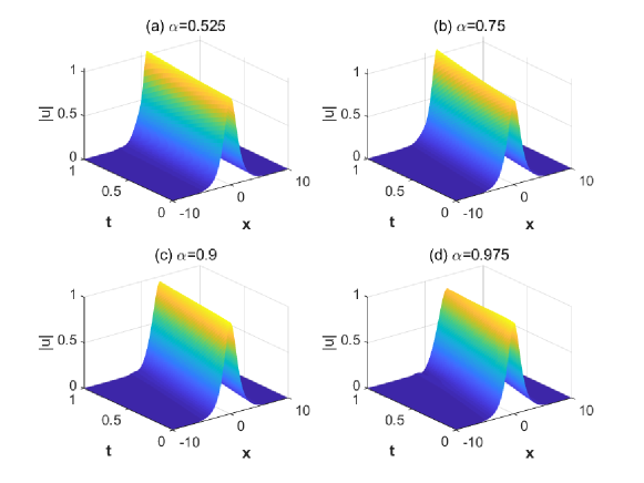
Figure 1: The evolution of the solution $|u(x,t)|$ with the initial condition $u(x,0)=\mathrm{sech}(x)\mathrm{exp}(2ix)$, where $\epsilon=0$, $\sigma=1$ and different $\alpha=0.525,0.75,0.9,0.975$.

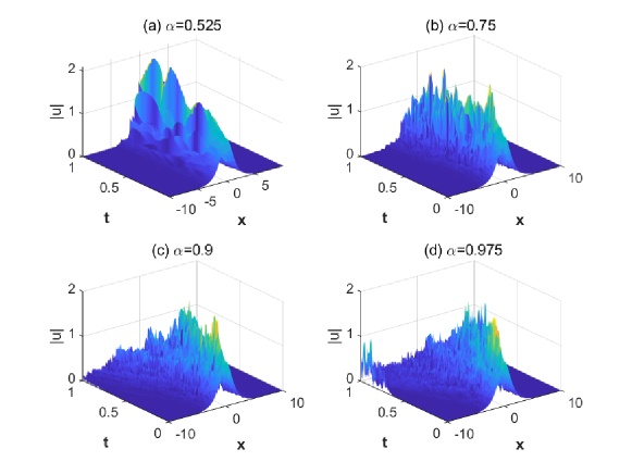
Figure 2: The evolution of the solution $|u(x,t)|$ with the initial condition $u(x,0)=\mathrm{sech}(x)\mathrm{exp}(2ix)$, where $\epsilon=1$, $\sigma=1$ and different $\alpha=0.525,0.75,0.9,0.975$.

6 Appendix A. Further Proofs.

6.1 Proof of Proposition 1.

Proof.

We prove Proposition 1 by the following three steps.
Step 1. Set

$$\mathcal{T}u(t):= S(t)u_{0}+i\int_{0}^{t}S(t-s)\left(\theta_{R}\left(|u|_{L^{\gamma}\left(0,s;L_{x}^{q}\right)}\right)|u(s)|^{2\sigma}u(s)\right)ds$$ (6.1)

$$-i\int_{0}^{t}S(t-s)(u(s)dW(s))-\frac{1}{2}\int_{0}^{t}S(t-s)\left(u(s)F_{\Phi}\right)ds,$$

$$\Lambda g(t):= \int_{0}^{t}S(t-s)g(s)ds,~{}~{}\mathcal{X}_{T}:=L^{\rho}\left(\Omega;\mathcal{C}\left([0,T];L^{2}\left(\mathbb{R}^{n}\right)\right)\cap L^{r}\left(0,T;L^{p}\left(\mathbb{R}^{n}\right)\right)\right).$$

For sufficiently small $T$, we will show that $\mathcal{T}$ is a contraction mapping in $\mathcal{X}_{T}$.

Let $u_{1},u_{2}\in\mathcal{X}_{T}$ be adapted processes. By Lemma 1 for the operator $S(t)$, we have

$$\left|\mathcal{T}u_{1}-\mathcal{T}u_{2}\right|_{L^{r}\left(0,T;L_{x}^{p}\right)} \leq C\left|\theta_{R}\left(\left|u_{1}\right|_{L^{\gamma}\left(0,t,L_{x}^{q}\right)}\right)\left|u_{1}\right|^{2\sigma}u_{1}-\theta_{R}\left(\left|u_{2}\right|_{L^{\gamma}\left(0,t,L_{x}\right)}\right)\left|u_{2}\right|^{2\sigma}u_{2}\right|_{L^{\gamma^{\prime}}\left(0,T,L_{x}^{q^{\prime}}\right)}$$ (6.2)

$$+\left|\int_{0}^{t}S(t-s)\left(\left(u_{1}(s)-u_{2}(s)\right)dW(s)\right)\right|_{L^{r}\left(0,T;L_{x}^{p}\right)}\quad+C\left|\left(u_{1}-u_{2}\right)F_{\Phi}\right|_{L^{r^{\prime}}\left(0,T;L_{x}^{p^{\prime}}\right)}$$

$$:=J_{1}+J_{2}+J_{3},$$

where $r^{\prime},p^{\prime},\gamma^{\prime},q^{\prime}$, are respectively conjugates of $r,p,\gamma,q$. Note that $(r,p)$ and $(\gamma,q)$ are admissible pairs.

For the term $J_{1}$, using the similar technique as [11, Lemma 3.2], we have

$$J_{1}\leq C_{R}T^{1-n\sigma/2}\left|u_{1}-u_{2}\right|_{L^{\gamma}\left(0,T;L_{x}^{q}\right)}.$$ (6.3)

For the term $J_{3}$, by Hölder inequality for the variables $x$ and $t$, respectively, we obtain

$$J_{3}\leq C|u_{1}-u_{2}|_{L^{r^{\prime}}(0,T;L^{p}_{x})}|F_{\Phi}|_{L_{x}^{\frac{nr}{4\alpha}}}\leq CT^{1-\frac{2}{r}}|u_{1}-u_{2}|_{L^{r}(0,T;L^{p}_{x})}\left|F_{\Phi}\right|_{L_{x}^{\frac{nr}{4\alpha}}}.$$

Note that $\Phi$ is Hilbert-Schmidt in $L^{2}\left(\mathbb{R}^{n},\mathbb{R}\right)$, it is given by a kernel $k(x,y)\in L^{2}\left(\mathbb{R}^{n}\times\mathbb{R}^{n},\mathbb{R}\right)$:

$$\Phi h(x)=\int_{\mathbb{R}^{n}}k(x,y)h(y)dy,\quad\forall h\in L^{2}\left(\mathbb{R}^{n}\right).$$

Thus by Remark 3.2 in [30] and the Plancherel identity, we have

$$|k(x,y)|_{L_{x}^{\frac{nr}{2\alpha}}\left(L_{y}^{2}\right)}\leq C\|\Phi\|_{R\left(L_{x}^{2};L_{x}^{\frac{nr}{2\alpha}}\right)},$$

$$|k(x,\cdot)|_{L_{y}^{2}}^{2} =\sum_{\ell=0}^{\infty}\left(\int_{\mathbb{R}^{n}}k(x,y)e_{\ell}(y)dy\right)^{2}=\sum_{\ell=0}^{\infty}\left(\Phi e_{\ell}\right)^{2}(x)=F_{\Phi}(x),$$

and

$$\left|F_{\Phi}\right|_{L_{x}^{\frac{nr}{4\alpha}}}=|k(x,y)|_{L_{x}^{\frac{nr}{2\alpha}}\left(L_{y}^{2}\right)}^{2}\leq C\|\Phi\|_{R\left(L_{x}^{2};L_{x}^{\frac{nr}{2\alpha}}\right)}^{2}\leq C\left(\|\Phi\|_{L_{2}^{0}\left(L_{x}^{2}\right)}^{2}+\|\Phi\|_{R\left(L_{x}^{2};L_{x}^{2+\delta}\right)}^{2}\right).$$

Therefore we have

$$J_{3}\leq CT^{1-\frac{2}{r}}\left(\|\Phi\|_{L_{2}^{0}\left(L_{x}^{2}\right)}^{2}+\|\Phi\|_{R\left(L_{x}^{2};L_{x}^{2+\delta}\right)}^{2}\right)\left|u_{1}-u_{2}\right|_{L^{r}\left(0,T;L_{x}^{p}\right)}.$$ (6.4)

Taking the inequalities (6.3) and (6.4) into (6.2), and using Corollary 1, we get for any $\rho\geq r$,

$$\begin{aligned} \left|\mathcal{T}u_{1}-\mathcal{T}u_{2}\right|_{L_{\omega}^{\rho}\left(L^{r}\left(0,T;L_{x}^{p}\right)\right)}&\leq C_{R}T^{1-n\sigma/2}\left|u_{1}-u_{2}\right|_{L^{\gamma}\left(0,T;L_{x}^{q}\right)}\\ &+C\left(\|\Phi\|_{L_{2}^{0}}+\|\Phi\|_{R\left(L_{x}^{2};L_{x}^{2+\delta}\right)}\right)T^{1/2-2/r}\left|u_{1}-u_{2}\right|_{L_{\omega}^{\rho}\left(L^{\infty}\left(0,T;L_{x}^{2}\right)\right)}\\ &+C\left(\|\Phi\|_{L_{2}^{0}}^{2}+\|\Phi\|_{R\left(L_{x}^{2};L_{x}^{2+\delta}\right)}^{2}\right)T^{1-2/r}\left|u_{1}-u_{2}\right|_{L_{\omega}^{\rho}\left(L^{r}\left(0,T;L_{x}^{p}\right)\right)}.\end{aligned}.$$

Interpolating $L^{\gamma}\left(0,T;L^{q}\left(\mathbb{R}^{n}\right)\right)$ between $L^{\infty}\left(0,T;L^{2}\left(\mathbb{R}^{n}\right)\right)$ and $L^{r}\left(0,T;L^{p}\left(\mathbb{R}^{n}\right)\right)$, and assuming that $T\leq T_{0}$, we finally obtain

$$\left|\mathcal{T}u_{1}-\mathcal{T}u_{2}\right|_{L_{\omega}^{\rho}\left(L^{r}\left(0,T;L^{p}\left(\mathbb{R}^{n}\right)\right)\right)} \leq C\left(R,T_{0},\|\Phi\|_{L_{2}^{0},}\|\Phi\|_{R\left(L_{x}^{2};L_{x}^{2+\delta}\right)}\right)T^{\frac{1}{2}-\frac{1}{r}}\left|u_{1}-u_{2}\right|_{\mathcal{X}_{T}}.$$

Step 2. Let $u_{1},u_{2}$ be adapted and in $X_{T}$, by using the same technique as step 1 with $L^{r}\left(0,T;L_{x}^{p}\right)$ replaced by $L^{\infty}\left(0,T;L_{x}^{2}\right)$ and Lemma 4, we have

$$\left|\mathcal{T}u_{1}-\mathcal{T}u_{2}\right|_{L_{\omega}^{\rho}\left(L^{\infty}\left(0,T;L_{x}^{2}\right)\right)}\leq C\left(R,T_{0},\|\Phi\|_{L_{2}^{0}},\|\Phi\|_{R\left(L_{x}^{2};L_{x}^{2+\delta}\right)}\right)T^{\frac{1}{2}-\frac{1}{r}}\left|u_{1}-u_{2}\right|_{\mathcal{X}_{T}}.$$ (6.5)

Step 3. Taking $T\leq\inf\left(T_{0},\frac{1}{\left(2C(T_{0},\|\Phi\|_{L_{2}^{0}},\|\Phi\|_{R(L_{x}^{2},L_{x}^{2+\delta})})\right)^{2r/(r-2)}}\right)$, we know $\mathcal{T}$ is a contraction mapping in $X_{T}$. By Banach’s fixed-point theorem, the map $\mathcal{T}$ has a unique fixed point in $X_{T}$, which is the unique solution of (6.1). Moreover, the solution may be extended to the whole interval $\left[0,T_{0}\right]$. ∎

6.2 Proof of Proposition 2.

Proof.

We recall that $u_{m}$ satisfies the integral Eq. (3.5), which is the mild form of the following Itô’s equation,

$$idu-\left((-\Delta)^{\alpha}u-\theta_{m}\left(|u|_{L^{\gamma}\left(0,t;L_{x}^{q}\right)}\right)|u|^{2\sigma}u\right)dt=udW-\frac{i}{2}uF_{\Phi}dt,~{}~{}u_{m}(0)=u_{0}.$$ (6.6)

Applying Itô formula to the functional $\left|u_{m}(t)\right|_{L^{2}\left(\mathbb{R}^{n}\right)}^{2}$ and $\Phi$ is real valued, we get

$$\left|u_{m}(t)\right|_{L_{x}^{2}}^{2}= \left|u_{0}\right|_{L_{x}^{2}}^{2}+2\rm{Im}\int^{t}_{0}\left((-\Delta)^{\alpha}u_{m},u_{m}\right)ds-2\rm{Im}\int_{0}^{t}\left(\theta_{m}\left(\left|u_{m}\right|_{L^{\gamma}\left(0,s;\left(L_{x}^{q}\right)\right)}\right)\left|u_{m}\right|^{2\sigma}u_{m},u_{m}\right)ds$$ (6.7)

$$+2\rm{Im}\sum_{k=0}^{\infty}\int_{0}^{t}\left(u_{m}\Phi e_{k},u_{m}\right)d\beta_{k}-\rm{Re}\int_{0}^{t}\left(u_{m}\sum_{k=0}^{\infty}\left(\Phi e_{k}\right)^{2},u_{m}\right)ds+\int_{0}^{t}\sum_{k=0}^{\infty}\left|u_{m}\Phi e_{k}\right|_{L_{x}^{2}}^{2}ds$$

$$= \left|u_{0}\right|_{L_{x}^{2}}^{2}.$$

Next, applying the Strichartz inequality to the integral Eq. (3.5) and using a regularization procedure, we obtain

$$\left|u_{m}\right|_{L^{r}\left(0,T;L_{x}^{p}\right)}\leq C\left|u_{0}\right|_{L_{x}^{2}}+C\left|\theta_{m}\left(\left|u_{m}\right|_{L^{\gamma}\left(0,t;L_{x}^{q}\right)}\right)\left|u_{m}\right|^{2\sigma}u_{m}\right|_{L^{\gamma}\left(0,T;L_{x}^{q^{\prime}}\right)}$$

$$+\left|Ju_{m}\right|_{L^{r}\left(0,T;L_{x}^{p}\right)}+C\left|u_{m}F_{\Phi}\right|_{L^{r^{\prime}}\left(0,T;L_{x}^{p^{\prime}}\right)}$$

$$\leq C_{1}\left|u_{0}\right|_{L_{x}^{2}}+C_{2}T^{1-\frac{n\sigma}{2\alpha}}\left|u_{m}\right|_{L^{\gamma}\left(0,T;L_{x}^{q}\right)}^{2\sigma+1}$$

$$+C_{3}T^{1-2/r}\left(\|\Phi\|_{L_{2}^{0}}^{2}+\|\Phi\|_{R\left(L_{x}^{2};L_{x}^{2+\delta}\right)}^{2}\right)\left|u_{m}\right|_{L^{r}\left(0,T;L_{x}^{p}\right)}+\left|Ju_{m}\right|_{L^{r}\left(0,T;L_{x}^{p}\right)}.$$

Now, we assume that $T\leq T_{1}$ with $C_{3}T_{1}^{1-2/r}\left(\|\Phi\|_{L_{2}^{0}}^{2}+\|\Phi\|_{R\left(L_{x}^{2};L_{x}^{2+\delta}\right)}^{2}\right)=\frac{1}{2}$, so that the preceding estimate leads to

$$\left|u_{m}\right|_{L^{r}\left(0,T;L_{x}^{p}\right)}\leq 2C_{1}\left|u_{0}\right|_{L_{x}^{2}}+2C_{2}T^{1-\frac{n\sigma}{2\alpha}}\left|u_{m}\right|_{L^{\gamma}\left(0,T;L_{x}^{q}\right)}^{2\sigma+1}+2\left|Ju_{m}\right|_{L^{r}\left(0,T_{0};L_{x}^{p}\right)}.$$

Let $\theta$ be such that $\frac{1}{q}=\frac{\theta}{2}+\frac{1-\theta}{p}$, then interpolating $L^{\gamma}\left(0,T;L_{x}^{q}\right)$ between $L^{\infty}\left(0,T;L_{x}^{2}\right)$ and $L^{r}\left(0,T;L_{x}^{p}\right)$, and using the fact that $\left|u_{m}\right|_{L^{\infty}\left(0,T;L_{x}^{2}\right)}=$ $\left|u_{0}\right|_{L_{x}^{2}}$ and Young’s inequality, we see that if $T\leq\inf\left(T_{0},T_{1}\right)$

$$\left|u_{m}\right|_{L^{r}\left(0,T;L_{x}^{p}\right)} \leq 2C_{1}\left|u_{0}\right|_{L_{x}^{2}}+2\left|Ju_{m}\right|_{L^{r}\left(0,T_{0};L_{x}^{p}\right)}+2C_{2}T^{1-\frac{n\sigma}{2\alpha}}\left|u_{0}\right|_{L_{x}^{2}}^{\theta(2\sigma+1)}\left|u_{m}\right|_{L^{r}\left(0,T;L_{x}^{p}\right)}^{(1-\theta)(2\sigma+1)}$$

$$\leq C_{4}\left(T_{0}\right)\left|u_{0}\right|_{L_{x}^{2}}\left(1+\left|u_{0}\right|_{L_{x}^{2}}^{2\sigma+1}\right)+2\left(\left|Ju_{m}\right|_{L^{r}\left(0,T_{0};L_{x}^{p}\right)}+\sup_{0\leq t_{0}\leq T_{0}}\left|Iu_{m}\left(t_{0},\cdot\right)\right|_{L^{r}\left(0,T_{0};L_{x}^{p}\right)}\right)$$

$$+T^{1-\frac{n\sigma}{2\alpha}}\left|u_{m}\right|_{L^{r}\left(0,T;L_{x}^{p}\right)}^{2\sigma+1}.$$

Set

$$K_{m}(\omega)= C_{4}\left(T_{0}\right)\left|u_{0}\right|_{L_{x}^{2}}\left(1+\left|u_{0}\right|_{L_{x}^{2}}^{2\sigma+1}\right)+2\left(\left|Ju_{m}\right|_{L^{r}\left(0,T_{0};L_{x}^{p}\right)}+\sup_{0\leq t_{0}\leq T_{0}}\left|Iu_{m}\left(t_{0},\cdot\right)\right|_{L^{r}\left(0,T_{0};L_{x}^{p}\right)}\right).$$ (6.8)

For all $T\leq\inf\left(T_{0},T_{1}\right)$, we have

$$\left|u_{m}\right|_{L^{r}\left(0,T;L_{x}^{p}\right)}\leq K_{m}(\omega)+T^{1-\frac{n\sigma}{2\alpha}}\left|u_{m}\right|_{L^{r}\left(0,T;L_{x}^{p}\right)}^{2\sigma+1}.$$

It follows that for $T$ small enough, we have $\left|u_{m}\right|_{L^{r}\left(0,T;L_{x}^{p}\right)}\leq 2K_{m}(\omega)$.

We may now reiterate the previous process on each interval $[jT,(j+1)T]\subset\left[0,T_{0}\right]$. Using the integral equation

$$u_{m}(t)= S(t-jT)u_{m}(jT)-i\int_{jT}^{t}S(t-s)\left(\theta_{m}\left(\left|u_{m}\right|_{L^{\gamma}\left(0,s;L_{x}^{q}\right)}\right)\left|u_{m}\right|^{2\sigma}u_{m}\right)ds$$

$$-i\int_{jT}^{t}S(t-s)\left(u_{m}(s)dW(s)\right)-\frac{1}{2}\int_{jT}^{t}S(t-s)\left(u_{m}(s)F_{\Phi}\right)ds.$$

By the same computations as before, we easily get

$$\left|u_{m}\right|_{L^{r}\left(jT,(j+1)T;L_{x}^{p}\right)} \leq 2C_{1}\left|u_{0}\right|_{L_{x}^{2}}+2\sup_{0\leq t_{0}\leq T_{0}}\left|\int_{t_{0}}^{t}S(t-s)\left(u_{m}(s)dW(s)\right)\right|_{L^{r}\left(t_{0},T_{0};L_{x}^{p}\right)}$$

$$+2C_{2}T^{1-\frac{n\sigma}{2\alpha}}\left|u_{0}\right|_{L_{x}^{2}}^{\theta(2\sigma+1)}\left|u_{m}\right|_{L^{r}\left(jT,(j+1)T;L_{x}^{p}\right)}^{(1-\theta)(2\sigma+1)}.$$

Now, using the trivial fact that

$$\int_{t_{0}}^{t}S(t-s)\left(u_{m}(s)dW(s)\right)=\int_{0}^{t}S(t-s)\left(u_{m}(s)dW(s)\right)-\int_{0}^{t_{0}}S(t-s)\left(u_{m}(s)dW(s)\right),$$

we have

$$\sup_{0\leq t_{0}\leq T_{0}}\left|\int_{t_{0}}^{t}S(t-s)\left(u_{m}(s)dW(s)\right)\right|_{L^{r}\left(t_{0},T_{0};L_{x}^{p}\right)}\leq\left|Ju_{m}\right|_{L^{r}\left(0,T_{0};L_{x}^{p}\right)}+\sup_{0\leq t_{0}\leq T_{0}}\left|Iu_{m}\left(t_{0},\cdot\right)\right|_{L^{r}\left(0,T_{0};L_{x}^{p}\right)}.$$

Therefore we see that $\left|u_{m}\right|_{L^{r}\left(jT,(j+1)T;L_{x}^{p}\right)}\leq 2K_{m}(\omega)$ for each $j$ such that $[jT,(j+1)T]\subset\left[0,T_{0}\right]$, and where $K_{m}(\omega)$ is defined in (6.8). As a consequence, we have,

$$\left|u_{m}\right|_{L^{r}\left(0,T_{0};L_{x}^{p}\right)} \leq\sum_{j}\left|u_{m}\right|_{L^{r}\left(jT,(j+1)T;L_{x}^{p}\right)}\leq 2\left(\frac{T_{0}}{T}+1\right)K_{m}(\omega)\leq{C_{5}}(T_{0})K_{m}+{C_{6}}(T_{0})K_{m}^{\frac{4\sigma}{2\alpha-n\sigma}+1}.$$

Hence, if $\rho\geq(2\sigma+2)\left(\frac{4\sigma}{2\alpha-n\sigma}+1\right)$, and using Hölder inequality, we get

$$\mathbb{E}\left(\left|u_{m}\right|_{L^{r}\left(0,T_{0};L_{x}^{p}\right)}\right)\leq C_{T_{0}}\left\{\mathbb{E}\left|u_{0}\right|_{L_{x}^{2}}^{\rho}+\mathbb{E}\left(\left|Ju_{m}\right|_{L^{r}\left(0,T_{0};L_{x}^{p}\right)}^{\rho}\right)+\mathbb{E}\left(\sup_{0\leq t_{0}\leq T_{0}}\left|Iu_{m}\left(t_{0},\cdot\right)\right|_{L^{r}\left(0,T_{0};L_{x}^{p}\right)}^{\rho}\right)\right\},$$

and

$$\mathbb{E}\left(\sup_{0\leq t_{0}\leq T_{0}}\left|Iu_{m}\left(t_{0},\cdot\right)\right|_{L^{r}\left(0,T_{0};L_{x}^{p}\right)}^{\rho}\right) \leq T_{0}^{\rho/r-1}\mathbb{E}\left(\int_{0}^{T_{0}}\sup_{0\leq t_{0}\leq T_{0}}\left|Iu_{m}\left(t_{0},t\right)\right|_{L_{x}^{p}}^{\rho}dt\right)$$

$$\leq CT_{0}^{\rho/r}\left(\|\Phi\|_{L_{2}^{0}}+\|\Phi\|_{R\left(L_{x}^{2},L_{x}^{2+\delta}\right)}\right)^{\rho}T_{0}^{\rho\left(\frac{1}{2}-\frac{2}{r}\right)}\mathbb{E}\left(\left|u_{m}\right|_{L^{\infty}\left(0,T_{0};L_{x}^{2}\right)}^{\rho}\right).$$

The same bound is true for $\mathbb{E}\left(\left|Ju_{m}\right|_{L^{r}\left(0,T_{0};L_{x}^{p}\right)}^{\rho}\right)$ by Corollary 1. By the fact that $\left|u_{m}\right|_{L^{\infty}\left(0,T_{0};L_{x}^{2}\right)}=\left|u_{0}\right|_{L_{x}^{2}}$ for a.e. $\omega\in\Omega$, we obtain

$$\mathbb{E}\left(\left|u_{m}\right|_{L^{r}\left(0,T_{0};L_{x}^{p}\right)}\right)\leq C_{T_{0}}\mathbb{E}\left(\left|u_{0}\right|_{L_{x}^{2}}^{\rho}\right)\left(1+\|\Phi\|_{L_{2}^{0}}+\|\Phi\|_{R\left(L_{x}^{2},L_{x}^{2+\delta}\right)}\right)^{\rho}.$$

∎

7 Acknowledgments

The authors would like to thank Qi Zhang (Yau Mathematical Sciences Center, Tsinghua University), Yongsheng Li (South China University of Technology), and Jianglun Wu (Beijing Normal University-Hong Kong Baptist University United International College) for their helpful discussions. The research of X. Wang is supported by the Natural Science Foundation of Henan Province of China (Grant No. 232300420110). The research of Z. Wang was supported by the NSFC grant. 11531006 and 11771449.

References

[1]
S. Longhi,
Fractional Schrödinger equation in optics,
Optics Letters, 40: 1117-1120, 2015.
[2]
S. Liu, Y. Zhang, B. A. Malomed, E. Karimi,
Experimental realisations of the fractional
Schrödinger equation in the temporal domain,
Nature Communications, 14: 222, 2023.
[3]
A. D. Ionescu, F. Pusateri,
Nonlinear fractional Schrödinger equations in one dimension,
Journal of Functional Analysis, 266: 139-176, 2014.
[4]
N. Laskin,
Fractional Schrödinger equation,
Physical Review E, 66: 056108, 2002.
[5]
K. Kirkpatrick, E. Lenzmann, G. Staffilani,
On the continuum limit for discrete NLS with long-range lattice interactions,
Physical Review E, 66: 056108, 2002.
[6]
B. Guo, D. Huang,
Existence and stability of standing waves for nonlinear fractional Schrödinger equations,
Journal of Mathematical Physics, 53: 083702, 2012.
[7]
X. Shang, J. Zhang,
Ground states for fractional Schrödinger equation with critical growth,
Nonlinearity, 27: 187-207, 2014.
[8]
B. Choi, A. Ceves,
Continuum limit of fractional nonlinear Schrödinger equation,
Journal of Evolution Equations, 23: 30, 2023.
[9]
R. L. Frank, E. Lenzmann, L. Silvestre,
Uniqueness of radial solutions for the fractional Laplacian,
Communications on Pure and Applied Mathematics, 69: 1671-1726, 2016.
[10]
P. Wang, C. Huang,
An energy conservative difference scheme for the nonlinear fractional Schrödinger equations,
Journal of Computational Physics, 293: 238-251, 2015.
[11]
A. de Bouard, A. Debussche,
A stochastic nonlinear Schrödinger equation with multiplicative noise,
Communications in Mathematical Physics, 205: 121-127, 1999.
[12]
A. de Bouard, A. Debussche,
Blow-up for the stochastic nonlinear Schrödinger equation with multiplicative noise,
The Annals of Probability, 33: 1078-1110, 2005.
[13]
S. Herr, M. Röckner, D. Zhang,
Scatter for stochastic nonlinear Schrödinger equations,
Communications in Mathematical Physics, 368: 843-884, 2019.
[14]
V. Barbu, M. Röckner, D. Zhang,
Stochastic nonlinear Schrödinger equations: No blow-up in the non-conservative case,
Journal of Differential Equations, 263: 7919-7940, 2017.
[15]
A. Debussche, L. D. Menza,
Numerical simulation of focusing stochastic nonlinear Schrödinger equations,
Physica D, 162: 131-154, 2002.
[16]
Z. Brzeźniak, W. Liu, J. Zhu,
The stochastic Strichartz estimates and stochastic nonlinear Schrödinger equations driven by Lévy noise,
Journal of Functional Analysis, 281: 109021, 2021.
[17]
Y. Deng, A. R. Nahmod, H. Yue,
Random tensors, propagation of randomness, and nonlinear dispersive equations,
Inventiones Mathematicae, 228: 539-686, 2022.
[18]
J. Cui, J. Hong, Z. Liu, W. Zhou,
Strong convergence rate of splitting schemes for stochastic nonlinear Schrödinger equations,
Journal of Differential Equations, 266: 5625-5663, 2019.
[19]
H. Yuan, G. Chen,
Martingale solutions of stochastic fractional nonlinear Schrödinger equation on a bounded interval,
Journal of Differential Equations, 263: 7919-7940, 2017.
[20]
V. D. Dinh,
On blow-up solutions to the focusing mass-critical nonlinear fractional schrödinger equation,
Communication on Pure and Applied Analysis, 18: 689-708, 2019.
[21]
T. Boulenger, D. Himmelsbach, E. Lenzmann,
Blowup for fractional NLS,
Journal of Functional Analysis, 271: 2569-2603, 2016.
[22]
S. Zhu,
On the blow-up solutions for the nonlinear fractional Schrödinger equation,
Journal of Differential Equations, 261: 1506-1531, 2016.
[23]
Q. Guo, S. Zhu,
Sharp threshold of blow-up and scattering for the fractional Hartree equation,
Journal of Differential Equations, 264: 2802-2832, 2018.
[24]
V. Barbu, M. Röckner, D. Zhang,
Stochastic nonlinear Schrödinger equations: No blow-up in the non-conservative case,
Applicable Analysis, 96: 2553-2574, 2017.
[25]
Y. Lan,
Blow-up Dynamics for -critical fractional Schrödinger equations,
International Mathematics Research Notices, 18: 13753-13810, 2022.
[26]
Y. Cho, G. Hwang, S. Kwon, et al.,
Well-posedness and ill-posedness for the cubic fractional Schrödinger equations,
Discrete and Continuous Dynamical Systems, 35: 2863-2880, 2015.
[27]
N. N. Vakhania, V. I. Taireladze, S. A. Chobanyan,
Probability and distribution on Banach space,
Springer Science Business Media, 1987.
[28]
E. Di Nezza, G. Palatucci, E. Valdinoci,
Hitchhiker’s guide to the fractional Sobolev spaces,
Bulletin des Sciences Mathématiques, 136: 521-573, 2012.
[29]
V. D. Dinh,
A study on blowup solutions to the focusing -supercritical nonlinear fractional Schrödinger equation,
Journal of Mathematical Physics, 59: 071506, 2018.
[30]
Z. Brzeźniak, S. Peszat,
Space-time continuous solutions to SPDE’s driven by a homogeneous Wiener process,
Studia Mathematica, 137: 261-299, 1999.