Domain Reduction Strategy for Non Line of Sight Imaging

Abstract

This paper presents a novel optimization-based method for non-line-of-sight (NLOS) imaging that aims to reconstruct hidden scenes under various setups. Our method is built upon the observation that photons returning from each point in hidden volumes can be independently computed if the interactions between hidden surfaces are trivially ignored. We model the generalized light propagation function to accurately represent the transients as a linear combination of these functions. Moreover, our proposed method includes a domain reduction procedure to exclude empty areas of the hidden volumes from the set of propagation functions, thereby improving computational efficiency of the optimization. We demonstrate the effectiveness of the method in various NLOS scenarios, including non-planar relay wall, sparse scanning patterns, confocal and non-confocal, and surface geometry reconstruction. Experiments conducted on both synthetic and real-world data clearly support the superiority and the efficiency of the proposed method in general NLOS scenarios.

1 Introduction

The ability to see the objects placed over the direct line-of-sight has the potential to benefit various applications, e.g. autonomous driving, medical care, rescue operations and robotics. The task, known as non-line-of-sight (NLOS) imaging, reconstructs hidden scenes from measurements of indirect reflections. These transient measurements are commonly obtained via ”looking around the corner”, where a light source and a high-resolution time-of-flight sensor illuminate and scan the relay wall (Figure 1 a). Hidden objects are then reconstructed from captures of the multi-bounce returning photons using appropriate computing algorithms.

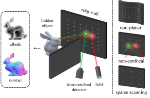
Figure 1: A common NLOS scanning system. A laser and a time-resolved sensor illuminate and scan the relay wall to capture the transients. Our method can reconstruct both albedo and surface normal of the hidden objects in general scenarios, including non-confocal, planar relay walls and sparse scanning.

Recent advancements in NLOS imaging have been achieved by methods that directly solve the inverse problem. Such inverse methods include back-projection [29], 3D convolution based solutions [21, 31, 1], wave-based Stolt migration [14], and phasor field methods based on diffraction [18, 17]. Despite promising results, one or more assumptions are made to model the exact solutions, such as a diffuse and planar relay wall or a certain scanning system. In addition, raster scanning of the relay wall is required for these methods to reconstruct the high-resolution outputs [1], which is time-consuming to be applied in practice.

Considering the practical applications of NLOS imaging, there are numerous scenarios where the exact solutions may not be sufficient to meet the demands. In many cases, it may be necessary to reconstruct more accurate surface geometry, the ideal relay wall may not exist and raster scanning of the relay wall may not be feasible. These real-world situations give rise to the need for solutions that can solve NLOS imaging under more general settings. Several works have made the efforts to meet this demand and presented optimization-based NLOS methods [8, 28, 25, 22]. While they are more generally applicable than exact solutions, massive computations per iteration are required for them, most of which are assigned for the unoccupied and unnecessary parts of the hidden volumes.

In this paper, we present a novel optimization-based method for NLOS imaging that can reconstruct hidden scenes in more practical scenarios. Our method is built upon the fundamental observation that photons returning from each point in hidden volumes can be independently computed, if the trivial effects of interactions between hidden surfaces are ignored. We begin by modeling the generalized light propagation function, which maps albedo and surface normal to the transient space with various types of relay walls and scanning environments. With accurately modeled scene-invariant propagation functions, the transients can be represented as a superposition of these functions. We aim to reconstruct the hidden volumes by finding the corresponding albedo and normal of each function. Different from [22], where the similar observation was exploited as a matrix form of point spread function [22], our propagation functions accurately model several fall-off terms which are ignored in [22], and are computed with a continuously sampled points set. As a result, our method is able to accurately reconstruct the surface geometry as well as the albedo.

Representing transients as a superposition allows more efficient computation. Here, we propose a domain reduction procedure to accomplish such efficiency, by distinguishing empty areas of the hidden volumes and gradually excluding them from the set of propagation functions. It is worth mentioning that in NLOS problems, visible surfaces of the target objects occupy less than 5% regions of the entire hidden space. Other empty regions do not actually contribute to both transients and the reconstruction volumes. Our domain reduction strategy periodically identifies and prunes these unnecessary computations, significantly boosting the efficiency of the optimization process. This domain reduction procedure is conducted in a coarse-to-fine manner, which enables our method to reconstruct the high-resolution output volumes with a single commercial GPU.

We demonstrate the validity of our method under various NLOS scenarios, including non-planar relay wall, sparse scanning patterns, confocal and non-confocal, and surface geometry reconstruction (Figure 1 (b)). The experiment results conducted on both synthetic [6] and real-world inputs [14] support that our method can efficiently reconstruct the hidden objects with fine details under more generalized and real-world applicable scenarios.

2 Related work

NLOS imaging. NLOS imaging was first introduced by Kirmani et al. [13], and experimentally validated in [29] by using a femtosecond laser and a streak camera. Various methods have been developed for NLOS imaging, which can be broadly divided into two parts: active [21, 14, 10, 27, 9] and passive methods [24, 26, 23, 4, 3, 30]. Active NLOS methods utilize controllable light sources and time-of-flight detectors, whereas passive methods rely on indirect light. Since time-resolved detectors provide transient measurements containing abundant information, active NLOS methods tend to produce higher-quality results. In the active NLOS setup, the pulsed laser emits photons to the visible wall and measures the amount of returning photons to reveal the shape of the hidden object. The reconstruction quality of active NLOS imaging has been rapidly developing, and the reconstructed outputs have also been diversified such as albedo [21, 1], normal [31, 7], surface [28] and depth [5].

Inverse NLOS methods. Recently, significant development has been made in NLOS imaging through various exact solutions. By assuming isotropic light scatters and planar relay wall, O’Toole et al. [21] demonstrated that the NLOS imaging problem can be interpreted as a 3D deconvolution problem under the confocal scanning setup and proposed the light-cone transform (LCT) method. Their main concept is further extended by Young et al. [31], where the method named DLCT was proposed to obtain the surface normal as well as the albedo using a vector deconvolution. Lindell et al. [14] interpreted NLOS imaging as a boundary value problem and presented a wave-based solution named f-k migration. Phasor field methods [18, 17] formulated the NLOS imaging problem as a diffractive wave propagation and solved the Rayleigh-Sommerfeld integral to recover the hidden objects. While these exact solutions produced impressive results, they require several assumptions and constraints, e.g. planar relay wall, specific (confocal or non-confocal) scanning system and exhaustive raster scanning for high-resolution outputs. In addition, methods except DLCT [31] can only reconstruct the albedo of the hidden scenes. Although such constraints allow faster computations, general applicability and accurate surface modeling of these inverse methods remains challenges.

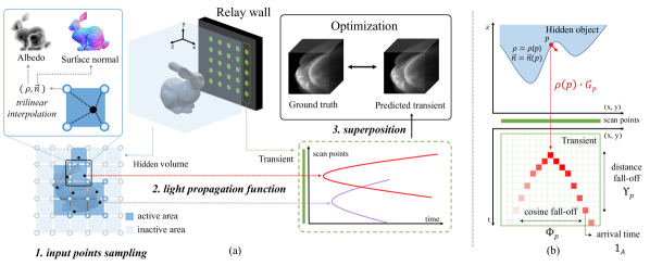
Figure 2: (a) The overview of our proposed training scheme. We divide hidden space to grid shape and assign albedo $\rho$ and surface normal $\vec{n}$ for each vertex. Input points are randomly sampled from the hidden space. Then the light propagation from each point $G_{p}$ is computed, of which superposition is used as predicted transients. The variables are optimized by minimizing the L2 distance. Our domain is gradually reduced by pruning the empty regions during the optimization. (b) The computation of light propagation function from each point $p$. The arrival time at scan point $s$ is first identified, and then the fall-off terms $\Phi_{p}$ and $\Upsilon_{p}$ are computed using $p$, $l$, $s$ and $\vec{n}(p)$.

NLOS methods for general setups. To address the challenges of recovering hidden objects in more challenging real-world situations, several approximate, iterative and optimization-based methods have also been proposed. Back-projection based solvers [29, 2, 1] are one of the commonly used techniques for general NLOS imaging. Ahn et al. [1] proposed the iterative deconvolution-based approach that can operate without being bounded to a certain scan system and the lateral resolution of the transients. Heide et al. [8] proposed a volumetric-based optimization method that can handle partial occlusion and surface normal. The optimization-based method using a point spread function [22] was also proposed. Tsai et al. [28] proposed the surface optimization method that can reconstruct the continuous surfaces of the hidden scenes, of which results are sensitive to the initial state. NeTF [25] proposed neural representations similar to NeRF [20] for NLOS imaging, but their optimization time and blurry results limit its potentials. While they reconstruct the hidden scenes in general NLOS scenarios, most of them can only reconstruct the albedo and suffer from huge computational costs, usually $O(N^{5})$ or $O(N^{6})$ per iteration. We follow this line of work to accurately reconstruct the hidden volumes under the general NLOS setups, through the optimization with accurately modelled light propagation and the efficient computations with our domain reduction strategy.

3 Method

3.1 NLOS measurement model

We begin by formulating the transient imaging model for an arbitrary measurement environment, which relates the albedo and surface normal of the hidden objects to the measurements. In the active NLOS methods, the time-resolved sensor measures transients after light pulse is emitted onto the relay wall. Let $p$ be a point on surfaces of the hidden volumes which follows Lambert’s cosine law, and assume that there are no interactions between the surfaces (inter-reflections and self-occlusion). The measured transients can be formulated as

$$\;\tau(t,l,s)$$ (1)

$$=\int_{p\in\Omega}\rho(p)\cdot\Phi_{p}(l,\vec{n}(p))\cdot\Upsilon_{p}(l,s)\cdot\delta(d_{l}+d_{s}-tc)\;dp,$$

$$\quad\Phi_{p}(l,\vec{n}(p))=\langle{l-p\over||l-p||},\vec{n}(p)\rangle,\;\Upsilon_{p}(l,s)={1\over d_{l}^{2}}\cdot{1\over d_{s}^{2}},$$

where $l$ and $s$ represent the laser and scan point of the relay wall, and $\rho(p)$ and $\vec{n}(p)$ are the albedo and the surface normal of point $p$ on the hidden space $\Omega$. $\Phi_{p}(l,\vec{n})$ models the view-dependent cosine fall-off term along Lambert’s cosine law. $\Upsilon_{p}(l,s)$ models the distance fall-off, where $d_{l}$, $d_{s}$ are the distances from the hidden scene to the laser and the scan point respectively. The Dirac delta $\delta(\cdot)$ relates time to the light travel distance, $c$ is the speed of light and $t$ is the arrival time of photons. Note that our transient formation model is defined without assumptions on a relay wall and scanning setups. By additionally assuming a confocal scanning system and a planar relay wall, our formation model becomes equivalent to the formation model of DLCT [31].

Since each point $p$ in $\Omega$ independently contributes to the transients in our formation model, we can represent the transients as a superposition of functions that models the light propagation from each $p$. To decompose the transients into a set of functions, we first model the light propagation function for given $p$ as

$$g_{p}(t,l,s)=\Phi_{p}(l,\vec{n}(p))\cdot\Upsilon_{p}(l,s)\cdot\delta(d_{l}+d_{s}-tc).$$ (2)

The propagation function $g_{p}$ determines the arrival time and radiometric fall-off terms according to $l$ and $s$. It can be interpreted as a tailored point spread function that depends on $p$, $l$, $s$ and the surface normal $\vec{n}(p)$ at $p$. With the above equation, the entire transients can be expressed as

$$\tau=\int_{p\in\Omega}\rho(p)\ \cdot\ g_{p}\ dp.$$ (3)

Each $\rho(p)\cdot g_{p}$ represents 3D sub-signals containing all measured photons returning from point $p$. Our goal becomes revealing $\rho$ and $\vec{n}$ to $p$ that correspond to each decomposed function, without posing constraints on $l$, $s$ and without losing accurate modeling of light propagation.

3.2 Reconstruction by decomposition

By ignoring the radiometric fall-off terms $\Phi$ and $\Upsilon$, the above equation can be interpreted as an elliptical Radon transform [16]. It would enable easier approaches to find the inverse, but the accurate modeling would also be sacrificed. Therefore, we aim to reconstruct $\rho$ and $\vec{n}$ of the hidden volumes through the optimization, by decomposing the transients into a set of functions. Instead of using a discretized matrix, we leverage a points set that is continuously sampled from the hidden space, to decompose the transients into the continuously defined propagation functions.

Figure 2 (a) illustrates the overview of our proposed reconstruction scheme. We first divide the hidden space into a grid and assign 4-dimensional variables, albedo $\rho$ and normal $\vec{n}$ to each vertex of the grid. In each optimization step, input points are sampled from the hidden space. Then the light propagation of each point is computed, which are composed to obtain the transient predictions. The 4-dimensional variables are optimized using gradient descent by minimizing the difference between the synthesized transients and the ground truth measurements. We illustrate the details of our optimization scheme in the following paragraphs.

Input points sampling.

Instead of using fixed points as inputs, we randomly sample the input points from the hidden space for every step. Such sampling procedure enables the variables to be optimized in a more continuous way. We utilize a grid-based random sampling technique to achieve spatially balanced points sampling. We sample one point from each grid bin, resulting in a set of points denoted as $H$. The albedo and normal at each point are determined by the trilinear interpolation of the surrounding 8 vertices.

Light propagation and superposition.

To synthesize the transients with a sampled points set $H$, we discretize the transients in Equation (3) to a finite linear combination of $\{G_{p}\}$, where $G_{p}$ can be expressed as

$$\begin{gathered}G_{p}=\Phi_{p}\cdot\Upsilon_{p}\cdot 1_{A},\cr A=\{(t,l,s)\;|\;d_{l}+d_{s}=tc\}.\end{gathered}$$ (4)

To compute $G_{p}$, we first identify the non-zero histograms of each scan point $s$ with given $l$ and $s$, by computing $t$ that satisfies the indicate function $1_{A}$. The contribution at the corresponding location is then determined by $\Phi_{p}$ and $\Upsilon_{p}$, which are calculated as in Figure 2 (b). Computations of light propagation are done in parallel for all points in $H$, and thus can be accelerated by GPU. Finally, we compute the predicted transients with a linear summation:

$$T=\sum_{p\in H}\rho(p)\cdot G_{p}\cdot\Delta V,$$ (5)

where $\Delta V$ is volume of a grid bin. We update $\rho$ and $\vec{n}$ at each vertex using the gradient descent, by minimizing the L2 distance between the rendered and the ground truth.

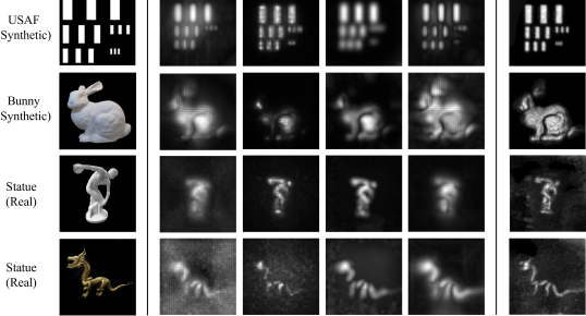
Figure 3: Reconstruction results on the transients with a confocal $32\times 32$ scan system and a planar relay wall.

3.3 Domain reduction strategy

One crucial observation is that most of the hidden volumes to reconstruct is empty in the NLOS imaging scenarios, since photons are only reflected from the visible surfaces of the objects. These empty regions do not actually affect either the measured transients or the reconstruction volumes. By taking the advantages of this sparsity nature, most of the computations in synthesizing transients can be eliminated, as our predicted transients are a linear sum of the propagation functions. The synthesized transients in Equation (5) can be divided as

$$\begin{gathered}T=\sum_{p\in\Omega_{1}}\rho(p)\cdot G_{p}\cdot\Delta V+\sum_{p\in\Omega_{2}}\rho(p)\cdot G_{p}\cdot\Delta V,\cr\Omega_{1}=\{\;p\in\Omega^{\prime}|\;\rho(p)>\epsilon\;\},\Omega_{2}=\Omega^{\prime}\setminus\Omega_{1},\end{gathered}$$ (6)

where $\Omega^{\prime}\subset\Omega$ is a set of points that corresponds to the vertices in the grids. Since the values in the summation are always positive, we can ignore the operations of the second term if $\epsilon$ is a sufficiently small value ($||\rho(p)\cdot\ G_{p}||_{\infty}\rightarrow 0$ as $\epsilon\to 0$ $\forall p\in\Omega_{2}$). Hence, we can exclude $\Omega_{2}$ from our domain and eliminate unnecessary computations on $\Omega_{2}$. This domain reduction procedure is periodically conducted after certain steps during optimization, which significantly accelerate efficiency of our reconstruction process.

Algorithm 1 Optimization based transient decomposition.

1:$\Omega^{\prime}\leftarrow$ Set of points of grid vertices of hidden scene

2:for $step\leftarrow 1,2,...,N$ do

3:     $S\leftarrow$ Set of variables $\rho$ and $\vec{n}$ on $\Omega^{\prime}$

4:     $H\leftarrow$ Set of points, one for each bin on $\Omega^{\prime}$

5:     $T\leftarrow$ linear combination of $\{G_{p}\}_{p\in H}$

6:     Update $\rho,\vec{n}\in S$ by minimizing $\lVert T-\tau_{gt}\rVert_{2}$

7:     if $step\;\in\;reduction\_step$ then

8:         $\rho_{\texttt{low}}\leftarrow$ Low-pass filter$(\rho)$

9:         $\Omega^{\prime}\leftarrow$ Domain reduction($\Omega^{\prime}$, $\rho_{\texttt{low}})$

10:     end if

11:     if $step\;\in\;expansion\_step$ then

12:         $\Omega^{\prime}\leftarrow$ Dividing $\Omega^{\prime}$ into a fine grid

13:         $S\leftarrow$ Trilinear interpolation($S$)

14:     end if

15:end for

Soft domain reduction.

We observed that the albedo $\rho$ often takes on incorrect values during optimization, which can result in the accidental removal of non-empty regions from the domain. To mitigate this issue, we propose soft domain reduction strategy that gently reduces the domain with a low-pass filter. Specifically, we apply a Gaussian blur kernel to the albedo volumes and then we exclude the grid bins with values smaller than a certain threshold from the domain. This soft domain reduction expands the domain to the surrounding areas and provides additional chances to be optimized for the accidentally removed regions.

Coarse to fine strategy.

Predicting transients with a large number of sampled points is computationally exhaustive, while the coarse shapes of the hidden objects can be sufficiently discovered with coarsely sampled input points. Therefore, we initialize the hidden space with a coarsely divided grid and gradually increase the resolution to progressively reconstruct fine details. Once we have sufficiently reduced the domain, we expand the grid to higher resolution. The grid bins in our remaining domain are divided into smaller bins, and variables of the divided bins are assigned with trilinearly interpolated values from previous coarse grids. Optionally, we may also apply a similar strategy to the transients by beginning optimization with spatially downsampled transients and gradually increasing the resolution. Synthesizing transients in a coarse-to-fine fashion, which shares similar philosophy with various studies in 3D computer vision [15, 32, 19, 25], enables our method to efficiently reconstruct the hidden volumes with fine details.

Overall algorithm.

Equipped with the above equations and techniques, our method can be described as in Algorithm. 1. The optimization process fully exploits the parallel nature of our formulations with GPU implementations.

4 Experiment

In this section, we conduct the extensive experiments to demonstrate the effectiveness of our proposed method. We first present that our method is able to reconstruct high-quality results on conventionally measured transients, using confocal system and a planar relay wall. This includes the results on sparsely scanned transients as well as raster-scanned ones. Then we illustrate the extensibility of our method to various scanning scenarios, which are non-planar relay wall, non-confocal scanning and the surface reconstruction. Finally, we provide ablations and analysis for deeper insights of our proposed concepts.

Baselines. We compare the results with several state-of-the-art baselines of NLOS imaging: LCT [21], FK [14], DLCT [31], Phasor field [18]. We apply maximum intensity projection through the $z$ axis to report the results of state-of-the-art baselines. For the results of DLCT, we follow the authors and report the $z$-directional albedo.

Dataset. We validate our method using ZNLOS [6] dataset and the real-world measurements provided by [14]. ZNLOS dataset consists of a number of synthetically rendered transients, which are simulated with $1m\times 1m$ relay wall and the hidden object placed approximately $0.5m$ from the relay wall. The temporal resolution of a transient bin corresponds to the light travel time of $0.3cm$. The real-world measurements provided by [14] are obtained with $2m\times 2m$ relay wall and the bin resolution $32ps$.

Optimization detail. Our method is implemented using PyTorch, and the light propagation function is implemented using PyTorch CUDA extension. We optimize the variables using Adam optimizer[12] with learning rate 0.1. Since the scales of albedo greatly vary for each transient, we set the reduction threshold as 1% – 5% of the maximum albedo value. The domain reduction step is performed at every 50 steps during training. Our code will be made available.

4.1 Conventional NLOS imaging result

In this section, we illustrate that our method achieves high-quality results with commonly used confocal systems and a planar relay wall. Most previous studies [21, 14, 18, 31] have reported results on high-resolution transients obtained by raster-scanning, which is an exhaustive procedure that requires a much longer scanning time and is often difficult in several real-world scenarios. To demonstrate the applicability of our method in such scenarios, we first compare the results on sparsely scanned transients. We also report the results on high-resolution transients conventionally used in previous methods for clear comparisons.

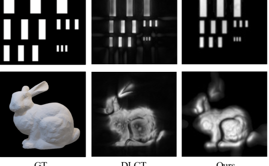
Figure 4: Reconstruction results on the confocally scanned $256\times 256$ transients of USAF and Bunny with a planar relay wall.

	LCT	FK	Phasor	DLCT	Ours
MAE	0.1706	0.0876	0.1113	0.3065	0.0542
RMSE	0.2667	0.2040	0.2611	0.4103	0.1629

Table 1: Quantitative results of the depth maps on ZNLOS Bunny.

Results on sparsely scanned transients. To evaluate the results on the sparsely scanned transients, experiments are conducted on $32\times 32$ transients, obtained by taking the subset of the original measurements with appropriate strides. We report the results on USAF and Bunny in ZNLOS [6], and Statue and Dragon in the real-world dataset [14].

The qualitative results are reported in Figure 3. The results of DLCT contain pale artifacts around the hidden objects, making some objects indistinguishable from these artifacts. The overall shapes of the objects are well reconstructed in the outputs of FK [14] and Phasor field [18], they often fail to reveal fine details of the objects, e.g. the ear of Bunny and the head of Dragon. On the other hand, our method shows superior performance compared to other method, by successfully recovering clean and sharp results with fine details on both synthetic and real-world transients.

We also quantitatively evaluate the results of depth maps on $32\times 32$ transients of Bunny. Since the ground truth was provided at a resolution of $256\times 256$, we compare the results by upsampling the low-resolution results with trilinear interpolation. For fair comparisons, we also utilize the 5% thresholding technique similar to our method to report the baseline results, due to the presence of the artifacts in them. The depth maps are evaluated using the mean absolute error (MAE) and root mean squared error (RMSE), which are computed based on the maximum values for each z-axis. As can be seen in Table 1, our proposed method achieves the best results in both metrics, showing that our method reconstructs the accurate geometry as well as the visual appearance.

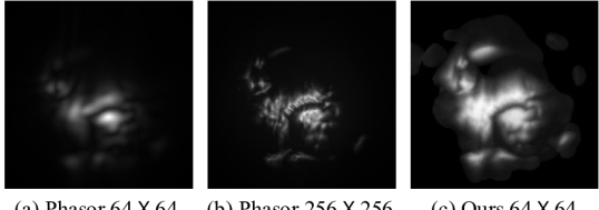
Figure 5: Results on ZNLOS Bunny under the non-confocal setup.

Results on high-resolution transients. To clearly validate the quality of our method, we report the qualitative results on commonly used $256\times 256$ high-resolution transients of Bunny. We compare our results with DLCT [31], which shares most similar image formation model with our method. As illustrated in Figure 4, our approach is able to recover the clean results on USAF and Bunny, achieving comparable results with DLCT. Although DLCT produces favorable results overall, it can be observed that DLCT lacks some fine details, e.g. in the body of Bunny.

4.2 Evaluation in various scenarios

We present the versatility and the extensiblity to several real-world scenarios through the experiments conducted in various scenarios. We report the results on the transients obtained with non-confocal scanning and non-planar relay wall, and the results of surface reconstruction.

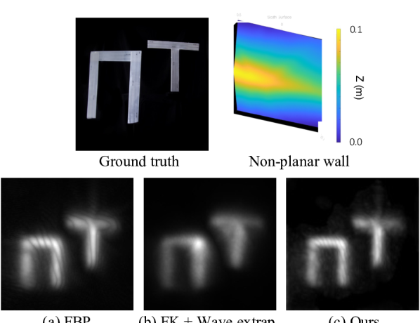
Figure 6: Results on the real-world $128\times 128$ transients [14], measured with a non-planar relay wall.

Non-confocal system. We present our results on non-confocally measured $64\times 64$ transients of Bunny. The results of Phasor field [18] on the transients acquired using both $64\times 64$ and $256\times 256$ scan points are compared. We illustrate the qualitative results in Figure 5. Phasor field fails to recover some details in the case of sparsely scanned transients, resulting the coarse and blurry outputs. In the case of high-resolution transients, Phasor field reveals more details than using the $64\times 64$ transients, but still misses some details and produces visible distortions in the outputs. Unlike these results, our method successfully recovers cleaner results with more fine details even using the $64\times 64$ measurements, which support superiority of our method.

Non-planar relay wall. We conduct the experiments on the real-world transients measured with a non-planar wall [14], to show that our method can be applied to arbitrary types of the sampling geometry. The formulation of our light propagation model is slightly adjusted in this experiment to properly deal with the retro-reflective targets. We compare the results with FBP [29] and FK [14]. The additional wave extrapolation technique is applied to report the results of FK, as the relay wall is assumed to be a planar wall in its algorithm. Figure 6 demonstrates the results of non-planar relay wall setup. FBP is effective at reconstructing the silhouette, but its results tend to be blurry and show some distortions. FK [14] recovers the blurry shapes of the objects with the incorrect albedo values at some regions such as the shape of T. Our method reconstructs the clean shapes of the objects with more correct albedo values, showing the extensibility of our method beyond the planar relay wall.

Surface reconstruction. Our method is capable of reconstructing the surfaces of the hidden objects, as our method reconstructs the surface normal as well as the albedo. To report the surface reconstruction results, we apply the threshold in a similar to the way used in DLCT [31] and apply Poisson reconstruction [11]. As illustrated in Figure 3, our method is able to accurately recover the surface geometry, as well as the visual appearance of the objects. The surface reconstruction results of our method also includes the results on non-confocal measurements of Bunny, showcasing the versatility of our method.

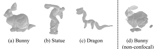
Figure 7: Surface reconstruction results. Results on confocal $32\times 32$ transients of (a) Bunny, (b) Statue and (c) Dragon. (d) Results on non-confocal $64\times 64$ transients of Bunny.

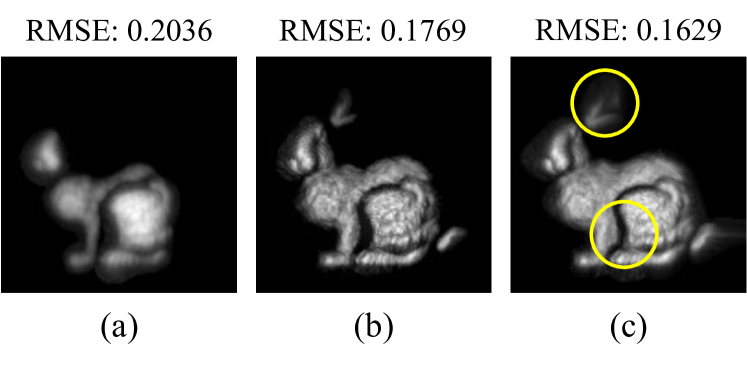
Figure 8: Ablation results on the radiometric fall-off terms. (a) Result without both distance and cosine fall-off. (b) Result without cosine fall-off. (c) Result with both distance and cosine fall-off. The above MSE measures the quality of depth map reconstruction. The model with both fall-off terms (c) achieves the best result both qualitatively and quantitatively.

5 Analysis and ablation study

In this section, we provide deeper insights and analysis of our proposed concepts. We first illustrate the effects of fall-off modeling in our light modeling through the ablation. Then we provide the analysis of reconstruction time to examine the efficiency improvement of our domain reduction.

Ablation on fall-off modeling. We conduct the ablation study of both cosine and distance based radiometric fall-off to show how the accurate light modeling affects to the reconstruction quality. The results on ZNLOS Bunny obtained with $32\times 32$ confocal scanning and a planar relay wall are reported. We compare the results of three variants of our method: (a) optimized without both cosine and distance fall-off terms, (b) model that uses distance fall-off but assumes isotropic scatter (no cosine fall-off), and finally (c) model with all fall-off terms. As reported in Figure 8, our method with both fall-off terms shows the best results, while the other results miss several details. The model without both terms (a) shows the worst result, only recovering the silhouette of the bunny. The model only without cosine fall-off (b) reconstructs almost all details, but still fails to recover some parts in details (circled parts in Figure 8). These results support that the accurate modeling of light propagation leads to the significant improvement of quality.

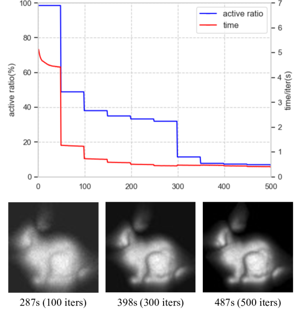
Figure 9: The active ratio and timer per iteration during the optimization, with the output resolution $64\times 64\times 666$.

Analysis of reconstruction time. Similar to previous optimization-based methods, the time complexity of our method in the initial phase requires $(N^{3}M^{2})$ per iteration, where $N$ denotes the grid resolution of the hidden space and $M$ denotes the resolution of scan points. However, thanks to the powerful ability of our domain reduction strategy, such massive computations only occur in the early steps and are drastically reduced as the empty regions are pruned.

In Figure 9, we report the time per iteration and the ratio of active areas during the optimization. The ratio of active areas rapidly decreases and reaches lower than 40% at 100th step, where we can already reconstruct the overall shape of the bunny. After 500 iterations, our domain is reduced to less than 7% of the entire space (6.68%), leading to approximately a 15$\times$ acceleration of our optimization process. With further enhancement brought by our coarse-to-fine strategy at the initial phase, our method is able to reconstruct the hidden volumes in a much efficient way.

Runtime comparison. Such efficiency gains can also be seen in the comparisons of reconstruction time with [22]. The overall optimization scheme of [22] is most similar to our method among the optimization-based methods, but our method is able to reconstruct the hidden scenes much efficiently, thanks to our domain reduction strategy. We measure the optimization time of our method under the same environment setup: $32\times 32$ transients, same number of depth planes, using a single RTX 2080Ti GPU, and total 2000 iterations. Since [22] reports the reconstruction time for $16\times 16$ outputs, we first report the reconstruction time for $16\times 16$ output resolution, and then we gradually increase our output resolution to examine the effects of the domain reduction.

As shown in Table 2, our method achieves almost a $1.62\times$ speedup with the same $16\times 16$ output resolution. Although the number of total grid bins of the output volumes is increased by $4\times$, the reconstruction time of our method for $32\times 32$ outputs is almost similar to [22] for $16\times 16$ outputs, requiring only about 10% more time. The efficiency gain from our domain reduction becomes greater as the output resolution increases. This can be observed when we increase our output resolution to $64\times 64$, where the reconstruction time is only increased by $1.29\times$ while the computations are increased to $4\times$, exhibiting the efficiency of our domain reduction especially for the high-resolution outputs.

	Dynamic [22]	Ours
Resolution	$16\times 16$	$16\times 16$	$32\times 32$	$64\times 64$
Time (s)	20.00	12.27	22.18	28.57

Table 2: Reconstruction time comparison. The time of [22] is reported in their paper with $z$-axis resolution 64, and the time of our method is reported with $z$-axis resolution 66.

6 Discussion and conclusion

This paper presented the new optimization-based method that can solve the NLOS imaging problem under the various NLOS scenarios. We showed that our method, which decomposes transients to a linear combination of 3D sub-signals, has broad applicability in many NLOS cases, including confocal, non-confocal, non-planar relay wall and the sparse scanning. The memory complexity of our method is O($N^{3}$), enabling the hidden scenes to be reconstructed by our method using a single commercial GPU.

While we achieved high-quality results under various setups, the concerns about noise have not been fully discovered in this paper. Although our proposed method showed the ability to reconstruct the hidden scenes with noise [14] (real-world scenes), we expect that such noise can be more effectively addressed. Moreover, the reconstruction of the hidden scenes with self-occlusion is worth exploring subject, which we plan to resolve in our future research.

References

- [1] Byeongjoo Ahn, Akshat Dave, Ashok Veeraraghavan, Ioannis Gkioulekas, and Aswin C Sankaranarayanan. Convolutional approximations to the general non-line-of-sight imaging operator. In Proceedings of the IEEE/CVF International Conference on Computer Vision (ICCV), pages 7889–7899, 2019.
- [2] Victor Arellano, Diego Gutierrez, and Adrian Jarabo. Fast back-projection for non-line of sight reconstruction. Optics express, 25(10):11574–11583, 2017.
- [3] Mufeed Batarseh, Sergey Sukhov, Zhiqin Shen, Heath Gemar, Reza Rezvani, and Aristide Dogariu. Passive sensing around the corner using spatial coherence. Nature communications, 9(1):1–6, 2018.
- [4] Jeremy Boger-Lombard and Ori Katz. Passive optical time-of-flight for non line-of-sight localization. Nature communications, 10(1):1–9, 2019.
- [5] Javier Grau Chopite, Matthias B Hullin, Michael Wand, and Julian Iseringhausen. Deep non-line-of-sight reconstruction. In Proceedings of the IEEE/CVF Conference on Computer Vision and Pattern Recognition (CVPR), pages 960–969, 2020.
- [6] Miguel Galindo, Julio Marco, Matthew O’Toole, Gordon Wetzstein, Diego Gutierrez, and Adrian Jarabo. A dataset for benchmarking time-resolved non-line-of-sight imaging, 2019.
- [7] Javier Grau, Markus Plack, Patrick Haehn, Michael Weinmann, and Matthias Hullin. Occlusion fields: An implicit representation for non-line-of-sight surface reconstruction. arXiv preprint arXiv:2203.08657, 2022.
- [8] Felix Heide, Matthew O’Toole, Kai Zang, David B Lindell, Steven Diamond, and Gordon Wetzstein. Non-line-of-sight imaging with partial occluders and surface normals. ACM Transactions on Graphics (TOG), 38(3):1–10, 2019.
- [9] Mariko Isogawa, Dorian Chan, Ye Yuan, Kris Kitani, and Matthew O’Toole. Efficient non-line-of-sight imaging from transient sinograms. In Proceedings of the European Conference on Computer Vision (ECCV), pages 193–208. Springer, 2020.
- [10] Mariko Isogawa, Ye Yuan, Matthew O’Toole, and Kris M Kitani. Optical non-line-of-sight physics-based 3d human pose estimation. In Proceedings of the IEEE/CVF Conference on Computer Vision and Pattern Recognition (CVPR), pages 7013–7022, 2020.
- [11] Michael Kazhdan, Matthew Bolitho, and Hugues Hoppe. Poisson surface reconstruction. In Proceedings of the fourth Eurographics symposium on Geometry processing, volume 7, 2006.
- [12] Diederik P Kingma and Jimmy Ba. Adam: A method for stochastic optimization. arXiv preprint arXiv:1412.6980, 2014.
- [13] Ahmed Kirmani, Tyler Hutchison, James Davis, and Ramesh Raskar. Looking around the corner using transient imaging. In Proceedings of the IEEE/CVF International Conference on Computer Vision (ICCV), pages 159–166. IEEE, 2009.
- [14] David B Lindell, Gordon Wetzstein, and Matthew O’Toole. Wave-based non-line-of-sight imaging using fast fk migration. ACM Transactions on Graphics (TOG), 38(4):1–13, 2019.
- [15] Lingjie Liu, Jiatao Gu, Kyaw Zaw Lin, Tat-Seng Chua, and Christian Theobalt. Neural sparse voxel fields. NeurIPS, 2020.
- [16] Xiaochun Liu, Sebastian Bauer, and Andreas Velten. Analysis of feature visibility in non-line-of-sight measurements. In Proceedings of the IEEE/CVF Conference on Computer Vision and Pattern Recognition (CVPR), pages 10140–10148, 2019.
- [17] Xiaochun Liu, Sebastian Bauer, and Andreas Velten. Phasor field diffraction based reconstruction for fast non-line-of-sight imaging systems. Nature communications, 11(1):1–13, 2020.
- [18] Xiaochun Liu, Ibón Guillén, Marco La Manna, Ji Hyun Nam, Syed Azer Reza, Toan Huu Le, Adrian Jarabo, Diego Gutierrez, and Andreas Velten. Non-line-of-sight imaging using phasor-field virtual wave optics. Nature, 572(7771):620–623, 2019.
- [19] Ricardo Martin-Brualla, Noha Radwan, Mehdi SM Sajjadi, Jonathan T Barron, Alexey Dosovitskiy, and Daniel Duckworth. Nerf in the wild: Neural radiance fields for unconstrained photo collections. In Proceedings of the IEEE/CVF Conference on Computer Vision and Pattern Recognition (CVPR), pages 7210–7219, 2021.
- [20] Ben Mildenhall, Pratul P Srinivasan, Matthew Tancik, Jonathan T Barron, Ravi Ramamoorthi, and Ren Ng. Nerf: Representing scenes as neural radiance fields for view synthesis. In Proceedings of the European Conference on Computer Vision (ECCV), pages 405–421. Springer, 2020.
- [21] Matthew O’Toole, David B Lindell, and Gordon Wetzstein. Confocal non-line-of-sight imaging based on the light-cone transform. Nature, 555(7696):338–341, 2018.
- [22] Chengquan Pei, Anke Zhang, Yue Deng, Feihu Xu, Jiamin Wu, U David, Lei Li, Hui Qiao, Lu Fang, and Qionghai Dai. Dynamic non-line-of-sight imaging system based on the optimization of point spread functions. Optics Express, 29(20):32349–32364, 2021.
- [23] Charles Saunders, John Murray-Bruce, and Vivek K Goyal. Computational periscopy with an ordinary digital camera. Nature, 565(7740):472–475, 2019.
- [24] Sheila W Seidel, John Murray-Bruce, Yanting Ma, Christopher Yu, William T Freeman, and Vivek K Goyal. Two-dimensional non-line-of-sight scene estimation from a single edge occluder. IEEE Transactions on Computational Imaging, 7:58–72, 2020.
- [25] Siyuan Shen, Zi Wang, Ping Liu, Zhengqing Pan, Ruiqian Li, Tian Gao, Shiying Li, and Jingyi Yu. Non-line-of-sight imaging via neural transient fields. IEEE Transactions on Pattern Analysis and Machine Intelligence (PAMI), 43(7):2257–2268, 2021.
- [26] Kenichiro Tanaka, Yasuhiro Mukaigawa, and Achuta Kadambi. Polarized non-line-of-sight imaging. In Proceedings of the IEEE/CVF Conference on Computer Vision and Pattern Recognition (CVPR), pages 2136–2145, 2020.
- [27] Chia-Yin Tsai, Kiriakos N Kutulakos, Srinivasa G Narasimhan, and Aswin C Sankaranarayanan. The geometry of first-returning photons for non-line-of-sight imaging. In Proceedings of the IEEE/CVF Conference on Computer Vision and Pattern Recognition (CVPR), pages 7216–7224, 2017.
- [28] Chia-Yin Tsai, Aswin C Sankaranarayanan, and Ioannis Gkioulekas. Beyond volumetric albedo–a surface optimization framework for non-line-of-sight imaging. In Proceedings of the IEEE/CVF Conference on Computer Vision and Pattern Recognition (CVPR), pages 1545–1555, 2019.
- [29] Andreas Velten, Thomas Willwacher, Otkrist Gupta, Ashok Veeraraghavan, Moungi G Bawendi, and Ramesh Raskar. Recovering three-dimensional shape around a corner using ultrafast time-of-flight imaging. Nature communications, 3(1):1–8, 2012.
- [30] Adam B Yedidia, Manel Baradad, Christos Thrampoulidis, William T Freeman, and Gregory W Wornell. Using unknown occluders to recover hidden scenes. In Proceedings of the IEEE/CVF Conference on Computer Vision and Pattern Recognition (CVPR), pages 12231–12239, 2019.
- [31] Sean I Young, David B Lindell, Bernd Girod, David Taubman, and Gordon Wetzstein. Non-line-of-sight surface reconstruction using the directional light-cone transform. In Proceedings of the IEEE/CVF Conference on Computer Vision and Pattern Recognition (CVPR), pages 1407–1416, 2020.
- [32] Alex Yu, Ruilong Li, Matthew Tancik, Hao Li, Ren Ng, and Angjoo Kanazawa. Plenoctrees for real-time rendering of neural radiance fields. In Proceedings of the IEEE/CVF International Conference on Computer Vision, pages 5752–5761, 2021.