Monitoring a developing pandemic with available data

Abstract

This paper addresses pandemic statistics from a management perspective. Both input and output are easy to understand. Focus is on operations and cross border communication. To be able to work with simple available data some new missing data issues have to be solved from a mathematical statistical point of view. We illustrate our approach with data from France collected during the recent Covid-19 pandemic. Our new benchmark method also introduces a potential new division of labour while working with pandemic statistics allowing crucial input to be fed to the model via prior knowledge from external experts.

Keywords:Local linear estimation; Missing data; Forecasting; Management; Pandemic

1 Introduction

Let $N_{1}$, $N_{2}$, $N_{3}$ and $N_{4}$ be four time series counting daily positive tests for the infection ($N_{1}$), entrances into hospital ($N_{2}$), released alive from hospital ($N_{3}$) and dead at hospital ($N_{4}$). Let $F$ be a fifth time series measuring the relative number of pandemic patients dying in hospital versus the number of patients dying outside hospital.

To model and forecast the development of these five stochastic processes would provide us with a good benchmark model when monitoring a developing pandemic. The advantage of this approach is that the four counting processes have shown to be readily available in many countries and regions of countries from the early days of a pandemic. We could even follow the numbers in many daily newspapers when the Covid-19 pandemic was at its height. The fifth stochastic process $F$ is also available: death is most often recorded well. The challenge of this approach is that understanding the statistical properties of the important counting process transitions (between $N_{1}$ and $N_{2}$ for example) is not easy. There is a missing link problem arising from the fact that we do not have records of the exact individuals and their exact infection time resulting in exactly when these individuals get infected or enter or leave hospital. We have only the above simple four counting processes and their aggregated information. This missing link estimation problem has been investigated to some extent in probabilistic queueing theory see for example Goldenshluger and Koops (2019), but not to the level of direct practicality that we need to develop a practical approach to monitoring a pandemic. One difficulty we face while modelling a pandemic that (to our knowledge) has not been considered in queuing theory is that $N_{1}(t)$ is not the number of individuals getting infected at day $t$, it is something much more tricky, it is the number of individuals tested positive at day $t$. Missing link survival analysis was introduced in Gámiz, Mammen, Martínez-Miranda and Nielsen (2022, 2023), where the latter of these two papers introduced the concept of “exposure of low quality” for the changing nature of the exposure information given by $N_{1}$ when trying to forecast future values of $N_{1}$ and $N_{2}$. We will now shortly review related recent literature on monitoring a developing pandemic.

In the beginning of a pandemic policy makers and other decision makers face the challenge of having to take important decision based on limited data, see Britton and Tomba (2019). While the outbreak of the pandemic might have a global nature, local decisions have to be taken fast, see Chang and Kaplan (2023). Understanding the dynamic of a pandemic is important for decisions and policy making in general, see Dillon et al. (2023) and Garrett (2023). Specific applications could for example be vaccine prioritization and planning, see Lee et al. (2015), Follmann and Fay (2021), Thul and Powell (2023) or food planning, see Ekici et al. (2014), the labour market, see Cao et al. (2022), teaching and learning, see Ko et al. (2023), portfolio choice, see Kraft and Weiss (2023), hospital occupancy and mortality, see Gutiérrez and Rubli (2021), older adult care, see Kong et al. (2021) and various resource optimization challenges during a pandemic, see Rautenstrauss et al. (2023), Yin et al. (2023), Hammami et al. (2023). This quick review of operational research and biostatistical studies on concrete application of pandemic modelling shows that it could be valuable to have some benchmark pandemic modelling that is based on available data that is quickly understood across national and regional boundaries. This was also pointed out in recent methodological discussions recommending improved communication between countries and local communities when quick decisions have to be taken, see Mukherjee (2022), Lin (2022) and Gao et al. (2020). It is not that we do not have methodology to estimate the development of a pandemic, see for example Farahani et al. (2023), Lu and Borgonovo (2023), Das et al. (2023), Slater et al. (2023), Mahsin et al. (2022), Sparapani et al. (2020), Mukherjee and Seshadri (2022) and Quick et al. (2021) among many others, but none of these provides a simple benchmark method only using the available easy to communicate counting processes $N_{1}$, $N_{2}$, $N_{3}$, $N_{4}$ and $F$. So, the purpose of this paper is to introduce a simple benchmark method that is easy to implement with the data at hand; data that is available and understood across international and national borders. Based on our experience with the recent Covid-19 pandemic, we expect $N_{1}$, $N_{2}$, $N_{3}$, $N_{4}$ and $F$ to be available, perhaps with some prior knowledge on the so called reproduction number and the relationship between deaths inside and outside hospitals at given points in time. Our approach can be extended by prior knowledge and expert opinion that is often developed in the beginning and throughout a pandemic. In the Covid-19 pandemic the reproduction number (the $R$-number) was omnipresent while discussing the development of the pandemic and was even broadcasted on the news or published in daily newspapers. Our method is able to take such information (as the $R$-number) and incorporate it into the pandemic modelling as prior knowledge or expert opinion. Our methodology also allow for prior knowledge or expert opinion to be included when forecasting how many die inside hospitals compared to how many that die outside hospitals (for example in care homes). It is of course also fully aligned with our approach to fit the $R$-number via a regression methodology as suggested in Quick et al. (2021). The communication of our method is easy, because both input and output are easy to understand, and our method is not depending on underlying assumptions that are difficult to communicate.

We simplify scientific cooperation: the scientists or practitioners providing the single number of prior knowledge used when forecasting (such as experts on the $R$-number) do not need to be experts in the general scientific modelling of the rest of the problem.

The organisation of the paper is as follows:

Section 2 introduces new methodology on dynamic missing link survival analysis based on multivariate marker dependent hazard estimation. This is essential for duration analysis of hospital stays. In Section 3 it is illustrated how the methodology of Section 2 can be combined with the infection to infection and infection to hospital analysis of Gámiz et al. (2023) to provide a full system from infection to leaving hospital. In Section 4 the concrete case of the recent Covid-19 pandemic in France is analysed. It is also shown how mortality outside hospitals can be incorporated in the analysis and it is shown how prior knowledge on the reproduction number, the $R$-number, and prior knowledge on the current ratio of deaths inside versus outside hospitals can be incorporated into the analysis. In Section 5 a finite sample simulation study is provided that shows that our new methodology is overcoming the new missing link survival analysis challenges well. Section 6 provides the conclusions of the paper.

2 Modelling time to outcome durations

We concentrate in this section on generalising the missing link survival analysis of Gámiz et al. (2022) to the dynamic and multivariate situation needed to investigate the transitions from $N_{2}$ to $N_{3}$ and from $N_{2}$ to $N_{4}$. The transitions from $N_{1}$ to $N_{1}$ and from $N_{1}$ to $N_{2}$ were treated inGámiz et al. (2023) via Hawkes processes (Mammen and Müller (2023)) where a new definition of “exposure of low quality” is used. In Section 3 we incorporate the stochastic process $F$ in our analyses to complete a full methodology for “monitoring a developing pandemic with available data”.

In this section, we first describe a model for the hazard function of the survival time when the outcome is death or hospital discharge. Then we propose a new estimator that works in the hypothetical situation where we have full information of the follow up of each individual and where we therefore do not face the missing link problem in survival analyses. We will refer to this situation with the term “full information”.

Finally, we present an algorithm able to generate information of the time-from-hospitalization-to-leaving-the-hospital from available data where the missing link survival problem has to be solved

2.1 Model formulation

Using the notation of Section 1, let $N_{2}(t)$ count the number of persons hospitalized in the interval $(0,t]$ for $0<t\leq T$. Note that $N_{2}(t)=\sum_{i=1}^{k}\left(N_{2}(t\cdot i/k)-N_{2}(t\cdot(i-1)/k)\right)$ for $k$ large enough, which following usual notation in counting process theory we also write as $N_{2}(t)=\int_{0}^{t}N_{2}(du)$, where $N_{2}(du)$ can be interpreted as the number of new hospitalized in the interval $(t,t+{\mathrm{d}}t]$.

The hospitalized persons can leave the hospital due to death or recovery, whichever occurs first. Let us denote $N_{\cdot}(t)$ the total number of patients that leave hospital in $(0,t]$, then $N_{\cdot}(t)=N_{3}(t)+N_{4}(t)$, where as in Section 1 $N_{3}(t)$ counts the number of patients that receive medical discharge and $N_{4}(t)$ the number of patients that die in hospital in the interval $(0,t]$. Then $N_{\cdot}({\mathrm{d}}t)$ is the number of persons that leave the hospital (due to death or recovery) in the interval $(t,t+{\mathrm{d}}t]$, and $N_{\cdot}(t)=\int_{0}^{t}N_{\cdot}({\mathrm{d}}s)$, for $0<t\leq T$. Furthermore, we write $N_{\cdot}({\mathrm{d}}t,{\mathrm{d}}s)$ for the number of persons who entered the hospital in $(s,s+{\mathrm{d}}s]$ and leave in $(t,t+{\mathrm{d}}t]$ due to any cause, $s<t\leq T$.

Let $\lambda$ denote the intensity function of $N_{\cdot}$, that is,

$$\lambda(t)=\lim_{{\mathrm{d}}t\rightarrow 0}\frac{P(N_{\cdot}(t+{\mathrm{d}}t)-N_{\cdot}(t)\geq 1\mid{\cal F}(t))}{{\mathrm{d}}t},\ 0<t\leq T,$$

where ${\cal F}(t)$ is the $\sigma$-field generated by $\{(N_{2}(s),N_{\cdot}(s)):s<t\}$.

We assume that

$$\lambda(t)=\int_{0}^{t-}\mu(t,t-s)Y(t,s)N_{2}({\mathrm{d}}s),$$ (1)

where $\mu(t,t-s)$ is the hazard function for the duration time in the hospital for an individual that entered at time $s$ and leaves at time $t$, and $Y(t,s)$ counts the number of individuals still remaining in hospital at time $t$ among those who entered at time $s$, with $s<t$.

We observe $n$ individuals in the interval $(0,T]$, where we denote $N_{\cdot,i}(t)$ the process that counts 1 if individual $i$ has left the hospital (due to death or recovery) in $(0,t]$ and 0 otherwise, and denote its intensity function $\lambda_{i}(t)$, for $i=1,\ldots,n$. Let us assume for instance that $0<S_{1}<\ldots<S_{n}<T$ are $n$ distinct hospitalization times, then, from (1),

$$\lambda(t)=\sum_{i=1}^{n}\mu(t,t-S_{i})Y_{i}(t),$$

where we denote $Y_{i}(t)=Y(t,S_{i})\ I(S_{i}<t)$, for $i=1,\ldots,n$.

We have that $N_{\cdot}(t)=\sum_{i=1}^{n}N_{\cdot,i}(t)$, and also $\lambda(t)=\sum_{i=1}^{n}\lambda_{i}(t)$, so $\lambda_{i}(t)=\mu(t,t-S_{i})Y_{i}(t)$ fits the multiplicative Aalen’s model (see Nielsen (1998) for a more general description of the model).

Our aim is to estimate $\mu(t,t-s)$, for $0<s<t\leq T$. To do it we need observations of the process $N_{\cdot}(t,{\mathrm{d}}s)=\sum_{i=1}^{n}N_{\cdot,i}(t,{\mathrm{d}}s)$, where $N_{\cdot,i}(t,{\mathrm{d}}s)$ takes value 1 if the individual $i$, hospitalized in $(s,s+{\mathrm{d}}s]$, leaves at some time in the interval $(s,t]$. Ideally we observe these processes but in our motivating application we only observe the marginal processes $N_{2}(t)$ and $N_{\cdot}(t)$. In the next section, we address the estimation of $\mu$ in the ideal case of full information and afterwards we will describe our algorithm for estimating $\mu$ with available data.

2.2 Estimator of the two-dimensional hazard when full information is available

With full information we observe $(N_{2,1}({\mathrm{d}}s),N_{\cdot,1}(t,{\mathrm{d}}s)),\ldots,(N_{2,n}({\mathrm{d}}s),N_{\cdot,n}(t,{\mathrm{d}}s))$ independent and identically distributed couples of processes, $s<t\leq T$.

We are interested in estimating the two-dimensional intensity $\mu(t,t-s)$ with no restriction on its functional form.

Then the local-linear estimator of $\mu$ can be written

$$\widehat{\mu}(t,t-s)$$ (2)

$$=\frac{\int_{0\leq v<u\leq T}{\rm C}(s,t,u,v)\ K_{1,b_{1}}\left(t-u\right)K_{2,b_{2}}(t-s-(u-v))N_{\cdot}({\mathrm{d}}u,{\mathrm{d}}v)}{\int_{0\leq v<u\leq T}{\rm C}(s,t,u,v)\ K_{1,b_{1}}\left(t-u\right)K_{2,b_{2}}(t-s-(u-v))Y(u,v){\mathrm{d}}v{\mathrm{d}}u}$$

for $0\leq v<u\leq T$, and with $N_{\cdot}({\mathrm{d}}u,{\mathrm{d}}v)$ and $Y(u,v)$ defined previously.

Notice that the estimator is a ratio of a local linear estimator of occurrences and a local linear estimator of exposure, see Nielsen (1998) that is a local linear generalisation of Nielsen and Linton (1995).

In (2) we have used the following notation: For $j=1,2$, $K_{j,b_{j}}(\cdot)=K_{j}(\cdot/b_{j})/b_{j}$, where $K_{j}$ is a general one-dimensional kernel function. We denote

$${\rm C}(s,t,v,u)=1-\big{(}t-u,t-s-(u-v)\big{)}^{t}{\rm{\bf A}}(t,s)^{-1}{\rm{\bf a}}(t,s)$$ (3)

for $0\leq s<t\leq T$. Here ${\rm{\bf a}}$ be a vector function whose $l$th component is

$${\rm a}_{l}(t,s)=\int_{0\leq v<u\leq T}K_{1,b_{1}}\left(t-u\right)K_{2,b_{2}}(t-s-(u-v))$$

$$\times\left(t-u\right)^{\delta_{l1}}(t-s-(u-v))^{\delta_{l2}}Y(u,v){\mathrm{d}}v{\mathrm{d}}u$$ (4)

for $l=1,2$; being $\delta_{lh}=1$ if $l=h$, and 0, otherwise. Also, ${\rm{\bf A}}$ is a matrix function with dimension $2\times 2$ whose $(l,m)$-element is given by

$${\rm A}_{l,m}(t,s)=\int_{0\leq v<u\leq T}K_{1,b_{1}}\left(t-u\right)K_{2,b_{2}}(t-s-(u-v))$$

$$\times\left(t-u\right)^{\delta_{l1}+\delta_{m1}}(t-s-(u-v))^{\delta_{l2}+\delta_{m2}}Y(u,v){\mathrm{d}}v{\mathrm{d}}u,$$ (5)

for $l,m=1,2$, with $\delta_{h}$ defined above, and $\delta_{mh}=1$ if $m=h$ and 0 otherwise.

We denote $\mu_{3}(t,t-s)$ the recovery hazard function at time $t$ for a subject that entered the hospital at time $s$, and $\mu_{4}(t,t-s)$ the mortality hazard function at time $t$ for a subject that entered the hospital at time $s$. We can use the same formulation as in (2) to build two-dimensional local-linear estimators $\widehat{\mu}_{3}$, and $\widehat{\mu}_{4}$, respectively.

2.3 An iterative estimation scheme approximating the infeasible estimator of the hazard

In the case that full information is not available, this is, we observe only the marginal processes $N_{2}(t)$ and $N_{\cdot}(t)$, we describe an iterative estimation scheme for the estimation of $\mu$.

At the $r$th iteration of the algorithm we have an estimated value of $\mu$ from the last iteration that we denote by $\widehat{\mu}^{(r-1)}$. For $r=1$ we use an initial guess $\widehat{\mu}^{(0)}$ of $\mu$. The $r$th iteration of the algorithm consists of two steps:

1. In the first step, we construct a two-dimensional process $\hat{N}^{(r)}(t,{\mathrm{d}}s)$ that approximates $N(t,{\mathrm{d}}s)$ and a two-dimensional process $\hat{Y}^{(r)}(t,s)$ that approximates $Y(t,s)$. This is done by using the estimator $\widehat{\mu}^{(r-1)}$ from the previous iteration and by using the observed processes $N_{2}(t)$ and $N(t)$. Let us denote

   $$\widehat{S}^{(r)}(t,t-s)=\prod\limits_{s<u\leq t}\!\left\{1-\widehat{\mu}^{(r)}(u,u-s){\mathrm{d}}u\right\}.$$

   the estimated probability that a subject hospitalized at time $s$ still remains in hospital at time $t$. Similarly to Gámiz et al. (2023), we define

   $$\hat{N}^{(r)}({\mathrm{d}}u,{\mathrm{d}}v)=\frac{\widehat{S}^{(r)}(u,u-v)\widehat{\mu}^{(r)}(u,u-v)N_{2}({\mathrm{d}}v)}{\displaystyle{\int_{0}^{u-}}\!\widehat{S}^{(r)}(u,u-w)\widehat{\mu}^{(r)}(u,u-w)N_{2}({\mathrm{d}}w)}N_{\cdot}({\mathrm{d}}u).$$ (6)

   and

   $$\hat{Y}^{(r)}(u,v)=\frac{\widehat{S}^{(r)}(u,u-v)N_{2}({\mathrm{d}}v)}{{\displaystyle{\int_{0}^{u-}}}\!\widehat{S}^{(r)}(u,u-w)N_{2}({\mathrm{d}}w)}Y(u),$$ (7)

   with $Y(u)=N_{2}(u)-N_{\cdot}(u)$, is the number of individuals remaining in hospital at time $u$.

2. In the second step, the estimator of $N_{\cdot}({\mathrm{d}}u,{\mathrm{d}}v)$ given in (6) and the estimator of $Y(u,v)$ given in (7) are plugged into (2). This results in the following update of $\widehat{\mu}^{(r)}$:

   $$\widehat{\mu}^{(r+1)}(t,t-s)$$ (8)

   $$\quad=\frac{\int_{0\leq v<u\leq T}{\rm C}(s,t,v,u)\ K_{1,b_{1}}\left(t-u\right)K_{2,b_{2}}(t-s-(u-v))\hat{N}_{\cdot}^{(r)}({\mathrm{d}}u,{\mathrm{d}}v)}{\int_{0\leq v<u\leq T}{\rm C}(s,t,v,u)\ K_{1,b_{1}}\left(t-u\right)K_{2,b_{2}}(t-s-(u-v))\hat{Y}^{(r)}(u,v){\mathrm{d}}v{\mathrm{d}}u}.$$

If this iteration scheme converges it will converge against the solution $\widehat{\mu}(t,t-s)$ of the equation:

$$\widehat{\mu}(t,t-s)$$ (9)

$$=\frac{{\displaystyle{\int_{0\leq v<u\leq T}}}{\rm C}(s,t,v,u)K_{1,b_{1}}\left(t-u\right)K_{2,b_{2}}(t-s-(u-v))\times\frac{\widehat{S}(u,u-v)\widehat{\mu}(u,u-v)N_{2}({\mathrm{d}}v)N_{\cdot}({\mathrm{d}}u)}{{\int_{0}^{u-}}\!\widehat{S}(u,u-w)\widehat{\mu}(u,u-w)N_{2}({\mathrm{d}}w)}}{{\displaystyle{\int_{0\leq v<u\leq T}}}{\rm C}(s,t,v,u)K_{1,b_{1}}\left(t-u\right)K_{2,b_{2}}(t-s-(u-v))\times\frac{\widehat{S}(u,u-v)N_{2}({\mathrm{d}}v)Y(u)}{{{\int_{0}^{u-}}}\!\widehat{S}(u,u-w)N_{2}({\mathrm{d}}w)}}.$$

In the next subsection we will argue that $\widehat{\mu}(t,t-s)$ is a consistent estimator.

Finally, two types of outcome are considered. Specifically, we estimate the transition rate from-hospitalized-to-recovery, $\mu_{3}(t,w)$, and the transition rate from-hospitalized-to-death, $\mu_{4}(t,w)$ , respectively, as follows. Let $\widehat{\mu}$ be the solution of the above iterative procedure based on $\hat{N}$ and $\hat{Y}$ obtained at the last iteration. For $j=3,4$, let us define the following equation, similar to (6),

$$\hat{N}_{j}({\mathrm{d}}u,{\mathrm{d}}v)=\frac{\widehat{S}(u,u-v)\widehat{\mu}(u,u-v)}{\displaystyle{\int_{0}^{u-}}\!\widehat{S}(u,u-v)\widehat{\mu}(u,u-w)N_{2}({\mathrm{d}}w)}N_{2}({\mathrm{d}}v)N_{j}({\mathrm{d}}u).$$ (10)

then

$$\widehat{\mu}_{j}(t,t-s)$$ (11)

$$=\frac{\int_{0\leq v<u\leq T}{\rm C}(s,t,v,u)\ K_{1,b_{1}}\left(t-u\right)K_{2,b_{2}}(t-s-(u-v))\hat{N}_{j}({\mathrm{d}}u,{\mathrm{d}}v)}{\int_{0\leq v<u\leq T}{\rm C}(s,t,v,u)\ K_{1,b_{1}}\left(t-u\right)K_{2,b_{2}}(t-s-(u-v))\hat{Y}(u,v){\mathrm{d}}v{\mathrm{d}}u},$$

for $j=3,4$, respectively.

When choosing the bandwidths $b_{1}$ and $b_{2}$ for the local linear marker dependent hazard estimator above, we use the cross-validation method described in Gámiz et al. (2013) which worked well in the applications of this paper. We also tried a further development of cross-validation introduced Mammen et al. (2011), adapted to one-dimensional local linear hazards in Gámiz et al. (2016), and to marker dependent hazard estimation in Gámiz et al. (2013). This method is theoretically more robust. However, cross-validation and Do-validation gave similar results in our case and we finally decided to use the simpler cross-validation method.

We tested our new missing link marker dependent hazard estimator via finite sample simulations and found good performance where the measurement error was converging towards zero when more finite samples were included. However, the performance was (as expected) not as good as had we had we not had the missing link survival issue and had had full information from the beginning. This finite sample simulation study is deferred to Section 5.

2.4 Asymptotic analysis

It can be shown that $\widehat{\mu}(t,t-s)$ is a consistent estimator using much the same type of theoretical arguments as Gámiz et al. (2023) used in the Hawkes process case. The stochastic processes considered in this paper are counting processes and the mathematical statistics used are based on the martingale theory implied by Aalen’s multiplicative intensity model, see Nielsen (1998) and Gámiz et al. (2022) for more details. The consistency analysis of this paper can be formulated in this asymptotic framework of standard survival analyses as well with similar derivations and conclusions as in the Hawkes process case discussed in Gámiz et al. (2023). We omit the theoretical details to save space.

3 General considerations when monitoring and forecasting in a dynamic environment

Our dynamic modelling is broadly speaking based on two types of transitions. One type where the number of individuals are well defined and a follow-up type survival analysis is possible which have been discussed in Section 2. And then another type of transition where the number of individuals involved are biased by dynamic definitions and underestimation, which are fully considered in our previous work in Gámiz et al. (2023).

3.1 Modelling the dynamics of a pandemic

In this section we describe the full model chosen in the Covid-19 case of France. The dynamic model will be very dynamic indeed. Even the definition of what we observe might change as the pandemic develops. Our model can be illustrated via the stages represented in Figure 1.

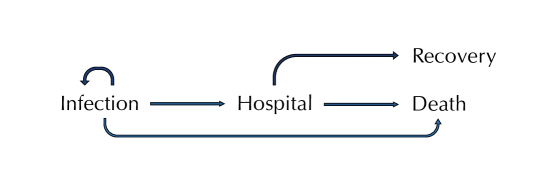
Figure 1: Transition diagram.

In a developing pandemic the first thing that happens is that a few people get infected, further infections are higher when there are many infected, therefore there is a feedback loop from the infected stage to its own stage. The definition of an infected might vary over time. A practical version would be to define infected as those people in the society that have been tested positive for the infection. In the beginning of a pandemic testing is perhaps very limited and one positive test means more than later in the pandemic when testing facilities might be widely available. Also, there might be dynamic in the transition rate from infection to hospitalization. There might be varying decisions over time (also due to seasonal impact) of when a person is hospitalized. Even definition of death might vary over time. While the definition of death itself is robust, it might vary over time what it takes to define one particular death to be due to the pandemic. Figure 1 illustrates the two possible outcome from hospital, which are respectively transitions from hospitalized to dead, and transitions from hospitalized to recovered. All transition rates in Figure 1 are modelled by two-dimensional functions, where the two dimensions are duration-in-stage and calendar-time. It is the dependency on calendar-time that provides us with the sought after dynamic.

3.2 Transitions from hospitalized to death or from hospitalized to recovered

In a confusing pandemic where definitions and measurements and other things are changed by the hour, there are stable components. It is for example often well defined what it means to be hospitalized even though the criteria for hospitalized might develop dynamically. And the daily number of hospitalized people can be expected to be recorded quite well in many countries. Death is also well defined of course even though death-by-the-pandemic can have a dynamic definition changing with a developing dynamic.

Technically speaking we cannot use standard survival analysis on the above transition when dealing with what we call “available data”. Our available data contain information of number of hospitalized every day, numbers of deaths-in-hospital every day and number of recovery-in-hospital every day. But available data does not contain information on the link between these events. We therefore do not know directly from data which hospital-durations died or recovered hospitalized had on one particular day of measurement. However, this statistical problem can be overcome by introducing some new survival techniques on missing data introduced by this paper and discussed in the methodological section.

3.3 Relationship between dying in hospital and dying outside hospital

Based on the transitions represented in Figure 1, we are now able to understand transitions from infected to infected, and from infected to hospital and from hospital to recovery or death. Even though we are only using available data. However, we are still not able to say anything about the total number of deaths in the population due to the pandemic, which are transitions from infected to death in Figure 1. To do this we need as available data the additional information on the daily number of people dying outside the hospital due the pandemic. We then operate with a dynamic ratio between number of people dying in hospital at a given date and number of people dying outside hospital at a given date, which we denote respectively $N_{\rm in}(t)$ and $N_{\rm out}(t)$. For any $t>0$, $g(t)$ is the ratio of number of deaths outside hospital over the number of deaths inside hospital, that is,

$$g(t)=\frac{N_{\rm out}(t)}{N_{\rm in}(t)}.$$

For any $t$ in the observation interval $(0,T)$ we can estimate this ratio $g(t)$ using the ratio of two non-parametric regression estimators. On the numerator, the smoothed regression on time of the number of deaths outside the hospital until $T$, and on the denominator, the smoothed regression on time of the number of deaths inside hospital until $T$. Then we estimate $\widehat{g}(t)$, for all $t\in(0,T)$.

3.4 Principles of forecasting in a dynamic environment

The main view of forecasting taken in this paper is related to the considerations of Section 3.1. We want the robust and understandable transitions to play as big a role as possible. When looking at the full system described in Section 3.1 for the Covid-19 case of France, one can take that point of view that all transitions except that one from the infection indicator to the infection indicator can be described via slowly moving continuous development over time. In other words: except for this one transition, it makes sense - at any given date - to forecast the immediate future structure of these transitions from the immediate past.

3.4.1 Forecasting the number of infections using expert knowledge.

Regarding the infection process, in Gámiz et al. (2023), we have introduced a number $C_{1,h}$ indicating whether the future, that is $(T,T+h]$ for $h>0$, will be different or equal to the immediate past. Specifically, if $C_{1,h}$ equals one then we can forecast in a time interval $(T,T+h]$ based on the immediate past.

The point of our approach to forecasting in this paper is that we could monitor and forecast the pandemic when $C_{1,h}$ equals one. In that situation a dynamic statistical methodology could do the job via a surprisingly simple data collection reflecting what can be considered “available data” in many countries. However, in a pandemic there are many change-points of severity. Therefore, the only thing left to monitor and forecast well is to have a dynamic point of view and the number $C_{1,h}$. That work needs expert advice specific to countries or local regions within countries. This important work cannot be dismissed via a statistical analysis based on simplified available data. But it is important that the experts involved should only consider forecasting and understand $C_{1,h}$ rather than being responsible for a full statistical model.

A proper value of $C_{1,h}$ at time $T$ suggested by expert knowledge makes our methodology capable of forecasting the number of new infected in $(T,T+h]$ for an $h>0$ fixed. From those, we can predict the number of hospitalized to thus forecasting of number of deaths in hospitals as well as the number of recoveries in the interval $(T,T+h]$.

3.4.2 Forecasting the total number of deaths.

In this paper we introduce another indicator $C_{2,h}$ to predict the total number of deaths, both inside and outside hospital, i.e. $N_{\rm out}+N_{\rm in}$ as defined above, based on forecasted number of infected provided by $C_{1,h}$ and the dynamic model specified in Figure 1. For any $t$ in the observation interval $(0,T]$ we consider the estimator of the ratio $g(t)$ as explained in Section 3.3. Then we have $\widehat{g}(t)$, for all $t\in(0,T]$.

Let us fix the forecast horizon at time $T+h$, for an $h>0$. We need to extrapolate the ratio $g(T+s)$, for $0<s\leq h$.

We assume that the ratio $g$ at the end of the forecasting period (i.e. $T+h$) is the more recent estimate multiplied by $C_{2,h}$, and it varies linearly in between

$$\widetilde{g}(T+s)=\widehat{g}(T)\times\left(1+(C_{2,h}-1)\frac{s}{h}\right),$$ (12)

for $0<s\leq h$.

Under the assumption that the ratio of densities is constant and equal to the most recent estimation, that is, $\widetilde{g}(T+s)=\widehat{g}(T)$, for all $0<s\leq h$, it has to be chosen $C_{2,h}=1$. On the other hand, we can consider an infeasible in practice procedure to choose the optimal value of the constant by optimizing the predicted number of daily deaths in the target forecasting interval $(T,T+h]$.

For simplicity in the following we remove the subscript $h$ from the notation and write the above indicators as $C_{1}$ and $C_{2}$.

4 Estimating with available data. The Covid-19 case of France

In this section we present our main ideas on monitoring a developing pandemic based on available data. We use the recent Covid-19 pandemic and the country France as our case study. We consider official data between 18th March 2020 and 3rd January 2022. We walk through our modelling principles and the new mathematical statistical inventions necessary to implement our new approach.

4.1 Time in hospital

It is important to construct the statistical modelling of the developing pandemic such that robust components get as much weight as possible. Time spent in hospital is such a robust component because the number of individuals involved are well defined. When analysing time spent in hospital the exact number of individuals entering and leaving hospitals are assumed to be observed every day together with the additional information on how many die at hospital every day. Notice that the collected data is aggregated in nature and individual follow-up data is not collected. We do not assume to observe which exact individuals are leaving or recovering at one particular day. This implies that standard survival methodology does not apply and we have had to introduce a new missing data methodology to the tool-box of survival analysis.

4.1.1 Examples of concrete hospital transitions, the Covid-19 case of France

Time spent in hospital is a dynamic concept in the sense that it depends on the particular date an individual is admitted to hospital. In our model $\mu(t,t-s)$, we mean by $s<t$ two different calendar times. That is, $s$ refers to the time of admission to hospital whereas $t$ is the time a patient leaves the hospital, and so, $t-s$ is the duration of hospitalization.

Figure 2 displays the estimations of the hazard function of time in hospital until recovery, $\mu_{3}$ (left panel), or death, $\mu_{4}$ (right panel), for individuals entering at different dates, that is $s$.

The plot shows curves corresponding to several values of the first dimension (a movie offering a complete dynamic view is available from the authors). For instance the solid black line in the left panel represents the hazard function of the duration until recovery for patients who enter the hospital on 30th November 2021. The hazard function can be interpreted as the probability a patient leaves the hospital due to recovery conditioned on the duration of his/her stay. The solid black line shows a decreasing tendency as time in hospital for these patients passes.

In concrete, we see that the about 6.2% of patients that entered the hospital on the 30th November 2021 received clinical discharge on the same day. Also, we can say that after a stay of 10 days, a person who was admitted to hospital on the 30th November 2021 has a probability about 0.06 of recovery, while the probability of recovery was barely of 0.037 on the 10th May 2020 for patients admitted on the 30th April 2020 (see dashed red line).

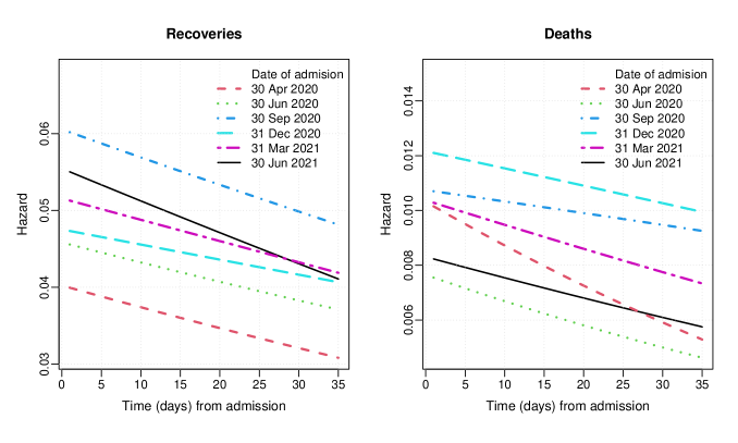
Figure 2: Hazard rate of time spent in hospital for individuals entering the hospital at different dates in the period from April 2020 to June 2021. Left panel: Hazard rate for time since admission until hospital discharge. Right panel: Hazard rate of time since admission until death.

The graph on the right panel of Figure 2 shows that for people just admitted in hospital on the 30th of April 2020 the risk of death is about 1% and decreases with the time in hospital. The risk is about 0.75% for people arriving to the hospital two months later. This can be an indicator of the collapse of the hospitals in the months immediately after the pandemic outbreak (March and April).

It should be noticed that being hospitalized or recovered, or even dying-as-infected, might be different for two different calendar times. Political decisions, available hospital resources, fatigue of hospital employees, and many other factors play a dynamic role together with the changing character of the way the pandemic itself develop in the population. Therefore, any definition in this paper is meant to be time dependent. Our mathematical formulation in this paper allows to accommodate such dynamics. The calendar time dependency of our two-dimensional marker dependent hazard is the key tool to achieve our fully flexible dynamic modelling of a developing pandemic. When it comes to our specific example of Covid-19 in France it seems evident that there is an improvement in the clinical experience and a perhaps also a better understanding of the disease from the first wave of the pandemic in the spring till the second wave of the pandemic in the fall. We can see this looking at the left panel of Figure 2. From April to September 2020, the conditional probability for a person to receive hospital discharge, given he/she has been in hospital for $x$ days, shows an increasing tendency as a function of admission date, for any value of $x$. For example, for patients just arrived ($x=1$) the probability of leaving hospital due to recovery ranges from 4% on the 30th April to 6% on the 30th September 2020.

The average daily number of new hospitalizations was around four times as high at the end of April 2020 compared to October 2020. This dynamics implied a significant pressure on hospitals in October changing the overall chances of recovering from the infection while in hospital. When studying recoveries and deaths while in hospital in Figure 2 it seems very clear that the probability of getting out of hospital alive is changing with the dynamics of the pandemic.

There are different dynamics depending on age groups. Figure 3 shows the variations in instantaneous calendar time dependent probability of death given duration in hospital (the time dependent hazard rate) for patients across different age groups.

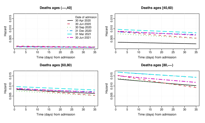
Figure 3: Hazard rate of time since admission until death for individuals entering the hospital at different dates in the period from April 2020 to November 2021.

The above described hazard rate estimators provide us with sufficient information to calculate other indicators such as the median time from admission in hospital to exit (due to recovery or death) for a given patient depending on the admission date. See Figure 4 where the median times are shown for all individuals and by age groups. A prominent peak for people hospitalized by the end of May (shown by all age groups) highlights the fact of the changing behaviour of covid on distinct times of the calendar since the pandemic outbreak. As can be seen, age is an important covariate, and, among other things, while the different conditions under which the pandemic has evolved (variants of the virus and different restrictions regimes) do not have apparently serious impact on the younger population, it seems to strongly affect people in the oldest groups for which the date of hospitalization is crucial.

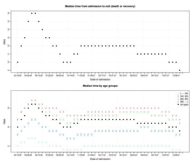
Figure 4: Median of the time spent in hospital by date of admission from March 2020 to January 2022.

Variations over time of durations of stays in hospital until recovery or death are partly explained by changes in the age of patients. In short, it can be said that the length of stays in hospital for recoveries has decreased from the first wave in about five days for the full sample. The reduction is bigger for people between 60 and 80 years and less significant for ages below 40. The length of stays for deaths has also decreased from about 17 days during the first wave until less than 12 days in the second wave, and about 10 days in the last months of 2021. This is for the full sample, the reduction being less significant for the younger patients.

Figure 5 helps to answer the following question: What is the probability that a subject who has been in hospital for $d$ days can leave it alive?

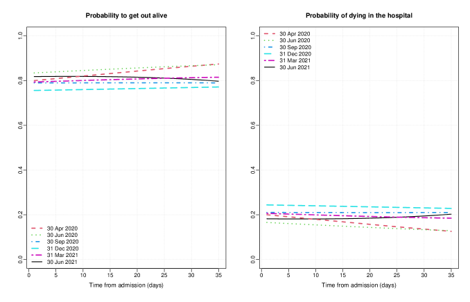
Figure 5: Probability of outcome by cause specific from March 2020 to January 2022. Left panel: Probability of leaving the hospital due to recovery. Right panel: Probability of leaving the hospital due to death.

Until September 2021 the probability of getting out alive slightly increases with the hospitalization time, specially for people above 80 years in the first month in hospital (see a graph of this probability by age groups in Figure 6). In the last months of 2021 this increase seems to revert and we can observe a decay. The probability of dying in hospital decreases with hospitalization time for admissions up to September 2021 and afterwards it increases. During the first and second wave almost 30% of the older people (above 80) will die in the first day in hospital, this percentage is about 20% for people between 60 and 80 years, and below 10% for the younger (see Figure 7). These probabilities are a bit higher in the last months of 2021 which might be explained by the effect of the vaccines and only severe cases going to hospital.

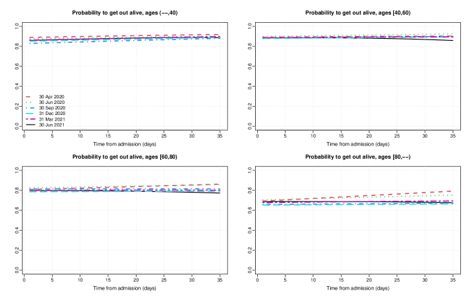
Figure 6: Probability of leaving the hospital due to recovery by age groups.

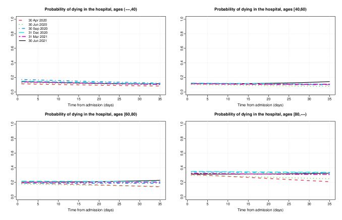
Figure 7: Probability of leaving the hospital due to death by age groups.

4.2 Examples of smooth developments of ratio of number of deaths inside versus outside hospital, the Covid-19 case of France

When quantifying the number of deaths outside hospital to be able to find the total number of deaths from the pandemic, then we simply follow the dynamic development of the ratio of people dying inside the hospital versus outside the hospital respectively, that is the function $g(t)$ defined in Section 3.3. We know from similar studies in survival analysis, see Nielsen and Tanggaard (2001), that it is more robust to estimate the numerator and the denominator separately and then divide to get the ratio than it is to smooth the ratio directly.

In Figure 8 we provide the final result of this procedure and we see that while the ratio has stabilized by the end of the year 2020, with a higher probability for dying in hospital compared to outside hospital, then also this ratio has changed significantly during the dynamics of the developing pandemic during the year 2020. In the very beginning more people died outside hospital compared to inside hospitals, and this might be due to some of the early problems with keeping care homes free of the infection. The dots in the plot represent the daily ratio between the observed number of deaths outside hospital over the observed number of deaths inside hospital.

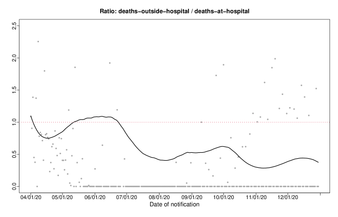
Figure 8: Estimated ratio of number of deaths (inside and outside hospital) from April to December 2020.

4.3 Examples of extrapolating the ratio of densities with an indicator $C_{2}$, the Covid-19 case of France

For any $t>0$, let $g(t)$ be the ratio of number of deaths-outside-hospital over the number of deaths-inside-hospital defined in Section 3.3, and the estimator $\widehat{g}(t)$ defined as the ratio of the two nonparametric regression estimators, that is $\widehat{g}(t)=\widehat{N}_{\rm out}(t)/\widehat{N}_{\rm in}(t)$, for all $t\in(0,T)$.

Let us imagine that we have data only until 30-September-2020 (i.e. $T$). Specifically we have observations of the number daily infections and hospitalizations, number of deaths inside hospitals, number of hospital discharges and number of persons dying outside hospitals. Our goal is to forecast the total number of deaths (inside and outside hospital) during the month of October-2020.

To do it , previously we need to forecast the number of infected and hospitalized in October-2020. So we consider our insights in Gámiz et al. (2023) where we have proposed a new methodology to forecast the number of infected in October-2020 using the two-dimensional infection rate estimated with data until 30-September-2020 and an indicator $C_{1}$ that is very close to the well known reproduction number (see Gámiz et al. (2023)). In short, we assume that the infection rate at the end of the forecasting period is the more recent estimate multiplied by $C_{1}$ and varies linearly in between. If no significant changes are expected in the immediate future with respect to the infection process, then it means that reliable predictions of the number of infected in the next period can be obtained with $C_{t}=1$. On the other hand, an optimal value of $C_{1}$ would be estimated in the infeasible in practice case that we had observations in the forecasting interval. In that case, we obtained the optimal value $C_{1}=1.542$ (see Gámiz et al. (2023)). Using this value we could obtain the predicted number of infections along the month of October closest to the real values.

Once the predicted number of infections in October are obtained, we can predict the new daily hospitalized and the number of deaths inside hospital. For this we assume that, in the forecasting interval, the hospitalization rate defined in Gámiz et al. (2023) as well as the survival hazard function defined in Section 2 are constant and equal to the most recent estimation (at time $T$), respectively. Then we obtain forecasts of the number of deaths inside hospital in the period of October 2020.

Finally, to predict the total number of deaths (inside and outside the hospital) we use the extrapolated ratio $\widetilde{g}(T+s)$ as defined in Section 3.4. Under the assumption that the ratio of number-of-deaths-outside and the number-of-deaths-inside is constant, that is, $\widetilde{g}(T+s)=\widehat{g}(T)$, for all $0<s\leq h$, we have that $C_{2}=1$. On the other hand, we can consider an infeasible in practice procedure to choose the optimal value of the constant by optimizing the predicted number of daily deaths in the target forecasting interval, that is in October-2020.

Figure 9 displays the results for our real data application of covid-19 in France. Two different forecasts for the total number of deaths in October are presented in the plot. On the one hand we consider the values predicted (green line) with the optimal value of infection indicator $C_{1}=1.542$ and the optimal survival indicator $C_{2}=2.732$. On the other hand, if no prior expert knowledge is available and we assume that in the very next future (October 2020) no significant changes in the evolution of the pandemic are expected with respect to the current situation (30-September-2020), we calculate predicted values for new infections and total number of deaths taking $C_{1}=C_{2}=1$. These values are represented by the blue curve plotted in Figure 9.

We consider the observation interval until 30-September-2020 and predict the total number of deaths in October-2020.

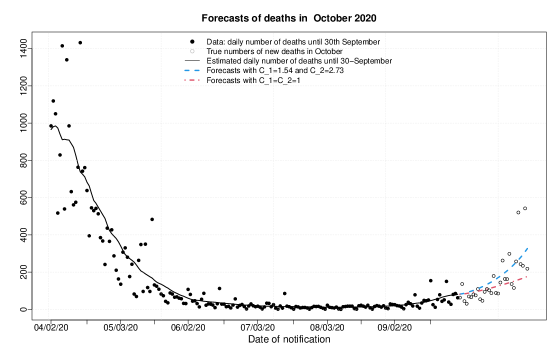
Figure 9: Total number of deaths from 1-April-2020 to 31-October-2020. The dots in the graph are the observed number of deaths inside hospitals plus observed number of deaths outside hospital until 30-September (black) and in October (grey). The estimated number of deaths until 30-September are represented by the red curve. Optimal forecasts in October are represented by the green curve. Forecast obtained with no prior knowledge are represented by the blue curve.

5 Simulations

We carry out a simulation study inspired by the practical application discussed in Section 4. First of all we assume that new arrivals in hospital occur according to a non-homogeneous Poisson process whose intensity is assumed piece-wise constant and is estimated from data. Figure 10 displays the observed number of daily accumulated arrivals to hospital and the estimated cumulative intensity curve.

Figure 10: New admissions to hospital are assumed to follow a NHPP. The stepped line are the observed accumulated daily arrivals to hospital and the solid line is the estimated cumulative intensity of the process.

Let us consider the two-dimensional hazard of survival time in hospital as $\mu_{2}(t,w)=\alpha(t)\alpha(w)$. Here $t$ refers to the notification date and $w$ is time duration in hospital.

We denote $\mu_{2}(t,w)$ the two-dimensional hazard for time duration in hospital regardless the final event is death or recovery, and assume that $\mu_{2}(t,w)=\alpha(t)\cdot\alpha(w)=\alpha(t)\left(\alpha_{1}(w)+\alpha_{2}(w)\right)$. The true hazard rates are:

1. $\alpha_{1}(t)=B(t;2,2)/T;$

2. $\alpha_{2}(t)=(0.6/T)\left\{B(t;0.5,0.5)+B(t;2,4)+B(t;4,2)\right\}$

3. $\alpha(t)=\alpha_{1}(t)+\alpha_{2}(t)$

4. $\alpha(w)=\alpha_{1}(w)+\alpha_{2}(w)$

where $t\in(0,T)$ and $B(t;a,b)$ is the density at $t$ of a Beta distribution with parameters $(a,b)$. See Figure 11.

Figure 11: True models to simulate data.

To evaluate the performance of the estimators, we have considered the following measure of the error

$$err(\widehat{\alpha}_{j,{\bf{\rm b}}})=n^{-1}\sum_{z=1}^{M}\sum_{t=1}^{M-z+1}\left(\widehat{\alpha}_{j,\bf{\rm b}}(z,t)-\alpha_{j}(z.t)\right)^{2}$$

with $j=1,2$.
The results of the simulations are presented in Table 1. Two estimates are compared: the local linear hazard estimate using full information and the hazard estimates derived from our algorithm using available data. We can see that using partial information notably increases the integrated bias and thus the $MISE$.

Table 1: Simulation results based on 500 simulations. For each case (method and sample size) the average of the $ISE$ values ($MISE$), are decomposed into squared integrated bias ($ISB$) and integrated variance ($MIV$). Numbers have been multiplied by $10^{9}$.

		Full information		Partial information
N	Criteria	Deaths	Recoveries	Deaths	Recoveries
10000	MISE	1.6755	2.8311	11.7095	9.6399
	ISB	0.6271	1.1515	9.2786	4.3358
	MIV	1.0484	1.6797	2.4309	5.304
1e+05	MISE	0.0394	0.0978	0.7396	0.3766
	ISB	0.0154	0.0601	0.6926	0.2612
	MIV	0.024	0.0376	0.047	0.1155
1e+06	MISE	0.001	0.0039	0.0699	0.0472
	ISB	4e-04	0.0022	0.0698	0.047
	MIV	5e-04	0.0017	1e-04	2e-04

6 Conclusion

This paper provides an operational approach to manage a developing pandemic based on easy to communicate and available data. The method can perhaps be understood as a benchmark method to develop in the beginning of a pandemic that can be supplemented during the pandemic by more detailed approaches based on more specific and perhaps more locally defined data. The new management approach to monitor a developing pandemic is able to separate the labour of analysis in the pure statistical forecasting methodology based on available data that can be adjusted according to prior knowledge on the infection reproduction, the $R$-number, and prior knowledge on the distribution of deaths inside and outside hospitals. This potential division of labour might be important when management has to operate fast during (and in particular in the beginning of) a pandemic.

References

- Aleman et al. (2011) Aleman, D. M., Wibisono, T. G., and Schwartz, B. 2011. A nonhomogeneous agent-based simulation approach to modeling the spread of disease in a pandemic outbreak. Interfaces, 41(3), 301-315.
- Andersen et al. (1993) Andersen, P., Borgan, O., Gill, R. and Keiding, N. 1993. Statistical Models Based on Counting Processes. New York: Springer.
- Bennouna et al. (2023) Bennouna, A., Joseph, J., Nze-Ndong, D., Perakis, G., Singhvi, D., Lami, O. S., Spantidakis, Y., Thayaparan, L., and Tsiourvas, A. 2023. COVID-19: Prediction, prevalence, and the operations of vaccine allocation. M&SOM-Manuf. Serv. Oper. Manag. 25(3) 1013–1032.
- Britton and Tomba (2019) Britton, T., and Scalia Tomba, G. 2019. Estimation in emerging epidemics: biases and remedies. J. R. Soc. Interface 16(150) 20180670.
- Cao et al. (2022) Cao, X., Zhang, D., and Huang, L. 2022. The impact of the COVID-19 pandemic on the behavior of online gig workers. M&SOM-Manuf. Serv. Oper. Manag. 24(5) 2611–2628.
- Chang and Kaplan (2023) Chang, J. T., and Kaplan, E. H. 2023. Modeling local coronavirus outbreaks. Eur. J. Oper. Res. 304(1) 57–68.
- Das et al. (2023) Das, S., Bose, I., and Sarkar, U. K. 2023. Predicting the outbreak of epidemics using a network-based approach. Eur. J. Oper. Res. 309(2) 819–831.
- De Vericourt et al (2021) De Vericourt, F., Gurkan, H., and Wang, S. 2021. Informing the public about a pandemic. Manage. Sci. 67(10) 6350–6357.
- Dean and Yang (2021) Dean, N., and Yang, Y. 2021. Discussion of “Regression Models for Understanding COVID-19 Epidemic Dynamics With Incomplete Data. J. Am. Stat. Assoc. 116 1587–1590.
- Dillon et al. (2023) Dillon, R. L., Bier, V. M., John, R. S., and Althenayyan, A. 2023. Closing the gap between decision analysis and policy analysts before the next pandemic. Decis. Anal.
- Ekici et al. (2014) Ekici, A., Keskinocak, P., and Swann, J. L. 2014. Modeling influenza pandemic and planning food distribution. M&SOM-Manuf. Serv. Oper. Manag. 16(1) 11–27. Modeling Influenza Pandemic and Planning Food Distribution
- Farahani et al. (2023) Farahani, R. Z., Ruiz, R., and Van Wassenhove, L. N. 2022. Introduction to the special issue on the role of operational research in future epidemics/pandemics. Eur. J. Oper. Res. 304(1) 1–8,
- Follmann and Fay (2021) Follmann, D., and Fay, M. 2021. Vaccine efficacy at a point in time. medRxiv, 2021-02.
- Fraser (2007) Fraser, C. 2007. Estimating Individual and Household Reproduction Numbers in an Emerging Epidemic PLoS ONE, 2(8) e758.
- Gámiz et al. (2013) Gámiz, M. L., Janys, L., Martínez-Miranda, M. D. and Nielsen, J. P. 2013. Bandwidth selection in marker dependent kernel hazard estimation Comput. Stat. Data Anal. 68 155–169.
- Gámiz et al. (2016) Gámiz, M. L., Mammen, E., Martínez-Miranda, M. D. and Nielsen, J. P. 2016. Double one-sided cross-validation of local linear hazards, J. R. Stat. Soc. Ser. B-Stat. Methodol. 78 755–779.
- Gámiz et al. (2022) Gámiz, M. L., Mammen, E., Martínez-Miranda, M. D. and Nielsen, J. P. 2022. Missing link survival analysis with applications to available pandemic data Comput. Stat. Data Anal. 169 107405.
- Gámiz et al. (2023) Gámiz, M. L., Mammen, E., Martínez-Miranda, M. D. and Nielsen, J. P. 2023. Low quality exposure and point processes with a view to the first phase of a pandemic. (Submitted.)
- Gao et al. (2020) Gao, F., Tao, L., Huang, Y., and Shu, Z. 2020. Management and data sharing of COVID-19 pandemic information. Biopreserv. Biobank. 18(6) 570–580.
- Garrett (2023) Garrett, A. (2023) “12 recommendations directed at improving preparedness for the UK’s statistical ecosystem. UK Covid-19 Inquiry.” Witness statement on behalf of Royal Statistical Society.
- Gilbert et al. (2022) Gilbert, P. B., Fong, Y., Kenny, A., and Carone, M. 2022. A controlled effects approach to assessing immune correlates of protection. Biostatistics kxac024.
- Goldenshluger and Koops (2019) Goldenshluger, A. and Koops, D. 2019. Nonparametric Estimation of Service Time Characteristics in Infinite-Server Queues with Nonstationary Poisson Input Stochastic Systems 9(3) 183–207.
- Gutiérrez and Rubli (2021) Gutierrez, E., and Rubli, A. 2021. Shocks to hospital occupancy and mortality: Evidence from the 2009 H1N1 pandemic. Manage. Sci. 67(9) 5943–5952.
- Hammami et al. (2023) Hammami, R., Salman, S., Khouja, M., Nouira, I., and Alaswad, S. 2023. Government strategies to secure the supply of medical products in pandemic times. Eur. J. Oper. Res. 306(3) 1364–1387.
- Heins et al. (2022) Heins, J., Schoenfelder, J., Heider, S., Heller, A. R., and Brunner, J. O. 2022. A scalable forecasting framework to predict COVID-19 hospital bed occupancy. INFORMS J. Appl. Anal. 52(6) 508–523.
- Ko et al. (2023) Ko, G. Y., Shin, D., Auh, S., Lee, Y., and Han, S. P. 2023. Learning Outside the Classroom During a Pandemic: Evidence from an Artificial Intelligence-Based Education App. Manage. Sci. 69(6) 3616–3649.
- Kong et al. (2021) Kong, L., Hu, K., and Walsman, M. 2021. Caring for an aging population in a post-pandemic world: Emerging trends in the US older adult care industry. Serv. Sci. 13(4) 258–274.
- Kraft and Weiss (2023) Kraft, H., and Weiss, F. 2023. Pandemic portfolio choice. Eur. J. Oper. Res. 305(1) 451–462.
- Lee et al. (2015) Lee, E. K., Yuan, F., Pietz, F. H., Benecke, B. A., and Burel, G. 2015. Vaccine prioritization for effective pandemic response. Interfaces 45(5) 425–443.
- Li et al. (2023) Li, M. L., Bouardi, H. T., Lami, O. S., Trikalinos, T. A., Trichakis, N., and Bertsimas, D. 2023. Forecasting COVID-19 and analyzing the effect of government interventions. Oper. Res. 71(1) 184–201.
- Lin (2022) Lin, X. 2022. Lessons Learned from the COVID-19 Pandemic: A Statistician’s Reflection Stat. Sci. 37 278–283.
- Liu et al. (2021) Liu, Q., Shen, Q., Li, Z., and Chen, S. 2021. Stimulating consumption at low budget: evidence from a large-scale policy experiment amid the COVID-19 pandemic. Manage. Sci. 67(12) 7291–7307.
- Liu and Hu (2022) Liu, Y., and Hu, F. 2022. Balancing Unobserved Covariates With Covariate-Adaptive Randomized Experiments J. Am. Stat. Assoc. 117(538) 875–886.
- Lu and Borgonovo (2023) Lu, X., and Borgonovo, E. 2023. Global sensitivity analysis in epidemiological modeling. Eur. J. Oper. Res. 304(1) 9–24.
- Mammen et al. (2011) Mammen, E., Martínez-Miranda, M. D., Nielsen, J. P. and Sperlich, S. 2011. Do-validation for kernel density estimation J. Am. Stat. Assoc. 106 651–660.
- Mammen and Müller (2023) Mammen, E. and Müller, M. 2023. Nonparametric estimation of locally stationary Hawkes processes Bernoulli 29(3) 2062–2083.
- Mahsin et al. (2022) Mahsin, M. D., Deardon, R., and Brown, P. 2022. Geographically dependent individual-level models for infectious diseases transmission. Biostatistics 23(1) 1–17.
- Mukherjee (2022) Mukherjee, B. 2022. Being a Public Health Statistician During a Global Pandemic Stat. Sci. 37(2) 270–277.
- Mukherjee and Seshadri (2022) Mukherjee, U. K., and Seshadri, S. 2022. Epidemic Modeling, Prediction, and Control. In Tutorials in Operations Research: Emerging and Impactful Topics in Operations (pp. 1–35). INFORMS.
- Nielsen (1998) Nielsen, J. P. 1998. Marker dependent kernel estimation from local linear estimation Scand. Actuar. J. 2 113–124.
- Nielsen and Linton (1995) Nielsen, J. P. and Linton, O. 1995. Kernel estimation in a non-parametric marker dependent hazard model Ann. Stat. 23 1735–1748.
- Nielsen and Tanggaard (2001) Nielsen, J. P., and Tanggaard, C. 2001. Boundary and bias correction in kernel hazard estimation. Scand. J. Stat. 28(4) 675–698.
- Quick et al. (2021) Quick, C., Dey, R., Lin, X. 2021. Regression Models for Understanding COVID-19 Epidemic Dynamics With Incomplete Data J. Am. Stat. Assoc. 116(536) 1561–1577.
- Rautenstrauss et al. (2023) Rautenstrauss, M., Martin, L., and Minner, S. 2023. Ambulance dispatching during a pandemic: Tradeoffs of categorizing patients and allocating ambulances. Eur. J. Oper. Res. 304(1), 239–254.
- Ru et al. (2021) Ru, H., Yang, E., and Zou, K. 2021. Combating the COVID-19 pandemic: The role of the SARS imprint. Manage. Sci. 67(9) 5606–5615.
- Rubin (1996) Rubin,D. B. 1996. Multiple imputation after 18+ years. J. Am. Stat. Assoc. 91(434) 473–489.
- Serra-García and Szech (2023) Serra-García, M., and Szech, N. 2023. Incentives and defaults can increase COVID-19 vaccine intentions and test demand. Manage. Sci. 69(2) 1037–1049.
- Slater et al. (2023) Slater, J. J., Bansal, A., Campbell, H., Rosenthal, J. S., Gustafson, P., and Brown, P. E. 2023. A Bayesian approach to estimating COVID-19 incidence and infection fatality rates. Biostatistics kxad003.
- Sparapani et al. (2020) Sparapani, R. A., Rein, L. E., Tarima, S. S., Jackson, T. A., and Meurer, J. R. 2020. Non-parametric recurrent events analysis with BART and an application to the hospital admissions of patients with diabetes. Biostatistics 21(1) 69–85.
- Thul and Powell (2023) Thul, L., and Powell, W. 2023. Stochastic optimization for vaccine and testing kit allocation for the COVID-19 pandemic. Eur. J. Oper. Res. 304(1) 325–338.
- Yin et al. (2023) Yin, X., Buyuktahtakin, I. E., and Patel, B. P. 2023. Covid-19: Data-driven optimal allocation of ventilator supply under uncertainty and risk. Eur. J. Oper. Res. 304(1) 255–275.
- Zhao et al. (2020) Zhao, J., Kim, H. J., Kim, H. M. 2020. New EM-type algorithms for the Heckman selection model Comput. Stat. Data Anal. 146 106930.