Low quality exposure and point processes with a view to the first phase of a pandemic

Abstract

In the early days of development of a pandemic there is no time for complicated data collection. One needs a simple cross-country benchmark approach based on robust data that is easy to understand and easy to collect. The recent pandemic has shown us what early available pandemic data might look like, because statistical data was published every day in standard news outlets in many countries. This paper provides new methodology for the analysis data where exposure is only vaguely understood and where the very definition of exposure might change over time. The exposure of poor quality is used to analyse and forecast events. Our example of such exposure is daily infections during a pandemic and the events are number of new infected patients in hospitals every day. Examples are given with French Covid-19 data on hospitalized patients and numbers of infected.

Keywords:Hazard; Exposure of Low Quality; Pandemic; Benchmark method

1 Introduction

During a global pandemic, development is likely to be chaotic, requiring the collection of information and knowledge from various environments daily. The outbreak might shift from one country to another, and definitions and measurements change frequently. For instance, hospitalization criteria may evolve dynamically, while the daily number of hospitalized individuals can be reliably recorded in many countries. On the other hand, the definition of exposure, such as daily infections during a pandemic, might be vaguely understood and subject to change over time. Standardization and easy exchange of both input and output are crucial in the methodology used.

Data collection time, communication and knowledge sharing across communities, quick data processing and easily understood output have been all extremely important in helping the society to understand the pandemic. Richardson (2022) argues that the new challenges posed by the pandemic have clearly highlighted how the ubiquitous nature of statistical thinking gives us the capacity to understand and model complex contexts and dynamics, dealing with constraints of agility, responsiveness and societal responsibilities.

When good quality data are available it is possible to work with complicated statistical models. Giudici et al. (2023) proposes a model using a large dataset that includes spaciotemporal, mobility and sociodemographic covariates; Samyak and Palacios (2023) apply evolutionary trees based on different subsamples of SARS-CoV-2 molecular sequences across different states of the US; Stokell et al. (2021) compares a collection of predictive models with a purpose of establishing spacial clusters in the US; in Jiang et al. (2022) the dynamics of the infection is accounted by a quantile-based approach which is robust to outliers and captures heterocedasticity; Millimet and Parmeter (2022) a model based on the SIR framework extended to allow for underreporting number of cases and deaths.

During the course of the Covid-19 pandemic data analyses have shown to be an impressive tool for decision makers. But one key question, especially at the first phase of a pandemic, is that decisions have to be made rapidly. At that stage, there is not enough time to gather very detailed data. This paper provides a new methodology introducing a dynamic approach to monitoring a pandemic with available data. The data used are simple reflecting the type of data almost every news reading person learned to know during the Covid-19 pandemic. The simplicity of the data is a mathematical statistical challenge and new missing data methodology has to be developed. The missing link between origin and end events in the available data call for new strategies. The approach presented in this paper can be used as a benchmark methodology at the beginning of a pandemic. The next section describes the strong connection between our work and the planing presented in Garrett (2023) on behalf of the Royal Statistical Society designed to prepare future societies for success in facing collective risk situations such as the recent covid-19

Efficient management of a global pandemic relies on at least two crucial aspects. Firstly, collaborative efforts must include social and environmental scientists, statisticians, and health experts. Secondly, these professionals need to divide their labour effectively. Our approach is able to include input from the valuable contributions of Storvik et al. (2022), Pellis et al. (2022), Park et al. (2020), and others, for the derivation of the reproduction number which is a crucial expert knowledge that can be used in our methodology directly for forecasting. Additionally, our work can also serve as a means to test the accuracy of the $R$-number, allowing for a productive division of labour. Experts in the $R$-number no longer need to be experts in the overall scientific modelling of the problem.

In this paper, the focus is on infection process and hospitalizations of infected patients. When modelling the transition rate from number of infected individuals to number of hospitalized, the number of individuals involved are based on some subsample of the population and even with a dynamic criteria for selecting this subsample, i.e. the number of positive tested. The new methodology of this paper is introducing a dynamic extension in various directions of the recent paper Gámiz et al. (2022) that provides a new technique solving a new missing link data problem for survival analysis and uses it on Covid-19 pandemic data.

The practical applications of the methodology developed in this paper are not limited to monitoring a pandemic. In society, forecasting events before they happen is common and exposure data is often of low quality and dynamically changing over time. There are many areas besides hospital admissions during a pandemic including crimes, insurance fraud and tax avoidance. In police crime cases, the quality of police actions in collecting local information on potential suspicious events or individuals may vary. Also for insurance fraud or tax avoidance, the quality of data collection can vary over time. A dynamic approach is therefore necessary to adjust for the time dependency in the low quality exposure information.

Let $N_{2}$ be a counting process measuring the number of events over time and let $N_{1}$ be a vaguely connected stochastic process that might impact future values of $N_{2}$. $N_{1}$ does not need to be a counting process. One key assumption in our approach is that there is a clear correlation of values of $N_{1}$ in neighbouring time points: if there is a lot going on at one time point, this will lead to high activity in the near future as well. We will model the effect from one time point of $N_{1}$ to another via a dynamic time stochastic process, equal to or related to a non stationary Hawkes process. At every time point $t$, this dynamic process is started and scaled with $N_{1}(t)$ to provide future contributions to $N_{1}$. The events $N_{2}$ are modelled via a modification of a Hawkes process starting at every time point $t$ and scaled with $N_{1}(t)$. In the pandemic case, $N_{2}$ is the number of entrances into hospital and $N_{1}$ is the number of registered infections.

The modelling of $N_{1}$ and $N_{2}$ provides a model where it is possible to forecast the future values of $N_{2}$ given the information available in $N_{1}$. However, if the model should be general enough to help monitor the development, then it should be possible to incorporate information or prior knowledge from other sources than just $N_{1}$ and $N_{2}$. The approach of this paper is able to incorporate such extra knowledge in a very simple way and via one number only. That number provides an intervention on the forecasting of $N_{1}$. We call that number $C_{t^{*},h}$, where $t^{*}$ is the most recent estimation time, $t^{*}+h$, with $h>0$, is the forecasting horizon and the value of $C_{t^{*},h}$ is the expected change of the future rate of events. If there would be no intervention and no useful prior knowledge then $C_{t^{*},h}$ is simply equal to one. If an intervention or other prior knowledge is provided indicating lower future events of $N_{2}$ then $C_{t^{*},h}$ is set to a number lower than one, and vice versa when intervention or prior knowledge indicate an increase in future events. In the pandemic case, we will show that $C_{t^{*},h}$ corresponds to the well known reproduction number, that was a daily news information in many countries during the most severe parts of the pandemic. The advantage of the approach of this paper is that it provides the difficult algorithms dealing with the modelling of the number of entrances to hospital based on the easy-to-collect and easy-to-understand information present in $N_{1}$ and $N_{2}$. Extra information to monitor and forecast can be incorporated via the well known reproduction number. Our methodology is general and apply to all the cases mentioned in the beginning of this introduction and most likely to many others.

Looking at the literature, our approach with the $N_{1}$’s can be seen as a probabilistic queueing theory approach, see for example the related paper Goldenshluger and Koops (2019), or it can be understood as a missing data problem, because we do not know the exact link between one infected and another infected, a link we would normally use while estimating stochastic processes, see Gámiz et al. (2022) for details. There is missing data interpretation also when considering the prediction or forecasting of $N_{2}$ based on $N_{1}$, also here the exact link is missing. That missing data problem is new and do not match EM-algorithms or other well known missing data approaches, see for example Heckman (1979), Rubin (1996), Zhao et al (2020), Liu and Hu (2022), Little and Rubin (2019), Kim and Shao (2021). and Gámiz et al. (2022).

The main contributions of this paper are summarized in the following. First we describe the modelling of the vaguely defined exposure measure $N_{1}$ as a Hawkes process or as a related process and provide an iterative algorithm to estimate the entering quantities. We also provide theoretical justification for our use of the estimators. Then we model the relationship between $N_{2}$ and $N_{1}$ via a modification of a Hawkes process and provide another iterative algorithm for estimation, along with the theoretical justification of the estimators. To provide forecasts we introduce our principles of incorporating extra information or prior knowledge into our system via our simple constant $C_{t^{*},h}$. Finally, we provide a complete case study including the modelling of $N_{1}$ and $N_{2}$ and the use of extra information or prior knowledge. Our example is the Covid-19 pandemic in France and the prior knowledge is the weekly published reproduction number of infections.

The simplicity of the structure of our methodology makes the method useful to other applications than the important special case of pandemic data. In the conclusion section we will add some comments on the relationship of our method to some of the key developments of statistical methodology on infections data published when the Covid-19 pandemic was at its height.

The organisation of the paper is as follows. Section 3 provides methodology to monitor the feedback loop of the vaguely defined exposure process. Section 2 we establish a strong connection to the strategies proposed by the Royal Statistical Society focused on the preparedness of the UK’s statistical and data ecosystem to effectively address potential collective risks that may arise in the future. Section 4 provides methodology to connect the events of interest to the vaguely defined exposure process. Section 5 shows how the methodology of Section 3 and Section 4 can be used for forecasting conveniently adding only one number from prior knowledge or other sources. Section 6 goes through the methodology of Section 3 and Section 4 using available French Covid-19 data and Section 7 shows how to combine the methodology of Section 5 with the results of Section 6 to forecast hospitalizations in a developing pandemic. Finally, Section 8 provides the conclusions of the paper and establishes connections with some of the recent methodological papers on the Covid-19 pandemic.

2 Royal Statistical recommendations directed at improving preparedness for the UK’s statistical ecosystem

In this section we link our new approach to the recent guidelines from Royal Statistical Society on preparedness for the next pandemic, see Garrett (2023). In the evaluation of Garrett (2023), Section 4.3.1, it is noted that “During a pandemic, the government needs to make policy decisions based on imperfect and changing information.” and further “While details are difficult to prescribe in advance of a pandemic, it is important that an evaluative framework is considered as part of preparedness planning”. In other words, the Royal Statistical Society recommends that a robust dynamic approach is available in the beginning of a pandemic that is able to provide reliable early results without too much detailed information. This is exactly the purpose of this paper in the case of predicting measured infections and their dynamic impact on hospitalizations. It is also noted in Garrett (2023) in Section 4.5.1 that “Communication during a pandemic is of utmost importance. When referring to data, transparency and clarity in government communication is vital for maintaining public confidence” and “Being prepared to communicate data effectively should be a core part of preparedness plans”. These comments are fully aligned with what this paper aims to do. We use only the kind of data that we know (from following the last Covid-19 pandemic) are well understood across countries and regions. This is also in line with Section 2 in Garrett (2023) on data infrastructure, where it is pointed out in Section 2.1.1 that “Data also enables effective communication with the public”. It is therefore vital that there is a direct connection between data that is easily understood and the statistical analysis. The new missing data methodology provided in this paper is therefore important for the preparedness of the next pandemic when we want to be able to communicate quickly and without misunderstandings between countries and regions and various scientists about the dynamic development of the pandemic. Without this new missing link data analysis, the data collection becomes more detailed with more possibilities for errors and misunderstandings between scientists and with the risk that the public and government bodies get lost in the discussion.

In Section 4.2.2. of Garrett (2023) it is noted that“Prepare mechanisms for engaging expert statisticians with skills in both data analysis and study design” is important. It is strongly recommended that policymakers rely on a team of statisticians. Our new benchmark method also introduces a potential division of labour while working with pandemic statistics allowing crucial input to be fed to the model via prior knowledge from external experts.

3 Modelling the feedback loop of the vaguely defined exposure measure

In this section we focus on the vaguely defined exposure process $N_{1}$. We define a model for $N_{1}$ based on Hawkes processes and propose a new estimator that works when we know the exact link between new values of $N_{1}$ and old values of $N_{1}$. To align our vocabulary to our motivating example and to help the intuition of the reader, we define new increases in $N_{1}$ as new “infections” and the value of $N_{1}$ at any point as number-of-infections. Notice that in our motivating example $N_{1}$ is not the number of infections in the population, but the registered number of infections. But to ease the reading we use the short-hand “infections”. With this new vocabulary, we could simply have used the title “Modelling the feedback loop from infection to infection” for this section.

First we describe a model for the infection rate. Then we propose a new estimator that works when we have individual follow up and thus information is registered of the time since one person is infected until he/she causes a new infection. In the following, we will refer to this situation with the term “full information”. Finally, we present an algorithm able to generate information of the time-from-infected-to-infected from available data.

3.1 Model formulation

We observe $n$ individuals in the interval $(0,T]$. Let $N_{1}(t)$ count the number of persons getting infected in the interval $(0,t]$, for $0<t\leq T$. Also, we denote $N_{1}({\mathrm{d}}t)$ the number of persons infected in the interval $(t,t+{\mathrm{d}}t]$, then $N_{1}(t)=\int_{0}^{t}N_{1}({\mathrm{d}}s)$, for $t\in(0,T]$. Furthermore, we write $N_{1}({\mathrm{d}}t,{\mathrm{d}}s)$ for the number of pairs of persons where person 1 was infected in $(s,s+{\mathrm{d}}s]$ and person 2 was infected by person 1 in $(t,t+{\mathrm{d}}t]$, and $N_{1}(t,{\mathrm{d}}s)$ for the number of persons infected in $(s,t]$ by a person that was infected at time $s$, with $s<t\leq T$.

We define ${\mathcal{F}}_{1}(t)$ as the $\sigma$-field generated by $\{N_{1}(s):s<t\}$, and

$$\lambda_{1}(t)=\lim_{{\mathrm{d}}t\rightarrow 0}\frac{P(N_{1}(t+{\mathrm{d}}t)-N_{1}(t)\geq 1\mid{\mathcal{F}}_{1}(t))}{{\mathrm{d}}t},\ 0<t\leq T.$$

Then $\lambda_{1}(t){\mathrm{d}}t={\rm E}[N_{1}({\mathrm{d}}t)\mid{\mathcal{F}}_{1}(t)]$ is the probability that one person is infected in the interval $(t,t+{\mathrm{d}}t]$ given ${\mathcal{F}}_{1}(t)$.

For the dynamics of $N_{1}(t)$ we assume that

$$\lambda_{1}(t){\mathrm{d}}t=\left(\int_{0}^{t^{-}}\mu_{1}(t/T,t-s)N_{1}({\mathrm{d}}s)\right){\mathrm{d}}t+n\rho_{1}(t){\mathrm{d}}t$$ (1)

where $\rho_{1}$ and $\mu_{1}$ are some unknown functions. We assume that $\mu_{1}(t/T,v)=0$, for $v<0$, $v>D_{1}$ and that $\rho_{1}(t)=0$, for $t>D_{1}^{\prime}$, where $D_{1}$ and $D_{1}^{\prime}$ are some fixed constants. We have that with $0\leq s<t\leq T$, $\mu_{1}({t}/{T},t-s){\mathrm{d}}t$ is the probability that a person infected at $s$ infects a person in $(t,t+{\mathrm{d}}t]$.

The function $\rho_{1}$ could be chosen for instance as $\rho_{1}(t)=\int_{-\infty}^{0}\mu_{1}({t}/{T},t-v)\nu_{1}({\mathrm{d}}v)$, where $n\nu_{1}(t)$ are the values of $N_{1}(t)$ in the past $\{N_{1}(t):t<0\}$. If we condition on the past, we can treat $\rho_{1}$ in this example as if it is a deterministic function. Note that in this case we see that $\rho_{1}(t)=0$, for $t>D_{1}$ because $\mu_{1}(t/T,w)=0$ for $w>D_{1}$. In the following we allow arbitrary specifications of $\rho_{1}$.

According to equation (1), $N_{1}(t)$ is a locally stationary Hawkes process (Mammen and Müller, 2023). Our aim is to estimate $\mu_{1}(t/T,w)$, for $0<t<T$ and $0<w<D_{1}$. Ideally, to do it we have observations of the process $N_{1}(t,{\mathrm{d}}s)$. However in our motivating problem we only observe the process $N_{1}(t)$. In the next section we describe the estimation of $\mu_{1}(t/T,w)$ in the case we had observed $N_{1}({\mathrm{d}}t,{\mathrm{d}}s)$, for all $s<t\leq T$. Afterwards we propose an algorithm which is able to estimate $N_{1}({\mathrm{d}}t,{\mathrm{d}}s)$ from the observations of $N_{1}(t)$.

3.2 Estimator of the two-dimensional transition intensities when full information is available

With full information we observe the process $N_{1}(t,{\mathrm{d}}s)$ for $s<t\leq T$. For $s$ fixed, $N_{1}(t,{\mathrm{d}}s)$ is a counting process with respect to (an increasing, right continuous, complete filtration) $\mathcal{F}_{1}(t)$ , $t\in(0,T)$. We are interested in estimating the two-dimensional intensity $\mu_{1}(t/T,t-s)$ with no restriction on its functional form. We consider the two-dimensional local linear estimator given by:

$$\widehat{\mu}_{1}(t/T,t-s)=\frac{\int_{0\leq v<u\leq T}{\rm C}_{1}(s,t,v,u)\ K_{1,b_{1}}\left(\frac{t-u}{T}\right)K_{2,b_{2}}(t-s-(u-v))N_{1}({\mathrm{d}}u,{\mathrm{d}}v)}{\int_{0\leq v<u\leq T}{\rm C}_{1}(s,t,v,u)\ K_{1,b_{1}}\left(\frac{t-u}{T}\right)K_{2,b_{2}}(t-s-(u-v))N_{1}({\mathrm{d}}v)\ {\mathrm{d}}u},$$ (2)

with $N_{1}({\mathrm{d}}u,{\mathrm{d}}v)$ and $N_{1}({\mathrm{d}}v)$ as defined previously, for $i=1,\ldots,n$.

Notice that the estimator is a ratio of a local linear estimator of occurrences and a local linear estimator of exposure. This is similar to local linear marker dependent kernel hazard estimation in survival analysis, see Nielsen and Linton (1995) for the local constant case and Nielsen (1998) for the local linear case (see also Gámiz et al. (2013) for the problem of the bandwidth selection in this context).

In (2) we have used the following notation: For $j=1,2$, $K_{j,b_{j}}(\cdot)=K_{j}(\cdot/b_{j})/b_{j}$, where $K_{j}$ is a general one-dimensional kernel function. We denote

$${\rm C}_{1}(s,t,v,u)=1-\big{(}(t-u)/T,t-s-(u-v)\big{)}^{t}{\rm{\bf A}}(t,s)^{-1}{\rm{\bf a}}(t,s)$$ (3)

for $0\leq s<t\leq T$. Here ${\rm{\bf a}}$ is a vector function whose $l$-th component is

$${\rm a}_{l}(t,s)=\int_{0\leq v<u\leq T}\!K_{1,b_{1}}\left(\frac{t-u}{T}\right)K_{2,b_{2}}(t-s-(u-v))$$

$$\qquad\qquad\times\left(\frac{t-u}{T}\right)^{\delta_{l1}}(t-s-(u-v))^{\delta_{l2}}N_{1}({\mathrm{d}}v)\ {\mathrm{d}}u$$ (4)

for $l=1,2$ and $s<t<T$, with $\delta_{lh}=1$ if $l=h$, and 0, otherwise; and ${\rm{\bf A}}$ is a matrix function of dimension $2\times 2$ whose $(l,m)$-element is given by

$${\rm A}_{l,m}(t,s)=\int_{0\leq v<u\leq T}\!K_{1,b_{1}}\left(\frac{t-u}{T}\right)K_{2,b_{2}}(t-s-(u-v))$$

$$\quad\times\left(\frac{t-u}{T}\right)^{\delta_{l1}+\delta_{m1}}(t-s-(u-v))^{\delta_{l2}+\delta_{m2}}N_{1}({\mathrm{d}}v)\ {\mathrm{d}}u,$$ (5)

for $l,m=1,2$, with $\delta_{lh}$ defined above, and $\delta_{mh}=1$ if $m=h$ and 0 otherwise.

3.3 An iterative estimation scheme approximating the infeasible estimator of the last subsection

We now describe an iterative estimation scheme for the estimation of $\mu_{1}$. At the $r$th iteration of the algorithm we have an estimated value of $\mu_{1}$ from the last iteration that we denote by $\widehat{\mu}_{1}^{(r-1)}$. For $r=1$ we use an initial guess $\widehat{\mu}_{1}^{(0)}$ of $\mu_{1}$. The $r$th iteration of the algorithm consists of two steps. In the first step we construct a two-dimensional process $\hat{N}^{(r)}(t,{\mathrm{d}}s)$ that approximates $N_{1}(t,{\mathrm{d}}s)$. This is done by using the estimator $\widehat{\mu}_{1}^{(r-1)}$ from the previous iteration and by using the observed process $N_{1}(t)$:

$$\hat{N}_{1}^{(r)}({\mathrm{d}}u,{\mathrm{d}}v)=\frac{\hat{\mu}_{1}^{(r)}(u/T,u-v)}{\int_{0}^{u^{-}}\hat{\mu}_{1}^{(r)}(u/T,u-w)N_{1}({\mathrm{d}}w)}N_{1}({\mathrm{d}}v)N_{1}({\mathrm{d}}u).$$ (6)

In the second step, this estimator of $N_{1}({\mathrm{d}}u,{\mathrm{d}}v)$ is plugged into (2). This results in the following update of $\widehat{\mu}_{1}^{(r)}$:

$$\widehat{\mu}_{1}^{(r+1)}(t/T,t-s)=\frac{\int_{0\leq v<u\leq T}{\rm C}_{1}(s,t,v,u)\ K_{1,b_{1}}\left(\frac{t-u}{T}\right)K_{2,b_{2}}(t-s-(u-v))\hat{N}_{1}^{(r)}({\mathrm{d}}u,{\mathrm{d}}v)}{\int_{0\leq v<u\leq T}{\rm C}_{1}(s,t,v,u)\ K_{1,b_{1}}\left(\frac{t-u}{T}\right)K_{2,b_{2}}(t-s-(u-v))N_{1}({\mathrm{d}}v)\ {\mathrm{d}}u}.$$ (7)

If this iteration scheme converges it will converge against the solution $\hat{\mu}_{1}(t/T,t-s)$ of the equation:

$$\hat{\mu}_{1}(t/T,t-s)=\int_{0\leq v<u\leq T}{\rm C}_{1}(s,t,v,u)K_{1,b_{1}}\left(\frac{t-u}{T}\right)K_{2,b_{2}}(t-s-(u-v))$$

$$\qquad\times\frac{\hat{\mu}_{1}(u/T,u-v)}{\int_{0}^{u^{-}}\hat{\mu}_{1}(u/T,u-w)N_{1}({\mathrm{d}}w)}N_{1}({\mathrm{d}}v)N_{1}({\mathrm{d}}u)$$ (8)

$$\qquad\times\frac{1}{\int_{0\leq v<u\leq T}{\rm C}_{1}(s,t,v,u)K_{1,b_{1}}\left(\frac{t-u}{T}\right)K_{2,b_{2}}(t-s-(u-v))N_{1}({\mathrm{d}}v){\mathrm{d}}u}.$$

In the next subsection we will argue that $\hat{\mu}_{1}(t/T,t-s)$ is a consistent estimator.

3.4 Asymptotic analysis

In this subsection we will argue that $\hat{\mu}_{1}(t/T,t-s)$ is a consistent estimator. This will be done in an asymptotic framework where the factor $n$ converges together with $T$ to infinity. We will see that $n$ is the order of the number of infections in a finite interval, under the assumptions that we specify now. For stating the assumptions we will make use of the martingale $M_{1}$ defined by

$$M_{1}({\mathrm{d}}t)=N_{1}({\mathrm{d}}t)-\lambda_{1}(t){\mathrm{d}}t,$$

see Andersen et al. (1993).

Furthermore, put

$$\chi_{1}(t/T,t-s)=\sum_{k=1}^{\infty}\mu_{1}^{(*k)}(t/T,t-s)$$

with $\mu_{1}^{(*k)}(t/T,t-s)=\int_{0}^{t}\mu_{1}(t/T,t-v)\mu_{1}^{(*(k-1))}(v/T,v-s){\mathrm{d}}v$, and $\mu_{1}^{(*1)}(t/T,t-s)=\mu_{1}(t/T,t-s)$. By iterative application of the Hawkes model equation one can show that

$$\Lambda_{1}(t) = {\rm E}[\lambda_{1}(t)]=n\rho_{1}(t)+n\int_{0}^{t}\chi_{1}(t/T,t-u)\rho_{1}(u){\mathrm{d}}u,$$

$$N_{1}({\mathrm{d}}t) = M_{1}({\mathrm{d}}t)+{\mathrm{d}}t\ \bigg{(}\int_{0}^{t^{-}}\chi_{1}(t/T,t-u)M_{1}({\mathrm{d}}u)+n\rho_{1}(t)$$

$$\qquad+n\int_{0}^{t}\chi_{1}(t/T,t-u)\rho_{1}(u){\mathrm{d}}u\bigg{)}.$$

We assume that the term $\int_{0}^{t}\chi_{1}(t/T,t-u)\rho_{1}(u){\mathrm{d}}u$ is bounded away from 0 and from infinity on the interval $[0,T]$. In particular, this gives that the number of infections in a finite interval is of order $n$.

We consider the estimator $\hat{\mu}_{1}(t/T,t-s)$ at point $t=Tx_{0}$, for a fixed choice $0<x_{0}<1$. We assume that the bandwidths $b_{1}$ and $b_{2}$ are converging to 0. If $\hat{\mu}_{1}$ is continuous with respect to its first and second argument we get that $\hat{\mu}_{1}(u/T,u-v)\approx\hat{\mu}_{1}(t/T,t-s)$, for $u$ and $v$ in the range of integration in the right hand side of equation (8). Thus, $\hat{\mu}_{1}$ approximately solves

$$1 \approx \int_{0\leq v<u\leq T}{\rm C}_{1}(s,t,v,u)K_{1,b_{1}}\left(\frac{t-u}{T}\right)K_{2,b_{2}}(t-s-(u-v))$$

$$\qquad\times\frac{N_{1}({\mathrm{d}}v)N_{1}({\mathrm{d}}u)}{\int_{0}^{u^{-}}\hat{\mu}_{1}(u/T,u-w)N_{1}({\mathrm{d}}w)}$$

$$\qquad\times\frac{1}{\int_{0\leq v<u\leq T}{\rm C}_{1}(s,t,v,u)K_{1,b_{1}}\left(\frac{t-u}{T}\right)K_{2,b_{2}}(t-s-(u-v))N_{1}({\mathrm{d}}v){\mathrm{d}}u}.$$

We now write $\hat{\mu}_{1}(u-w)$ for $\hat{\mu}_{1}(t_{0}/T,u-w)$ and similarly, $\mu_{1}(u-w)$ for $\mu_{1}(t_{0}/T,u-w)$, and $\chi_{1}(u-w)$ for $\chi_{1}(t_{0}/T,u-w)$. Using (3.4) one can show that

$$n^{-1}N_{1}({\mathrm{d}}t)\approx((\chi_{1}*\rho_{1})(t)+\rho_{1}(t)){\mathrm{d}}t=(\chi_{1}*\rho_{1})(t){\mathrm{d}}t$$

for $t/T$ in a small enough neighbourhood of $x_{0}$ where $(\chi_{1}*\rho_{1})(t)=\int_{0}^{t}\chi_{1}(t-w)\rho_{1}(w){\mathrm{d}}w$ denotes the convolution of $\chi_{1}$ and $\rho_{1}$ . This gives

$$1 \approx \int_{0\leq v<u\leq T}{\rm C}_{1}(s,t,v,u)K_{1,b_{1}}\left(\frac{t-u}{T}\right)K_{2,b_{2}}(t-s-(u-v))$$

$$\qquad\times\frac{(\chi_{1}*\rho_{1})(v){\mathrm{d}}v\ (\chi_{1}*\rho_{1})(u){\mathrm{d}}u}{(\hat{\mu}_{1}*\chi_{1}*\rho_{1})(u)}$$

$$\qquad\times\frac{1}{\int_{0\leq v<u\leq T}{\rm C}_{1}(s,t,v,u)K_{1,b_{1}}\left(\frac{t-u}{T}\right)K_{2,b_{2}}(t-s-(u-v))(\chi_{1}*\rho_{1})(v){\mathrm{d}}v{\mathrm{d}}u}.$$

We now remark that because $\mu_{1}(u)$ is equal to $0$, for $u>D_{1}$, we get for $t/T$ in a small enough neighbourhood of $x_{0}$ that

$$(\chi_{1}*\rho_{1})(t)=((\mu_{1}+\mu_{1}*\chi_{1})*\rho_{1})(t)=(\mu_{1}*\chi_{1}*\rho_{1})(t)+(\mu_{1}*\rho_{1})(t)=(\mu_{1}*\chi_{1}*\rho_{1})(t).$$

This gives that

$$0 \approx \int_{0\leq v<u\leq T}{\rm C}_{1}(s,t,v,u)K_{1,b_{1}}\left(\frac{t-u}{T}\right)K_{2,b_{2}}(t-s-(u-v))$$

$$\qquad\times\frac{((\hat{\mu}_{1}-\mu_{1})*\chi_{1}*\rho_{1})(u)}{(\hat{\mu}_{1}*\chi_{1}*\rho_{1})(u)}(\chi_{1}*\rho_{1})(v){\mathrm{d}}v\ {\mathrm{d}}u.$$

In particular, we see that $\mu_{1}$ is an approximate solution of equation (8). If we could show that all approximate solutions of (8) are approximately equal, this could be used to show consistency of $\hat{\mu}_{1}$. In particular this would require a precise asymptotic definition of “$\approx$” in the above equations.

For the asymptotic study of our estimator it is helpful to assume that $N_{1}$ is a Hawkes process. But essentially we only use that ${\rm E}[N_{1}({\mathrm{d}}t)\mid{\mathcal{F}}_{1}(t)]=\left(\int_{0}^{t^{-}}\mu_{1}(t/T,t-s)N_{1}({\mathrm{d}}s)\right){\mathrm{d}}t$ + $n\rho_{1}(t){\mathrm{d}}t$, where not necessarily $N_{1}({\mathrm{d}}t)$ must be $\leq 1$ almost surely. In the case of epidemic data one may wish to allow for super spreader events which would mean that $N_{1}({\mathrm{d}}t)\gg 1$. In this case one has to deviate from a Hawkes model. On the other side for large values of $n$ these differences may not be significant after discretization of the data. In the next section we will see that we have to deviate from a Hawkes model if we use $N_{1}$ to model exposure for another process $N_{2}$.

4 Modelling the relationship between the vaguely defined process, $N_{1}$, and the events of interest, $N_{2}$

In the previous sections, we considered a good model of $N_{1}$. In this section, we turn to the modelling of $N_{2}$ that is the process that we really want to model. When modelling and forecasting $N_{2}$, we will take advantage of the available information of $N_{1}$ and its modelling. To ease the vocabulary throughout, we will take advantage of the intuition of our motivating example and call increases in $N_{2}$ for “hospitalizations”. A new title of this Section 4 with this adjusted vocabulary could therefore have been the more intuitive “Modelling the transition from infected to hospitalization”.

In this section we build a model for the relationship between the infection process $N_{1}$ and the hospitalization process $N_{2}$. A new method is also proposed to estimate when information about the time length since infection to hospitalization is available.

4.1 Model formulation

We observe $n$ individuals in the interval $(0,T]$. Let $N_{2}(t)$ count the number of persons hospitalized in the interval $(0,t]$, and $N_{2}({\mathrm{d}}t)$ the number of hospitalized in the interval $(t,t+{\mathrm{d}}t]$. Then $N_{2}(t)=\int_{0}^{t}N_{2}({\mathrm{d}}u)$, for $0<t\leq T$. Furthermore, we write $N_{2}({\mathrm{d}}t,{\mathrm{d}}s)$ for the number of persons hospitalized in $(t,t+{\mathrm{d}}t]$ that had been infected in $(s,s+{\mathrm{d}}s]$, and $N_{2}(t,{\mathrm{d}}s)$ for the number of persons infected in $s,{\mathrm{d}}s]$ that enter the hospital in the interval $(s,t]$, $s<t\leq T$.

Let us define

$$\lambda_{2}(t)=\lim_{{\mathrm{d}}t\rightarrow 0}\frac{P(N_{2}(t+{\mathrm{d}}t)-N_{2}(t)\geq 1\mid{\mathcal{F}}_{1}(t))}{{\mathrm{d}}t},\ 0<t\leq T,$$

where ${\mathcal{F}}_{1}(t)$ is the $\sigma$-field generated by $\{N_{1}(s):s<t\}$, with $N_{1}$ given in Section 3.1. Then $\lambda_{2}(t){\mathrm{d}}t={\rm E}[N_{2}({\mathrm{d}}t)\mid{\mathcal{F}}_{1}(t)]$ is the probability that one person is hospitalized in the interval $(t,t+{\mathrm{d}}t]$ given ${\mathcal{F}}_{1}(t)$. We assume that

$$\lambda_{2}(t){\mathrm{d}}t=\left(\int_{0}^{t^{-}}\mu_{2}(t/T,t-s)N_{1}({\mathrm{d}}s)\right){\mathrm{d}}t+n\rho_{2}(t){\mathrm{d}}t,$$ (9)

with $\rho_{2}$ and $\mu_{2}$ some unknown functions such that $\mu_{2}(t/T,v)=0$, for $v<0$ and $v>D_{2}$, and $\rho_{2}(t)=0$ for $t>D^{\prime}_{2}$, with $D_{2},D^{\prime}_{2}$ some fixed constants, and where, for a person, who was infected at $s$, $\mu_{2}({t}/{T},t-s){\mathrm{d}}t$ is the probability that this person is hospitalized in $(t,t+{\mathrm{d}}t]$.

From equation (9), $N_{2}(t)$ would be a Hawkes process if we would replace ${\mathcal{F}}_{1}(t)$ by the $\sigma$-field generated by $\{(N_{1}(s),N_{2}(s)):s<t\}$. With this modification the assumption (9) is too restrictive. Typically $N_{2}(s)$ contains information about the future development of $N_{2}$. Consider e.g. in a thought experiment the unrealistic case that at a certain date all infected individuals are hospitalized. Then it can be expected that the number of additional hospitalizations in the next days will be low. Fitting model (9) can be used to predict future hospitalizations. The prediction depends then only on the history of $N_{1}$. In most settings neglecting the history of $N_{2}$ will only lead to a small loss of accuracy, at least if $n$ is large. Furthermore, it would be very complex to model future developments of $N_{2}$ using the history of $N_{1}$ and $N_{2}$.

4.2 Estimating the transition intensity from infected to hospitalized

We now describe an iterative estimation scheme for the estimation of $\mu_{2}$. The procedure uses a similar approach as for the estimation of $\mu_{1}$, discussed in the last section. At the $r$th iteration of the algorithm we have an estimated value of $\mu_{2}$ from the last iteration that we denote by $\widehat{\mu}_{2}^{(r-1)}$. For $r=1$ we use an initial guess $\widehat{\mu}_{2}^{(0)}$ of $\mu_{2}$. The $r$th iteration of the algorithm consists of two steps. In the first step we construct a two-dimensional process $\hat{N}_{2}^{(r)}(t,{\mathrm{d}}s)$ that approximates $N_{2}(t,{\mathrm{d}}s)$. This is done by using the estimator $\widehat{\mu}_{2}^{(r-1)}$ from the previous iteration and by using the observed processes $N_{1}(t)$ and $N_{2}(t)$, compare (6):

$$\hat{N}_{2}^{(r)}({\mathrm{d}}u,{\mathrm{d}}v)=\frac{\hat{\mu}_{2}^{(r)}(u/T,u-v)}{\int_{0}^{u^{-}}\hat{\mu}_{2}^{(r)}(u/T,u-w)N_{1}({\mathrm{d}}w)}N_{1}({\mathrm{d}}v)N_{2}({\mathrm{d}}u).$$

In the second step, we proceed similarly as in getting the update of $\widehat{\mu}_{1}^{(r+1)}$ in (7):

$$\widehat{\mu}_{2}^{(r+1)}(t/T,t-s)=\frac{\int_{0\leq v<u\leq T}{\rm C}_{1}(s,t,v,u)\ K_{1,b_{1}}\left(\frac{t-u}{T}\right)K_{2,b_{2}}(t-s-(u-v))\hat{N}_{2}^{(r)}({\mathrm{d}}u,{\mathrm{d}}v)}{\int_{0\leq v<u\leq T}{\rm C}_{1}(s,t,v,u)\ K_{1,b_{1}}\left(\frac{t-u}{T}\right)K_{2,b_{2}}(t-s-(u-v))N_{1}({\mathrm{d}}v)\ {\mathrm{d}}u}.$$

If the algorithm converges the limit $\widehat{\mu}_{2}$ of $\widehat{\mu}_{2}^{(r)}$ solves

$$\hat{\mu}_{2}(t/T,t-s)=\int_{0\leq v<u\leq T}{\rm C}_{1}(s,t,v,u)K_{1,b_{1}}\left(\frac{t-u}{T}\right)K_{2,b_{2}}(t-s-(u-v))$$

$$\qquad\times\frac{\hat{\mu}_{2}(u/T,u-v)}{\int_{0}^{u^{-}}\hat{\mu}_{2}(u/T,u-w)N_{1}({\mathrm{d}}w)}N_{1}({\mathrm{d}}v)N_{2}({\mathrm{d}}u)$$

$$\qquad\times\frac{1}{\int_{0\leq v<u\leq T}{\rm C}_{1}(s,t,v,u)K_{1,b_{1}}\left(\frac{t-u}{T}\right)K_{2,b_{2}}(t-s-(u-v))N_{1}({\mathrm{d}}v){\mathrm{d}}u}.$$

Compare (8). The performance of this estimator can be discussed by using similar arguments as that of $\hat{\mu}_{1}$ in the last section. In particular this concerns the asymptotic analysis.

5 Principles of forecasting in a dynamic environment

Forecasting is of course always tricky. Let us define an indicator (denoted later by $C_{t,h}$) indicating at any point in time $t$ whether the future ($t+h$, $h>0$) will be different or equal to the immediate past. If this indicator equals one then we can forecast the immediate future based on the immediate past. There might be periods where little is happening (and the indicator might have a tendency to increase slowly) and there might be few but very important change-points where measures (e.g. lock down) are introduced to minimize future infections (and the indicator might drop dramatically in a matter of days).

Let $t^{*}$ be the calendar time for the most recent estimate. From the observed data (until $t^{*}$) we can estimate the dynamic infection rate as $\widehat{\mu}_{1}\left(t/T,u\right)$, for $0<u\leq t\leq t^{*}$.

Let us fix the forecast horizon at time $t^{*}+h$, for an $h>0$. We need to extrapolate the dynamic infection rate $\mu_{1}\left((t^{*}+s)/T,u\right)$, for $u\geq 0$ and $0<s\leq h$. We assume that the infection rate at the end of the forecasting period is the more recent estimate multiplied by $C_{t^{*},h}$, and it varies linearly in between

$$\widetilde{\mu}_{1}\left((t^{*}+s)/T,u\right)=\widehat{\mu}_{1}\left(t^{*}/T,u\right)\times\left(1+(C_{t^{*},h}-1)\frac{s}{h}\right),$$ (10)

for $0\leq s\leq h$ and $u\geq 0$.

One can monitor and forecast with $C_{t^{*},h}$ equals one. And one can use prior knowledge (e.g. knowledge of intervention) to forecast with a $C_{t^{*},h}$ different from one. A case study of Covid-19 in France will be carried out in the next section. In this case study most of the dynamic is happening from infection to infection and one can therefore concentrate prior knowledge around this transition, while keeping the transition from infection to hospitalization unaffected by prior knowledge.

In that situation a dynamic statistical methodology as introduced in this paper can do the job via a surprisingly simple data collection reflecting what can be considered “available data” in many countries. Therefore, the only thing left to monitor and forecast well is to have a dynamic point of view and the constant $C_{t^{*},h}$. That work needs expert advice specific to countries or local regions within countries. This important work cannot be dismissed via a statistical analysis based on simplified available data. But it is important that the experts involved should only consider forecasting and understand the $C_{t^{*},h}$ rather than being responsible for a full statistical model.

In our data example we considered the so called reproduction number, or simply R number, that is defined as the expected number of new infections caused by an infectious individual (Fraser, 2007). Estimates of the actual Covid-19 reproduction numbers have been publicly reported in most countries. In the next section we will discuss choosing $C_{t^{*},h}$ such that the reproduction number of $\widetilde{\mu}_{1}$, given by

$$\int\widetilde{\mu}_{1}\left((t^{*}+s)/T,u\right){\mathrm{d}}u=\int\widehat{\mu}_{1}\left(t^{*}/T,u\right){\mathrm{d}}u\times\left(1+(C_{t^{*},h}-1)\frac{s}{h}\right)$$

is equal to the reported estimated reproduction number for $s=h$.

6 Estimating with available data. The Covid-19 case of France

In this section we combine a model of the development of observed infected in the population, as described in Section 3, with the model linking the observed number of infections to the number of arrivals to the hospital, as described in Section 4.

Based on the methodology of Section 3, we estimate the transition loop from number of observed infected to future number of observed infected to get the transition rates given in Figure 1. And based on the methodology in Section 4 we estimated the transition from number of observed infected to number of hospitalizations giving us the transition rates in Figure 2. The numerical calculation of the continuous integrals presented in Section 3 and Section 4 is done via discrete approximations to these integrals based on our available daily observations, similarly to Gámiz et al. (2013). Furthermore, optimal bandwidths have been estimated for simplicity using the cross-validation method described in Gámiz et al. (2013). This method worked well for this application otherwise other methods with better properties such as the Do-validation method of Gámiz et al. (2016) could be used, with a higher computational cost (see also Mammen et al. (2011)).

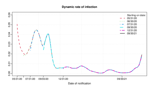
Figure 1: Dynamic estimation of the rate of infection. Each line on the plot gives the estimated intensity of the infection process that starts on the date indicated by the corresponding legend. In the notation of the paper these are estimations of $\mu_{1}(\frac{t}{T},t-s)$, plotted for $t>s$, at six calendar times $s$ taken from May 2020 to December 2021.

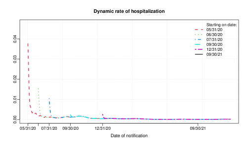
Figure 2: Dynamic estimation of the rate of hospitalization. Each line on the plot gives the estimated hospitalization rate for individuals infected on the date indicated by the corresponding legend. In the notation of the paper these are estimations of $\mu_{2}(\frac{t}{T},t-s)$, plotted for $t>s$, at six calendar times $s$ taken from May 2020 to December 2021.

In Figures 1 and 2 we can visualize the dynamics of the infections and hospitalizations, respectively, during the French Covid-19 pandemic. A steep decline in the number of cases in both May and November 2020 is noticeable in Figure 1, which can be explained as a result of the severe social restrictions that were imposed in France at those moments in time. Figure 2 shows a perhaps surprising issue: a sharp descending trend of the hospitalization rates when are seen as a function of the date of onset. That is, about 4% of new cases is estimated to be hospitalized on the 31st of May 2020; after the 30th of June same year there will be around 2%; and below 0.5% in 2021. This might suggest a slowdown in the speed of arrivals to hospital with time which may be strange given the dramatic increase in number of cases in the last period, but can be explained due to several factors. One could be the effect of the vaccines and other the successive variants of the virus which were spreading faster but were less lethal.

7 Principles of forecasting. The Covid-19 case of France

In this section we combine the methodology of Section 6, modelling vaguely defined observed infections and their implied number of hospitalizations, to a full forecasting methodology as described in Section 5. This section therefore provides us with a full forecasting methodology of number of hospitalizations.

When looking at the full system described above for the Covid-19 case of France, one can take that point of view that all transitions except that one from the infection indicator to the infection indicator can be described via slowly moving continuous development over time. In other words: except for this one transition, it makes sense - at any given date - to forecast the immediate future structure of these transitions from the immediate past. We are therefore left with the challenge of forecasting the transition from infection indicator to infection indicator. Here we use the $C_{t,h}$ explained in Section 5.

7.1 Forecasting the infection indicator

It is not an easy task to forecast the infection indicator. Figure 3 shows a graph of the optimal chosen $C_{t,h}$ values for one-week-ahead forecasts ($h=7$ days) in the period May 2020 to January 2022. There are few discontinuities corresponding to few observed inconsistencies on the raw data and for which we have not computed the optimal values. Figures 4 and 5 described later show that $C_{t,h}=1$ is often not a good choice for forecasting the immediate future. In other words, the immediate future cannot be forecasted from the immediate past. The point of view taken in this paper is that more information including expert opinion is necessary to make a good choice of $C_{t,h}$ at any given date. We describe below that $C_{t,h}$ is closely related to the much published reproduction number $R_{t}$ (Fraser, 2007) on how many new infected are caused by one infected individual in any given time period. And it is reasonable accurate to assume that if the reported reproduction number $R_{t}$ stays constant then it should correspond to $C_{t,h}$ equal one. If $R_{t}$ is expected to increase then one would need a $C_{t,h}$ bigger than one, and vice versa if $R_{t}$ is expected to decrease in the immediate future then one would need a $C_{t,h}$ smaller than one.

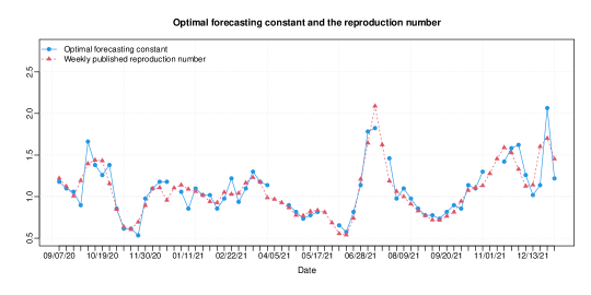
Figure 3: The optimal estimated values of the forecasting constant $C_{t,h}$, for one-week predictions i.e. $h=7$ days, are plotted along with the weekly published reproduction number $R_{t}$ that reflects the epidemiological situation at calendar time $t$.

Figure 3 shows the observed relationship between the reproduction number, which has been published weekly in France on the official website during the Covid-19 pandemic, and our optimal $C_{t,h}$ value. The value of $C_{t,h}$ that is plotted on this graph, for instance for the 7th of September 2020, is the optimal value for predicting new infections in the week ending exactly that day, and it is calculated based on the information until that day. On the other hand, according to the official website, the R-number reflects the epidemiological situation one week before notification. That is, the $R_{t}$ value that is notified on 14th of September 2020 is calculated with information until 7th of September but it is published one week later. Therefore, in Figure 3 we have plotted the $R_{t}$ series not against the date it has been published, but against the date one week earlier. Taking this into account the graph shows that each $C_{t,h}$ is very close to the published value of $R_{t}$ 7 days later. Moreover, there is a high correlation between the two indicators. As consequence we think that a reasonable good model for the $C_{t,h}$ to use for forecasting could result from a simple regression of best possible $C_{t,h}$ down on the actual and the predicted $R_{t}$. This is clearly an approach we would recommend during a developing pandemic.

7.2 Forecasting the 31th of October 2020. The Covid-19 case of France

Figure 4 gives a graphical representation of daily new infected detected from 15th of May to 31st of October 2020. The black dots give the reported daily numbers until 30 September. Our aim in this case is to forecast the number of new infections during the month of October from the information until 30th of September. Taking the value $C_{t,h}=1$ we are assuming that the immediate future will behave as the immediate past, then we assume that the rate of infection at the end of the prediction period (31-Oct) is exactly the same as it was at the end of the observation period (30-Sep). Then we obtain the dotted red line as a forecasting of the number of infected during the month of October. Taking the true number of infected reported in October (circles), we can obtain the (infeasible in practice) optimal value of $C_{t,h}$ to estimate the infection rate at the end of the prediction period. This gives the value $C_{t,h}=1.42$, what means that the rate of infection on 31st of October is $1.42$ times the value of the rate on 30th of September. Using linear interpolation we get the infection rate for the whole prediction period which allows to obtain the daily new positives in October (blue dashed line) that best fit the true values. On the graph we have also shown the case of $C_{t,h}=1$, this is, assuming that there are no changes in the behaviour of the infection rate in October with respect to what we had at the end of September. This assumption corresponds to the number of infected increasing by the trend of the red dotted line. Note that this seems to be quite wrong when we look at the true numbers (circles).

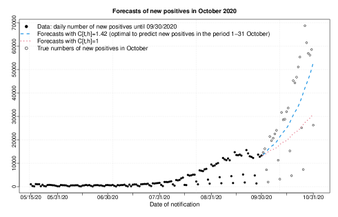
Figure 4: Number of new positives predicted in October 2020 using $C_{t,h}=1$ (red dotted line) and using the optimal value $C_{t,h}=1.42$ (blue dashed line), for $h=7$ days.

Figure 5 presents a similar study as in Figure 4 but considering the problem of predicting the number of new hospitalizations in October 2020 on the basis of historical data until 30th of September. To obtain the optimal $C_{t,h}$ value we have proceeded similarly to the previous case. We consider that the rate of infection at the end of the forecasting period is $C_{t,h}$ times the value of the infection rate we had estimated for the 30th of September. In this case we take the optimal value of $C_{t,h}$ by minimizing the error of prediction with respect to the number of hospitalized during the month of October, instead of the number of infected. Then the optimal $C_{t,h}$ leads us to a rate of infection on 31st of October that is 1.7 times the rate of infection on 30th of September (green dash-dotted line). Again, taking $C_{t,h}=1$ in this case would lead to a situation with respect to the number of new hospitalized (red dotted line) which is very far from the true situation.

To forecast the number of new hospitalized in October involves an additional step, that is, in addition to the extrapolation of the rate of infections we need to extrapolate the rate of hospitalization. Here we have assumed that the hospitalization rate at the end of the forecasting period is exactly the hospitalization rate at the end of the estimation period. Finally, we include in this graph the results obtained considering $C_{t,h}=1.42$ (blue dashed line), which is the value of the $C_{t,h}$ indicator that minimizes the error with respect to the number of infections in the forecasting period. We pay special attention to this criterion because of its relation with the popular R-number, as it has been discussed in Section 7.1.

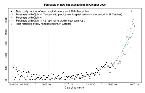
Figure 5: Number of new hospitalized predicted in October 2020 using three different values of $C_{t,h}$. The red dotted line corresponds to $C_{t,h}=1$, the green dash-dotted line $C_{t,h}=1.7$ (optimal value to predict new hospitalizations in the period 1-31 October), and the blue dashed line to $C_{t,h}=1.42$ (optimal value to predict new positives in the period 1-31 October), for $h=7$ days.

8 Conclusion

This paper has developed a new time dependent and therefore dynamic principle where the entering observations are allowed to change definitions over time as long as this change is happening in a smooth manner. This allows us to work on otherwise problematic infection and hospitalization data that were omnipresent in the recent Covid-19 pandemic. One important feature of our modelling technique is that it only relies on relatively simple available data and therefore could serve as the first model used in the beginning of a pandemic. The data definition would be simple to communicate across borders and across scientific communities and our new approach could therefore serve as a useful benchmark method when the state of the pandemic is new and confusing. While our method is applicable to other statistical modelling problems than pandemic, we will below quickly mention the relationship between our work and some of the key academic works on modelling the pandemic. We consider Quick et al (2021) to be a state-of-the-art paper published during the pandemic. They work with the development of infections and do have very interesting methodology to estimate the R-number that we also work with in this paper. Quick et al (2021) also work with simple available data, but in contradiction to our work, they build a sophisticated model of the underlying mechanism. See also Jewell (2021) and Dean and Yang (2021) for excellent discussions and intuitive explanation of Quick et al (2021). However, such a detailed micro-model does have the consequence of being limited to the problem at hand. We consider our approach to be simpler, with less bias and well fit for immediate implementation in the beginning of a pandemic. We have left the calculation of the R-number for external experts that might have prior knowledge worth incorporation. It is of course also fully aligned with our approach to fit the R-number via a regression methodology as suggested in Quick et al (2021). Mukherjee (2022) and Lin (2022) suggest that communication and general cooperation between scientific fields is a key ingredient that should be developed early on in a pandemic. The communication of our method is easy, because both input and output are easy to understand, and our method is not depending on underlying assumptions that are difficult to communicate. On the other hand, we isolate the scientific cooperation in the single number used in the forecasting (the R-number) such that experts on the R number do not need to be experts in the general scientific modelling on the problem.

There is “sister” paper to this paper, Gámiz et al. (2023), modelling how long patients stay in hospitals and whether they leave hospital alive, and adding a dynamic ratio of the relative number dying from the infection in hospital compared to those dying from the infection outside the hospital. This “sister” paper will, together with the current paper, provide a full methodology for what we call “monitoring a developing pandemic with available data”. There is an R-package under construction incorporating the methodology of both papers.

References

- Andersen et al. (1993) Andersen, P., Borgan, O., Gill, R. and Keiding, N. (1993). Statistical Models Based on Counting Processes. New York: Springer.
- Dean and Yang (2021) Dean, N., and Yang, Y. (2021). Discussion of “Regression Models for Understanding COVID-19 Epidemic Dynamics With Incomplete Data”, Journal of the American Statistical Association, 116, 1587–1590.
- Fraser (2007) Fraser, C. (2007). Estimating Individual and Household Reproduction Numbers in an Emerging Epidemic, PLoS ONE, 2(8), e758.
- Gámiz et al. (2013) Gámiz, M. L., Janys, L., Martínez-Miranda, M. D. and Nielsen, J. P. (2013). Bandwidth selection in marker dependent kernel hazard estimation, Computational Statistics & Data Analysis, 68, 155–169.
- Gámiz et al. (2016) Gámiz, M. L., Mammen, E., Martínez-Miranda, M. D. and Nielsen, J. P. (2016). Double one-sided cross-validation of local linear hazards, Journal of the Royal Statistical Society, Ser. B, 78, 755–779.
- Gámiz et al. (2022) Gámiz, M. L., Mammen, E., Martínez-Miranda, M. D. and Nielsen, J. P. (2022). Missing link survival analysis with applications to available pandemic data, Computational Statistics & Data Analysis, 169, 107405.
- Gámiz et al. (2023) Gámiz, M. L., Mammen, E., Martínez-Miranda, M. D. and Nielsen, J. P. (2023) Monitoring a developing pandemic with available data. (Submitted.)
- Garrett (2023) Garrett, A. (2023) “12 recommendations directed at improving preparedness for the UK’s statistical ecosystem. UK Covid-19 Inquiry.” Witness statement on behalf of Royal Statistical Society.
- Giudici et al. (2023) Giudici, P., Pagnottoni, P., and Spelta, A. (2023). Network self-exciting point processes to measure health impacts of COVID-19. Journal of the Royal Statistical Society Series A: Statistics in Society, qnac006.
- Goldenshluger and Koops (2019) Goldenshluger, A. and Koops, D. (2019). Nonparametric Estimation of Service Time Characteristics in Infinite-Server Queues with Nonstationary Poisson Input, Stochastic Systems, 9, 1–25.
- Heckman (1979) Heckman, J. J. (1979). Sample selection bias as a specification error, Econometrica, 47, 153–161.
- Jewell (2021) Jewell, N. P. (2021). Statistical Models for COVID-19 Incidence, Cumulative Prevalence, and , Journal of the American Statistical Association, 116, 1578–1582.
- Jiang et al. (2022) Jiang, F., Zhao, Z., and Shao, X. (2022). Modelling the COVID-19 infection trajectory: A piecewise linear quantile trend model. Journal of the Royal Statistical Society Series B: Statistical Methodology, 84(5), 1589–1607.
- Kim and Shao (2021) Kim, J. K., and Shao, J. (2021). Statistical methods for handling incomplete data. CRC press.
- Lin (2022) Lin, X. (2022). Lessons Learned from the COVID-19 Pandemic: A Statistician’s Reflection, Statistical Science, 37, 278–283.
- Little and Rubin (2019) Little, R. J., and Rubin, D. B. (2019). Statistical analysis with missing data (Vol. 793). John Wiley & Sons.
- Liu and Hu (2022) Liu, Y., and Hu, F. (2022). Balancing Unobserved Covariates With Covariate-Adaptive Randomized Experiments, Journal of the American Statistical Association., 117 (538), 875–886.
- Mammen et al. (2011) Mammen, E., Martínez-Miranda, M. D., Nielsen, J. P. and Sperlich, S. (2011). Do-validation for kernel density estimation, Journal of the American Statistical Association, 106, 651–660.
- Mammen and Müller (2023) Mammen, E. and Müller, M. (2023). Nonparametric estimation of locally stationary Hawkes processes, Bernoulli (to appear).
- Millimet and Parmeter (2022) Millimet, D. L., and Parmeter, C. F. (2022). COVID-19 severity: A new approach to quantifying global cases and deaths. Journal of the Royal Statistical Society Series A: Statistics in Society, 185(3), 1178–1215.
- Mukherjee (2022) Mukherjee, B. (2022). Being a Public Health Statistician During a Global Pandemic, Statistical Science, 37(2), 270–277.
- Nielsen (1998) Nielsen, J. P. (1998). Marker dependent kernel estimation from local linear estimation, Scandinavian Actuarial Journal, 2, 113–124.
- Nielsen and Linton (1995) Nielsen, J. P. and Linton, O. (1995). Kernel estimation in a non-parametric marker dependent hazard model, The Annals of Statistics, 23, 1735–1748.
- Park et al. (2020) Park, S. W., Bolker, B. M., Champredon, D., Earn, D. J., Li, M., Weitz, J. S., Grenfell, B.T., and Dushoff, J. (2020). Reconciling early-outbreak estimates of the basic reproductive number and its uncertainty: framework and applications to the novel coronavirus (SARS-CoV-2) outbreak. Journal of the Royal Society Interface, 17(168), 20200144.
- Pellis et al. (2022) Pellis, L., Birrell, P. J., Blake, J., Overton, C. E., Scarabel, F., Stage, H. B., Danon, L., Hall, I., House, T.A., Keeling, M.J., Read, J.M., JUNIPER Consortium, and De Angelis, D. (2022). Estimation of reproduction numbers in real time: conceptual and statistical challenges. Journal of the Royal Statistical Society Series A: Statistics in Society, 185(Supplement_1), S112–S130.
- Quick et al (2021) Quick, C., Dey, R., Lin, X. (2021). Regression Models for Understanding COVID-19 Epidemic Dynamics With Incomplete Data, Journal of the American Statistical Association, 116, 1561–1577.
- Richardson (2022) Richardson, S. (2022). Statistics in times of increasing uncertainty. Journal of the Royal Statistical Society Series A: Statistics in Society, 185(4), 1471–1496.
- Rubin (1996) Rubin,D. B. (1996). Multiple imputation after 18+ years,. Journal of the American Statistical Association, 91, 473–489.
- Samyak and Palacios (2023) Samyak, R., and Palacios, J. A. (2023). Statistical summaries of unlabelled evolutionary trees. Biometrika, asad025.
- Stokell et al. (2021) Stokell, B. G., Shah, R. D., and Tibshirani, R. J. (2021). Modelling high-dimensional categorical data using nonconvex fusion penalties. Journal of the Royal Statistical Society Series B: Statistical Methodology, 83(3), 579–611.
- Storvik et al. (2022) Storvik, G., Palomares, A. D. L., Engebretsen, S., Rø, G. Ø. I., Engø-Monsen, K., Kristoffersen, A. B., Freiesleben de Blasio, B., and Frigessi, A. (2022). A sequential Monte Carlo approach to estimate a time varying reproduction number in infectious disease models: the Covid-19 case. arXiv preprint arXiv:2201.07590.
- Zhao et al (2020) Zhao, J., Kim, H. J., Kim, H. M. (2020). New EM-type algorithms for the Heckman selection model, Computational Statistics & Data Analysis, 146, 106930.