Reach For the Spheres: Tangency-Aware Surface Reconstruction of SDFs

Abstract.

Signed distance fields (SDFs) are a widely used implicit surface representation, with broad applications in computer graphics, computer vision, and applied mathematics. To reconstruct an explicit triangle mesh surface corresponding to an SDF, traditional isosurfacing methods, such as Marching Cubes and and its variants, are typically used. However, these methods overlook fundamental properties of SDFs, resulting in reconstructions that exhibit severe oversmoothing and feature loss. To address this shortcoming, we propose a novel method based on a key insight: each SDF sample corresponds to a spherical region that must lie fully inside or outside the surface, depending on its sign, and that must be tangent to the surface at some point. Leveraging this understanding, we formulate an energy that gauges the degree of violation of tangency constraints by a proposed surface. We then employ a gradient flow that minimizes our energy, starting from an initial triangle mesh that encapsulates the surface. This algorithm yields superior reconstructions to previous methods, even with sparsely sampled SDFs. Our approach provides a more nuanced understanding of SDFs and offers significant improvements in surface reconstruction.

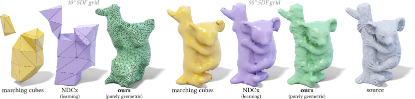
Figure 1. Reconstructing a mesh from the discrete signed distance field (SDF) of a koala (source, rightmost). By using global information from all sample points at once, our method recovers the shape even in low resolutions where methods like Marching Cubes [Lorensen and Cline, 1987] and Neural Dual Contouring (NDCx) [Chen et al., 2022a] produce very coarse shapes (left trio), and it recovers surface detail at higher resolutions that Marching Cubes and NDCx miss (middle trio). Our method is purely geometric, and does not require any training or storing of weights (unlike NDCx).

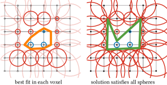
Figure 2. Reconstructing an SDF per-voxel, by finding a best fit line segment in each voxel containing both positive (red) and negative (blue) values, discards much of the available global information. Our main insight is that a solution adhering to the constraints of all spheres yields better results.

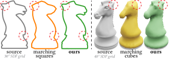
Figure 3. Using global information (not just per-voxel data), we reconstruct sharp features even at low resolutions.

1. Introduction

Signed distance fields (SDFs) are a classical implicit surface representation that finds diverse applications in computer graphics, computer vision, and applied mathematics, among other domains [Frisken et al., 2000; Sethian, 1999; Jones et al., 2006]. A continuous SDF is a scalar function $\operatorname{\phi}(\mathbf{x})$ that, given a query point $\mathbf{x}$ in $\mathbb{R}^{n}$, returns the Euclidean distance to the closest point on the surface it represents, augmented with a sign indicating whether the point is on the interior or exterior. A discrete SDF samples this function at a finite set of points in space, such as a grid, octree, or point cloud. The task we consider is the reconstruction of an explicit triangle mesh corresponding to the zero isosurface of such a discrete SDF.

Perhaps the most familiar such isosurfacing approach is Marching Cubes [Lorensen and Cline, 1987] and its variants. They use sign changes between adjacent SDF samples (e.g., along grid edges) to approximately locate the zero isosurface and apply per-cell templates and linear interpolation of the function values to fill in local patches of the surface triangulation. While effective and appropriate for general implicit surface data, these schemes ignore the unique and fundamental properties of SDFs to their detriment. Indeed, mesh reconstructions of SDF data invariably exhibit severe oversmoothing and feature loss (see Fig. 1). Approaches like dual contouring [Kobbelt et al., 2001; Ju et al., 2002] can better recover sharp features by additionally relying on surface normals. However, discrete SDFs lack the necessary gradient information and finite difference estimates give disappointing results. Is there any hope of achieving better reconstructions from the SDF data alone?

Neural Marching Cubes [Chen and Zhang, 2021] and Neural Dual Contouring [Chen et al., 2022a] have recently answered this question in the affirmative: they demonstrate better per-cell reconstructions by training on a large dataset of SDFs and using wider ($7^{3}$) stencils of SDF grid points. The quality of these results suggests that there exists some additional information implicit in the SDF data. Our objective is therefore to explicitly identify and directly exploit this overlooked geometric information, without recourse to learning approaches, and thereby achieve superior reconstructions.

The key insight underpinning our method is that (see Fig. 2) each SDF sample $\operatorname{\phi}(\mathbf{x})$ corresponds to a spherical region, centered at $\mathbf{x}$ and with radius equal to $|\operatorname{\phi}(\mathbf{x})|$. By definition, the true surface represented by the discrete SDF must be tangent to every sphere at least once while strictly containing every sphere with negative value and excluding every positive value one. Through these constraints, the SDF samples contain significantly more information about the surface than samples from a generic implicit representation would.

To fully exploit this information, we first formulate an energy that measures the degree to which a proposed surface violates the tangency constraints of the input SDF samples. We propose an algorithm that starts from a triangle mesh enclosing the surface, then ”shrinkwraps” the underlying surface via a gradient flow that minimizes our energy, interleaved with remeshing to ensure mesh quality. The fidelity of the resulting reconstructions surpasses that of prior methods, especially for sparsely sampled SDFs. Additionally, since our method has no intrinsic dependence on a grid, it is amenable to unstructured point cloud SDFs, and even incorporating new samples, where available, to improve the reconstruction.

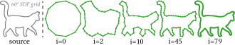
Figure 4. Our 2D flow at different iteration counts on a cat, sampled from the source mesh on the left.

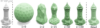
Figure 5. Our 3D flow at different iteration counts on a tower, sampled from the source mesh (left). The final version (right) has been Loop subdivided.

2. Related Work

2.1. Signed Distance Fields

SDFs have been used in countless applications spanning the computational sciences, so we highlight only a representative sample. In computer graphics they have been applied to liquid surface tracking [Foster and Fedkiw, 2001], geometric modeling [Museth et al., 2002], collision detection [Fuhrmann et al., 2003], and ray (sphere) tracing [Hart, 1996]. In traditional computer vision, uses have included image / volume segmentation [Chan and Vese, 1999] and surface reconstruction from multiview data [Faugeras and Keriven, 1998] or point clouds [Zhao et al., 2001]. In computational physics, SDFs have been applied (via the level set method) to model combustion, crystal growth, and fluid dynamics [Sethian, 1999; Osher and Fedkiw, 2003]. SDFs have also been applied to manufacturing [Brunton and Rmaileh, 2021] and robot path planning [Liu et al., 2022].

Figure 6. A green surface the sphere constraints from two SDF samples (left). The method identifies the closest point on the surface and the closest point on the sphere for each sample point $\mathbf{p}_{i}$ that makes the sphere correctly lie inside or outside the surface, as prescribed by $s_{i}$ (middle). Our flow fixes all violations until the constraints $\operatorname{\phi}(\mathbf{p}_{i},\mathcal{M})=s_{i}$ are fulfilled (right).

Figure 7. Three surfaces violating the SDF constraints in different ways, and a surface that satisfies them (left to right).

SDFs have recently seen renewed interest in the context of geometric deep learning. In particular, the DeepSDF approach [Park et al., 2019] replaces the discrete SDF with a learned continuous SDF of a shape or a space of shapes. This concept represents a subset of general neural implicit surfaces and of neural fields even more broadly [Xie et al., 2022]. Differentiable rendering with SDFs has been investigated to solve inverse problems [Bangaru et al., 2022; Vicini et al., 2022]. Since neural implicits often fail to exactly retain the signed distance property, Sharp and Jacobson [2022] propose techniques for robust geometric queries in this setting.

Despite widespread adoption of SDFs, prior techniques often view SDFs as a convenient and canonical but general implicit surface function. They may exploit the distance property in some respects, but none that we are aware of consider the additional subgrid information implied by our tangent-spheres interpretation (mentioned by Kobbelt et al. [2001]; Batty [2011]). Instead, the location of the zero isosurface is assumed to be that of the linear (or occasionally polynomial) interpolant of the SDF samples. However, away from the data points, such interpolated fields are not true SDFs.

2.2. Isosurfacing Approaches

The task of generating an explicit mesh corresponding to a given implicit surface is variously referred to as isosurfacing, polygonization, surface reconstruction, or simply meshing. There is an extensive body of literature on the topic, so we refer the reader to the survey by De Araújo et al. [2015]. There exist three broad categories of isosurfacing schemes: first, spatial subdivision schemes like Marching Cubes; second, advancing front methods, which start at a point and incrementally attach new triangles as they propagate across the surface until it is covered [Hilton et al., 1996; Sharf et al., 2006]; and third, shrinkwrap or inflation methods, which start with an initial closed surface and gradually grow it inwards or outwards to conform to the desired isosurface [Van Overveld and Wyvill, 2004; Stander and Hart, 1997; Hanocka et al., 2020]. Our method falls into the last category, which is relatively under-explored compared to the others. The work of Bukenberger and Lensch [2021] employs evolving meshes with periodic remeshing that conform to target SDFs, like our approach. They require the SDF to be resampled at every iteration of their method, while our method only requires the SDF to be evaluated on a finite set of evaluation points at the beginning (although our method can support resampling as well, see Fig. 14), and they do not use all SDF spheres’ global information.

Isosurfacing methods are often applied to SDFs, but seldom exploit the signed distance property. Indirectly, Neural Marching Cubes [Chen and Zhang, 2021] and Neural Dual Contouring [Chen et al., 2022a] represent two key exceptions. Their SDF dependence is not explicit in their algorithms, but implicitly encoded into their neural networks when trained on exact SDFs to achieve improved results compared to prior non-neural schemes. Our approach avoids any reliance on deep learning, instead making explicit use of fundamental geometric properties of SDFs.

Recently, Deep Marching Cubes (DMC) [Liao et al., 2018], MeshSDF [Remelli et al., 2020], and FlexiCubes [Shen et al., 2023] were developed to offer differentiable isosurfacing procedures. Their goal is often to incorporate isosurfacing into end-to-end deep learning pipelines for applications like shape completion, shape optimization, or single-view reconstruction. By contrast, we focus on achieving the highest quality of reconstruction of discrete SDFs. Our SDF energy has connections to the losses used in such work.

2.3. Mesh Optimization

Our algorithm uses gradient flow to optimize an energy with respect to the vertex positions of a triangle mesh, with the aim of finding a valid, tangency-aware surface reconstruction. Variational techniques in this style are ubiquitous in geometry processing applications, such as mean curvature flow and surface fairing [Desbrun et al., 1999; Kazhdan et al., 2012], mesh quality improvement [Alliez et al., 2005], Willmore flow [Crane et al., 2013], constructing coarse cages [Sacht et al., 2015], developability [Stein et al., 2018], and morphological operations [Sellán et al., 2022]. To maintain and improve mesh quality during our flow, we employ the local remeshing scheme of Botsch and Kobbelt [2004].

Our flow displaces the vertices of a mesh such that the mesh is tangent to a set of spheres centered at the SDF sample points. In a way, this can be seen as solving a reverse formulation of the medial axis computation problem. In it, one searches for maximally contained spheres tangent to a given surface, often through a combination of greedy decompositions and progressive simplifications [Li et al., 2016; Ma et al., 2012; Rebain et al., 2019].

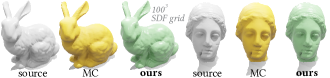
Figure 8. While our algorithm shines at low and medium resolutions, it also recovers high-frequency detail Marching Cubes misses at higher resolutions.

3. Method

Let us assume we are given access to the values $s_{1},\dots,s_{n}\in\mathbb{R}$ of the Signed Distance Function $\operatorname{\phi}$ for an unknown surface $\Omega$ sampled at $n$ points in space $\mathbf{p}_{1},\dots,\mathbf{p}_{n}\in\mathbb{R}^{3}$, $s_{i}=\operatorname{\phi}(\mathbf{p}_{i},\Omega)$. Our task will be to reconstruct a valid surface $\Omega$; i.e., one that is consistent with the SDF observations. This can be expressed as the constraints

(1) $$\operatorname{\phi}(\mathbf{p}_{i},\Omega)=s_{i}\,,\quad\forall i\in\{1,\dots,n\}\,.$$

Intuitively, one may visualize this condition by drawing a sphere $S_{i}$ of radius $|s_{i}|$ around each $\mathbf{p}_{i}$ and requiring that the surface $\Omega$ be tangent to all of them with the correct orientation (see Fig. 7).

We begin with a simple idea: turn (1) into an energy minimization problem over the space of surfaces. To this end, we define the SDF energy of a surface to be the squared difference between $s_{i}$ and the SDF value of the surface at $\mathbf{p}_{i}$:

(2) $$\operatorname{\mathcal{E}_{\operatorname{\phi}}}(\Omega)=\frac{1}{2}\sum_{i=1}^{n}\left(\operatorname{\phi}(\mathbf{p}_{i},\Omega)-s_{i}\right)^{2}\,.$$

Exploring the entire space of surfaces $\Omega$ to find one that minimizes the above energy is intractable. Instead, we propose to start from an initial surface $\Omega^{0}$ and follow the gradient flow of the SDF energy

(3) $$\frac{\partial\Omega}{\partial t}=-\nabla\operatorname{\mathcal{E}_{\operatorname{\phi}}}(\Omega)\,.$$

We refer to this as our sphere reaching flow, since it will encourage $\Omega^{t}$ to touch every $S_{i}$ at least once, while strictly containing all negative $S_{i}$ and strictly excluding all positive $S_{i}$ (see Fig. 6).

4. Discretization

We discretize the time dimension of our flow using an implicit scheme to obtain the sequence $\Omega^{0},\Omega^{1},\dots,\Omega^{T}$ of surfaces such that

(4) $$\Omega^{t}=\Omega^{t-1}-\tau\nabla\operatorname{\mathcal{E}_{\operatorname{\phi}}}\left(\Omega^{t}\right)\,$$

for some small time step $\tau$. Equivalently, given a surface $\Omega^{t-1}$, we will aim to find a new surface $\Omega^{t}$ that minimizes the energy

(5) $$\Omega^{t}=\operatorname*{argmin}_{\Omega}\frac{1}{2\tau}\left\|\Omega-\Omega^{t-1}\right\|_{2}^{2}+\operatorname{\mathcal{E}_{\operatorname{\phi}}}(\Omega)\,.$$

In order to sequentially solve this minimization problem for $t=0,\dots,T$, we will need to discretize the space of surfaces $\Omega$. We will do so by representing each surface $\Omega^{t}$ as a triangle mesh $\mathbf{\Omega}^{t}$ with vertices $\mathbf{V}^{t}$ and faces $\mathbf{F}^{t}$. (5) can then be written as

(6) $$\Omega^{t}=\operatorname*{argmin}_{\Omega}\left(\frac{1}{2\tau}\left\|\mathbf{V}-\mathbf{V}^{t-1}\right\|_{\mathbf{M}}^{2}+\operatorname{\mathcal{E}_{\operatorname{\phi}}}(\Omega)\right)\,,$$

where $\|\cdot\|_{\mathbf{M}}$ is the mass-matrix-integrated norm $\|\cdot\|^{2}_{\mathbf{M}}=\cdot^{\top}\mathbf{M}\cdot$.

Unfortunately, $\operatorname{\mathcal{E}_{\operatorname{\phi}}}(\mathbf{\Omega})$ is not convex or even continuously differentiable, which makes it difficult to minimize. To circumvent this, we first define $\mathbf{c}_{i}(\mathbf{\Omega})$ as the specific closest point on the surface $\mathbf{\Omega}$ to $\mathbf{p}_{i}$, which we can write as $\mathbf{a}_{i}({\mathbf{\Omega}})\mathbf{V}$ for some sparse vector of barycentric coordinates $\mathbf{a}_{i}({\mathbf{\Omega}})$. Then $\operatorname{\mathcal{E}_{\operatorname{\phi}}}(\mathbf{\Omega})$ becomes

(7) $$\operatorname{\mathcal{E}_{\operatorname{\phi}}}(\mathbf{\Omega})=\frac{1}{2}\sum_{i=1}^{n}\left(\operatorname{\phi}(\mathbf{p}_{i},\mathbf{c}_{i}(\mathbf{\Omega}))-s_{i}\right)^{2}$$

where we have slightly abused notation to let $\operatorname{\phi}(\mathbf{p}_{i},\mathbf{c}_{i}(\Omega))$ return the distance $\|\mathbf{p}_{i}-\mathbf{c}_{i}(\Omega)\|$ with the sign of $\operatorname{\phi}(\mathbf{p}_{i},\mathbf{\Omega})$. This modified energy penalizes distances between each closest point and the corresponding sphere’s surface. Refer to Fig. 6 for the geometric picture.

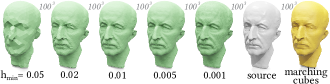
Figure 9. A critical parameter in our method is the maximum resolution, encoded in the edge-length $h_{\textrm{min}}$, which balances the under- or over-constrained nature of our optimization.

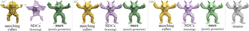
Figure 10. With no training and no network weight storage, our method consistently outperforms MC and outperforms or matches Neural DC across resolutions.

We next define $\mathbf{t}_{i}(\mathbf{\Omega})$ as the projection of $\mathbf{p}_{i}$, along the line through $\mathbf{p}_{i}(\mathbf{\Omega})$ and $\mathbf{c}_{i}(\mathbf{\Omega})$, onto the signed distance sphere $S_{i}$,

(8) $$\mathbf{t}_{i}(\mathbf{\Omega})=\mathbf{p}_{i}+\sigma_{i}|s_{i}|\frac{\mathbf{c}_{i}(\mathbf{\Omega})-\mathbf{p}_{i}}{\left\lVert\mathbf{c}_{i}(\mathbf{\Omega})-\mathbf{p}_{i}\right\rVert}\;,$$

where $\sigma_{i}$ depends on the orientation of the surface $\mathbf{\Omega}$ at $\mathbf{c}_{i}(\mathbf{\Omega})$:

• If $\mathbf{p}_{i}$ is inside/outside $\mathbf{\Omega}$ and the sign of $s_{i}$ is negative/positive, then $\sigma_{i}=1$.

• If $\mathbf{p}_{i}$ is inside/outside $\mathbf{\Omega}$ and the sign of $s_{i}$ is positive/negative, then $\sigma_{i}=-1$.

That way, if the surface were translated such that $\mathbf{c}_{i}(\mathbf{\Omega})$ coincided with $\mathbf{t}_{i}$, the SDF would be satisfied at $\mathbf{p}_{i}$. We use the mesh element’s normal vector at $\mathbf{c}_{i}(\mathbf{\Omega})$ to distinguish between inside and outside.

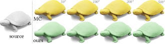
Figure 11. Our flow can be used on sparse (recovering more detail than MC) and very dense (matching MC) SDF grids.

As $\mathbf{t}_{i}(\mathbf{\Omega})$ and $\mathbf{c}_{i}(\mathbf{\Omega})$ will be equal for a valid solution, we approximate $\left(\operatorname{\phi}(\mathbf{p}_{i},\mathbf{c}_{i}(\mathbf{\Omega}))-s_{i}\right)$ by $\left\lVert\mathbf{c}_{i}(\mathbf{\Omega})-\mathbf{t}_{i}(\mathbf{\Omega}))\right\rVert$. Thus, (7) becomes

(9) $$\frac{1}{2}\sum_{i=1}^{n}\left\lVert\mathbf{c}_{i}(\mathbf{\Omega})-\mathbf{t}_{i}(\mathbf{\Omega}))\right\rVert^{2}=\frac{1}{2}\sum_{i=1}^{n}\left\lVert\mathbf{a}_{i}({\mathbf{\Omega}})\mathbf{V}-\mathbf{t}_{i}(\mathbf{\Omega})\right\rVert^{2}\,,$$

which we further simplify by fixing $\mathbf{t}_{i}(\mathbf{\Omega})$ to $\mathbf{t}_{i}\left(\mathbf{\Omega^{t-1}}\right)$.

Concatenating $\mathbf{a}_{i}$ and $\mathbf{t}_{i}$ into matrices $\mathbf{A}$ and $\mathbf{S}$, this becomes

(10) $$\frac{1}{2}\|\mathbf{A}\mathbf{V}-\mathbf{S}\|_{F}^{2}\,,$$

which we can now incorporate into (6):

(11) $$\mathbf{V}^{t}=\operatorname*{argmin}_{\mathbf{V}}\frac{1}{2\tau}\left\|\mathbf{V}-\mathbf{V}^{t-1}\right\|_{\mathbf{M}}^{2}+\frac{1}{2}\|\mathbf{A}\mathbf{V}-\mathbf{S}\|_{F}^{2}\,.$$

This quadratic optimization problem on the vertex positions $\mathbf{V}$ can be solved via the linear system

(12) $$\mathbf{Q}\mathbf{V}^{t}=\mathbf{B}$$

where

(13) $$\mathbf{Q}=\mathbf{M}+\tau\mathbf{A}^{\top}\mathbf{A}\,,\qquad\mathbf{B}=\mathbf{M}\mathbf{V}^{t-1}+\tau\mathbf{A}^{\top}\mathbf{S}\,.$$

The matrices $\mathbf{A}$, $\mathbf{M}$, and $\mathbf{Q}$ are sparse, thus the linear system can be efficiently solved using, e.g., Cholesky decomposition. A simplified step of this flow can be seen on the right of Fig. 6.

Choosing step size $\tau$.

The formulation in (12) produces a flow that, for a small enough $\tau$, will reduce the SDF energy each iteration. However, choosing $\tau$ too small can be inefficient, while $\tau$ too large will violate the linearization assumptions made in our discretization and cause flow instabilities. We use a heuristic inspired by Armijo’s condition [Nocedal and Wright, 2006] to choose the optimal step size, $\tau=\rho\operatorname{clamp}(\tau_{*},\tau_{\textrm{min}},\tau_{\textrm{max}})$, where $\rho=\frac{1}{n}$,

(14) $$\tau_{*}=-\frac{\rho(\mathbf{A}-\mathbf{S})\cdot(\mathbf{A}\mathbf{P})+0.01\lVert\mathbf{P}\rVert^{2}}{\rho\lVert\mathbf{A}\mathbf{P}\rVert^{2}},\quad\mathbf{P}=-\rho\mathbf{A}^{\top}(\mathbf{A}-\mathbf{S})\;,$$

and, by default, $\tau_{\textrm{min}}=10^{-6}$, $\tau_{\textrm{max}}=50$.

4.1. Mesh resolution and quality

As mesh vertices $\mathbf{V}$ move during our flow, mesh quality rapidly degrades, producing degeneracies, flipped and thin triangles, and self-intersections. We solve this common problem of geometric flows by remeshing with the algorithm of Botsch and Kobbelt [2004], which uses a sequence of local improvement operations. After each flow iteration, we apply a single remeshing iteration using a given target edge-length $h$ (more iterations may be used if needed). We implement this operation in an output-sensitive manner, analogous to the approach of Sellán et al. [2022], by remeshing exclusively the regions of the surface that are the closest point on $\mathbf{\Omega}$ to any of the $\mathbf{p}_{i}$ and violate the SDF value $s_{i}$ by more than a tolerance $\varepsilon$ (by default, $5\cdot 10^{-3}$ for 2D and $10^{-2}$ for 3D).

Both our flow and our remeshing operations preserve the intrinsic shape’s topology. This restriction helps us avoid some of the most catastrophic failures of existing methods like Marching Cubes, which can produce wrongly disconnected mesh components at low resolutions (see Figs. 1, 10). At the same time, it means that our starting surface mesh $\Omega^{0}$ needs to agree with the topology of the surface to be reconstructed.

Careful consideration must also be given to the mesh resolution during our flow, as encoded in the remesher’s target edge-length, $h$. As shown in Fig. 3, our flow is capable of recovering much more faithful surface detail than existing grid-based methods. Thus, we naturally wish to provide it with enough degrees of freedom (sufficiently low target edge-length $h$) to accurately represent the surface. At the same time, too many mesh vertices will make our flow iterations costly and the sphere reaching problem underconstrained.

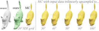
Figure 12. Our algorithm’s full exploitation of all the SDF input data means its improved performance against Marching Cubes is preserved even if one artificially upsamples the SDF input before using MC.

Ideally, then, we wish our flow to produce the lowest possible resolution mesh that can explain all SDF samples. We will achieve this by starting from a very high value of $h$ and running our flow until convergence, as identified by the energy’s failure to decrease further than by a tolerance ($10^{-3}\varepsilon$) in the past 10 iterations, to obtain a coarse approximation of the surface (see inset). We will then halve $h$ and run our flow again, noting that our output-sensitive remesher will only refine the regions of the shape that are contributing to the energy (i.e., those that need the additional resolution). We repeat this process until a minimum $h_{min}$ is reached, by default set to be the average distance between SDF samples $\mathbf{p}_{i}$. Once $h_{\min}$ is reached, we run our flow until the energy has not decreased by more than $10^{-3}\varepsilon$ in the past $100$ iterations.

Batching.

In practice, our algorithm’s computational cost is dominated by the assembly of $\mathbf{A}$, which requires $n$ signed distance and closest point queries between each sphere origin and the current reconstruction mesh. Even though we manage to resolve each query in logarithmic time by assembling and using a bounding volume hierarchy, computing all $n$ queries can be costly. Thus, for large values of $n$ (e.g., $n>50^{3}$), we propose using randomly chosen batches of spheres at each iteration. Empirically, we note that interior spheres are more critical to our flow’s stability; therefore, we only batch exterior spheres. By default, we make the batch size $\min(n,20000)$.

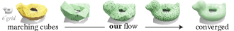
Figure 13. Our flow is not limited to genus zero shapes, but the topology of the initial surface must match the reconstruction’s. Marching Cubes may provide a good starting surface in these non-genus-zero cases.

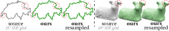
Figure 14. We can further improve the reconstruction quality on coarse grids by adding just a few SDF samples after the flow has converged, due to the gridless nature of our method.

5. Results & Experiments

Implementation details.

We implemented our algorithm in Python using Gpytoolbox [Sellán and Stein, 2023] for common geometry processing subroutines including our flow’s remesher as well as the Marching Cubes reconstruction [Lorensen and Cline, 1987] used in our comparisons. Our comparisons to Neural Dual Contouring [Chen et al., 2022a] use the authors’ publicly available implementation, including following their preprocessing instructions. We report timings on a 20-Core M1 Ultra Mac Studio with 128GB RAM. We rendered our figures in Blender, using BlenderToolbox [Liu, 2023].

Our method’s complexity is determined by three algorithmic steps that must be executed at each flow iteration. First, the signed distances from each $\mathbf{p}_{i}$ to the current mesh are computed with a complexity of $\mathcal{O}((b+m)\log(m))$ (where $m$ is the number of current mesh vertices and $b$ is the batch size). Secondly, the linear system in Eq. (12) adds an $\mathcal{O}(m^{1+f})$ term, where $f$ accounts for the sparse system solve (we cannot take advantage of precomputation as the mesh changes in every iteration). Finally, our remeshing step adds an $\mathcal{O}(\tilde{m})$ term, where $\tilde{m}<m$ is the size of the active region of the current mesh. In the limit, this means each flow iteration will be asymptotically dominated by $\max(b\log(m),m^{1+f})$; in practice, we find this to be the case except for very low values of $m$ and $b$, where the constant factors in the remesher complexity dominate.

Our input shapes are scaled to fit the box $[-\frac{1}{2},\frac{1}{2}]^{n}$, and our SDF grids are constructed in $[-1,1]^{n}$. We use default parameters, unless otherwise specified in the supplemental material. Unless otherwise specified, we initialize our examples with a unit icosahedral sphere, but our flow can handle other initializations (Fig. 13).

Grid size	Hdf MC	Hdf NDCx	Hdf Ours	Chr MC	Chr NDCx	Chr Ours	$\operatorname{\mathcal{E}_{\operatorname{\phi}}}$ MC	$\operatorname{\mathcal{E}_{\operatorname{\phi}}}$ NDCx	$\operatorname{\mathcal{E}_{\operatorname{\phi}}}$ Ours	Time Ours
$6^{3}$	0.3351	0.2597	0.1236	0.1918	0.1135	0.0569	31.4645	10.2969	0.1091	1.1214
$10^{3}$	0.2518	0.1954	0.0846	0.1053	0.0662	0.0343	13.8933	6.2637	0.1152	1.2686
$20^{3}$	0.1486	0.1163	0.0631	0.0465	0.0311	0.0210	4.7667	2.8065	0.1377	4.7881
$30^{3}$	0.0756	0.0494	0.0396	0.0206	0.0127	0.0118	0.6125	0.1451	0.0280	6.0939
$40^{3}$	0.0581	0.0366	0.0417	0.0143	0.0089	0.0100	0.3933	0.0910	0.0135	6.6929
$50^{3}$	0.0501	0.0360	0.0253	0.0107	0.0077	0.0074	0.2451	0.1042	0.0050	9.4438

Table 1. Across a diverse set of examples and resolutions, our flow exhibits lower Hausdorff (”Hdf”), Chamfer (”Chr”) and SDF ($\operatorname{\mathcal{E}_{\operatorname{\phi}}}$) errors than Marching Cubes, while surpassing or matching data-driven approaches like Neural Dual Contouring. Time given in seconds. Data averaged over Table 2 (supplemental).

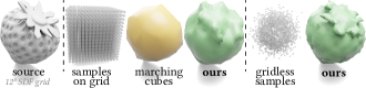
Figure 15. SDF sampled from the same source on a grid and with the same number of samples on a noisy point cloud of the source. Alternate sampling strategies unavailable to grid-based methods allow us to recover more information with the same number of SDF samples.

5.1. Comparisons

The sole input to our algorithm is a set of query points $\mathbf{p}_{i}$ and corresponding SDF values $s_{i}$. In the specific case where these samples are placed on a structured grid, this input matches that of the timeless reconstruction algorithm Marching Cubes [Lorensen and Cline, 1987]. By allowing for the training on a vast dataset and the storing of a large number of network weights, recent advances like Neural Dual Contouring [Chen et al., 2022a] have been shown to outperform most other reconstruction algorithms.

Qualitative comparisons.

Throughout the paper, we qualitatively show our algorithm’s improved performance against Marching Cubes (MC). At low resolutions, MC often produces little more than disconnected “blobs”, often missing entire regions of the shape (see Figs. 1, 10). By contrast, our method shines at these resolutions, where exploiting all the global information provided by the SDF samples can recover features completely absent from the MC reconstruction (see Figs. 3 and 15), an advantage that is preserved even if the data is upsampled artificially to denser grids (see Fig. 12). Even at higher resolutions, our global SDF-aware reconstruction captures significantly more detail (see Figs. 8, 9 and 11).

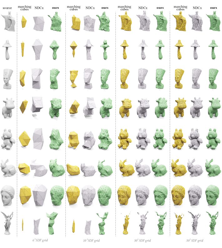
Figure 21. Our algorithm strikingly outperforms Marching Cubes and Neural Dual Contouring (NDCx) at low and medium resolutions.

In Figs. 1, 10, and 21, we additionally compare our algorithm’s effectiveness with Neural Dual Contouring [Chen et al., 2022a]. To make the comparison as generous as possible, we used the highest performing version of the authors’ publicly available trained models [Chen et al., 2022b], NDCx, which combines their network with elements of their previous work’s learned model [Chen and Zhang, 2021]. Even though their data-driven approach manages to outperform Marching Cubes in almost all our tests, we qualitatively find that our purely geometric algorithm consistently outperforms both at low and medium resolutions despite requiring no training.

Quantitative comparisons.

Inspired by the evaluations in the work by Chen et al. [2022a], we also compare our algorithm’s performance quantitatively. In Fig. 21, we run our algorithm using its default parameters as well as Marching Cubes and NDCx on shapes from a diverse set of origins whose SDFs have been sampled at different resolutions. In our supplemental material, we attach a table comparing the Hausdorff distance to the ground truth mesh as well as Chamfer distance and our own SDF energy $\operatorname{\mathcal{E}_{\operatorname{\phi}}}$, while Table 1 shows the average values for each resolution. While placing fewer requirements on the input (any set of points $\mathbf{p}_{i}$ versus a structured grid), our algorithm consistently outperforms Marching Cubes across the board, often by several integer factors. While requiring no training, our algorithm surpasses NDCx at low resolutions and remains competitive at medium and higher resolutions. We note that MC requires between $20^{3}$ and $30^{3}$ SDF grid samples to match the accuracy of our algorithm at the lowest of resolutions ($6^{3}$ grid). Thus, our algorithm reduces memory storage requirements for equal surface accuracy by a factor of between $37$ and $125$.

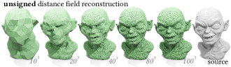
Figure 16. By relaxing the constraints in our method, our flow can be seamlessly applied to unsigned distance fields at diverse resolutions.

5.2. Parameters

A number of parameters affect our method’s ability to extract all information from its SDF input. Among these, the most crucial is the minimum mesh edge-length $h_{\min}$. Choosing $h_{\min}$ too high can cause the method to miss information available in the SDF samples. A very small $h_{\min}$ can negatively affect performance, and also underconstrain the problem, leading to (completely valid) solutions that have high-frequency noise. Our remeshing procedure contains a regularization step that combats this noise, but does not completely obviate it. Empirically, we find that setting $h_{\min}$ to be the average closest-distance between samples $\mathbf{p}_{i}$ (i.e., the gridless analogue of the grid edge-length) is a useful heuristic, whose reliability we show across resolutions in Fig. 21, Table 1 and the supplemental.

5.3. SDF sampling

While many algorithms rely on SDF samples to be located on a structured (regular or not) grid, our method is completely agnostic to the position of the samples $\mathbf{p}_{i}$. We can take advantage of this in multiple ways. For example, we can run our algorithm, unchanged, on SDF data sampled on fully unstructured point clouds, exploiting prior information (Fig. 15). In settings where the source SDF function is available to be queried, we can add more samples $(\mathbf{p}_{i},s_{i})$ after our method has converged, and run it from the previous result (Fig. 14) to incrementally improve the reconstruction. Our heuristic for adding samples is to generate $m_{\textrm{trial}}$ samples on $\mathbf{\Omega}$, randomly displace them in the normal direction by a normal distribution scaled by $0.05$, and select the $m_{\textrm{new}}$ samples farthest away from the surface of any SDF sphere (but at most one per mesh element). By default, $m_{\textrm{new}}=2\sqrt{n}$ in 2D, $m_{\textrm{new}}=2\sqrt[3]{n}$ in 3D, and $m_{\textrm{trial}}=50m_{\textrm{new}}$.

5.4. Beyond SDFs

Signed Distance Fields are a powerful representation that we have shown can be exploited to obtain a surprisingly large amount of information about a given object. Often, however, computing exact SDFs can be costly or impracticable, forcing one to relax some of the assumptions in the traditional SDF definition.

Consider the case of unsigned distance fields, which lack the inside-outside information contained in the sign of traditional SDFs. As shown in Fig. 16, our flow can very easily be employed to reconstruct meshes from these functions, merely by always making $\sigma_{i}=1$ in (8). Intuitively, this means we move the surface towards the closer of the sphere’s two possible tangent points, $\mathbf{t}_{i}$.

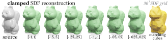
Figure 17. Clamped or truncated SDFs discard information our method needs to capture the shape’s detail, but our method degrades gracefully and still outperforms Marching Cubes even for aggressive clamping parameters.

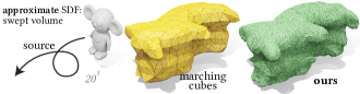
Figure 18. A swept volume SDF is accurate only outside the object. Inside, it is only a bound on distance. By relaxing its assumptions, we can use our method for swept volume reconstruction.

Another relaxation of SDFs are clamped, truncated, or narrow band SDFs, that take a constant value at spatial positions “sufficiently far” from the surface. This is a common representation in highly performant modelling applications and, more recently, in machine learning models when one wants to focus learning near the object’s surface (see, e.g., [Park et al., 2019]). Generalizing our algorithm to these representations is conceptually simple: for a given clamp value $\sigma_{c}$, we allow the tangency requirement (but not the intersection-free one) to be violated for those spheres with radii larger than $\sigma_{c}$. In practice, this amounts to zeroing out the $i$-th row of $\mathbf{A}$ if $|\phi(\mathbf{p}_{i},\Omega^{t})|>|s_{i}|>\sigma_{c}$. Our algorithm relies on faraway spheres to provide additional information about the reconstruction; therefore, using a clamped SDF necessarily results in a progressive loss of detail (see Fig. 17).

Yet another common SDF-based representation is formed by instead providing bounds on the true shape’s signed distance (these are referred to as conservative SDFs by Takikawa et al. [2022]). Such SDFs appear naturally as the output of Boolean operations on signed distance functions. A recently studied example of this are swept volumes, which can be represented by taking the minimum of the SDF of an object along a trajectory; however, this representation is only an exact SDF outside the volume, while only a bound inside. As we show in Fig. 18, all that is needed to apply our flow to swept volume reconstruction is to relax the tangency constraint of the negative-sign spheres only. In practice, this amounts to zeroing the $i$-th row of $A$ if $|\phi(\mathbf{p}_{i},\Omega^{t})|>|s_{i}|$ and $s_{i}<0$. We believe this to be a promising application of our work, as swept volume approximate SDFs are often extremely costly to query [Sellán et al., 2021].

6. Discussion and Conclusions

We have leveraged our new tangent-spheres interpretation to develop an effective isosurfacing method, called Reach for the Spheres, that exploits the full representational power of SDFs. Using only geometric information present in a standard discrete SDF, we are able to recover noticeably more detail than previous general-purpose isosurfacing schemes. Our method especially shines on low-resolution SDF grids, where it is able to exploit every last bit of information that other methods might miss, and it can match traditional methods for high resolutions. By releasing our method to the Graphics community, we hope to renew interest in lightweight, low-resolution SDF representations and enable novel, scalable applications.

Our method is not yet robust to self-intersections, nor does it support topology changes, as needed to straightforwardly handle difficult multi-component or nonzero genus shapes. Thus, as a limitation, our method can exhibit self-intersection and pinching effects due to singularities in the discrete flow (Fig. 19). Our algorithm’s current inability to handle these singularities also limits its efficacy on noisy SDF data (see Fig. 20). We are optimistic that existing mesh-based fluid simulation surface tracking techniques [Wojtan et al., 2011] can help overcome these restrictions.

Furthermore, a surface that perfectly satisfies a given discrete SDF can often still have significant flexibility at the finer scales; an exciting direction is to incorporate specific priors for particular applications, via additional regularization or data-driven approaches. There is also ample room to improve the performance of our method, by using more elaborate methods for closest point computations, solving linear equations, and remeshing.

Beyond surface reconstruction, a vast array of other graphics techniques rely on discrete SDFs across simulation, geometry processing, and rendering. We look forward to exploring whether incorporating the tangent-spheres perspective can yield comparable improvements for these applications as well.

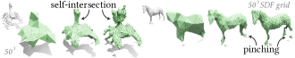
Figure 19. Like many geometric flows, our algorithm can occasionally produce singularities, corresponding to attempts to dynamically change topology.

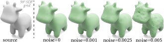
Figure 20. Adding Gaussian noise to the SDF input values, with increasing standard deviation. For small values, our flow degenerates gracefully. At a standard deviation of 0.005 (i.e., 0.5% of the shape’s bounding box length), our flow hits a singularity before the stopping criterion is reached.

Supplemental Material

Parameters

In this section we list $h_{\textrm{min}}$ and non-default parameters used in this article.

Fig. 1.

$h_{\textrm{min}}=0.02$ for grid size $10$. $h_{\textrm{min}}=0.01$ for grid size $50$. $\varepsilon=10^{-4}$. $3$ remesh iterations.

Fig. 3.

$h_{\mathrm{min}}=0.03$. $t_{\mathrm{max}}=10$ in 3D.

Fig. 4.

$h_{\mathrm{min}}=0.01$.

Fig. 5.

$h_{\mathrm{min}}=0.02$. Batching turned off.

Fig. 8.

$h_{\textrm{min}}=0.008$.

Fig. 10.

Left to right: $h_{\min}=0.05$, $0.02$ and $0.008$.

Fig. 11.

For grid size $n^{3}$, $h_{\mathrm{min}}=\frac{2}{n}$, and $\varepsilon=\frac{10^{-2}}{n}$.

Fig. 14.

$h_{\mathrm{min}}=0.035$ in 2D; $h_{\mathrm{min}}=0.04$ in 3D.

Fig. 15.

$h_{\mathrm{min}}=0.06$. $\varepsilon=10^{-3}$

Fig. 20.

$h_{\mathrm{min}}=0.015$.

Detailed Quantitive Evaluation Data

Table 2 contains the detailed results of our quantitative evaluations for the SDF reconstruction problem on a variety of shapes, comparing our method with Marching Cubes and NDCx.

Shape	$n$	Hdf MC	Hdf NDCx	Hdf Ours	Chr MC	Chr NDCx	Chr Ours	$\operatorname{\mathcal{E}_{\operatorname{\phi}}}$ MC	$\operatorname{\mathcal{E}_{\operatorname{\phi}}}$ NDCx	$\operatorname{\mathcal{E}_{\operatorname{\phi}}}$ Ours	Time Ours
mushroom	6	0.1952	0.1489	0.1417	0.1274	0.1103	0.0753	11.7905	1.1676	0.0519	0.5147
mushroom	10	0.1221	0.0819	0.1023	0.0715	0.0456	0.0420	3.9187	0.4795	0.0455	1.1983
mushroom	20	0.0611	0.0485	0.0606	0.0345	0.0197	0.0200	0.5752	0.1567	0.0519	6.0584
mushroom	30	0.0546	0.0233	0.0407	0.0215	0.0114	0.0116	0.3133	0.0758	0.0150	3.9053
mushroom	40	0.0532	0.0217	0.0238	0.0165	0.0077	0.0077	0.2285	0.0286	0.0092	4.1968
mushroom	50	0.0382	0.0186	0.0188	0.0120	0.0065	0.0062	0.1012	0.0128	0.0038	7.1066
nefertiti	6	0.2007	0.1296	0.0988	0.1384	0.0671	0.0462	11.9997	0.6109	0.0520	1.8593
nefertiti	10	0.1826	0.0760	0.0645	0.0976	0.0379	0.0188	5.1541	0.3250	0.0427	1.6463
nefertiti	20	0.0744	0.0419	0.0381	0.0304	0.0146	0.0142	0.9196	0.0742	0.0416	6.6072
nefertiti	30	0.0406	0.0382	0.0286	0.0144	0.0080	0.0086	0.2235	0.0414	0.0145	10.2500
nefertiti	40	0.0382	0.0287	0.0246	0.0119	0.0063	0.0069	0.1655	0.0190	0.0100	6.4140
nefertiti	50	0.0341	0.0316	0.0264	0.0076	0.0056	0.0059	0.0459	0.0128	0.0032	11.1034
bunny	6	0.2947	0.1669	0.1769	0.1997	0.0938	0.0626	15.2121	1.9051	0.0438	0.9502
bunny	10	0.4295	0.4051	0.0860	0.1199	0.0982	0.0332	16.6344	11.3773	0.0685	1.3017
bunny	20	0.1975	0.1348	0.0612	0.0453	0.0271	0.0182	3.6855	1.0939	0.0527	4.2061
bunny	30	0.0580	0.0383	0.0397	0.0158	0.0110	0.0097	0.2503	0.0349	0.0226	8.9931
bunny	40	0.0638	0.0273	0.0351	0.0131	0.0086	0.0080	0.1889	0.0196	0.0097	10.1580
bunny	50	0.0487	0.0309	0.0219	0.0090	0.0069	0.0063	0.0789	0.0096	0.0035	14.7060
argonath	6	0.3763	0.2707	0.1146	0.2341	0.0827	0.0393	42.1481	6.2328	0.1402	0.7281
argonath	10	0.3271	0.2104	0.0751	0.0919	0.0548	0.0314	12.6527	5.5259	0.2200	0.9053
argonath	20	0.1707	0.1538	0.0486	0.0482	0.0334	0.0214	4.4039	1.7451	0.0794	5.2204
argonath	30	0.0953	0.0401	0.0320	0.0197	0.0120	0.0119	0.8446	0.1481	0.0318	4.0973
argonath	40	0.0513	0.0282	0.0303	0.0149	0.0084	0.0089	0.3563	0.0245	0.0139	6.2986
argonath	50	0.0443	0.0237	0.0274	0.0097	0.0065	0.0067	0.2083	0.0196	0.0067	8.0372
lucy	6	0.4025	0.3718	0.0974	0.1601	0.1128	0.0549	45.0055	19.7607	0.5921	0.3424
lucy	10	0.4490	0.4405	0.1046	0.1599	0.1356	0.0499	44.8871	29.1435	0.4019	0.7341
lucy	20	0.4054	0.3611	0.0937	0.1161	0.0943	0.0349	27.0360	20.5396	0.8438	4.6527
lucy	30	0.1243	0.1190	0.0757	0.0358	0.0251	0.0232	1.5015	0.4685	0.0952	4.6289
lucy	40	0.1162	0.1166	0.0534	0.0258	0.0183	0.0164	1.3426	0.4506	0.0531	6.1530
lucy	50	0.1409	0.1176	0.0380	0.0227	0.0178	0.0140	1.4041	0.8705	0.0117	5.4008
igea	6	0.1716	0.1026	0.0602	0.1192	0.0561	0.0218	4.3137	1.1548	0.0158	1.2822
igea	10	0.1078	0.0727	0.0470	0.0554	0.0294	0.0164	1.3410	0.3004	0.0119	2.3998
igea	20	0.0653	0.0421	0.0569	0.0203	0.0149	0.0143	0.2639	0.0748	0.0151	4.3184
igea	30	0.0386	0.0276	0.0292	0.0116	0.0093	0.0087	0.0687	0.0237	0.0047	6.2384
igea	40	0.0296	0.0184	0.0237	0.0089	0.0071	0.0074	0.0368	0.0061	0.0023	7.4121
igea	50	0.0259	0.0136	0.0207	0.0075	0.0065	0.0067	0.0222	0.0049	0.0017	9.0712
armadillo	6	0.5501	0.4145	0.1573	0.2729	0.1810	0.0911	78.0223	33.4996	0.0651	1.0500
armadillo	10	0.3669	0.2590	0.1167	0.1816	0.1028	0.0490	35.4634	11.6023	0.1679	1.0748
armadillo	20	0.1925	0.1766	0.0495	0.0658	0.0488	0.0209	6.9130	3.7000	0.0893	4.1866
armadillo	30	0.1382	0.0931	0.0396	0.0283	0.0189	0.0129	1.4777	0.4933	0.0418	5.0136
armadillo	40	0.1067	0.0624	0.1335	0.0191	0.0116	0.0221	1.2729	0.2819	0.0149	2.7483
armadillo	50	0.0770	0.0573	0.0302	0.0125	0.0091	0.0085	0.3559	0.0883	0.0083	8.8009
teddy	6	0.2284	0.1726	0.1407	0.1369	0.0836	0.0587	11.9344	2.0409	0.0347	1.7151
teddy	10	0.1692	0.1615	0.1039	0.0922	0.0655	0.0418	4.4468	1.6534	0.0409	1.2807
teddy	20	0.1280	0.1122	0.0821	0.0363	0.0262	0.0255	1.0904	0.4025	0.0473	4.4172
teddy	30	0.0480	0.0279	0.0353	0.0177	0.0115	0.0113	0.1661	0.0561	0.0144	7.2587
teddy	40	0.0410	0.0232	0.0473	0.0117	0.0083	0.0090	0.0641	0.0361	0.0067	5.6651
teddy	50	0.0343	0.0266	0.0275	0.0092	0.0068	0.0070	0.0284	0.0093	0.0031	8.0650
spot	6	0.2901	0.3463	0.1325	0.2069	0.1743	0.0619	24.3347	11.6865	0.0313	1.2620
spot	10	0.2188	0.1574	0.0654	0.1177	0.0621	0.0291	10.7422	2.1484	0.0498	1.0666
spot	20	0.0932	0.0451	0.0508	0.0313	0.0176	0.0189	1.0994	0.2004	0.0602	4.6396
spot	30	0.0654	0.0474	0.0465	0.0158	0.0101	0.0092	0.2841	0.0871	0.0135	4.3807
spot	40	0.0320	0.0209	0.0231	0.0095	0.0069	0.0063	0.0520	0.0293	0.0043	7.5936
spot	50	0.0251	0.0264	0.0180	0.0077	0.0059	0.0056	0.0302	0.0112	0.0021	11.0150

Table 2. Quantitative Evaluation Data

References

- [1]
- Aim Shape repository [2011] Aim Shape repository. 2011. Squirrel. https://www.thingiverse.com/thing:11705.
- Al-Badri and Nelles [2016] Nora Al-Badri and Jan Nikolai Nelles. 2016. Nefertiti. https://github.com/odedstein/meshes/tree/master/objects/nefertiti.
- Alliez et al. [2005] Pierre Alliez, David Cohen-Steiner, Mariette Yvinec, and Mathieu Desbrun. 2005. Variational Tetrahedral Meshing. In ACM SIGGRAPH 2005 Papers. 617–625. https://doi.org/10.1145/1186822.1073238
- Bangaru et al. [2022] Sai Praveen Bangaru, Michaël Gharbi, Fujun Luan, Tzu-Mao Li, Kalyan Sunkavalli, Milos Hasan, Sai Bi, Zexiang Xu, Gilbert Bernstein, and Fredo Durand. 2022. Differentiable rendering of neural SDFs through reparameterization. In SIGGRAPH Asia 2022 Conference Papers. Article 5, 9 pages. https://doi.org/10.1145/3550469.3555397
- Batty [2011] Christopher Batty. 2011. Problem: Reconstructing meshes with sharp features from signed distance data. Personal website, https://web.archive.org/web/20111112202136/http://www.cs.columbia.edu/~batty/misc/levelset_meshing/level_set_reconstruction.html.
- billyd [2016] billyd. 2016. Cat Stretch. https://www.thingiverse.com/thing:1565405.
- Botsch and Kobbelt [2004] Mario Botsch and Leif Kobbelt. 2004. A remeshing approach to multiresolution modeling. In Proceedings of the 2004 Eurographics/ACM SIGGRAPH symposium on Geometry processing. 185–192. https://doi.org/10.1145/1057432.1057457
- Brunton and Rmaileh [2021] Alan Brunton and Lubna Abu Rmaileh. 2021. Displaced Signed Distance Fields for Additive Manufacturing. ACM Trans. Graph. 40, 4, Article 179 (2021), 13 pages. https://doi.org/10.1145/3450626.3459827
- Bukenberger and Lensch [2021] Dennis R. Bukenberger and Hendrik P. A. Lensch. 2021. Be Water My Friend: Mesh Assimilation. Vis. Comput. 37, 9–11 (2021), 2725–2739. https://doi.org/10.1007/s00371-021-02183-6
- Chan and Vese [1999] Tony Chan and Luminita Vese. 1999. An active contour model without edges. In Scale-Space Theories in Computer Vision. Springer, 141–151. https://doi.org/10.1007/3-540-48236-9_13
- Chen et al. [2022a] Zhiqin Chen, Andrea Tagliasacchi, Thomas Funkhouser, and Hao Zhang. 2022a. Neural dual contouring. ACM Trans. Graph. 41, 4, Article 104 (2022), 13 pages. https://doi.org/10.1145/3528223.3530108
- Chen et al. [2022b] Zhiqin Chen, Andrea Tagliasacchi, Thomas Funkhouser, and Hao Zhang. 2022b. Neural dual contouring – GitHub repository. https://github.com/czq142857/NDC.
- Chen and Zhang [2021] Zhiqin Chen and Hao Zhang. 2021. Neural marching cubes. ACM Trans. Graph. 40, 6, Article 251 (2021), 15 pages. https://doi.org/10.1145/3478513.3480518
- Cornelis Brouwers [2014] Cornelis Brouwers. 2014. Teddy. https://www.thingiverse.com/techkey/designs.
- cosmicblobs [2021] cosmicblobs. 2021. cheburashka. accessed at libigl https://github.com/libigl/libigl-tutorial-data.
- Crane [2013a] Keenan Crane. 2013a. bob. https://www.cs.cmu.edu/~kmcrane/Projects/ModelRepository/.
- Crane [2013b] Keenan Crane. 2013b. Spot. https://www.cs.cmu.edu/~kmcrane/Projects/ModelRepository/.
- Crane et al. [2013] Keenan Crane, Ulrich Pinkall, and Peter Schröder. 2013. Robust fairing via conformal curvature flow. ACM Trans. Graph. 32, 4, Article 61 (2013), 10 pages. https://doi.org/10.1145/2461912.2461986
- Cyberware Inc. [2023a] Cyberware Inc. 2023a. Horse. https://github.com/alecjacobson/common-3d-test-models/blob/master/data/horse.obj (year denotes online access).
- Cyberware Inc. [2023b] Cyberware Inc. 2023b. Igea. https://github.com/alecjacobson/common-3d-test-models/blob/master/data/igea.obj (year denotes online access).
- De Araújo et al. [2015] Bruno Rodrigues De Araújo, Daniel S Lopes, Pauline Jepp, Joaquim A Jorge, and Brian Wyvill. 2015. A survey on implicit surface polygonization. ACM Computing Surveys (CSUR) 47, 4, Article 60 (2015), 39 pages. https://doi.org/10.1145/2732197
- Desbrun et al. [1999] Mathieu Desbrun, Mark Meyer, Peter Schröder, and Alan H Barr. 1999. Implicit fairing of irregular meshes using diffusion and curvature flow. In Proceedings of the 26th annual conference on Computer graphics and interactive techniques. 317–324. https://doi.org/10.1145/311535.311576
- Faugeras and Keriven [1998] O. Faugeras and R. Keriven. 1998. Variational principles, surface evolution, PDEs, level set methods, and the stereo problem. IEEE Transactions on Image Processing 7, 3 (1998), 336–344. https://doi.org/10.1109/83.661183
- Foster and Fedkiw [2001] Nick Foster and Ronald Fedkiw. 2001. Practical animation of liquids. In Proceedings of the 28th annual conference on Computer graphics and interactive techniques. 23–30. https://doi.org/10.1145/383259.383261
- Frisken et al. [2000] Sarah F Frisken, Ronald N Perry, Alyn P Rockwood, and Thouis R Jones. 2000. Adaptively sampled distance fields: A general representation of shape for computer graphics. In Proceedings of the 27th annual conference on Computer graphics and interactive techniques. 249–254. https://doi.org/10.1145/344779.344899
- Fuhrmann et al. [2003] Arnulph Fuhrmann, Gerrit Sobotka, and Clemens Groß. 2003. Distance fields for rapid collision detection in physically based modeling. In Proceedings of GraphiCon, Vol. 2003. 58–65.
- GSC_Nakamura [2013] GSC_Nakamura. 2013. Strawberry. https://www.thingiverse.com/thing:153548.
- Hanocka et al. [2020] Rana Hanocka, Gal Metzer, Raja Giryes, and Daniel Cohen-Or. 2020. Point2Mesh: A Self-Prior for Deformable Meshes. ACM Trans. Graph. 39, 4, Article 126 (2020). https://doi.org/10.1145/3386569.3392415
- Hart [1996] John C Hart. 1996. Sphere tracing: A geometric method for the antialiased ray tracing of implicit surfaces. The Visual Computer 12, 10 (1996), 527–545. https://doi.org/10.1007/s003710050084
- Hilton et al. [1996] Adrian Hilton, Andrew J Stoddart, John Illingworth, and Terry Windeatt. 1996. Marching triangles: range image fusion for complex object modelling. In Proceedings of 3rd IEEE international conference on image processing, Vol. 2. IEEE, 381–384. https://doi.org/10.1109/ICIP.1996.560840
- Holinaty [2020] Josh Holinaty. 2020. Mushroom. https://github.com/odedstein/meshes/tree/master/objects/mushroom.
- jansentee3d [2018] jansentee3d. 2018. Dragon Tower. https://www.thingiverse.com/thing:3155868.
- Jones et al. [2006] Mark W Jones, J Andreas Baerentzen, and Milos Sramek. 2006. 3D distance fields: A survey of techniques and applications. IEEE Transactions on visualization and Computer Graphics 12, 4 (2006), 581–599. https://doi.org/10.1109/TVCG.2006.56
- Ju et al. [2002] Tao Ju, Frank Losasso, Scott Schaefer, and Joe Warren. 2002. Dual contouring of hermite data. In Proceedings of the 29th annual conference on Computer graphics and interactive techniques. 339–346. https://doi.org/10.1145/566570.566586
- Kazhdan et al. [2012] Michael Kazhdan, Jake Solomon, and Mirela Ben-Chen. 2012. Can Mean-Curvature Flow be Modified to be Non-singular? Computer Graphics Forum 31, 5 (2012), 1745–1754. https://doi.org/10.1111/j.1467-8659.2012.03179.x
- Kobbelt et al. [2001] Leif P Kobbelt, Mario Botsch, Ulrich Schwanecke, and Hans-Peter Seidel. 2001. Feature sensitive surface extraction from volume data. In Proceedings of the 28th annual conference on Computer graphics and interactive techniques. 57–66. https://doi.org/10.1145/383259.383265
- Li et al. [2016] Pan Li, Bin Wang, Feng Sun, Xiaohu Guo, Caiming Zhang, and Wenping Wang. 2016. Q-mat: Computing medial axis transform by quadratic error minimization. ACM Trans. Graph. 35, 1, Article 8 (2016), 16 pages. https://doi.org/10.1145/2753755
- Liao et al. [2018] Yiyi Liao, Simon Donne, and Andreas Geiger. 2018. Deep marching cubes: Learning explicit surface representations. In Proceedings of the IEEE Conference on Computer Vision and Pattern Recognition. 2916–2925. https://doi.org/10.1109/CVPR.2018.00308
- Liu [2023] Hsueh-Ti Derek Liu. 2023. BlenderToolbox. https://github.com/HTDerekLiu/BlenderToolbox.
- Liu et al. [2022] Puze Liu, Kuo Zhang, Davide Tateo, Snehal Jauhri, Jan Peters, and Georgia Chalvatzaki. 2022. Regularized Deep Signed Distance Fields for Reactive Motion Generation. In 2022 IEEE/RSJ International Conference on Intelligent Robots and Systems (IROS). 6673–6680. https://doi.org/10.1109/IROS47612.2022.9981456
- Lorensen and Cline [1987] William E Lorensen and Harvey E Cline. 1987. Marching cubes: A high resolution 3D surface construction algorithm. Proceedings of the 14th Annual Conference on Computer Graphics and Interactive Techniques 21, 4 (1987), 163–169. https://doi.org/10.1145/37401.37422
- Ma et al. [2012] Jaehwan Ma, Sang Won Bae, and Sunghee Choi. 2012. 3D medial axis point approximation using nearest neighbors and the normal field. The Visual Computer 28 (2012), 7–19. https://doi.org/10.1145/37401.37422
- Max Planck Institute [2023] Max Planck Institute. 2023. Max Planck bust. https://github.com/alecjacobson/common-3d-test-models/blob/master/data/max-planck.obj (year denotes online access).
- Museth et al. [2002] Ken Museth, David E Breen, Ross T Whitaker, and Alan H Barr. 2002. Level set surface editing operators. In Proceedings of the 29th annual conference on Computer graphics and interactive techniques. 330–338. https://doi.org/10.1145/566570.566585
- Nocedal and Wright [2006] Jorge Nocedal and Stephen J. Wright. 2006. Numerical Optimization (2 ed.). Springer New York. https://doi.org/10.1007/978-0-387-40065-5
- Osher and Fedkiw [2003] Stanley Osher and Ronald Fedkiw. 2003. Level set methods and dynamic implicit surfaces. Springer New York. https://doi.org/10.1007/b98879
- Park et al. [2019] Jeong Joon Park, Peter Florence, Julian Straub, Richard Newcombe, and Steven Lovegrove. 2019. DeepSDF: Learning continuous signed distance functions for shape representation. In Proceedings of the IEEE/CVF conference on computer vision and pattern recognition. 165–174. https://doi.org/10.1109/CVPR.2019.00025
- Patrick Bentley [2017] Patrick Bentley. 2017. Argonath. https://www.thingiverse.com/thing:2243300.
- pmoews [2016] pmoews. 2016. Traditional Cow. https://www.thingiverse.com/thing:1602712/files.
- Rebain et al. [2019] Daniel Rebain, Baptiste Angles, Julien Valentin, Nicholas Vining, Jiju Peethambaran, Shahram Izadi, and Andrea Tagliasacchi. 2019. LSMAT least squares medial axis transform. In Computer Graphics Forum, Vol. 38. 5–18. https://doi.org/10.1111/cgf.13599
- Remelli et al. [2020] Edoardo Remelli, Artem Lukoianov, Stephan Richter, Benoit Guillard, Timur Bagautdinov, Pierre Baque, and Pascal Fua. 2020. Meshsdf: Differentiable iso-surface extraction. In Proceedings of the 34th International Conference on Neural Information Processing Systems. Article 1884, 11 pages.
- Sacht et al. [2015] Leonardo Sacht, Etienne Vouga, and Alec Jacobson. 2015. Nested Cages. ACM Trans. Graph. 34, 6, Article 170 (2015). https://doi.org/10.1145/2816795.2818093
- Sellán et al. [2021] Silvia Sellán, Noam Aigerman, and Alec Jacobson. 2021. Swept volumes via spacetime numerical continuation. ACM Trans. Graph. 40, 4, Article 55 (2021), 11 pages. https://doi.org/10.1145/3450626.3459780
- Sellán et al. [2022] Silvia Sellán, Yang Shen Ang, Jacob Kesten, and Alec Jacobson. 2022. Opening and Closing Surfaces. ACM Trans. Graph. 41, 6, Article 198 (2022), 12 pages. https://doi.org/10.1145/3414685.3417778
- Sellán and Stein [2023] Silvia Sellán and Oded Stein. 2023. gpytoolbox: A Python Geometry Processing Toolbox. https://gpytoolbox.org/.
- Sethian [1999] James Albert Sethian. 1999. Level set methods and fast marching methods: evolving interfaces in computational geometry, fluid mechanics, computer vision, and materials science. Cambridge university press.
- Sharf et al. [2006] Andrei Sharf, Thomas Lewiner, Ariel Shamir, Leif Kobbelt, and Daniel Cohen–Or. 2006. Competing Fronts for Coarse–to–Fine Surface Reconstruction. Computer Graphics Forum 25, 3 (2006), 389–398. https://doi.org/10.1111/j.1467-8659.2006.00958.x
- Sharp and Jacobson [2022] Nicholas Sharp and Alec Jacobson. 2022. Spelunking the deep: guaranteed queries on general neural implicit surfaces via range analysis. ACM Trans. Graph. 41, 4, Article 107 (2022), 16 pages. https://doi.org/10.1145/3528223.3530155
- Shen et al. [2023] Tianchang Shen, Jacob Munkberg, Jon Hasselgren, Kangxue Yin, Zian Wang, Wenzheng Chen, Zan Gojcic, Sanja Fidler, Nicholas Sharp, and Jun Gao. 2023. Flexible Isosurface Extraction for Gradient-Based Mesh Optimization. ACM Trans. Graph. 42, 4, Article 37 (jul 2023), 16 pages. https://doi.org/10.1145/3592430
- Stander and Hart [1997] Barton T. Stander and John C. Hart. 1997. Guaranteeing the Topology of an Implicit Surface Polygonization for Interactive Modeling. In Proceedings of the 24th Annual Conference on Computer Graphics and Interactive Techniques (SIGGRAPH ’97). 279–286. https://doi.org/10.1145/258734.258868
- Stein et al. [2018] Oded Stein, Eitan Grinspun, and Keenan Crane. 2018. Developability of triangle meshes. ACM Trans. Graph. 37, 4, Article 77 (2018), 14 pages. https://doi.org/10.1145/3197517.3201303
- Takikawa et al. [2022] Towaki Takikawa, Andrew Glassner, and Morgan McGuire. 2022. A dataset and explorer for 3D signed distance functions. Journal of Computer Graphics Techniques Vol 11, 2 (2022).
- The Stanford 3D Scanning Repository [1994] The Stanford 3D Scanning Repository. 1994. Stanford Bunny. http://graphics.stanford.edu/data/3Dscanrep/.
- The Stanford 3D Scanning Repository [1996] The Stanford 3D Scanning Repository. 1996. Armadillo. http://graphics.stanford.edu/data/3Dscanrep/.
- The Stanford 3D Scanning Repository [2023] The Stanford 3D Scanning Repository. 2023. Lucy. http://graphics.stanford.edu/data/3Dscanrep/ (year denotes online access).
- Thunk3D scanner [2019] Thunk3D scanner. 2019. koala bear. https://sketchfab.com/3d-models/koala-bear-221d8d6519944a65b473ea56fc032570.
- TimEdwards [2014] TimEdwards. 2014. glChess chess set 2. https://www.thingiverse.com/thing:335658.
- Van Overveld and Wyvill [2004] Kees Van Overveld and Brian Wyvill. 2004. Shrinkwrap: An efficient adaptive algorithm for triangulating an iso-surface. The visual computer 20 (2004), 362–379. https://doi.org/10.1007/s00371-002-0197-4
- Vicini et al. [2022] Delio Vicini, Sébastien Speierer, and Wenzel Jakob. 2022. Differentiable signed distance function rendering. ACM Trans. Graph. 41, 4, Article 125 (2022), 18 pages. https://doi.org/10.1145/3528223.3530139
- Wojtan et al. [2011] Chris Wojtan, Matthias Müller-Fischer, and Tyson Brochu. 2011. Liquid simulation with mesh-based surface tracking. In ACM SIGGRAPH 2011 Courses. 1–84. https://doi.org/10.1145/2037636.2037644
- Xie et al. [2022] Yiheng Xie, Towaki Takikawa, Shunsuke Saito, Or Litany, Shiqin Yan, Numair Khan, Federico Tombari, James Tompkin, Vincent Sitzmann, and Srinath Sridhar. 2022. Neural Fields in Visual Computing and Beyond. Computer Graphics Forum 41, 2 (2022), 641–676. https://doi.org/10.1111/cgf.14505
- YahooJAPAN [2013a] YahooJAPAN. 2013a. Scorpion. https://www.thingiverse.com/thing:182363.
- YahooJAPAN [2013b] YahooJAPAN. 2013b. Turtle. https://www.thingiverse.com/thing:182332.
- Zhao et al. [2001] Hong-Kai Zhao, Stanley Osher, and Ronald Fedkiw. 2001. Fast surface reconstruction using the level set method. In Proceedings IEEE Workshop on Variational and Level Set Methods in Computer Vision. 194–201. https://doi.org/10.1109/VLSM.2001.938900