A closer look at dark matter production in exponential growth scenarios

Abstract

Recently, a new non-thermal mechanism for dark matter production has been proposed which results in its exponential growth with the expansion of the universe. This mechanism works provided a small but non-zero initial dark matter ($\chi$) number density exists in the early universe which scatters of the bath particles ($\phi$) to generate more dark matter particles ($\chi\phi\to\chi\chi$). The process ends when the scattering rate becomes Boltzmann suppressed. The analysis, in literature, is performed on the simplifying assumption of the dark matter phase space tracing the equilibrium distribution of either standard model or a hidden sector bath. Owing to the non-thermal nature of the production mechanism, this assumption may not hold. In this paper, we compute the distribution function of dark matter by solving the Boltzmann-equation at the operator level analytically and/or numerically. We find that the obtained distribution exhibits different behavior from the equilibrium pattern and is sensitive to the mechanism populating the initial momentum modes of the dark matter distribution function. It becomes more useful to characterize the growth of the momentum modes of the dark matter distribution function with the expansion of the universe. The growth of these modes can be parameterised by an exponential factor i.e. $\exp{[A(x)]}$ where $A(x)$ depends on the details of the model.

1 Introduction

The details related to the production mechanism of dark matter (DM) in the early universe and its detection at the experiments constitute two of the most pressing questions in the field of dark matter. The freeze-out mechanism, where the dark matter is produced thermally (just like standard model particles), is thought to be one of the promising mechanisms to explain dark matter abundance Kolb:1990vq . This is because, in this scenario, the couplings required to explain relic density can also be potentially probed at the experiments Feng:2010gw . However, due to the null results of the detection of dark matter so far at various experiments XENON:2022ltv ; Abulaiti:2799299 ; PerezAdan:2023rsl it has become necessary to study different kinds of production mechanisms besides standard thermal freeze-out Baer:2014eja . Gravitational production of dark matter Parker:1969au ; Parker:1971pt ; Ford:2021syk , freeze-in Hall:2009bx , strongly interacting massive particles Hochberg:2014dra , hidden sector freeze-out Pospelov:2008jk ; Feng:2008mu etc. are few of the mechanisms which can explain the non-observation of particle nature of dark matter at the terrestrial experiments.

A new non-thermal production mechanism has recently been proposed which leads to the exponential growth of the dark matter ($\chi$) with the expansion of the universe Bringmann:2021tjr ; Hryczuk:2021qtz . The mechanism can be realised in scenarios where dark matter interacts with the bath particle ($\phi$) through the scatterings of the kind: $\chi+\phi\to\chi+\chi$. These interactions can naturally arise in models with mass-mixings or scalar self-interactions DEramo:2010keq ; Bringmann:2021tjr ; Hryczuk:2021qtz ; Bringmann:2022aim . The exponential growth at some stage of the expansion must stop otherwise it leads to the over-production of dark matter. For the case when mass of $\phi$ is larger than the dark matter mass, the production of dark matter stops once $\phi$ becomes non-relativistic. In the opposite case where dark matter is heavier than the bath particle, the production stops when $\phi$ has insufficient energy to generate dark matter particles. The phenomena of exponential growth is also known as semi-production in the literature Hryczuk:2021qtz because it is complimentary to the dark matter production via semi-annihilation mechanism DEramo:2010keq . This new mechanism of dark matter production proceeds through the scatterings between dark matter and bath particles, therefore it cannot solely generate full dark matter abundance. For this mechanism to be active, there must necessarily be some non-zero dark matter density present in the early universe before the onset of exponential production. Such initial density can be generated by multiple processes for example, freeze-in, gravitational production of dark matter, inflaton decay etc.

For any production mechanism, thermal or non-thermal, relic density of dark matter today can be computed by solving the Boltzmann equation (B.E.) in the expanding universe which determines the evolution of the dark matter phase space distribution ($f$) Gondolo:1990dk . As Boltzmann equation is an integrodifferential equation and solving it for generic cases is highly non-trivial Binder:2017rgn . There are broadly two ways to solve for Boltzmann equation. The first way is to solve full Boltzmann equation in the operator form $L[f]=C[f]$ where $L$ is the Liouville’s operator, and $C$ is the collision operator which encapsulates both elastic and inelastic scatterings of dark matter. The second method is to solve for coupled differential equation for different moments. In the scenarios where dark matter is thermally produced, the solution to relic density is relatively simple. This is because in such cases dark matter is at least in kinetic equilibrium with the either SM-bath or some hidden sector bath, and its phase space distribution can be approximated to follow the equilibrium pattern Gondolo:1990dk ; Binder:2017rgn i.e.

$$f_{\chi}(p,t)=A(t)f_{\chi}^{\rm eq}(p,t)\;,\quad\text{where}\quad A(t)=n_{\chi}(t)/n_{\chi}^{\rm eq}(t)\;.$$ (1)

In particular, it becomes sufficient, in above case, to solve the zeroth-moment or/and second-moment Boltzmann equation depending on whether we have equilibrium with the standard model bath or the hidden sector.

The dark matter abundance through the exponential growth mechanism in the literature has been determined by using the simplified assumption where the dark matter distribution function traces an equilibrium distribution as in eqn. (1) with a temperature either of the standard model bath Bringmann:2021tjr or some hidden sector bath Hryczuk:2021qtz ; Bringmann:2022aim . The consideration regarding the distribution function following the equilibrium behavior, although is well justified for thermal or nearly thermal scenarios Binder:2017rgn , may not always hold for purely non-thermal cases owing to large differences in the two classes of production mechanisms. In the present work, we depart from this assumption and directly solve the Boltzmann equation at the operator level, analytically and/or numerically, to determine the phase space distribution function of dark matter. Although solving for a full BE equation in itself is a complicated problem Binder:2017rgn , it simplifies in our case due to the negligible amount of dark matter number density in comparison with the number density of the bath particle. Due to this, the backward scattering process ($\chi+\chi\to\chi+\phi$) can be safely neglected and Boltzmann equation becomes a simple linear partial differential equation of two variables — dark matter momentum and time evolution. The Boltzmann equation can be furthermore simplified in the comoving frame of the dark matter particle where it reduces to infinitely many ordinary differential equations for each comoving momenta DAgnolo:2017dbv .

In this article, we show that the phase space distribution obtained by directly solving the Boltzmann equation is different from the equilibrium distribution as assumed in eqn. (1). It is sensitive to the nature of the production mechanism populating the initial momentum modes in the dark matter distribution function. It is also sensitive to the dark matter and bath particle scatterings ($\chi+\phi\to\chi+\chi$) resulting in the growth of the initial momentum modes with the expansion of the universe. The growth of these modes stop once the scattering becomes Boltzmann suppressed.

Since we are solving the Boltzmann equation directly at the operator level, it becomes relevant to specify the growth of the momentum modes of the dark matter distribution function with the expansion of the universe rather than the number density itself. It is found that the momentum modes scale as an exponential factor i.e. $\exp[A(x)]$ in the early universe with $A(x)$ depending on the model details. The growth of dark matter number density, on the other hand, is a complicated function in $x$, and it is purely exponential in only specific scenarios, for example in cases where distribution function is described by eqn. (1). In this manuscript, we continue to label the production mechanism generating dark matter abundance via $\chi+\phi\to\chi+\chi$ scattering as exponential.

We consider freeze-in and out-of-equilibrium decay of a non-relativistic particle as two exemplifying examples to populate the initial momentum modes in the dark matter distribution. The couplings of the processes are considered such that dark matter is generated to only negligible amounts. The bulk of the dark matter abundance is considered to be generated through the exponential production. We consider a simple toy model comprising of a $Z_{3}$ symmetric dark matter interacting with the scalar singlet bath particle ($\phi$) to generate $\chi+\phi\to\chi+\chi$ scatterings. The scattering results in growth of some momentum modes faster than other. In particular, for the above toy model, the low momentum modes grow much faster than higher modes. The final distribution depends is sensitive to the information of which momentum mode was initially populated and how it grows eventually with the expansion of the universe. For freeze-in followed by exponential growth, the resultant distribution function of the dark matter is colder than the equilibrium spectrum. For the case of out-of-equilibrium decay, the distribution can be hotter or colder depending upon the specific details of the decay.

The manuscript is organised as follows: In section 2, following model independent approach, we derive the dark matter phase space distribution in the exponential growth scenarios. We also review the calculation assuming the distribution function tracing the equilibrium abundance as in eqn. (1) and compare the two cases. In section 3, we describe a toy model realising exponential growth of dark matter in the early universe. In sections 4.1 and 4.2, we discuss two mechanisms freeze-in and out-of-equilibrium decay of the non-relativistic particle generating initial abundance of dark matter. Finally in section 5, we present our conclusions and discuss future directions. In appendix A, we list some of the useful formulas.

2 General description of dark matter production in exponential growth scenarios

In this section, we discuss the broad features of dark matter ($\chi$) production in the early universe governed by its scattering with the bath particle ($\phi$) of the kind:

$$\chi(p)+\phi(p^{\prime})\to\chi(k)+\chi(k^{\prime})\;.$$ (2)

Note that the above scattering is initial condition dependent. To determine the dark matter abundance in this case requires two inputs. The first input is regarding the information of the mechanism which generates the initial abundance of the dark matter, and the second input is regarding the model which initiates the dark matter exponential growth. In this section, we remain as generic as possible in our discussion and follow a model-independent approach. The only assumptions we consider here are that the scattering in eqn. (2) serves as the dominant production mode for dark matter, and the initial dark matter abundance is negligibly small i.e. $Y_{\chi}(x_{\rm init})\ll Y_{\chi}(x_{\rm today})$. We return to model specific details in section 3.

We are now in the stage to discuss the Boltzmann equation $\mathcal{L}[f_{\chi}(p,t)]=\mathcal{C}[f_{\chi}(p,t)]$ corresponding to dark matter production. Here $\mathcal{L}$ is the usual Liouville’s operator for a homogeneous and isotropic expanding universe, and $\mathcal{C}$ is the collision operator which in general constitutes of both elastic and inelastic scatterings of dark matter with other particles. Note that in our case collision operator receives dominant contributions from scattering in eqn. (2) and we neglect all sub-dominant scatterings in our model-independent framework. The operators acting on dark matter phase space distribution are given as:

$$\mathcal{L}[f_{\chi}(p,t)] = \left(\frac{\partial}{\partial t}-Hp\frac{\partial}{\partial p}\right)f_{\chi}(p,t)\;,$$

$$\mathcal{C}[f_{\chi}(p,t)] = \frac{1}{2E_{p}\;S}\int\frac{d^{3}p^{\prime}}{(2\pi)^{3}2E_{p^{\prime}}}\frac{d^{3}k}{(2\pi)^{3}2E_{k}}\frac{d^{3}k^{\prime}}{(2\pi)^{3}2E_{k^{\prime}}}\times(2\pi)^{4}\delta^{4}(p+p^{\prime}-k-k^{\prime})|M|^{2}\;$$ (3)

$$\times\bigg{[}f_{\chi}(p,t)f^{\rm eq}_{\phi}(p^{\prime},t)\left(1\pm f_{\chi}(k,t)\right)\left(1\pm f_{\chi}(k^{\prime},t)\right)$$

$$\quad-f_{\chi}(k,t)f_{\chi}(k^{\prime},t)\left(1\pm f_{\chi}(p,t)\right)\left(1\pm f_{\phi}^{{\rm eq}}(p^{\prime},t)\right)\bigg{]}\;.$$

The model dependence for scattering interaction in eqn. (2) is encoded in terms — S which accounts for the symmetry factor, and matrix amplitude squared ($|M|^{2}$) characterising the interactions. The Boltzmann equation being an integrodifferential equation is in general highly non-trivial to solve. However, in our case, the collision term simplifies drastically. This is because the dark matter is produced here in an out-of-equilibrium process and its number density is quite small in comparison to the number density of the bath particle. As we shall discuss, even though the dark matter number density increases very sharply, it never reaches equilibrium density. Consequently, the rate of interaction governing dark matter production is always smaller than the rate of expansion of universe. Hence, we can safely neglect the backward scattering process along with the Pauli Blocking and Bose enhancement factors in our computations. With these simplifications, the Boltzmann equation reduces to a linear partial differential equation for the dark matter phase space distribution as a function of two variables — momentum and time i.e. $f_{\chi}(p,t)$.

The Boltzmann equation can be furthermore simplified by going to the comoving frame DAgnolo:2017dbv of the initial dark matter candidate which scatters off the bath particle. As the comoving momentum $q$ does not red-shift with the expansion of the universe, the Liouville’s operator acting on the dark matter distribution function simplifies i.e. $\mathcal{L}[f_{\chi}(q,t)]=\frac{\partial}{\partial t}[f_{\chi}(q,t)]$. The Boltzmann equation transforms to set of infinite ordinary differential equations for each comoving momenta ($q$).

Tracing the evolution of the dark matter distribution function becomes physical if we replace time variable by a dimensionless-variable characterising the temperature (T) of the thermal bath. Note that at this stage the definition of thermal bath is generic without any reference to the standard model or hidden sector. We express the distribution function of dark matter in terms of $x$ and comoving momentum $q$ which are defined as following:

$$q\equiv\frac{p}{{[s(x)}]^{1/3}}\;,\ x\equiv\frac{m_{\phi}}{T}\quad\;.$$ (4)

The comoving momenta is defined in terms of $x$ using conservation of entropy, $s(x)$ is the entropy density of the thermal bath at epoch $x$. Note that using the variables defined in eqn. (4), the zeroth moment of the phase space distribution viz. $f(q,x)$ physically represent the comoving number density of dark matter particle i.e. $Y_{\chi}(x)=n_{\chi}(x)/s(x)$. Using the above simplifications and transformations, the Liouville’s and the collision operator in eqn. (3) can be expressed as:

$$\mathcal{L}[f_{\chi}(q,x)] = \frac{xH(x)}{h_{\rm eff}(x)}\frac{\partial f_{\chi}(q,x)}{\partial x}\;,$$

$$\mathcal{C}[f_{\chi}(q,x)] = \frac{f_{\chi}(q,x)}{2E_{q}\;S}\int\frac{d^{3}p^{\prime}}{(2\pi)^{3}2E_{p^{\prime}}}\frac{d^{3}k}{(2\pi)^{3}2E_{k}}\frac{d^{3}k^{\prime}}{(2\pi)^{3}2E_{k^{\prime}}}$$ (5)

$$(2\pi)^{4}\delta^{4}\big{(}[s(x)]^{1/3}q+p^{\prime}-k-k^{\prime}\big{)}|M|^{2}f^{\rm eq}_{\phi}(p^{\prime},x)\;.$$

Here $h_{\rm eff}(x)=\left(1-\frac{1}{3}\frac{d\log{g_{*,s}(x)}}{d\log x}\right)$, $H(x)$ is the Hubble rate and $E_{q}$ is the energy of the dark matter particle written in terms of comoving momentum which is given as $E_{q}=\sqrt{[s(x)]^{2/3}q^{2}+m_{\chi}^{2}}$. It is now a matter of solving the Boltzmann equation which is an infinite set of ordinary differential equations for each comoving momentum to determine the properties of dark matter evolution. In order to solve that we first need to specify the particle content, their number and energy densities during the epochs of dark matter production. So far, we have defined the concept of thermal bath to which particle $\phi$ is coupled as arbitrary. It could be coupled to the standard model bath or some hidden sector bath. In the later case, along with solving of the Boltzmann equation for the evolution of the dark matter distribution function, one needs to solve the evolution of the hidden sector temperature with the standard model bath temperature. This is because the rate of expansion of the universe, Hubble, would depend on the energy content of both sectors. For the former case, where $\phi$ is coupled to the standard model bath, we only need to solve the Boltzmann equation for dark matter distribution function. In this article, we choose to simplify the analysis, and consider $\phi$ belonging to the standard model bath. The bath temperature $T$ then can be identified with the photon’s temperature.

As both the Liouville’s and collision operator are linear in dark matter distribution function in eqn. (5), we can directly solve the Boltzmann equation for each comoving momentum ($q$). The phase space distribution of dark matter at an epoch $x$, for a given comoving momentum ($q$) is given as:

$$f_{\chi}(q,x) = f_{\chi}(q,x_{\rm{init}})\exp{\left(\int_{x_{\rm init}}^{x}dx\;P^{\prime}(q,x)\right)}\quad\text{where}\;,$$ (6)

$$P^{\prime}(q,x) = \frac{h_{\rm eff}(x)g_{\chi}g_{\phi}}{S\;H(x)\;x}\int\frac{d^{3}p^{\prime}}{(2\pi)^{3}}\left(\sigma v_{\rm mol}(q,p^{\prime})\right)\;f^{\rm eq}_{\phi}(p^{\prime},x)\;.$$ (7)

Here $x_{\rm init}$ represents an initial epoch at which dark matter production mediated by the scattering in eqn. (2) begins, $\sigma$ is the cross-section and $v_{\rm mol}$ is the Møller velocity Gondolo:1990dk . Note that the eqn. (6) is an important result of our work. In this case, the dark matter phase space distribution is obtained analytically by solving the Boltzmann equation at the operator level. The obtained distribution function depends on two important factors — on variable $P^{\prime}(q,x)$ and initial phase space density $f_{\chi}({q,x_{\rm init}})$. The factor $f_{\chi}(q,x_{\rm init})$ encodes the dependence on the process which populates the initial abundance of dark matter in the universe and specific momentum modes in the distribution function. Note that the eqn. (6) structurally is similar to the any growth/decay equation. We thus refer $P^{\prime}(q,x)$ as dark matter growth function which characterises growth of the given momentum mode $q$ with the expansion of the universe. Depending on the details of the models, certain momentum modes may grow faster than the others with the expansion of the universe. To correctly indicate the production of dark matter followed by freezing of its number density, the dark matter growth function must exhibit following behavior:

$$P^{\prime}(q,x) > 0\quad\text{for}\quad x_{\rm init}\leq x\leq x_{\rm end}\quad\text{and}$$

$$P^{\prime}(q,x) \to 0\quad\text{for}\quad x>x_{\rm end}\;.$$ (8)

Here $x_{\rm end}$ is the epoch where the scattering $\chi+\phi\to\chi+\chi$ becomes Boltzmann suppressed and the dark matter production comes to a halt. If $m_{\phi}>m_{\chi}$, Boltzmann suppression happens at the epoch where $\phi$ turns non-relativistic i.e. at $x\sim 1$. In the opposite case, the production of dark matter halts at the epoch when $\phi$ has insufficient energy to produce more dark matter particles i.e. when $x\sim m_{\phi}/m_{\chi}$.

The epoch between $x_{\rm init}$ and $x_{\rm end}$ characterises the timeline where dominant production of dark matter proceeds through $\chi+\phi\to\chi+\chi$ scattering. The growth function depends on the details of the model and on the momenta modes which gets populated by the initial dark matter production mechanism. Therefore it can have non-trivial dependencies on $x$ and $q$. In generic scenarios it is not possible to classify the growth of dark matter momentum modes in terms of the known function barring some special cases. For instance, the growth of the momentum modes with the expansion of the universe is purely exponential if the growth function $P^{\prime}(q,x)$ is independent of $x$ or it is Gaussian if $P^{\prime}(q,x)\propto x$ or it is linear is $P^{\prime}(q,x)\propto\log(x)$, for all values of comoving momenta $q$. The scatterings in eqn. (2), generically leads to the growth of the momentum modes which can be parameterised as $\exp[A(x)]$ with $A(x)$ being a model dependent function.

Using the above formalism, the dark matter number density at any later epoch $x$ can be obtained by computing the zeroth-moment of the distribution function derived in eqn. (6) i.e.

$$Y_{\chi}(x)=g_{\chi}\int\frac{d^{3}q}{(2\pi)^{3}}\;\left[f_{\chi}(q,x_{\rm{init}})\exp{\left(\int_{x_{\rm init}}^{x}dx\;{P^{\prime}(q,x)}\right)}\right]\;$$ (9)

The above equation is a generic formula which can be used to determine relic abundance of dark matter once the details of the model leading to scattering process in eqn. (2) and details of the process seeding the initial dark matter abundance are specified. This computation gives us the opportunity to consider various kinds of models and initial conditions to determine the final abundance of the dark matter produced dominantly via out-of-equilibrium scatterings specified in eqn. (2). It can be seen from eqn. (9), the growth of the dark matter number density is a complicated function and does not always lead to exponential growth. The exponential growth of number density results is specific scenarios where the form of the distribution function is already chosen to be the one given in eqn. (1) as in reference Bringmann:2021tjr ; Bringmann:2022aim .

Note that in our manuscript, since we solve the Boltzmann equation directly, we refer to growth in context of the evolution of the momentum modes of the dark matter distribution function with the expansion of the universe rather than the number density. The momentum modes growth as evaluated in eqn. (6) generically scale as an exponential factor i.e. $\exp{[A(x)]}$. In this manuscript, we continue to label the production mechanism as exponential.

We are now in a position to contrast our obtained result in eqn. (9) with the ones obtained in literature Bringmann:2021tjr ; Hryczuk:2021qtz ; Bringmann:2022aim where the solution is obtained under the assumption that dark matter traces the equilibrium distribution (as in eqn. (1). In particular, we consider the case where dark matter traces the standard model distribution Bringmann:2021tjr . The Boltzmann equation in eqn. (3) can then be solved in closed form by simply considering its zeroth moment i.e.

$$\frac{dY(x)}{dx} = \frac{h_{\rm eff}(x)}{xH(x)}\frac{g_{\chi}}{{\rm S}}\frac{Y_{\chi}(x)}{Y^{\rm eq}_{\chi}(x)}\int\frac{d^{3}q}{(2\pi)^{3}2E_{q}}\frac{d^{3}p^{\prime}}{(2\pi)^{3}2E_{p^{\prime}}}\frac{d^{3}k}{(2\pi)^{3}2E_{k}}\frac{d^{3}k^{\prime}}{(2\pi)^{3}2E_{k^{\prime}}}$$ (10)

$$(2\pi)^{4}\delta^{4}([s(x)]^{1/3}q+p^{\prime}-k-k^{\prime})|M|^{2}f^{\rm eq}_{\chi}(q,x)f^{\rm eq}_{\phi}(p^{\prime},x)$$

$$= \frac{h_{\rm eff}(x)}{xH(x)}Y_{\chi}n_{\phi}^{\rm eq}\langle\sigma v\rangle\;.$$

Here $\langle\sigma v\rangle$ is the usual thermal averaged cross-section given as:

$$\langle\sigma v\rangle = \frac{g_{\chi}}{Y_{\chi}^{\rm eq}(x)n_{\phi}^{\rm eq}(x)}\int\frac{d^{3}q}{(2\pi)^{3}2E_{q}}\frac{d^{3}p^{\prime}}{(2\pi)^{3}2E_{p^{\prime}}}\frac{d^{3}k}{(2\pi)^{3}2E_{k}}\frac{d^{3}k^{\prime}}{(2\pi)^{3}2E_{k^{\prime}}}$$ (11)

$$(2\pi)^{4}\delta^{4}(p+p^{\prime}-k-k^{\prime})|M|^{2}f^{\rm eq}_{\chi}(q,x)f^{\rm eq}_{\phi}(p^{\prime},x)\;.$$

Note that, as argued before, here too we neglect the backward scattering, and the Pauli-Blocking/Bose-enhancement factors. The solution to the zeroth-order Boltzmann equation is given as:

$$Y_{\chi}(x)=Y_{\chi}(x=x_{\rm init})\exp{\left(\int_{x_{\rm init}}^{x}dx\;{P(x)}\right)}\;,\quad\left[\text{where}\;P(x)=\frac{h_{\rm eff}(x)\;n_{\phi}^{\rm eq}\langle\sigma v\rangle}{{\rm S}\;x\;H(x)}\right]$$ (12)

Our definition of $P(x)$ differs from the one introduced in reference Bringmann:2021tjr . Our $P(x)$ is their $P(x)/x$. We absorb $x$ in the definition of $P(x)$ to make the equation similar to a generic growth equation. The solution in above eqn. (12) can be contrasted with the solution obtained in eqn. (9) using the generic approach. The dependence on the initial conditions here has been reduced to estimation of the dark matter comoving number density at the initial epoch i.e. $Y_{\chi}(x=x_{\rm init})$ as opposed to knowing the distribution function $f_{\chi}(q,x_{\rm{init}})$. Note that the growth function $P(x)$ characterises the growth of the dark matter number density. It can be contrasted with $P^{\prime}(q,x)$ in eqn. (7) which characterise the growth of the given momentum mode $q$.

Note that the dark matter abundance $Y_{\chi}$, in this method of solving where the distribution function is assumed to trace the equilibrium pattern, increases exponentially with $x$ when both $\chi$ and $\phi$ are relativistic. This is true for broad range of theories where the scattering in eqn. (2) can be parameterised by renormalisable Lagrangians, and is mediated by long range forces i.e. $\langle\sigma v\rangle\propto 1/T^{2}$. Due to this, the dark matter production was termed as exponential growth mechanism in ref. Bringmann:2021tjr . Using the generic approach to derive dark matter distribution function, the growth of dark matter momentum modes scales as an exponential factor i.e. $\exp[A(x)]$, and the number density growth of number density could be a complicated function. As stated earlier, we label the production mechanism still as exponential throughout our manuscript.

3 Model specific details

In this section, we consider a simple toy model with a $Z_{3}$ charged scalar dark matter ($\chi$) whose interactions with a singlet scalar $\phi$ give rise to the exponential growth of dark matter in the early universe Bringmann:2021tjr . The particle $\phi$ is thermally coupled with the standard model plasma through its interactions with the Higgs. The interaction Lagrangian following the same convention as in reference Bringmann:2021tjr is given as:

$$\mathcal{L}_{\rm int}\subset\frac{\lambda_{\rm{tr}}}{3!}\chi^{3}\phi+\frac{\lambda_{\rm S}}{2!}\mu H^{\dagger}H\phi+\frac{\lambda_{\rm S^{\prime}}}{2!}H^{\dagger}H\phi^{2}+h.c.$$ (13)

The scalar coupling $\lambda_{S}$ governs the mixing of $\phi$ with the SM Higgs doublet ($H$). On the other hand, the coupling $\lambda_{S^{\prime}}$ governs Higgs decays and scatterings to $2\phi$. If the mass scale $\mu$ is not too far away from the electroweak scale, and both scalar couplings are approximately less than or equal to $\mathcal{O}(0.01)$, the particle $\phi$ remains in thermal equilibrium with the standard model bath in the early universe, and does not receive stringent constraints from the Higgs data ATLAS:2019nkf ; ATLAS:2022vkf . Since dark matter is charged under $Z_{3}$ symmetry, therefore both particle ($\chi$) and anti-particle dark matter ($\chi^{*}$) scatters via the bath particle $\phi$ to generate more dark matter particles through following scatterings:

$$\chi(p)+\phi(p^{\prime})\to\chi^{*}(k)+\chi^{*}(k^{\prime})\quad\text{and}\quad\chi^{*}(p)+\phi(p^{\prime})\to\chi(k)+\chi(k^{\prime})\;,$$ (14)

We solve the Boltzmann equation for the scenarios with no asymmetry between $\chi$ and $\chi^{*}$. In this case, the distribution function of particle and anti-particle dark matter becomes identical. Hence, the collision operator can be described as given in eqn. (5) with the identification of model dependent parameters S and $|M|^{2}$ as:

$$\text{S}=2\quad\text{and}\quad|M|^{2}=|\lambda_{\rm tr}|^{2}\;.$$ (15)

In this toy model, the growth function $P^{\prime}(q,x)$ then becomes

$$P^{\prime}(q,x) = \frac{|\lambda_{\rm tr}|^{2}h_{\rm eff}(x)}{32\pi E_{q}\;x\;H(x)}\int\frac{d^{3}p^{\prime}}{(2\pi)^{3}2E_{p^{\prime}}}\frac{\sqrt{s-4m_{\chi}^{2}}}{\sqrt{s}}f^{\rm eq}_{\phi}(p^{\prime},x)\;.$$ (16)

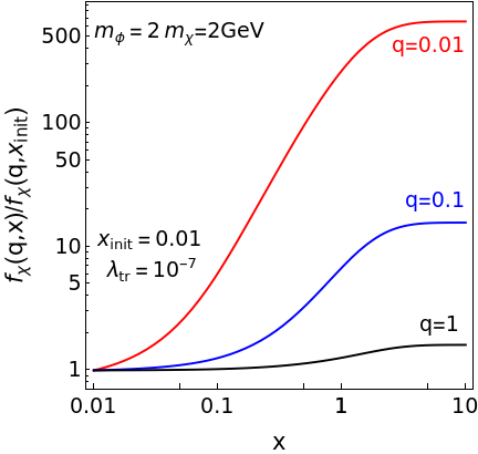
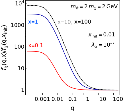
Figure 1: In the left panel, we display the evolution of the specific momentum modes in the scaled dark matter distribution function i.e. $f_{\chi}(q,x)/f_{\chi}(q,x_{\rm init})$ with the expansion of the universe. In the right panel, we show the scaled distribution function as a function of momentum at different epochs of the expansion history of the universe.

In our manuscript, we consider the scenarios where $m_{\phi}=2m_{\chi}$. In this case, during the epochs when exponential production of dark matter is active $s-4m_{\chi}^{2}\approx s$. The dependency of growth function on the comoving momentum in this case comes largely from $E_{q}$ in eqn. (16). To visualise how different modes grow with the expansion of the universe, in left panel of figure 1, we plot the scaled dark matter distribution function i.e. $f_{\chi}(q,x)/f_{\chi}(q,x_{\rm init})$ or $\exp[\int dxP^{\prime}(q,x)]$ (see eqn. 6) for some specific choices of q. It can be seen that lower momentum modes grow faster with the expansion of the universe. After certain epoch, the scattering becomes Boltzmann suppressed and the growth of all modes freezes. This can also be viewed in a different plotting frame in the right panel of figure 1. It can be seen that the growth of the dark matter momentum modes becomes identical for higher $x$’s (see lines from x=10 and x=100 are coinciding in figure 1) which specifies that the production of dark matter through $\chi+\phi\to\chi+\chi$ scattering has stopped.

If the initial mechanism populates all the momentum modes, then the lower momentum modes get more populated. In such cases it is hard to parameterise $A(x)$ in terms of some known function. However for cases where only extremely high momentum modes of dark matter are populated, the growth function $P^{\prime}(q,x)$ scales as $xK_{1}(x)$ where $K_{1}(x)$ is the first-order modified Bessel’s function. In this case, the growth of the dark matter momentum modes in the early universe for $x<1$ is simple exponential with the identification of $A(x)\propto x$. It can be seen from the left panel of figure 1 that the growth of higher momentum mode i.e. $q=1$ is indeed exponential.

4 Initial conditions

In order to compute the final relic abundance of the dark matter, it can be seen from eqn. (6) that we also need to determine the distribution function of dark matter at epoch $x_{\rm init}$. There could be several processes which could have populated the initial abundance of the dark matter. For the formalism of the previous section to be valid, those processes must be active in the UV and contribute negligibly during the epoch of exponential growth. We discuss two examples with freeze-in and out-of-equilibrium decay of a non-relativistic particle in the following sections 4.1, 4.2. Note that although the mechanisms generating the initial dark matter abundance contribute negligibly to the dark matter number density, however it’s knowledge is important from the point of view of population of initial momentum modes in the dark matter phase distribution function. In particular, different mechanisms can populate different momentum modes resulting in different final phase space distribution and hence the abundance.

4.1 Freeze-in

In this section, we discuss the initial dark matter production through Freeze-in Hall:2009bx . The toy model described in previous section can also naturally give rise to interactions leading to dark matter production through freeze-in:

$$\mathcal{L}_{\rm int}\subset\frac{\lambda_{\rm fi}}{2}\chi^{*}\chi\phi^{2}\;.$$ (17)

Even if the above interaction is absent at the tree-level, it can naturally be generated at one-loop order and contribute to dark matter production. For the exponential growth mechanism to be the dominant production of dark matter, the scalar coupling $\lambda_{\rm fi}$ must be much smaller than the optimal coupling required to generate the correct relic abundance of $\Omega h^{2}=0.12$ solely through the freeze-in process for the given dark matter and mediator mass. However it must be non-zero in order to generate the negligibly small initial dark matter number density. In Fig. 2, we give timeline of dark matter production in this case.

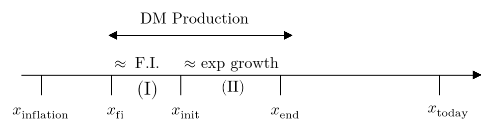
Figure 2: The figure shows the timeline of dark matter production with freeze-in generating the initial dark matter abundance to onset its exponential production. The epochs $x_{\rm fi}$ and $x_{\rm init}$ represent the onset of freeze-in and exponential growth of dark matter respectively. At $x_{\rm end}$, the dark matter number density freezes, and its production stops. In region (I), freeze-in dominates, and in region (II) exponential growth dominates.

We define epochs where different production mechanisms are active. After the period of inflation, the universe is radiation dominated with the thermal bath defined by standard model particles and $\phi$. We assume that inflaton decay does not produce dark matter particles. Due to interactions present between the bath particle ($\phi$) and dark matter ($\chi$) as described in eqn. (17), at some epoch defined by $x_{\rm fi}$, dark matter production through freeze-in begins. The bath particle scatters to produce dark matter particles i.e. $\phi(k)\phi(k^{\prime})\to\chi(p)\chi^{*}(p^{\prime})$. This generates the initial dark matter density. The exponential growth mechanism begins at the epoch $x_{\rm init}$. From epochs $\left(x_{\rm init},x_{\rm end}\right)$, the dark matter production is dominated by exponential growth which halts at $x_{\rm end}$ with the process becoming Boltzmann suppressed and resulting in freezing of dark matter comoving number density. We can compute the final relic abundance here using three methods. In first method, we use the general approach discussed in section 2 to obtain first the distribution function, and then the relic abundance. In order to compare our results with the literature, in the second method, we use the approximation of dark matter distribution function tracing the equilibrium pattern and determine the final abundance for our toy model. The solutions in both cases are obtained analytically. In the third method, we compute the dark matter distribution function by again solving the Boltzmann equation at operator level. However in this case, we take into account the contributions of both freeze-in and exponential growth till $x_{\rm end}$ approach and determine the solutions numerically. We then compare our results obtained using different methods.

4.1.1 Method-1

Since Freeze-in and exponential growth are active in different epochs, we can split the Boltzmann equation into two regions (I) and (II). The solution of B.E. in region (I) gives the initial distribution function which is used as initial condition to the Boltzmann equation in region (II). We use the technique described in section 2 to obtain the results. The collision operator in region (I) dominated by freeze-in is given as:

$$\mathcal{C}^{\rm(I)}[f_{\chi}(q,x)] \approx \frac{1}{2E_{q}\;S}\int\frac{d^{3}p^{\prime}}{(2\pi)^{3}2E_{p^{\prime}}}\frac{d^{3}k}{(2\pi)^{3}2E_{k}}\frac{d^{3}k^{\prime}}{(2\pi)^{3}2E_{k^{\prime}}}(2\pi)^{4}\delta^{4}\big{(}[s(x)]^{1/3}q+p^{\prime}-k-k^{\prime}\big{)}$$ (18)

$$\quad\quad\quad\times\;f^{\rm eq}_{\chi}(q,x)f^{\rm eq}_{\chi}(p^{\prime},x)\;|M|^{2}_{\phi\phi\to\chi\chi}\quad\left[\text{for}\quad x_{\rm fi}<x<x_{\rm init}\right]$$

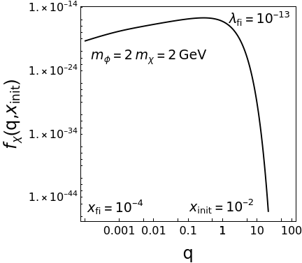
Figure 3: In this figure, we plot $f_{\chi}(q,x_{\rm init})$ obtained for the case of freeze-in.

Here the matrix amplitude squared term $|M|^{2}_{\phi\phi\to\chi\chi}$ is $|\lambda_{\rm fi}|^{2}$ and the symmetry factor is two. Note that for writing the freeze-in term, we have used principle of detailed balance and have expressed the distribution function of the bath particle in terms of the dark matter particles to perform momentum integrals $k$ and $k^{\prime}$. Solving Boltzmann equation in Region (I) is simple as in the case of freeze-in too and we can neglect the backward scattering processes. The distribution function of dark matter obtained from freeze-in at epoch $x_{\rm init}$ is given as

$$f_{\chi}(q,{x_{\rm init}}) = {{\int}}^{x_{\rm init}}_{x_{\rm fi}}dx\frac{|\lambda_{\rm fi}|^{2}h_{\rm eff}(x)f^{\rm eq}_{\chi}(q,x)}{32\pi E_{q}\;x\;H(x)}\int\frac{d^{3}p^{\prime}}{(2\pi)^{3}2E_{p^{\prime}}}\frac{\sqrt{s-4m_{\chi}^{2}}}{\sqrt{s}}f^{\rm eq}_{\chi}(p^{\prime},x)\;.$$ (19)

In figure 3, we plot the initial distribution function of dark matter obtained after freeze-in for some specific choices of couplings and mass.

Integrating the distribution function over full phase space gives the initial comoving number density ($Y_{\chi}(x=x_{\rm init})$) which can be used to estimate the freeze-in coupling i.e. $\lambda_{\rm fi}$. This initial distribution function, along with the growth function in eqn. (16) can be used to determine the dark matter distribution at the epoch $x_{\rm end}$ (where the exponential growth freezes) as:

$$f_{\chi}(q,x_{\rm end})=f_{\chi}(q,x_{\rm init})\exp{\left(\int_{x_{\rm init}}^{x_{\rm end}}dx\;\frac{P^{\prime}(q,x)}{x\;}\right)}$$ (20)

The final abundance of dark matter which is a function of the couplings $\lambda_{\rm tr}$, $\lambda_{\rm fi}$ and the masses $m_{\phi}$ and $m_{\chi}$, can be computed by computing the zeroth moment of the distribution function in eqn. (20).

4.1.2 Method-2

In order to compare our result with the existing analysis in the literature Bringmann:2021tjr , we determine the abundance for the case when the distribution function is approximated to trace the equilibrium pattern. In this case, the final relic abundance is given in eqn. (12) and is independent of the process generating initial density. However, in order to compare our predictions with Method-1 which is sensitive to the details of the process generating initial conditions, we assume that the initial abundance here is also produced by freeze-in. We determine the coupling $\lambda_{\rm fi}$ for a fixed value of $Y_{\chi}(x=x_{\rm init})$ as

$$Y_{\chi}(x_{\rm init})=\int_{x_{\rm fi}}^{x_{\rm init}}dx\;\frac{h_{\rm eff}(x)\;[n_{\chi}^{{\rm eq}}(x)]^{2}\;\langle\sigma v\rangle_{\rm fi}}{2\;s(x)\;H(x)\;x}\;.$$ (21)

The thermal average cross-section $\langle\sigma v\rangle_{\rm fi}$ for freeze-in is given in eqn. (29). Using this, the final comoving number density of dark matter particles can be given as:

$$Y_{\chi}(x)=\int_{x_{0}}^{x_{\rm init}}dx\;\frac{h_{\rm eff}(x)\;[n_{\chi}^{{\rm eq}}(x)]^{2}\;\langle\sigma v\rangle_{\rm fi}}{2\;s(x)\;H(x)\;x}\;\times\exp{\left(\int_{x_{\rm init}}^{x}dx\;\frac{h_{\rm eff}(x)\;n_{\phi}^{\rm eq}(x)\langle\sigma v\rangle_{\rm tr}}{2\;H(x)x}\right)}$$ (22)

Here the thermal average cross-section $\langle\sigma v\rangle_{\rm tr}$ required for exponential growth is given eqn. (28).

4.1.3 Method-3

The approximation used in Method-1 is fully justified if the freeze-in was dominated in the ultra-violet. However, the freeze-in generated by interaction in eqn. (17) also contributes at infra-red. It may not have significant contributions in setting up the relic when exponential growth is the dominant mechanism, but it can alter the distribution function. To compute this effect, we solve the Boltzmann equation numerically by considering the full collision operator i.e.

$$\mathcal{C}[f_{\chi}(q,x)]=\mathcal{C}^{\rm(I)}[f_{\chi}(q,x)]+\mathcal{C}^{\rm(II)}[f_{\chi}(q,x)]\;.$$ (23)

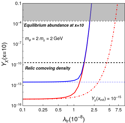
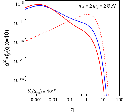
Figure 4: The left panel of the figure compares the relic abundance for three methods described in text. The initial dark matter abundance is considered to be $Y_{\chi}(x_{\rm init})=10^{-15}$. In the right panel, we compare probabilities of finding dark matter with comoving momentum in the range $(q,q+dq)$. The red solid line represents the results obtained from method-1, red dot-dashed line represents the results from method-2, and blue-solid line represents the results obtained from method-3. The gray shaded portions corresponds to the regions where the backward scatterings ($\chi\chi\to\chi\phi$) can no longer be neglected.

4.1.4 Results

We present our results obtained using Method-1,2 and 3 in figure 4. In the left panel, we display the dark matter comoving density as a function of the coupling $\lambda_{\rm tr}$. In the right panel, we display the probability of finding dark matter in the comoving momentum range (q,q+dq) as a function of comoving momentum ($q$). The red solid line represents the results obtained from method-1, red dot-dashed line represents the results from method-2, and blue-solid line represents the results obtained from method-3. Note that the predictions for method-2 matches with the results obtained in the reference Bringmann:2021tjr and serve as a validation for our analysis.

We have displayed the results for the case when the initial comoving density of dark matter is $Y_{\chi}(x=x_{\rm init})=10^{-15}$ which corresponds to $\lambda_{\rm fi}=1.064\times 10^{-12}$. We choose $x_{\rm fi}$, $x_{\rm init}$ and $x_{\rm end}$ as $10^{-4}$, $10^{-2}$ and 10 respectively for our analysis. The near exponential growth results in regions where $s-4m_{\chi}^{2}\approx s$, we implement this approximation in our calculation. For illustration, we have fixed the masses of bath particle ($\phi$) and dark matter ($\chi$) to be 2 GeV and 1 GeV respectively. The condition requiring $m_{\phi}\leq 3m_{\chi}$ to avoid the dark matter production in decays of $\phi$ sets a lower limit on the mass of the dark matter particle. The constraints from Big Bang Nucleosynthesis demand $m_{\phi}\geq\mathcal{O}$(few) MeV BBN . Therefore, dark matter mass in this case must also be larger than MeV. Note that the distribution function for $\phi$ is chosen to be Maxwell-Boltzmann. As we are focusing on scenarios with $m_{\phi}>m_{\chi}$, therefore the exponential growth is active close to regions where $\phi$ turns non-relativistic. Hence the choice of treating the phase space distribution of $\phi$ classically is a good approximation.

We need to draw important differences between method 1 and 2, and method 1 and 3. We begin with the former case. Note that for smaller range of the couplings $\lambda_{tr}$, the predictions of method-1 and method-2 matches. This is because for these couplings the contribution to dark matter abundance from exponential growth has not picked up yet. For high enough couplings, we see striking departures in the predictions of the two cases. The coupling required to explain the dark matter relic abundance using method-1 is smaller than method-2. In the right panel of figure 4, we compare probability of finding dark matter with comoving momentum in the range ($q,q+dq$). In dot-dashed lines, we assume that the distribution function follows the equilibrium behavior as described in eqn. (1), while in red-solid lines, the distribution function obtained by directly solving the BE using method-1 is displayed. Here also striking differences between the two cases can be noted. The probabilities are plotted for the end epoch at x=10. After this epoch, the comoving distribution function freezes because dark matter production stops. While for the equilibrium distribution, it is expected that the probability of finding dark matter peaks around $q\approx 1$. For the distribution function obtained by directly solving Boltzmann equation, the probability peaks for smaller values of the comoving momentum. Hence dark matter distribution obtained by solving BE is colder than the equilibrium distribution.

We now compare method-1 and method-3. It can be seen from left panel of fig 4, for smaller values of $\lambda_{\rm tr}$, when exponential growth is not the dominant mechanism, the final abundance between the two methods are different. This is because in method-3 we calculate the final abundance by considering the effect of freeze-in till $x_{\rm end}$, and in method-1, we compute the effect of freeze-in only until $x_{\rm init}$. However, for larger $\lambda_{\rm tr}$, when the production of dark matter dominates due to the exponential growth mechanism, the predictions of two methods converge, as in these cases, neglecting freeze-in in region-II serves to be a good approximation. However, while considering probabilities of finding dark matter with the comoving momentum ($q,q+dq$), there is a slight change due to the inclusion of the freeze-in in total collision process. The probabilities still peak at lower values of comoving momentum, however there is a slight inclination towards $q\sim 1$ in method-3 due to presence of freeze-in scatterings.

To conclude this section, we find that our results by computing the distribution function directly from solving the Boltzmann equation either method-1 or method-3 differ significantly from the method-2 where equilibrium form is assumed.

4.2 Out-of equilibrium decay of a non-relativistic particle

To illustrate the dependence on the initial conditions, as a second example, we consider the initial production of dark matter, at some epoch $x_{\rm init}$, from the non-thermal decay of a non-relativistic scalar particle ($\Phi$). We consider its mass to be much greater than the mass of the dark matter particle. The initial distribution function of dark matter can be determined by solving the Boltzmann equation which in this case is also a simplified equation because of negligible inverse process $\chi^{*}\chi\to\Phi$. The solution of the Boltzmann equation for dark matter depends on the distribution function of $\Phi$ i.e. $f_{\Phi}$ or in other words on the details of $\Phi$ production in the early universe . However, since we are considering the scenario where $m_{\chi}\ll m_{\Phi}$, the momentum of the dark matter produced through decays of $\Phi$ peaks roughly around $m_{\Phi}/2$. Owing to this simplification, it is possible to simplify the analysis and heuristically parameterize the distribution function of the dark matter independent of the details of the production of $\Phi$ Ghosh:2022hen as

$$f_{\chi}(q,x)=A\;\delta{\left(|q|-q_{\rm init}\right)}\;\Theta\left(x-x_{\rm init}\right)\;.$$ (24)

Here $q_{\rm init}={m_{\Phi}}/{\left(2\;[s(x_{\rm init})]^{1/3}\right)}$ and $A$ is a parameter which depends on the specific details of $\Phi$ production and its couplings with the dark matter. It can be inferred in a model independent manner by specifying the initial comoving dark matter number density $Y_{\chi}(x=x_{\rm init})$ as

$$A=\frac{2\pi^{2}\;Y_{\chi}(x=x_{\rm init})}{q_{\rm init}^{2}}\;.$$ (25)

As before, the initial dark matter density $Y_{\chi}(x=x_{\rm init})$ obtained from decay of $\Phi$ is assumed to be much smaller than its abundance today $Y_{\chi}(x=x_{\rm today})$, with exponential growth mechanism as the dominant source of dark matter abundance. Note that the decay of $\Phi$ is considered to be instantaneous in our analysis. With the initial distribution function in eqn. (24), we can estimated the final distribution function, using the toy model in section 3 as:

$$f_{\chi}(q,x)=\frac{2\pi^{2}\;Y_{\chi}(x=x_{\rm init})}{q_{\rm init}^{2}}\;\delta{\left(|q|-q_{\rm init}\right)}\exp{\left(\int_{x_{\rm init}}^{x}dx\;{P^{\prime}(q,x)}\right)}\;\Theta\left(x-x_{\rm init}\right)\;.$$ (26)

The growth function $P^{\prime}(q,x)$ for the toy model is given in eqn. (16). The dark matter relic abundance can be computed by evaluating zeroth moment of the distribution function as

$$Y_{\chi}(x) = \int\frac{d^{3}q}{(2\pi)^{3}}\;\bigg{[}A\;\delta{\left(|q|-q_{\rm init}\right)}\exp{\left(\int_{x_{\rm init}}^{x}dx\;{P^{\prime}(q,x)}\right)}$$ (27)

$$= Y_{\chi}(x=x_{\rm init})\;\bigg{[}\exp{\left(\int_{x_{\rm init}}^{x}dx\;{P^{\prime}(q_{\rm init},x)}\right)}\bigg{]}$$

Since the distribution function peaks at very high comoving momentum values, therefore from the discussion in section 3, we find that the growth of dark matter distribution function is exponential and $A(x)\propto x$. The relic abundance in this simplified treatment depends on the initial momentum transferred to the dark matter particles, and on the initial abundance. The relic distribution function in the comoving frame peaks at $q_{\rm init}$ which is strikingly different from the equilibrium distribution following a Maxwell-Boltzmann pattern. Note that although our treatment of this section is simplified but it highlights the essence that the obtained dark matter distribution function is remarkably different from the equilibrium distribution. This conclusion is robust and holds true in the case of negligible scatterings between the dark matter, and the bath particles. The presence of finite yet negligible scatterings between the dark matter and bath particles mediated by $\Phi$ will cause the dark matter distribution to spread around $q_{\rm init}$. The distribution function is still expected to be different from the equilibrium distribution if these scatterings are sub-dominant.

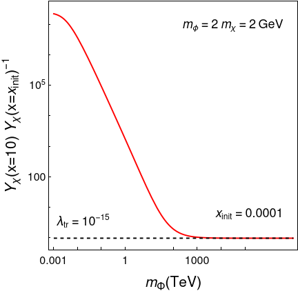
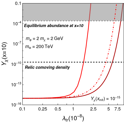
Figure 5: In the left panel, we plot the ratio of dark matter abundances at $x=10$ with its initial abundance generated by decay of $\Phi$ as a function of $m_{\Phi}$. The dashed line corresponds to the case where $Y_{\chi}(x=10)=Y_{\chi}(x=x_{\rm init})$. The right panel of the figure compares different mechanisms generating dark matter initial abundance. The first scenario is when a particle of mass $m_{\Phi}=200$ TeV decays non-thermally to produce initial density of the dark matter. The predictions are plotted in dark red solid line. The other two scenarios are the cases where the initial dark matter density is produced through freeze-in. In red solid line, we plot the predictions from method-1 and in red dot-dashed lines, predictions from method-2 are plotted.

We present results of this scenario in figure 5. In the left panel, we display the ratio of dark matter abundances at $x=10$ with its initial abundance generated by decay of $\Phi$ as a function of $m_{\Phi}$. We chose $\lambda_{\rm tr}=10^{-7}$. It can be seen that for very high values of mass of $\Phi$, the exponential growth does not contribute in dark matter production for the chosen coupling $\lambda_{\rm tr}$. This can be seen from the fact that $Y_{\chi}(x=10)\to Y_{\chi}(x=x_{\rm init})$. This happens because for larger values of $m_{\Phi}$, very high momentum modes of dark matter gets populated, and consequently the growth function $P^{\prime}(q,x)\to 1/q$ approaches zero. Note that the mass of $\Phi$ above which the exponential growth cease to contribute to dark matter production depends on the coupling $\lambda_{\rm tr}$. For higher values of $\lambda_{\rm tr}$, larger values of $m_{\Phi}$ up to which exponential growth is active are allowed.

In the right panel of figure 5, we display $Y_{\chi}$ as a function of $\lambda_{\rm tr}$ at epoch $x=10$ where the number density of dark matter has already frozen. Since we assume the adiabatic expansion of the universe, the comoving density of dark matter stays the same till the present epoch. We chose $m_{\Phi}=200$ TeV for the purpose of this plot. In the same plot to draw comparisons between different scenarios, we also show predictions from Method-1 and Method-2. It can be seen that for the chosen case, larger value of $\lambda_{\rm tr}$ coupling is required to establish the correct abundance. The regions shaded in dark gray indicate that we can no longer ignore the backward scatterings as the comoving densities become of the order of the equilibrium densities. However from the figure, we can see that the coupling required to reproduce the relic abundance is well below the equilibrium density. Hence our choice of ignoring the backward scattering contributions in the collision terms, and Pauli-Blocking/Bose enhancement factors is justified.

In this scenario, dark matter is produced relativistically. Hence it must be sufficiently red-shifted during the epochs of matter-radiation domination to avoid constraints from the structure formation. A naive bound from the structure formation can be derived by putting constraints on the dark matter comoving free streaming length at epoch of matter-radiation equality Kolb:1990vq . For our choices of masses, we satisfy this constraint.

5 Summary and concluding remarks

In this manuscript, we revisit the exponential growth production mechanism of dark matter. In the literature Bringmann:2021tjr ; Hryczuk:2021qtz ; Bringmann:2022aim , the results are obtained using the simplified assumption of dark matter phase space tracing the equilibrium distribution. Owing to the non-thermal nature of the problem, we solve the Boltzmann equation at the operator level to determine the final distribution function.

Note that the scattering $\chi+\phi\to\chi+\chi$ is an initial-condition dependent problem. Therefore, it is highly sensitive to the process populating the initial dark matter momentum modes. We assume that dominant production of dark matter proceeds through the $\chi+\phi\to\chi+\chi$ scattering and the initial process contributes negligibly to the dark matter abundance. However, even if the initial mechanism generates a negligible amount of dark matter number density, its knowledge is important from the point of view of populating the dark matter momentum modes and correspondingly their evolution with the expansion of the universe.

Since we solve for the un-integrated Boltzmann equation, it becomes useful to describe the growth in terms of the evolution of the momentum modes of the dark matter distribution function with the expansion of the universe rather than the number density. The distribution function freezes when the $\chi+\phi\to\chi+\chi$ scattering becomes Boltzmann suppressed. The growth of a given momentum mode can be generically described by an exponential factor viz. $\exp[A(x)]$ with $A(x)$ depending on the details of the model. On the other hand, the growth of the dark matter number density a complicated function of $x$ depending on $A(x)$. In this manuscript, we continue to label the dark matter distribution function as exponential.

We consider a simple toy model containing a scalar dark matter charged under $Z_{3}$ symmetry. Its interactions with the bath particle $\phi$ onsets the exponential growth of the dark matter which stops with the rate of reaction becoming Boltzmann suppressed. To generate the initial abundance of dark matter, we consider two examples — Freeze-in and out-of-equilibrium decay of a non-relativistic particle. With freeze-in, the dark matter is found to have a colder distribution in comparison to the equilibrium distribution, and the non-thermal decay of the heavy particle makes the dark matter distribution to peak at either higher or lower values of comoving momenta in comparison to $q=1$ depending on the choices of the masses.

Note that in our computation we have made a few assumptions. The first assumption is regarding neglecting the Pauli-Blocking/Bose enhancement factors. This approximation seems fine in the limit of the dark matter density being extremely smaller than the equilibrium density. We have also approximated the distribution function of the bath particle $\phi$ to be the Maxwell-Boltzmann distribution function. As we worked out examples where $m_{\phi}>m_{\chi}$, the exponential growth is relevant just before $\phi$ turns non-relativistic, hence this approximation holds good to a good accuracy. For the opposite cases, where dark matter is heavier than the mass of the bath particle, it would be essential to include quantum statistics in the distribution function. In our computation, we consider that effects of elastic scattering present between the bath particles and dark matter is negligible. Inclusions of these scatterings can alter the dark matter distribution function, and it would be interesting to work out the limit when they can be important. We leave this part for the future work.

There are several directions in which the present work can be extended. We can consider the effects of other non-thermal production mechanisms which generate the initial dark matter abundance and find the correlation with the already considered examples. In our work, we considered $\phi$ to be coupled to a standard model bath. The results will change if $\phi$ was coupled to a hidden sector bath Hryczuk:2021qtz ; Bringmann:2022aim , was a non-thermal particle Belanger:2020npe . It would be interesting to work out these cases. The exponential growth mechanism is non-thermal in nature with low detectability prospects at experiments, however the distribution function of dark matter in these cases can potentially receive constraints from structure formation Boehm:2004th ; Ballesteros:2020adh ; DEramo:2020gpr ; Decant:2021mhj ; Yin:2023jjj. Hence it becomes essential to determine the distribution function for such processes using first principles, and determine the constraints using structure formation.

Appendix A The thermal averaged cross-sections

In this appendix, we list the thermal averaged cross-sections for the exponential growth mechanism and freeze-in production of dark matter. While computing these averages, it is assumed that dark matter traces the equilibrium distribution of the standard model. Note that for exponential growth, the thermal averaged formula takes into account the mass differences of the colliding particles $\phi$ and $\chi$, that is why the obtained formula is slightly different from the conventional case Gondolo:1990dk .

$$\langle\sigma v\rangle_{\rm tr} = \frac{2\pi^{2}T}{n_{\chi}^{\rm eq}(T)n_{\phi}^{\rm eq}(T)}\int_{\left(m_{\chi}+m_{\phi}\right)^{2}}^{\infty}\frac{\sigma_{\rm tr}}{\sqrt{s}}\left(s-(m_{\phi}-m_{\chi})^{2}\right)\left(s-(m_{\chi}+m_{\phi})^{2}\right)K_{1}{\left(\frac{\sqrt{s}}{T}\right)}\;\text{where}\;,$$

$$\sigma_{\rm tr} = \frac{|\lambda|_{\rm tr}^{2}}{16\pi\sqrt{s}}\frac{\sqrt{s-4m_{\chi}^{2}}}{\left(s-\left(m_{\phi}-m_{\chi}\right)^{2}\right)^{1/2}\left(s-\left(m_{\phi}+m_{\chi}\right)^{2}\right)^{1/2}}\;.$$ (28)

For the freeze-in case ($\phi\phi\to\chi\chi^{*}$), the thermally averaged cross-section given as:

$$\langle\sigma v\rangle_{\rm fi} = \frac{2\pi^{2}T}{n_{\chi}^{2,\rm eq}(T)}\int_{4m_{\chi}^{2}}^{\infty}\sigma_{\rm fi}{\sqrt{s}}\left(s-4m_{\chi}^{2}\right)K_{1}{\left(\frac{\sqrt{s}}{T}\right)}\;\bigg{[}\text{where}\;\sigma_{\rm fi}=\frac{|\lambda|_{\rm fi}^{2}\sqrt{s-4m_{\phi}^{2}}}{16\pi s\sqrt{s-4m_{\chi}^{2}}}\bigg{]}\;.$$ (29)

References

- (1) E.W. Kolb and M.S. Turner, The Early Universe, vol. 69 (1990), 10.1201/9780429492860.
- (2) J.L. Feng, Dark Matter Candidates from Particle Physics and Methods of Detection, Ann. Rev. Astron. Astrophys. 48 (2010) 495 [1003.0904].
- (3) XENON collaboration, Search for New Physics in Electronic Recoil Data from XENONnT, Phys. Rev. Lett. 129 (2022) 161805 [2207.11330].
- (4) ATLAS collaboration, Status of searches for dark matter at the LHC, Tech. Rep. ATL-PHYS-PROC-2022-003, CERN, Geneva (2022).
- (5) ATLAS, CMS collaboration, Dark Matter searches at CMS and ATLAS, in 56th Rencontres de Moriond on Electroweak Interactions and Unified Theories, 1, 2023 [2301.10141].
- (6) H. Baer, K.-Y. Choi, J.E. Kim and L. Roszkowski, Dark matter production in the early Universe: beyond the thermal WIMP paradigm, Phys. Rept. 555 (2015) 1 [1407.0017].
- (7) L. Parker, Quantized fields and particle creation in expanding universes. 1., Phys. Rev. 183 (1969) 1057.
- (8) L. Parker, Quantized fields and particle creation in expanding universes. 2., Phys. Rev. D 3 (1971) 346.
- (9) L.H. Ford, Cosmological particle production: a review, Rept. Prog. Phys. 84 (2021) [2112.02444].
- (10) L.J. Hall, K. Jedamzik, J. March-Russell and S.M. West, Freeze-In Production of FIMP Dark Matter, JHEP 03 (2010) 080 [0911.1120].
- (11) Y. Hochberg, E. Kuflik, T. Volansky and J.G. Wacker, Mechanism for Thermal Relic Dark Matter of Strongly Interacting Massive Particles, Phys. Rev. Lett. 113 (2014) 171301 [1402.5143].
- (12) M. Pospelov, A. Ritz and M.B. Voloshin, Bosonic super-WIMPs as keV-scale dark matter, Phys. Rev. D 78 (2008) 115012 [0807.3279].
- (13) J.L. Feng, H. Tu and H.-B. Yu, Thermal Relics in Hidden Sectors, JCAP 10 (2008) 043 [0808.2318].
- (14) T. Bringmann, P.F. Depta, M. Hufnagel, J.T. Ruderman and K. Schmidt-Hoberg, Dark Matter from Exponential Growth, Phys. Rev. Lett. 127 (2021) 191802 [2103.16572].
- (15) A. Hryczuk and M. Laletin, Dark matter freeze-in from semi-production, JHEP 06 (2021) 026 [2104.05684].
- (16) F. D’Eramo and J. Thaler, Semi-annihilation of Dark Matter, JHEP 06 (2010) 109 [1003.5912].
- (17) T. Bringmann, P.F. Depta, M. Hufnagel, J. Kersten, J.T. Ruderman and K. Schmidt-Hoberg, Minimal sterile neutrino dark matter, Phys. Rev. D 107 (2023) L071702 [2206.10630].
- (18) P. Gondolo and G. Gelmini, Cosmic abundances of stable particles: Improved analysis, Nucl. Phys. B 360 (1991) 145.
- (19) T. Binder, T. Bringmann, M. Gustafsson and A. Hryczuk, Early kinetic decoupling of dark matter: when the standard way of calculating the thermal relic density fails, Phys. Rev. D 96 (2017) 115010 [1706.07433].
- (20) R.T. D’Agnolo, D. Pappadopulo and J.T. Ruderman, Fourth Exception in the Calculation of Relic Abundances, Phys. Rev. Lett. 119 (2017) 061102 [1705.08450].
- (21) ATLAS collaboration, Combined measurements of Higgs boson production and decay using up to fb-1 of proton-proton collision data at 13 TeV collected with the ATLAS experiment, Phys. Rev. D 101 (2020) 012002 [1909.02845].
- (22) ATLAS collaboration, A detailed map of Higgs boson interactions by the ATLAS experiment ten years after the discovery, Nature 607 (2022) 52 [2207.00092].
- (23) G.B. Arfken, H.J. Weber and F.E. Harris, Chapter 14 - bessel functions, in Mathematical Methods for Physicists (Seventh Edition), G.B. Arfken, H.J. Weber and F.E. Harris, eds., (Boston), pp. 643–713, Academic Press (2013), DOI.
- (24) Big Bang Nucleosynthesis, https://pdg.lbl.gov/2020/reviews/rpp2020-rev-bbang-nucleosynthesis.pdf.
- (25) L. Kofman, A.D. Linde and A.A. Starobinsky, Reheating after inflation, Phys. Rev. Lett. 73 (1994) 3195 [hep-th/9405187].
- (26) G. Ballesteros, M.A.G. Garcia and M. Pierre, How warm are non-thermal relics? Lyman- bounds on out-of-equilibrium dark matter, JCAP 03 (2021) 101 [2011.13458].
- (27) A. Ghosh and S. Mukhopadhyay, Momentum distribution of dark matter produced in inflaton decay: Effect of inflaton mediated scatterings, Phys. Rev. D 106 (2022) 043519 [2205.03440].
- (28) G. Bélanger, C. Delaunay, A. Pukhov and B. Zaldivar, Dark matter abundance from the sequential freeze-in mechanism, Phys. Rev. D 102 (2020) 035017 [2005.06294].
- (29) C. Boehm and R. Schaeffer, Constraints on dark matter interactions from structure formation: Damping lengths, Astron. Astrophys. 438 (2005) 419 [astro-ph/0410591].
- (30) F. D’Eramo and A. Lenoci, Lower mass bounds on FIMP dark matter produced via freeze-in, JCAP 10 (2021) 045 [2012.01446].
- (31) Q. Decant, J. Heisig, D.C. Hooper and L. Lopez-Honorez, Lyman- constraints on freeze-in and superWIMPs, JCAP 03 (2022) 041 [2111.09321].