A scalable clustering algorithm to approximate graph cuts

Abstract

Due to its computational complexity, graph cuts for cluster detection and identification are used mostly in the form of convex relaxations. We propose to utilize the original graph cuts such as Ratio, Normalized or Cheeger Cut in order to detect clusters in weighted undirected graphs by restricting the graph cut minimization to the subset of $st$-MinCut partitions. Incorporating a vertex selection technique and restricting optimization to tightly connected clusters, we therefore combine the efficient computability of $st$-MinCuts and the intrinsic properties of Gomory-Hu trees with the cut quality of the original graph cuts, leading to linear runtime in the number of vertices and quadratic in the number of edges. Already in simple scenarios, the resulting algorithm Xist is able to approximate graph cut values better empirically than spectral clustering or comparable algorithms, even for large network datasets. We showcase its applicability by segmenting images from cell biology and provide empirical studies of runtime and classification rate.

1 Introduction

The detection and identification of clusters in datasets is a fundamental task of data analysis, with applications including image segmentation [38, 43, 47], machine learning [6, 41, 26], and parallel computing [49, 34, 5]. The construction and partitioning of a graph is key to many popular methods of cluster detection. Prominent graph cuts such as Ratio Cut [18], Normalized Cut [39] or Cheeger Cut [4] are designed to partition a graph in a “balanced” way while providing an intuitive geometric interpretation. Ratio Cut, for instance, attempts to balance cluster sizes, and Normalized Cut and Cheeger Cut aim for equal volumes of the resulting partitions. However, as the computation of the above mentioned cuts is an NP-hard problem (see e.g. [27, 3, 39, 40]), attention has shifted primarily to their various convex relaxations and regularizations. Most prominent are spectral clustering techniques, which can be viewed as a convex relaxation of the optimization problem underlying Normalized and Cheeger Cut [44]. They offer a quick and simple way to partition a graph, with a worst-case runtime cubic in the number of vertices [44], and their practical success has been demonstrated in numerous applications. Consequently, they have been the subject of extensive theoretical analysis [45, 25, 11] as well as the inspiration for a multitude of specialized algorithms [30, 29, 50]. However, it is well known that spectral clustering does not always yield a qualitatively sensible partition, the most famous example being the so-called “cockroach graph” and its variants [16]. More significantly, it has been shown that spectral clustering possesses fundamental flaws in detecting clusters of different scales [28].

To overcome these issues we propose a different approach which combines the versatility and quality of graph cuts with the most significant trait of spectral clustering, its quick and simple computability. While spectral clustering builds on Normalized Cut and Cheeger Cut alone, the suggested algorithm Xist is applicable to any balanced graph cut functional, thus making it adaptable and scalable. In contrast to spectral clustering, our algorithm approximates graph cuts not by means of relaxation of the graph cut functional, but instead by restricting minimization onto a particularly designed subset of partitions. This subset is constituted by $st$-MinCuts, where $s$ and $t$ runs through a certain subset of vertices. These partitions can be computed very fast through max flows [32] and the well-known duality of the max-flow and min-cut problems. Hence, our proposed algorithm Xist to a large extent preserves the combinatorial nature of the problem while retaining a worst computational complexity quadratic in the number of vertices and linear in the number of edges (Theorem 3.2).

The rest of the paper is organized as follows. Section 2 introduces the basic notation. The proposed 2-way cut algorithm is detailed in Section 3, together with its theoretical properties. In Section 4, we introduce a multiway cut extension and study the performance of the proposed algorithm on simulated and real world datasets. Section 5 provides a discussion of further extensions and concludes the paper. All proofs are given in the Appendix.

2 Definitions and notation

We consider simple, undirected, and weighted graphs, denoted as $G=(V,E,{\boldsymbol{W}})$, with $V$ the vertex set, $E$ the set of edges and ${\boldsymbol{W}}=(w_{ij})_{i,j\in V}$ the weight matrix. Each entry $w_{ij}$ equals the weight of edge $\{i,j\}$ if $\{i,j\}\in E$ and zero otherwise. Thus, ${\boldsymbol{W}}$ is symmetric and has a zero diagonal.

Definition 1 (Graph cut).

For a simple, undirected, weighted graph $G=(V,E,{\boldsymbol{W}})$, we define the (balanced) graph cut $\operatorname{\mathrm{XC}}$ of $G$ as:

$$\operatorname{\mathrm{XC}}(G) \coloneqq\min_{S\subset V}\operatorname{\mathrm{XC}}_{S}(G)$$

$$\text{where}\quad\operatorname{\mathrm{XC}}_{S}(G) \coloneqq\sum_{{i\in S,j\in{S}^{\mathsf{c}}}}\frac{w_{ij}}{\operatorname{Bal}_{G}(S,{S}^{\mathsf{c}})}$$

for $S\subset V$. Here, ${S}^{\mathsf{c}}\coloneqq V\setminus S$ is the complement of $S$, and $\operatorname{\mathrm{XC}}$ and $\operatorname{Bal}_{G}(S,{S}^{\mathsf{c}})$ serve as placeholders for the graph cut (see Table 1) and its corresponding balancing term, respectively.

Table 1 lists the balancing terms for Minimum Cut (MinCut), Ratio Cut, Normalized Cut (NCut) and Cheeger Cut. In general, these balancing terms can depend on the underlying graph structure, the partition $S$ as well as the weight matrix ${\boldsymbol{W}}$. For any partition $S\subset V$, define its size as $|S|\coloneqq\#\{i\in S\}$ and its volume as $\operatorname{vol}(S)\coloneqq\sum_{i\in S}\deg(i)$, where $\deg(i)\coloneqq\sum_{j\in V}w_{ij}$ is the degree of vertex $i$. Assume $n\coloneqq|V|<\infty$ and $m\coloneqq|E|<\infty$.

Table 1: Definitions of common (balanced) graph cuts.

Cut name	$\operatorname{\mathrm{XC}}$	$\operatorname{Bal}_{G}(S,{S}^{\mathsf{c}})$	Reference
Minimum Cut	$\operatorname{\mathrm{MC}}$	$1$	E.g. [8]
Ratio Cut	$\operatorname{\mathrm{RC}}$	$|S|\,|{S}^{\mathsf{c}}|$	[18]
Normalized Cut	$\operatorname{\mathrm{NC}}$	$\operatorname{vol}(S)\operatorname{vol}({S}^{\mathsf{c}})$	[39]
Cheeger Cut	$\operatorname{\mathrm{CC}}$	$\min\{\operatorname{vol}(S),\,\operatorname{vol}({S}^{\mathsf{c}})\}$	[4]

The disadvantage of (balanced) graph cuts is their computational complexity that is rooted in their combinatorial nature. It has been shown that the problem of computing NCut is NP-complete, see [39, Appendix A, Proposition 1], and the idea behind the proof can be adapted for the other balanced cuts in Table 1, namely Ratio Cut and Cheeger Cut (see [40] for an alternative proof for the latter). Several other balanced graph cuts are also known to be NP-complete to compute, for instance, the graph cut with the balancing term $\operatorname{Bal}_{G}(S,{S}^{\mathsf{c}})=\min\{|S|,|{S}^{\mathsf{c}}|\}$, see [27]. It should be noted that, due to its lack of a balancing term, MinCut is computable in polynomial time (see [13] for an algorithm in $\mathcal{O}(m\log^{2}n)$ time). For applications, however, MinCut is of limited relevance since it tends to separate a single vertex from the remainder of the graph [44]. Thus, all practically relevant graph cuts become non-computable even for problems of moderate sizes. This also remains the case for many relaxed versions [46] and approximations of graph cuts [3]. As mentioned in the Introduction, spectral clustering represents a notable exception as it can be regarded as a relaxation of Normalized and Cheeger Cut while still being computable in $\mathcal{O}(n^{3})$ time.

3 The algorithms

We first introduce the basic algorithm and then present a refined and vastly accelerated variant.

3.1 A basic algorithm for imitating graph cuts through $st$-min cuts

To retain the qualitative aspects of the (balanced) graph cuts themselves as much as possible we suggest to restrict the combinatorial optimization to a certain collection of partitions. Then, if such a collection of partitions is well-chosen, the original graph cut (i.e. the minimizer over all partitions) can be imitated on a qualitative level. For this purposes, we consider some collections of $st$-MinCut partitions, i.e. the cuts that separate the two nodes $s$ and $t$ in $V$ for $s,t\in V$. More precisely, an $st$-MinCut partition $S_{st}$ is defined as

$$S_{st}\; \in\;\operatorname*{arg\,min}_{S\in\mathcal{S}_{st}^{*}}\operatorname{\mathrm{MC}}_{S}(G),$$

$$\text{where}\quad\mathcal{S}_{st}^{*} \coloneqq\{S\subset V\;:\;s\in S,\ t\not\in S\}.$$

The partition $S_{st}$ might not be unique. In practice, the nonuniqueness represents a fringe case that is highly unlikely to occur on real-world data; this issue is discussed in more depth later. Also notice that, by definition, $s\in S_{st}$ and $t\in{S}^{\mathsf{c}}_{st}$ for any $s,t\in V$, $s\neq t$. This property will be important later. The fastest algorithms for computing an $st$-MinCut partition take $\mathcal{O}(nm)$ time for general graphs; for instance, one could use [32] if $m=\mathcal{O}(n^{1.06})$, and [33] otherwise, see also Section A.3.

Our idea is to restrict the graph cut minimization to the $st$-MinCut partitions. A first version of our algorithm is as follows:

input : weighted graph $G=(V,E,{\boldsymbol{W}})$

output : XC value $c_{\min}$ with associated partition $S_{\min}$

1

2set $c_{\min}\leftarrow\infty$ and $S_{\min}\leftarrow\emptyset$

3

4for $\{s,t\}\subset V$ with $s\neq t$ do

5       compute an $st$-MinCut partition $S_{st}$ on $G$

6       compute the graph cut value $\operatorname{\mathrm{XC}}_{{S}^{\mathsf{c}}_{st}}(G)$ of partition $S_{st}$

7       if $\operatorname{\mathrm{XC}}_{S_{st}}(G)<c_{\min}$ then

8             $c_{\min}\leftarrow\operatorname{\mathrm{XC}}_{S_{st}}(G)$

9             $S_{\min}\leftarrow S_{st}$

10            

11       end if

12      

13 end for

Basic Xvst algorithm 1 $\operatorname{\mathrm{XC}}(G)$ via $st$-MinCuts

As the computation of $st$-MinCut in line 1 of our basic Xvst algorithm is in $\mathcal{O}(nm)$ time, the complexity of this algorithm is $\mathcal{O}(n^{3}m)$ (Theorem 3.2). While this is not particularly fast, the design of the algorithm guarantees that the resulting partition is a cut that is reasonable in the sense that it separates two vertices $s$ and $t$ through the $st$-MinCut partition $S_{st}$ while also taking cluster size into account via the balancing term in the graph cut value $\operatorname{\mathrm{XC}}_{S_{st}}({G})$. This imitates the nature of the NP-complete problem of computing graph cuts from a qualitative perspective, whereas spectral clustering methods rely on convex relaxation of the corresponding functionals and therefore mainly approximate graph cuts on a quantitative level. More precisely, the partition $S_{\operatorname{min}}$ that the basic Xvst algorithm outputs is guaranteed to be an $st$-MinCut for some $s,t\in V$, whereas the partition returned by spectral clustering does not possess any inherent qualitative feature per se.

In the literature, the attention has mainly focused on the set $\mathcal{S}^{*}_{st}$ of $st$-MinCut partitions for a fixed pair of $s,t\in V$, $s\neq t$. For instance, the cardinality of $\mathcal{S}^{*}_{st}$ has been used as a structure characterization on the crossing minimization problem in graph planarizations [7]. Apart from this, [2] showed that the problem of finding the most balanced partition in $\mathcal{S}^{*}_{st}$ is NP-hard. In contrast, we consider only one $st$-MinCut partition $S_{st}$ for a given pair of $s,t\in V$, and employ instead the collection of such partitions for all pairs of $s,t\in V$, namely, $\{S_{st}\colon s,t\in V,s\neq t\}$. In this way, we preserve the intrinsic structure of the graph to a large extend while gaining efficient computation in polynomial time.

3.2 The proposed Xist algorithm

(a) All local maxima $v_{1}$, $v_{2}$, $v_{3}$, $v_{4}$.
Initially, $\tau=(1,1,1,1)$.

(b) $v_{2}v_{1}$-MinCut with $\operatorname{\mathrm{NC}}\approx 5.12$.
Updated $\tau=(1,2,2,2)$

(c) $v_{3}v_{2}$-MinCut with $\operatorname{\mathrm{NC}}\approx 0.70$.
Updated $\tau=(1,2,3,3)$

(d) $v_{4}v_{3}$-MinCut with $\operatorname{\mathrm{NC}}\approx 2.51$.
Still $\tau=(1,2,3,4)$

Figure 1: Illustration of the Xist algorithm for the NCut functional on a toy example, where the thickness of each edge $\{i,j\}\in E$ corresponds to its weight $w_{ij}$, and the size of each vertex $i\in V$ is proportional to its degree $\deg(i)$. (a) depicts the set of local maxima $\operatorname{V^{\mathrm{loc}}}=\{v_{1},v_{2},v_{3},v_{4}\}$. Xist computes first the $v_{2}v_{1}$-MinCut and updates $\tau$ (b), then the $v_{3}v_{2}$-MinCut with another update to $\tau$ (c). Finally, the $v_{4}v_{3}$-MinCut is computed, and $\tau$ is not updated further. Since the $v_{3}v_{2}$-MinCut in (c) gives the best NCut value among all three partitions, Xist outputs this partition and value.

We improve the basic Xvst algorithm by two techniques, see Figure 1 for an illustration.

First, we further restrict the minimization of the graph cut functional by only considering certain vertices $s$ and $t$ to compute the $st$-MinCuts over. In practice, $st$-MinCut partitions only become viable if one forces $s$ and $t$ to belong to tightly connected clusters to avoid a partition that cuts out only one vertex (this may happen as MinCut does not have a balancing term to counteract this). If $s$ and $t$ are connected to their respective neighbouring nodes through high-weighted edges, the $st$-MinCut cannot simply cut out one or the other and is therefore forced to find a different, more balanced way to separate both vertices. Formally, we call a vertex $u\in V$ a local maximum if $\deg(u)\geq\deg(v)$ for all $v\in V$ with $\{u,v\}\in E$. We denote the set of local maxima as

$$\operatorname{V^{\mathrm{loc}}}\coloneqq\bigl{\{}u\in V\mid \deg(u)\geq\deg(v)$$

$$\text{for all }v\in V\text{ with }\{u,v\}\in E\bigr{\}},$$

with its cardinality $|\operatorname{V^{\mathrm{loc}}}|=:N$. For a visualization of $\operatorname{V^{\mathrm{loc}}}$ see Figure 1 (a). By definition of $\operatorname{V^{\mathrm{loc}}}$, we can ensure the scenario described above by requiring both $s$ and $t$ to be local maxima.

Second, it is not necessary to iterate over all pairs $\{s,t\}\subset\operatorname{V^{\mathrm{loc}}}$ to obtain all $st$-MinCuts of vertices in $\operatorname{V^{\mathrm{loc}}}$. It is known that in a graph of $n$ vertices, there are at most $n-1$ distinct $st$-MinCuts, and that these can be computed through the construction of the so-called Gomory-Hu tree that was introduced by [15]. The Gomory-Hu tree is a tree built on $V$ where the edge weights are $st$-MinCut values, $s,t\in V$. [15] showed that this tree can be constructed through vertex contraction and only $n-1$ $st$-MinCut computations, and that it encapsulates all $st$-MinCut values. Consequently, there are only $n-1$ $st$-MinCuts, meaning that it is possible to improve the complexity of the basic Xvst algorithm by $\mathcal{O}(n)$. Additionally, their proofs can be adapted for the case that only those $st$-MinCuts are of interest where $s,t\in A$ for any subset $A\subseteq V$. We present this in Section A.2 of the Appendix.

Expanding upon this classical result, [17] showed that alternatively to the Gomory-Hu method of vertex contraction and tree construction, it is possible to compute all $st$-MinCuts directly on the (uncontracted) graph $G$. Consequently, in Gusfield [17, Section 3.4] they present an adaptation of the Gomory-Hu algorithm that is simpler to implement and runs on the original graph only. As it can also be adapted for subsets $A\subseteq V$, we incorporate the two techniques into the basic Xvst algorithm to obtain the final Xist algorithm (short for XC imitation through $\mathbf{st}$-MinCuts; pronounced like “exist”).

input : weighted graph $G=(V,E,{\boldsymbol{W}})$

output : XC value $c_{\min}$ with associated partition $S_{\min}$

1

2set $c_{\min}\leftarrow\infty$ and $S_{\min}\leftarrow\emptyset$

3 determine the set of local maxima $\operatorname{V^{\mathrm{loc}}}\subseteq V$

4 if $N\coloneqq|\operatorname{V^{\mathrm{loc}}}|=1$ then terminate

5 set $\tau\leftarrow(1,\ldots,1)\in\mathbb{R}^{N}$

6for $i\in\{2,\ldots,N\}$ do

7       let $s$ denote the $i$-th, and $t$ the $\tau_{i}$-th vertex in $\operatorname{V^{\mathrm{loc}}}$

8       compute an $st$-MinCut partition $S_{st}$ on $G$

9      

10        // Note that by definition $s\in S_{st}$ and $t\in{S}^{\mathsf{c}}_{st}$

11       compute the XCut value $\operatorname{\mathrm{XC}}_{S_{st}}(G)$ of partition $S_{st}$

12       if $\operatorname{\mathrm{XC}}_{S_{st}}(G)<c_{\min}$ then

13             $c_{\min}\leftarrow\operatorname{\mathrm{XC}}_{S_{st}}(G)$

14             $S_{\min}\leftarrow S_{st}$

15            

16       end if

17       for $j\in\{i,\ldots,N\}$ do

18             let $v_{j}$ be the $j$-th vertex in $\operatorname{V^{\mathrm{loc}}}$

19             if $v_{j}\in S_{st}$ and $\tau_{j}=\tau_{i}$ then $\tau_{j}\leftarrow i$

20            

21       end for

22      

23 end for

Xist algorithm 2 XCut imitation through $st$-MinCuts on local maxima via implicit Gomory-Hu trees

Note that the set $\operatorname{V^{\mathrm{loc}}}$ could be substituted by any subset of vertices $A\subseteq V$, and Xist would still output the best XCut among $st$-MinCuts for all pairs of vertices $s,t\in A$, $s\neq t$. There are several reasons for choosing the set $\operatorname{V^{\mathrm{loc}}}$ specifically:

1. By only considering local maxima the $st$-MinCut is forced to separate $s$ and $t$ and therefore has to cut through the presumed “valley” (i.e. set of vertices with low degree) that lies between $s$ and $t$.

2. Vertices that are no local maxima are not likely to benefit from $st$-MinCuts. This is due to the lack of a balancing term as previously discussed; MinCut tends to cut out only one vertex, e.g. the vertex of a low degree compared to its neighbours. This will, however, not happen as often with vertices of high degree as the latter punishes one-vertex cuts, by yielding a (comparatively) large cut value.

3. As a subset of $V$, the set $\operatorname{V^{\mathrm{loc}}}$ greatly reduces the number of $st$-MinCuts to compute. The precise extend of its influence is difficult to quantify and heavily depends on the graph itself. In practice, only considering local maxima can lead to a vastly improved runtime (cf. Figure 3 later).

The number $N$ of local maxima in a graph $G$ depends heavily on the vertex degrees and edge weights. Clearly, $N$ can be bounded from above by the independence number $\alpha(G)$ of the graph, several upper bounds of which are available in the literature [48]. One example is the following upper bound [31, Theorem 3.2]:

$$1\leq N\leq\alpha(G)\leq\frac{\Delta(G)n}{\Delta(G)+\delta(G)},$$

where $\Delta(G)$ and $\delta(G)$ are the maximum and minimum number of neighbours of a vertex in $G$, respectively. This is not sharp in general, and is dominated by more sophisticated bounds, which, however, are more difficult to compute; in fact, the graph independence number $\alpha(G)$ is NP-hard to compute itself [12].

3.3 Theoretical properties

One important advantage of incorporating the Gomory-Hu method is that Xist is guaranteed to optimize the cut value over $N-1$ distinct partitions, thus removing redundant computations. This reduces runtime significantly (cf. Figure 3 later).

Assumption 1.

There exist $s,t\in V$, $s\neq t$, with a unique $st$-MinCut partition $S_{st}$ such that

$$\operatorname{\mathrm{XC}}_{S_{st}}(G)\;=\;\min_{u,v,S_{u,v}}\operatorname{\mathrm{XC}}_{S_{uv}}(G),$$

where the minimum is taken over all $u,v\in V$, $u\neq v$, and all partitions $S_{uv}$ that attain the respective $uv$-MinCuts.

Assumption 1 is the technical condition necessary to guarantee that the basic Xvst algorithm and in particular Xist yield a consistent output regardless of the procedure chosen to compute the $st$-MinCut. The main issue is that of uniqueness of the underlying $st$-MinCuts: There could be two distinct partitions that both attain the $st$-MinCut, but yield a different XCut value. Even if we were not to rely on an oracle to compute the $st$-MinCut partition, problems could still arise as no polynomial algorithm can compute all $st$-MinCut partitions for fixed $s,t\in V$, $s\neq t$ [2], so it is not possible to efficiently determine the XCut minimizing among all $st$-MinCut attaining partitions, and it is often not clear what partition a given $st$-MinCut algorithm will output, given the existence of two partitions with the same MinCut value, but different XCut values.

Consequently, from a technical standpoint, a version of Assumption 1 is necessary for any algorithm that uses $st$-MinCut partitions and not just the cut value itself. The condition itself is fairly weak, especially in practice. For instance, if all $st$-MinCut partitions are unique (i.e. for any $s,t\in V$, $s\neq t$), Assumption 1 is satisfied, so global uniqueness would be a stronger restriction. In practice, this condition will almost always be satisfied, especially for image data such as the examples in Section 4, or more generally for graphs with “suitably different” weights.

Using Assumption 1, we can more clearly characterize the output of Xist.

Theorem 3.1.

Xist outputs $\min_{s,t\in\operatorname{V^{\mathrm{loc}}}}\operatorname{\mathrm{XC}}_{S_{st}}(G)$. Further, if Assumption 1 holds with $s,t\in\operatorname{V^{\mathrm{loc}}}$, Xist and the basic Xvst algorithm yield the same output.

Proof.

First, by design of Xist algorithm, it computes the minimal XCut among some $st$-MinCut partitions for all pairs $s,t\in\operatorname{V^{\mathrm{loc}}}$, $s\neq t$, the algorithm iterates over. This fact is shown in the Appendix A, specifically Theorem A.5 in Section A.2. This, however, already shows the first claim as Xist considers $st$-MinCut partitions $S_{st}$ for all $s,t\in\operatorname{V^{\mathrm{loc}}}$ and, by design, selects the one with the best XCut value among them.

As for the second part of the statement, it is clear that the basic Xvst algorithm computes $\min_{s,t\in V}\operatorname{\mathrm{XC}}_{S_{st}}(G)$. Here, it is important to stress that the partition $S_{st}$ might not be the unique $st$-MinCut attaining partition. Indeed, as we treat each $st$-MinCut computation as an oracle call, it is not even clear whether in each algorithm, computing the $st$-MinCut consistently returns the same partition. Under Assumption 1, however, there exist $s,t\in V$ (even $s,t\in\operatorname{V^{\mathrm{loc}}}$ by assumption from the theorem statement) such that the $st$-MinCut partition $S_{st}$ is unique and it attains the best possible XCut among all possible $uv$-MinCut partitions, for all $u,v\in V$. Theorem A.5 guarantees that this $st$-MinCut is considered by Xist (and obviously also by the basic Xvst algorithm) and, because the minimum $S_{st}$ is unique and attains the best XCut value, both algorithms yield $S_{st}$ as their output. ∎

Theorem 3.1 shows that the basic Xvst algorithm and Xist are equivalent up to restriction to the subset $\operatorname{V^{\mathrm{loc}}}$, and in particular that it suffices to consider $N-1$ pairs of $st$-MinCut partitions to obtain all possible such cuts between pairs $s,t\in\operatorname{V^{\mathrm{loc}}}$, $s\neq t$. In particular, this improves the worst-case complexity of Xist (compared to the basic Xvst algorithm) by one order of magnitude. Indeed, the following Theorem 3.2 shows that use of both the restriction to local maxima and the use of the Gomory-Hu method improves the runtime of Xist significantly when compared to the basic Xvst algorithm.

Theorem 3.2.

Assume that for any fixed partition $S$, the evaluation of  $\operatorname{\mathrm{XC}}_{S}({G})$ takes $\mathcal{O}(\kappa)$ time, with $\kappa\equiv\kappa(m,n)$ depending on $m$ and $n$. Then, the computational complexity of the basic Xvst algorithm is $\mathcal{O}(n^{2}\max\{nm,\kappa\})$, and that of Xist is $\mathcal{O}(N\max\{nm,\kappa\})$.

Note that evaluation of the functionals of popular cuts such as MinCut, Ratio Cut, NCut or Cheeger Cut are computed using only edge weights, meaning that this step is actually only $\mathcal{O}(m)$, except for Ratio Cut, which also requires determining $|S_{st}|$, thus yielding $\mathcal{O}(m+n)$ instead. Thus, for such cuts, the basic Xvst algorithm admits a computational complexity of $\mathcal{O}(n^{3}m)$, while Xist is $\mathcal{O}(Nnm)$ for general graphs. Recall that spectral clustering has a worst-case complexity of $\mathcal{O}(n^{3})$. Thus, if $Nm=\mathcal{O}(n^{2})$, the Xist algorithm is at least as fast as spectral clustering. If further $m=\mathcal{O}(n)$ and $N\ll n$, Xist can be much faster; this is often the case for graphs of bounded degrees, e.g. for an image, where its pixels constitute a regular grid. Note, however, that in the least favorable case of $N\asymp n$ and $m\asymp n^{2}$, Xist can be one order slower than spectral clustering.

4 Simulations and applications

4.1 Approximation of multiway cuts

We start with an extension of Xist to compute multiway cuts, and examine its performance on a real-world dataset. Given a graph $G$ and a number of desired partitions $k$, this extension Multi-Xist is obtained through a greedy approach: First, apply Xist to $G$, receiving partitions $T_{1,1}$ and $T_{1,2}:=V\setminus T_{1,1}$, then restrict $G$ to $T_{1,1}$ (and $T_{1,2}$) to obtain $G_{1,1}$ (and $G_{1,2}$). Then cut both restricted graphs again using Xist, and select the partition ($T_{1,1}$, say) that yields the lowest (“normalized”; see below) Xist value. Defining $T_{2,1}$ and $T_{2,2}:=T_{1,1}\setminus T_{2,1}$, at this point $G$ is considered to be divided into three partitions: $T_{1,2}$, $T_{2,1}$ and $T_{2,2}$. The pattern continues: The graph is further restricted to $T_{2,1}$ and $T_{2,2}$, and again cut using Xist, whereupon the lowest cut value among those and $T_{1,2}$ is selected. This iterative cutting, restricting and selecting is continued until $k$ partitions have been computed.

It should be noted that it is necessary to “normalize” the computed Xist cut values in order to ensure comparability across graphs of (possibly) vastly different sizes (in terms of $n$, $m$ and ${\boldsymbol{W}}$). More specifically, cutting a graph whose weights have been scaled up by a constant factor should not change its normalized XCut. Hence, the balanced graph cuts are normalized by multiplying with an additional factor of $\sum_{i,j}w_{ij}/\operatorname{Bal}(V,V)$:

$$\overline{\operatorname{\mathrm{XC}}}_{S}(G) :=\sum_{i\in S,j\in{S}^{\mathsf{c}}}\frac{w_{ij}}{\operatorname{Bal}(S,{S}^{\mathsf{c}})}\frac{\operatorname{Bal}(V,V)}{\sum_{i,j\in V}w_{ij}},$$

$$\text{s.t.}\quad\overline{\operatorname{\mathrm{XC}}}(G) :=\min_{S\subset V}\overline{\operatorname{\mathrm{XC}}}_{S}(G).$$

Clearly, a partition $S$ minimizes $\overline{\operatorname{\mathrm{XC}}}(G)$ if and only if it minimizes $\operatorname{\mathrm{XC}}(G)$ (regardless of whether this minimization is done over all partitions or only over a subset), so this normalization does not impact the output of Xist (up to the aforementioned normalizing factor of $\sum_{i,j}w_{ij}/\operatorname{Bal}(V,V)$).

Input : weighted graph $G=(V,E,{\boldsymbol{W}})$, number $k\in\mathbb{N}_{\geq 2}$ of desired partitions

Output : $k$-way partition $R$

1

2$S\leftarrow\bigl{(}(\emptyset,V),(\emptyset,\emptyset),\ldots,(\emptyset,\emptyset)\bigr{)}\in\bigl{\{}(T_{1},T_{2})\mid T_{1},T_{2}\subseteq V\bigr{\}}^{k}$

3 $c\leftarrow(0,\infty,\ldots,\infty)\;\in\;(-\infty,\infty]^{k}$

4

5for $i=1,\ldots,k-1$ do

6       set $j_{\min}\leftarrow\operatorname*{arg\,min}_{\ell=1,\ldots,k}c_{j}$ and $(T_{i,1},T_{i,2})\leftarrow S_{j_{\min}}$

7       for $\ell=1,2$ do

8             if $|T_{i,\ell}|\leq 1$ then

9                   set $r_{i,\ell}\leftarrow\infty$ and $R_{i,\ell}\leftarrow\emptyset$

10                  

11            else

12                   set $G_{i,\ell}\leftarrow(T_{i,\ell},E\cap(T_{i,\ell}\times T_{i,\ell}),{\boldsymbol{W}}|_{T_{i,\ell}})$, where ${\boldsymbol{W}}|_{T_{i,\ell}}$ is the weight matrix of $G$ restricted to the vertices in $T_{i,\ell}$ only

13                   compute $r_{i,\ell}\leftarrow\operatorname{\mathrm{Xist}}(G_{i,\ell})$ with corresponding partition $R_{i,\ell}$ using Xist

14                   $r^{\prime}_{i,\ell}\leftarrow r_{i,\ell}\bigl{(}\sum_{i,j\in V}w_{ij}\bigr{)}/\operatorname{Bal}_{G_{i,\ell}}(T_{i,\ell},T_{i,\ell})$

15             end if

16            

17       end for

18      set $c_{j_{\min}}\leftarrow r_{i,1}$ and $c_{i}\leftarrow r_{i,2}$

19       set $S_{j_{\min}}\leftarrow(R_{i,1},T_{i,1}\setminus R_{i,1})$ and $S_{i}\leftarrow(R_{i,2},T_{i,2}\setminus R_{i,2})$

20      

21 end for

22$R\leftarrow\{S_{i,1}\cap S_{i,2}\}_{i=1,\ldots,k}$

23

Multi-Xist algorithm 3 Multiway Xist with XCut-minimizing cluster selection

One could also modify the Xist algorithm to approximate multiway graph cut $\operatorname{\mathrm{kXC}}$ directly by computing $\{s_{1},\ldots,s_{k}\}$-MinCuts for given nodes $s_{1},\ldots,s_{k}\in V$. This problem is more complex than computing $\operatorname{\mathrm{kMC}}(G)$ of the entire graph $G$, even being NP-complete for general graphs, although polynomial algorithms exist if $G$ is planar and $k$ is fixed, see [9]. In contrast, our choice of iterative cutting has the advantage that it is computable in polynomial time for any weighted graph, more precisely, in $\mathcal{O}(kNnm)$ time. Moreover, Multi-Xist has a built-in “optimality guarantee” in that in each iteration the best current XC imitation is selected. This, of course, comes with all advantages and disadvantages that such a greedy approach entails.

We now demonstrate the application of Multi-Xist to a real-world example of detecting cell clusters. The data in question consists of images of microtubules in PFA-fixed NIH 3T3 mouse embryonic fibroblasts (DSMZ: ACC59) labeled with a mouse anti-alpha-tubulin monoclonal IgG1 antibody (Thermofisher A11126, primary antibody) and visualized by a blue-fluorescent Alexa Fluor® 405 goat anti-mouse IgG antibody (Thermofisher A-31553, secondary antibody). Acquisition of the images was performed using a confocal microscope (Olympus IX81). The images were kindly provided by Ulrike Rölleke and Sarah Köster (University of Göttingen), and are accessible on request. We take on the task of identifying the $k=8$ main clusters of cells. To reduce computation time, we construct the graph by down-sampling the original cell image on a coarse regular grid of size $r\times r$, here for $r=128$. While the partition computed using this slight discretization does not have the same resolution of the original image (which is $512\times 512$), the grid size parameter $r$ can be chosen as large or as small as required. Edges were assigned by connecting each grid point to its eight direct neighbours, with weights defined as the product of the grey-color intensity values of connected vertices. In contrast to the usual Xist algorithm, instead of line 2 we defined the set of local maxima to be pixels whose image (grey) value (instead of their degree) is larger than that of all neighbouring pixels. We make this slight modification because in images, this method better encompasses and expresses the concept of local maxima. The results are displayed in Figure 2.

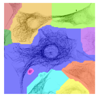
(a) Multi-Xist

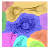
(b) Spectral clustering

Figure 2: Image segmentation of microtubules in NIH 3T3 cells. The colors visualize the resulting $k=10$ partitions via Multi-Xist and spectral clustering, respectively. The underlying cell clusters are visible in black, where a darker color marks denser microtubule network.

We see that Multi-Xist does indeed yield a sensible partition, and it is also able to separate neighbouring cell clusters of different scales, correctly separating smaller, more disconnected cell clusters from the rest. This is in contrast to spectral clustering which cuts right through the main cell cluster, separating it into a red and blue part. This example exemplifies also the scalability issues spectral clustering faces when dealing with clusters of different scales [9]. A visualization of the full Multi-Xist process on this image, in particular the selection of which cluster to cut further, is shown in Figure 2, where we let $k=2,\ldots,9$. This example demonstrates even more clearly the multiscale advantage Xist has over spectral clustering can be found in Figure 5 in Section A.1.

4.2 Empirical runtime comparison

We compare the runtime of the basic algorithm and the proposed $\operatorname{\mathrm{Xist}}$ algorithm on the same cell image dataset as in Section 4.1. We crop the images to $504\times 504$ and vary the “resolution” of the grid (i.e. the grid size parameter $r$) and examine the rates at which the runtime increases, see Figure 3.

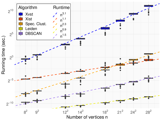
Figure 3: Comparison of the empirical runtimes (in seconds) of the basic Xvst algorithm (blue), Xist (red), spectral clustering (orange), DBSCAN (purple) and Leiden (yellow) on a $\log$-$\log$ scale against the number $n=r^{2}$ of vertices, with dashed lines indicating the empirical complexity of the respective algorithms. The boxplots were obtained by applying each algorithm to a dataset of 21 NIH3T3 cell cluster images of size $504\times 504$ pixels each after discretizing it onto a $r\times r$ grid, for $r\in\{8,9,12,14,18,21,24,28,36,48\}$.

As is shown, the proposed Xist algorithm is empirically roughly two orders of magnitude faster than the basic Xvst algorithm. As the grid size increases, it also becomes faster than spectral clustering (as implemented in the sClust R package). Still, DBCSAN and the Leiden algorithm outperform Xist in terms of raw time, but this is mainly due to their fast implementation – both are realized as C++ routines in their respective R packages: DBSCAN in dbscan and Leiden in igraph (or, alternatively, leiden). We are currently in the process of implementing Xist efficiently (i.e. in C++).

4.3 Qualitative assessment of Xist

We consider two scenarios and compare the proposed Xist algorithm to three well-established (graph) clustering algorithms.

• the classical spectral clustering approach originally proposed by [39], where the eigenvector entries are clustered again using $k$-means clustering, see [44, section 4];

• the Leiden algorithm introduced by [42];

• DBSCAN, originally proposed by [10].

While the Xist algorithm and spectral clustering always output two partitions, the same cannot be said for the other two algorithms, both of which use an additional input: The Leiden algorithm requires a resolution parameter, and DBSCAN has a distance parameter. For both methods, the parameter is hand-tuned to give the minimal classification error or NCut value, respectively; see Figure 4. Such choices of parameters require the knowledge of the true cluster assignments, thus referred to as oracle parameter choices.

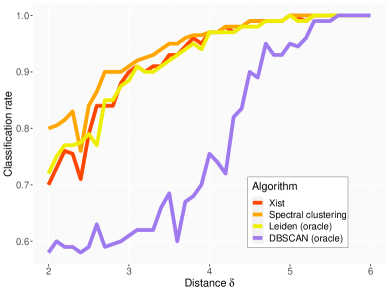
(a) NCut value

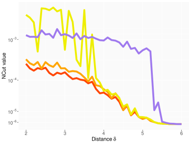
(b) Classification rate

Figure 4: Comparison of the classification rate and NCut value of Xist (red), spectral clustering (orange), Leiden oracle (yellow) and DBSCAN oracle (violet) over the intercluster distance $\delta$. The graph used in the first three algorithms is built out of the sample ${\boldsymbol{X}}$ of $n=100$ points using a combination of 5-nearest and 0.2-neighbourhood, i.e. by defining $\{u,v\}\in E$ if and only if $u\in\mathrm{NN}_{5}(v)$ or $v\in\mathrm{NN}_{5}(u)$ or $\left\lVert u-v\right\rVert\leq 0.2$, where $\mathrm{NN}_{5}(u)$ denotes the set of five nearest (in terms of the euclidean norm $\left\lVert\cdot\right\rVert$ on $\mathbb{R}^{2}$) neighbours in $V$ of $u\in V$. The weights are defined as $w_{uv}\coloneqq\exp(-\left\lVert u-v\right\rVert/0.2)$. These choices are made to ensure a connected graph (5-nearest neighbours) where clusters are more easily detectable (0.2-neighbourhood) and the spatial structure is pronounced (exponential weights). The curves depicted where obtained by taking the mean classification rate and mean NCut value over $100$ iterations of the above procedure, re-generating ${\boldsymbol{X}}$ each time.

It should also be noted that DBSCAN is the only algorithm that does not require an underlying graph structure. Naturally, this makes comparison difficult, especially since the construction of the graph greatly influences the resulting clustering as we will see in the following. The first task to evaluate the quality of our algorithm is that of cluster detection, more precisely, to determine whether a given distribution is constituted by one or two clusters. To this end let $\delta>0$ and consider a random mixture of Gaussians:

$${\boldsymbol{X}}\coloneqq(X_{1},\ldots,X_{n})\sim BZ_{0}+(1-B)Z_{\delta},$$

where $B\sim\mathrm{Ber}(\tfrac{1}{2})$ a Bernoulli random variable, and $Z_{\delta}\sim\mathcal{N}_{2}({\boldsymbol{\delta}},{\boldsymbol{I}}_{2})$ the two-dimensional standard Gaussian around ${\boldsymbol{\delta}}=(\delta,\delta)\in\mathbb{R}^{2}$. For details on the graph construction see Figure 4. [24] have shown that in this scenario (i.e. random mixture of Gaussians), spectral clustering is minimax optimal, so this serves as a benchmark as we cannot hope to outperform it in terms of classification rate (i.e. the ratio of observations $X_{i}$ correctly classified as belonging to their respective Gaussian in the mixture). Despite this, Xist is able to achieve a similar accuracy to the Leiden algorithm, being only slightly worse than spectral clustering. To elaborate, consider Figure 4 (a), where the classification rate is plotted over the intercluster distance $\delta$. Note that, as stated before, both Leiden and DBSCAN were realized as an oracle, i.e. they output the classification rate in (a) and lowest NCut value in (b) over a range of their respective tuning parameter. Still, both are consistently outperformed by Xist and spectral clustering, especially in Figure 4 (b), where Xist yields a consistently better NCut value than all three other algorithms, thus achieving its set goal of approximating graph cuts better than spectral clustering in particular.

4.4 Clustering large network datasets

To demonstrate the applicability and versatility of Xist, even in its current R implementation, we take on the task of clustering large network datasets. We consider the “Stanford Large Dataset Collection” (SNAP, see [22]) which contains many real-world network graphs of varying types and sizes. Of those graphs we consider several undirected graphs, all unweighted, in particular

• the arXiv High-Energy Physics – Phenomenology (HEP-PH) dataset [21, 14] where authors represent nodes and edges papers co-authored between them;

• parts of the Multi-Scale Attributed Node Embedding (MUSAE) dataset [35], namely

  • the MUSAE Facebook subset, where nodes are verified Facebook pages and edges mutual links between them;

  • the MUSAE Squirrel subset, where nodes are squirrel-related Wikipedia pages and edges mutual links between them;

• the Artist subset of the GEMSEC Facebook dataset [36], consisting of nodes representing verified Facebook pages categorized as “artist” and edges mutual likes between them;

• the Enron email dataset [23, 20], containing Enron email addresses as nodes and edges between nodes if an email was sent from one node to the other;

• and the Twitch Gamers dataset [37], where vertices are Twitch users and edges are defined between users who mutually follow each other.

In all datasets, node features were ignored as the algorithms in question are not designed to account for such information. Also note that the selection of subsets of these datasets was essentially arbitrary; similar results hold for other subsets (e.g. the MUSAE crocodile subset).

On the above datasets, we compare the performance of Xist and the Leiden algorithm. Note that DBSCAN is not applicable here since it is a point clustering algorithm, and that spectral clustering cannot be reasonably applied here since it requires computation of the eigenvalues of the graph Laplacian, an $n\times n$ matrix, a task that is very memory-intensive. In our current R implementation of spectral clustering, even partitioning the NIH 3T3 cell images of Section 4.1 (see Figure 2, for instance), takes more than an hour. Consequently, as we consider datasets with tens or hundreds of thousands of nodes, we only compare Xist with the Leiden algorithm, both in terms of the Normalized Cut value of the partition as well as the time the algorithms take. The result can be found in Table 2.

Table 2: Normalized Cut value and empirical runtime of Xist and the Leiden oracle for various datasets. Here, $n$ and $m$ are the number of vertices and edges of only the largest connected component of the respective dataset.

			NCut value		Time
Dataset	$n$	$m$	$\operatorname{\mathrm{Xist}}$	Leiden	$\operatorname{\mathrm{Xist}}$	Leiden
arXiv HepPh	11204	117619	$1.01\cdot 10^{-8}$	$1.01\cdot 10^{-8}$	$54.35$s	$0.46$s
MUSAE Squirrel	5201	198353	$2.61\cdot 10^{-7}$	$5.40\cdot 10^{-7}$	$38.61$s	$0.49$s
MUSAE Facebook	22470	170823	$3.01\cdot 10^{-8}$	$3.08\cdot 10^{-8}$	$165.12$s	$0.45$s
GEMSEC Facebook Artist	50515	819090	$4.70\cdot 10^{-8}$	$4.70\cdot 10^{-8}$	$1461.34$s	$2.82$s
Enron Email	33696	180811	$1.25\cdot 10^{-8}$	$1.28\cdot 10^{-8}$	$212.10$s	$0.43$s
Twitch Gamers	168114	6797557	$7.28\cdot 10^{-8}$	$4.29\cdot 10^{-7}$	$18.23$h	$0.20$h

There are several things to note here. Firstly, we restricted the original datasets to only their largest respective components since, as previously mentioned, Xist would immediately separate unconnected components and return an XCut value of $0$ (for any XCut balancing term). Secondly, as the Leiden algorithm requires a resolution parameter, we consider it as an oracle here, where we choose the parameter that minimizes the XCut value of the partition that Leiden returns. Since Leiden yields a partition of the graph into $k$ sets of vertices, where $k$ is heavily dependent upon the resolution parameter, it is necessary to generalize the XCut term $\operatorname{\mathrm{XC}}$ to a $k$-fold partition of $G$. This generalization is well-established in the literature, and it is given by

$$\operatorname{\mathrm{XC}}_{T}(G) :=\frac{1}{2}\sum_{i=1}^{k}\operatorname{\mathrm{XC}}_{T_{i}}(G)$$

$$\text{for}\quad T =\{T_{1},\ldots,T_{k}\}\subset V^{k}\text{ with }\sum_{i=1}^{k}T_{i}=V$$

(and all $T_{i}$ are pairwise disjoint). Compared to the original definition of $\operatorname{\mathrm{XC}}_{S}(G)$, where $S\subset V$, it is evident that $\operatorname{\mathrm{XC}}_{S}(G)=\operatorname{\mathrm{XC}}_{\{S,{S}^{\mathsf{c}}\}}(G)$.

Returning to Table 2, it is evident that Xist is able to handle large datasets, even though it takes much longer than the Leiden oracle. Note that the times of the oracle do not include the selection process of the resolution parameter as this search can be made to last arbitrarily long by extending the search interval or decreasing the distance between consecutive parameters in consideration. Additionally, as previously stated, Xist is only implemented in R (whereas Leiden has a C++ implementation), and, for the above datasets, the empirical bottleneck of Xist was the computation of the local maxima, an operation which is not a bottleneck theoretically (see Theorem 3.2). Consequently, the times should be interpreted very cautiously.

Qualitatively, it is evident that Xist yields a partition with equal or lower NCut value than Leiden, even though the latter is treated as an oracle that minimizes the NCut value, where the minimization runs over suitable resolution parameters; here, from $10^{-6}$ to $10^{-4}$. Outside of this interval, Leiden returns either only one cluster or too many to minimize the ($k$-fold) NCut value. This suggests that Xist provides a better approximation of NCut than even the Leiden oracle specifically set up to optimize the NCut value.

5 Conclusion and discussion

In the article, we have proposed a novel algorithm Xist for balanced graph cuts, which preservers the qualitative (multiscale) feature of the original graph cut and meanwhile allows fast computation even for large scale datasets, in particular for sparse graphs. This is achieved by combining the combinatorial nature of $st$-MinCuts with the acceleration techniques based on restriction to vertices of locally maximal degrees and vertex merging.

We have demonstrated the applicability and versatility of our algorithm on (cell) image segmentation, simulated data as well as large network datasets. The desirable performance of the proposed Xist, also seen from our simulations, benefits greatly from the structure of $\operatorname{V^{\mathrm{loc}}}$, induced by locally maximizing the degree, and its ordering, which respects the intrinsic geometric structure of the data, to a large extent. We stress, however, that the theoretical findings of Theorem 3.1, in particular its guarantee to consider $|\operatorname{V^{\mathrm{loc}}}|-1$ distinct partitions, and Theorem 3.2 are applicable to any subset of $V$. This means that Xist can be easily adapted to other interesting subsets of vertices, making the algorithm even more flexible.

Appendix A Appendix

A.1 Further comparison study

Figure 5 is an extension of Figure 2, comparing the Multi-Xist algorithm and spectral clustering on the same cell image example, for different $k\in\{2,\ldots,9\}$. In particular, this exemplifies the selection process of Multi-Xist, namely which subgraph to cut.

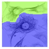
(a) Multi-Xist, $k=2$

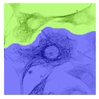
(b) Spec. clust., $k=2$

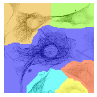
(i) Multi-Xist, $k=6$

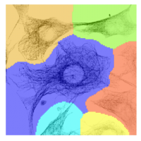
(j) Spec. clust., $k=6$

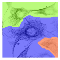
(c) Multi-Xist, $k=3$

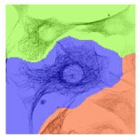
(d) Spec. clust., $k=3$

(k) Multi-Xist, $k=7$

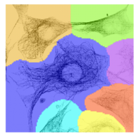
(l) Spec. clust., $k=7$

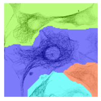
(e) Multi-Xist, $k=4$

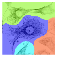
(f) Spec. clust., $k=4$

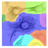
(m) Multi-Xist, $k=8$

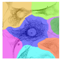
(n) Spec. clust., $k=8$

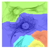
(g) Multi-Xist, $k=5$

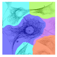
(h) Spec. clust., $k=5$

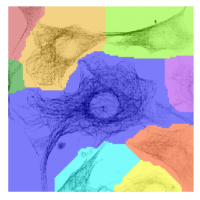
(o) Multi-Xist, $k=9$

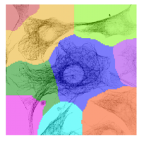
(p) Spec. clust., $k=9$

Figure 5: Extension of Figure 2 on image segmentation of microtubules in NIH 3T3 cells. The colors visualize the resulting $k\in\{2,\ldots,9\}$ partitions via Multi-Xist and spectral clustering, and the underlying cell clusters are visible in black. The case $k=10$ is depicted in Figure 2.

A.2 Correctness of Xist

In the following we present a proof for the correctness of our algorithms as previously claimed in Theorem 3.1. As seen in the proof of this theorem, Xist and the basic Xvst algorithm yield the same output under Assumption 1. Here, we show the remaining claim, namely that Xist outputs $\min_{s,t\in\operatorname{V^{\mathrm{loc}}}}\operatorname{\mathrm{XC}}_{S_{st}}(G)$. Clearly, by definition of Xist (specifically lines 2-2), we are only left to show that through the selection method via $\tau$, $st$-MinCuts for all pairs $s,t\in A:=\operatorname{V^{\mathrm{loc}}}$ are considered.

We start with some preliminary results. The first of these statements and their proofs are due to [15], and the overall structure of this section as well as the remaining claims and the proof of Theorem A.5 are adapted from [17], with changes necessary to account for the specific design of Xist and the generalization to only consider vertices from an arbitrary (but fixed) subset $A\subset V$.

Lemma A.1.

For a weighted graph $G=(V,E,{\boldsymbol{W}})$ and any $v_{1},\ldots,v_{k}\in V$, $k\in\mathbb{N}_{\geq 2}$, with $v_{i}\neq v_{i+1}$ for $i\in\{1,\ldots,k-1\}$, denote $c_{ij}:=\operatorname{\mathrm{MC}}_{S_{v_{i}v_{j}}}(G)$. Then

$$c_{1,k}\geq\min\{c_{1,2},c_{2,3},\ldots,c_{k-1,k}\}.$$ (A.1)

Proof.

Suppose the claim does not hold, i.e. $c_{1,k}<c_{i,i+1}$ for all $i=1,\ldots,k-1$. Let $S\subset V$ denote the partition attaining the $v_{1}v_{k}$-MinCut $c_{1,k}$. Then, there exists an $i\in\{1,\ldots,k-1\}$ such that $v_{i}$ and $v_{i+1}$ are on different sides of $S$ (i.e. either $v_{i}\in S$ and $v_{i-1}\in{S}^{\mathsf{c}}$ or vice versa) because $v_{1}\in S$ and $v_{k}\in{S}^{\mathsf{c}}$. Then, for this $i$, the partition attaining $c_{i,i+1}$ is also a valid $v_{1}v_{k}$-cut, and thus, as $c_{1k}$ is the $v_{1}v_{k}$-MinCut value, $c_{1k}\geq c_{i,i+1}$, contradicting the supposition. ∎

Corollary A.2.

For a weighted graph $G=(V,E,{\boldsymbol{W}})$ and pairwise distinct $s,t,v\in V$, $\min\{\operatorname{\mathrm{MC}}_{S_{st}}(G),\operatorname{\mathrm{MC}}_{S_{sv}}(G),\operatorname{\mathrm{MC}}_{S_{vt}}(G)\}$ is not uniquely attained.

The following Lemma A.3 shows that for any two vertices $u,v$ on the same side of an $st$-MinCut there is a $uv$-MinCut that preserves the $st$-MinCut partition by remaining on one side of the cut.

Lemma A.3.

Let $G=(V,E,{\boldsymbol{W}})$ be a weighted graph, let $s,t\in V$, $s\neq t$, and $u,v\in S_{st}$, $u\neq v$. Then, if $t\in{S}^{\mathsf{c}}_{uv}$, $S_{st}\cap S_{uv}$ is a $uv$-MinCut, and if $t\in S_{uv}$, $S_{st}\cap{S}^{\mathsf{c}}_{uv}$ is a $uv$-MinCut.

Proof.

For the $uv$-MinCut partition $S_{uv}$ in $G$, define

$$A_{1} :=S_{st}\cap S_{uv},\quad A_{2}:=S_{st}\cap{S}^{\mathsf{c}}_{uv},$$

$$A_{3} :={S}^{\mathsf{c}}_{st}\cap S_{uv},\quad\text{and }A_{4}:={S}^{\mathsf{c}}_{st}\cap{S}^{\mathsf{c}}_{uv}.$$

W.l.o.g. assume that $s,u\in A_{1}$ (otherwise exchange $u$ and $v$ and/or $A_{1}$ and $A_{3}$), and that $v\in A_{2}$ (otherwise exchange $A_{2}$ and $A_{4}$). For $k,\ell\in\{1,2\}$ define

$$c_{k\ell}:=\sum_{\begin{subarray}{c}i\in A_{k},j\in B_{\ell}\\ \{i,j\}\in E\end{subarray}}w_{ij}.$$

First assume that $t\in A_{3}$. Notice that $A_{2}$ is a valid $uv$-cut in $G$, and that $S_{uv}=A_{1}\cup A_{3}$ is the $uv$-MinCut in $G$, so

$$0 \leq\operatorname{\mathrm{MC}}_{A_{2}}(G)-\operatorname{\mathrm{MC}}_{S_{uv}}(G)$$

$$=(c_{21}+c_{23}+c_{24})-(c_{12}+c_{14}+c_{32}+c_{34})$$

$$=c_{24}-(c_{14}+c_{34})$$ (A.2)

since $c_{k\ell}=c_{\ell k}$ for all $k,\ell=1,2$. Now assume first that $t\in A_{3}$. Then, $A_{3}$ is a valid $st$-cut in $G$, and $S_{st}=A_{1}\cup A_{2}$ is the $st$-MinCut in $G$, so that

$$0 \leq\operatorname{\mathrm{MC}}_{A_{3}}(G)-\operatorname{\mathrm{MC}}_{S_{st}}(G)$$

$$=(c_{31}+c_{32}+c_{34})-(c_{13}+c_{14}+c_{23}+c_{24})$$

$$=c_{34}-(c_{14}+c_{24})$$ (A.3)

Adding (A.2) and (A.3) yields $0\leq-2c_{14}$ and thus $c_{14}=0$. Using (A.2) (or (A.3)) again gives $c_{24}=c_{34}$, so that

$$\operatorname{\mathrm{MC}}_{A_{2}}(G) =c_{21}+c_{23}+c_{24}$$

$$=c_{12}+c_{14}+c_{32}+c_{34}=\operatorname{\mathrm{MC}}_{S_{uv}}(G),$$

i.e. $A_{2}$ also is a $uv$-MinCut in $G$. As $A_{2}$ is not affected by the contraction of ${S}^{\mathsf{c}}_{st}$, the claim follows under the assumption that $t\in A_{3}$.

If, on the other hand, $t\in A_{4}$, we proceed analogously to before: Modify (A.2) by noting that $A_{1}$ is a valid $uv$-cut in $G$, resulting in $0\leq c_{13}-(c_{23}+c_{34})$, and further modify (A.3) by noting that now $A_{4}$ is a valid $st$-cut in $G$, yielding $0\leq c_{34}-(c_{13}+c_{23})$, so that together $c_{34}=0$ and consequently $c_{13}=c_{23}$. Finally, this results in

$$\operatorname{\mathrm{MC}}_{A_{1}}(G) =c_{12}+c_{14}+c_{13}$$

$$=c_{12}+c_{14}+c_{32}+c_{34}=\operatorname{\mathrm{MC}}_{S_{uv}}(G),$$

yielding the claim also in the case of $t\in A_{4}$. ∎

In the following we present a short and direct proof that the Xist algorithm indeed considers $st$-MinCut partitions for all $s,t\in\operatorname{V^{\mathrm{loc}}}$ and, more significantly, that under the mild Assumption 1, the basic Xvst algorithm and Xist yield the same output. To that end we closely follow the proofs of Gusfield [17, Section 2.1], adapting them to our case whenever necessary, in particular to accommodate for the fact that we are interested in the $st$-MinCut partitions (and not only the cut values themselves) and also the fact that we restrict our attention to only a subset $A\subseteq V$ of vertices (which can be arbitrary for the proof, but for our purposes will of course be $\operatorname{V^{\mathrm{loc}}}$).

To build intuition, we can consider the vector $\tau$ in the Xist algorithm as representation of a tree – in fact, in Theorem A.5 it is shown that this is the Gomory-Hu tree. The interpretation is very simple: There is an edge between $i$ and $\tau_{i}$ for every $i=1,\ldots,|A|$, where $A\subseteq V$ is the subset of vertices (on $G=(V,E,{\boldsymbol{W}})$) Xist is applied to, so $\tau$ can be thought of as a tree with branches between $i$ and $\tau_{i}$. In the following we abbreviate $N:=|A|$ and let $A=\{1,\ldots,N\}\subseteq V:=\{1,\ldots,n\}$ to ease notation. Call $u,v\in A$ neighbours at some point in Xist the $uv$-MinCut is computed (i.e. if $v=\tau_{u}$). Further, for any $u,v\in A$, a sequence of neighbours $\overline{uv}:=\{u,v_{1},\ldots,v_{k},v\}$ such that $u=\tau_{v_{1}}$, $v_{k}=\tau_{v}$ and $v_{i}=\tau_{v_{i+1}}\in A$ for all $i=1,\ldots,k-1$, for some $k\leq N$, is called a directed path from $u$ to $v$.

Lemma A.4.

For a weighted graph $G=(V,E,{\boldsymbol{W}})$ apply Xist to an $A\subseteq V$ with $s,t\in A$, $s\neq t$, such that $s$ and $t$ are connected by a directed path $\overline{st}$, and let $v\in A$ be connected by a directed path to $t$ such that $v<u$ for any $u\in\overline{st}\setminus\{t\}$. Then $s\in S_{vt}$ if and only if $v\in\overline{st}$.

Proof.

At the beginning of Xist, $\tau_{s}=1$, and, from iterations $2$ to $s-1$ in line 2, $\tau_{s}$ changes from one $j$ to one $\ell$, $j,\ell\in\{1,\ldots,N\}$, if and only if (between iterations $2$ and $i-1$) $j$ and $\ell$ were neighbours (i.e. the cut between $j$ and $\tau_{j}=\ell$ is computed at some point throughout Xist). Consequently, a node $j\in A$ was a neighbour of $s$ at some point if and only if $j\in\overline{1s}$. As $t<v$, $v$ must have been a neighbour of $s$ before computation of the $vt$-cut. Moreover, as $v<u$ for any $u\in\overline{st}\setminus\{t\}$, $t$ is a neighbour of $s$ throughout the computation of the $vt$-MinCut (with partition $S_{vt}$). Thus, if $v\in\overline{st}$, $s\in S_{vt}$, and $s\notin S_{vt}$ otherwise. ∎

Theorem A.5.

For a weighted graph $G=(V,E,{\boldsymbol{W}})$ and any subset $A\subseteq V$, Xist applied to $G$ and $A$ considers $st$-MinCuts for all pairs $s,t\in A$.

Proof.

First, note that for each $i=2,\ldots,N$, Xist computes an $i\tau_{i}$-MinCut since always $\tau_{i}<i$ holds, and thus, after an $i\tau_{i}$-MinCut is computed in step $i$, $\tau_{i}$ is not changed afterwards.

Let now $s,t\in A$, $s\neq t$, be arbitrary, and, depending on the context, consider the (directed) path $\overline{st}$ either as a sequence of vertices $s,v_{1},\ldots,v_{k},t$ or edges $(s,v_{1}),(v_{1},v_{2}),\ldots,(v_{k-1},v_{k}),(v_{k},t)$. Abbreviating $c_{uv}:=\operatorname{\mathrm{MC}}_{S_{uv}}(G)$ and $C_{uv}:=\{c_{ij}\mid(i,j)\in\overline{uv}\}$ (for any $u,v\in V$, $u\neq v$), we will show that

$$c_{st}=\min C_{st}$$

which yields the claim immediately because Xist computes all cuts in $\overline{st}$. By Lemma A.1, “$\geq$” holds. For the opposite direction, suppose that “$\leq$” does not hold, and let $s,t\in A$, $s\neq t$, be the vertices forming the shortest path in $\tau$ with this property, i.e. such that $c_{st}>\min C_{st}$.

First, assume that $s$ and $t$ are connected by a directed path in $\tau$, i.e. $s=\tau_{v_{1}}$, $v_{k}=\tau_{t}$ and $v_{i}=\tau_{v_{i}+1}$ for all $i=1,\ldots,k-1$. As the case $k=0$ was tackled in the beginning of this proof, $v:=v_{k}\in A\setminus\{s,t\}$. Due to $\overline{st}$ being minimal (and Lemma A.1), $c_{sv}=\min C_{sv}$, so $c_{sv}=c_{vt}=\min C_{st}$ by Corollary A.2 and the supposition that $c_{st}>\min C_{st}$. However, by Lemma A.4, $S_{vt}$ is also a valid $st$-cut, so $c_{st}\leq c_{vt}=\min C_{st}$, leading to a contradiction.

Second, we tackle the case where $s$ and $t$ are not connected by a directed path, but rather that there is an $r\in A$ such that $\overline{sr}$ and $\overline{rt}$ each form a directed path in $\tau$. As by the first case, $c_{sr}=\min C_{sr}$ and $c_{rt}=\min C_{rt}$ and thus, again, by Corollary A.2 and the supposition we have $c_{sr}=c_{rt}=\min C_{st}=\min C_{sr}\cup C_{rt}$. Define $(u,v)\in\overline{sr}$ to be the vertices closest to $r$ with $c_{uv}=\min C_{sr}=c_{sr}$. By Lemma A.4, $s\in S_{uv}$ and, since $c_{st}>\min C_{st}=\min C_{sr}$, $t\in S_{uv}$.

Let $r_{1},r_{2}\in A$ such that $(r_{1},r)\in\overline{sr}$ and $(r,r_{2})\in\overline{rt}$. W.l.o.g. assume that Xist computed the $r_{1}r$-MinCut before the $rr_{2}$-MinCut. Then $s,u\in S_{r_{1}r}\cap S_{uv}$, $v\in S_{r_{1}r}\cap{S}^{\mathsf{c}}_{uv}$ and $t\in{S}^{\mathsf{c}}_{r_{1}r}\cap S_{uv}$. We can now apply Lemma A.3 to the cuts $S_{r_{1}r}$ and $S_{uv}$. This leads to two cases: If $r\in S_{uv}$, $S_{r_{1}r}\cap S_{uv}$ forms an $uv$-MinCut that is also a valid $vr$-cut, and if $r\in{S}^{\mathsf{c}}_{uv}$, $S_{r_{1}r}\cap{S}^{\mathsf{c}}_{uv}$ constitutes an $uv$-MinCut that is also a valid $st$-cut. In the second case, by definition of $u$ and $v$, $c_{st}\leq c_{uv}=\min C_{st}$, showing the claim. In the first case, $c_{vr}\leq\min C_{st}$, but, since $v$ and $r$ are connected by a directed path in $\tau$, by the above considerations $c_{vr}=\min C_{vr}$ as well as $\min C_{vr}>\min C_{st}$ since $(u,v)$ was the closest pair to $r$ that attains the minimum $\min C_{st}$. Together, $c_{vr}>\min C_{st}$, though this immediately contradicts the definition of $(u,v)$, finishing the proof. ∎

A.3 Proof of Theorem 3.2

Proof.

Since an entry $w_{ij}$ of ${\boldsymbol{W}}$ is zero if $\{i,j\}\not\in E$, we only need $V$ stored as a list (or a self-balancing binary search tree), and ${\boldsymbol{W}}$ stored as an array, as input for the basic Xvst algorithm and Xist. We first analyze Xist line by line:

1. $\mathcal{O}(1)$ computations.

2. Determining $\operatorname{V^{\mathrm{loc}}}$ requires computing the degree of every vertex and determining the local maxima. This can be done simultaneously, and takes at most $n^{2}$ additions and $n-1$ comparisons while taking $\mathcal{O}(n^{2})$ time.

3. Determining $N$ takes $\mathcal{O}(N)$ computations, but only determining whether the algorithm terminates here requires only $\mathcal{O}(1)$ computations.

4. $\mathcal{O}(N)$ runtime due to the creation of $\tau$.

5. Because of line 2 the following steps are executed exactly $N-1$ times:

   1. $\mathcal{O}(1)$ computations.

   2. Orlin’s algorithm [32] for computing an $st$-MinCut partition (by solving the dual problem of computing a max flow from $s$ to $t$) takes $\mathcal{O}(nm+m^{31/16}\log^{2}n)$, which can be reduced for specific types of graphs, e.g. $m=\mathcal{O}(n)$ yields $\mathcal{O}(n^{2}/\log(n))$. If $m=\Omega(n^{1+\varepsilon})$, [19] provided an $\mathcal{O}(nm)$ algorithm which was recently improved by [33] who obtained $\mathcal{O}\Bigl{(}\tfrac{nm\log n}{\log\log n+\log\tfrac{m}{n}}\Bigr{)}$ for $m\geq n$. Thus, by [19, 32, 33], an $st$-MinCut partition can be computed in $\mathcal{O}(nm)$ time for all possible values of $m$ and $n$.

   3. By assumption, the computation time of the XC value for partition ${S}^{\mathsf{c}}_{st}$ is $\mathcal{O}(\kappa)$.

   4. $\mathcal{O}(1)$ computations.

   5. Iterating through all $j=1,\ldots,N$ takes $\mathcal{O}(N)$, and for each $j$, only $\mathcal{O}(1)$ computations are done, yielding $\mathcal{O}(N)$ in total.

Therefore, Xist runs in $\mathcal{O}(N\max\{nm,\kappa\})$ time for general $m$, and in $\mathcal{O}(N\max\{n^{2}/\log n,\kappa\})$ time for $m=\mathcal{O}(n)$ by utilizing [32] as noted above. As the basic Xvst algorithm iterates over all pairs of vertices in $V$ in lines 1 to 1, to ascertain its complexity we simply substitute $N$ by $n^{2}$ to obtain $\mathcal{O}(n^{2}\max\{nm,\kappa\})$. ∎

References

- [1]
- Bonsma [2010] Paul Bonsma. 2010. Most balanced minimum cuts. Discrete Appl. Math. 158, 4 (2010), 261–276. https://doi.org/10.1016/j.dam.2009.09.010
- Bui and Jones [1992] Thang Nguyen Bui and Curt Jones. 1992. Finding good approximate vertex and edge partitions is NP-hard. Inform. Process. Lett. 42, 3 (1992), 153 – 159. https://doi.org/10.1016/0020-0190(92)90140-Q
- Cheeger [1969] Jeff Cheeger. 1969. A lower bound for the smallest eigenvalue of the Laplacian. In Proceedings of the Princeton conference in honor of Professor S. Bochner. 195–199.
- Chen et al. [2011] Wen-Yen Chen, Yangqiu Song, Hongjie Bai, Chih-Jen Lin, and Edward Y. Chang. 2011. Parallel Spectral Clustering in Distributed Systems. IEEE Transactions on Pattern Analysis and Machine Intelligence 33, 3 (2011), 568–586. https://doi.org/10.1109/TPAMI.2010.88
- Chew and Cahill [2015] Selene E. Chew and Nathan D. Cahill. 2015. Semi-Supervised Normalized Cuts for Image Segmentation. In 2015 IEEE International Conference on Computer Vision (ICCV). 1716–1723. https://doi.org/10.1109/ICCV.2015.200
- Chimani et al. [2007] Markus Chimani, Carsten Gutwenger, and Petra Mutzel. 2007. On the minimum cut of planarizations. In 6th Czech-Slovak International Symposium on Combinatorics, Graph Theory, Algorithms and Applications. Electron. Notes Discrete Math., Vol. 28. Elsevier Sci. B. V., Amsterdam, 177–184. https://doi.org/10.1016/j.endm.2007.01.036
- Cook et al. [1998] William Cook, William H. Cunningham, William R. Pulleyblank, and Alexander Schrijver. 1998. Minimum cuts in undirected graphs. John Wiley & Sons, Chapter 3.5, 71–84. https://doi.org/10.1002/9781118033142.ch3
- Dahlhaus et al. [1994] E. Dahlhaus, D. S. Johnson, C. H. Papadimitriou, P. D. Seymour, and M. Yannakakis. 1994. The complexity of multiterminal cuts. SIAM J. Comput. 23, 4 (1994), 864–894. https://doi.org/10.1137/S0097539792225297
- Ester et al. [1996] Martin Ester, Hans-Peter Kriegel, Jörg Sander, and Xiaowei Xu. 1996. A Density-Based Algorithm for Discovering Clusters in Large Spatial Databases with Noise. In Proceedings of the Second International Conference on Knowledge Discovery and Data Mining (Portland, Oregon) (KDD’96). AAAI Press, 226–231.
- García Trillos and Slepčev [2018] Nicolás García Trillos and Dejan Slepčev. 2018. A variational approach to the consistency of spectral clustering. Applied and Computational Harmonic Analysis 45, 2 (2018), 239–281. https://doi.org/10.1016/j.acha.2016.09.003
- Garey and Johnson [1979] Michael R. Garey and David S. Johnson. 1979. Computers and Intractability. W.H. Freeman and Company.
- Gawrychowski et al. [2020] Paweł Gawrychowski, Shay Mozes, and Oren Weimann. 2020. Minimum cut in O(m log² n) time. In 47th International Colloquium on Automata, Languages, and Programming (ICALP 2020) (Leibniz International Proceedings in Informatics (LIPIcs)), Artur Czumaj, Anuj Dawar, and Emanuela Merelli (Eds.), Vol. 168. Schloss Dagstuhl–Leibniz-Zentrum für Informatik, Dagstuhl, Germany, 57:1–57:15. https://doi.org/10.4230/LIPIcs.ICALP.2020.57
- Gehrke et al. [2003] Johannes Gehrke, Paul Ginsparg, and Jon Kleinberg. 2003. Overview of the 2003 KDD Cup. SIGKDD Explor. Newsl. 5, 2 (dec 2003), 149–151. https://doi.org/10.1145/980972.980992
- Gomory and Hu [1961] R. E. Gomory and T. C. Hu. 1961. Multi-terminal network flows. J. Soc. Indust. Appl. Math. 9 (1961), 551–570.
- Guattery and Miller [1998] Stephen Guattery and Gary L. Miller. 1998. On the quality of spectral separators. SIAM J. Matrix Anal. Appl. 19, 3 (07 1998), 701–719.
- Gusfield [1990] Dan Gusfield. 1990. Very simple methods for all pairs network flow analysis. SIAM J. Comput. 19, 1 (1990), 143–155. https://doi.org/10.1137/0219009
- Hagen and Kahng [1992] Lars Hagen and Andrew B. Kahng. 1992. A new approach to effective circuit clustering. In Proceedings of the 1992 IEEE/ACM International Conference on Computer-Aided Design (ICCAD ’92). IEEE Computer Society Press, 422–427.
- King et al. [1994] V. King, S. Rao, and R. Tarjan. 1994. A faster deterministic maximum flow algorithm. J. Algorithms 17, 3 (1994), 447–474. https://doi.org/10.1006/jagm.1994.1044 Third Annual ACM-SIAM Symposium on Discrete Algorithms (Orlando, FL, 1992).
- Klimt and Yang [2004] Bryan Klimt and Yiming Yang. 2004. Introducing the Enron Corpus. https://www.ceas.cc/papers-2004/168.pdf
- Leskovec et al. [2005] Jure Leskovec, Jon Kleinberg, and Christos Faloutsos. 2005. Graphs over Time: Densification Laws, Shrinking Diameters and Possible Explanations. In Proceedings of the Eleventh ACM SIGKDD International Conference on Knowledge Discovery in Data Mining (Chicago, Illinois, USA) (KDD ’05). Association for Computing Machinery, New York, NY, USA, 177–187. https://doi.org/10.1145/1081870.1081893
- Leskovec and Krevl [2014] Jure Leskovec and Andrej Krevl. 2014. SNAP Datasets: Stanford Large Network Dataset Collection. https://snap.stanford.edu/data.
- Leskovec et al. [2009] Jure Leskovec, Kevin J. Lang, Anirban Dasgupta, and Michael W. Mahoney. 2009. Community Structure in Large Networks: Natural Cluster Sizes and the Absence of Large Well-Defined Clusters. Internet Mathematics 6, 1 (2009), 29–123. https://doi.org/10.1080/15427951.2009.10129177
- Löffler et al. [2021] Matthias Löffler, Anderson Y. Zhang, and Harrison H. Zhou. 2021. Optimality of spectral clustering in the Gaussian mixture model. Ann. Statist. 49, 5 (2021), 2506–2530. https://doi.org/10.1214/20-aos2044
- Maier et al. [2013] Markus Maier, Ulrike von Luxburg, and Matthias Hein. 2013. How the result of graph clustering methods depends on the construction of the graph. ESAIM: PS 17 (2013), 370–418. https://doi.org/10.1051/ps/2012001
- Malioutov and Barzilay [2006] Igor Malioutov and Regina Barzilay. 2006. Minimum Cut Model for Spoken Lecture Segmentation. In Proceedings of the 21st International Conference on Computational Linguistics and 44th Annual Meeting of the Association for Computational Linguistics. Association for Computational Linguistics, Sydney, Australia, 25–32. https://doi.org/10.3115/1220175.1220179
- Mohar [1989] Bojan Mohar. 1989. Isoperimetric numbers of graphs. Journal of Combinatorial Theory, Series B 47, 3 (1989), 274 – 291. https://doi.org/10.1016/0095-8956(89)90029-4
- Nadler and Galun [2006] Boaz Nadler and Meirav Galun. 2006. Fundamental limitations of spectral clustering. In Advances in Neural Information Processing Systems, B. Schölkopf, J. Platt, and T. Hoffman (Eds.), Vol. 19. MIT Press. https://proceedings.neurips.cc/paper/2006/file/bdb6920adcd0457aa17b53b22963dad9-Paper.pdf
- Nascimento and de Carvalho [2011] Mariá C.V. Nascimento and André C.P.L.F. de Carvalho. 2011. Spectral methods for graph clustering - A survey. European Journal of Operational Research 211, 2 (June 2011), 221–231.
- Ng et al. [2001] Andrew Y. Ng, Michael I. Jordan, and Yair Weiss. 2001. On spectral clustering: analysis and an algorithm. In Proceedings of the 14th International Conference on Neural Information Processing Systems: Natural and Synthetic (Vancouver, British Columbia, Canada) (NIPS’01). MIT Press, Cambridge, MA, USA, 849–856.
- O et al. [2021] Suil O, Yongtang Shi, and Zhenyu Taoqiu. 2021. Sharp upper bounds on the -independence number in graphs with given minimum and maximum degree. Graphs Combin. 37, 2 (2021), 393–408. https://doi.org/10.1007/s00373-020-02244-y
- Orlin [2013] James B. Orlin. 2013. Max flows in O(nm) time, or better. In Proceedings of the Forty-Fifth Annual ACM Symposium on Theory of Computing (STOC ’13). Association for Computing Machinery, New York, NY, USA, 765–774. https://doi.org/10.1145/2488608.2488705
- Orlin and Gong [2021] James B. Orlin and Xiao-yue Gong. 2021. A fast maximum flow algorithm. Networks 77, 2 (2021), 287–321. https://doi.org/10.1002/net.22001
- Peng et al. [2014] Yi Peng, Li Chen, Fang-Xin Ou-Yang, Wei Chen, and Jun-Hai Yong. 2014. JF-Cut: A Parallel Graph Cut Approach for Large Scale Image and Video. IEEE transactions on image processing : a publication of the IEEE Signal Processing Society 24 (12 2014).
- Rozemberczki et al. [2021] Benedek Rozemberczki, Carl Allen, and Rik Sarkar. 2021. Multi-Scale attributed node embedding. Journal of Complex Networks 9, 2 (05 2021), cnab014. https://doi.org/10.1093/comnet/cnab014 arXiv:https://academic.oup.com/comnet/article-pdf/9/2/cnab014/40435146/cnab014.pdf
- Rozemberczki et al. [2019] Benedek Rozemberczki, Ryan Davies, Rik Sarkar, and Charles Sutton. 2019. GEMSEC: Graph Embedding with Self Clustering. In Proceedings of the 2019 IEEE/ACM International Conference on Advances in Social Networks Analysis and Mining 2019. ACM, 65–72.
- Rozemberczki and Sarkar [2021] Benedek Rozemberczki and Rik Sarkar. 2021. Twitch Gamers: a Dataset for Evaluating Proximity Preserving and Structural Role-based Node Embeddings. arXiv:cs.SI/2101.03091
- Senthilnath et al. [2014] J. Senthilnath, S. Sindhu, and S. N. Omkar. 2014. GPU-based normalized cuts for road extraction using satellite imagery. Journal of Earth System Science 123, 8 (01 Dec 2014), 1759–1769. https://doi.org/10.1007/s12040-014-0513-1
- Shi and Malik [2000] Jianbo Shi and J. Malik. 2000. Normalized cuts and image segmentation. IEEE Transactions on Pattern Analysis and Machine Intelligence 22, 8 (08 2000), 888–905. https://doi.org/10.1109/34.868688
- Šíma and Schaeffer [2006] Jiří Šíma and Satu Elisa Schaeffer. 2006. On the NP-completeness of some graph cluster measures. In Proceedings of the 32nd Conference on Current Trends in Theory and Practice of Computer Science (Měřín, Czech Republic) (SOFSEM’06). Springer-Verlag, Berlin, Heidelberg, 530–537. https://doi.org/10.1007/11611257_51
- Tang et al. [2016] Meng Tang, Dmitrii Marin, Ismail Ben Ayed, and Yuri Boykov. 2016. Normalized Cut Meets MRF. In Computer Vision – ECCV 2016, Bastian Leibe, Jiri Matas, Nicu Sebe, and Max Welling (Eds.). Springer International Publishing, Cham, 748–765.
- Traag et al. [2019] V. A. Traag, L. Waltman, and N. J. van Eck. 2019. From Louvain to Leiden: guaranteeing well-connected communities. Scientific Reports 9, 1 (26 Mar 2019), 5233. https://doi.org/10.1038/s41598-019-41695-z
- van den Heuvel et al. [2008] Martijn van den Heuvel, Rene Mandl, and Hilleke Hulshoff Pol. 2008. Normalized cut group clustering of resting-state FMRI data. PLoS One 3, 4 (April 2008), e2001.
- von Luxburg [2007] Ulrike von Luxburg. 2007. A tutorial on spectral clustering. Statistics and Computing 17 (08 2007), 395–416. https://doi.org/10.1007/s11222-007-9033-z
- von Luxburg et al. [2008] Ulrike von Luxburg, Mikhail Belkin, and Olivier Bousquet. 2008. Consistency of spectral clustering. Ann. Statist. 36, 2 (04 2008), 555–586. https://doi.org/10.1214/009053607000000640
- Wagner and Wagner [1993] Dorothea Wagner and Frank Wagner. 1993. Between min cut and graph bisection. In Proceedings of the 18th International Symposium on Mathematical Foundations of Computer Science (MFCS ’93). Springer-Verlag, Berlin, Heidelberg, 744–750.
- Wang et al. [2020] Faqiang Wang, Cuicui Zhao, Jun Liu, and Haiyang Huang. 2020. A Variational Image Segmentation Model Based on Normalized Cut with Adaptive Similarity and Spatial Regularization. SIAM Journal on Imaging Sciences 13, 2 (2020), 651–684. https://doi.org/10.1137/18M1192366
- Willis [2011] William Willis. 2011. Bounds for the independence number of a graph. Master’s thesis. Virginia Commonwealth University, USA. https://doi.org/10.25772/B95B-C733
- Yu et al. [2016] Miao Yu, Shuhan Shen, and Zhanyi Hu. 2016. Dynamic parallel and distributed graph cuts. IEEE Trans. Image Process. 25, 12 (2016), 5511–5525. https://doi.org/10.1109/TIP.2016.2609819
- Zhong and Pun [2022] G. Zhong and C. Pun. 2022. Improved Normalized Cut for Multi-View Clustering. IEEE Transactions on Pattern Analysis & Machine Intelligence 44, 12 (dec 2022), 10244–10251. https://doi.org/10.1109/TPAMI.2021.3136965