AI Hilbert: A New Paradigm for Scientific Discovery by Unifying Data and Background Knowledge

Abstract

The discovery of scientific formulae that parsimoniously explain natural phenomena and align with existing background theory is a key goal in science. Historically, scientists have derived natural laws by manipulating equations based on existing knowledge, forming new equations, and verifying them experimentally. In recent years, data-driven scientific discovery has emerged as a viable competitor in settings with large amounts of experimental data. Unfortunately, data-driven methods often fail to discover valid laws when data is noisy or scarce. Accordingly, recent works combine regression and reasoning to eliminate formulae inconsistent with background theory. However, the problem of searching over the space of formulae consistent with background theory to find one that fits the data best is not well-solved. We propose a solution to this problem when all axioms and scientific laws are expressible via polynomial equalities and inequalities and argue that our approach is widely applicable. We further model notions of minimal complexity using binary variables and logical constraints, solve polynomial optimization problems via mixed-integer linear or semidefinite optimization, and prove the validity of our scientific discoveries in a principled manner using Positivestellensatz certificates. Remarkably, the optimization techniques leveraged in this paper allow our approach to run in polynomial time with fully correct background theory, or non-deterministic polynomial (NP) time with partially correct background theory. We demonstrate that some famous scientific laws, including Kepler’s Third Law of Planetary Motion, the Hagen-Poiseuille Equation, and the Radiated Gravitational Wave Power equation, can be derived in a principled manner from background axioms and experimental data.

1 Introduction

A fundamental problem in science and engineering involves explaining natural phenomena in a manner consistent with noisy experimental data and a body of potentially inexact and incomplete background knowledge about the universe’s laws de2020understanding . In the past few centuries, The Scientific Method (simon1973does, ) has led to significant progress in discovering new laws. Unfortunately, the rate of emergence of these laws and their contribution to economic growth is stagnating relative to the amount of capital invested in deducing them brynjolfsson2018artificial ; bhattacharya2020stagnation . Indeed, Dirac dirac1978directions noted that it is now more challenging for first-rate physicists to make second-rate discoveries than it was previously for second-rate physicists to make first-rate ones, while Arora et al. arora2018decline found that the marginal value of scientific discoveries to large companies has declined since the fall of the Berlin Wall. This phenomenon can be partly explained by analogy to the work of Cowen cowen2011great , namely, that The Scientific Method has picked most of the “low-hanging fruit” in science and engineering, such as natural laws that relate physical quantities using a small number of low-degree polynomials. This calls for more disciplined and principled alternatives to The Scientific Method, which integrate background information and experimental data to generate and verify higher dimensional laws of nature, thereby promoting scientific discovery (c.f. kitano2021nobel, ; wang2023scientific, ). An overview of such alternatives is depicted in Figure 1.

On the other hand, the past thirty years have seen significant improvements in the scalability of global optimization methods — which, as we argue in this paper, can search over the space of scientific laws — owing to Moore’s law and significant theoretical and computational advances by the optimization community (see bixby2007progress, ; gupta2022branch, ; bertsimas2023matrix, , for reviews). Bertsimas and Dunn (bertsimas2019machine, , Chap. 1) observed that the speedup in raw computing power between $1991$ and $2015$ is at least six orders of magnitude. Additionally, sum-of-squares and polynomial optimization methods have become much more scalable since the work of Parrilo parrilo2003semidefinite , and primal-dual interior-point methods nesterov1994interior have improved considerably, with excellent implementations now available in, for example, the Mosek solver andersen2000mosek .

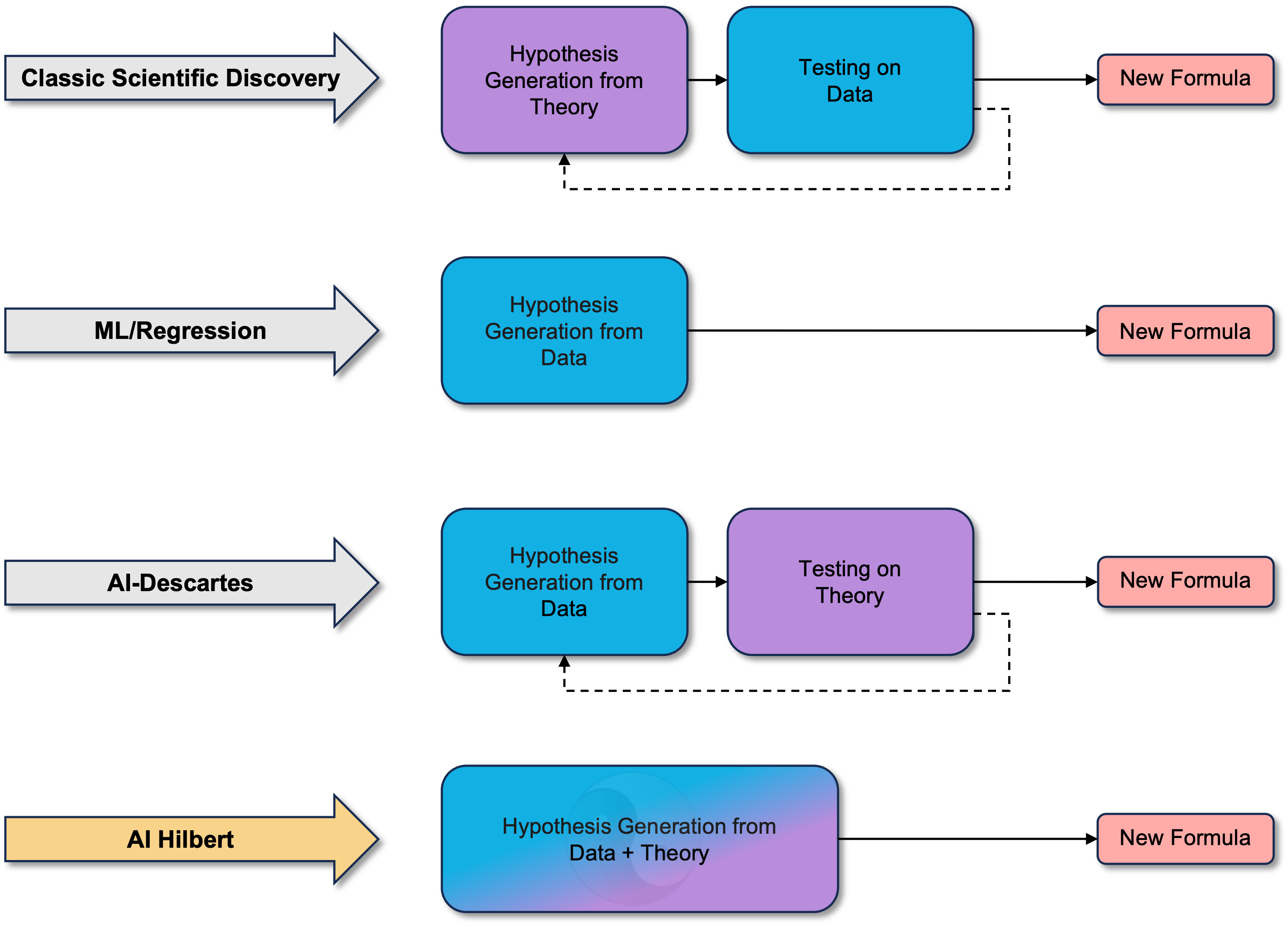
Figure 1: High-level comparison of different scientific method paradigms. Traditional scientific discovery methods formulate hypotheses using existing theory and observed phenomena. These hypotheses are then validated and tested using data. In contrast, machine learning and regression methods primarily rely on large datasets to identify patterns. AI-Descartes cornelio2021ai proposes an inversion of the conventional scientific discovery paradigm. It starts by first generating the hypotheses from observed data (similarly to ML/Regression) and subsequently validating them against the known theory. However, in AI-Descartes, theory and data remain disjoint and do not mutually enhance one another. In contrast, our work, AI Hilbert, combines both data and theory to formulate hypotheses. Unlike conventional methods, both insights in data and knowledge embedded in the theory collaboratively reduce the search space. These two components complement each other: theory compensates for noisy or sparse datasets, while data compensates for theory that is inconsistent or incomplete. Note that blue denotes components associated with data, and purple denotes components linked to theory. Dashed lines represent iterative processes.

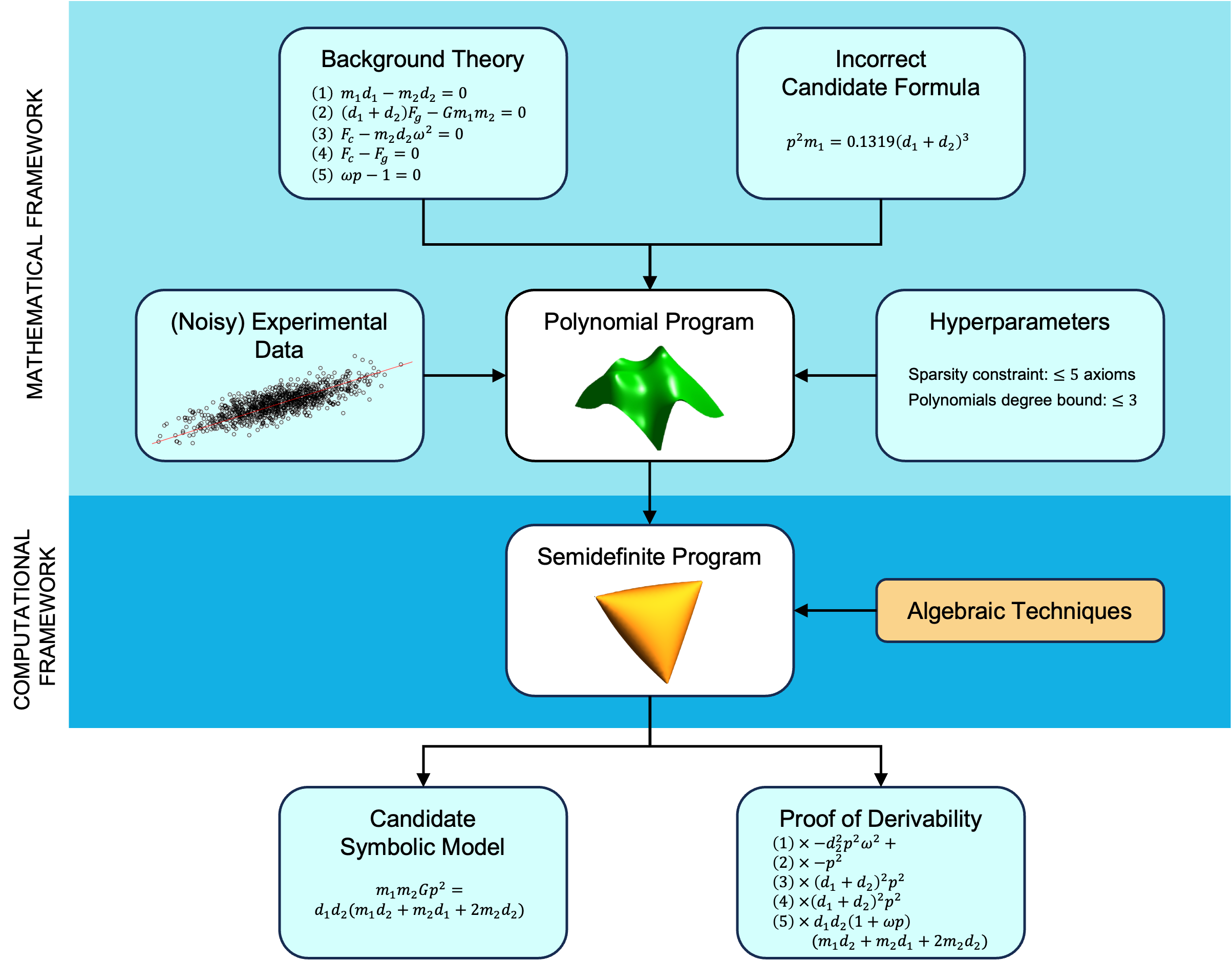
Figure 2: Schematic illustration of discovering Kepler’s third law of planetary motion. Using partially correct background knowledge encoded as multivariate polynomials, experimental data, and a sparsity constraint on the background theory to control our model’s complexity, we formulate scientific discovery as a polynomial optimization problem, reformulate it as a semidefinite optimization problem, and solve to obtain both a symbolic model and its formal derivation.

In this paper, we propose a new approach to scientific discovery that leverages these advances by the optimization community; see Figure 2 for a high-level overview of our approach. Given a set of background axioms, theorems, and laws expressible as a basic semialgebraic set (i.e., a system of polynomial equalities and inequalities) and observations from experimental data, we derive new laws representable as polynomial expressions that are either exactly or approximately consistent with existing laws and experimental data by solving polynomial optimization problems via linear and semidefinite optimization. By leveraging fundamental results from real algebraic geometry, we obtain formal proofs of the correctness of our laws as a byproduct of the optimization problems. This is notable, because existing automated approaches to scientific discovery, as reviewed in Section 1.1, often rely upon deep learning techniques that do not provide formal proofs and are prone to “hallucinating” incorrect scientific laws that cannot be automatically proven or disproven, analogously to output from state-of-the-art Large Language Models such as GPT-$4$ open2023gpt4 . As such, any new laws derived by these systems cannot easily be explained or justified. On the other hand, our approach discovers new scientific laws by solving an optimization problem to minimize a weighted sum of discrepancies between the proposed law and experimental data, plus the distance between the discovered law and its projection onto the set of symbolic laws derivable from background theory. As a result, our approach discovers scientific laws alongside a proof of their consistency with existing background theory by default. Moreover, our approach is scalable; it runs in polynomial time (when the degree of the polynomial certificates we search over is bounded; see Section 2.2) with a complete and correct set of background theory.

We believe our approach could be a first step towards discovering new laws of the universe which involve higher degree polynomials and are impractical for scientists to discover without the aid of modern solvers and high-performance computing environments. Further, our approach is potentially useful for reconciling mutually inconsistent axioms. Indeed, if a system of scientific laws is mutually inconsistent (in the sense that no point satisfies all laws simultaneously), our polynomial optimization problem offers a formal proof of its inconsistency. Moreover, our approach allows scientists to make discoveries using at most $k$ laws out of a supplied list of $n$ laws (where $n>k$), meaning it is possible to select the $k$ laws that best explain the experimental data.

1.1 Literature Review

We propose an approach to scientific discovery, which we term AI-Hilbert, that uses polynomial optimization to obtain scientific formulae derivable from background theory axioms and consistent with experimental data. We remark that this differs from existing works on scientific discovery that sometimes involve expressing prior knowledge as constraints on the functional form of a learned model (e.g., shape constraints such as monotonicity curmei2020shape ). Indeed, shape-constrained approaches to scientific discovery have been proposed (see, e.g., kubalik2020symbolic, ; kubalik2021multi, ; engle2022deterministic, ; curmei2020shape, ; bertsimas2023learning, ), while discovering scientific laws that are simultaneously derivable from prior knowledge expressed as polynomials and experimental data is an open problem.

AI-Hilbert builds upon two areas typically considered in isolation: semidefinite and sum-of-squares optimization techniques for solving polynomial optimization problems, and data-driven techniques for symbolic discovery. We now review the relevant literature.

Sum-of-Squares Optimization:

Sum-of-squares optimization has been an important component of global optimization methods since the seminal work of Parrilo parrilo2003semidefinite (see also Lasserre lasserre2001global ), which combines two key observations. First, sum-of-squares decompositions of multivariate polynomials can be computed via semidefinite optimization, so optimizing over sum-of-squares polynomials is no harder than performing semidefinite optimization. Second, owing to a fundamental result from real algebraic geometry, namely the Positivestellensatz krivine1964anneaux ; stengle1974nullstellensatz ; putinar1993positive , polynomials of bounded degree defined on basic semialgebraic sets can be certified as non-negative over these sets by representing them as systems of sum-of-squares polynomials (see Section 1.3). Consequently, optimizing over a real polynomial system is (under mild assumptions) equivalent to solving a (larger) sum-of-squares optimization problem, and thus a tractable convex problem. These observations have allowed an entire field of optimization to blossom; see Blekherman et al. blekherman2012semidefinite , Hall hall2019engineering for reviews. However, to our knowledge, no works have proposed using sum-of-squares optimization to discover scientific formulae. The closest works are Clegg et al. clegg1996using , who propose using Gröbner bases to design proofs of unsatisfiability, Curmei and Hall curmei2020shape , who propose a sum-of-squares approach to fitting a polynomial to data under very general constraints on the functional form of the polynomial, e.g., non-negativity of the derivative over a box, Ahmadi and El Khadir bachir2023sideinfo , who propose learning the behavior of noisy dynamical systems via semialgebraic techniques, and Fawzi et al. fawzi2019learning , who propose learning proofs of optimality of stable set problems by combining reinforcement learning with the Positivestellensatz. However, determining whether polynomial optimization is practically useful for scientific discovery remains open.

Data-Driven Approaches to Scientific Discovery:

The availability of large amounts of scientific data generated and collected over the past few decades has spurred increasing interest in data-driven methods for scientific discovery that aim to identify symbolic equations that accurately explain high-dimensional datasets. Bongard and Lipson bongard2007automated and Schmidt and Lipson schmidt2009distilling proposed using heuristics and genetic programming to discover scientifically meaningful formulae, and implemented their approach in the Eureqa software system dubvcakova2011eureqa . Other proposed approaches are based on mixed-integer global optimization austel2017globally ; cozad2018global , sparse regression brunton2016discovering ; rudy2017data ; bertsimas2023learning , Cylindrical Algebraic Decomposition fulton2015keymaera , neural networks iten2020discovering ; landajuela2022unified , and Bayesian Markov Chain Monte Carlo approaches guimera2020bayesian . See karagiorgi2022machine ; baum2021artificial for reviews of data-driven scientific discovery in fundamental physics and chemistry.

Data-driven approaches have since been shown by several authors to perform well in highly overdetermined settings with limited amounts of noise. For instance, Udrescu et al. udrescu2020ai ; udrescu2020ai2 proposed a method called AI-Feynman, which combines neural networks with physics-based techniques to discover symbolic formulae. Moreover, they constructed a benchmark dataset of $100$ scientific laws derived from Richard Feynman’s lecture notes feynman1965feynman , with $100,000$ noiseless experimental observations of each scientific law, and demonstrated that while the Eurequa system could recover an already impressive $71/100$ instances from the data, their approach could recover all one hundred; see the work of Cornelio et al. cornelio2021ai for a review of scientific discovery systems.

Unfortunately, data-driven approaches to scientific discovery have at least three significant drawbacks. First, they are not data efficient fujinuma2022big and only reliably recover scientific formulae in highly overdetermined settings with several orders of magnitude more data than a human would likely need to make the same discoveries. Indeed, Matsubara et al. matsubara2022srsd recently argued that the sampling regime used by AI-Feynman is unrealistic, because it samples values far from those observable in the real world. Moreover, Cornelio et al. cornelio2021ai recently rebenchmarked AI-Feyman on $81$ of the $100$ aforementioned laws, but with $10$ (rather than $100,000$) observations per law, and where each experimental observation is contaminated with a small amount of noise. In this limited data setting, Cornelio et al. cornelio2021ai found that AI-Feyman recovered $40$ of the $81$ laws considered, whereas they were able to recover $49/81$ laws using their symbolic regression solver. This performance degradation is a significant issue in practice because scientific data is typically expensive to obtain and scarce and noisy. Second, purely data-driven methods are agnostic to important background information, such as existing literature, that valid scientific formulae should be consistent with unless there is extraordinary experimental evidence that the literature is incorrect. This implies that data-driven methods search over a larger space of laws than is necessary, require more data than a human would need to derive a valid law, and frequently propose laws that are not scientifically meaningful. Third, they typically do not provide interpretable explanations for why their discoveries are valid (c.f. rudin2019stop, ), which makes diagnosing whether their discoveries are consistent with existing theory challenging.

To account for background theory in scientific discovery, Cornelio et al. cornelio2021ai recently proposed an approach called AI-Descartes, which iteratively generates plausible scientific formulae using a mixed-integer nonlinear symbolic regression solver (see also austel2017globally, ), and tests whether these formulae are derivable from the background knowledge. In the case they are not, the method provides a set of reasoning-based measures to compute how distant the formulae induced from the data are from the background theory, but is unable to recover the correct formulae. This is because their approach derives potential scientific laws from data and subsequently tests the hypothesis against the background theory, rather than learning from axioms and data simultaneously.

1.2 Contributions and Structure

We propose a novel automated approach to scientific discovery, which we term AI-Hilbert, that utilizes techniques from the polynomial and sum-of-squares optimization literatures to derive polynomial scientific laws that best explain a set of experimental data while maintaining consistency with a body of background knowledge. Our approach is inspired by the generality of the sum-of-squares optimization framework and the work of David Hilbert, who was one of the first mathematicians to investigate the power and expressivity of sum-of-squares functions of polynomials.

Our approach automatically provides an axiomatic derivation of the correctness of the discovered scientific law derived, conditional on the correctness of our background theory. Moreover, in instances with inconsistent background theory, our approach is capable of successfully identifying the sources of inconsistency by performing best subset selection to determine the axioms which best explain the data. This is notably different from current data-driven approaches to scientific discovery, which often generate spurious laws in limited data settings and fail to differentiate between valid and invalid discoveries, or provide explanations of their derivations. We illustrate our approach by axiomatically deriving some of the most frequently cited natural laws in the scientific literature, including Kepler’s Third Law and Einstein’s Relativistic Time Dilation Law, among other scientific discoveries.

A second contribution of our approach is that it permits fine-grained control of the tractability of the scientific discovery process, by bounding the degree of the coefficients in the Positivestellensatz certificates that are searched over (see Section 1.3, for a formal statement of the Positivestellensatz). This differs from prior work on automated scientific discovery, which offers more limited control over its time complexity. For instance, in the special case of scientific discovery with a complete body of background theory and no experimental data, to our knowledge, the only current alternative to our approach is symbolic regression (see, e.g., cozad2018global, ), which requires genetic programming or mixed-integer nonlinear programming techniques that are not guaranteed to run in polynomial time. On the other hand, our approach searches for polynomial certificates of a bounded degree by leveraging a fixed level of the sum-of-squares hierarchy lasserre2001global ; parrilo2003semidefinite , which can be searched over in polynomial time nesterov1994interior ; ramana1997exact .

To contrast our approach with existing approaches to scientific discovery, Figure 3 depicts a stylized version of the scientific method. In this version, new laws of nature are proposed from background theory (which may be written down by humans, automatically extracted from existing literature, or generated using AI) and experimental data, using classical scientific discovery techniques, data-driven techniques, or AI-Hilbert. Observe that data-driven discoveries may be inconsistent with background theory, and discoveries via classical methods may not be consistent with relevant data sources, while discoveries made via AI-Hilbert are consistent with background theory and relevant data sources. This suggests that AI-Hilbert could be a first step toward scientific discovery frameworks that are less likely to make false discoveries. Moreover, as mentioned in the introduction, AI-Hilbert uses background theory to restrict the effective dimension of the set of possible scientific laws, and, therefore, likely requires less experimental data to make scientific discoveries than purely data-driven approaches.

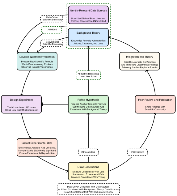
Figure 3: The Scientific Method With Scientific Discoveries Made Via Classical Methods, Data-Driven Methods, or AI-Hilbert. AI-Hilbert proposes scientific laws consistent with a body of background theory formally articulated as polynomial equalities, inequalities, and relevant data sources. This likely allows scientific discoveries to be made using fewer data points than via state-of-the-art approaches, and for missing scientific axioms to be deduced via abductive reasoning as part of the scientific discovery process. On the other hand, existing approaches to scientific discovery propose laws that may be inconsistent with either background theory or existing data sources.

1.3 Background and Notation

The notation is mostly standard to the polynomial optimization literature. We let non-boldface characters such as $b$ denote scalars, lowercase bold-faced characters such as $\bm{x}$ denote vectors, uppercase bold-faced characters such as $\bm{A}$ denote matrices, and calligraphic uppercase characters such as $\mathcal{Z}$ denote sets. We let $[n]$ denote the set of indices $\{1,\dots,n\}$. We let $\bm{e}$ denote the vector of ones, $\bm{0}$ denote the vector of all zeros, and $\mathbb{I}$ denote the identity matrix. We let $\|\bm{x}\|_{p}$ denote the $p$-norm of a vector $\bm{x}$ for $p\geq 1$. We let $\mathbb{R}$ denote the real numbers, $\mathcal{S}^{n}$ denote the cone of $n\times n$ symmetric matrices, and $\mathcal{S}^{n}_{+}$ denote the cone of $n\times n$ positive semidefinite matrices.

We also use some notations specific to the sum-of-squares (SOS) optimization literature; see cox2013ideals for an introduction to computational algebraic geometry and blekherman2012semidefinite for a general theory of sum-of-squares and convex algebraic optimization. Specifically, we let $\mathbb{R}[\bm{x}]_{n,2d}$ denote the ring of real polynomials in the $n$-tuple of variables $\bm{x}\in\mathbb{R}^{n}$ of degree $2d$, $P_{n,2d}:=\{p\in\mathbb{R}[\bm{x}]_{n,2d}:p(\bm{x})\geq 0\quad\forall\bm{x}\in\mathbb{R}^{n}\}$ denote the convex cone of non-negative polynomials in $n$ variables of degree $2d$, and

$$\Sigma[\bm{x}]_{n,2d}:=\left\{p(\bm{x}):\ \exists q_{i},\ldots,q_{m}\in\mathbb{R}[\bm{x}]_{n,d},\ p(\bm{x})=\sum_{i=1}^{m}q_{i}^{2}(\bm{x})\right\}$$

denote the cone of sum-of-squares polynomials in $n$ variables of degree $2d$, which can be optimized over via $n+d\choose d$ dimensional semidefinite matrices (c.f. parrilo2003semidefinite, ) using interior point methods (nesterov1994interior, ). Note that $\Sigma[\bm{x}]_{n,2d}\subseteq P_{n,2d}$, and the inclusion is strict unless $n\leq 2$, $2d\leq 2$ or $n=3,2d=4$ (hilbert1888darstellung, ). Nonetheless, $\Sigma[\bm{x}]_{n,2d}$ provides a high-quality approximation of $P_{n,2d}$, since each non-negative polynomial can be approximated (in the $\ell_{1}$ norm of its coefficient vector) to any desired accuracy $\epsilon>0$ by a sequence of sum-of-squares lasserre2007sum . If the maximum degree $d$ is unknown, we suppress the dependence on $d$ in our notation.

To define a notion of distance between polynomials, we also use several functional norms. Let $\bm{x}^{\alpha}$ stand for the monomial $x_{1}^{\alpha_{1}}\ldots x_{n}^{\alpha_{n}}$. Then, for a polynomial $q\in\mathbb{R}_{n,2d}[\bm{x}]$ with the decomposition $q(\bm{x})=\sum_{|\alpha|\leq 2d}a_{\alpha}\bm{x}^{\alpha}$, we let the notation $|q|_{p}:=\|\bm{a}\|_{p}=\left(\sum_{|\alpha|\leq 2d}a_{\alpha}^{p}\right)^{1/p}$ denote the coefficient norm of the polynomial, where $\|\cdot\|_{p}$ denotes the $\ell_{p}$ norm of a vector.

Finally, to derive new laws of nature from existing ones, we repeatedly invoke a fundamental result from real algebraic geometry called the Positivestellensatz (see, e.g., stengle1974nullstellensatz, ). Various versions of the Positivestellensatz exist, with stronger versions holding under stronger assumptions (see laurent2009sums, , for a review), and any reasonable version being a viable candidate for our approach. For simplicity, we invoke a compact version due to putinar1993positive , which holds under some relatively mild assumptions but nonetheless lends itself to relatively tractable optimization problems:

Theorem 1 (Putinar’s Positivestellensatz putinar1993positive , see also Theorem 5.1 of parrilo2003semidefinite )

Consider the basic (semi)algebraic sets

$$\mathcal{G}:=\left\{\bm{x}\in\mathbb{R}^{n}:\ g_{1}(\bm{x})\geq 0,\ldots,g_{m}(\bm{x})\geq 0\right\},$$ (1)

$$\mathcal{H}:=\left\{\bm{x}\in\mathbb{R}^{n}:\ h_{1}(\bm{x})=0,\ldots h_{n}(\bm{x})=0\right\},$$

where $g_{i},h_{j}\in\mathbb{R}[x]_{n}$, and $\mathcal{G}$ satisfies the Archimedean property, i.e., there exists an $R>0$ and $\alpha_{0},\ldots\alpha_{n}\in\Sigma[\bm{x}]_{n}$ such that $R-\sum_{i=1}^{n}x_{i}^{2}=\alpha_{0}(\bm{x})+\sum_{i=1}^{m}\alpha_{i}(\bm{x})g_{i}(\bm{x})$.

Then, for any $f\in\mathbb{R}[x]_{n,2d}$, the implication

$$\bm{x}\in\mathcal{G}\cap\mathcal{H}\implies f(\bm{x})\geq 0$$

holds if and only if there exist SOS polynomials $\alpha_{0},\ldots,\alpha_{m}\in\Sigma[\bm{x}]_{n,2d}$, and real polynomials $\beta_{1},\ldots,\beta_{n}\in\mathbb{R}[\bm{x}]_{n,2d}$ such that

$$f(x)=\alpha_{0}(x)+\sum_{i=1}^{m}\alpha_{i}(\bm{x})g_{i}(\bm{x})+\sum_{j=1}^{n}\beta_{j}(\bm{x})h_{j}(\bm{x}).$$ (2)

Remarkably, the Positivestellensatz implies that if we set the degree of $\alpha_{0}$ to be zero, then a wide subset of the set of polynomial laws consistent with a set of equality-constrained polynomials can be searched over via linear optimization. Indeed, this subset is sufficiently expressive that, as we demonstrate in our numerical results, it allows us to recover Kepler’s third law and Einstein’s dilation law axiomatically. Moreover, the set of polynomial natural laws consistent with polynomial (in)equalities can be searched via semidefinite or sum-of-squares optimization.

We close this section by remarking that one could develop an alternative version of the Positivestellensatz with only inequality constraints, by expressing each equality via two inequalities. However, this increases the number of decision variables in the optimization problems generated by the Positivestellensatz and solved in this paper, and thus decreases the tractability of these optimization problems; see also blekherman2012semidefinite . Accordingly, we treat equality and inequality constraints separately for convenience throughout the paper.

1.4 Structure

The rest of the paper is organized as follows: in Section 2, we describe AI-Hilbert, the scientific discovery system proposed in this paper, and present results from applying AI-Hilbert in different discovery contexts. We argue that it presents an exciting new approach to scientific discovery, by demonstrating that it can rediscover the Hagen-Poiseuille Equation, Einstein’s Relativistic Time Dilation Law, Kepler’s Third Law, the Radiated Gravitational Wave Power Equation, and the Bell Inequalities. In Section 3, we summarize our conclusions and discuss the limitations of and future research opportunities arising from this work.

2 Discovering Scientific Formulae Via Polynomial Optimization

In this section, we formally introduce AI-Hilbert, our scientific discovery system, and illustrate its capacity to rediscover five famous scientific laws. First, in Section 2.1, we define a new notion of the distance between a polynomial and a (possibly inconsistent or incomplete) set of background knowledge. Second, in Section 2.2, we formalize our approach as a polynomial optimization problem. Third, in Section 2.4, we specialize our approach to problem settings where a scientist has access to a complete set of background theory and no experimental data. Next, in Section 2.5, we derive the Hagen-Poiseuille Equation given a complete set of background theory and no experimental data, to demonstrate the ability of our approach to derive new polynomial expressions from background theory. Next, in Section 2.6, we derive Einstein’s Relativistic Time Dilation Law. Next, in Section 2.7, we derive Kepler’s Third Law of Planetary Motion, given a complete set of background knowledge plus an incorrect candidate formula and a limited amount of scientific data from a binary star system. Further, in Section 2.8, we derive the Gravitation Power Wave Equation, and finally, in Section 2.9 the Bell Inequalities. In conclusion, we can derive five renowned polynomial laws, which state-of-the-art works on automated scientific discovery find very challenging to derive.

To illustrate the strength of our system, Table 1 compares AI-Hilbert with four state-of-the-art approaches in terms of their ability to recover two of the scientific laws studied in this section using experimental data, according to the literature. We denote a law successfully (unsuccessfully) recovered by a method with a “$\checkmark$” (“✗”), and provide a reference to where this method was benchmarked on this problem. We do not report on the three laws studied in this section which we recover without using any experimental data, as all four state-of-the-art methods that AI-Hilbert is benchmarked against in Table 1 require experimental data to make any discoveries. We observe that our approach successfully recovers both scientific formulae given (potentially corrupted) background axioms and (a potentially limited) amount of experimental data, while this is not true for the other approaches.

Table 1: Comparison of AI-Hilbert with state-of-the-art discovery methods in terms of ability to recover scientific laws from background theory and experimental data. AI-Hilbert recovers both scientific laws by combining experimental data and background theory via polynomial optimization, while state-of-the-art approaches fail at discovering both. The symbol ^∗ denotes up to a constant approximation.

		Kepler’s Third Law		Relativistic Time Dilation
AI-Feynman udrescu2020ai		✗0 (cornelio2021ai, , S.Tab. 10)		✗  (cornelio2021ai, , S.Tab. 13)
AI-Descartes cornelio2021ai		$\text{\checkmark}^{\ast}$(cornelio2021ai, , Tab. 1)		✗  (cornelio2021ai, , Tab. 1)
PySR cranmer10pysr		✓0(cornelio2021ai, , S.Tab. 10)		✗  (cornelio2021ai, , S.Tab. 13)
BMS guimera2020bayesian		✗0 (cornelio2021ai, , S.Tab. 10)		✗  (cornelio2021ai, , S.Tab. 13)
AI-Hilbert		✓0(Sec. 2.7)		✓ (Sec. 2.6)

We point out that while we have formulated AI-Hilbert to discover scientific laws implicitly representable as polynomials, other basis functions could equally be used and may be more suitable in certain circumstances. For instance, lofberg2004coefficients ; bach2022sum ; bach2023exponential explore a version of the sum-of-squares hierarchy that leverages trigonometric rather than polynomial basis functions. These results could be leveraged to construct a version of AI-Hilbert that discovers scientific laws with implicit trigonometric representations, given background theory expressible via trigonometric equations.

Note that, except where explicitly stated otherwise, all numerical experiments described in this section were conducted on a $2.9$ GHz $6$-core Intel® i$9$ processor using Julia version $1.7.2$ and Gurobi version $9.5.1$.

2.1 Distance to Background Theory and Model Complexity

In the investigation of scientific phenomena, researchers have access to a collection of experimental measurements and a set of polynomial equalities and inequalities (axioms), which they believe to be true with high confidence. From these axioms and measurements, they aim to deduce a new law of nature that explains their experiment, which includes one or more dependent variables (possibly raised to some power), some other independent variables, and excludes certain variables that either cannot be measured during the experiment or would make the formula trivial (e.g., excluding the frequency when developing a formula for the period). The simplest case of scientific discovery involves a consistent and correct set of axioms that fully characterize the problem. In this case, the previously described Positivestellensatz enables the discovery of new scientific laws via deductive reasoning, without even needing to examine any experimental data, as we argue in Section 2.4. Indeed, under an Archimedean assumption, the set of all valid scientific laws corresponds precisely to the preprime (see cox2013ideals for a definition) generated by our axioms putinar1993positive , and searching for the simplest polynomial version of a law which features a given dependent variable corresponds to solving an easy linear or semidefinite feasibility problem.

Unfortunately, in scientific discovery contexts, the set of axioms is often inconsistent (meaning that there are no values of $\bm{x}\in\mathbb{R}^{n}$ that satisfy all laws simultaneously), or incomplete (meaning the axioms do not ‘span” the space of all derivable polynomials; we provide a formal definition later in this section). Therefore, we require a notion of a distance between a body of background theory (which, in our case, consists of a set of polynomial equalities and inequalities) and a polynomial. We now establish this definition, treating the inconsistent and incomplete cases separately. We remark that (blekherman2012semidefinite, ; zhao2023hausdorff, ) propose related notions of the distance between (a) a point and a variety defined by a set of equality constraints, and (b) the distance between two semialgebraic sets via their Hausdorff distance. However, to our knowledge, the distance metrics proposed in this paper have not previously been proposed in the literature.

Incomplete Case:

Suppose we are given a set of axioms defined by the basic semi-algebraic sets:

$$\mathcal{G}:= \{\bm{x}\in\mathbb{R}^{n}:\ g_{1}(\bm{x})\geq 0,\ldots,g_{m}(\bm{x})\geq 0\},$$

$$\mathcal{H}:= \{\bm{x}\in\mathbb{R}^{n}:\ h_{1}(\bm{x})=0,\ldots h_{n}(\bm{x})=0\},$$

where $\mathcal{G}$ satisfies the previously defined Archimedean property (see Theorem 1) with constant $R$, and the axioms are not inconsistent, meaning that $\mathcal{G}\cap\mathcal{H}\neq\emptyset$. Then, a natural notion of distance is the $\ell_{2}$ coefficient distance $d^{c}$ between $f$ and $\mathcal{G}\cap\mathcal{H}$, which is given by:

$$d^{c}(f,\mathcal{\mathcal{missing}}{G}\cap\mathcal{H}):=\min_{\begin{subarray}{c}\alpha_{0},\ldots,\alpha_{m}\in\Sigma_{n,2d}[\bm{x}],\\ \beta_{1},\ldots,\beta_{n}\in\mathbb{R}_{n,2d}\end{subarray}}\left\|\mathrm{Coefficients}\left(f-\alpha_{0}-\sum_{i=1}^{m}\alpha_{i}g_{i}-\sum_{j=1}^{n}\beta_{j}h_{j}\right)\right\|_{2},$$

where $\mathrm{Coefficients}(\cdot)$ is a linear operator which maps a polynomial’s coefficients to a vector. It follows directly from Putinar’s Positivestellensatz that $d(f,\mathcal{G}\cap\mathcal{H})=0$ if and only if $f$ is derivable from $\mathcal{G}\cap\mathcal{H}$. We remark that this distance has a geometric interpretation as the distance between a polynomial $f$ and its projection onto the algebraic variety generated by $\mathcal{G}\cap\mathcal{H}$. Moreover, by norm equivalence, this is equivalent to the Hausdorff distance zhao2023hausdorff between $f$ and $\mathcal{G}\cap\mathcal{H}$.

With the above definition of $d^{c}$, and the fact that $\mathcal{G}\cap\mathcal{H}\neq\emptyset$, we say that $\mathcal{G}\cap\mathcal{H}$ is an incomplete set of axioms if there does not exist a polynomial $p$ with a non-zero coefficient on a monomial which involves $x_{i}$ raised to a non-zero power, such that $d^{c}(f,\mathcal{G}\cap\mathcal{H})=0$.

Inconsistent Case:

Suppose now that we have an inconsistent set of axioms defined by the basic semi-algebraic sets

$$\mathcal{G}:= \left\{\bm{x}\in\mathbb{R}^{n}:\ g_{1}(\bm{x})\geq 0,\ldots,g_{m}(\bm{x})\geq 0\right\},$$

$$\mathcal{H}:= \left\{\bm{x}\in\mathbb{R}^{n}:\ h_{1}(\bm{x})=0,\ldots h_{n}(\bm{x})=0\right\},$$

where $\mathcal{G}\cap\mathcal{H}=\emptyset$, because the axioms are inconsistent.

Then, a very natural approach to scientific discovery is to assume that a subset of the equalities and inequalities constitute correct scientific axioms, while the remaining polynomials are scientifically invalid (or invalid in a specific context, e.g., micro vs. macro-scale). In line with the sparse regression literature (c.f. bertsimas2016best, ) and related work on discovering nonlinear dynamics (bertsimas2023learning, ), we assume that scientific discoveries can be made using at most $k$ correct scientific laws and define the distance between the scientific law and the problem data as a best subset selection problem. Specifically, we introduce binary variables $z_{i}$ to denote whether the $i$th law is consistent, and require that $\alpha_{i}=0$ if $z_{i}=0$ and $\sum_{i}z_{i}\leq k$ for a sparsity budget $k$. Furthermore, we allow a non-zero $\ell_{2}$ distance between the scientific law $f$ and the reduced background theory, but penalize this distance in the objective. This gives the following notion of distance between a scientific law $f$ and a body of background knowledge $\mathcal{G}\cap\mathcal{H}$:

$$d^{c}(f,\mathcal{\mathcal{missing}}{G}\cap\mathcal{H}):=\min \left\|\mathrm{Coefficients}\left(f-\alpha_{0}-\sum_{i=1}^{m}\alpha_{i}g_{i}-\sum_{j=1}^{n}\beta_{j}h_{j}\right)\right\|_{2},$$

s.t. $$\alpha_{i}=0\ \text{if}\ z_{i}=0,\forall i\in\{0,\ldots,m\},$$

$$\beta_{j}=0\ \text{if}\ y_{j}=0,\ \forall j\in\{1,\ldots n\},$$

$$\sum_{i=0}^{m}z_{i}+\sum_{j=1}^{n}y_{m}\leq k,\ \alpha_{0},\ldots,\alpha_{m}\in\Sigma_{n,2d}[\bm{x}],$$

$$z_{0}\ldots z_{m}\in\{0,1\},\ \beta_{1},\ldots,\beta_{n}\in\mathbb{R}_{n,2d},y_{1},\ldots y_{n}\in\{0,1\}.$$

It follows directly from the Positivestellensatz that $d=0$ if and only if $f$ can be derived from $\mathcal{G}\cap\mathcal{H}$. If $k=m+n$, then we certainly have $d^{c}=0$, since the overall system of polynomials is inconsistent and the sum-of-squares proof system can deduce that $``-1\geq 0$” from inconsistent proof systems, from which it can claim a distance of $0$. However, by treating $k$ as a hyper-parameter and including the quality of the law on experimental data as part of the optimization problem (see Section 2.2), scientific discoveries can be made from inconsistent axioms by incentivizing solvers to set $z_{i}=0$ for inconsistent axioms $i$. Provided there is a sufficiently high penalty cost on poorly explaining scientific data via the derived law, our optimization problem should prefer a subset of correct axioms with a non-zero distance $d^{c}$ to the derived polynomial over a set of inconsistent axioms which gives a distance $d^{c}=0$ to any polynomial.

2.2 Overall Problem Setting

We now describe the optimization problem solved by AI-Hilbert to discover scientific laws from background theory and experimental data. Formally, we are given a set of noisy measurements $\mathcal{D}=\{\bm{x}_{i}\}_{i\in[n]}$ from an experiment, where $\bm{x}_{i}\in\mathbb{R}^{n}$ is a vector which encodes both dependent and independent variables, and a (possibly inconsistent or incomplete) list of axioms defined by the basic closed (semi)algebraic sets $\mathcal{\mathcal{missing}}{G}:=\{g_{1}(\bm{x})\geq 0,\ldots,g_{m}(\bm{x})\geq 0\},$ $\mathcal{H}:=\{h_{1}(\bm{x})=0,\ldots h_{n}(\bm{x})=0\}$, where $g_{i}(\bm{x})\in\Sigma[\bm{x}]_{n,2d}$, $h_{i}(\bm{x})\in\mathbb{R}[\bm{x}]_{n,2d}$ are polynomials representing existing laws of nature. Given this information, our automated scientific discovery procedure (which we term AI-Hilbert) aims to discover an unknown polynomial model $q$, which contains one or more dependent variables raised to some power within the expression (to avoid the trivial solution $q=0$), is approximately consistent with our axioms $\mathcal{H}$ (resp. $\mathcal{G}$ and $\mathcal{H}$—meaning $d^{c}$ is small), explains our experimental data well (meaning $\|q(\bm{x}_{i})\|$ is small for each data point $i$), and is of low complexity.

Letting $x_{1}$ denote the dependent variable which we would like to ensure appears in our scientific law, and $x_{2},\ldots,x_{l}$ denote the independent variables which we would like to ensure appear in our scientific law, this can be formulated as solving the following polynomial optimization problem:

$$\min_{q\in\mathbb{R}_{n,2d}}\quad \sum_{\bm{x}_{i}\in\mathcal{D}}\|q(\bm{x}_{i})\|+\lambda\cdot d^{c}(q,\mathcal{G}\cap\mathcal{H})$$ (3)

s.t. $$\sum_{i:\alpha_{i}^{1}\geq 1}a_{i}=1\ \text{:}\ q(\bm{x})=\sum_{i}a_{i}x_{1}^{\alpha_{i}^{1}}x_{2}^{\alpha_{i}^{2}}\ldots x_{n}^{\alpha_{i}^{n}},$$

$$a_{i}=0\ \forall i:\sum_{t=l+1}^{n}\alpha_{i}^{t}\geq 1,\ q(\bm{x})=\sum_{i}a_{i}x_{1}^{\alpha_{i}^{1}}x_{2}^{\alpha_{i}^{2}}\ldots x_{n}^{\alpha_{i}^{n}},$$

where $d^{c}$ is the optimal value of an inner minimization problem defined in the previous section, $\lambda>0$ is a hyperparameter that balances the relative importance of model fidelity to the data against model fidelity to a set of axioms, the first constraint ensures that $x_{1}$, our dependent variable of interest, appears in $q$, and the second constraint ensures that we do not include any symbolic variables which are part of our background theory but would render $q$ uninteresting if they appeared in $q$ (e.g., the frequency of revolution when aiming to explain the orbital period). Note that the formulation of the first constraint implicitly controls the complexity of the scientific discovery problem via the degree of the Positivestellensatz certificate: a smaller bound on the maximum allowable degree in the certificate yields a more tractable optimization problem but a less expressive family of certificates to search over, which ultimately entails a trade-off that needs to be made by the user. Indeed, this trade-off has been formally characterized by Lasserre lasserre2007sum , who showed that every non-negative polynomial is approximable to any desired accuracy by a sequence of sum-of-squares polynomials, with a trade-off between the degree of the SOS polynomial and the quality of the approximation.

We might also choose to exclude certain variables from our formula $q$ if they appear in our background information but not our experimental data, e.g., if observing this variable would be prohibitively expensive or even physically impossible due to a physical law such as Heisenberg’s uncertainty principle (c.f. weyl1927quantenmechanik, ). Note that in certain problem settings, we constraint $d^{c}=0$, rather than penalizing the size of $d^{c}$ in the objective.

After solving Problem (3), one of two possibilities occurs. Either the distance between $q$ and our background information is $0$, or the Positivestellensatz provides a non-zero polynomial

$$r(\bm{x}):=f(\bm{x})-\sigma_{0}(\bm{x})-\sum_{i=1}^{m}\sigma_{i}(\bm{x})g_{i}(\bm{x})-\sum_{j=1}^{n}\beta_{j}(\bm{x})h_{j}(\bm{x})$$

which defines the discrepancy between our derived physical law and its projection onto our background information. In this sense, solving Problem (3) also provides information about the inverse problem of identifying a complete set of axioms that explain $q$.

In either case, it follows from the Positivestellensatz (Theorem 1) that solving Problem (3) for different hyperparameter values and different bounds on the degree of $q$ eventually yields polynomials that explain the experimental data well and are approximately derivable from background theory.

We close this section with two remarks on the generality and complexity of AI-Hilbert.

Implicit and Explicit Symbolic Discovery:

AI-Hilbert takes a philosophically different approach to symbolic discovery than most prior works (e.g., curmei2020shape ; cornelio2021ai ; schmidt2009symbolic ). Namely, prior works typically aim to identify an unknown symbolic model $f\in\mathbb{R}_{n,2d}$ of the form $f(\bm{x}_{i})=y_{i}$ for a set of independent variables of interest $\bm{x}_{i}\in\mathbb{R}^{n}$ and a dependent variable $y_{i}\in\mathbb{R}$, while we take a more general approach of aiming to uncover an implicit polynomial function $q$ which links the dependent and independent variables.

We search for implicit functions for two reasons. First, many scientific formulae of practical interest admit implicit representations as polynomials, but their explicit formulations (with a dependent variable as a function of the independent variables) are not polynomials (c.f. ahmadi2019polynomial, ), e.g., due to square root terms. For instance, Kepler’s third law of planetary motion is of this form. Second, as originally proven by Artin artin1927zerlegung to partially resolve Hilbert’s $17$th problem (c.f. hilbert1888darstellung, ), an arbitrary non-negative polynomial can be represented as a sum of squares of rational functions. Therefore, by multiplying by the denominator in Artin’s representation artin1927zerlegung , the set of implicit representations of natural laws becomes a viable and computationally affordable space to search over.

Complexity of Scientific Discovery:

Observe that, if the degree of our new scientific law $q$ is fixed and the degree of the polynomial multipliers in the definition in $d^{c}$ is also fixed, then Problem (3) can be solved in polynomial time with a consistent set of axioms (resp. nondeterministic polynomial time with an inconsistent set of axioms). This is because solving Problem (3) with a fixed degree and a consistent set of axioms corresponds to solving a semidefinite optimization problem of a polynomial size, which can be solved in polynomial time (assuming that a constraint qualification such as Slater’s condition holds) nesterov1994interior . Moreover, although solving Problem (3) with a fixed degree and an inconsistent set of axioms corresponds to solving a mixed-integer semidefinite optimization problem, which is NP-hard, recent evidence dey2021branch shows that integer optimization problems can be solved in polynomial time with high probability. This suggests that Problem (3) may also be solvable in polynomial time with high probability. However, if the degree of $q$ is unbounded then, to the best of our knowledge, no existing algorithm solves Problem (3) in polynomial time. This explains why searching for scientific laws of a fixed degree and iteratively increasing the degree of the polynomial laws searched over, in accordance with Occam’s Razor, is a key aspect of our approach.

2.3 Impact of Background Theory on Amount of Data Needed to Discover Scientific Laws

In the introduction, we suggested that providing a partially complete background theory expressible as polynomial equalities and inequalities may accelerate the scientific discovery process by decreasing the amount of data required to recover a scientific law with high probability. We now justify this claim, by providing examples from the machine learning literature, which may be viewed as special cases of scientific discovery, where including relevant background theory decreases the number of data points required to recover a scientific law with high probability. The first two examples involve discovery settings where the ground truth is known to be sparse, and imposing a sparsity constraint on the discovered law reduces the amount of data required to recover the law with high probability.

Example 1

Sparse Linear Regression (gamarnik2017high, )
Consider a sparse high-dimensional regression model where we aim to recover a $k$-sparse regression model $\bm{\beta}^{\star}\in\mathbb{R}^{p}$ given access to $n$ noisy linear observations of the form $\bm{Y}=\bm{X}\bm{\beta}^{\star}+\bm{W}\in\mathbb{R}^{n}$, where $X_{i,j}\overset{\mathrm{iid}}{\sim}\mathcal{N}(0,1)$ and $W_{i}\overset{\mathrm{iid}}{\sim}\mathcal{N}(0,\sigma^{2})$ for some parameter $\sigma>0$, it is known that $\bm{\beta}^{\star}$ is a $k$-sparse vector with binary coefficients, and $n\ll p$ with $p\rightarrow\infty$. Then, it is information-theoretically impossible to recover $\bm{\beta}$ if $n\leq\Theta\left(\frac{2k\log p}{\log\left(1+\frac{2k}{\sigma^{2}}\right)}\right)$ wang2010information . On the other hand, for $n\geq\Theta\left(\frac{2k\log p}{\log\left(1+\frac{2k}{\sigma^{2}}\right)}\right)$, the (unique) optimal solution of the polynomial optimization problem (expressible as a binary problem)

$$\min_{\bm{\beta}\in\mathbb{R}^{p}}\quad \|\bm{Y}-\bm{X}\bm{\beta}\|_{2}^{2}\ \text{s.t.}\ \beta_{i}^{2}=\beta_{i}\ \forall i\in[p],\sum_{i\in[p]}\beta_{i}=k$$

is such that

$$\frac{1}{k}\|\bm{\beta}^{\star}-\bm{\beta}\|_{0}\rightarrow 0$$

with high probability as $k\rightarrow\infty$. On the other hand, for any $\lambda>0$, the optimal solution of the popular Lasso method

$$\min_{\bm{\beta}\in\mathbb{R}^{p}}\quad \|\bm{Y}-\bm{X}\bm{\beta}\|_{2}^{2}+\lambda\|\bm{\beta}\|_{1}$$

only recovers $\bm{\beta}^{\star}$ with high probability when $n\geq\Theta(2k+\sigma^{2})\log p$. We remind the reader that

$$\Theta(2k+\sigma^{2})\log p>\Theta\left(\frac{2k\log p}{\log\left(1+\frac{2k}{\sigma^{2}}\right)}\right).$$

Example 2

Sparse Principal Component Analysis (arous2020free, )
Consider a sparse principal component analysis setting where we aim to recover a $k$-sparse binary vector $\bm{x}^{\star}\in\mathbb{R}^{n}$ given an observed matrix $\bm{Y}=\frac{\lambda}{k}\bm{x}^{\star}{\bm{x}^{\star}}^{\top}+\bm{W}$, where $\bm{W}$ is a GOE$(n)$ matrix, i.e., is a symmetric matrix with on-diagonal entries taking values $W_{i,i}\overset{\mathrm{iid}}{\sim}\mathcal{N}(0,\frac{2}{n})$ and off-diagonal entries taking values $W_{i,j}\overset{\mathrm{iid}}{\sim}\mathcal{N}(0,\frac{1}{n})$, and $\lambda>0$ is the signal-to-noise ratio. Let $\lambda,k$ possibly depend on $n$, and set $1\ll k\ll n$ as $n\rightarrow\infty$. Then:

• Recovery of $\bm{x}^{\star}$ is information-theoretically impossible when $\lambda\ll\frac{\sqrt{k}}{\sqrt{n}}$, with high probability .

• The (mixed-integer representable) polynomial optimization problem

  $$\max_{\bm{x}\in\mathbb{R}^{n}}\quad \bm{x}^{\top}\bm{Y}\bm{x}\ \text{s.t.}\ x_{i}^{2}=x_{i}\ \forall i\in[n],\ \sum_{i\in[n]}x_{i}=k$$

  achieves exact recovery with high probability when $\lambda\gg\frac{\sqrt{k}}{\sqrt{n}}$.

• The diagonal thresholding algorithm of johnstone2009consistency recovers $\bm{x}^{\star}$ with high probability provided $\lambda\gg\frac{k}{\sqrt{n}}$.

• The vanilla PCA method, which disregards backgrounds theory encoded via a sparsity constraint and solves the polynomial optimization problem

  $$\max_{\bm{x}\in\mathbb{R}^{n}}\quad \bm{x}^{\top}\bm{Y}\bm{x}\ \text{s.t.}\ \|\bm{x}\|_{2}^{2}=k$$

  fails to recover $\bm{x}^{\star}$ with high probability when $\lambda>1$.

Example 3

Low-Rank Matrix Completion (candes2010matrix, )
Consider a low-rank matrix completion setting where we aim to recover a fixed rank $r$ $n\times n$ matrix $\bm{A}$ given a uniform random sample of its entries $\Omega\subseteq[n]\times[n]$ of size $m$, where $\bm{A}$ satisfies the mutual incoherence property of candes2010matrix with constant $\mu$.

Then:

• Recovery of $\bm{A}$ is information-theoretically impossible when $m\leq\Theta(nr\log n)$, because there are infinitely many rank-$r$ matrices that match all observed entries perfectly candes2010matrix .

• The polynomial optimization problem (c.f. bertsimas2022mixed, ; bertsimas2023matrix, )

  $$\min_{\bm{X}\in\mathbb{R}^{n\times n},\bm{Y}\in\mathcal{S}^{n}}\quad \sum_{(i,j)\in\Omega}(X_{i,j}-A_{i,j})^{2}\ \text{s.t.}\ \bm{Y}\bm{X}=\bm{X},\bm{Y}^{2}=\bm{Y},\mathrm{tr}(\bm{Y})=r$$

  achieves exact recovery with high probability provided $m\geq\Theta(nr\log n)$.

• The nuclear norm relaxation of candes2010matrix recovers $\bm{A}$ with high probability provided $m\geq\Theta(n^{6/5}r\log n)$.

• The naive approach of disregarding the rank constraint and solving

  $$\min_{\bm{X}\in\mathbb{R}^{n\times n}}\sum_{(i,j)\in\Omega}(X_{i,j}-A_{i,j})^{2},$$

  which admits the solution $X_{i,j}=0$ if $(i,j)\notin\Omega$, fails to recover $\bm{A}$ with high probability provided $m<n^{2}$.

The above examples are admittedly more stylized than many scientific discovery settings that arise in practice. Nonetheless, they reveal that in certain circumstances, encoding relevant background provably reduces the amount of data required to recover a scientific law with high probability. This agrees with intuition: if we provide a complete set of background theory that can be manipulated to recover the scientific law, then, as discussed in the next section, we require no data to recover a scientific law. On the other hand, if we provide no background theory we may require a significant amount of data to recover a law. Therefore, providing relevant background theory that constrains the space of derivable scientific laws should decrease the amount of data needed to recover a scientific law with high confidence. This observation highlights the value of embedding relevant background theory within the scientific discovery process.

2.4 Discovering Scientific Laws From Background Theory Alone

Suppose that $\mathcal{G}\cap\mathcal{H}$ constitutes a complete set of axioms that fully describes our physical system. Then, any polynomial which contains our dependent variable $x_{i}$ and is derivable from our system of axioms is a valid physical law. Therefore, we need not even collect any experimental data, and we can solve the following feasibility problem to discover a valid law:

$$\exists\quad q(\bm{x})\in\Sigma[\bm{x}]_{n,2d}$$ (4)

s.t. $$q(\bm{x})=g_{0}(\bm{x})+\sum_{j=1}^{m}\alpha_{i}(\bm{x})g_{i}(\bm{x})+\sum_{j=1}^{n}\beta_{j}(\bm{x})(\bm{x})h_{j}(\bm{x}),$$

$$\sum_{i:\alpha_{i}^{1}\geq 1}a_{i}=1\ \text{:}\ q(\bm{x})=\sum_{i}a_{i}x_{1}^{\alpha_{i}^{1}}x_{2}^{\alpha_{i}^{2}}\ldots x_{n}^{\alpha_{i}^{n}},$$

$$a_{i}=0\ \forall i:\sum_{t=l+1}^{n}\alpha_{i}^{t}\geq 1,\ q(\bm{x})=\sum_{i}a_{i}x_{1}^{\alpha_{i}^{1}}x_{2}^{\alpha_{i}^{2}}\ldots x_{n}^{\alpha_{i}^{n}},$$

$$q(\bm{x})\in\mathbb{R}[\bm{x}]_{n,2d},\alpha_{i}(\bm{x})\in\Sigma[\bm{x}]_{n,2d},\beta_{j}(\bm{x})\in\mathbb{R}[\bm{x}]_{n,2d},$$

where the second and third constraints ensure that we include the dependent variable $x_{1}$ in our formula $q$ and rule out the trivial solution $q=0$, and exclude any solutions $q$ which contain uninteresting symbolic variables respectively.

Note that if we do not have any inequality constraints in either problem, then we may replace $q\in\Sigma_{n,2d}$ with $q\in\mathbb{R}_{n,2d}$ and obtain a linear optimization problem.

2.5 Deriving the Hagen-Poiseuille Equation

We consider the problem of deriving the velocity of laminar fluid flow through a circular pipe, from a simplified version of the Navier-Stokes equations, an assumption that the velocity can be modeled by a degree-two polynomial in the radius of the pipe, and a no-slip boundary condition. Letting $u$ model the velocity in the pipe, $r$ denote the distance from the center of the pipe, $R$ denote the width of the pipe, $\Delta p$ denote the pressure differential throughout the pipe, $L$ denote the length of the pipe, and $\mu$ denote the viscosity of the fluid, we have the following velocity profile for $r\in[0,R]$:

$$u(r)=\frac{-\Delta p}{4L\mu}(r^{2}-R^{2}).$$ (5)

We now derive this law axiomatically, by assuming that the velocity profile can be modeled by a symmetric polynomial, and iteratively increasing the degree of the polynomial until we obtain a polynomial solution, consistent with Occam’s Razor. Accordingly, we set the degree of $u$ to be two and add together the following terms with appropriate polynomial multipliers:

$$u=c_{0}+c_{2}r^{2},$$ (6)

$$\mu\frac{\partial}{\partial r}(r\frac{\partial}{\partial r}u)-r\frac{dp}{dx}=0,$$ (7)

$$c_{0}+c_{2}R^{2}=0,$$ (8)

$$L\frac{dp}{dx}=-\Delta p,$$ (9)

where Equation (6) posits a quadratic velocity profile in $r$, Equation (7) imposes a simplified version of the Navier-Stokes equations in spherical coordinates, Equation (8) imposes a no-slip boundary condition on the velocity profile of the form $u(R)=0$, and Equation (9) posits that the pressure gradient throughout the pipe is constant. Further, we treat $c_{0},c_{2},\frac{dp}{dx}$ as symbolic variables which should not appear in our final expression, and use the differentiate function in Julia to symbolically differentiate $u=c_{0}+c_{2}r^{2}$ with respect to $r$ in Equation (7) before solving the problem, giving the equivalent expression $4c_{2}\mu r=r\frac{dp}{dx}$. Solving Problem (4) with $u$ as the dependent variable, and searching for a formula involving $u,r,L,\mu,\Delta p$ with polynomial multipliers of degree at most $3$ in each variable and an overall degree of at most $6$ then yields the expression:

$$4rL\mu u=r\Delta p(R^{2}-r^{2}),$$

which confirms the result. The associated polynomial multipliers for Equations (6)–(9) are:

$$4rL\mu,$$

$$r^{2}L-LR^{2},$$

$$4rL\mu,$$

$$r^{3}-rR^{2}.$$

2.6 Deriving Einstein’s Relativistic Time Dilation Law

Next, we consider the problem of deriving Einstein’s relativistic time dilation formula from a complete set of background knowledge plus an inconsistent “Newtonian” axiom, which posits that light behaves like a mechanical object. We distinguish between these axioms using data on the relationship between the velocity of a light clock and the relative passage of time, as measured experimentally by Chou et at. chou2010optical and stated explicitly in the work of Cornelio et al. (cornelio2021ai, , Tab. 6).

Einstein’s law describes the relationship between how two observers in relative motion to each other observe time, and demonstrates that observers moving at different speeds experience time differently. Indeed, letting the constant $c$ denote the speed of light, the frequency $f$ of a clock moving at a speed $v$ is related to the frequency $f_{0}$ of a stationary clock via

$$\frac{f-f_{0}}{f_{0}}=\sqrt{1-\frac{v^{2}}{c^{2}}}-1.$$ (10)

We now derive this law axiomatically, by adding together the following five axioms with appropriate polynomial multipliers:

$$cdt_{0}-2d=0,$$ (11)

$$cdt-2L=0,$$ (12)

$$4L^{2}+4d^{2}-v^{2}dt^{2}=0,$$ (13)

$$fdt_{0}=1,$$ (14)

$$fdt=1,$$ (15)

plus the following (inconsistent) Newtonian axiom:

$$dt^{2}(v^{2}+c^{2})-4L^{2}=0,$$ (16)

where $dt_{0}$ denotes the time required for a light to travel between two stationary mirrors separated by a distance $d$, and $dt$ denotes the time required for light to travel between two similar mirrors moving at velocity $v$, giving a distance between the mirrors of $L$.

These axioms have the following meaning: Equation (11) relates the time required for light to travel between two stationary mirrors to their distance, Equation (12) similarly relates the time required for light to travel between two mirrors in motion to the effective distance $L$, Equation (13) relates the physical distance between the mirrors $d$ to their effective distance $L$ induced by the motion $v$ via the Pythagorean theorem, and Equations (14)-(15) relate frequencies and periods. Finally, Equation (16) assumes (incorrectly) that light behaves like other mechanical objects, meaning if it is emitted orthogonally from an object traveling at velocity $v$, then it has velocity $\sqrt{v^{2}+c^{2}}$.

By solving Problem (3) with a cardinality constraint that we include at most $k=5$ axioms (corresponding to the exclusion of one axiom), a constraint that we must exclude either Equation (12) or Equation (16), $f$ as the dependent variable, experimental data in $f,f_{0},v,c$ to separate the valid and invalid axioms (obtained from (cornelio2021ai, , Tab. 6) by setting $f_{0}=1$ to transform the data in $(f-f_{0})/f_{0}$ into data in $f,f_{0}$), $f_{0},v,c$ as variables that we would like to appear in our polynomial formula $q(\bm{x})=0\ \forall\bm{x}\in\mathcal{G}\cap\mathcal{H}$, and searching the set of polynomial multipliers of degree at most $2$ in each term, we obtain the law:

$$-c^{2}f_{0}^{2}+c^{2}f^{2}+f_{0}^{2}v^{2}=0,$$ (17)

in $6.04$ seconds using Gurobi version $9.5.1$. Moreover, we immediately recognize this as a restatement of Einstein’s law. This shows that the correctness of Einstein’s law can be verified by multiplying the (consistent relativistic set of) axioms by the following polynomials:

$$2df_{0}^{2}f^{2}+cf_{0}f^{2},$$ (18)

$$-cf_{0}^{2}f-2f_{0}^{2}f^{2}L,$$ (19)

$$-f_{0}^{2}f^{2},$$ (20)

$$-2cdf_{0}f^{2}-c^{2}f^{2},$$ (21)

$$c^{2}dtf_{0}^{2}f-dtf_{0}^{2}fv^{2}+c^{2}f_{0}^{2}-f_{0}^{2}v^{2}.$$ (22)

Moreover, it verifies that relativistic axioms, particularly the axiom $cdt=2L$, fit the light clock data of chou2010optical better than Newtonian axioms, because, by the definition of Problem (3), AI-Hilbert selects the combination of $k=5$ axioms with the lowest discrepancy between the discovered scientific formula and the experimental data.

2.7 Deriving Kepler’s Third Law of Planetary Motion

In this section, we consider the problem of deriving Kepler’s third law of planetary motion from a complete set of background knowledge plus an incorrect candidate formula, which is to be screened out using experimental data. To our knowledge, this paper is the first work that addresses this particularly challenging problem setting. Indeed, none of the approaches to scientific discovery reviewed in the introduction successfully distinguish between correct and incorrect axioms via experimental data by solving a single optimization problem. The primary motivation for this experiment is to demonstrate that AI-Hilbert provides a system for determining whether, given a set of background theory and experimental data, it is possible to improve upon a state-of-the-art scientific formula using background theory and experimental data.

Kepler’s law describes the relationship between the distance between two bodies, e.g., the sun and a planet, and their orbital periods and takes the form:

$$p=\sqrt{\frac{4\pi^{2}(d_{1}+d_{2})^{3}}{G(m_{1}+m_{2})}},$$ (23)

where $G=6.6743\times 10^{-11}m^{3}kg^{-1}s^{-2}$ is the universal gravitational constant,$m_{1}$ and $m_{2}$ are the masses of the two bodies, $d_{1}$ and $d_{2}$ are the respective distances between $m_{1}$, $m_{2}$ and their common center of mass, and $p$ is the orbital period. We now derive this law axiomatically by adding together the following five axioms with appropriate polynomial multipliers:

$$d_{1}m_{1}-d_{2}m_{2}=0,$$ (24)

$$(d_{1}+d_{2})^{2}F_{g}-Gm_{1}m_{2}=0,$$ (25)

$$F_{c}-m_{2}d_{2}w^{2}=0,$$ (26)

$$F_{c}-F_{g}=0,$$ (27)

$$wp=1,$$ (28)

plus the following (incorrect) candidate formula proposed by Cornelio et al. cornelio2021ai for the exoplanet dataset (where the mass of the planets can be discarded as negligible when added to the much bigger mass of the star):

$$p^{2}m_{1}-0.1319(d_{1}+d_{2})^{3}=0~{}.$$ (29)

Here $F_{g}$ and $F_{c}$ denote the gravitational and centrifugal forces in the system, and $w$ denotes the frequency of revolution. Note that we replaced $p$ with $2\pi p$ in our definition of revolution period in order that $\pi$ does not feature in our equations; we divide $p$ by $2\pi$ after deriving Kepler’s law.

The above axioms have the following meaning: Equation (24) defines the center of mass of the dynamical system, Equation (25) defines the gravitational force of the system, Equation (26) defines the centrifugal force of the system, Equation (27) matches the centrifugal and dynamical forces, and Equation (28) relates the frequency and the period of revolution.

Accordingly, we solve our polynomial optimization problem under a sparsity constraint that at most $k=5$ axioms can be used to derive our model, a constraint that $d^{c}=0$ (meaning we need not specify the hyperparameter $\lambda$ in (3)), by minimizing the objective

$$\sum_{i=1}^{n}|q(\bm{x}_{i})|,$$

where $q$ is our implicit polynomial and $\{\bm{x}_{i}\}_{i=1}^{4}$ is a set of observations of the revolution period of binary stars stated in (cornelio2021ai, , Tab. 5). Searching over the set of degree-five polynomials $q$ derivable using degree six certificates then yields a mixed-integer linear optimization problem in $18958$ continuous and $6$ discrete variables, with the solution:

$$m_{1}m_{2}Gp^{2}-m_{1}d_{1}d_{2}^{2}-m_{2}d_{1}^{2}d_{2}-2m_{2}d_{1}d_{2}^{2}=0,$$ (30)

which is precisely Kepler’s third law. The validity of this equation can be verified by adding together our axioms with the weights:

$$-d_{2}^{2}p^{2}w^{2},$$ (31)

$$-p^{2},$$ (32)

$$d_{1}^{2}p^{2}+2d_{1}d_{2}p^{2}+d_{2}^{2}p^{2},$$ (33)

$$d_{1}^{2}p^{2}+2d_{1}d_{2}p^{2}+d_{2}^{2}p^{2},$$ (34)

$$m_{1}d_{1}d_{2}^{2}pw+m_{2}d_{1}^{2}d_{2}pw+2m_{2}d_{1}d_{2}^{2}pw+m_{1}d_{1}d_{2}^{2}+m_{2}d_{1}^{2}d_{2}+2m_{2}d_{1}d_{2}^{2},$$ (35)

as previously summarized in Figure 2. This is significant, because existing works on symbolic regression and scientific discovery (see, e.g., udrescu2020ai, ; guimera2020bayesian, ) often struggle to derive Kepler’s law, even given observational data. Indeed, our approach is also more scalable than deriving Kepler’s law manually; Johannes Kepler spent four years laboriously analyzing stellar data to arrive at his law russell1964kepler .

2.8 Radiation Gravitational Wave Power

We now consider the problem of deriving the power radiated from gravitational waves emitted by two point masses orbiting their common center of gravity in a Keplerian orbit, as originally derived by Peters and Mathews peters1963gravitational and verified for binary star systems by Hulse and Taylor hulse1975discovery . Specifically, Peters and Mathews peters1963gravitational showed that the average power generated by such a system is:

$$P=-\frac{32G^{4}}{5c^{5}r^{5}}(m_{1}m_{2})^{2}(m_{1}+m_{2}),$$

where $P$ is the (average) power of the wave, $G=6.6743\times 10^{-11}m^{3}kg^{-1}s^{-2}$ is the universal gravitational constant, $c$ is the speed of light, $m_{1},m_{2}$ are the masses of the objects, and we assume that the two objects orbit a constant distance of $r$ away from each other. Note that this equation is one of the twenty so-called bonus laws considered in the work introducing AI-Feynman udrescu2020ai , and notably, is one of only two such laws that neither AI-Feynman nor Eureqa dubvcakova2011eureqa were able to derive. We now derive this law axiomatically, by combining the following axioms with appropriate multipliers:

$$\omega^{2}r^{3}-G(m_{1}+m_{2})=0,$$ (36)

$$5(m_{1}+m_{2})^{2}c^{5}P+G\mathrm{tr}\left(\frac{d^{3}}{dt^{3}}\left(m_{1}m_{2}r^{2}\begin{pmatrix}x^{2}-\frac{1}{3}&xy&0\\ xy&y^{2}-\frac{1}{3}&0\\ 0&0&-\frac{1}{3}\end{pmatrix}\right)^{2}\right)=0,$$ (37)

$$x^{2}+y^{2}=1,$$ (38)

where we make the variable substitution $x=\cos\phi,y=\sin\phi$, and manually define the derivative of a bivariate degree-two trigonometric polynomial in $\phi=\phi_{0}+\omega t$ in $(x,y)$ in terms of $(x,y,\omega)$ as the following linear operator:

$$\frac{d}{dt}\left(\begin{pmatrix}\sin\phi\\ \cos\phi\end{pmatrix}^{\top}\begin{pmatrix}a_{1,1}&a_{1,2}\\ a_{2,1}&a_{2,2}\end{pmatrix}\begin{pmatrix}\sin\phi\\ \cos\phi\end{pmatrix}\right)=\omega\begin{pmatrix}\sin\phi\\ \cos\phi\end{pmatrix}^{\top}\begin{pmatrix}a_{1,2}+a_{2,1}&a_{1,1}-a_{2,2}\\ a_{1,1}-a_{2,2}&-a_{1,2}-a_{2,1}\end{pmatrix}\begin{pmatrix}\sin\phi\\ \cos\phi\end{pmatrix}$$

Note that Equation (36) is a restatement of Kepler’s previously derived third law of planetary motion, Equation (37) provides the gravitational power of a wave when the wavelength is large compared to the source dimensions, by linearizing the equations of general relativity, the third equation defines the quadruple moment tensor, and Equation (38) (which we state as $x^{2}+y^{2}=1$ within our axioms) is a standard trigonometric identity. Solving Problem (4) with $P$ as the dependent variable, and searching for a formula involving $P,G,r,c,m_{1},m_{2}$ with polynomial multipliers of degree at most $20$, and allowing each variable to be raised to a power for the variables $(P,x,y,\omega,G,r,c,m_{1},m_{2})$ of at most $(1,4,4,4,3,6,1,5,5)$ respectively, then yields the following equation:

$$\frac{1}{4}Pr^{5}c^{5}(m_{1}+m_{2})^{2}=\frac{-8}{5}G^{4}m_{1}^{2}m_{2}^{2}(m_{1}+m_{2})^{3},$$ (39)

which verifies the result. Note that this equation is somewhat expensive to derive, owing to fact that searching over the set of degree $20$ polynomial multipliers necessitates generating a large number of linear equalities, and writing these equalities to memory is both time and memory intensive. Accordingly, we solved Problem (4) using the MIT SuperCloud environment reuther2018interactive with $640$ GB RAM. The resulting system of linear inequalities involves $416392$ candidate monomials, and takes $14368$s to write the problem to memory and $6.58$s to be solved by Mosek. This shows that the correctness of the universal gravitational wave equation can be confirmed via the following multipliers:

$$\frac{-8}{5}Gm_{1}^{2}m_{2}^{2}\left(\omega^{4}r^{6}(x^{2}+y^{2})^{2}+\omega^{2}r^{3}G(m_{1}+m_{2})+G^{2}(m_{1}+m_{2})^{2}\right),$$ (40)

$$\frac{1}{20}r^{5},$$ (41)

$$\frac{-8}{5}\omega^{4}r^{6}G^{2}m_{1}^{2}m_{2}^{2}(m_{1}+m_{2})(x^{2}+y^{2}+1).$$ (42)

Finally, Figure 4 illustrates how the Positivestellensatz derives this equation, by demonstrating that (setting $m_{1}=m_{2}=c=G=1$), the gravitational wave equation is precisely the set of points $(\omega,r,P)$ where our axioms hold with equality.

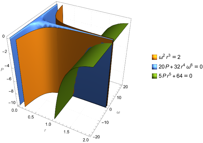
Figure 4: Illustration of the Positivestellensatz and its ability to recover the Radiation Gravitational Wave Power Equation in the special case where $m_{1}=m_{2}=c=G=1$. Keeping other variables constant, the points that obey the power equation are the intersection of the points that obey Kepler’s Third Law and the points of a linearized equation from general relativity, and the wave equation is recoverable by adding these other equations with appropriate polynomial multipliers.

2.9 Bell Inequalities

We now consider the problem of deriving Bell Inequalities in quantum mechanics. Bell Inequalities (bell1964einstein, ) are well-known in physics, because they provide bounds on the correlation of measurements in any multi-particle system which obeys local realism (i.e., for which a joint probability distribution exists), that are violated experimentally, thus demonstrating that the natural world does not obey local realism. For ease of exposition, we prove a version called the GHZ inequality greenberger1990bell . Namely, given random variables $A,B,C$ which take values on $\{\pm 1\}$, for any joint probability distribution describing $A,B,C$, it follows that

$$\mathbb{P}(A=B)+\mathbb{P}(A=C)+\mathbb{P}(B=C)\geq 1,$$ (43)

but this bound is violated experimentally fahmi2002locality .

We derive this result axiomatically, using Kolmogorov’s probability axioms and the specialization of our sum-of-squares framework to linear optimization proposed in Section 2.4, which is a valid specialization because the entire problem is linear. In particular, letting $p_{-1,1,-1}=\mathbb{P}(A=-1,B=1,C=-1)$, deriving the largest lower bound for which this inequality holds is equivalent to solving the following linear optimization problem:

$$\min~{}p_{AB}+p_{BC}+p_{AC}~{}~{}\text{s.t.}~{}~{}p\in\mathcal{S},$$

where $\mathcal{S}:=\{\bm{p}\geq\bm{0},\bm{e}^{\top}\bm{p}=1\}$, $p_{AB}:=p_{-1,-1,-1}+p_{-1,-1,1}+p_{1,1,-1}+p_{1,1,1}$ and $p_{AC}$, $p_{BC}$ are defined similarly.

We solve this problem using Gurobi and Julia, which verifies that $\gamma=1$ is the largest value for which this inequality holds, and obtains the desired inequality. Moreover, the solution to its dual problem yields the certificate $2p_{-1,-1,-1}+2p_{1,1,1}\geq 0$ which verifies that $1$ is indeed a valid lower bound for $p_{AB}+p_{BC}+p_{AC}$, by adding $\bm{e}^{\top}\bm{p}$ to the left-hand side of this certificate and $1$ to the right-hand side.

To further demonstrate the generality and utility of our approach, we now derive a more challenging Bell inequality, namely the so-called I3322 inequality (c.f. froissart1981constructive ). Given particles $A_{1},A_{2},A_{3},B_{1},B_{2},B_{3}$ which take values on $\{\pm 1\}$, the inequality reveals that for any joint probability distribution, we have:

$$\mathbb{E}[A_{1}]-\mathbb{E}[A_{2}]+\mathbb{E}[B_{1}]-\mathbb{E}[B_{2}] -\mathbb{E}[(A_{1}-A_{2})(B_{1}-B_{2})]$$

$$+\mathbb{E}[(A_{1}+A_{2})B_{3}]+\mathbb{E}[A_{3}(B_{1}+B_{2})]\leq 4.$$

Using the same approach as previously, and defining $\bm{p}$ to be an arbitrary discrete probability measure on $\{\pm 1\}^{6}$, we verify that the smallest such upper bound which holds for each joint probability measure is $4$, with the following polynomial certificate modulo $\bm{e}^{\top}\bm{p}=1$:

$$4p_{2,1,1,1,1,1}+4p_{1,2,1,1,1,1}+8p_{2,2,1,1,1,1}+4p_{2,1,2,1,1,1}+4p_{1,2,2,1,1,1}+8p_{2,2,2,1,1,1}$$

$$+4p_{1,1,1,2,1,1}+8p_{2,1,1,2,1,1}+4p_{1,2,1,2,1,1}+8p_{2,2,1,2,1,1}+4p_{2,1,2,2,1,1}+4p_{2,2,2,2,1,1}$$

$$+4p_{1,1,1,1,2,1}+4p_{2,1,1,1,2,1}+12p_{1,2,1,1,2,1}+12p_{2,2,1,1,2,1}+8p_{1,2,2,1,2,1}+8p_{2,2,2,1,2,1}$$

$$+8p_{1,1,1,2,2,1}+8p_{2,1,1,2,2,1}+12p_{1,2,1,2,2,1}+12p_{2,2,1,2,2,1}+4p_{1,2,2,2,2,1}+4p_{2,2,2,2,2,1}$$

$$+4p_{1,1,2,1,1,2}+4p_{2,1,2,1,1,2}+4p_{1,2,2,1,1,2}+4p_{2,2,2,1,1,2}+4p_{1,1,1,2,1,2}+4p_{2,1,1,2,1,2}$$

$$+4p_{1,1,2,2,1,2}+4p_{2,1,2,2,1,2}+4p_{1,1,1,1,2,2}+8p_{1,2,1,1,2,2}+4p_{2,2,1,1,2,2}+4p_{1,1,2,1,2,2}$$

$$+8p_{1,2,2,1,2,2}+4p_{2,2,2,1,2,2}+8p_{1,1,1,2,2,2}+4p_{2,1,1,2,2,2}+8p_{1,2,1,2,2,2}+4p_{2,2,1,2,2,2}$$

$$+4p_{1,1,2,2,2,2}+4p_{1,2,2,2,2,2}\geq 0$$

where an index of $1$ denotes that a random variable took the value $-1$ and an index of $2$ denotes that a random variable took the value $1$, and the random variables are indexed in the order $A_{1},A_{2},A_{3},B_{1},B_{2},B_{3}$.

3 Discussion and Future Developments

In this work, we proposed a new approach to scientific discovery that leverages ideas from real algebraic geometry and mixed-integer optimization to discover new scientific laws from a possibly inconsistent or incomplete set of scientific axioms and noisy experimental data. This notably improves on existing approaches to scientific discovery that typically propose plausible scientific laws from either background theory alone or data alone. Indeed, by combining data and background theory in the discovery process, we potentially allow scientific discoveries to be made in previously inhospitable regimes where there is limited data and/or background theory, and gathering data is expensive. We hope our approach serves as an exciting tool that assists the scientific community in efficiently and accurately explaining the natural world.

Inspired by the success of AI-Hilbert in rediscovering existing scientific laws, we conclude by discussing some exciting research directions that are natural extensions of this work.

Improving the Generality of AI-Hilbert:

This work proposes a symbolic discovery framework that combines background theory expressible as a system of polynomial equalities and inequalities, or that can be reformulated as such a system (e.g., in a Polar coordinate system, by substituting $x=r\cos\theta,y=r\sin\theta$ and requiring that $x^{2}+y^{2}=r^{2}$). However, many scientific discovery contexts involve background theory that cannot easily be expressed via polynomial equalities and inequalities, including differential operators, integrals, and limits, among other operators. Therefore, extending AI-Hilbert to encompass these non-polynomial settings would be of interest.

We point out that several authors have already proposed extensions of the sum-of-squares paradigm beyond polynomial basis functions, and these works offer a promising starting point for performing such an extension. Namely, Löfberg and Parrilo lofberg2004coefficients (see also Bach bach2022sum and Bach and Rudi , bach2023exponential ) propose an extension to trigonometric basis functions, and Fawzi et al. fawzi2019semidefinite propose approximating univariate non-polynomial functions via their Gaussian quadrature and Padé approximants. Moreover, Huchette and Vielma huchette2022nonconvex advocate modeling non-convex functions via piecewise linear approximations with strong dual bounds. Using such polynomial approximations of non-polynomial operators offers one promising path for extending AI-Hilbert to the non-polynomial setting.

Automatically Parameter-Tuning AI-Hilbert:

The version of AI-Hilbert proposed in this paper requires hyperparameter optimization by the user, to trade-off the importance of fidelity to a model, fidelity to experimental data, and complexity of the symbolic model discovered. Therefore, one extension of this work could be to automate this hyperparameter optimization process, by automatically solving mixed-integer and semidefinite optimization problems with different bounds on the degree of the proof certificates and different weights on the relative importance of fidelity to a model and fidelity to data, and using machine learning techniques to select solutions most likely to satisfy a scientist using AI-Hilbert.

Improving the Scalability of AI-Hilbert:

One limitation of our implementation of AI-Hilbert is that it relies on reformulating sum-of-squares optimization problems as semidefinite problems and solving them via primal-dual interior point methods (IPMs) nesterov1994interior ; nesterov1997self . This arguably presents a limitation, because the Newton step in IPMs (see, e.g., alizadeh1998primal, ) requires performing a memory-intensive matrix inversion operation. Indeed, this matrix inversion operation is sufficiently expensive that, in our experience, AI-Hilbert was unable to perform scientific discovery tasks with more than $n=15$ variables and a constraint on the degree of the certificates searched over of $d=20$ or greater (in general, runtime and memory usage is a function of both the number of symbolic variables and the degree of the proof certificates searched over).

To address this limitation and enhance the scalability of AI-Hilbert, there are at least three future directions to explore. First, one could exploit ideas related to the Newton polytope (or convex hull of the exponent vectors of a polynomial) reznick1978extremal to reduce the number of monomials in the sum-of-squares decompositions developed in this paper, as discussed in detail in (blekherman2012semidefinite, , Chap 3.3.4). Second, one could use presolving techniques such as chordal sparsity griewank1984existence ; vandenberghe2015chordal or partial facial reduction permenter2018partial ; zhu2019sieve to reduce the number of variables in the semidefinite optimization problems that arise from sum-of-squares optimization problems. Third, one could attempt to solve sum-of-squares problems without using computationally expensive interior point methods for semidefinite programs, e.g., by using a Burer-Monteiro factorization approach burer2003nonlinear ; legat2022low or by optimizing over a second-order cone inner approximation of the positive semidefinite cone ahmadi2019dsos .

Acknowledgements

We are grateful to Phokion Kolatis, Jon Lenchner, and Ken Clarkson (IBM) for valuable discussions on scientific discovery.

References

- [1] A. A. Ahmadi, E. De Klerk, and G. Hall. Polynomial norms. SIAM Journal on Optimization, 29(1):399–422, 2019.
- [2] A. A. Ahmadi and B. E. Khadir. Learning dynamical systems with side information. SIAM Review, 65(1):183–223, 2023.
- [3] A. A. Ahmadi and A. Majumdar. DSOS and SDSOS optimization: More tractable alternatives to sum of squares and semidefinite optimization. SIAM Journal on Applied Algebra and Geometry, 3(2):193–230, 2019.
- [4] F. Alizadeh, J.-P. A. Haeberly, and M. L. Overton. Primal-dual interior-point methods for semidefinite programming: Convergence rates, stability and numerical results. SIAM Journal on Optimization, 8(3):746–768, 1998.
- [5] E. D. Andersen and K. D. Andersen. The MOSEK interior point optimizer for linear programming: an implementation of the homogeneous algorithm. High Performance Optimization, pages 197–232, 2000.
- [6] A. Arora, S. Belenzon, and A. Patacconi. The decline of science in corporate R&D. Strategic Management Journal, 39(1):3–32, 2018.
- [7] G. B. Arous, A. S. Wein, and I. Zadik. Free energy wells and overlap gap property in sparse pca. In Conference on Learning Theory, pages 479–482. PMLR, 2020.
- [8] E. Artin. Über die zerlegung definiter funktionen in quadrate. In Abhandlungen aus dem mathematischen Seminar der Universität Hamburg, volume 5, pages 100–115. Springer, 1927.
- [9] V. Austel, S. Dash, O. Gunluk, L. Horesh, L. Liberti, G. Nannicini, and B. Schieber. Globally optimal symbolic regression. arXiv preprint arXiv:1710.10720, 2017.
- [10] F. Bach. Sum-of-squares relaxations for information theory and variational inference. arXiv preprint arXiv:2206.13285, 2022.
- [11] F. Bach and A. Rudi. Exponential convergence of sum-of-squares hierarchies for trigonometric polynomials. SIAM Journal on Optimization, 33(3):2137–2159, 2023.
- [12] Z. J. Baum, X. Yu, P. Y. Ayala, Y. Zhao, S. P. Watkins, and Q. Zhou. Artificial intelligence in chemistry: current trends and future directions. Journal of Chemical Information and Modeling, 61(7):3197–3212, 2021.
- [13] J. S. Bell. On the Einstein Podolsky Rosen paradox. Physics Physique Fizika, 1(3):195, 1964.
- [14] D. Bertsimas, R. Cory-Wright, S. Lo, and J. Pauphilet. Optimal low-rank matrix completion: Semidefinite relaxations and eigenvector disjunctions. arXiv preprint arXiv:2305.12292, 2023.
- [15] D. Bertsimas, R. Cory-Wright, and J. Pauphilet. Mixed-projection conic optimization: A new paradigm for modeling rank constraints. Operations Research, 70(6):3321–3344, 2022.
- [16] D. Bertsimas and J. Dunn. Machine learning under a modern optimization lens. Dynamic Ideas Press, 2019.
- [17] D. Bertsimas and W. Gurnee. Learning sparse nonlinear dynamics via mixed-integer optimization. Nonlinear Dynamics, pages 1–20, 2023.
- [18] D. Bertsimas, A. King, and R. Mazumder. Best subset selection via a modern optimization lens. The Annals of Statistics, 44(2):813 – 852, 2016.
- [19] J. Bhattacharya and M. Packalen. Stagnation and scientific incentives. Technical report, National Bureau of Economic Research, 2020.
- [20] R. Bixby and E. Rothberg. Progress in computational mixed integer programming–a look back from the other side of the tipping point. Annals of Operations Research, 149(1):37, 2007.
- [21] G. Blekherman, P. A. Parrilo, and R. R. Thomas. Semidefinite optimization and convex algebraic geometry. SIAM, 2012.
- [22] J. Bongard and H. Lipson. Automated reverse engineering of nonlinear dynamical systems. Proceedings of the National Academy of Sciences, 104(24):9943–9948, 2007.
- [23] S. L. Brunton, J. L. Proctor, and J. N. Kutz. Discovering governing equations from data by sparse identification of nonlinear dynamical systems. Proceedings of the National Academy of Sciences, 113(15):3932–3937, 2016.
- [24] E. Brynjolfsson, D. Rock, and C. Syverson. Artificial intelligence and the modern productivity paradox: A clash of expectations and statistics. In The economics of artificial intelligence: An agenda, pages 23–57. University of Chicago Press, 2018.
- [25] S. Burer and R. D. Monteiro. A nonlinear programming algorithm for solving semidefinite programs via low-rank factorization. Mathematical Programming, 95(2):329–357, 2003.
- [26] E. J. Candes and Y. Plan. Matrix completion with noise. Proceedings of the IEEE, 98(6):925–936, 2010.
- [27] C.-W. Chou, D. B. Hume, T. Rosenband, and D. J. Wineland. Optical clocks and relativity. Science, 329(5999):1630–1633, 2010.
- [28] M. Clegg, J. Edmonds, and R. Impagliazzo. Using the Gröebner basis algorithm to find proofs of unsatisfiability. In Proceedings of the twenty-eighth annual ACM symposium on Theory of computing, pages 174–183, 1996.
- [29] C. Cornelio, S. Dash, V. Austel, T. Josephson, J. Goncalves, K. Clarkson, N. Megiddo, B. E. Khadir, and L. Horesh. Combining data and theory for derivable scientific discovery with AI-Descartes. Nature Communications, 14(1777), 2023.
- [30] T. Cowen. The great stagnation: How America ate all the low-hanging fruit of modern history, got sick, and will (eventually) feel better: A Penguin eSpecial from Dutton. Penguin, 2011.
- [31] D. Cox, J. Little, and D. O’Shea. Ideals, varieties, and algorithms: An introduction to computational algebraic geometry and commutative algebra. Springer Science & Business Media, 2013.
- [32] A. Cozad and N. V. Sahinidis. A global MINLP approach to symbolic regression. Mathematical Programming, 170:97–119, 2018.
- [33] M. Cranmer. PySR: Fast and parallelized symbolic regression in Python/Julia. 4052869, 2020.
- [34] M. Curmei and G. Hall. Shape-constrained regression using sum of squares polynomials. Operations Research, 2023.
- [35] H. W. De Regt. Understanding, values, and the aims of science. Philosophy of Science, 87(5):921–932, 2020.
- [36] S. S. Dey, Y. Dubey, and M. Molinaro. Branch-and-bound solves random binary ips in polytime. In Proceedings of the 2021 ACM-SIAM Symposium on Discrete Algorithms (SODA), pages 579–591. SIAM, 2021.
- [37] P. A. Dirac. Directions in physics. Lectures delivered during a visit to Australia and New Zealand, August/September 1975. 1978.
- [38] R. Dubčáková. Eureqa: software review, 2011.
- [39] M. R. Engle and N. V. Sahinidis. Deterministic symbolic regression with derivative information: General methodology and application to equations of state. AIChE Journal, 68(6):e17457, 2022.
- [40] A. Fahmi. Locality, Bell’s inequality and the GHZ theorem. Physics Letters A, 303(1):1–6, 2002.
- [41] A. Fawzi, M. Malinowski, H. Fawzi, and O. Fawzi. Learning dynamic polynomial proofs. Advances in Neural Information Processing Systems, 32, 2019.
- [42] H. Fawzi, J. Saunderson, and P. A. Parrilo. Semidefinite approximations of the matrix logarithm. Foundations of Computational Mathematics, 19:259–296, 2019.
- [43] R. P. Feynman, R. B. Leighton, and M. Sands. The Feynman lectures on physics; vol. i. American Journal of Physics, 33(9):750–752, 1965.
- [44] M. Froissart. Constructive generalization of Bell’s inequalities. Nuovo Cimento B;(Italy), 64(2), 1981.
- [45] N. Fujinuma, B. DeCost, J. Hattrick-Simpers, and S. E. Lofland. Why big data and compute are not necessarily the path to big materials science. Communications Materials, 3(1):59, 2022.
- [46] N. Fulton, S. Mitsch, J.-D. Quesel, M. Völp, and A. Platzer. KeYmaera X: An axiomatic tactical theorem prover for hybrid systems. In Automated Deduction-CADE-25: 25th International Conference on Automated Deduction, Berlin, Germany, August 1-7, 2015, Proceedings 25, pages 527–538. Springer, 2015.
- [47] D. Gamarnik and I. Zadik. High dimensional regression with binary coefficients. estimating squared error and a phase transtition. In Conference on Learning Theory, pages 948–953. PMLR, 2017.
- [48] D. M. Greenberger, M. A. Horne, A. Shimony, and A. Zeilinger. Bell’s theorem without inequalities. American Journal of Physics, 58(12):1131–1143, 1990.
- [49] A. Griewank and P. L. Toint. On the existence of convex decompositions of partially separable functions. Mathematical Programming, 28:25–49, 1984.
- [50] R. Guimerà, I. Reichardt, A. Aguilar-Mogas, F. A. Massucci, M. Miranda, J. Pallarès, and M. Sales-Pardo. A Bayesian machine scientist to aid in the solution of challenging scientific problems. Science Advances, 6(5):eaav6971, 2020.
- [51] S. D. Gupta, B. P. Van Parys, and E. K. Ryu. Branch-and-bound performance estimation programming: A unified methodology for constructing optimal optimization methods. Mathematical Programming, 2023.
- [52] G. Hall. Applications of sums of squares polynomials. In P. Parrilo and R. Thomas, editors, Sum of Squares: Theory and Applications, volume 77. Proceedings of Symposia in Applied Mathematics, 2020.
- [53] D. Hilbert. Über die darstellung definiter formen als summe von formenquadraten. Mathematische Annalen, 32(3):342–350, 1888.
- [54] J. Huchette and J. P. Vielma. Nonconvex piecewise linear functions: Advanced formulations and simple modeling tools. Operations Research, 2022.
- [55] R. A. Hulse and J. H. Taylor. Discovery of a pulsar in a binary system. The Astrophysical Journal, 195:L51–L53, 1975.
- [56] R. Iten, T. Metger, H. Wilming, L. Del Rio, and R. Renner. Discovering physical concepts with neural networks. Physical Review Letters, 124(1):010508, 2020.
- [57] I. M. Johnstone and A. Y. Lu. On consistency and sparsity for principal components analysis in high dimensions. Journal of the American Statistical Association, 104(486):682–693, 2009.
- [58] G. Karagiorgi, G. Kasieczka, S. Kravitz, B. Nachman, and D. Shih. Machine learning in the search for new fundamental physics. Nature Reviews Physics, 4(6):399–412, 2022.
- [59] H. Kitano. Nobel turing challenge: creating the engine for scientific discovery. npj Systems Biology and Applications, 7(1):29, 2021.
- [60] J.-L. Krivine. Anneaux préordonnés. Journal d’analyse mathématique, 12:p–307, 1964.
- [61] J. Kubalík, E. Derner, and R. Babuška. Symbolic regression driven by training data and prior knowledge. In Proceedings of the 2020 Genetic and Evolutionary Computation Conference, pages 958–966, 2020.
- [62] J. Kubalík, E. Derner, and R. Babuška. Multi-objective symbolic regression for physics-aware dynamic modeling. Expert Systems with Applications, 182:115210, 2021.
- [63] M. Landajuela, C. S. Lee, J. Yang, R. Glatt, C. P. Santiago, I. Aravena, T. Mundhenk, G. Mulcahy, and B. K. Petersen. A unified framework for deep symbolic regression. Advances in Neural Information Processing Systems, 35:33985–33998, 2022.
- [64] J. B. Lasserre. Global optimization with polynomials and the problem of moments. SIAM Journal on Optimization, 11(3):796–817, 2001.
- [65] J. B. Lasserre. A sum of squares approximation of nonnegative polynomials. SIAM Review, 49(4):651–669, 2007.
- [66] M. Laurent. Sums of squares, moment matrices and optimization over polynomials. In Emerging Applications of Algebraic Geometry, pages 157–270. Springer, 2009.
- [67] M. Laurent and F. Rendl. Semidefinite programming and integer programming. Handbooks in Operations Research and Management Science, 12:393–514, 2005.
- [68] B. Legat, C. Yuan, and P. A. Parrilo. Low-rank univariate sum of squares has no spurious local minima. arXiv preprint arXiv:2205.11466, 2022.
- [69] J. Lofberg and P. A. Parrilo. From coefficients to samples: A new approach to SOS optimization. In 2004 43rd IEEE Conference on Decision and Control (CDC)(IEEE Cat. No. 04CH37601), volume 3, pages 3154–3159. IEEE, 2004.
- [70] Y. Matsubara, N. Chiba, R. Igarashi, and Y. Ushiku. SRSD: Rethinking datasets of symbolic regression for scientific discovery. In NeurIPS 2022 AI for Science: Progress and Promises, 2022.
- [71] Y. Nesterov and A. Nemirovskii. Interior-point polynomial algorithms in convex programming. SIAM, 1994.
- [72] Y. E. Nesterov and M. J. Todd. Self-scaled barriers and interior-point methods for convex programming. Mathematics of Operations Research, 22(1):1–42, 1997.
- [73] OpenAI. GPT-4 technical report. arXiv preprint arXiv:2303.08774, 2023.
- [74] P. A. Parrilo. Semidefinite programming relaxations for semialgebraic problems. Mathematical Programming, 96(2):293–320, 2003.
- [75] F. Permenter and P. Parrilo. Partial facial reduction: Simplified, equivalent SDPs via approximations of the PSD cone. Mathematical Programming, 171:1–54, 2018.
- [76] P. C. Peters and J. Mathews. Gravitational radiation from point masses in a Keplerian orbit. Physical Review, 131(1):435, 1963.
- [77] M. Putinar. Positive polynomials on compact semi-algebraic sets. Indiana University Mathematics Journal, 42(3):969–984, 1993.
- [78] M. V. Ramana. An exact duality theory for semidefinite programming and its complexity implications. Mathematical Programming, 77:129–162, 1997.
- [79] A. Reuther, J. Kepner, C. Byun, S. Samsi, W. Arcand, D. Bestor, B. Bergeron, V. Gadepally, M. Houle, M. Hubbell, M. Jones, A. Klein, L. Milechin, J. Mullen, A. Prout, A. Rosa, C. Yee, and P. Michaleas. Interactive supercomputing on 40,000 cores for machine learning and data analysis. In 2018 IEEE High Performance extreme Computing Conference (HPEC), pages 1–6. IEEE, 2018.
- [80] B. Reznick. Extremal PSD forms with few terms. Duke Mathematical Journal, 45(2):363–374, 1978.
- [81] C. Rudin. Stop explaining black box machine learning models for high stakes decisions and use interpretable models instead. Nature Machine Intelligence, 1(5):206–215, 2019.
- [82] S. H. Rudy, S. L. Brunton, J. L. Proctor, and J. N. Kutz. Data-driven discovery of partial differential equations. Science Advances, 3(4):e1602614, 2017.
- [83] J. L. Russell. Kepler’s laws of planetary motion: 1609–1666. The British Journal for the History of Science, 2(1):1–24, 1964.
- [84] M. Schmidt and H. Lipson. Distilling free-form natural laws from experimental data. Science, 324(5923):81–85, 2009.
- [85] M. Schmidt and H. Lipson. Symbolic regression of implicit equations. In Genetic Programming Theory and Practice VII, pages 73–85. Springer, 2009.
- [86] K. Schmüdgen. The moment problem on compact semi-algebraic sets. Mathematische Annalen, 289:283–313, 1991.
- [87] H. A. Simon. Does scientific discovery have a logic? Philosophy of Science, 40(4):471–480, 1973.
- [88] G. Stengle. A Nullstellensatz and a Positivstellensatz in semialgebraic geometry. Mathematische Annalen, 207(2):87–97, 1974.
- [89] S.-M. Udrescu, A. Tan, J. Feng, O. Neto, T. Wu, and M. Tegmark. AI Feynman 2.0: Pareto-optimal symbolic regression exploiting graph modularity. Advances in Neural Information Processing Systems, 33:4860–4871, 2020.
- [90] S.-M. Udrescu and M. Tegmark. AI Feynman: A physics-inspired method for symbolic regression. Science Advances, 6(16), 2020.
- [91] L. Vandenberghe, M. S. Andersen, et al. Chordal graphs and semidefinite optimization. Foundations and Trends® in Optimization, 1(4):241–433, 2015.
- [92] H. Wang, T. Fu, Y. Du, W. Gao, K. Huang, Z. Liu, P. Chandak, S. Liu, P. Van Katwyk, A. Deac, et al. Scientific discovery in the age of artificial intelligence. Nature, 620(7972):47–60, 2023.
- [93] W. Wang, M. J. Wainwright, and K. Ramchandran. Information-theoretic limits on sparse signal recovery: Dense versus sparse measurement matrices. IEEE Transactions on Information Theory, 56(6):2967–2979, 2010.
- [94] H. Weyl. Quantenmechanik und gruppentheorie. Zeitschrift für Physik, 46(1):1–46, 1927.
- [95] W. Zhao and G. Zhou. Hausdorff distance between convex semialgebraic sets. Journal of Global Optimization, pages 1–21, 2023.
- [96] Y. Zhu, G. Pataki, and Q. Tran-Dinh. Sieve-SDP: A simple facial reduction algorithm to preprocess semidefinite programs. Mathematical Programming Computation, 11:503–586, 2019.