INR-LDDMM: Fluid-based Medical Image Registration Integrating Implicit Neural Representation and Large Deformation Diffeomorphic Metric Mapping

Abstract

We propose a fluid-based registration framework of medical images based on implicit neural representation. By integrating implicit neural representation and Large Deformable Diffeomorphic Metric Mapping (LDDMM), we employ a Multilayer Perceptron (MLP) as a velocity generator while optimizing velocity and image similarity. Moreover, we adopt a coarse-to-fine approach to address the challenge of deformable-based registration methods dropping into local optimal solutions, thus aiding the management of significant deformations in medical image registration. Our algorithm has been validated on a paired CT-CBCT dataset of 50 patients,taking the Dice coefficient of transferred annotations as an evaluation metric. Compared to existing methods, our approach achieves the state-of-the-art performance.

Index Terms—  Implicit Neural Representation(INR), Medical Image Registration, LDDMM

1 Introduction

Medical image registration is a critical part of medical image processing, aiding in the collection and integration of information from various image sources. The registration process involves modifying the geometric configuration of one image to align with another, thereby establishing a mapping relationship between the respective points. This is indispensable for many medical image processing applications, such as in Image Guided Radiation Therapy (IGRT).

The techniques for volumetric image registration can be mainly categorized into two: traditional iterative-based methods and deep learning methods. Traditional iterative-based methods such as bUnwarpJ [1], NiftyReg [2], RVSS [1], ANTs [3], DROP [4], and Elastix [5], hold the advantage of optimizing each image individually; however, typically they are slower, susceptible to getting stuck in local optima, with complicated parameter optimization. Traditional iterative methods can further be split into displacement field optimized registration methods and velocity field optimized registration methods.

Displacement field optimized methods, often referred to as elastic registrations, include techniques like Demos. Velocity field optimized methods, commonly known as Fluid registration methods, often possess superior diffeomorphism and physical properties (for example, better intermediate state images can be obtained). Examples of Fluid registration methods include vSVF and LDDMM[6]. vSVF makes the assumption that velocity doesn’t transform with time, aiming to search for the initial momentum. LDDMM considers the speed $v(x,t)$ as a function of position and time, optimizing for image similarity and speed, with the intent to seek the best initial momentum.

Deep learning-based methods rose to prominence with voxelmorph[7], which is an unsupervised learning-based approach for deformable medical image registration. It uses a Convolutional Neural Network (CNN) to approximate the registration function by minimizing image dissimilarity and a regularization term that encourages smooth spatial transformations. However, the performance of deep learning-based methods highly depends on the dataset, and performs poorly when the dataset is scarce or there is a large variance between training and test datasets.

Implicit Neural Representation is an emerging technology[8, 9, 10]. It uses neural networks to implicitly represent complex functions, shapes and structures in high-dimensional spaces. This representation can generate highly detailed outputs while having parameters with relatively small dimensions. Recently, [11] proposed the registration method based on the implicit neural representation of displacement field estimation. It uses Multi Layer Perceptron (MLP) to establish the mapping relationship between position and deformation, optimizing it with similarity and regulation. [12] introduced a Velocity field estimation-based registration method of implicit neural representation.But the velocity field in the [12] is not changing over time.

The IGRT is an essential technology for precise radiation transfer. In the domain of IGRT, CBCT is frequently used due to its rapid acquisition[13, 14, 15], cost effectiveness and low radiation dose advantages. However, CBCT images usually exhibit a lower contrast for soft tissues, limited anatomical details, and increased artifacts due to reduced radiation and insufficient projection data. In contrast, CT images provide superior voxel value, noise reduction and spatial uniformity, making them more suitable for treatment planning.Therefore we need to align the planned CT to the CBCT to provide more detail and structure to the physician.

The contributions of this paper are as follows:

(i) Proposed the first time-space correlated velocity field estimation implicit neural representation by integrating Implicit Neural Representation with LDDMM.

(ii) Optimized the speed of INR-LDDMM with a coarse-to-fine framework.

(iii) Validated on a paired CT-CBCT interstitial lung disease dataset from 50 patient prognoses, achieving state-of-the-art results.

2 Method

In the proposed approach, we incorporate a Multilayer Perceptron (MLP) consisting of three layers into the Large Deformation Diffeomorphic Metric Mapping (LDDMM) framework. Initially, we formalize our problem (Section 2.1), followed by the presentation of the INR-LDDMM framework (Section 2.2). Finally, based on INR-LDDMM, we introduce improvements using a Coarse-to-Fine method (Section 2.3).

2.1 Problem Formulation

In the field of medical image registration, the Large Deformation Diffeomorphic Metric Mapping (LDDMM) is a fluid-based image registration model[16], that calculates the spatial transformation $\varphi$ by computing a spatio-temporal velocity field $v(t,x)$. This is achieved through integration $\partial_{t}\varphi(t,x)=v(t,\varphi(t,x)),\leavevmode\nobreak\ \varphi(0,x)=x$. For an appropriately regularized velocity field, it guarantees the diffeomorphic form transformation[17]. In medical imaging tasks, we need to align the moving image to a fixed image. We denote the moving image of size $a\times b\times c$ as $I_{1}$, and $I_{2}$ represents the fixed image of the same size. The underlying LDDMM optimization problem can be written as:

$$\mathcal{L}=\underset{v}{\text{argmin}}\leavevmode\nobreak\ {Sim}(I_{1}(1),I_{2})+\frac{1}{2}\int_{0}^{1}\|v(t)\|^{2}_{L}dt,$$ (1)

satisfying $\partial_{t}I+\langle\nabla I,v\rangle=0,\leavevmode\nobreak\ I_{1}(0)=I_{1}$, where $I_{1}(t)$ represents the moving image over time, with $I_{1}(1)$ being the final moved image. $\nabla$ signifies the gradient, $\langle\cdot,\cdot\rangle$ denotes the inner product and $Sim(A,B)$ signifies the similarity measurement between images. We assume the displacement field from $I_{1}$ to $I1(t)$ is $S$. Thereby, the optimization problem is mathematically presented as:

$$\underset{v}{\arg\min}\ \mathrm{Sim}(I_{1}\circ S,I_{2})+\frac{1}{2}\int_{0}^{1}\|v(t)\|^{2}_{L}dt,$$ (2)

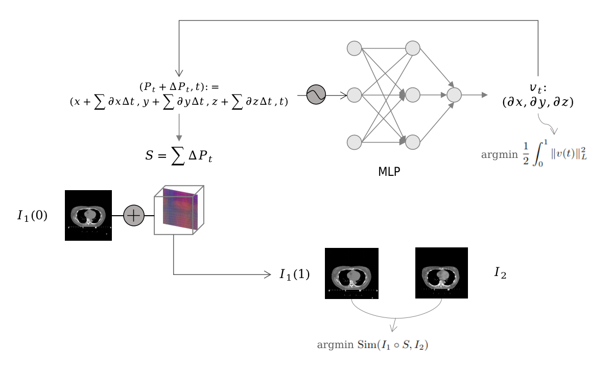
Fig. 1: Illustration of INR-LDDMM. We input the time t and the position coordinates corresponding to moment t into the MLP network to obtain the velocity at the corresponding moment. Based on the velocity we can get the amount of change in position and thus input the position and time of the next moment to predict the velocity of the next moment. According to the LDDMM model, our optimization objectives are the velocity and the similarity between the moved image and the fixed image.

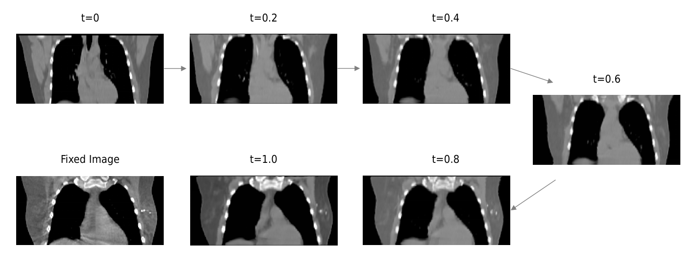
Fig. 2: The figure represents the transformation of the moving image over time. It can be seen that the moving image gradually and ’naturally’ turns into a moved image over time.

Type	Method	CTV	Heart	Left Lung	Right Lung	Spinal	Aorta	Scapula	Average
Learning-based	TransMorph	0.83	0.82	0.90	0.89	0.67	0.76	0.73	0.80
	VoxelMorph	0.79	0.78	0.89	0.90	0.62	0.73	0.73	0.77
Iteration-based	Demos	0.89	0.88	0.93	0.93	0.69	0.80	0.79	0.84
	Elastix	0.91	0.92	0.94	0.95	0.77	0.86	0.80	0.88
INR-based	INR only	0.90	0.92	0.95	0.95	0.77	0.87	0.81	0.87
	Ours	0.92	0.95	0.97	0.97	0.79	0.88	0.84	0.91

Table 1: Comparison of results with other methods. The methods are classified as Learning-based, Iteration-based and INR-based. The values in the table are DSC values.

where $\mathrm{Sim}(I_{1}\circ S,I_{2})$ represents the similarity measure between the transformed moving image and the fixed image.

2.2 INR-LDDMM

The INR-LDDMM framework is schematically shown in Fig.1. We initially commence with a three-layered Multilayer Perceptron (MLP) network. The design and development of this MLP network aims to replace conventional velocity field estimation within the Large Deformation Diffeomorphic Metric Mapping (LDDMM). Specifically, it assists us in predicting local velocities at any given position within 3D images. We define $\mathcal{X}=(x,y,z,t)$ as spatial positions and time variables continuously inputted to MLP. The corresponding time velocity is the output of the network, denoted as $\mathcal{V}=(v_{x},v_{y},v_{z})$. It is recognized that the relationship between displacement in space $(\Delta x,\Delta y,\Delta z)$ and velocity $\mathcal{V}=(v_{x},v_{y},v_{z})=(\partial x,\partial y,\partial z)$ is represented as:

$$(\Delta x,\Delta y,\Delta z)=(\int v_{x}dt,\int v_{y}dt,\int v_{z}dt)$$

This equation has a discrete representation, thus the input $\mathcal{X}=(x+\Delta x,y+\Delta y,z+\Delta z,t)$ can be denoted as

$$(P_{t}+\Delta P_{t},t)=(x+\partial x\Delta t,y+\partial y\Delta t,z+\partial z\Delta t,t)$$ (3)

Consequently, for a given time interval $\Delta t$, after obtaining the corresponding velocities $(\partial x,\partial y,\partial z)$ through our velocity estimation MLP, we next determine the new input $\mathcal{X}=(x+\partial x\Delta t,y+\partial y\Delta t,z+\partial z\Delta t,t)$. If we use $f(\mathcal{X})$ to represent MLP, this process is formulated as:

$$\mathcal{V}=f(\mathcal{X})$$ (4)

$$\mathcal{X}=(P_{t}+\Delta P_{t},t)$$ (5)

$$\Delta P_{t}=\mathcal{V}*\delta t=f(\mathcal{X})*\delta t$$ (6)

We can then obtain the displacement field:

$$S=\Sigma\Delta P_{t}=\Sigma[(\partial x\Delta t,\partial y\Delta t,\partial z\Delta t)]$$

Based on the preceding optimization goal, our current loss function to optimize is:

$$L= \underset{S}{\mathrm{argmin}}(Sim(I_{1}\circ S,I_{2})+\frac{1}{n}\sum_{i=1}^{n}\|v_{i}\|^{2}_{L})$$ (7)

$$= \underset{S}{\mathrm{argmin}}(Sim(I_{1}\circ\sum_{t=1}^{n}f(\mathcal{X}_{t})*\delta t,I_{2})$$ (8)

$$+\frac{1}{n}\sum_{t=1}^{n}\|f(\mathcal{X}_{t})*\delta t\|^{2}_{L})$$ (9)

Here, $\mathcal{X}_{t}$ represents the input at each step, encompassing position and time, and $f(\mathcal{X}_{t})$ indicates the output from the MLP network at the corresponding time, that is, the velocity. The $\circ$ and $\sum$ operators within the $Sim$ term designate the warping operation and the accumulation across all time-steps respectively.

We then utilize gradient descent to update the parameters of the MLP network by solving the gradient of the loss function $L$. Iterating over this procedure continuously until satisfaction of a stopping criterion (e.g., achieving a predetermined number of iterations or loss reduction to a certain threshold), we finally return the resultant displacement field $S$, which plays a vital role in transforming from the moving image $I_{1}$ to the stationary image $I_{2}$.

2.3 Coarse-to-fine Framework

The direct optimization of high-resolution velocity fields could escalate the complexity of MLP optimization in proportion to the resolution. This tendency might trap the network in local optima more easily, besides prolonging the training duration. Consequently, we integrate a coarse-to-fine training mechanism into the INR-LDDMM framework.

We initiate the optimization at a coarse stage. The velocity field resolution at this stage, denoted as $(m_{x},m_{y},m_{z})$, enables us to generate a rough displacement field, $S_{1}$, through the INR-LDDMM algorithm,

$$S_{1}=\text{INR-LDDMM}((m_{x},m_{y},m_{z}),(I_{1},I_{2}),n,MLP_{\text{param0}})$$ (10)

where $MLP_{\text{param0}}$ represents the initially set MLP parameters, and $n$ denotes the iterations number. We define the resolution of the fine-stage velocity field as $(M_{x},M_{y},M_{z})$. First, we need to interpolate $S_{1}$ from the low resolution $(m_{x},m_{y},m_{z})$ to a high resolution $(M_{x},M_{y},M_{z})$ via bilinear interpolation. We denote the interpolation results as $S_{1}’$ and utilize them for MLP network parameter optimization. The optimization objective is given by

$$L={\mathrm{argmin}}\left\{\|S-S_{1}^{\prime}\|^{2}_{L}+\frac{1}{n}\sum_{i=1}^{n}\|v_{i}\|^{2}_{L}\right\}$$ (11)

where $S=\Sigma[(\partial x\Delta t,\partial y\Delta t,\partial z\Delta t)]$. Subsequently, we transfer the optimized MLP parameters, $MLP{\text{param}}$, into the fine-stage INR-LDDMM. It is given by:

$$S_{f}=\text{INR-LDDMM}(M_{x},M_{y},M_{z},(I_{1},I_{2}),n,MLP_{\text{param}})$$ (12)

The final displacement field we aim for is $S_{f}$. The moved image $I_{1}(1)$ that we ultimately wish to obtain is:

$$I_{1}(1)=I_{1}(0)\circ S_{f}$$ (13)

3 Results

3.1 Dataset

In this analysis, we studied a cohort of 50 patients who had received radiotherapy post-breast-conserving surgery. The study design involved paired CT-CBCT data. For each patient, we adhered to the standard treatment planning procedure, necessitating the procurement of CT images and at least one set of CBCT images throughout their treatment course.Initial cropping was done for CT and CBCT to ensure that they were in the same range. Both CT-CBCT images were 256*256*96 in size. Both CT and CBCT were labeled with segmentation masks, including CTV , Heart , Left Lung , Right Lung, Aorta, Scapula and Spinal Cord.

3.2 Experiments

We compare with deep learning based methods and traditional methods, and find that INR-LDDMM substantially leads other algorithms. The learning-based methods’ results are averaged over five-fold cross-validation. The quantitative results are shown in Table 1. As shown in the figure, we show the results of the velocity field acting on the moving image for different time periods. It can be seen that the moving image is ’naturally’ turned into a moved image at different time points.

Algorithm 1 INR-LDDMM for Medical Image Registration

1:  Intialize three-layer MLP network

2:  Define $I_{1}$ as moving image and $I_{2}$ as fixed image.

3:  Define $n$ as the time-step interval

4:  Define $N_{x}$,$N_{y}$,$N_{z}$ as the density of the displacement field in the x, y, and z directions.

5:  for each position $p=(x,y,z)$ in $Meshgrid(0:1:N_{x},0:1:N_{y},0:1:N_{z})$, and time $t$ do

6:     Predict velocity $v_{p}=(\delta x,\delta y,\delta z)$ using MLP network

7:     Update position $p$ as $p+v_{p}\delta t$

8:     Update time $t$ as $t-\delta t$

9:     if time step divisible by $n$ then

10:        Save velocity $v_{p}$ as $v_{i|p}$, where $i=\lfloor t/n\rfloor$

11:     end if

12:  end for

13:  Save velocity $v_{i|p}$ in every $p$ as velocity field $v_{i}$.

14:  Compute displacement field $S$ as average of $v_{1}t,v_{2}t,\ldots,v_{n}t$

15:  Compute loss as:

$$L=\underset{S}{\mathrm{argmin}}\left\{Sim(I_{1}\circ S,I_{2})+\frac{1}{n}\sum_{i=1}^{n}\|v_{i}\|^{2}_{L}\right\}$$

16:  Optimize MLP network using gradient descent or another optimizer to minimize $L$

17:  if stopping criterion fulfilled then

18:     Exit loop

19:  else

20:     Return to step 5

21:  end if

22:  return  displacement field $S$

Algorithm 2 Coarse-to-Fine INR-LDDMM for Medical Image Registration

1:  Initialize three-layer MLP network

2:  Set moving image $I_{1}$, fixed image $I_{2}$, time-step interval $n$, density of fine displacement field $(M_{x},M_{y},M_{z})$ and density of coarse displacement field $(m_{x},m_{y},m_{z})$.

3:  Define INR-LDDMM(($N_{x}$,$N_{y}$,$N_{z}$),($I_{1}$,$I_{2}$),n,$MLP_{param}$) as Algorithm 1.($N_{x}$,$N_{y}$,$N_{z}$) is density of the displacement field, ($I_{1}$,$I_{2}$) is image pair of fixed image and moving image,n is the time-step interval and $MLP_{param}$ is incoming parameters of MLP.

4:  $S_{1}$ = INR-LDDMM(($m_{x}$,$m_{y}$,$m_{z}$),($I_{1}$,$I_{2}$),n,$MLP_{param0}$)

5:  Interpolate $S_{1}$ to the density of $(M_{x},M_{y},M_{z})$, denoted as $S_{1}^{\prime}$.

6:  for each $p=(x,y,z)$ and $t$ do

7:     Predict velocity $v_{i|p}=(\delta x,\delta y,\delta z)$ using MLP network

8:     $p\leftarrow p+v_{i|p}\delta t$

9:     $t\leftarrow t-\delta t$

10:     if time step divisible by $n$ then

11:        Save velocity $v_{i|p}$, where $i=\lfloor t/n\rfloor$

12:     end if

13:  end for

14:  Save velocity $v_{i|p}$ in every $p$ as velocity field $v_{i}$.

15:  Compute displacement field $S$ as average of $v_{1}t,v_{2}t,\ldots,v_{n}t$

16:  Compute loss as:

$$L={\mathrm{argmin}}\left\{\|S-S_{1}^{\prime}\|^{2}_{L}+\frac{1}{n}\sum_{i=1}^{n}\|v_{i}\|^{2}_{L}\right\}$$

17:  Optimize MLP network using gradient descent or another optimizer to minimize $L$

18:  if stopping criterion fulfilled then

19:     Exit loop

20:  else

21:     Return to step 6

22:  end if

23:  return  $MLP_{Param}$.

24:  $S_{f}$ = INR-LDDMM($M_{x}$,$M_{y}$,$M_{z}$,($I_{1}$,$I_{2}$),n , $MLP_{param}$).

25:  return  displacement field $S_{f}$

4 Conclusion

In this study, we proposed a novel registration algorithm named INR-LDDMM that integrates the effectiveness of Implicit Neural Representation into the Large Deformable Diffeomorphic Metric Mapping method.With extensive experiments on datasets consisting of paired CT-CBCT images, INR-LDDMM consistently outperformed traditional and deep learning-based medical image registration methods.

5 Compliance with Ethical Standards

This retrospective study was approved by the ethics committee of Ethics Committee of Sun Yat-sen University Cancer Center (SL-G2023-052-01).

6 Acknowledgments

This work is partly supported by grants from the National Natural Science Foundation of China (82202954, U20A201795, U21A20480, 12126608) and the Chinese Academy of Sciences Special Research Assistant Grant Program.

References

- [1] Ignacio Arganda-Carreras, Carlos OS Sorzano, Roberto Marabini, José María Carazo, Carlos Ortiz-de Solorzano, and Jan Kybic, “Consistent and elastic registration of histological sections using vector-spline regularization,” in International Workshop on Computer Vision Approaches to Medical Image Analysis. Springer, 2006, pp. 85–95.
- [2] Daniel Rueckert, Luke I Sonoda, Carmel Hayes, Derek LG Hill, Martin O Leach, and David J Hawkes, “Nonrigid registration using free-form deformations: application to breast mr images,” IEEE transactions on medical imaging, vol. 18, no. 8, pp. 712–721, 1999.
- [3] Brian B Avants, Charles L Epstein, Murray Grossman, and James C Gee, “Symmetric diffeomorphic image registration with cross-correlation: evaluating automated labeling of elderly and neurodegenerative brain,” Medical image analysis, vol. 12, no. 1, pp. 26–41, 2008.
- [4] Ben Glocker, Aristeidis Sotiras, Nikos Komodakis, and Nikos Paragios, “Deformable medical image registration: setting the state of the art with discrete methods,” Annual review of biomedical engineering, vol. 13, pp. 219–244, 2011.
- [5] Stefan Klein, Marius Staring, Keelin Murphy, Max A Viergever, and Josien PW Pluim, “Elastix: a toolbox for intensity-based medical image registration,” IEEE transactions on medical imaging, vol. 29, no. 1, pp. 196–205, 2009.
- [6] Yan Cao, Michael I Miller, Raimond L Winslow, and Laurent Younes, “Large deformation diffeomorphic metric mapping of vector fields,” IEEE transactions on medical imaging, vol. 24, no. 9, pp. 1216–1230, 2005.
- [7] Guha Balakrishnan, Amy Zhao, Mert R Sabuncu, John Guttag, and Adrian V Dalca, “Voxelmorph: a learning framework for deformable medical image registration,” IEEE transactions on medical imaging, vol. 38, no. 8, pp. 1788–1800, 2019.
- [8] Dmitry Ulyanov, Andrea Vedaldi, and Victor Lempitsky, “Deep image prior,” in Proceedings of the IEEE conference on computer vision and pattern recognition, 2018, pp. 9446–9454.
- [9] Lars Mescheder, Michael Oechsle, Michael Niemeyer, Sebastian Nowozin, and Andreas Geiger, “Occupancy networks: Learning 3d reconstruction in function space,” in Proceedings of the IEEE/CVF conference on computer vision and pattern recognition, 2019, pp. 4460–4470.
- [10] Ben Mildenhall, Pratul P Srinivasan, Matthew Tancik, Jonathan T Barron, Ravi Ramamoorthi, and Ren Ng, “Nerf: Representing scenes as neural radiance fields for view synthesis,” Communications of the ACM, vol. 65, no. 1, pp. 99–106, 2021.
- [11] Jelmer M Wolterink, Jesse C Zwienenberg, and Christoph Brune, “Implicit neural representations for deformable image registration,” in International Conference on Medical Imaging with Deep Learning. PMLR, 2022, pp. 1349–1359.
- [12] Kun Han, Shanlin Sun, Xiangyi Yan, Chenyu You, Hao Tang, Junayed Naushad, Haoyu Ma, Deying Kong, and Xiaohui Xie, “Diffeomorphic image registration with neural velocity field,” in Proceedings of the IEEE/CVF Winter Conference on Applications of Computer Vision, 2023, pp. 1869–1879.
- [13] Daniel Létourneau, John W. Wong, Mark Oldham, Misbah Gulam, Lindsay Watt, David A. Jaffray, Jeffrey H. Siewerdsen, and Alvaro A. Martinez, “Cone-beam-ct guided radiation therapy: technical implementation,” Radiotherapy and Oncology, vol. 75, no. 3, pp. 279–286, 2005.
- [14] Yabo Fu, Yang Lei, Yingzi Liu, Tonghe Wang, Walter J Curran, Tian Liu, Pretesh Patel, and Xiaofeng Yang, “Cone-beam computed tomography (cbct) and ct image registration aided by cbct-based synthetic ct,” in Medical Imaging 2020: Image Processing. SPIE, 2020, vol. 11313, pp. 721–727.
- [15] George X Ding, Dennis M Duggan, and Charles W Coffey, “Characteristics of kilovoltage x-ray beams used for cone-beam computed tomography in radiation therapy,” Physics in Medicine & Biology, vol. 52, no. 6, pp. 1595, 2007.
- [16] M Faisal Beg, Michael I Miller, Alain Trouvé, and Laurent Younes, “Computing large deformation metric mappings via geodesic flows of diffeomorphisms,” International journal of computer vision, vol. 61, pp. 139–157, 2005.
- [17] Paul Dupuis, Ulf Grenander, and Michael I Miller, “Variational problems on flows of diffeomorphisms for image matching,” Quarterly of applied mathematics, pp. 587–600, 1998.