Stochastic Opinion Dynamics under Social Pressure in Arbitrary Networks

Abstract

Social pressure is a key factor affecting the evolution of opinions on networks in many types of settings, pushing people to conform to their neighbors’ opinions. To study this, the interacting Pólya urn model was introduced by Jadbabaie et al. [1], in which each agent has two kinds of opinion: inherent beliefs, which are hidden from the other agents and fixed; and declared opinions, which are randomly sampled at each step from a distribution which depends on the agent’s inherent belief and her neighbors’ past declared opinions (the social pressure component), and which is then communicated to her neighbors. Each agent also has a bias parameter denoting her level of resistance to social pressure. At every step, each agent updates her declared opinion (simultaneously with all other agents) according to her neighbors’ aggregate past declared opinions, her inherent belief, and her bias parameter. We study the asymptotic behavior of this opinion dynamics model and show that the agents’ declaration probabilities converge almost surely in the limit using Lyapunov theory and stochastic approximation techniques. We also derive necessary and sufficient conditions for the agents to approach consensus on their declared opinions. Our work provides further insight into the difficulty of inferring the inherent beliefs of agents when they are under social pressure.

I Introduction and Related Work

Opinion dynamics – the modeling and study of how people’s opinions change in a social setting (particularly through communication on a network, whether online or offline) – is an extremely useful tool for analyzing various social and political phenomena such as consensus and social learning [2] as well as for designing strategies for political, marketing and information campaigns, such as the effort to curb vaccine hesitancy [3]. It is generally assumed in such models that the agents report their opinions truthfully. In reality, however, there are many occasions in which people make declarations contrary to their real views in order to conform socially [4], a fact confirmed both by common sense and by psychological studies [5]. This can make it difficult to determine the true beliefs governing observed interactions.

In this work, we study an interacting Pólya urn model for opinion dynamics, originating from [1], that captures a system of agents who might be untruthful due to their local social interactions. This model consists of $n$ agents on a fixed network communicating on an issue with two basic sides, $0$ and $1$. Each agent has an inherent belief (true and unchanging), which is either $0$ or $1$, and an honesty parameter $\tilde{\gamma}$. Then the agents communicate their declared opinions to their neighbors at discrete time steps: at each step $t=1,2,\dots$, all the agents simultaneously declare one of the two opinions (i.e. either ‘$0$’ or ‘$1$’), which is then observed by their neighbors; the declarations of all the agents at any given step are made at random and independently of each other but with probabilities determined by their inherent belief, honesty parameter, and the ratio of the two declared opinions observed by the agent up to the current time. This can represent scenarios where agents (say, people using social media) alter their statements to better fit in with the opinions they have observed from others in the past; it may also represent scenarios where the agents update their opinions according to the declared opinions of others, but retain a bias towards their original position.

The goal of this model is to shed light on how opinions might evolve in the presence of social pressure. Jadbabaie et al. [1] considered whether it is possible to infer a person’s true or inherent belief from their declared opinions under this model, specifically studying an aggregate estimator on a complete graph network.

Opinion dynamics originally grew from a need to mathematically understand psychological experiments on the behavior of individuals in group settings [6, 5, 7]. Notable among these is the DeGroot model [8], where agents in a network average their neighbors’ opinion in an iterative manner. With this procedure, the entire group asymptotically approaches a state where they all share a single opinion, a phenomenon known as consensus. While the DeGroot model is highly influential, it is clear that consensus is not always approached in reality. This problematic aspect of the DeGroot model and other similar models inspired follow-up work aiming to account for disagreement among agents [9, 10, 11].

However, opinions are often influenced not only by others’ opinions but by personal inclinations or beliefs; for instance, each agent in the Friedkin-Johnsen model [9] updates her opinion at each step by averaging her neighbors’ opinions (as in the DeGroot model) and then averaging the result with her initial opinion, which represents her innate beliefs. Other models adjust whether interactions with neighbors cause an agent to conform or be unique [12, 13]. Dandekar et al. [14] look at bias assimilation, in which agents weigh the average of their neighbors’ opinions by an additional bias factor. Another relevant line of research is the competitive contagion and product adoption in the marketing literature [15, 16, 17, 18], where individuals’ choices of products and services are influenced both by personal tastes and desires and by others’ choices, a phenomenon commonly known as the network effect. Authors in [19] use a threshold diffusion model to numerically study cascades of self‐reinforcing support for a highly unpopular norm on social networks.

Besides the model in [1], several other models also include the feature that agents do not always update their initial beliefs [20, 21, 22]. Ye et al. [22] study a model in which each agent has both a private and expressed opinion, which evolve differently. Agents’ private opinions evolve using the same update as in the Friedkin-Johnsen model whereas agents’ public opinion are an average of their own private opinion and the public average opinion. Both [19] and [22] are very similar to [1], since agents are willing to express opinions they do not actually believe in. However, unlike [1], [22] assumes opinions are precisely expressed on a continuous interval, which is unrealistic for certain applications. On the other hand [19] works with binary opinions like [1], but with an additional reinforcement step which adds complexity. The model in [1] captures the core idea of [19] in a different way that is more tractable for analysis. Additionally, the honesty parameter from [1] is similar to the conformity parameter in [23], which measures how likely an agent is to conform to others. Other types of interacting Pólya urn models have also been used by [24, 25] to study contagion networks.

I-A Contributions

While [1] originally proposed an interacting Pólya urn model for opinion dynamics, they studied it only in the special case of a (unweighted) complete graph as the network, with agents that all have the same honesty parameter $\tilde{\gamma}$. In this work we remove these constraints and study this process on arbitrary undirected graphs with agents whose honesty parameters may differ. Our contributions are:

1. We establish that the behavior of agents (i.e. their probabilities of declaring each opinion) almost surely converges to a steady-state asymptotically.

2. We determine necessary and sufficient conditions for consensus. Due to the stochastic nature of our model we define consensus as a property of the declared opinions: the network approaches consensus if all agents declare the same opinion (either all $0$ or all $1$) with probability approaching $1$ as time goes to infinity. This corresponds to cases where social pressure forces increasing conformity over time, and makes estimating the agents’ inherent beliefs from their behavior difficult, as shown in [1].

We discuss more details of these contributions and their comparison with [1] below.

Convergence of Agent Declaration Probabilities

We use Lyapunov theory and stochastic approximation to determine convergence for the opinion dynamics model. We show that on undirected networks, the probability that each agent $i$ declares $1$ at the next step converges asymptotically to some (possibly random) value $p_{i}$, and the values $p_{1},p_{2},\dots,p_{n}$ represent an equilibrium point of the process.

Conditions for Consensus

An interesting result from [1] is that if the proportion of agents (connected in a complete graph) with inherent beliefs $0$ or $1$ passes a certain threshold, then asymptotically the system almost surely converges to a behavior where $p_{i}=0$ for all agents or $p_{i}=1$ for all agents. In this work, we find an analogous result for general networks, determining a condition under which all agents in the network almost surely converge to consensus (declaring the same opinion with probability $1$). The condition is derived by incorporating the structure of the network, the inherent beliefs of the agents and their honesty parameters.

Analysis of Simplified Community Network

We apply our convergence and consensus results to study in depth a simplified community network. In this model, there are two communities, $a$ and $b$, which are represented as two agents (or two vertices). To model that each community is more connected to itself than to the other community, vertices $a$ and $b$ have self-loops of greater weight than the edge connecting them. This network is designed to capture homophily, a property of real and online communities where people with similar traits, opinions or interests tend to form communities with relatively dense in-community connections [14]. We show that whether or not all agents in the network converge to declaring the same opinion (i.e. approach consensus) depends on whether the ratio of the proportion of in-community edges of each community is greater than the honesty parameter.

Our contributions give insight on the difficulty of inferring inherent beliefs of agents in the network, a key question explored in [1]. We discuss the implications of our contributions on the task of inferring inherent beliefs in Section VI-A.

II Model Description

Our model is a slight generalization of the model from [1], with the addition that each edge in the network has a (nonnegative) weight denoting how much the two agents’ declared opinions influence each other. We introduce this generalization as it does not affect our results, and allows us to study the simplified community network (Section V) as a compact representation of two interacting communities with regular degrees. As mentioned, we also extend the model by permitting agents to have different honesty parameters.

II-A Graph Notation

Let (undirected) graph $G=(V,E)$ be a network of $n$ agents (corresponding to the vertices) labeled $i=1,2,\dots,n$, so $V=[n]$. The graph $G$ can have self-loops. For each edge $(i,j)\in E$, there is a weight $a_{i,j}\geq 0$, where by convention we let $a_{i,j}=0$ if $(i,j)\not\in E$. We denote the matrix of these weights as ${\boldsymbol{A}}\in{\mathbb{R}}^{n\times n}$, i.e. the weighted adjacency matrix of $G$; since $G$ is undirected, ${\boldsymbol{A}}$ is symmetric.

The vector of degrees of all agents is denoted as

$${\boldsymbol{d}}\stackrel{{\scriptstyle\triangle}}{{=}}[\mathsf{deg}(1),\mathsf{deg}(2),\dots,\mathsf{deg}(n)]$$ (1)

and its diagonalization is denoted ${\boldsymbol{D}}=\mathsf{diag}({\boldsymbol{d}})$, i.e. the diagonal matrix of the degrees. Let the normalized adjacency matrix be

$${\boldsymbol{W}}={\boldsymbol{D}}^{-1}{\boldsymbol{A}}\,.$$ (2)

The matrix ${\boldsymbol{W}}$ can be interpreted as the transition matrix for a random walk on $G$, where the probability of choosing an edge at a given step is proportional to its weight. We assume that ${\boldsymbol{W}}$ is irreducible ($G$ is connected) and not bipartite. We use ${\boldsymbol{I}}$ as the identity matrix. We also denote the largest eigenvalue of a matrix by $\lambda_{\max}(\cdot)$ (the matrices we use this with have real eigenvalues), and the indicator function by ${\mathbb{I}}\{\cdot\}$. Finally, we denote an all-$0$ vector as ${\boldsymbol{0}}$ and an all-$1$ vector as ${\boldsymbol{1}}$.

II-B Inherent Beliefs and Declared Opinions

Each agent $i$ has an inherent belief $\phi_{i}\in\{0,1\}$, which does not change. At each time step $t$, each agent $i$ (simultaneously) announces a declared opinion $\psi_{i,t}\in\{0,1\}$. We denote by ${\mathcal{H}}_{t}$ the history of the process, consisting of all $\psi_{i,\tau}$ for $\tau\leq t$. The declarations $\psi_{i,t}$ are based on the following probabilistic rule:

$$\psi_{i,t}\stackrel{{\scriptstyle\triangle}}{{=}}\left\{\begin{array}[]{lll}0&\text{ with probability }p_{i,t-1}&\text{ if }\phi_{i}=1\\ 1&\text{ with probability }1-p_{i,t-1}&\text{ if }\phi_{i}=1\\ 0&\text{ with probability }q_{i,t-1}&\text{ if }\phi_{i}=0\\ 1&\text{ with probability }1-q_{i,t-1}&\text{ if }\phi_{i}=0\\ \end{array}\right.$$ (7)

where the parameters $p_{i,t}$ and $q_{i,t}$ depend on the history ${\mathcal{H}}_{t-1}$ via an interacting Pólya urn process in the following way. Each agent $i$ has honesty parameter $\tilde{\gamma}_{i}\geq 1$ (we permit heterogeneous honesty parameters, while $\tilde{\gamma}_{1}=\ldots=\tilde{\gamma}_{n}=\gamma$ in [1]). Then for $t\in{\mathbb{Z}}_{+}$ let

$$M_{i}^{0}(t) =m^{0}_{i}+\sum_{\tau=2}^{t}\sum_{j=1}^{n}a_{i,j}{\mathbb{I}}[\psi_{j,\tau}=0]$$ (8)

$$M_{i}^{1}(t) =m^{1}_{i}+\sum_{\tau=2}^{t}\sum_{j=1}^{n}a_{i,j}{\mathbb{I}}[\psi_{j,\tau}=1]$$ (9)

where $m^{0}_{i},m^{1}_{i}>0$ represent the initial settings of the model. (Initial settings are used in place of declared opinions at time $1$. Some requirements for the initial settings are given shortly.) The quantity $M_{i}^{0}(t)$ represents the (weighted) number of times agent $i$ observed a neighbor declare opinion $0$ up to step $t$ (plus initial settings), and $M_{i}^{1}(t)$ represents the analogous total of observed $1$’s. If each $a_{i,j}\in\{0,1\}$, then $M_{i}^{0}(t)$ and $M_{i}^{1}(t)$ represent counts of agent’s neighbors’ declarations (plus initial settings). The ratio of $M_{i}^{0}(t)$ to $M_{i}^{1}(t)$ can be viewed as the social pressure on agent $i$ to choose opinion $1$. Then for $t>1$:

$$p_{i,t} =\frac{\tilde{\gamma}_{i}M_{i}^{0}(t)}{\tilde{\gamma}_{i}M_{i}^{0}(t)+M_{i}^{1}(t)}$$ (10)

$$q_{i,t} =\frac{M_{i}^{0}(t)}{M_{i}^{0}(t)+\tilde{\gamma}_{i}M_{i}^{1}(t)}\,.$$ (11)

If we choose $m^{0}_{i}=m^{1}_{i}=1$, this implies that initially

$$p_{i,1} =\frac{\tilde{\gamma}_{i}}{1+\tilde{\gamma}_{i}}\text{ and }q_{i,1}=\frac{1}{1+\tilde{\gamma}_{i}}\,.$$ (12)

(The direct effects of $m^{0}_{i}$ and $m^{1}_{i}$ are negligible in the limit as $t\to\infty$). Note that ${\mathcal{H}}_{0},{\mathcal{H}}_{1},\dots$ can be seen as a filtration for the stochastic process generated by these dynamics.

II-C Declaration Proportions

Let $M_{i}(t)\stackrel{{\scriptstyle\triangle}}{{=}}m^{0}_{i}+m^{1}_{i}+(t-1)\,\mathsf{deg}(i)=M_{i}^{0}(t)+M_{i}^{1}(t)$ and

$$\mu_{i}^{0}(t) \stackrel{{\scriptstyle\triangle}}{{=}}M_{i}^{0}(t)/M_{i}(t)$$ (13)

$$\mu_{i}^{1}(t) \stackrel{{\scriptstyle\triangle}}{{=}}M_{i}^{1}(t)/M_{i}(t)\,.$$ (14)

The parameter $\mu_{i}^{1}(t)$ is essentially the sufficient statistic that summarizes the proportion of declared opinions in the neighborhood of given agent $i$ up to time $t$. Since $\mu_{i}^{0}(t)=1-\mu_{i}^{1}(t)$, we simplify the notation to $\mu_{i}(t)\stackrel{{\scriptstyle\triangle}}{{=}}\mu_{i}^{1}(t)\,.$

We also define a sufficient statistic that summarizes agent $i$’s declarations. Let $b_{i}^{0},b_{i}^{1}>0$ (the initialization) be such that $b_{i}^{0}+b_{i}^{1}=1$ for each $i$ and

$$m^{0}_{i} =\sum_{j=1}^{n}a_{i,j}b_{j}^{0}~{}\text{ and }~{}m^{1}_{i}=\sum_{j=1}^{n}a_{i,j}b_{j}^{1}\,.$$ (15)

For $t\in{\mathbb{Z}}_{+}$, let

$$B_{i}^{0}(t) =b_{i}^{0}+\sum_{\tau=2}^{t}(1-\psi_{i,\tau})$$ (16)

$$B_{i}^{1}(t) =b_{i}^{1}+\sum_{\tau=2}^{t}\psi_{i,\tau}$$ (17)

$$\beta_{i}^{0}(t) =\frac{b_{i}^{0}}{t}+\frac{1}{t}\sum_{\tau=2}^{t}(1-\psi_{i,\tau})$$ (18)

$$\beta_{i}^{1}(t) =\frac{b_{i}^{1}}{t}+\frac{1}{t}\sum_{\tau=2}^{t}\psi_{i,\tau}\,.$$ (19)

These are counts and proportions of declarations of each opinion (or “time-averaged declarations”) for each agent (plus initial conditions). We similarly use $\beta_{i}(t)\stackrel{{\scriptstyle\triangle}}{{=}}\beta_{i}^{1}(t)$. It then follows that

$$\mu_{i}(t)=\frac{1}{\mathsf{deg}(i)}\sum_{j=1}^{n}a_{i,j}\beta_{j}(t)\,.$$ (20)

Finally, we define the vectors of observed declared opinions and given declared opinions for each agent at time $t$ as

$${\boldsymbol{\mu}}(t) \stackrel{{\scriptstyle\triangle}}{{=}}\left[\mu_{1}(t),...\mu_{n}(t)\right]^{{\scriptscriptstyle\top}}$$ (21)

$${\boldsymbol{\beta}}(t) \stackrel{{\scriptstyle\triangle}}{{=}}\left[\beta_{1}(t),...\beta_{n}(t)\right]^{{\scriptscriptstyle\top}}\,.$$ (22)

II-D Bias Parameters

One simplification to the notation from [1] is to combine the inherent belief $\phi_{i}$ and honesty parameter $\tilde{\gamma}_{i}$ into a single parameter we call the bias parameter $\gamma_{i}>0$:

$$\gamma_{i}=\begin{cases}\tilde{\gamma}_{i}&\text{if }\phi_{i}=1\\ 1/\tilde{\gamma}_{i}&\text{if }\phi_{i}=0\end{cases}$$ (23)

and ${\boldsymbol{\gamma}}=[\gamma_{1},\dots,\gamma_{n}]$ is the set of bias parameters.

Define the function (note that $\mu,\gamma$ are scalars)

$$f(\mu,\gamma)\stackrel{{\scriptstyle\triangle}}{{=}}\frac{\gamma\mu}{1+(\gamma-1)\mu}=\frac{1}{1+\frac{1}{\gamma}\left(\frac{1}{\mu}-1\right)}$$ (24)

which then satisfies

$$f(\mu_{i}(t),\gamma_{i})=\begin{cases}p_{i,t}&\text{if }\phi_{i}=1\\ q_{i,t}&\text{if }\phi_{i}=0\end{cases}$$ (25)

so (7) can be rewritten as

$$\psi_{i,t+1}\stackrel{{\scriptstyle\triangle}}{{=}}\left\{\begin{array}[]{lll}1&\text{ with probability }f(\mu_{i}(t),\gamma_{i})\\ 0&\text{ with probability }1-f(\mu_{i}(t),\gamma_{i})\end{array}\right.\,.$$ (28)

Note that the bias parameter $\gamma_{i}$ is always defined as agent $i$’s bias towards opinion $1$. However, the model is symmetric in the following way: a $\gamma$ bias towards $1$ is equivalent to a $1/\gamma$ bias towards $0$, which is captured by the equation

$$f(\mu_{i}^{1}(t),\gamma)=1-f(\mu_{i}^{0}(t),1/\gamma)\,.$$ (29)

Define the diagonal matrix with ${\boldsymbol{\gamma}}$ along the diagonal as

$${\boldsymbol{\Gamma}}=\mathsf{diag}({\boldsymbol{\gamma}})\,.$$ (30)

We assume for this work that ${\boldsymbol{\Gamma}}\neq{\boldsymbol{I}}$. This parallels the assumption $\tilde{\gamma}_{i}>1$ used in [1].

II-E Stochastic and Deterministic Expected Dynamics

Using (16) and (17), the recursive equations that govern the count of declared opinions by agent $i$ are:

$$B_{i}^{0}(t+1) =B_{i}^{0}(t)+(1-\psi_{i,t+1})$$ (31)

$$B_{i}^{1}(t+1) =B_{i}^{1}(t)+\psi_{i,t+1}.$$ (32)

To work with $\beta_{i}(t)$ instead of $B_{i}^{1}(t+1)$, we rewrite (31) as

$$\beta_{i}(t+1)=\frac{t}{t+1}\beta_{i}(t)+\frac{1}{t+1}\psi_{i,t+1}.$$ (33)

Conditioned on the history ${\mathcal{H}}_{t}$ (which contains all information declared up to and including time $t$), the expected value of $\beta_{i}(t+1)$ is

$${\mathbb{E}} [\beta_{i}(t+1)|{\mathcal{H}}_{t}]=\frac{t}{t+1}\beta_{i}(t)+\frac{1}{t+1}f(\mu_{i}(t),\gamma_{i})\,.$$ (34)

We then put the dynamics in (34) together for all the agents in the network, to get

$${\mathbb{E}}[{\boldsymbol{\beta}}(t+1)|{\mathcal{H}}_{t}] =\frac{t}{t+1}{\boldsymbol{\beta}}(t)+\frac{1}{t+1}\begin{bmatrix}f(\mu_{1}(t),\gamma_{1})\\ f(\mu_{2}(t),\gamma_{2})\\ \vdots\\ f(\mu_{n}(t),\gamma_{n})\end{bmatrix}$$ (35)

$$=\frac{t}{t+1}{\boldsymbol{\beta}}(t)+\frac{1}{t+1}f({\boldsymbol{\mu}}(t),{\boldsymbol{\gamma}}),$$ (36)

or alternatively

$${\mathbb{E}}[{\boldsymbol{\beta}}(t+1)-{\boldsymbol{\beta}}(t)|{\mathcal{H}}_{t}] =\frac{1}{t+1}(f({\boldsymbol{\mu}}(t),{\boldsymbol{\gamma}})-{\boldsymbol{\beta}}(t)).$$ (37)

Definition 1.

The deterministic expected dynamics are

$${\boldsymbol{\beta}}(t+1)-{\boldsymbol{\beta}}(t) =\frac{1}{t+1}(F({\boldsymbol{\beta}}(t),{\boldsymbol{\gamma}})-{\boldsymbol{\beta}}(t))$$ (38)

where $F({\boldsymbol{\beta}}(t),{\boldsymbol{\gamma}})=[F_{1}({\boldsymbol{\beta}}(t),{\boldsymbol{\gamma}}),\dots,F_{n}({\boldsymbol{\beta}}(t),{\boldsymbol{\gamma}})]$ and

$$F_{i}({\boldsymbol{\beta}}(t),{\boldsymbol{\gamma}})=f\left(\frac{1}{\mathsf{deg}(i)}\sum_{j=1}^{n}a_{i,j}\beta_{j}(t),\gamma_{i}\right)\,.$$ (39)

We refer to original dynamics governed by (28) and (33) as the full stochastic dynamics.

II-F Intuition for Interacting Pólya Urn Model

In this section, we consider how the interacting Pólya urn model is meaningful for opinion dynamics with social pressure. (For this, we use the case when $a_{i,j}$ is either $0$ or $1$.) Typically, urn models start with some composition of balls of different colors in an urn. At each step, a ball is drawn (independent of previous draws given the urn composition) from the urn and additional balls are added based on the drawn ball according to some urn functions. In the interacting Pólya urn model, when a neighbor of agent $i$ declares an opinion, this is modeled as agent $i$ putting a corresponding ball (labeled $0$ or $1$) into her own urn.

Then, when agent $i$ declares an opinion, it is modeled by the following: she draws a ball from her urn and declares the corresponding opinion; each ball corresponding with opinion $0$ is $\gamma_{i}$ times as likely to be drawn as one with opinion $1$ (so $\gamma_{i}>1$ indicates a bias towards opinion $0$ and $\gamma_{i}<1$ indicates a bias towards opinion $1$). Note that if $\gamma_{i}=1$ then agent $i$ is simply (stochastically) mimicking the opinions her neighbors have declared in the past (plus her initial state, which becomes asymptotically negligible). We remark that the bias parameter is similar to the initial opinions in the Friedkin-Johnsen model [9] since they both are fixed parameters that influence all steps; however, note that there is a significant difference as the bias parameter can be overwhelmed over time by social pressure, thus leading to consensus.

III Convergence Analysis

III-A Equilibria of the Expected Dynamics

Definition 2.

A vector ${\boldsymbol{\beta}}$ is an equilibrium point of the expected dynamics if

$$F({\boldsymbol{\beta}},{\boldsymbol{\gamma}})={\boldsymbol{\beta}}\,.$$ (40)

While this is defined in terms of $F({\boldsymbol{\beta}},{\boldsymbol{\gamma}})$ which is for the deterministic expected dynamics, the same equilibrium points are equilibrium points for the full stochastic dynamics.

Note that vector ${\boldsymbol{1}}$ and vector ${\boldsymbol{0}}$ are always equilibrium points. We call these boundary equilibrium points, while other equilibrium points are interior equilibrium points. Equivalently, an interior equilibrium point is an equilibrium point ${\boldsymbol{\beta}}$ where $0<\beta_{i}<1$ for all $i$ (see Lemma 1). (We use also boundary points to mean any other point where there exists some $i$ where $\beta_{i}\in\{0,1\}$ and interior point to mean a point where $\beta_{i}\in(0,1)$ for all $i$.)

Lemma 1.

Suppose that a finite network of agents is connected. Then, if ${\boldsymbol{\beta}}^{*}$ is an equilibrium point such that for some $i$, $\beta_{i}^{*}=0$ (or $\beta_{i}^{*}=1$), then it must be that for all $i$, $\beta_{i}^{*}=0$ (or respectively for all $i$, $\beta_{i}^{*}=1$).

Proof.

Suppose that $\beta_{i}^{*}=0$. The only way for this to occur at an equilibrium point is for each of agent $i$’s neighbors $j$ to also have $\beta_{j}^{*}=0$. If any $\beta_{j}^{*}>0$, then $\beta_{i}^{*}>0$ since $\beta_{i}$ gets a positive contribution from $\beta_{j}$ in its sum. We continue by inducting on the neighbors of neighbors, and it gives that all agents $j$ in the connected network must have $\beta_{j}^{*}=0$. ∎

Finding an exact analytic expression for equilibrium points for a given network with given bias parameters is unfortunately difficult in general. In Section V, we show how to find equilibrium points for the simplified community network, which is possible because it is a small example. In the result that follows, we present a set of equations which can be used numerically to solve for equilibrium points.

Proposition 1.

The equilibrium points of the expected dynamics are given by the solutions to the equations

$$0=(\gamma_{i}-1)\beta_{i}\mu_{i}+\beta_{i}-\gamma_{i}\mu_{i}$$ (41)

where $i\in\{1,\ldots,n\}$ and $\mu_{i}=\frac{1}{\mathsf{deg}(i)}\sum_{j=1}^{n}a_{i,j}\beta_{j}$.

Proof.

This follows from the fact that at any equilibrium,

$$\beta_{i} =f(\mu_{i},\gamma_{i})=\frac{\gamma_{i}\mu_{i}}{1+(\gamma_{i}-1)\mu_{i}}.$$ (42)

∎

III-B Tools from Stochastic Approximation

In order to prove the convergence of the full stochastic dynamics to the equilibrium points of the expected dynamics, we use results on the long-term behavior of path-dependent stochastic processes. These results are discussed in Section -B. In summary, [26, Theorem 3.1] uses stochastic approximation to show that dynamics using generalized urn functions converge an equilibrium point if a Lyapunov function $V$ can be found that satisfies a certain set of conditions. One important condition is that $V>0$ needs to satisfy

$$\langle F({\boldsymbol{\beta}},{\boldsymbol{\gamma}})-{\boldsymbol{\beta}},\nabla V({\boldsymbol{\beta}})\rangle<0$$ (43)

except in a small neighborhood of points around the equilibria. In Section -B, we show that our interacting Pólya urn model for opinion dynamics is in the set of models examined in [26].

III-C Convergence for General Networks

One of the primary contributions of the present work is to show the convergence of the time-averaged declared opinions ${\boldsymbol{\beta}}(t)$ to an equilibrium point, under the stochastic dynamics of (28) and (33) in any network. To carry out this result, we take advantage of two key properties of $f(\mu,\gamma)$:

• $f:[0,1]\to[0,1]$ is bijective in $\mu$ (this can be shown by the fact that $f(f(\mu,1/\gamma),\gamma)=\mu$)

• $f$ is monotonic in $\mu$

Theorem 1.

Let

$$F({\boldsymbol{\beta}},{\boldsymbol{\gamma}}) =\begin{bmatrix}h\left(\mu_{1},\gamma_{1}\right)\\ \vdots\\ h\left(\mu_{n},\gamma_{n}\right)\end{bmatrix}$$ (44)

where $\mu_{i}=\frac{1}{\mathsf{deg}(i)}\sum_{j=1}^{n}a_{i,j}\beta_{j}$. Suppose that the network associated with the adjacency matrix ${\boldsymbol{A}}$ is undirected. Then, there exists a Lyapunov function $V$, where $V\geq 0$ such that

$$\langle F({\boldsymbol{\beta}},{\boldsymbol{\gamma}})-{\boldsymbol{\beta}},\nabla V({\boldsymbol{\beta}})\rangle\leq 0$$ (45)

so long as

• $h(\cdot,\gamma)$ is bijective from $[0,1]$ to $[0,1]$

• $h(\cdot,\gamma)$ is monotonic.

Equality in (45) holds iff $F({\boldsymbol{\beta}},{\boldsymbol{\gamma}})={\boldsymbol{\beta}}$.

Proof.

Because $h(\cdot,\gamma)$ is bijective from $[0,1]$ to $[0,1]$, there exists an inverse $h^{-1}(\cdot,\gamma)$. The function $h^{-1}(\cdot,\gamma)$ is also (strictly) monotonically increasing. We use the notation

$$H(\mu,\gamma)=\int_{0}^{\mu}h^{-1}(\nu,\gamma)d\nu\,.$$ (46)

Let

$$V({\boldsymbol{\beta}})=\sum_{i=1}^{n}\sum_{j=1}^{n}a_{i,j}\left(H\left(\beta_{i},{\gamma_{i}}\right)-\frac{1}{2}\beta_{i}\beta_{j}\right)+C$$ (47)

(where $C$ is a constant to make $V$ positive). Taking the partial derivatives gives that

$$\frac{\partial V}{\partial\beta_{i}} =\mathsf{deg}(i)h^{-1}\left(\beta_{i},{\gamma_{i}}\right)-\sum_{j=1}^{n}a_{i,j}\beta_{j}$$ (48)

$$=\mathsf{deg}(i)\left(h^{-1}\left(\beta_{i},{\gamma_{i}}\right)-\frac{1}{\mathsf{deg}(i)}\sum_{j=1}^{n}a_{i,j}\beta_{j}\right)$$ (49)

$$=\mathsf{deg}(i)\left(h^{-1}\left(\beta_{i},{\gamma_{i}}\right)-\mu_{i}\right)\,.$$ (50)

(The property that ${\boldsymbol{A}}$ is symmetric is necessary for (48).) We can write the $i$th entry in vector $F({\boldsymbol{\beta}},{\boldsymbol{\gamma}})-{\boldsymbol{\beta}}$ as

$$(F({\boldsymbol{\beta}},{\boldsymbol{\gamma}})-{\boldsymbol{\beta}})_{i}=h\left(\mu_{i},\gamma_{i}\right)-\beta_{i}\,.$$ (51)

Then

$$\langle F({\boldsymbol{\beta}},{\boldsymbol{\gamma}})-{\boldsymbol{\beta}},\nabla V({\boldsymbol{\beta}})\rangle$$

$$\quad\quad=\sum_{i=1}^{n}\mathsf{deg}(i)\left(h^{-1}\left(\beta_{i},{\gamma_{i}}\right)-\mu_{i}\right)\bigg{(}h\left(\mu_{i},\gamma_{i}\right)-\beta_{i}\bigg{)}\,.$$ (52)

Suppose $h\left(\mu_{i},\gamma_{i}\right)>\beta_{i}$. Then since $h$ is (strictly) monotone,

$$h\left(\mu_{i},\gamma_{i}\right) >\beta_{i}$$ (53)

$$\iff h^{-1}\left(h\left(\mu_{i},\gamma_{i}\right),{\gamma_{i}}\right) >h^{-1}\left(\beta_{i},{\gamma_{i}}\right)$$ (54)

$$\iff\mu_{i} >h^{-1}\left(\beta_{i},{\gamma_{i}}\right)\,.$$ (55)

We can conclude that in the case of $h\left(\mu_{i},\gamma_{i}\right)\neq\beta_{i}$ the sign of the terms $\left(h^{-1}\left(\beta_{i},{\gamma_{i}}\right)-\mu_{i}\right)$ and $\left(h\left(\mu_{i},\gamma_{i}\right)-\beta_{i}\right)$ are necessarily different. Hence, their product must be negative. When $h\left(\mu_{i},\gamma_{i}\right)=\beta_{i}$, then the values of both $h\left(\mu_{i},\gamma_{i}\right)-\beta_{i}$ and $h\left(\mu_{i},\gamma_{i}\right)-\beta_{i}$ are zero.

Each term in the sum of (52) must be nonpositive and thus

$$\langle F({\boldsymbol{\beta}},{\boldsymbol{\gamma}})-{\boldsymbol{\beta}},\nabla V({\boldsymbol{\beta}})\rangle\leq 0\,.$$ (56)

Equality holds when all terms in the sum of (52) are zero, which only occurs when $h\left(\mu_{i},\gamma_{i}\right)=\beta_{i}$ for all $i$. This means that (52) is zero at equilibrium points and only at the equilibrium points. ∎

Note that Theorem 1 holds for all $h$ satisfying the given conditions (not just the specific $f$ defined in (24)), and hence is a general result showing the existence of Lyapunov functions for any dynamics satisfying the given conditions on undirected graphs (which do not need to be connected).

Theorem 2.

The time-averaged declared opinions ${\boldsymbol{\beta}}(t)$ under the stochastic opinion dynamics governed by (28) and (33) almost surely converges to an equilibrium point of the expected dynamics, that is a fixed point of $F(\cdot,{\boldsymbol{\gamma}})$.

Proof.

This directly follows from Theorem 1 and [26, Theorem 3.1] (Theorem 4 in Section -B). ∎

Theorem 2 guarantees that almost surely the time average of declared opinions for each agent will converge to some fixed ratio, rather than fluctuating infinitely over time. Thus, every network of agents will almost surely asymptotically approach a steady-state.

IV Convergence to Consensus

The previous section showed that the opinion dynamics under social pressure almost surely converges to an equilibrium point, but does not specify which equilibrium point the system converges to. Since there are multiple equilibrium points (not all necessarily stable) in any opinion dynamics system, in this section we explore conditions under which the system asymptotically converges to a boundary equilibrium point or an interior equilibrium point. When the system converges to a boundary equilibrium point (both ${\boldsymbol{0}}$ and ${\boldsymbol{1}}$ are boundary equilibrium points of $F({\boldsymbol{\beta}},{\boldsymbol{\gamma}})$), we say that the agents approach consensus. Consensus occurs when all agents (asymptotically) converge to declaring the same opinion with probability $1$.

Definition 3.

Consensus is approached if

$${\boldsymbol{\beta}}(t)\to{\boldsymbol{1}}\text{ or }{\boldsymbol{\beta}}(t)\to{\boldsymbol{0}}\quad\text{as}\quad t\to\infty\,.$$ (57)

In this section, we establish necessary and sufficient conditions for convergence to consensus. In particular, we show that the probability of approaching consensus is either $0$ or $1$.

Recall that ${\boldsymbol{\beta}}$ is the vector (over the agents) of the ratio of declared opinion $1$ over time. Definition 3 does not imply that any agent will always declare the same opinion, only that her ratio of declared opinions tends to $1$ or $0$. The former statement, in fact, is not true in our opinion dynamics setting.

Lemma 2.

Any agent $i$ will almost surely declare infinitely many $0$’s and infinitely many $1$’s.

We remark that Lemma 2 does not contradict the existence of consensus. Even if agent $i$ declares infinitely many $0$’s and $1$’s, if the ratio of the number of $0$’s declared is less than linear compared to the number of $1$’s declared, then $\beta_{i}(t)\to 0$.

Lemma 2 is fundamentally the same idea as [1, Proposition 2], but in our case, we are working with a general network and we emphasize a different aspect of the result. (Recall that the starting condition is always such that $\beta_{i}(0)$ is not $0$ or $1$, otherwise Lemma 2 would not true. Most of the results in the section crucially depend on this fact.)

Proof of Lemma 2.

We first create a dummy agent $d$ based on agent $i$. Agent $d$ makes declarations $\psi_{d,t}$ defined by

$$\psi_{d,t}=\begin{cases}1&\text{ w.p }f(\mu_{d}(t),\gamma_{i})\\ 0&\text{ w.p }1-f(\mu_{d}(t),\gamma_{i})\end{cases}$$ (58)

where unlike agent $i$, we fix that

$$\mu_{d}(t)=\frac{m_{i}^{1}}{\mathsf{deg}(i)t}$$ (59)

for each time step (recall that $m_{i}^{1}$ is an initialization for agent $i$, and our model assumes $m_{i}^{1}>0$).

Let $m_{d}\stackrel{{\scriptstyle\triangle}}{{=}}{m_{i}^{1}}/{\mathsf{deg}(i)}$. We have that

$$\sum_{t=2}^{\infty}{\mathbb{P}}[\psi_{d,t}=1] =\sum_{t=2}^{\infty}f(m_{d}/t,\gamma_{i})$$ (60)

$$=\sum_{t=2}^{\infty}\frac{\gamma_{i}m_{d}/t}{1+(\gamma_{i}-1)m_{d}/t}$$ (61)

$$=\sum_{t=2}^{\infty}\frac{\gamma_{i}m_{d}}{t+(\gamma_{i}-1)m_{d}}\,.$$ (62)

If $(\gamma_{i}-1)$ is negative, then let $t_{0}$ be such $t_{0}+(\gamma_{i}-1)m_{d}\geq 1$, which gives

$$\sum_{t=2}^{\infty}\frac{\gamma_{i}m_{d}}{t+(\gamma_{i}-1)m_{d}}\geq\sum_{t=t_{0}}^{\infty}\frac{\gamma_{i}m_{d}}{t+(\gamma_{i}-1)m_{d}}\geq\sum_{t^{\prime}=1}^{\infty}\frac{c}{t^{\prime}}=\infty.$$ (63)

If $(\gamma_{i}-1)$ is positive, then

$$\sum_{t=2}^{\infty}\frac{\gamma_{i}m_{d}}{t+(\gamma_{i}-1)m_{d}}\geq\sum_{t=1}^{\infty}\frac{\gamma_{i}m_{d}}{t}=\infty.$$ (64)

Because $\sum_{t=2}^{\infty}{\mathbb{P}}[\psi_{d,t}=1]=\infty$ and each declaration is independent for agent $d$, using the (second) Borel-Cantelli lemma gives that $\psi_{d,t}$ is $1$ infinitely often almost surely.

Next, we couple agent $i$’s declaration with agent $d$’s. Since

$$\mu_{i}(t)\geq\frac{m_{d}}{t}=\mu_{d}(t)$$ (65)

we can create a joint distribution where $\psi_{i,t}=1$ if $\psi_{d,t}=1$ and $\psi_{i,t}=1$ with probability

$$\frac{f(\mu_{d}(t),\gamma_{i})-f(\mu_{i}(t),\gamma_{i})}{1-f(\mu_{i}(t),\gamma_{i})}$$ (66)

if $\psi_{d,t}=0$. The marginal distributions on this coupling shows that $\psi_{i,t}$ is $1$ more often than $\psi_{d,i}$ is $1$, thus $\psi_{i,t}$ must be $1$ infinitely often almost surely. By symmetry, the same result holds for declaring infinitely many $0$’s. ∎

Which equilibrium point ${\boldsymbol{\beta}}(t)$ converges to (either boundary and interior) is closely related to the Jacobian matrix of $F(\cdot,{\boldsymbol{\gamma}})$. To calculate the Jacobian $\frac{\partial}{\partial{\boldsymbol{\beta}}}F({\boldsymbol{\beta}},{\boldsymbol{\gamma}})$, recall

$$F_{i}({\boldsymbol{\beta}},{\boldsymbol{\gamma}})=f(\mu_{i},\gamma_{i})=\frac{\gamma_{i}\mu_{i}}{1+(\gamma_{i}-1)\mu_{i}}$$ (67)

where we denote $\mu_{i}=\frac{1}{\mathsf{deg}(i)}\sum_{j=1}^{n}a_{i,j}\beta_{j}$. As a result,

$$\frac{\partial}{\partial\mu_{i}}F_{i}({\boldsymbol{\beta}},{\boldsymbol{\gamma}})=\frac{\gamma_{i}}{(1+(\gamma_{i}-1)\mu_{i})^{2}}.$$ (68)

Finally,

$$\frac{\partial}{\partial{\boldsymbol{\beta}}}F({\boldsymbol{\beta}},{\boldsymbol{\gamma}}) =\frac{\partial}{\partial{\boldsymbol{\mu}}}F({\boldsymbol{\beta}},{\boldsymbol{\gamma}})\frac{d{\boldsymbol{\mu}}}{d{\boldsymbol{\beta}}}$$ (69)

$$=\mathsf{diag}\left(\begin{bmatrix}\frac{\gamma_{1}}{(1+(\gamma_{1}-1)\mu_{1})^{2}}\\ \vdots\\ \frac{\gamma_{n}}{(1+(\gamma_{n}-1)\mu_{n})^{2}}\end{bmatrix}\right){\boldsymbol{W}}.$$ (70)

We define for each vector ${\boldsymbol{x}}$ where $x_{i}\in[0,1]$,

$${\boldsymbol{J}}_{{\boldsymbol{x}}}\stackrel{{\scriptstyle\triangle}}{{=}}\mathsf{diag}\left(\begin{bmatrix}\frac{\gamma_{1}}{(1+(\gamma_{1}-1)\frac{1}{\mathsf{deg}(1)}\sum_{j}a_{1,j}x_{1})^{2}}\\ \vdots\\ \frac{\gamma_{n}}{(1+(\gamma_{n}-1)\frac{1}{\mathsf{deg}(n)}\sum_{j}a_{n,j}x_{n})^{2}}\end{bmatrix}\right){\boldsymbol{W}}\,.$$ (71)

Importantly, ${\boldsymbol{J}}_{{\boldsymbol{x}}}$ has all real eigenvalues. This is shown in Lemma 5 in Section -C.

The Jacobian at boundary equilibrium points ${\boldsymbol{0}}$ and ${\boldsymbol{1}}$ are

$${\boldsymbol{J}}_{{\boldsymbol{1}}}=\frac{\partial}{\partial{\boldsymbol{\beta}}}F({\boldsymbol{\beta}},{\boldsymbol{\gamma}})|_{{\boldsymbol{\beta}}={\boldsymbol{1}}} ={\boldsymbol{\Gamma}}^{-1}{\boldsymbol{W}}$$ (72)

$${\boldsymbol{J}}_{{\boldsymbol{0}}}=\frac{\partial}{\partial{\boldsymbol{\beta}}}F({\boldsymbol{\beta}},{\boldsymbol{\gamma}})|_{{\boldsymbol{\beta}}={\boldsymbol{0}}} ={\boldsymbol{\Gamma}}{\boldsymbol{W}},$$ (73)

where ${\boldsymbol{\Gamma}}$ is defined in (30).

We will prove that determining properties of ${\boldsymbol{J}}_{{\boldsymbol{0}}}$ and ${\boldsymbol{J}}_{{\boldsymbol{1}}}$ suffices to determine whether ${\boldsymbol{\beta}}(t)$ approaches a boundary equilibrium point or not. In particular, if the eigenvalues of the Jacobian evaluated at an equilibrium point are all less than $1$, then the equilibrium point is a stable equilibrium point. To do this, in the next step we establish that for boundary equilibrium points ${\boldsymbol{x}}$, if the largest eigenvalue of ${\boldsymbol{J}}_{{\boldsymbol{x}}}$ is larger than $1$, then the full stochastic process cannot converge to ${\boldsymbol{x}}$. Several intermediate results need to be shown in order to prove this. The main tool is given by [27, Theorem 3] and this is also a key result used by [1]. We state it with notation adjusted for our use.

Proposition 2 ([27]).

Suppose there is a stochastic process $X(t)$ where $0\leq X(t)\leq 1$, a filtration ${\mathcal{F}}_{t}$, and a $\varepsilon>0$ with the following properties:

1. If $X(t)\leq\varepsilon$, ${\mathbb{E}}[X(t+1)-X(t)|{\mathcal{F}}_{t}]\geq 0$

2. ${\mathrm{Var}}[X(t+1)-X(t)|{\mathcal{F}}_{t}]\leq c_{1}\frac{X(t)}{(t+1)^{2}}$

3. $\lim_{t\to\infty}tX(t)=\infty$ with probability $1$  .

Then:

$${\mathbb{P}}\left[\lim_{t\to\infty}X(t)=0\right]=0\,.$$ (74)

To show our desired result, we need to find a process $X(t)$ based on the value of ${\boldsymbol{\beta}}$ which fits the conditions of Proposition 2. This is done in the next lemma.

Lemma 3.

Suppose that ${\boldsymbol{J}}_{{\boldsymbol{x}}}$ for ${\boldsymbol{x}}\in\{{\boldsymbol{0}},{\boldsymbol{1}}\}$ has an eigenvalue larger than $1$. Then there exists a $\varepsilon>0$ and a function $V:[0,1]^{n}\to[0,1]$ such that $V({\boldsymbol{\beta}})$ is a stochastic process satisfying all the conditions of Proposition 2.

Proof.

For this proof, we let ${\boldsymbol{x}}={\boldsymbol{0}}$ (the proof is symmetric when ${\boldsymbol{x}}={\boldsymbol{1}}$). Let $\lambda=\lambda_{\max}({\boldsymbol{J}}_{{\boldsymbol{0}}})$. By assumption, ${\boldsymbol{J}}_{{\boldsymbol{0}}}$ has an eigenvalue greater than $1$, so $\lambda>1$. Let ${\boldsymbol{v}}$ be the associated (left) eigenvector of eigenvalue $\lambda$. Since ${\boldsymbol{J}}_{{\boldsymbol{0}}}$ is irreducible (since ${\boldsymbol{W}}$ is irreducible) and a nonnegative matrix, the Perron-Frobenius theorem [28] implies that ${\boldsymbol{v}}$ is a nonnegative eigenvector. Scale ${\boldsymbol{v}}$ so that ${\boldsymbol{v}}^{T}{\boldsymbol{1}}=1$. Let

$$V({\boldsymbol{\beta}})={\boldsymbol{v}}^{{\scriptscriptstyle\top}}{\boldsymbol{\beta}}\,.$$ (75)

We determine a small enough value for $\varepsilon$ in the next part. We first derive a lower bound on $f$:

$$f(\mu_{i},\gamma_{i}) \geq\gamma_{i}\mu_{i}-\frac{1}{2}c_{1}\mu_{i}^{2}$$ (76)

$$\text{where }~{}c_{1} =2\gamma_{i}(\gamma_{i}-1)\,.$$ (77)

We can show this result by showing that

$$\frac{\partial^{2}}{\partial\mu_{i}^{2}}f(\mu_{i},\gamma_{i})\geq-c_{1}\,.$$ (78)

To get this, we use

$$\frac{\partial^{2}}{\partial\mu_{i}^{2}}f(\mu_{i},\gamma_{i})=\frac{-2\gamma_{i}(\gamma_{i}-1)}{(1+(\gamma_{i}-1)\mu_{i})^{3}}\,.$$ (79)

If $\gamma_{i}>1$, the numerator of (79) is negative. To get a lower bound, we want to minimize the denominator. This occurs when $\mu_{i}=0$ and the denominator of (79) is $1$. Likewise, if $\gamma_{i}<1$, the numerator of (79) is positive, so we want to maximize the denominator. This happens again at $\mu_{i}=0$ resulting in a denominator of $1$. (If $\gamma_{i}=0$, then $f$ is linear and $c_{1}=0$.)

As a result of (76), there is a $\delta>0$, such that

$$f(\mu_{i},\gamma_{i})>\frac{\gamma_{i}\mu_{i}}{\lambda}$$ (80)

for all $\mu_{i}<\delta$ and all agents $i$.

Recall that

$${\boldsymbol{\beta}}(t+1)-{\boldsymbol{\beta}}(t) =\frac{1}{t+1}\left(F({\boldsymbol{\beta}}(t),{\boldsymbol{\gamma}})-{\boldsymbol{\beta}}(t)\right)$$

$$\quad\quad+\frac{1}{t+1}{\boldsymbol{U}}(t+1)$$ (81)

where ${\boldsymbol{U}}(t+1)$ is a vector with $i$th component

$$U_{i}(t+1)=\begin{cases}1-f(\mu_{i}(t),\gamma_{i})&\text{w.p. }f(\mu_{i}(t),\gamma_{i})\\ -f(\mu_{i}(t),\gamma_{i})&\text{w.p. }1-f(\mu_{i}(t),\gamma_{i})\end{cases}$$ (82)

and

$${\mathbb{E}}[{\boldsymbol{\beta}}(t+1)-{\boldsymbol{\beta}}(t)]=\frac{1}{t+1}\left(F({\boldsymbol{\beta}}(t),{\boldsymbol{\gamma}})-{\boldsymbol{\beta}}(t)\right)\,.$$ (83)

Define

$$Y(t)=V({\boldsymbol{\beta}}(t+1))-V({\boldsymbol{\beta}}(t))\,.$$ (84)

We pick $\epsilon$ small enough so that $V({\boldsymbol{\beta}})<\epsilon$ implies that $\beta_{i}<\epsilon$ for all agents $i$, which then implies that $\mu_{i}<\delta$ for all agents $i$.

Note that

$${\mathbb{E}}[Y(t)|{\mathcal{F}}_{t}] ={\mathbb{E}}[{\boldsymbol{v}}^{\scriptscriptstyle\top}({\boldsymbol{\beta}}(t+1)-{\boldsymbol{\beta}}(t))]$$ (85)

$$={\boldsymbol{v}}^{\scriptscriptstyle\top}\frac{1}{t+1}\left(F({\boldsymbol{\beta}}(t),{\boldsymbol{\gamma}})-{\boldsymbol{\beta}}(t)\right)$$ (86)

$$\geq\frac{1}{t+1}{\boldsymbol{v}}^{\scriptscriptstyle\top}\left(\frac{1}{\lambda}{\boldsymbol{J}}_{{\boldsymbol{0}}}-{\boldsymbol{I}}\right){\boldsymbol{\beta}}(t)$$ (87)

$$=\frac{1}{t+1}\left(\frac{\lambda}{\lambda}-1\right){\boldsymbol{v}}^{\scriptscriptstyle\top}{\boldsymbol{\beta}}(t)$$ (88)

$$=0$$ (89)

This shows property (a) as stated in Proposition 2.

We compute that for all ${\boldsymbol{\beta}}$,

$${\mathrm{Var}}[U_{i}(t+1)] =(1-f(\mu_{i}(t),\gamma_{i}))f(\mu_{i}(t),\gamma_{i})$$ (90)

$$\leq f(\mu_{i}(t),\gamma_{i})$$ (91)

$$\leq\max\{\gamma_{i},1/\gamma_{i}\}\mu_{i}(t)$$ (92)

Let $c_{0}=\max_{i}\left\{\frac{v_{i}}{\gamma_{i}}\max\{\gamma_{i},1/\gamma_{i}\}\right\}$. Then

$${\mathrm{Var}}[Y(t)|{\mathcal{F}}_{t}]={\mathbb{E}}[(Y(t)-{\mathbb{E}}[Y(t)])^{2}]$$ (93)

$$={\mathbb{E}}\left[\left({\boldsymbol{v}}^{\scriptscriptstyle\top}({\boldsymbol{\beta}}(t+1)-{\boldsymbol{\beta}}(t)-{\mathbb{E}}[{\boldsymbol{\beta}}(t+1)-{\boldsymbol{\beta}}(t)])\right)^{2}\right]$$ (94)

$$={\mathbb{E}}\left[\left({\boldsymbol{v}}^{\scriptscriptstyle\top}\frac{1}{t+1}{\boldsymbol{U}}(t+1)\right)^{2}\right]$$ (95)

$$=\frac{1}{(t+1)^{2}}\sum_{i=1}^{n}v_{i}^{2}{\mathrm{Var}}\left[U_{i}(t+1)\right]$$ (96)

$$\leq\frac{1}{(t+1)^{2}}\sum_{i=1}^{n}v_{i}^{2}\max\{\gamma_{i},1/\gamma_{i}\}\mu_{i}(t)$$ (97)

$$\leq\frac{1}{(t+1)^{2}}\sum_{i=1}^{n}c_{0}v_{i}\gamma_{i}\frac{1}{\mathsf{deg}(i)}\sum_{j}{a_{i,j}}\beta_{j}(t)$$ (98)

$$=\frac{c_{0}\lambda}{(t+1)^{2}}V({\boldsymbol{\beta}}(t))\,.$$ (99)

This shows property (b) of Proposition 2. We write

$$t_{0}\beta_{i}(t_{0}) =t_{0}\frac{b_{i}^{0}+\sum_{s=1}^{t_{0}}(1-\psi_{i,s})}{t_{0}}\,.$$ (100)

By Lemma 2, we know $\sum_{s=1}^{t_{0}}(1-\psi_{i,s})\to\infty$ for each $i$, so

$$t_{0}V({\boldsymbol{\beta}}(t_{0})) =t_{0}\sum_{i=1}^{n}v_{i}\beta_{i}(t_{0})$$ (101)

$$=\sum_{i=1}^{n}v_{i}\left(b_{i}^{0}+\sum_{s=1}^{t_{0}}(1-\psi_{i,s})\right)$$ (102)

$$\to\infty$$ (103)

as $t_{0}\to\infty$, which shows property (c) of Proposition 2. ∎

Lemma 4.

Only one of ${\boldsymbol{J}}_{{\boldsymbol{0}}}$ and ${\boldsymbol{J}}_{{\boldsymbol{1}}}$ can have all eigenvalues less than or equal to $1$.

Proof.

$$\lambda_{\max}({\boldsymbol{J}}_{{\boldsymbol{0}}}) =\lambda_{\max}({\boldsymbol{\Gamma}}{\boldsymbol{W}})=\lambda_{\max}({\boldsymbol{\Gamma}}{\boldsymbol{D}}^{-1}{\boldsymbol{A}})$$ (104)

$$=\lambda_{\max}({\boldsymbol{D}}^{-1/2}{\boldsymbol{\Gamma}}^{1/2}{\boldsymbol{A}}{\boldsymbol{\Gamma}}^{1/2}{\boldsymbol{D}}^{-1/2})$$ (105)

Let ${\boldsymbol{M}}_{{\boldsymbol{0}}}={\boldsymbol{D}}^{-1/2}{\boldsymbol{\Gamma}}^{1/2}{\boldsymbol{A}}{\boldsymbol{\Gamma}}^{1/2}{\boldsymbol{D}}^{-1/2}$. Define $m=\sum_{i}\mathsf{deg}(i)$ and let

$${\boldsymbol{x}}=\left[\sqrt{\frac{\mathsf{deg}(1)}{m}},\sqrt{\frac{\mathsf{deg}(2)}{m}},\dots,\sqrt{\frac{\mathsf{deg}(n)}{m}}\right]^{{\scriptscriptstyle\top}}$$ (106)

so that $\lVert{\boldsymbol{x}}\rVert_{2}=1$.

If $\lambda_{\max}({\boldsymbol{M}}_{{\boldsymbol{0}}})\leq 1$, then

$$\frac{1}{m}\sum_{i,j}a_{i,j}\sqrt{\gamma_{i}\gamma_{j}}={\boldsymbol{x}}^{{\scriptscriptstyle\top}}{\boldsymbol{M}}_{{\boldsymbol{0}}}{\boldsymbol{x}}\leq 1$$ (107)

Similarly, let ${\boldsymbol{M}}_{{\boldsymbol{1}}}={\boldsymbol{D}}^{-1/2}{\boldsymbol{\Gamma}}^{-1/2}{\boldsymbol{A}}{\boldsymbol{\Gamma}}^{-1/2}{\boldsymbol{D}}^{-1/2}$ and if $\lambda_{\max}({\boldsymbol{J}}_{{\boldsymbol{1}}})=\lambda_{\max}({\boldsymbol{M}}_{{\boldsymbol{1}}})\leq 1$, then

$$\frac{1}{m}\sum_{i,j}a_{i,j}\frac{1}{\sqrt{\gamma_{i}\gamma_{j}}}={\boldsymbol{x}}^{{\scriptscriptstyle\top}}{\boldsymbol{M}}_{{\boldsymbol{1}}}{\boldsymbol{x}}\leq 1$$ (108)

Using Cauchy-Schwarz gives that

$$\Bigg{(}\frac{1}{m} \sum_{i,j}a_{i,j}\sqrt{\gamma_{i}\gamma_{j}}\Bigg{)}\Bigg{(}\frac{1}{m}\sum_{i,j}a_{i,j}\frac{1}{\sqrt{\gamma_{i}\gamma_{j}}}\Bigg{)}$$ (109)

$$\geq\frac{1}{m^{2}}\left(\sum_{i,j}a_{i,j}\sqrt{\frac{\sqrt{\gamma_{i}\gamma_{j}}}{\sqrt{\gamma_{i}\gamma_{j}}}}\right)^{2}=1\,.$$ (110)

For equality to hold there needs to be some constant $c$ where

$$\sqrt{\gamma_{i}\gamma_{j}}=c\frac{1}{\sqrt{\gamma_{i}\gamma_{j}}}$$ (111)

for all $i$ and $j$. Since the graph is not bipartite, this only holds if $\gamma_{1}^{2}=\dots=\gamma_{n}^{2}=c$ for all $i$ and $j$. In the case where $c>1$ then $\lambda_{\max}({\boldsymbol{\Gamma}}{\boldsymbol{W}})>1$; if $c<1$ then $\lambda_{\max}({\boldsymbol{\Gamma}}^{-1}{\boldsymbol{W}})>1$; if $c=1$, then $\gamma_{1}=\dots=\gamma_{n}=1$ which is not allowed by our assumptions. Thus, equality in (110) cannot hold.

Therefore, the statements $\lambda_{\max}({\boldsymbol{M}}_{{\boldsymbol{0}}})\leq 1$ and $\lambda_{\max}({\boldsymbol{M}}_{{\boldsymbol{1}}})\leq 1$ cannot both be true. ∎

Note that the assumptions ${\boldsymbol{\Gamma}}\neq{\boldsymbol{I}}$ and that the graph is not bipartite are critical for this lemma. If the graph is a path with no self-loops (which is bipartite) where adjacent nodes alternate bias parameters $\gamma$ and $1/\gamma$, then the largest eigenvalues of ${\boldsymbol{J}}_{{\boldsymbol{1}}}$ and ${\boldsymbol{J}}_{{\boldsymbol{0}}}$ can both be $1$.

Theorem 3.

Let ${\boldsymbol{x}}$ be a boundary equilibrium point (either ${\boldsymbol{0}}$ or ${\boldsymbol{1}}$). If $\lambda_{\max}({\boldsymbol{J}}_{{\boldsymbol{x}}})>1$, then

$${\mathbb{P}}[{\boldsymbol{\beta}}(t)\to{\boldsymbol{x}}]=0.$$ (112)

Conversely, if $\lambda_{\max}({\boldsymbol{J}}_{{\boldsymbol{x}}})\leq 1$, then

$${\mathbb{P}}[{\boldsymbol{\beta}}(t)\to{\boldsymbol{x}}]=1.$$ (113)

Proof.

For the first statement, by combining Lemma 3 and Proposition 2, we can show that if ${\boldsymbol{J}}_{{\boldsymbol{0}}}$ has an eigenvalue greater than $1$, the result holds. By symmetry, if ${\boldsymbol{J}}_{{\boldsymbol{1}}}$ has an eigenvalue greater than $1$, the result also holds.

For the second statement, our main method is to show that no interior equilibrium point exists if one of ${\boldsymbol{J}}_{{\boldsymbol{0}}}$ and ${\boldsymbol{J}}_{{\boldsymbol{1}}}$ has all eigenvalues less than or equal to $1$. We assume that ${\boldsymbol{J}}_{{\boldsymbol{1}}}$ has all eigenvalues less than or equal to $1$. (By symmetry, the same proof can be used for the case that ${\boldsymbol{J}}_{{\boldsymbol{0}}}$ has all eigenvalues less than $1$.)

Let $\lambda=\lambda_{\max}({\boldsymbol{J}}_{{\boldsymbol{1}}})$ and let ${\boldsymbol{v}}$ be the corresponding eigenvector. Let $v_{i}$ be the $i$th element of ${\boldsymbol{v}}$. Scale ${\boldsymbol{v}}$ so that ${\boldsymbol{v}}^{T}{\boldsymbol{1}}=1$. We will use the fact $v_{i}\geq 0$ (shown by Perron-Frobenius) and ${\boldsymbol{v}}^{T}{\boldsymbol{J}}_{{\boldsymbol{1}}}=\lambda{\boldsymbol{v}}^{T}$.

Observe that (as $\frac{1}{{\mathbb{E}}[X]}\leq{\mathbb{E}}[1/X]$ by Jensen’s Inequality)

$$\sum_{i=1}^{n} v_{i}\left(\frac{1}{f(\mu_{i},\gamma_{i})}-1\right)=\sum_{i=1}^{n}\frac{v_{i}}{\gamma_{i}}\left(\frac{1}{\mu_{i}}-1\right)$$ (114)

$$\leq\sum_{i=1}^{n}\frac{v_{i}}{\gamma_{i}\mathsf{deg}(i)}\sum_{j=1}^{n}a_{i,j}\left(\frac{1}{\beta_{j}}-1\right)\,.$$ (115)

Then

$$\sum_{i=1}^{n}v_{i}\left(\frac{1}{f(\mu_{i},\gamma_{i})}-1\right) =\sum_{j=1}^{n}\left(\frac{1}{\beta_{j}}-1\right)\sum_{i=1}^{n}\frac{v_{i}}{\gamma_{i}\mathsf{deg}(i)}a_{i,j}$$ (116)

$$=\lambda\sum_{j=1}^{n}v_{j}\left(\frac{1}{\beta_{j}}-1\right)$$ (117)

$$\leq\sum_{j=1}^{n}v_{j}\left(\frac{1}{\beta_{j}}-1\right)$$ (118)

$$\implies\sum_{i=1}^{n}\frac{v_{i}}{f(\mu_{i},\gamma_{i})} \leq\sum_{i=1}^{n}\frac{v_{i}}{\beta_{i}}.$$ (119)

Interior equilibrium points must have that $\beta_{i}=f(\mu_{i},\gamma_{i})$ for all $i$. Inequality (119) is a strict inequality when $\lambda<1$, in which case there must not exist any interior equilibrium points ${\boldsymbol{\beta}}$. When $\lambda=1$, (119) can only be an equality if (115) is an equality. Since $1/x$ is a strictly convex function, equality in (115) only holds if all $\beta_{j}$’s are equal for all $j$ which is a neighbor of $i$. Since the graph is not bipartite and connected, this implies that all $\beta_{j}$ are the same for each $j$. (We can see this since the non-bipartite property implies that there is a path with an even number of nodes connecting any node $i$ to node $j$. The nodes at odd positions in the path will force the pair of two adjacent even position nodes to be the same.) However, the only way ${\boldsymbol{\beta}}$ can be an equilibrium point with this condition that $\beta_{j}$’s are all equal is if ${\boldsymbol{\beta}}={\boldsymbol{1}}$ or ${\boldsymbol{\beta}}={\boldsymbol{0}}$, or if $\gamma_{i}=1$ for all $i$. Thus, if $\lambda<1$ or $\lambda=1$, the only equilibrium points are ${\boldsymbol{1}}$ and ${\boldsymbol{0}}$.

Using Theorem 2, with probability $1$, ${\boldsymbol{\beta}}(t)$ must converge to one of the two boundary equilibrium point. If ${\boldsymbol{x}}$ is such that ${\boldsymbol{J}}_{{\boldsymbol{x}}}$ has all eigenvalues less than or equal to one, then by Lemma 4, the other boundary equilibrium point must have an eigenvalue larger than $1$. Using the first statement of this theorem, ${\boldsymbol{\beta}}(t)$ almost surely cannot converge to this other boundary equilibrium point, and thus ${\boldsymbol{\beta}}(t)$ converges to ${\boldsymbol{x}}$ with probability $1$. ∎

Theorem 3 gives the answer to when the opinion dynamics converges to consensus or not. The only property that needs to be checked are the eigenvalues of ${\boldsymbol{J}}_{{\boldsymbol{0}}}$ and ${\boldsymbol{J}}_{{\boldsymbol{1}}}$. If the eigenvalues of either are all less than $1$ (or equal to $1$ but with the necessary assumptions in our model), then consensus happens with probability $1$. If the eigenvalues of ${\boldsymbol{J}}_{{\boldsymbol{0}}}$ and ${\boldsymbol{J}}_{{\boldsymbol{1}}}$ both have a value greater than $1$, then Theorem 3 shows that consensus does not occur with probability $1$.

We remark that if all agents’ bias parameters are greater than $1$ (${\boldsymbol{\Gamma}}^{-1}$ has all values less than $1$), we immediately get that ${\boldsymbol{J}}_{{\boldsymbol{1}}}$ has largest eigenvalue less than $1$. Thus, as expected, all agents converge to declaring opinion $1$ with probability $1$.

In [1], the threshold for approaching consensus is computed when the network is the complete graph, where proportion $\Phi$ of the agents have bias parameter $\gamma>1$ and proportion $1-\Phi$ of the agents have bias parameter $1/\gamma$. Consensus occurs if and only if

$$\gamma\leq\max\left\{\frac{1-\Phi}{\Phi},\frac{\Phi}{1-\Phi}\right\}\,.$$ (120)

This is consistent with Theorem 3. If we compute the eigenvalues of ${\boldsymbol{J}}_{{\boldsymbol{0}}}$ and ${\boldsymbol{J}}_{{\boldsymbol{1}}}$, the largest eigenvalue is greater than $1$ for the complete graph exactly at the threshold (120).

If $\frac{\Phi}{1-\Phi}<\gamma<\frac{1-\Phi}{\Phi}$, then ${\boldsymbol{J}}_{{\boldsymbol{0}}}$ has all eigenvalues less than $1$ and ${\boldsymbol{J}}_{{\boldsymbol{1}}}$ has an eigenvalue greater than $1$. Here, ${\boldsymbol{\beta}}(t)\to{\boldsymbol{0}}$ almost surely, which is again consistent with [1].

Next we examine when consensus fails to occur; this is related to a similar condition on the eigenvalues of the Jacobian matrix for interior equilibria.

Proposition 3.

For an interior equilibrium point ${\boldsymbol{x}}$, if all the eigenvalues of the Jacobian matrix $\frac{\partial}{\partial{\boldsymbol{\beta}}}F({\boldsymbol{\beta}},{\boldsymbol{\gamma}})|_{{\boldsymbol{\beta}}={\boldsymbol{x}}}$ are less than $1$, then

$${\mathbb{P}}[{\boldsymbol{\beta}}(t)\to{\boldsymbol{x}}]>0.$$ (121)

If the Jacobian matrix for interior equilibrium point ${\boldsymbol{x}}$ has an eigenvalue greater than $1$, then

$${\mathbb{P}}[{\boldsymbol{\beta}}(t)\to{\boldsymbol{x}}]=0\,.$$ (122)

The proof is given in Section -C. Theorem 3 and Proposition 3 together determine which values declared opinions converge to. The key is to check whether the Jacobian matrix at the equilibrium point has any eigenvalue greater than $1$. If so, the dynamics almost surely do not converge to that equilibrium point; otherwise, the dynamics can converge to the equilibrium point. Theorem 3 shows that finding the eigenvalues of the Jacobian matrix is a necessary and sufficient condition for determining consensus. We can then use this information to find what properties of the network and the agents’ bias parameters lead to consensus.

V Community Network Example

In this section, we apply our results to get explicit results for the simplified community network, which is a two-agent network simulating the interaction of two communities.

The simplified community network has two vertices, agent $a$ and agent $b$. Agent $a$ has bias parameter $\gamma$ where $\gamma>1$ and agent $b$ has bias parameter $1/\gamma$. The transition matrix for the edge weights between the two agents is given by

$${\boldsymbol{W}}=\begin{bmatrix}p_{1}&1-p_{1}\\ 1-p_{2}&p_{2}\\ \end{bmatrix}$$ (123)

where $p_{1},p_{2}\in[0,1]$ and $p_{1}$ represents the proportion of in-community edges for agent $a$ and $p_{2}$ represents the proportion of in-community edges for agent $b$. (See Figure 1 for a diagram.) The property that the agents have more in-community edges occurs when $p_{1}>1/2$ and $p_{2}>1/2$.

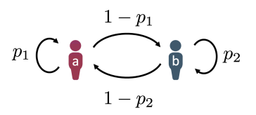
Figure 1: The simplified community network used to study community structure. Agent $a$ has bias parameter $\gamma$ and agent $b$ has bias parameter $1/\gamma$.

To analyze this network, we first find the equilibrium points.

Proposition 4.

The equilibrium points of the simplified community network are: ${\boldsymbol{0}}=(0,0)$; ${\boldsymbol{1}}=(1,1)$; and, when $\max\{\frac{p_{1}}{p_{2}},\frac{p_{2}}{p_{1}}\}<\gamma$, the interior equilibrium point ${\boldsymbol{\beta}}^{*}=(\beta_{a}^{*},\beta_{b}^{*})$ where

$$\beta_{a}^{*} =\frac{\gamma\left((\gamma+1)p_{1}p_{2}-2p_{2}+\sqrt{p_{1}p_{2}}\Delta\right)}{(\gamma-1)((\gamma+1)p_{1}p_{2}+\sqrt{p_{1}p_{2}}\Delta)}$$ (124)

$$\beta_{b}^{*} =\frac{2\gamma p_{1}-(\gamma+1)p_{1}p_{2}-\sqrt{p_{1}p_{2}}\Delta}{(\gamma-1)((\gamma+1)p_{1}p_{2}+\sqrt{p_{1}p_{2}}\Delta)}$$ (125)

where $\Delta=\sqrt{4\gamma(1-p_{1}-p_{2})+(\gamma+1)^{2}p_{1}p_{2}}\,.$  

Proof.

We solve the equation in Proposition 1. Then we check which of these solutions have $\beta_{a}$ and $\beta_{b}$ in $[0,1]$. ∎

To apply Theorem 1, we need the underlying adjacency matrix ${\boldsymbol{A}}={\boldsymbol{D}}{\boldsymbol{W}}$ to be symmetric. We choose

$${\boldsymbol{D}}=\begin{bmatrix}(1-p_{2})&0\\ 0&(1-p_{1})\end{bmatrix}$$ (126)

which results in a symmetric ${\boldsymbol{A}}$ (with the weight of the edge between $a,b$ set to $(1-p_{1})(1-p_{2})$ and the self-loops weights at $p_{1}(1-p_{2})$ and $p_{2}(1-p_{1})$, respectively). Then we apply Theorem 1 as desired to show that asymptotically the dynamics on the simplified community network almost surely converges to one of the equilibrium points. Next we determine under what conditions the dynamics asymptotically approaches consensus.

Proposition 5.

For the simplified community network,

$$\lim_{t\to\infty}{\boldsymbol{\beta}}(t)=\begin{cases}{\boldsymbol{\beta}}^{*}&\text{ if }\max\{\frac{p_{1}}{p_{2}},\frac{p_{2}}{p_{1}}\}<\gamma\\ {\boldsymbol{1}}&\text{ if }\gamma\leq\frac{p_{1}}{p_{2}}\\ {\boldsymbol{0}}&\text{ if }\gamma\leq\frac{p_{2}}{p_{1}}\end{cases}$$ (127)

almost surely where ${\boldsymbol{\beta}}^{*}$ is given by Proposition 4.

Proof.

We compute the eigenvalues of

$${\boldsymbol{J}}_{{\boldsymbol{0}}} =\begin{bmatrix}\gamma p_{1}&\gamma(1-p_{1})\\ \frac{1}{\gamma}(1-p_{2})&\frac{1}{\gamma}(p_{2})\end{bmatrix}\,.$$ (128)

The larger eigenvalue is given by

$$\lambda_{+}=\frac{1}{2}\left(\gamma p_{1}+\frac{p_{2}}{\gamma}\right)+\sqrt{\frac{1}{4}\left(\gamma p_{1}+\frac{p_{2}}{\gamma}\right)^{2}+1-p_{1}-p_{2}}\,.$$ (129)

and $\lambda_{+}<1$ exactly when $\gamma\leq\frac{p_{2}}{p_{1}}$. ∎

Note that these convergence results intuitively make sense, since if $p_{2}<p_{1}$, then agent $a$ reinforces her own opinion more by having more connections to herself. As agent $a$ has a bias towards opinion $1$, we expect $\beta_{a}(t)$ to be larger than $1/2$. If the proportion of edges agent $a$ has to herself compared to the proportion agent $b$ has to herself is much greater than $\gamma$, then agent $b$ will be overwhelmed by the pressure to conform.

By Theorem 3, when the conditions $\gamma\leq\frac{p_{1}}{p_{2}}$ or $\gamma\leq\frac{p_{2}}{p_{1}}$ do not hold, there are in fact no interior equilibrium points. This matches the conclusion of Proposition 4. Also, setting $p_{2}=1-p_{1}$ creates a system which behaves like the complete graph studied in [1]. The threshold for consensus given by Proposition 5 is consistent with that given in [1].

VI Conclusion

In this work, we studied the interacting Pólya urn model of opinion dynamics under social pressure. We expanded upon [1] by showing results for arbitrary networks and general bias parameters. To show that the probability of declared opinions converges asymptotically, we used an appropriate Lyapunov function and applied stochastic approximation, thus guaranteeing that in arbitrary networks, the behavior of agents almost surely converges. We also gave easily-computable necessary and sufficient conditions, for when the dynamics approach consensus. Our results provide insight as to how and when social pressure can force conformity of (expressed) opinions even against the true beliefs of some individuals.

The convergence and consensus results developed in this work have potential applications beyond this opinion dynamics model. These results may also apply to other social dynamics similar to the interacting Pólya urn model with non-linear interaction functions. A possible direction for further work is to find what consequences our techniques have for other models. Finding the interior equilibrium points for arbitrary networks is also an area for future work.

VI-A Inferring Inherent Beliefs

One of the key questions in [1] is whether it is possible to infer the inherent beliefs of agents from the history of declared opinions. This question was studied in [1] for the case of the complete graph using an aggregate estimator which keeps track of the overall ratio of $0$’s and $1$’s in the declared opinions of all agents throughout time. The results were that this estimator may not correctly estimate the inherent belief of all agents (even in the limit) if they approach consensus.

Unlike [1], our formulation also allows agents to have different honesty parameters. Thus, a natural question is how to estimate the honesty parameter (or, equivalently, the bias parameter) of any agent. Because we showed the behavior of agents almost surely converges in the limit, for large $t$ the values of $\mu_{i}(t)$ and $\beta_{i}(t)$ will be close to the equilibrium point. We can then use (41) to estimate the bias parameter $\gamma_{i}$ and inherent belief $\phi_{i}$ with

$$\widehat{\gamma}_{i}(t) =\frac{\beta_{i}(t)}{1-\beta_{i}(t)}\frac{1-\mu_{i}(t)}{\mu_{i}(t)}$$ (130)

$$\widehat{\phi}_{i}(t) ={\mathbb{I}}\{\beta_{i}(t)<\mu_{i}(t)\}$$ (131)

These estimators are asymptotically consistent, i.e.

$$\lim_{t\to\infty}\widehat{\gamma}_{i}(t) =\gamma_{i}$$ (132)

$$\lim_{t\to\infty}\widehat{\phi}_{i}(t) =\phi_{i}$$ (133)

when the dynamics converge to an interior equilibrium point (which is the regime where both $\lambda_{\max}({\boldsymbol{\Gamma}}{\boldsymbol{W}})>1$ and $\lambda_{\max}({\boldsymbol{\Gamma}}^{-1}{\boldsymbol{W}})>1$ as shown in Section IV.) However, plugging the equilibrium values into (130) is not well-defined if $\beta_{i}(t)$ and $\mu_{i}(t)$ both converge to either $0$ or $1$, i.e. when the dynamics converge to consensus. This shows that more careful analysis needs to be done in order to estimate the bias parameters and inherent beliefs in all circumstances, a direction for future work.

-B Stochastic Approximation Results

-B1 Generalized Pólya Urn Models

At any time $t$, let ${\boldsymbol{Z}}_{t}$ be the proportion of each color ball in the urn and ${\boldsymbol{b}}_{t}$ be the count of each color ball. The number of balls in the urn follows

$$b_{i,t+1}=b_{i,t}+\omega_{i,t}({\boldsymbol{Z}}_{t})\,$$ (134)

where ${\boldsymbol{q}}_{t}=(q_{1,t},\dots,q_{n,t})$ are the urn functions, and

$$\omega_{i,t}({\boldsymbol{z}})=\begin{cases}1&\text{ with probability }q_{i,t}({\boldsymbol{z}})\\ 0&\text{ with probability }1-q_{i,t}({\boldsymbol{z}})\end{cases}$$ (135)

for each $i=1,\dots,n$. The initial conditions are that ${\boldsymbol{b}}_{1}=(b_{1,1},\dots,b_{n,1})$ where $\zeta=\sum_{i=1}^{n}b_{i,1}$. Then

$$Z_{i,t+1} =Z_{i,t}+\frac{1}{\zeta+t}(\omega_{i,t}({\boldsymbol{Z}}_{t})-Z_{i,t})\,.$$ (136)

Theorem 4 (Theorem 3.1 from [26]).

Given continuous urn functions $\{q_{t}\}$, suppose there exists a Borel function $q:\Delta_{n-1}\to\Delta_{n-1}$, constants $\{a_{t}\}$ and a Lyapunov function $V:\Delta_{n-1}\to{\mathbb{R}}$ such that:

1. $\sup_{z\in\Delta_{n-1}}\|q_{t}(z)-q(z)\|\leq a_{t}$ where $\sum_{t=1}^{\infty}\frac{a_{t}}{t}<\infty$

2. The set $B=\{z:q(z)=z,z\in S\}$ contains a finite number of connected components

3. 1. $V$ is twice differentiable

   2. $V(z)\geq 0$ for $z\in\Delta_{n-1}$

   3. $\langle q(z)-z,\nabla V(z)\rangle<0$ for $z\in\Delta_{n-1}\setminus U(B)$ where $U(B)$ is an open neighborhood of $B$

then $\{z_{t}\}$ converges to a point of $B$ or to the border of a connected component.

The next two theorems are about stable and unstable points of the urn process. Given a point ${\boldsymbol{\theta}}$, we say that ${\boldsymbol{\theta}}$ is a stable point if there exists a symmetric positive-definite matrix ${\boldsymbol{C}}$ and a neighborhood $U$ of ${\boldsymbol{\theta}}$ such that

$$\langle{\boldsymbol{C}}({\boldsymbol{z}}-q({\boldsymbol{z}})),{\boldsymbol{z}}-{\boldsymbol{\theta}}\rangle>0$$ (137)

for ${\boldsymbol{z}}\neq{\boldsymbol{\theta}}$ and ${\boldsymbol{z}}\in U\cap S$. A point ${\boldsymbol{\theta}}$ is unstable if there exists a symmetric positive-definite matrix ${\boldsymbol{C}}$ and a neighborhood $U$ of ${\boldsymbol{\theta}}$ such that

$$\langle{\boldsymbol{C}}({\boldsymbol{z}}-q({\boldsymbol{z}})),{\boldsymbol{z}}-{\boldsymbol{\theta}}\rangle<0$$ (138)

for ${\boldsymbol{z}}\neq{\boldsymbol{\theta}}$ and ${\boldsymbol{z}}\in U\cap S$.

Theorem 5 (Theorem 5.1 from [26]).

Let ${\boldsymbol{\theta}}$ be a stable point in the interior of $S$. Given a process with transition functions $\{q_{n}\}$ which map the interior of $S$ into itself, and which converge in the sense that

$$\sup_{{\boldsymbol{z}}\in U\subset S}\|q_{n}({\boldsymbol{z}})-q({\boldsymbol{z}})\|\leq a_{n}$$ (139)

where $\sum_{n=1}^{\infty}a_{n}/n\leq\infty$, we then have

$${\mathbb{P}}[{\boldsymbol{Z}}_{n}\to{\boldsymbol{\theta}}]>0\,.$$ (140)

There is also a theorem for determining unstable interior equilibrium points.

Theorem 6 ([Theorem 5.2 from [26]).

For an interior unstable point ${\boldsymbol{\theta}}$ such that for all ${\boldsymbol{y}}$ in a neighborhood $U$ of ${\boldsymbol{z}}$,

$$\|F({\boldsymbol{y}},{\boldsymbol{\gamma}})-F({\boldsymbol{z}},{\boldsymbol{\gamma}})\|\leq c\|{\boldsymbol{y}}-{\boldsymbol{z}}\|^{\alpha}$$ (141)

for some constant $c$ and some $\alpha\in(0,1]$. Then

$${\mathbb{P}}[Z_{n}\to{\boldsymbol{\theta}}]=0\,.$$ (142)

-B2 Fitting Full Stochastic Model to Generalized Pólya Urn

In order to use the above theorems, we first need to show that our stochastic model fits within the class of generalized Pólya urn models. To verify this, recall that the full stochastic dynamics of our model (captured by (33) and (28)) is:

$$\beta_{i}(t+1) =\frac{t}{t+1}\beta_{i}(t)+\frac{1}{t+1}\psi_{i,t+1}$$ (143)

$$=\beta_{i}(t)+\frac{1}{t+1}\big{(}\psi_{i,t+1}-\beta_{i}(t)\big{)}$$ (144)

where

$$\psi_{i,t+1}\stackrel{{\scriptstyle\triangle}}{{=}}\left\{\begin{array}[]{lll}1&\text{w.p. }f\big{(}\frac{1}{\mathsf{deg}(i)}\sum_{j=1}^{n}a_{i,j}\beta_{j}(t),\gamma_{i}\big{)}\\ \\ 0&\text{w.p. }1-f\big{(}\frac{1}{\mathsf{deg}(i)}\sum_{j=1}^{n}a_{i,j}\beta_{j}(t),\gamma_{i}\big{)}\end{array}\right.\,$$ (148)

for all $i=1,\ldots,n$. This matches the update rules for the generalized Pólya urn model given by (135) and (136).

-C Local Stability

Using intuition from Lyapunov’s indirect method [29] (which is generally for continuous time problems) to our discrete problem, we would expect that vector ${\boldsymbol{x}}$ is locally stable if ${\boldsymbol{J}}_{{\boldsymbol{x}}}$ (defined in (71)) has all eigenvalues with real parts less than $1$, or equivalently, that ${\boldsymbol{J}}_{{\boldsymbol{x}}}-{\boldsymbol{I}}$ is a Hurwitz matrix. This intuition turns out to be correct, as shown by the statement of Proposition 3.

However, before proving Proposition 3, we first show that the eigenvalues of ${\boldsymbol{J}}_{{\boldsymbol{x}}}$ are in fact all real.

Lemma 5.

${\boldsymbol{J}}_{{\boldsymbol{x}}}$ has all real eigenvalues for any ${\boldsymbol{x}}\in[0,1]^{n}$.

Proof.

Using (71), we write that

$${\boldsymbol{J}}_{{\boldsymbol{x}}}={\boldsymbol{B}}{\boldsymbol{A}}$$ (149)

where ${\boldsymbol{B}}$ is a diagonal matrix with positive values on the diagonal and zeros elsewhere. Matrix ${\boldsymbol{A}}$ is the adjacency matrix of the (undirected) graph and hence is symmetric.

The matrix ${\boldsymbol{B}}^{1/2}$ is well-defined since ${\boldsymbol{B}}$ only has positive entries on the diagonal and the matrix ${\boldsymbol{B}}^{1/2}{\boldsymbol{A}}{\boldsymbol{B}}^{1/2}$ is symmetric, which means it has only real eigenvalues. Matrix ${\boldsymbol{J}}_{{\boldsymbol{x}}}$ is similar to

$${\boldsymbol{B}}^{-1/2}{\boldsymbol{J}}_{{\boldsymbol{x}}}{\boldsymbol{B}}^{1/2}={\boldsymbol{B}}^{1/2}{\boldsymbol{A}}{\boldsymbol{B}}^{1/2}$$ (150)

and similar matrices have the same eigenvalues. ∎

Proof of Proposition 3.

For the first statement, we need to show that for interior equilibrium point ${\boldsymbol{x}}$, if the eigenvalues of ${\boldsymbol{J}}_{{\boldsymbol{x}}}$ are less than $1$, there is some probability the opinions converge to ${\boldsymbol{x}}$. Let $\lambda=\lambda_{\max}({\boldsymbol{J}}_{{\boldsymbol{x}}})$. This proof primarily uses Theorem 5. In order to apply this, set ${\boldsymbol{C}}={\boldsymbol{I}}$ which is positive-definite. Then we have that

$$F({\boldsymbol{\beta}},{\boldsymbol{\gamma}})-F({\boldsymbol{x}},{\boldsymbol{\gamma}})=({\boldsymbol{J}}_{{\boldsymbol{x}}}+R({\boldsymbol{\beta}},{\boldsymbol{x}}))({\boldsymbol{\beta}}-{\boldsymbol{x}})$$ (151)

where $R({\boldsymbol{\beta}},{\boldsymbol{x}})\to 0$ as ${\boldsymbol{\beta}}\to{\boldsymbol{x}}$. Since $F({\boldsymbol{x}},{\boldsymbol{\gamma}})={\boldsymbol{x}}$,

$$F({\boldsymbol{\beta}},{\boldsymbol{\gamma}})-{\boldsymbol{\beta}} =({\boldsymbol{J}}_{{\boldsymbol{x}}}-{\boldsymbol{I}}+R({\boldsymbol{\beta}},{\boldsymbol{x}}))({\boldsymbol{\beta}}-{\boldsymbol{x}})$$ (152)

which implies

$$({\boldsymbol{\beta}}-{\boldsymbol{x}})^{{\scriptscriptstyle\top}} (F({\boldsymbol{\beta}},{\boldsymbol{\gamma}})-{\boldsymbol{\beta}})$$ (153)

$$=({\boldsymbol{\beta}}-{\boldsymbol{x}})^{{\scriptscriptstyle\top}}({\boldsymbol{J}}_{{\boldsymbol{x}}}-{\boldsymbol{I}})({\boldsymbol{\beta}}-{\boldsymbol{x}})$$

$$\quad\quad+({\boldsymbol{\beta}}-{\boldsymbol{x}})^{{\scriptscriptstyle\top}}(R({\boldsymbol{\beta}},{\boldsymbol{x}}))({\boldsymbol{\beta}}-{\boldsymbol{x}})$$ (154)

$$\leq(\lambda-1)\|{\boldsymbol{\beta}}-{\boldsymbol{x}}\|^{2}+\|R({\boldsymbol{\beta}},{\boldsymbol{x}})\|\|{\boldsymbol{\beta}}-{\boldsymbol{x}}\|^{2}$$ (155)

We can then choose $\|{\boldsymbol{\beta}}-{\boldsymbol{x}}\|$ small enough so that $\|R({\boldsymbol{\beta}},{\boldsymbol{x}})\|<1-\lambda$. This implies that

$$({\boldsymbol{\beta}}-{\boldsymbol{x}})^{{\scriptscriptstyle\top}}(F({\boldsymbol{\beta}},{\boldsymbol{\gamma}})-{\boldsymbol{\beta}})<0$$ (156)

This then gives that there exists a neighborhood $U$ around ${\boldsymbol{x}}$ so that for all ${\boldsymbol{\beta}}$

$$\langle {\boldsymbol{C}}({\boldsymbol{\beta}}-F({\boldsymbol{\beta}},{\boldsymbol{\gamma}})),{\boldsymbol{\beta}}-{\boldsymbol{x}}\rangle>0$$ (157)

and thus Theorem 5 shows that ${\boldsymbol{\beta}}(t)$ converges to ${\boldsymbol{x}}$ with some positive probability.

For the second statement, we apply Theorem 6. All we need to do is check that for interior equilibrium point ${\boldsymbol{x}}$,

1. There is a symmetric positive definite matrix ${\boldsymbol{C}}$ such that for any ${\boldsymbol{\beta}}\neq{\boldsymbol{x}}$ in a neighborhood $U$ of ${\boldsymbol{x}}$ we have

   $$\langle{\boldsymbol{C}}({\boldsymbol{\beta}}-F({\boldsymbol{\beta}},{\boldsymbol{\gamma}})),{\boldsymbol{\beta}}-{\boldsymbol{x}}\rangle<0\,.$$ (158)

2. and that for all ${\boldsymbol{\beta}}$ in a neighborhood $U$ of ${\boldsymbol{x}}$,

   $$\|F({\boldsymbol{\beta}},{\boldsymbol{\gamma}})-F({\boldsymbol{x}},{\boldsymbol{\gamma}})\|\leq c\|{\boldsymbol{\beta}}-{\boldsymbol{x}}\|^{\alpha}$$ (159)

   for some constant $c$ and some $\alpha\in(0,1]$.

For 1), let ${\boldsymbol{v}}$ be the corresponding eigenvector to $\lambda=\lambda_{\max}({\boldsymbol{J}}_{{\boldsymbol{x}}})$. Choose ${\boldsymbol{C}}={\boldsymbol{v}}{\boldsymbol{v}}^{{\scriptscriptstyle\top}}$. Then

$${\boldsymbol{C}}({\boldsymbol{J}}_{{\boldsymbol{x}}}-{\boldsymbol{I}})={\boldsymbol{v}}{\boldsymbol{v}}^{{\scriptscriptstyle\top}}({\boldsymbol{J}}_{{\boldsymbol{x}}}-{\boldsymbol{I}})=(\lambda-1){\boldsymbol{v}}{\boldsymbol{v}}^{{\scriptscriptstyle\top}}$$ (160)

which implies

$$({\boldsymbol{\beta}}-{\boldsymbol{x}})^{{\scriptscriptstyle\top}} {\boldsymbol{C}}({\boldsymbol{J}}_{{\boldsymbol{x}}}-{\boldsymbol{I}})({\boldsymbol{\beta}}-{\boldsymbol{x}})$$ (161)

$$=(\lambda-1)({\boldsymbol{\beta}}-{\boldsymbol{x}})^{{\scriptscriptstyle\top}}{\boldsymbol{v}}{\boldsymbol{v}}^{{\scriptscriptstyle\top}}({\boldsymbol{\beta}}-{\boldsymbol{x}})$$ (162)

$$=(\lambda-1)\langle{\boldsymbol{\beta}}-{\boldsymbol{x}},{\boldsymbol{v}}\rangle^{2}\geq 0$$ (163)

and thus 1) holds.

For 2), $F(\cdot,{\boldsymbol{\gamma}})$ is a continuous, twice differentiable and nonnegative function on a convex and compact domain. Let $C$ be the maximum magnitude of the gradient of $F({\boldsymbol{x}},{\boldsymbol{\gamma}})$ in any direction. The condition holds for $\alpha=1$ and $c=C\sqrt{n}$.

This shows that the dynamics cannot converge to this interior point. ∎

References

- [1] Ali Jadbabaie, Anuran Makur, Elchanan Mossel, and Rabih Salhab, “Inference in opinion dynamics under social pressure,” IEEE Transactions on Automatic Control, vol. 68, no. 6, pp. 3377–3392, 2023.
- [2] Hossein Noorazar, “Recent advances in opinion propagation dynamics: a 2020 survey,” The European Physical Journal Plus, vol. 135, no. 6, pp. 521, 2020.
- [3] Camilla Ancona, Francesco Lo Iudice, Franco Garofalo, and Pietro De Lellis, “A model-based opinion dynamics approach to tackle vaccine hesitancy,” Scientific Reports, vol. 12, no. 1, pp. 11835, 2022.
- [4] C. Miłosz, The Captive Mind, Knopf, 1953.
- [5] Solomon E. Asch, “Studies of independence and conformity: I. a minority of one against a unanimous majority,” Psychological monographs, vol. 70, no. 9, pp. 1–70, 1956.
- [6] Muzafer Sherif, “A study of some social factors in perception.,” Archives of Psychology (Columbia University), 1935.
- [7] Jr. French, John R. P., “A formal theory of social power,” Psychological review, vol. 63, no. 3, pp. 181–194, 05 1956.
- [8] Morris H. DeGroot, “Reaching a consensus,” Journal of the American Statistical Association, vol. 69, no. 345, pp. 118–121, 1974.
- [9] Noah E Friedkin and Eugene C Johnsen, “Social influence and opinions,” Journal of Mathematical Sociology, vol. 15, no. 3-4, pp. 193–206, 1990.
- [10] Rainer Hegselmann and Ulrich Krause, “Opinion dynamics and bounded confidence: models, analysis and simulation,” J. Artif. Soc. Soc. Simul., vol. 5, no. 3, 2002.
- [11] Guillaume Deffuant, Frédéric Amblard, Gérard Weisbuch, and Thierry Faure, “How can extremism prevail? a study based on the relative agreement interaction model,” Journal of artificial societies and social simulation, vol. 5, no. 4, 2002.
- [12] Claudio Altafini, “Consensus problems on networks with antagonistic interactions,” IEEE Transactions on Automatic Control, vol. 58, no. 4, pp. 935–946, 2013.
- [13] Peter Duggins, “A psychologically-motivated model of opinion change with applications to american politics,” Journal of Artificial Societies and Social Simulation, vol. 20, no. 1, pp. 13, 2017.
- [14] Pranav Dandekar, Ashish Goel, and David T. Lee, “Biased assimilation, homophily, and the dynamics of polarization,” Proceedings of the National Academy of Sciences, vol. 110, no. 15, pp. 5791–5796, 2013.
- [15] D. Kempe, J. Kleinberg, and É. Tardos, “Maximizing the spread of influence through a social network,” in Proceedings of the ninth ACM SIGKDD international conference on Knowledge discovery and data mining, 2003, pp. 137–146.
- [16] S. Bharathi, D. Kempe, and M. Salek, “Competitive influence maximization in social networks,” Internet and Network Economics, vol. 4858, pp. 306–311, 2007.
- [17] Arastoo Fazeli, Amir Ajorlou, and Ali Jadbabaie, “Competitive diffusion in social networks: Quality or seeding?,” IEEE Transactions on Control of Network Systems, vol. 4, no. 3, pp. 665–675, 2017.
- [18] H. Amini, M. Draief, and M. Lelarge, “Marketing in a random network,” Network Control and Optimization, vol. 5425, pp. 17–25, 2009.
- [19] Damon Centola, Robb Willer, and Michael Macy, “The emperor’s dilemma: A computational model of self‐enforcing norms,” American Journal of Sociology, vol. 110, no. 4, pp. 1009–1040, 2005.
- [20] Daron Acemoğlu, Giacomo Como, Fabio Fagnani, and Asuman Ozdaglar, “Opinion fluctuations and disagreement in social networks,” Mathematics of Operations Research, vol. 38, no. 1, pp. 1–27, 2013.
- [21] Jason Gaitonde, Jon Kleinberg, and Eva Tardos, “Adversarial perturbations of opinion dynamics in networks,” in Proceedings of the 21st ACM Conference on Economics and Computation, 2020, pp. 471–472.
- [22] Mengbin Ye, Yuzhen Qin, Alain Govaert, Brian D.O. Anderson, and Ming Cao, “An influence network model to study discrepancies in expressed and private opinions,” Automatica, vol. 107, pp. 371–381, 2019.
- [23] Abhimanyu Das, Sreenivas Gollapudi, Arindham Khan, and Renato Paes Leme, “Role of conformity in opinion dynamics in social networks,” in Proceedings of the second ACM conference on Online social networks, 2014, pp. 25–36.
- [24] Mikhail Hayhoe, Fady Alajaji, and Bahman Gharesifard, “Curing epidemics on networks using a polya contagion model,” IEEE/ACM Transactions on Networking, vol. 27, no. 5, pp. 2085–2097, 2019.
- [25] Somya Singh, Fady Alajaji, and Bahman Gharesifard, “A finite memory interacting polya contagion network and its approximating dynamical systems,” SIAM Journal on Control and Optimization, vol. 60, no. 2, pp. S347–S369, 2022.
- [26] W. Brian Arthur, Yu. M. Ermoliev, and Yu. M. Kaniovski, “Strong laws for a class of path-dependent stochastic processes with applications,” in Stochastic Optimization, Vadim I. Arkin, A. Shiraev, and R. Wets, Eds., Berlin, Heidelberg, 1986, pp. 287–300, Springer Berlin Heidelberg.
- [27] Henrik Renlund, “Generalized polya urns via stochastic approximation,” 2010.
- [28] Abraham Berman and Robert J. Plemmons, Nonnegative Matrices in the Mathematical Sciences, Society for Industrial and Applied Mathematics, 1994.
- [29] Hassan K. Khalil, Nonlinear Systems, Pearson Education. Prentice Hall, 2002.