A hybrid Decoder-DeepONet operator regression framework for unaligned observation data

Abstract

Deep neural operators (DNOs) have been utilized to approximate nonlinear mappings between function spaces. However, DNOs face the challenge of increased dimensionality and computational cost associated with unaligned observation data. In this study, we propose a hybrid Decoder-DeepONet operator regression framework to handle unaligned data effectively. Additionally, we introduce a Multi-Decoder-DeepONet, which utilizes an average field of the training data as input augmentation. The consistencies of the frameworks with the operator approximation theory are provided, on the basis of the universal approximation theorem. Two numerical experiments, Darcy problem and flow-field around an airfoil, are conducted to validate the efficiency and accuracy of the proposed methods. Results illustrate the advantages of Decoder-DeepONet and Multi-Decoder-DeepONet in handling unaligned observation data and showcase their potentials in improving prediction accuracy.

[inst1]organization=School of Aeronautics and Astronautics,addressline=Shanghai Jiao Tong University, city=Shanghai, postcode=200240, state=, country=China

[inst2]organization=School of Information Science and Engineering,addressline=Fudan University, city=Shanghai, postcode=200433, state=, country=China

Efficient Operator Regressions: Decoder-DeepONet and Multi-Decoder-DeepONet frameworks outperform traditional DNOs, enhancing accuracy and efficiency in handling unaligned data.

Input Augmentation Advancement: Multi-Decoder-DeepONet integrates averaged flow fields, boosting prediction accuracy in complex nonlinear mappings.

Consistent Operator Approximation: Hybrid frameworks maintain alignment with theory, combining decoder nets for improved handling of unaligned data problems.

1 Introduction

Computer-assisted artificial intelligence (AI) has become a powerful tool for solving a wide range of forward and inverse problems[1, 2, 3, 4, 5, 6, 7, 8, 9]. In recent years, building surrogate models to solve partial differential equations (PDEs) with deep neural networks (DNNs)[10, 11, 12, 13], such as convolutional neural networks (CNNs), recurrent neural networks (RNNs), long short-term memory networks (LSTMs), generative adversarial networks (GANs), and physics-informed neural networks (PINNs), has been achieved and tested to predict flow fields[7], compute chemical reactions[14], and solve protein folding problems[15], to name a few. The surrogate models may significantly reduce the computational cost once they are well-trained[2]. Most of the DNNs rely on the universal approximation theorem[16], which may approximate arbitrary functions with arbitrary accuracy. However, these models have limitations in accurately predicting the behavior of new systems subjected to different input signals, including boundary conditions, initial conditions, and source terms[17].

In contrast to DNNs that approximate functions, deep neural operators (DNO) are capable of approximating nonlinear mappings from an infinite function space to another, with the universal approximation theorem of operators providing the necessary mathematical guarantee [18]. The first framework of DNO was proposed by Lu et al. [17] in 2019, and named deep operator net (DeepONet). It consists of a branch net receiving function inputs and a trunk net receiving temporal and spatial observations. In 2020, Li et al. [19] formulated a new neural operator, Fourier neural operator (FNO), in which the integral kernel is directly parameterized in Fourier space. Both DeepONet and FNO have been demonstrated to learn operator mappings and forecast the evolution of systems with the variation of input signals[20]. DeepONet is more widely extended and utilized due to its flexible structure and small generalization errors. Using proper orthogonal decomposition (POD) to extract energetic modes in the trunk net, Lu et al. [20] further proposed a POD-DeepONet, in which the branch net is just utilized to learn the coefficients of the POD modes, resulting in less learning pressure and increased prediction accuracy. To extend the input function space from single to multiple, a multiple-input operator network (MIOnet)[21] consisting of more than one branch net was developed. Another impressive extension is physics-informed DeepONet[4], which provides a semi-supervised type of learning through a combination of PINNs and DeepONet. Further extensions of DeepOnet include multiple pre-trained DeepONets[22], DeepONet with uncertainty quantification[23], multiscale DeepONet[24], and others[25, 26]. DeepONet and its varieties have been applied in a broad range of applications, including the prediction of disturbance evolution in hypersonic boundary layers[27], the investigation of coupled flow and finite-rate chemistry in shock flow fields[28], the prediction of progressive intramural damage culminating in aortic dissection[29], and multiscale modeling of mechanical problems[30].

Two types of observation data, namely aligned and unaligned data, are usually encountered in academic studies and practical applications. The former represents that the physical coordinates of observations (outputs) are fixed under different input conditions. The unaligned data is formed when the distribution of the observations varies with the input conditions. For instance, the two-dimensional (2D) Darcy problem involves the mapping from a permeability field $k(\xi)$ to a pressure field $h(k)(\xi)$, where $\xi$ is the 2D observations $(\xi^{1},\xi^{2})$. This problem can be described using either aligned or unaligned data sets. Figure 1 illustrates the differences by using aligned and unaligned datasets. Figures 1($a,b$) display two distributions of the permeability fields $k_{1}$ and $k_{2}$, which are input conditions. Correspondingly, with the pressure fields observed with aligned dataset are shown in figures 1($c,d$), and those observed with unaligned dataset are shown in figures 1($e,f$). It can be seen that under different permeability fields as inputs, the observation locations of the pressure fields keep constant (uniformly distributed here) in figures 1($c,d$), but varies (randomly distributed) in figures 1($e,f$). Despite employing an identical number of observation points, the observed pressure fields ($h_{1}$ or $h_{2}$) differ due to disparities in the locations of observation points, which may significantly impact the learning of mappings from $k$ to $h$. Facing unaligned data, some DNNs, such as CNNs, lack the input of observation, which results in the learning of solely image-to-image mappings between initial conditions and results. Inherently, these approaches treat unaligned data as aligned data, disregarding the influences of observation points on the system variations.

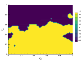
(a) $k_{1}(\xi)$

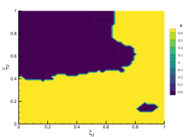
(b) $k_{2}(\xi)$

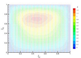
(c) $h_{1}(k_{1})(\xi)$-aligned

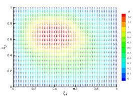
(d) $h_{2}(k_{2})(\xi)$-aligned

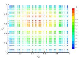
(e) $h_{1}(k_{1})(\xi)$-unaligned

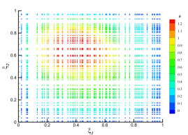
(f) $h_{2}(k_{2})(\xi)$-unaligned

Figure 1: The comparison of aligned and unaligned dataset. (a) A permeability field $k_{1}(\xi)$. (b) Another permeability field $k_{2}(\xi)$. (c) The pressure fields $h_{1}(k_{1})(\xi)$ corresponding to $k_{1}(\xi)$ with a uniform distribution of observations . (d) The pressure fields $h_{2}(k_{2})(y)$ corresponding to $k_{2}(\xi)$ with a uniform distribution. (e) $h_{1}(k_{1})(\xi)$ with a random distribution. (f) $h_{2}(k_{2})(\xi)$ with a random distribution.

Previous studies on DeepONet focused on the aligned data [20, 27, 28, 29, 30]. However, in specific application scenarios, the use of aligned data is not suitable for the development of surrogate models. For example, the aerodynamic shape optimization of airfoils, rotors, wings, and turbine blades involves the unaligned data problem, as the computational grids (flow field observations) vary with the shape configurations. Actually, the classical DeepONet[17] is able to handle both aligned and unaligned data through different data processing methodologies. To address the aligned data, CartesianProd implementation[20] is employed. Fundamentally, this implementation reuses the same set of trunk net input for all branch net inputs, reducing the training dataset size and computational redundancy. However, in the case of unaligned data, only the original prod implementation in Ref. [17] can be utilized, resulting in much larger dimensionality and more computational cost than those of aligned data. For high-dimensional unaligned observations, the exponentially increased dimensionality will challenge the network training, deteriorate the prediction accuracy, and heighten the memory requirements.

In this article, we propose a novel hybrid Decoder-DeepONet operator regression framework to handle the unaligned observation data. Additionally, a multiple input form named Multi-Decoder-DeepONet, inspired by MIOnet, is also effective, in which the average field of training data is fed into another subnetwork as input argumentation. We consider the prediction of Darcy problem and the prediction of flow-field around an airfoil to demonstrate the advantages of Decoder-DeepONet and Multi-Decoder-DeepONet compared with traditional networks. The paper is organized as follows. In Section 2, we provide a brief introdcution of the architecture and data evolution of DeepONet and its varieties and introduce the novel Decoder-DeepONet and Multi-Decoder-DeepONet operator regression framework. Comparative analysis of Decoder-DeepONet and Multi-Decoder-DeepONet against traditional DNOs is performed in Section 3. The conclusions are highlighted in Section 4.

2 Method

In this section, we give a concise introduction to the conventional approximation theory applied to both DeepONet and POD-DeepONet. Subsequently, we introduce the novel Decoder-DeepONet and Multi-Decoder-DeepONet operator regression and furnish the proof of the approximation theory.

2.1 The universal operator approximation theorem

The universal operator approximation theorem was first proposed by Chen and Chen [18]. Here we define an operator $G$ receiving the input function $u(x)$. At the observation points $\xi$ in the domain of $G(u)$, $G(u)(\xi)$ denotes the output field to be approximated.

Name that $K_{1}$ is a compact set in a Banach space, $K_{2}$ is a compact set in $\mathbb{R}^{d}$, $V$ is a compact set in $C(K_{1})$ which means the Banach space of all continuous functions defined on $K_{1}$ with norm $\|f\|_{C(K_{1})}=MAX_{x\in{K_{1}}}\mid f(x)\mid$. Then, the operator $G$ to be learned can be expressed as:

$${G}:V\ni{u}\mapsto G(u)(\xi)\in{C(K_{2})}.$$ (1)

Based on the study of Chen and Chen [18], the universal operator approximation theorem is given:

Theorem 1: For any small value $\epsilon>0$, there are positive integers n, p and m, $\sigma\in$ Tauber-Wiener (TW) functions, constants $c_{j}^{k}$, $\xi_{ij}^{k}$, $\theta_{i}^{k}$, $\zeta_{k}\in\mathbb{R}$, $w_{k}\in\mathbb{R}^{d}$, $x_{j}\in K_{1}$, $i=1,...,n$, $k=1,...,p$, and $j=1,...,m$, such that:

$$\left|G(u)(\xi)-\sum_{k=1}^{p}\sum_{i=1}^{n}c_{j}^{k}\sigma\left(\sum_{j=1}^{m}\xi_{ij}^{k}u(x_{j})+\theta_{i}^{k}\right)\sigma(w_{k}\cdot{\xi}+\zeta_{k})\right|<\frac{1}{2}\epsilon$$ (2)

holds for all $u\in V$ and $\xi\in K_{2}$, where $G:V\to C(K_{2})$ is the nonlinear continuous operator.

The universal operator approximation theorem suggests that a neural network containing at least one hidden layer is able to approximate any nonlinear continuous functional or operator. An architecture of operator neural network can be built to learn operator mappings from data, and the data-driven approach holds great potentials in a wide range of applications.

2.2 DeepONet

Lu et al. [17] extended the universal operator approximation theorem to a more general from. Considering two continuous vector functions $\textbf{b}(b_{1},...,b_{p}):\mathbb{R}^{m}\to\mathbb{R}^{p}$ and $\textbf{t}(t_{1},...,t_{p}):\mathbb{R}^{d}\to\mathbb{R}^{p}$, if we make $b_{k}(x)=\sum_{i=1}^{n}c_{j}^{k}\sigma\left(\sum_{j=1}^{m}\xi_{ij}^{k}x_{j}+\theta_{i}^{k}\right)$ and $t_{k}(\xi)=\sigma(w_{k}\cdot{\xi}+\zeta_{k})$, then Theorem 1 can be generalized as:

Theorem 2: For any $\epsilon>0$, there are $x_{j}\in K_{1}$, such that:

$$\left|G(u)(\xi)-\langle\textbf{b}(u(x_{1}),u(x_{1}),...,u(x_{m})),\textbf{t}(\xi)\rangle\right|<\frac{1}{2}\epsilon$$ (3)

holds for all $u\in V$ and $\xi\in K_{2}$, and $\langle\cdot,\cdot\rangle$ means the dot product. Essentially, Theorem 2 extends shallow networks in Theorem 1 to deep networks, which contain the activation function $\sigma\in$ TW functions to satisfy the classical universal approximation theorem of functional[31].

Based on Theorem 2, a network architecture of DeepONet[17] was developed to realize the operator mapping. Figure 2 shows the architecture of DeepONet. It consists of a branch net and a trunk net. Note that FNNs are used in the subnetwroks as an example. The branch net receives functional inputs u, encompassing initial conditions, boundary conditions, or source terms. The trunk net receives temporal or spatial observation coordinates $\xi$. With the dot product or Cartesian product (only for aligned data) operation, the output ${G}(u)(\xi)$ is approximated:

$${G}(\textit{u})(\xi)\approx\sum_{k=1}^{p}branch_{k}(\textit{u})\cdot trunk_{k}(\xi)+b_{0},$$ (4)

where $b_{0}$ is a bias to enhancing the representational capacity of the net. Note that the dimension evolution process for a two-dimensional aligned dataset is added in figure 2, making it different from the structure in Ref. [17]. For the aligned dataset, the function matrix and grid matrix have dimensions of $[N,k]$ and $[K,2]$ to be fed into the branch and trunk net, respectively. A Cartesian product of the subnet output matrices is performed to get the forecasting output matrix $G(u)(\xi)$. However, in the case of unaligned dataset, the dimension of function matrix and grid matrix will be $[N\times K,k]$ and $[N\times K,2]$, respectively. Instead of the Cartesian product, the forecasting output matrix $G(u)(\xi)$ will be obtained with a dot product operation of the two subnetwork output matrices, whose dimensions are $[N\times K,p]$. Obviously, the mapping relationship for the unaligned dataset is more complex compared to the aligned dataset. During the training process, the network for the unaligned dataset experiences greater learning pressure, with heavy consumption of computing and storage resources, which will challenge the network training to achieve a superior performance.

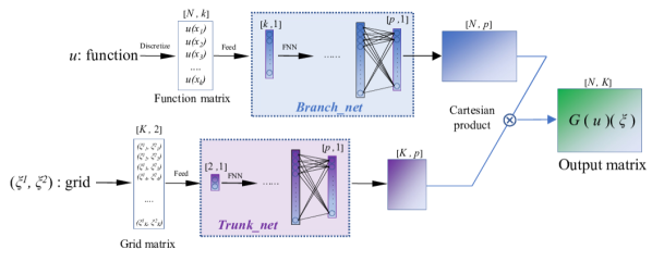
Figure 2: The architecture of DeepONet. Both branch net and trunk net are shown in the form of FNNs. The data fed into DeepONet is aligned here. $N$ is the number of input functions, each of which is dispersed by the $k$ points (u($x_{1}$),u($x_{2}$),u($x_{3}$) ….u($x_{k}$)); $K$ is the number of grid locations $\xi$ under each function $u$. To clearly display the datasize, $\xi$ in this paper is all shown as a 2D location $(\xi^{1},\xi^{2})$.

For the architecture of DeepONet, it is noteworthy to state that the explicit use of two independent subnetworks to handle information with different physical meanings itself is a form of embedded prior knowledge. Moreover, the network structures in the branch and trunk net are not restricted and may incorporate a wide range of structures, like FNNs, CNNs, and RNNs, making it flexible for different problems.

2.3 POD-DeepONet

Proper orthogonal decomposition (POD) is widely used to reduce the dimensionality of high-dimensional data while preserving the key features of the data[32]. It projects the high-dimensional data on low-rank basis functions, called POD modes, which characterize the dominant variability in the data. The coefficients of the POD modes represent the amplitude of the modes and can be used to reconstruct the original data.

In equation (4), the output function ${G}(u)(\xi)$ can be seen as a line combination of the branch and trunk net outputs. To improve the prediction accuracy of DeepONet, Lu et al. [20] proposed a POD-DeepONet, in which the pre-calculated POD modes are utilized in the trunk net, the branch net serves to learn the coefficients of the POD modes, and the Cartesian product operation is endowed with a similar operation to the POD reconstruction.

The architecture of the POD-DeepONet is shown in figure 3. Specifically, a Matrix splicing operation combines the output of the trunk net and the POD modes, giving a constraint condition that the dimension of the POD modes and the Grid matrix must be kept the same as each other. Although POD-DeepONet exhibits reduced learning pressure and superior accuracy, it can not train the unaligned data, as only one distribution of observation $\xi$ can be fed into the trunk net.

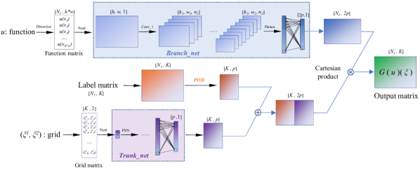
Figure 3: The architecture of POD-DeepONet. Branch net and trunk net are shown in the form of CNNs and FNNs, respectively. Only aligned data can be fed.

2.4 Decoder-DeepONet operator regression

Aiming to improve the prediction accuracy and efficiency of operator regression for unaligned data, we propose a hybrid Decoder-DeepONet operator regression framework, which is depicted in figure 4. Given the framework, the hybrid Decoder-DeepONet operator can be expressed as:

$$G(u)(\xi)\approx\underbrace{\boldsymbol{d}(}_{decoder}\underbrace{\boldsymbol{b}(\textit{u}(x_{1}),\textit{u}(x_{1}),...,\textit{u}(x_{k}))}_{branch},\underbrace{\boldsymbol{t}(\xi)}_{trunk}),$$ (5)

in which the explicit use of two independent subnetworks to handle information with different physical meanings is kept, whereas a decoder network $\boldsymbol{d}$ is used to merge the outputs of subnetworks instead of the dot product. More importantly, the decoder network allows that the varied observations at different input functions can be fed into the trunk net as a whole distribution, outperforming DeepONet and POD-DeepONet.

We will prove that the hybrid Decoder-DeepONet is also obeying the universal operator approximation theorem, sharing similarities of DeepONet in Theorem 2. Under the universal operator approximation theorem, we first prove that the dot product in DeepOnet can be replaced by a decoder network $\boldsymbol{d}$. Suppose that $\langle\bm{b},\bm{t}\rangle:\mathbb{R}^{2p}\to\mathbb{R}$ is the dot product function. The defined domain of $\langle\bm{b},\bm{t}\rangle$ is $\left\{\bm{b},\bm{t}\right\}$ = $\left\{b_{1},b_{2},...,b_{p},t_{1},t_{2},...,t_{p}\right\}$, being a compact set. Based on the universal approximation theorem of functional[31], the function $\langle\bm{b},\bm{t}\rangle$ is able to approximated by a decoder network, that is,

Theorem 3: For any $\epsilon>0$, there are $x_{j}\in K_{1}$, continuous vector functions $\bm{b}:\mathbb{R}^{m}\to\mathbb{R}^{p}$, $\bm{t}:\mathbb{R}^{d}\to\mathbb{R}^{p}$, $\bm{d}:\mathbb{R}^{2p}\to\mathbb{R}$, such that:

$$\left|\langle\bm{b}(u(x_{1}),u(x_{1}),...,u(x_{m})),\bm{t}(\xi)\rangle-\bm{d}(\bm{b},\bm{t})\right|<\frac{1}{2}\epsilon,$$ (6)

holds for all $u\in V$ and $\xi\in K_{2}$, where the decoder network $\bm{d}$ needs to satisfy the universal approximation theorem of functional, and all the notations above is shared from Theorem 2.

Substitute (6) into (3), we get:

Theorem 4: For any $\epsilon>0$, there are continuous vector functions $\bm{b}:\mathbb{R}^{m}\to\mathbb{R}^{p}$, $\bm{t}:\mathbb{R}^{d}\to\mathbb{R}^{p}$, $\bm{d}:\mathbb{R}^{2p}\to\mathbb{R}$, such that:

$$\left|G(u)(\xi)-\bm{d}(\bm{b}(u(x_{1}),u(x_{1}),...,u(x_{m})),\bm{t}(\xi))\right|<\epsilon,$$ (7)

holds for all $u\in V$ and $\xi\in K_{2}$.

Theorem 4 states that a decoder can serve as a substitute for the dot product operation utilized in DeepOnet. This operation will offer several advantages over DeepOnet:

(i) As an additional subnetwork, the decoder enhances the expressive power of the entire learning framework, enabling it to provide multidimensional outputs and facilitating efficient processing of unaligned data.

(ii) Regarding the dimension evolution of unaligned dataset in figure 4, the function matrix and grid matrix have the dimensions of $[N,k]$ and $[N,K,2]$ to be fed into the branch and trunk net, respectively. In contrast to DeepONet, which employs 2 neurons for receiving a single 2D observation to correspond with each function, Decoder-DeepOnet accommodates the $K$ of 2D observations to match every function by utilizing $K*2$ neurons, which significantly improves the efficiency of processing unaligned data. In figure 4, the $K$ observations can be reshaped into a structured shape of $H\times W$, offering a good choice of CNNs to learn the high-dimensional structured data.

(iii) Additionally, the outputs of the branch nets and trunk net are combined through splicing into different channels, which is the input of the decoder net to approximate the final output with the $K$ neurons in the last layer. Notably, besides the splicing operation to concatenate the outputs of subnetworks, addition and multiplication operation can also be utilized. Considering that the splicing operation preserves more dimensional and positional information and enables the subsequent layers of the decoder to choose features flexibly[33], we use it straightforwardly in the hybrid network.

When processing unaligned dataset as shown in figure 4, different from DeepOnet in which $\xi\in K_{2}\subset\mathbb{R}^{d}$, $\xi$ in the grid matrix of Decoder-DeepONet can be a vector of $K\cdot d$ dimensions in $\mathbb{R}^{K\cdot d}$ ($K$=$H*W$, $d$=2 in figure 4). Similarly, $G$ in the output matrix of Decoder-DeepONet is a vector of $K$ dimensions. It can be considered as a special case of Theorem 4 in which we feed the observation coordinate $\xi$ with dimensions of $h\cdot d$ and get the output $G$ with dimensions of $h$. So Theorem 4 still holds with $\bm{t}:\mathbb{R}^{h*d}\to\mathbb{R}^{p}$ and $\bm{d}:\mathbb{R}^{2p}\to\mathbb{R}^{h}$.

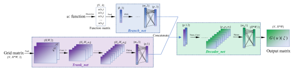
Figure 4: The architecture of hybrid Decoder-DeepOnet operator regression framework. The dimension evolution of unaligned dataset is processed in this figure. Note that H*W in this figure is numerically equal to K in Figure 2 and 3. We specifically select the use of H*W over K here to illustrate that CNNs are a viable choice if the input data is structured.

For the loss function, the mean squared error (MSE) is adopt to measure the square of L2 norm between predictions and true values. Given the data size in figure 4, the loss is expressed as:

$$\mathcal{L}=\frac{1}{N\cdot H\cdot W}\sum\limits_{i=1}^{N}\sum\limits_{j=1}^{H\cdot W}(G_{model}(\textit{u}_{i})(\xi_{j})-G_{truth}(\textit{u}_{i})(\xi_{j}))^{2},$$ (8)

where $G_{truth}(\textit{u}_{i})(\xi_{j})$ means the ground-truth data under the i-th input function at j-th observation point and $G_{truth}(\textit{u}_{i})(\xi_{j})$ is the corresponding output of the model learnt by Decoder-DeepOnet.

2.5 Multi-Decoder-DeepOnet with input augmentation

Drawing inspiration from the multiple-input operator[21], Decoder-DeepOnet can be easily extended to a multiple-input form. In this study, we provide a Multi-Decoder-DeepOnet, which incorporates an input augmentation to further improve the prediction accuracy of operator regression.

Fruitful prior knowledge is hiding in the label data. Here we utilize the mean field of the label data as an input augmentation to incorporate the information of the known label data. The mean field of the label data is expressed as,

$$\overline{G}=\frac{1}{N}\sum\limits_{i=1}^{N}G_{i}(u_{i})(\xi),$$ (9)

where $N$ is the number of the output functions in training data.

The architecture of the Multi-Decoder-DeepOnet is shown in figure 5. A branch-average-net is added to receive the mean field of the label data. The branch-average-net is responsible for extracting features in the mean field, providing a warm start for operator learning. Owning to the decoder net’s flexibility, the information in the branch-average-net can be integrated and decoded to generate the corresponding field data.

Figure 5: The architecture of hybrid Multi-Decoder-DeepOnet operator regression framework.

Given the framework in figure 5, the Multi-Decoder-DeepONet can be expressed as:

$$G(u)(\overline{G})(\xi)\approx\underbrace{\boldsymbol{d}(}_{decoder}\underbrace{\boldsymbol{b}(\textit{u}(x_{1}),\textit{u}(x_{1}),...,\textit{u}(x_{k}))}_{branch},\underbrace{\boldsymbol{b}_{a}(\overline{G})}_{branch_{a}},\underbrace{t(\xi)}_{trunk}),$$ (10)

where $\boldsymbol{b}_{a}$ represents the branch-average-net.

The approximation theory of Multi-Decoder-DeepONet with input augmentation is given as,

Theorem 5: For any $\epsilon>0$, there are $x_{j}\in K_{1}$, $\bm{b_{1}}:\mathbb{R}^{m}\to\mathbb{R}^{p}$, $\bm{b_{2}}:\mathbb{R}^{h}\to\mathbb{R}^{p}$, $\bm{f}:\mathbb{R}^{h\cdot d}\to\mathbb{R}^{p}$, $\bm{d}:\mathbb{R}^{3p}\to\mathbb{R}^{h}$, such that :

$$\left|G(u)(\overline{G})(\xi)-\bm{d}(\bm{b_{1}}(u(x_{1}),u(x_{1}),...,u(x_{m})),\bm{b_{2}}(\overline{G}),\bm{t}(\xi))\right|<\epsilon,$$ (11)

holds for all $u\in V$ and $\xi\in K_{2}$. The proof is referred to the study of Jin et al. [21], in which the approximation theory for multiple-input operator regression was first proposed.

Similar to to Decoder-DeepONet, the loss in the training of Multi-Decoder-DeepONet is given as,

$$\mathcal{L}=\frac{1}{N*H*W}\sum\limits_{i=1}^{N}\sum\limits_{j=1}^{H*W}(G_{model}(\textit{u}_{i})(\overline{G})(\xi_{j})-G_{truth}(\textit{u}_{i})(\overline{G})(\xi_{j}))^{2}.$$ (12)

3 Numerical experiments

Two numerical experiments are provided here to demonstrate the efficiency and accuracy of the proposed methods. The network training is performed on NVIDIA GeForce RTX 3090 GPU. All codes and data can be found in GitHub at github_Deocer_DeepONet, which are developed on the basis of DEEPXDE[34], a library for scientific machine learning, with Tensorflow as the backend.

3.1 Two-dimensional Darcy flows

The Darcy flow is a benchmark problem for operator learning. In previous studies[19, 20], only aligned datasets of the Darcy problem have been tested. Here we focus on the superiority of Decoder-DeepOnet and Multi-Decoder-DeepOnet for unaligned data, in terms of learning accuracy and memory usage, compared to the basic DeepONet.

3.1.1 Problem setup

The governing equations of two-dimensional Darcy flows are linear elliptic PDEs[20],

$$\left\{\begin{array}[]{cc}-\bigtriangledown\cdot(k(\xi^{1},\xi^{2})\bigtriangledown h(\xi^{1},\xi^{2}))=f,\\ h(\xi^{1},\xi^{2})=0,\end{array}\right.$$ (13)

where $(\xi^{1},\xi^{2})$ is the spatial coordinates, $k$ and $h$ denote the permeability and pressure field, respectively, and $f$ is a forcing function which can be either a constant or a function. Here the forcing is fixed as $f$ = 1.

The permeability field denoted by $k$ is mathematically defined as $k=\psi(\mu)$, where the random variable $\mu$ corresponds to the Gaussian random field with zero Neumann boundary conditions on the Laplacian and is evaluated at points $\mu=R(0,(-\bigtriangleup+9I)^{-2})$. The push-forward of the mapping $\psi$ is defined pointwise, with a value of 12 assigned to the positive segment of the real line and 3 assigned to its negative counterpart.

The target is to learn the operator mapping from the permeability field $K(\xi)$ to the pressure field $h(k)(\xi)$:

$$\mathcal{G}:K(\xi)\mapsto h(k)(\xi).$$ (14)

3.1.2 Data generation

A rectangular domain is set with $(\xi^{1},\xi^{2})\in{(0,1)}$. The data set for training and testing is generated using the MATLAB Partial Differential Equation Toolbox[19]. Notably, the grids $\xi$ for each different $h(k)$ is sampled randomly via different seeds to generate unaligned data like Figure 1. Three kinds of cases with different resolutions ($29\times 29,43\times 43,61\times 61$) are used here to eliminate the impact of sampling resolution.

In the training process, $k(\xi)$ and the averaged pressure filed $\overline{h}$ are fed into the branch net and branch-average-net, respectively. The trunk net receives the gird distributions. Finally, $h(\xi)$ is operated as the ground-truth data to estimate the loss of the operator approximation, which is defined in section 2.2. In general, 1000 samples are selected randomly for training, and 200 samples are used to evaluate the capabilities of the trained models concerning generalization.

Table 1 shows the data size comparison between DeepONet and Decoder-DeepOnet for unaligned data. It is evident that for identical resolution data, the Decoder-DeepOnet dataset encapsulates training information more efficiently than DeepONet. The data redundancy in DeepONet is primarily attributable to the function matrix, in which the same function repeatedly matches each single observation point. It should be noted that the data of Multi-Decoder-DeepOnet includes only one additional label-average matrix of identical size to the function matrix of Decoder-DeepOnet, compared to Decoder-DeepOnet data. As POD-DeepONet is incapable of managing unaligned data, it is omitted for comparison.

Table 1: Training data size of DeepONet and Multi-Decoder-DeepOnet for the unaligned Darcy problem

Case	Method	Resolution of $k$	Function matrix	Gird matrix	Output matrix
case-1	DeepONet	29*29	[1000*841, 841]	[1000*841,2]	[1000*841,1]
case-2	Decoder-DeepOnet	29*29	[1000, 841]	[1000,841,2]	[1000,841]
case-3	DeepONet	43*43	[1000*1849, 1849]	[1000*1849,2]	[1000*1849,1]
case-4	Decoder-DeepOnet	43*43	[1000, 1849]	[1000,1849,2]	[1000,1849]
case-5	DeepOnet	61*61	[1000*3721,841]	[1000*3721,2]	[1000*3721,1]
case-6	Decoder-DeepOnet	61*61	[1000, 841]	[1000,3721,2]	[1000,3721]

3.1.3 Results

As the input datasets of the subnetworks exhibit structured characteristics, we employ CNNs, incorporating pooling layers and a fully connected layer in the final stage, to facilitate superior feature extraction from the permeability field, the average pressure field and the grid distribution. FNNs are employed in the decoder net here.

The specific hyperparameters of Decoder-DeepOnet and Multi-Decoder-DeepOnet are displayed in A. The sets of DeepONet are the same as Ref. [17]. We train the models using the Adam optimizer[35] with a learning rate of 1e-5.

The training and testing errors are listed in Table 2. It can be seen that, regardless of the grid resolutions, Decoder-DeepONet performs better than DeepONet in reducing the training and testing errors for the unaligned data, and superior performance is achieved by Multi-Decoder-DeepONet with input augmentation.

Given the enhanced descriptiveness of the output function with increased observations, the impact of observation distribution is mitigated for high-resolution data compared to low-resolution data. This assertion is corroborated by the data presented in Table 2, which illustrates that superior learning performance is consistently achieved at higher resolutions, irrespective of the methodology employed, and the improvement in learning accuracy brought about by Decoder-DeepONet and Multi-Decoder-DeepONet is markedly significant at lower resolutions.

It is pertinent to note, however, that the observational distribution utilized in the experiments is randomly generated, devoid of physical significance or systematic patterns, thus rendering the trunk net incapable of effectively mapping the observation input to a low-dimensional latent space. Consequently, despite the substantial enhancements achieved with the Decoder-DeepONet and Multi-Decoder-DeepONet, prediction accuracy remains somewhat limited. To further illustrate the superiority of the proposed frameworks, the following experiment will explore a natural unaligned airfoil flow field problem.

Table 2: MSE loss of DeepONet, Decoder-DeepONet and Multi-Decoder-DeepONet for the Darcy problem

case	method	resolution	training error	testing error
case-1	DeepONet	29*29	2.71e-02	3.61e-02
case-2	Decoder-DeepOnet	29*29	4.35e-03	1.23e-02
case-3	Multi-Decoder-DeepOnet	29*29	5.53e-03	8.98e-03
case-4	DeepONet	43*43	2.95e-02	3.62e-02
case-5	Decoder-DeepOnet	43*43	3.14e-03	1.03e-02
case-6	Multi-Decoder-DeepOnet	43*43	3.95e-03	7.73e-03
case-7	DeepOnet	61*61	2.76e-02	2.33e-02
case-8	Decoder-DeepOnet	61*61	3.13e-03	7.48e-03
case-9	Multi-Decoder-DeepOnet	61*61	2.17e-03	6.53e-03

3.2 Prediction of the flow-field around an airfoil

The prediction of the flow-field around an airfoil is always achieved by solving Navier-Stokes equations, which will consume high computing cost with traditional computational fluid dynamics (CFD) methods[36].

Alternatively, fast surrogate models with DNNs have been used for the flow-field predictions[37, 38, 39, 40, 41, 42]. Different airfoil shapes (wall boundary conditions) corresponds to different the flow-fields around the airfoils (observations). It is a natural unaligned problem as the observation distributions (computational grids) vary in accordance with the airfoil shapes. Most previous studies did not account for the influence of unaligned data (mesh non-uniformity). Recently the learning of operators makes up the deficiencies[43, 44], but still face challenges in network training.

Here we use this unaligned problem to demonstrate the capability and efficiency of Decoder-DeepONet and Multi-Decoder-DeepONet in learning operators of unaligned data compared with DeepONet. Additionally, to underscore the significance of accommodating unaligned observations, we also conduct experiments using DeepONet and POD-DeepONet methods to learn the unaligned data in an aligned manner, namely, by feeding only a uniform observation distribution into the trunk net. The specific problem set up and data generation are described below.

3.2.1 Problem setup

Focusing on the pressure distributions around the airfoil, the ground truth data for training and testing is generated from the simulation of compressible Reynolds-averaged Navier-Stokes (RANS) equations. We consider the flow condition: Reynolds number $Re=3\times{10^{6}}$, the incoming flow Mach number $Ma=0.5$ and the angle of attack being $2.5^{\circ}$.

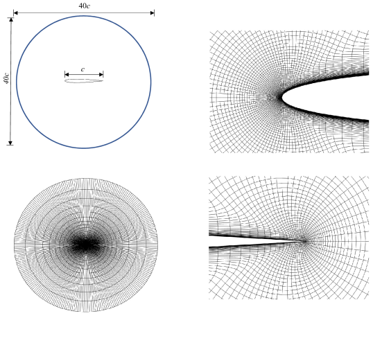
Figure 6: The computational grids.

3.2.2 Data generation

The CFD is performed with an open source code $CFL3D$ [45], and all solutions are calculated using k-$\omega$ SST two equation turbulence model. The validation is provided in B. A shape space containing 200 airfoils, which varies from NACA0005 to NACA5535, is generated. The O-shaped structured grids shown in figure 6 are automatically generated by using scripts of pyGlyph based on python. To eliminate the influence of boundaries on the flow field, we set the chord length of the O-type computational domain to $20c$ and $c$ is the chord length of airfoils. The grid matrix shape of the computational domain is $241\times 120$ and a $241\times 100$ internal area is selected for the network training.

In the training process, the airfoil shape is represented by 256 grid points and fed into the branch net directly without independent parameter dimensionality reduction. The branch net receives the airfoil shapes as the wall boundary conditions, and the $241\times 100$ mesh grids are fed into the trunk net. The pressure distributions obtained by CFD method are regarded as the ground-truth data to examine the loss of the operator approximation, which is defined in section 2.

Table 3: MSE loss of the flow-filed around the airfoil

case	method	resolution	training error	testing error
case-1	DeepONet	121*100	5.87e-04	1.83e-02
case-2	DeepONet (aligned method)	121*100	5.53e-05	8.44e-05
case-3	POD-DeepONet (aligned method)	121*100	8.20e-07	4.49e-07
case-4	Decoder-DeepOnet	121*100	3.60e-07	4.11e-07
case-5	Multi-Decoder-DeepOnet	121*100	5.43e-08	1.67e-07

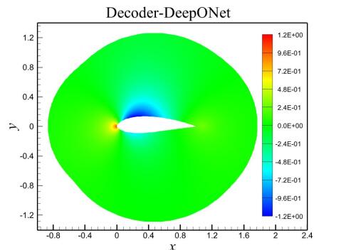
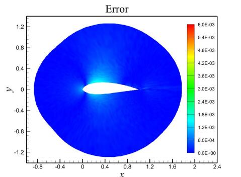
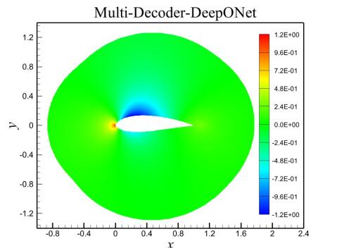
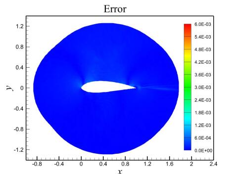
Figure 7: The predicted pressure coefficients and the absolute errors around a randomly selected airfoil from the testing set

3.2.3 Results

We compare Decoder-DeepOnet and Multi-Decoder-DeepOnet with other three classical operator methods: DeepONet with real unaligned observations, DeepONet with aligned uniform observations and POD-DeepONet with aligned uniform observations. Details of the hyperparameters are provided in C. We train the models using the Adam optimizer[35] with a learning rate of 1e-4. The resultant mean squared errors, during training and testing, are listed in Table 3.

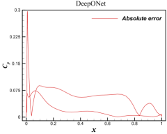
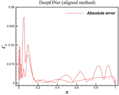
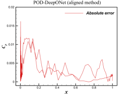
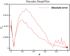
Figure 8: The absolute errors between the truth and prediction of pressure coefficients distribution on the airfoil surface.

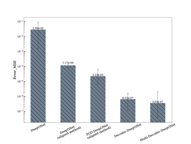
Figure 9: The MSE errors of all testing cases on the airfoils surface.

First, the performance of DeepONet using unaligned observations exhibits suboptimal results. As the closest comparison, DeepONet utilizing aligned observations shows lower errors, particularly in terms of testing errors. The underperformance of the former can be attributed to the more intricate mapping relationship to be learned and the vast quantity of training data employed. However, expanding the network structure in terms of depth and width does not alleviate this situation. Implementation of the POD-DeepONet leads to reduced learning pressure and improved accuracy. Although the POD-DeepONet and DeepONet with aligned observations benefit from a simpler mapping relationship and smaller training dataset size, it is not physically justifiable to consider unaligned data as aligned.

As for Decoder-DeepONet and Multi-Decoder-DeepONet, the prediction errors are several orders of magnitude lower than other methods, and Multi-Decoder-DeepONet with input augmentation delivers the most superior performance. With receiving real unaligned observations, Decoder-DeepONet and Multi-Decoder-DeepONet process data in a more efficient way without a significant increase of the training data size.

Figure 7 illustrates the predicted pressure coefficients and the absolute errors around a randomly selected airfoil from the testing set. It can be seen that Decoder-DeepONet and Multi-Decoder-DeepONet substantially outperform the other methods in predicting the flow field. Notably, the flow field predicted by Multi-Decoder-DeepONet aligns well with the true flow field. In addition, the prediction errors are predominantly localized near the wall surface, where fine grid distribution and considerable gradients of pressure change impact the aerodynamic performance of the airfoil.

Figure 8 shows the absolute errors between the truth and predicted pressure coefficients on the wall surface. The predictions of DeepONet using unaligned method have the worst agreement with the truth values, as expected. Reductions of the errors are observed for DeepONet and POD-DeepONet using the alignment method. In contrast, Decoder-DeepONet and Multi-Decoder-DeepONet reduce the errors significantly, especially for Multi-Decoder-DeepONet. Figure 9 shows the MSE errors of pressure coefficients on the wall surface for all test cases, quantitively illustrate the advantages of Decoder-DeepONet and Multi-Decoder-DeepONet over the other methods.

In summary, incorporating decoder nets, Decoder-DeepONet receives physical grid coordinates in the trunk net, which involving the non-uniformity of the grid in the near-wall region. Multi-Decoder-DeepONet further includes the averaged flow field as an input enhancement. Results demonstrate the superiority of the new methods in handling the unaligned observation data.

4 Conclusions

In this study, we propose a hybrid Decoder-DeepONet operator regression framework, and extend it to the Multi-Decoder-DeepONet by incorporating an input augmentation. Two numerical experiments are performed to evaluate the efficiency and accuracy of the proposed methods. Conclusions are summarized below:

(i) Replacing the dot product by a decoder net, Decoder-DeepONet still obeys the operator approximation theory. It can be easily extended to an input-augmentation form, due to the flexibility of the decoder net. We give Multi-Decoder-DeepONet, which utilizes the mean field of the label data as the input augmentation.

(ii) In comparison with the classical forms of DeepONet, the proposed methods are validated to be more efficient and accurate in the operator regression of unaligned data problems. The improvements may contribute to a broader understanding of operator approximation and accelerate the practical applications in various fields.

Declaration of competing interest

The authors declare that they have no known competing financial interests or personal relationships that could have appeared to influence the work reported in this paper.

Declaration of generative AI in scientific writing

During the preparation of this work the authors used Chatgpt4 in order to improve readability. After using this tool/service, the authors reviewed and edited the content as needed and take full responsibility for the content of the publication

APPENDIX A Hyperparameters in the Darcy problem

Here we list the hyperparameters of the networks with the best performance in the Darcy problem. Table 4, 5 and 6 show the hyperparameters of DeepONet, Decoder-DeepONet and Multi-Decoder-DeepONet, respectively.

Table 4: Hyperparameters of DeepONet

subnet	Layer	Input Shape	Output Shape	Activation	Filters	Filter Size	Stride Size
Branch-net	Conv2D	61x61x1	29x29x64	ReLU	64	5x5	2
	Conv2D	29x29x64	13x13x128	ReLU	128	5x5	2
	Flatten	13x13x128	204928	-	-	-	-
	Dense	204928	256	ReLU	-	-	-
	Dense	256	256	None	-	-	-
Trunk-net	Dense	2	256	ReLU	-	-	-
	Dense	256	512	ReLU	-	-	-
	Dense	512	512	ReLU	-	-	-
	Dense	512	256	None	-	-	-

Table 5: Hyperparameters of Decoder-DeepONet

subnet	Layer	Input Shape	Output Shape	Activation	Filters	Filter Size	Stride Size
Branch-net	Conv2D	61x61x1	29x29x16	ReLU	16	5x5	2
	Conv2D	29x29x16	13x13x8	ReLU	8	5x5	2
	Flatten	13x13x8	128	-	-	-	-
	Dense	128	200	None	-	-	-
Trunk-net	Conv2D	61x61x1	29x29x16	ReLU	16	5x5	2
	Conv2D	29x29x16	13x13x8	ReLU	8	5x5	2
	Flatten	13x13x8	128	-	-	-	-
	Dense	128	200	None	-	-	-
Dot-net	Flatten	2x200	400	-	-	-	-
	Dense	400	1000	ReLU	-	-	-
	Dense	1000	3721	None	-	-	-

Table 6: Hyperparameters of Multi-Decoder-DeepONet

subnet	Layer	Input Shape	Output Shape	Activation	Filters	Filter Size	Stride Size
Branch-net	Conv2D	61x61x1	29x29x16	ReLU	16	5x5	2
	Conv2D	29x29x16	13x13x8	ReLU	8	5x5	2
	Flatten	13x13x8	1352	-	-	-	-
	Dense	1352	128	ReLU	-	-	-
	Dense	128	20	None	-	-	-
Branch-average-net	Conv2D	61x61x1	29x29x16	ReLU	16	5x5	2
	Conv2D	29x29x16	13x13x8	ReLU	8	5x5	2
	Flatten	13x13x8	1352	-	-	-	-
	Dense	1352	128	ReLU	-	-	-
	Dense	128	20	None	-	-	-
Trunk-net	Conv2D	61x61x1	29x29x16	ReLU	16	5x5	2
	Conv2D	29x29x16	13x13x8	ReLU	8	5x5	2
	Flatten	13x13x8	1352	-	-	-	-
	Dense	1352	128	ReLU	-	-	-
	Dense	128	20	None	-	-	-
Dot-net	Flatten	3x20	60	-	-	-	-
	Dense	60	500	ReLU	-	-	-
	Dense	500	3721	None	-	-	-

APPENDIX B Validation of CFD Method

We utilize the experimental data of the RAE2822 Airfoil[46] to validate the accuracy of the CFD simulaiton employed in this study. The test conditions comprise a Mach number of 0.75, a Reynolds number of 6.5 million, and an angle of attack of 2.92 degrees. Figure 10 shows the comparison of the CFD results and the experimental data. It can be seen that the simulated results have good agreements with the experimental data.

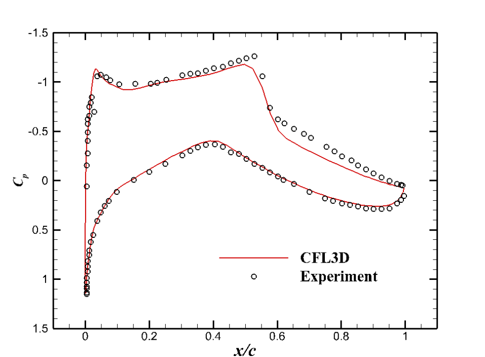
Figure 10: The comparison of CFD results and experimental data

APPENDIX C Hyperparameters in the prediction of flow-field around an airfoil

Here we list the hyperparameters of the networks with best performance, which are used in the prediction of flow-field around an airfoil. Talble 7, 8, 9, 10 and 11 show the hyperparameters of DeepONet, DeepONet (aligned method), POD-DeepONet (aligned method), Decoder-DeepONet and Multi-Decoder-DeepONet, respectively.

Table 7: Hyperparameters of DeepONet

subnet	Layer	Input Shape	Output Shape	Activation	Filters	Filter Size	Stride Size
Branch-net	Conv2D	32x16x1	14x6x64	ReLU	64	5x5	2
	Conv2D	14x6x32	5x1x128	ReLU	128	5x5	2
	Flatten	5x1x128	640	-	-	-	-
	Dense	640	128	ReLU	-	-	-
	Dense	128	200	None	-	-	-
Trunk-net	Dense	2	256	ReLU	-	-	-
	Dense	256	256	ReLU	-	-	-
	Dense	256	200	None	-	-	-

Table 8: Hyperparameters of DeepONet (aligned method)

subnet	Layer	Input Shape	Output Shape	Activation	Filters	Filter Size	Stride Size
Branch-net	Dense	256	512	ReLU	-	-	-
	Dense	512	1024	ReLU	-	-	-
	Dense	1024	1024	ReLU	-	-	-
	Dense	1024	512	ReLU	-	-	-
	Dense	512	128	None	-	-	-
Trunk-net	Dense	2	256	ReLU	-	-	-
	Dense	256	256	ReLU	-	-	-
	Dense	256	128	None	-	-	-

Table 9: Hyperparameters of POD-DeepONet (aligned method)

subnet	Layer	Input Shape	Output Shape	Activation	Filters	Filter Size	Stride Size
Branch-net	Conv2D	32x16x1	14x6x64	ReLU	64	5x5	2
	Conv2D	14x6x32	5x1x128	ReLU	128	5x5	2
	Flatten	5x1x128	640	-	-	-	-
	Dense	640	128	ReLU	-	-	-
	Dense	128	128	None	-	-	-
Trunk-net	Dense	2	128	ReLU	-	-	-
	Dense	128	64	None	-	-	-
Number of POD modes: 64

Table 10: Hyperparameters of Decoder-DeepONet

subnet	Layer	Input Shape	Output Shape	Activation	Filters	Filter Size	Stride Size
Branch-net	Conv2D	32x16x1	14x6x32	ReLU	32	5x5	2
	Conv2D	14x6x32	5x1x16	ReLU	16	5x5	2
	Flatten	5x1x16	80	-	-	-	-
	Dense	80	200	None	-	-	-
Trunk-net	Conv2D	100x241x2	33x79x32	ReLU	32	3x5	3
	Conv2D	33x79x32	11x25x16	ReLU	16	3x5	3
	Flatten	11x25x16	4400	-	-	-	-
	Dense	4400	200	None	-	-	-
Dot-net	Conv2D-Transpose	2x200x1	10x1000x64	ReLU	64	2x2	5
	Conv2D	10x1000x64	10x1000x1	ReLU	1	1x1	1
	Flatten	10x1000x1	10000	-	-	-	-
	Dropout	10000	10000	-	-	-	-
	Dense	10000	24100	None	-	-	-

Table 11: Hyperparameters of Multi-Decoder-DeepONet

subnet	Layer	Input Shape	Output Shape	Activation	Filters	Filter Size	Stride Size
Branch-net	Conv2D	32x16x1	14x6x32	ReLU	32	5x5	2
	Conv2D	14x6x32	5x1x16	ReLU	16	5x5	2
	Flatten	5x1x16	80	-	-	-	-
	Dense	80	200	None	-	-	-
Branch-average-net	Conv2D	100x241x1	48x119x32	ReLU	32	5x5	2
	Conv2D	48x119x32	22x58x16	ReLU	16	5x5	2
	Flatten	22x58x16	20416	-	-	-	-
	Dense	20416	200	None	-	-	-
Trunk-net	Conv2D	100x241x2	48x119x32	ReLU	32	5x5	2
	Conv2D	48x119x32	22x58x16	ReLU	16	5x5	2
	Flatten	22x58x16	20416	-	-	-	-
	Dense	20416	200	None	-	-	-
Dot-net	Conv2D-Transpose	3x200x1	15x1000x64	ReLU	64	2x2	5
	Conv2D	15x1000x64	15x1000x1	ReLU	1	1x1	1
	Flatten	15x1000x1	15000	-	-	-	-
	Dropout	15000	15000	-	-	-	-
	Dense	15000	24100	None	-	-	-

References

- Vinuesa and Le Clainche [2022] R. Vinuesa, S. Le Clainche, Machine-learning methods for complex flows, Energies 15 (2022). doi:10.3390/en15041513.
- Brunton et al. [2020] S. L. Brunton, B. R. Noack, P. Koumoutsakos, Machine learning for fluid mechanics, Annual Review of Fluid Mechanics 52 (2020) 477–508. doi:10.1146/annurev-fluid-010719-060214.
- Kutz [2017] J. N. Kutz, Deep learning in fluid dynamics, Journal of Fluid Mechanics 814 (2017) 1–4. doi:10.1017/jfm.2016.803.
- Raissi et al. [2019] M. Raissi, P. Perdikaris, G. Karniadakis, Physics-informed neural networks: A deep learning framework for solving forward and inverse problems involving nonlinear partial differential equations, Journal of Computational Physics 378 (2019) 686–707. doi:https://doi.org/10.1016/j.jcp.2018.10.045.
- Chen et al. [2021] W. Chen, Q. Wang, J. S. Hesthaven, C. Zhang, Physics-informed machine learning for reduced-order modeling of nonlinear problems, Journal of Computational Physics 446 (2021) 110666. doi:10.1016/j.jcp.2021.110666.
- Hasegawa et al. [2020] K. Hasegawa, K. Fukami, T. Murata, K. Fukagata, CNN-LSTM based reduced order modeling of two-dimensional unsteady flows around a circular cylinder at different Reynolds numbers, Fluid Dynamics Research 52 (2020) 065501. doi:10.1088/1873-7005/abb91d.
- Hijazi et al. [2020] S. Hijazi, G. Stabile, A. Mola, G. Rozza, Data-driven POD-Galerkin reduced order model for turbulent flows, Journal of Computational Physics 416 (2020) 109513. doi:10.1016/j.jcp.2020.109513.
- Reichstein et al. [2019] M. Reichstein, G. Camps-Valls, B. Stevens, M. Jung, J. Denzler, N. Carvalhais, Prabhat, Deep learning and process understanding for data-driven Earth system science, Nature 566 (2019) 195–204. doi:10.1038/s41586-019-0912-1.
- Lario et al. [2022] A. Lario, R. Maulik, O. T. Schmidt, G. Rozza, G. Mengaldo, Neural-network learning of SPOD latent dynamics, Journal of Computational Physics 468 (2022) 111475. doi:10.1016/j.jcp.2022.111475.
- Long et al. [2018] Z. Long, Y. Lu, X. Ma, B. Dong, Pde-net: Learning pdes from data (2018). arXiv:1710.09668.
- Long et al. [2019] Z. Long, Y. Lu, B. Dong, PDE-Net 2.0: Learning PDEs from data with a numeric-symbolic hybrid deep network, Journal of Computational Physics 399 (2019) 108925. doi:10.1016/j.jcp.2019.108925.
- Schaeffer et al. [2020] H. Schaeffer, G. Tran, R. Ward, L. Zhang, Extracting structured dynamical systems using sparse optimization with very few samples, Multiscale Modeling & Simulation 18 (2020) 1435–1461. doi:10.1137/18M1194730.
- Jiang et al. [2023] Q. Jiang, C. Shu, L. Zhu, L. Yang, Y. Liu, Z. Zhang, Applications of finite difference-based physics-informed neural networks to steady incompressible isothermal and thermal flows, International Journal for Numerical Methods in Fluids (2023) 1–33. doi:10.1002/fld.5217.
- Yang et al. [2022] Q. Yang, Y. Liu, J. Cheng, Y. Li, S. Liu, Y. Duan, L. Zhang, S. Luo, An ensemble structure and physicochemical (spoc) descriptor for machine-learning prediction of chemical reaction and molecular properties, ChemPhysChem 23 (2022) e202200255. doi:https://doi.org/10.1002/cphc.202200255.
- Noé et al. [2020] F. Noé, G. De Fabritiis, C. Clementi, Machine learning for protein folding and dynamics, Current Opinion in Structural Biology 60 (2020) 77–84. doi:10.1016/j.sbi.2019.12.005.
- Cybenkot [1989] G. Cybenkot, Approximation by superpositions of a sigmoidal function, Mathematics of Control, Signals and Systems 2 (1989) 303–314.
- Lu et al. [2021] L. Lu, P. Jin, G. Pang, Z. Zhang, G. E. Karniadakis, Learning nonlinear operators via DeepONet based on the universal approximation theorem of operators, Nature Machine Intelligence 3 (2021) 218–229. doi:10.1038/s42256-021-00302-5.
- Chen and Chen [1995] T. Chen, H. Chen, Universal approximation to nonlinear operators by neural networks with arbitrary activation functions and its application to dynamical systems, IEEE Transactions on Neural Networks 6 (1995) 911–917. doi:10.1109/72.392253.
- Li et al. [2021] Z. Li, N. Kovachki, K. Azizzadenesheli, B. Liu, K. Bhattacharya, A. Stuart, A. Anandkumar, Fourier neural operator for parametric partial differential equations, 2021. arXiv:2010.08895.
- Lu et al. [2022] L. Lu, X. Meng, S. Cai, Z. Mao, S. Goswami, Z. Zhang, G. E. Karniadakis, A comprehensive and fair comparison of two neural operators (with practical extensions) based on FAIR data, Computer Methods in Applied Mechanics and Engineering 393 (2022) 114778. doi:10.1016/j.cma.2022.114778.
- Jin et al. [2022] P. Jin, S. Meng, L. Lu, MIONet: Learning Multiple-Input Operators via Tensor Product, SIAM Journal on Scientific Computing 44 (2022) A3490–A3514. doi:10.1137/22M1477751.
- Cai et al. [2021] S. Cai, Z. Wang, L. Lu, T. A. Zaki, G. E. Karniadakis, DeepM&Mnet : Inferring the electroconvection multiphysics fields based on operator approximation by neural networks, Journal of Computational Physics 436 (2021) 110296. doi:https://doi.org/10.1016/j.jcp.2021.110296.
- Lin et al. [2021] G. Lin, C. Moya, Z. Zhang, Accelerated replica exchange stochastic gradient langevin diffusion enhanced bayesian deeponet for solving noisy parametric pdes, 2021. arXiv:2111.02484.
- Liu and Cai [2021] L. Liu, W. Cai, Multiscale deeponet for nonlinear operators in oscillatory function spaces for building seismic wave responses, 2021. arXiv:2111.04860.
- Yang et al. [2022] Y. Yang, G. Kissas, P. Perdikaris, Scalable uncertainty quantification for deep operator networks using randomized priors, Computer Methods in Applied Mechanics and Engineering 399 (2022) 115399. doi:10.1016/j.cma.2022.115399.
- Liu and Cai [2022] L. Liu, W. Cai, Deeppropnet – a recursive deep propagator neural network for learning evolution pde operators, 2022. arXiv:2202.13429.
- Leoni et al. [2021] P. C. D. Leoni, L. Lu, C. Meneveau, G. Karniadakis, T. A. Zaki, Deeponet prediction of linear instability waves in high-speed boundary layers, 2021. arXiv:2105.08697.
- Mao et al. [2021] Z. Mao, L. Lu, O. Marxen, T. A. Zaki, G. E. Karniadakis, DeepM&Mnet for hypersonics: Predicting the coupled flow and finite-rate chemistry behind a normal shock using neural-network approximation of operators, Journal of Computational Physics 447 (2021) 110698. doi:10.1016/j.jcp.2021.110698. arXiv:2011.03349.
- Yin et al. [2022a] M. Yin, E. Ban, B. V. Rego, E. Zhang, C. Cavinato, J. D. Humphrey, G. E. Karniadakis, Simulating progressive intramural damage leading to aortic dissection using DeepONet: an operator–regression neural network, Journal of The Royal Society Interface 19 (2022a). doi:10.1098/rsif.2021.0670.
- Yin et al. [2022b] M. Yin, E. Zhang, Y. Yu, G. E. Karniadakis, Interfacing finite elements with deep neural operators for fast multiscale modeling of mechanics problems, Computer Methods in Applied Mechanics and Engineering 402 (2022b) 115027. doi:10.1016/j.cma.2022.115027.
- Barron [1993] A. Barron, Universal approximation bounds for superpositions of a sigmoidal function, IEEE Transactions on Information Theory 39 (1993) 930–945. doi:10.1109/18.256500.
- 201 [2019] Chapter 1 - reduced-order extrapolation finite difference schemes based on proper orthogonal decomposition, in: G. Chen, Z. Luo, G. Chen (Eds.), Proper Orthogonal Decomposition Methods for Partial Differential Equations, Mathematics in Science and Engineering, Academic Press, 2019, pp. 1–56. doi:https://doi.org/10.1016/B978-0-12-816798-4.00006-1.
- Ronneberger et al. [2015] O. Ronneberger, P. Fischer, T. Brox, U-net: Convolutional networks for biomedical image segmentation, in: N. Navab, J. Hornegger, W. M. Wells, A. F. Frangi (Eds.), Medical Image Computing and Computer-Assisted Intervention – MICCAI 2015, Springer International Publishing, Cham, 2015, pp. 234–241.
- Lu et al. [2021] L. Lu, X. Meng, Z. Mao, G. E. Karniadakis, DeepXDE: A deep learning library for solving differential equations, SIAM Review 63 (2021) 208–228. doi:10.1137/19M1274067.
- Kingma and Ba [2017] D. P. Kingma, J. Ba, Adam: A Method for Stochastic Optimization, 2017. arXiv:1412.6980.
- Du et al. [2022] Q. Du, T. Liu, L. Yang, L. Li, D. Zhang, Y. Xie, Airfoil design and surrogate modeling for performance prediction based on deep learning method, Physics of Fluids 34 (2022) 015111. doi:10.1063/5.0075784.
- Bhatnagar et al. [2019] S. Bhatnagar, Y. Afshar, S. Pan, K. Duraisamy, S. Kaushik, Prediction of aerodynamic flow fields using convolutional neural networks, Computational Mechanics 64 (2019) 525–545. doi:10.1007/s00466-019-01740-0.
- Du et al. [2021] X. Du, P. He, J. R. Martins, Rapid airfoil design optimization via neural networks-based parameterization and surrogate modeling, Aerospace Science and Technology 113 (2021) 106701. doi:10.1016/j.ast.2021.106701.
- Duru et al. [2022] C. Duru, H. Alemdar, O. U. Baran, A deep learning approach for the transonic flow field predictions around airfoils, Computers & Fluids 236 (2022) 105312. doi:10.1016/j.compfluid.2022.105312.
- Hu et al. [2020] L. Hu, J. Zhang, Y. Xiang, W. Wang, Neural Networks-Based Aerodynamic Data Modeling: A Comprehensive Review, IEEE Access 8 (2020) 90805–90823. doi:10.1109/ACCESS.2020.2993562.
- Ma et al. [2022] T. Ma, H. Xie, J. Wang, Pressure Distribution Prediction of Supercritical Airfoils at Multiple Flight Conditions Using Deep Learning Approach, Journal of Physics: Conference Series 2292 (2022) 012012. doi:10.1088/1742-6596/2292/1/012012.
- Zuo et al. [2022] K. Zuo, S. Bu, W. Zhang, J. Hu, Z. Ye, X. Yuan, X. Tang, Fast sparse flow field prediction around airfoils via multi-head perceptron based deep learning architecture, Aerospace Science and Technology (2022) 107942. doi:10.1016/j.ast.2022.107942.
- Hu and Zhang [2022] J.-W. Hu, W.-W. Zhang, Mesh-Conv: Convolution operator with mesh resolution independence for flow field modeling, Journal of Computational Physics 452 (2022) 110896. doi:10.1016/j.jcp.2021.110896.
- Shukla et al. [2023] K. Shukla, V. Oommen, A. Peyvan, M. Penwarden, L. Bravo, A. Ghoshal, R. M. Kirby, G. E. Karniadakis, Deep neural operators can serve as accurate surrogates for shape optimization: A case study for airfoils, 2023. arXiv:arXiv:2302.00807.
- Sherrie L et al. [1998] K. Sherrie L, B. Robert T, R. Christopher L, CFL3D User’s Manual (Version 5.0), NASA (1998) TM–1998–208444.
- Cook et al. [1979] P. H. Cook, M. A. McDonald, M. C. P. Firmin, Aerofoil rae 2822 - pressure distributions, and boundary layer and wake measurements, Experimental Data Base for Computer Program Assessment: report of the Fluid Dynamics Panel Working Group 04, AGARD Report AR 138 (1979) A6.