Scalar induced gravity waves from ultra slow-roll Galileon inflation

Abstract

We consider the production of secondary gravity waves in Galileon inflation with an ultra-slow roll (USR) phase and show that the spectrum of scalar-induced gravitational waves (SIGWs) in this case is consistent with the recent NANOGrav 15-year data and with sensitivities of other ground and space-based missions, LISA, BBO, DECIGO, CE, ET, HLVK (consists of aLIGO, aVirgo, and KAGRA), and HLV(03). Thanks to the non-renormalization property of Galileon theory, the amplitude of the large fluctuation is controllable at the sharp transitions between SR and USR regions. We show that the behaviour of the GW spectrum, when one-loop effects are included in the scalar power spectrum, is preserved under a shift of the sharp transition scale with peak amplitude $\Omega_{\rm GW}h^{2}\sim{\cal O}(10^{-6})$, and hence it can cover a wide range of frequencies within ${\cal O}(10^{-9}{\rm Hz}-10^{7}{\rm Hz})$. An analysis of the allowed mass range for primordial black holes (PBHs) is also performed, where we find that mass values ranging from ${\cal O}(1M_{\odot}-10^{-18}M_{\odot})$ can be generated over the corresponding allowed range of low and high frequencies.

I Introduction

The first observational results on Gravitational Waves (GWs) generated from binary black hole mergers [1] provided us with an opportunity to study the physics of the early universe. Indeed, the GWs are a unique probe that directly brings information from the early universe before recombination. Their possible sources could include phase transitions in the early universe [2, 3, 4, 5, 6, 7, 8, 9], domain walls [10, 11, 12, 13, 14, 15, 16], cosmic strings [17, 18, 19, 20, 21, 9], and most popularly, inflation [22, 23, 24, 25, 26, 27, 28, 29, 30, 31, 32, 33, 34, 35, 36, 37, 38, 39, 40, 41, 42, 43, 9], where GWs (tensor perturbations) are generated naturally [44, 45, 46, 47, 48, 49, 50, 51], enter the horizon and travel unimpeded to become visible to us today using the current and proposed observational experiments [52, 53, 54]. These GWs would appear to us in the form of random signals forming an often-called stochastic GW background (SGWB) when looking in all the possible directions in the universe for their sources located at large redshifts. The latest announcement from various PTA collaborations, NANOGrav [55, 56, 57, 58, 59, 60, 61, 62], EPTA [63, 64, 65, 66, 67, 68], PPTA [69, 70, 71], and CPTA [72], have confirmed the existence of an SGWB, which has attracted considerable work where the variety of cosmological models mentioned above are examined for being a possible source for the observed data. In this work, we will be concerned with the scalar-induced GWs scenario to explain the PTA signal.

The concept of GWs being induced by primordial density fluctuations was studied initially in the respective refs.[73, 74, 75]; however, it was confirmed that the magnitude of the produced GW spectrum was insufficient in terms of any meaningful observations. Later, the works of the authors in [76, 77] showed that the generation of induced GWs considered in the radiation and matter-dominated eras, including the radiation-matter equality phase, would be able to produce an enhanced spectrum amplitude by examining constraints on the spectral tilt, and details of the transfer function for production of the second-order GWs between the large scales observed today to the smallest scales, in the respective works. This led to the final induced GW spectrum having an observable amplitude but with the condition of having to consider only the very low-frequency regimes. Another interesting observation regarding this phenomenon was made by the authors in [78, 79], where they investigated the case of large enough primordial fluctuations which can lead to the collapse and formation of primordial black holes (PBHs)[80, 81, 82, 83, 84, 85, 86, 87, 88, 89, 90, 91, 92, 30, 93, 94, 95, 96, 97, 98, 99, 100, 101, 102, 103, 104, 105, 106, 107, 108, 109, 110, 111, 112, 113, 114, 115, 116, 117, 118, 119, 120, 121, 122, 123, 124, 125, 126, 33, 127, 128, 129, 130, 131, 132, 133, 134, 135, 136, 137, 138, 139, 140, 141, 142, 143, 144, 145, 146, 147, 148, 77, 78, 149, 30, 150, 151, 152, 153, 154, 155, 156, 157, 146, 158, 147, 148, 159, 160, 161, 162, 163, 164, 165, 166, 167, 168, 169, 170, 171, 172]. This work focuses on scalar-induced GWs production from Galileon inflation [173] in the presence of an ultra-slow-roll (USR) phase, which triggers the generation of large amplitude scalar perturbation. In particular, we want to discuss the observational status of the induced GWs spectrum and also examine the allowed mass range for the produced PBHs from Galileon inflation.

Recently, there has been an active pursuit to settle the arguments concerning the formation of PBHs and the effects on their masses from the one-loop corrections to the scalar power spectrum. Related discussions are present in refs. [116, 119, 122, 124, 125, 126, 117, 120, 128, 129, 130, 131, 125, 126, 132] which concern the single-field canonical models of inflation and the EFT treatment of inflation. Amidst this, the use of the Galileon theory in [125] has shown interesting results stemming from some important features forming the basis of our discussions in this work. See refs.[174, 175, 176, 177, 178, 179, 180, 181, 182, 183, 184, 185, 186, 173, 187, 188, 189, 190, 191, 192, 193, 194, 195, 196, 197, 177, 198, 199, 200, 201, 202, 203, 204, 205, 206, 207, 208, 209, 210, 211, 212, 213, 214, 215, 216, 217, 218, 219, 220, 221, 222, 223, 224, 225, 226] to know about the underlying Galieon framework. It includes the unique Non-Renormalization theorem, which states that the theory is stable against radiative corrections to any of the calculated correlation functions. This further limits our work to only performing the regularization procedure while neglecting the important, but redundant in this case, procedures of renormalization and resummation which is a remarkable feature to consider. Using these properties of this theory, the one-loop corrected version of the scalar power spectrum is shown to have a controllable behaviour in terms of maintaining the perturbativity argument within the theory. When working with perturbation theory up to the second order, the observed spectrum of the scalar perturbations will act as a source for generating second-order tensor modes and hence SIGWs. The inclusion of quantum loop effects will then not greatly alter the behaviour of the spectrum and only result in an introduction of oscillatory features near the tail and peak regions. We are considering that the entire inflationary phase in this theory consists of three regions, namely the first slow-roll (SRI), ultra-slow roll (USR), and the second slow-roll (SRII), such that there exists a sharp transition when passing from SRI to USR and USR to SRII phases. The behavior of the scalar power spectrum at the transition scales, and similarly for the tensor power spectrum, is controllable due to the properties of this theory mentioned at the beginning. This fact has significant implications when controlling the non-Gaussianities [126, 32], and due to the phase corresponding to large primordial fluctuations having constraints on its duration, the perturbativity approximation does not break near the sharp transitions. This controlling feature results from properties intrinsic to the Galileon theory, which is not true for other single-field inflation models.

The nature of a transition, whether sharp or smooth, reflects significantly in the allowed PBH mass and its abundance. When quantum loop effects turn out to be necessary for the overall analysis of an inflationary paradigm to consider PBHs, then the need for performing renormalization and resummation is required to reach meaningful conclusions for the completion of inflation and on the mass of PBH [122, 123, 124]. An important consequence of the analysis done in the Galileon theory concerns the no-go theorem for the masses of PBHs [125, 126] such that the theory is able to evade the said theorem by being able to produce solar mass PBHs along with controlling the enhancement of perturbations with successful inflation. The behaviour of the induced GW spectrum investigated when having frequencies for the sharp transitions set in both the low and high-frequency regimes provides us with an opportunity to see whether Galileon theory is able to produce a large enough GW signal that can lie within the existing observational results. Since shifting of the sharp transition scales does not affect the qualitative features of the scalar power spectrum as long as the perturbative arguments are maintained, we find that the induced GW spectrum can also show its presence where the high-frequency GW probes operate which includes LISA [227], BBO [228], DECIGO [229], Cosmic Explorer(CE) [230], Einstein Telescope(ET) [231], the HLVK network which consists of aLIGO in Hanford and Livingstone [232], aVirgo [233], and KAGRA [234], and the HLV network during the third observation run (O3).

This paper is outlined as follows: In Sec. II, we provide a short overview of the Galileon theory by introducing the standard action for the theory and analyzing its second-order perturbed action to get the mode solutions for the comoving curvature perturbation. Then we briefly discuss the significance of the non-renormalization theorem and introduce the third-order action responsible for the calculation of the one-loop effects. Lastly, we talk about the allowed mass range for producing PBH and compare the recent studies done in this regard. In Sec. III, we present a concise introduction to the theory of SIGWs and the radiation-dominated era contribution to the GW abundance formula which is going to be used by us. In Sec. IV, we use the results of the previous sections to present our key result for the induced GW spectrum from Galileon theory. There we analyze its qualitative features in detail and comment on their observational status and their relation with the masses of PBH. In Sec. V, we state our conclusions.

II Galileon Inflation

In this section, we present a brief overview of our findings on the Galileon framework. We start with a discussion on the general action of the theory and provide an explanation for obtaining the mode solutions for the comoving curvature perturbation using the second-order perturbed action. Then we discuss the effects of mildly breaking the Galilean symmetry and the impact of the powerful non-renormalization theorem in the presence of a sharp transition scenario. We then discuss the third-order action in the theory responsible for one-loop effects to be used in the later sections. Finally, we discuss the case of allowed masses of PBH produced from the Galileon theory and comment on the recent studies related to this issue.

II.1 Solutions from the perturbed second order action

The Galileon theory is a framework where the equations of motion are of second order despite the higher-derivative terms in the action ref.[235, 236],

$$S=\int d^{4}x\sqrt{-g}\left[\frac{M^{2}_{pl}}{2}R-V_{0}+\sum^{5}_{i=1}c_{i}{\cal L}_{i}\right]$$ (1)

which include the dimensionless coefficients $c_{i}$ and the remaining Lagrangians are explicitly written as follows:

$${\cal L}_{1} = \phi,\quad{\cal L}_{2}=-\frac{1}{2}(\nabla\phi)^{2},\quad{\cal L}_{3}=\frac{c_{3}}{\Lambda^{3}}(\nabla\phi)^{2}\Box\phi,\quad$$

$${\cal L}_{4} = -\frac{c_{4}}{\Lambda^{6}}(\nabla\phi)^{2}\Big{\{}(\Box\phi)^{2}-(\nabla_{\mu}\nabla_{\nu}\phi)(\nabla^{\mu}\nabla^{\nu}\phi)-\frac{1}{4}R(\nabla\phi)^{2}\Big{\}},$$ (2)

$${\cal L}_{5} = \frac{c_{5}}{\Lambda^{9}}(\nabla\phi)^{2}\Big{\{}(\Box\phi)^{3}-3(\Box\phi)(\nabla_{\mu}\nabla_{\nu}\phi)(\nabla^{\mu}\nabla^{\nu}\phi)+2(\nabla_{\mu}\nabla_{\nu}\phi)(\nabla^{\nu}\nabla^{\alpha}\phi)(\nabla_{\alpha}\nabla^{\mu}\phi)-6G_{\mu\nu}\nabla^{\mu}\nabla^{\alpha}\phi\nabla^{\nu}\phi\nabla_{\alpha}\phi\Big{\}}.$$

The action (1) has the Galilean shift symmetry as its defining property:

$$\phi\rightarrow\phi+a_{\mu}x^{\mu}+b,$$ (3)

where $\phi$ is the Galileon scalar field, $a_{\mu}$ is a constant vector and $b$ a constant scalar defined in the $3+1$ dimensional space-time. The framework based upon the covariant action (1) is referred to as Covariant Galileon Theory (CGT).

Details on perturbations in Galileon theory to be used in the upcoming discussion are elaborated further in Appendix VI.1. To this effect, we quote the expression of second-order action for curvature perturbation:

$$S^{(2)}_{\zeta}=\displaystyle\int d\tau\;d^{3}x\;a(\tau)^{2}\frac{{\cal A}}{H^{2}}\left(\zeta^{{}^{\prime}2}-c^{2}_{s}\left(\partial_{i}\zeta\right)^{2}\right)=\int d\tau\;\frac{d^{3}\mathbf{k}}{(2\pi)^{3}}a(\tau)^{2}\frac{\cal A}{H^{2}}\left(|\zeta_{\mathbf{k}}^{{}^{\prime}}(\tau)|^{2}-c_{s}^{2}k^{2}|\zeta_{\mathbf{k}}(\tau)|^{2}\right)$$ (4)

where the second equation is written after performing the Fourier transform. Here, we observe the presence of the time-dependent coefficients and their relation with the speed of sound parameter, $c_{s}^{2}={\cal B}/{\cal A}$, and these coefficients appear when using perturbation theory for the curvature perturbations in the CGT. The necessary equations regarding this are mentioned in Appendix VI.1.

Variation of this action gives us the following second-order differential equation, commonly known as the Mukhanov-Sasaki equation for the scalar modes in Fourier space which is written as:

$$\zeta^{{}^{\prime\prime}}_{\bf k}(\tau)+2\frac{z^{{}^{\prime}}(\tau)}{z(\tau)}\zeta^{{}^{\prime}}_{\bf k}(\tau)+c^{2}_{s}k^{2}\zeta_{\mathbf{k}}(\tau)=0.$$ (5)

where we introduce a new variable $\displaystyle{z(\tau)=a\sqrt{2{\cal A}}/H^{2}}$ for the simplification purpose. We would then solve the above differential equation in the three regions of interest during inflation, which includes the first slow-roll (SRI), the ultra-slow roll (USR), and the second slow-roll (SRII) phases. This gives us the respective mode solutions in the three phases of interest written as follows:

$$\zeta_{\mathbf{k}}(\tau) = \displaystyle\displaystyle\left(\frac{iH^{2}}{2{\cal A}}\right)\frac{1}{(c_{s}k)^{3/2}}\times\left\{\begin{array}[]{ll}\displaystyle\left[\alpha^{(1)}_{\mathbf{k}}\left(1+ikc_{s}\tau\right)\exp{\left(-ikc_{s}\tau\right)}-\beta^{(1)}_{\mathbf{k}}\left(1-ikc_{s}\tau\right)\exp{\left(ikc_{s}\tau\right)}\right]&\mbox{when}\quad k<k_{s}\\ \displaystyle\displaystyle\left[\alpha^{(2)}_{\mathbf{k}}\left(1+ikc_{s}\tau\right)\exp{\left(-ikc_{s}\tau\right)}-\beta^{(2)}_{\mathbf{k}}\left(1-ikc_{s}\tau\right)\exp{\left(ikc_{s}\tau\right)}\right]&\mbox{when }k_{s}\leqslant k<k_{e}\\ \displaystyle\displaystyle\left[\alpha^{(3)}_{\mathbf{k}}\left(1+ikc_{s}\tau\right)\exp{\left(-ikc_{s}\tau\right)}-\beta^{(3)}_{\mathbf{k}}\left(1-ikc_{s}\tau\right)\exp{\left(ikc_{s}\tau\right)}\right]&\mbox{when }k_{e}\leqslant k\leqslant k_{\rm end}\end{array}\right.$$ (9)

The general approach is to start with a quantum initial boundary condition which is taken to be the standard Bunch-Davies initial condition, which is actually a Euclidean vacuum state in this context. This gives us $\alpha_{\mathbf{k}}^{(1)}=1$ and $\beta_{\mathbf{k}}^{(1)}=0$. Then, due to having a sharp transition from one phase to another, new sets of Bogoliubov coefficients for the mode functions in the new phase can be obtained by making use of the Israel matching conditions at the sharp transition scales $k_{s}$ (SRI to USR) and $k_{e}$ (USR to SRII). This change in the behaviour of the Bogoliubov coefficients towards a Non-bunch Davies type vacuum is an important reason for the significant enhancement observed in the scalar power spectrum amplitude. Explicit expressions for the Bogoliubov coefficients are given in Appendix VI.1.

II.2 Impact of the non-renormalization theorem

In this subsection, we briefly describe the implication of the non-renormalization theorem for Galileon inflation. The theorem states that the couplings of the theory remain protected against any radiative corrections even when the Galilean symmetry gets mildly broken. As a result, we can bypass the need to perform the renormalization and resummation procedures to obtain the one-loop corrected scalar power spectrum in Galileon theory. Other significant consequences of this theorem include the validity of successful inflation with having a prolonged SRII phase and the ability to control large fluctuations and their associated non-Gaussianities produced during the sharp transitions in the USR region.

For a successful inflation in this case, we require a mild breaking of the Galilean shift symmetry, which happens by going from a de-Sitter background to a quasi-de-Sitter one. The symmetry transformation of the terms built from curvature perturbation $\zeta$ is written by following the definition in eqn.(3):

$$\zeta\rightarrow\zeta-\frac{H}{\dot{\bar{\phi}}}a.\delta x,\quad\quad\partial_{i}\zeta\rightarrow\partial_{i}\zeta-\frac{H}{\dot{\bar{\phi}}}a_{i},\quad\quad\zeta^{{}^{\prime}}\rightarrow\zeta^{{}^{\prime}}-\frac{H}{\dot{\bar{\phi}}}a_{0},\quad\quad\partial^{2}\zeta\rightarrow\partial^{2}\zeta.$$ (10)

where $\bar{\phi}\equiv\bar{\phi}(t)$ is the time-dependent background Galileon field. From the above equation, we see that only the term $\partial^{2}\zeta$ remains invariant under Galilean symmetry, and the terms $\zeta,\zeta^{{}^{\prime}},$ and $\partial_{i}\zeta$ show mild breaking of the said symmetry. Based on this, let us briefly look into how radiative corrections become unimportant in the scalar power spectrum in Galileon theory. In single-field inflation, the dominant one-loop corrections to the scalar power spectrum come from the operator $\zeta^{{}^{\prime}}\zeta^{2}$, due to its coefficient containing the factor $\partial_{\tau}(\eta/c_{s}^{2})$ which is large during a sharp transition. However, this term is absent from the third-order action of Galileon theory even when it breaks the Galilean shift symmetry. This absence becomes evident by the use of eqn.(10), which converts the operator into a quantity evaluated at the boundary. There exist other terms in the Galileon theory which show mild symmetry breaking but are absent from the final third-order action because of the possibility of performing field redefinition or formation of boundary terms, reducing the allowed number of terms. Detailed discussion on this topic can be found by the authors in [125].

Keeping the above discussion in mind, only a few terms are allowed in the third-order action, which are called the bulk self-interaction terms and includes: $\zeta^{{}^{\prime}3},\zeta^{{}^{\prime}2}\partial^{2}\zeta,\zeta^{{}^{\prime}}(\partial_{i}\zeta)^{2},\partial^{2}\zeta(\partial_{i}\zeta)^{2}$. These will be used in the next section to describe the third-order action necessary for calculating the one-loop effects.

II.3 One-loop corrected power spectrum from third order action

In this section, we consider the third-order action in the curvature perturbations which is constructed using the analysis done in the previous section. This action is formed using the Galilean symmetry-breaking terms introduced previously which collectively form the bulk self-interaction terms. The resulting action has the form [173, 125, 126]:

$$S^{3}_{\zeta}=\int d\tau\;d^{3}x\frac{a(\tau)^{2}}{H^{3}}\bigg{[}\frac{{\cal G}_{1}}{a}\zeta^{{}^{\prime}3}+\frac{{\cal G}_{2}}{a^{2}}\zeta^{{}^{\prime}2}\left(\partial^{2}\zeta\right)+\frac{{\cal G}_{3}}{a}\zeta^{{}^{\prime}}\left(\partial_{i}\zeta\right)^{2}+\frac{{\cal G}_{4}}{a^{2}}\left(\partial_{i}\zeta\right)^{2}\left(\partial^{2}\zeta\right)\bigg{]}$$ (11)

where the couplings for each operator in the action have the following expressions:

$${\cal G}_{1}: \equiv \frac{2H\dot{\bar{\phi}}^{3}}{\Lambda^{3}}\Bigg{(}c_{3}+9c_{4}Z+30c_{5}Z^{2}\Bigg{)},$$ (12)

$${\cal G}_{2}: \equiv -\frac{2\dot{\bar{\phi}}^{3}}{\Lambda^{3}}\Bigg{(}c_{3}+6c_{4}Z+18c_{5}Z^{2}\Bigg{)},$$ (13)

$${\cal G}_{3}: \equiv -\frac{2H\dot{\bar{\phi}}^{3}}{\Lambda^{3}}\Bigg{(}c_{3}+7c_{4}Z+18c_{5}Z^{2}\Bigg{)}-\frac{2\dot{\bar{\phi}}^{3}H\eta}{\Lambda^{3}}\Bigg{(}c_{3}+6c_{4}Z+18c_{5}Z^{2}\Bigg{)},$$ (14)

$${\cal G}_{4}: \equiv \frac{\dot{\bar{\phi}}^{3}}{\Lambda^{3}}\bigg{\{}c_{3}+3c_{4}Z+6c_{5}\bigg{[}Z^{2}+\frac{\dot{H}\dot{\bar{\phi}}^{2}}{\Lambda^{6}}\bigg{]}\bigg{\}}-\frac{3\dot{\bar{\phi}}^{4}H\eta}{\Lambda^{6}}\bigg{\{}c_{4}+4c_{5}Z\bigg{\}},$$ (15)

and the parameter $Z$ is defined as $Z=H\dot{\bar{\phi}}/\Lambda^{2}$.

The one-loop effects are calculated using the aforementioned third-order action by working with the Schwinger-Keldysh (in-in) formalism. After taking care of all the possible Wick contractions when calculating the one-loop contributions from each interaction operator, we perform the necessary temporal and momentum integrals to arrive at the result for the three phases. We now quote the total scalar power spectrum, which includes the one-loop corrections by combining the individual contributions in the following manner [125]:

$$\Bigg{[}\Delta^{2}_{\zeta}(k)\Bigg{]}_{\bf Total} = \displaystyle\Bigg{[}\Delta^{2}_{\zeta,\bf{Tree}}(k)\Bigg{]}_{\rm\textbf{SRI}}+\Bigg{[}\Delta^{2}_{\zeta,\bf{One-Loop}}(k)\Bigg{]}_{\rm\textbf{SRI}}+\Bigg{[}\Delta^{2}_{\zeta,\bf{Tree}}(k)\Bigg{]}_{\rm\textbf{USR}}\Theta(k-k_{s})$$ (16)

$$+ \Bigg{[}\Delta^{2}_{\zeta,\bf{One-Loop}}(k)\Bigg{]}_{\rm\textbf{USR}}\Theta(k-k_{s})+\Bigg{[}\Delta^{2}_{\zeta,\bf{Tree}}(k)\Bigg{]}_{\rm\textbf{SRII}}\Theta(k-k_{e})+\Bigg{[}\Delta^{2}_{\zeta,\bf{One-Loop}}(k)\Bigg{]}_{\rm\textbf{SRII}}\Theta(k-k_{e}),$$

$$\approx \displaystyle\Bigg{[}\Delta^{2}_{\zeta,\bf{Tree}}(k)\Bigg{]}_{\rm\textbf{SRI}}\bigg{\{}1+\left(\frac{k_{e}}{k_{s}}\right)^{6}\left[|\alpha_{\mathbf{k}}^{(2)}-\beta_{\mathbf{k}}^{(2)}|^{2}\Theta(k-k_{e})+|\alpha_{\mathbf{k}}^{(3)}-\beta_{\mathbf{k}}^{(3)}|^{2}\Theta(k-k_{s})\right]$$

$$+ \Bigg{[}\Delta^{2}_{\zeta,\bf{Tree}}(k)\Bigg{]}_{\rm\textbf{SRI}}\times\frac{1}{8{\cal A}^{2}_{*}\pi^{4}}\bigg{\{}-\sum^{4}_{i=1}{\cal G}_{i,\mathbf{SRI}}\mathbf{F}_{i,\mathbf{SRI}}(k_{s},k_{*})+\sum^{4}_{i=1}{\cal G}_{i,\mathbf{USR}}\mathbf{F}_{i,\mathbf{USR}}(k_{e},k_{s})\;\Theta(k-k_{s})$$

$$+ \sum^{4}_{i=1}{\cal G}_{i,\mathbf{SRII}}\mathbf{F}_{i,\mathbf{SRII}}(k_{\rm end},k_{e})\;\Theta(k-k_{e})\bigg{\}}\bigg{\}}.$$

which involves the tree-level SRI power spectrum:

$${\Bigg{[}\Delta^{2}_{\zeta,\bf{Tree}}(k)\Bigg{]}_{\rm\textbf{SRI}}=\left(\frac{H^{4}}{8\pi^{2}{\cal A}c^{3}_{s}}\right)_{*}\times\left(1+\left(\frac{k}{k_{s}}\right)^{2}\right)}.$$ (17)

Figure 1: Figure represents behaviour of the total scalar power spectrum, which includes the one-loop corrections, plotted against the wavenumber. This is obtained for the value of the sound speed parameter $c_{s}=0.05$. Other important parameters are taken to be as follows: pivot scale at $p_{*}=0.02{\rm Mpc}^{-1}$, the transition scale $k_{s}$ (SRI to USR) at = $10^{6}{\rm Mpc}^{-1}$ and the transition scale $k_{e}$ (USR to SRII) at = $10^{7}{\rm Mpc}^{-1}$ such that the condition $k_{e}/k_{s}\sim{\cal O}(10)$ is followed, and the end of SRII at $k_{\rm end}=10^{27}{\rm Mpc}^{-1}$ such that $\Delta{\cal N}=60$ is achieved.

The explicit equations for the terms describing the one-loop effects above, which include ${\cal G}_{i,\mathbf{SRI}},{\cal G}_{i,\mathbf{USR}},{\cal G}_{i,\mathbf{SRII}}$ and the leading order terms in $\mathbf{F}_{i,\mathbf{SRI}},\mathbf{F}_{i,\mathbf{USR}},\mathbf{F}_{i,\mathbf{SRII}}$, are mentioned in the appendix VI.2. Detailed discussion on such terms can be found in a previous work by the authors in [125]. The total scalar power spectrum hence formed after combining the tree and one-loop contributions, which are also mentioned in eqs.(64, 86) along with discussions, will be used in a later section to evaluate the scalar-induced gravitational wave spectrum, which is the main focus of the next section.

II.4 PBH production and its comparison with recent studies

Here we address the question of allowed PBH masses, another crucial component of our analysis resting on the properties of Galileon theory before we study the theory behind the scalar-induced GWs.

The mass of PBH is calculated using the formula given as follows:

$$\frac{M_{\rm PBH}}{M_{\odot}} = 1.13\times 10^{15}\times\left(\frac{\gamma}{0.2}\right)\times\left(\frac{g_{*}}{106.75}\right)^{-1/6}\left(\frac{\tilde{c}_{s}k_{s}}{c_{s}k_{*}}\right)^{-2}$$ (18)

$$= 1.13\times 10^{15}\times\left(\frac{\gamma}{0.2}\right)\times\left(\frac{g_{*}}{106.75}\right)^{-1/6}\left(\frac{k_{s}}{k_{*}}\right)^{-2}\times c_{s}^{2}(1\mp 2\delta)$$

$$= 1.13\times 10^{15}\times\left(\frac{\gamma}{0.2}\right)\times\left(\frac{g_{*}}{106.75}\right)^{-1/6}\left(\frac{k_{s}}{k_{*}}\right)^{-2}\times c_{s}^{2},$$

where the leading order term is considered in the last line. To get an estimate of the mass of PBHs produced, we use the fact that $\gamma\sim 0.2$ which is the critical collapse factor, $g_{*}\sim 106.75$ is the number of relativistic d.o.f, the pivot scale is at $k_{*}\sim 0.02{\rm Mpc}^{-1}$, the transition scale is set at $k_{s}\sim 10^{6}{\rm Mpc}^{-1}$, and using the effective sound speed values within the window of $0.024<c_{s}<1$ and the of solar mass value $M_{\odot}\sim 2\times 10^{30}{\rm Kg}$, we get the resulting range of $M_{\rm PBH}\approx(10^{29}-10^{30}){\rm Kg}$. Based on the above formula, one can further compute the evaporation time for the PBHs from galileon inflation as:

$${\rm t}_{\rm PBH}^{\text{evap.}}=10^{64}\left(\frac{M_{\rm PBH}}{M_{\odot}}\right)^{3}\text{years}=1.4429\times 10^{109}\times\left(\frac{\gamma}{0.2}\right)^{3}\times\left(\frac{g_{*}}{106.75}\right)^{-1/2}\left(\frac{k_{s}}{k_{*}}\right)^{-6}\times c_{s}^{6}\;\;\text{years}.$$ (19)

This equation can compute the evaporation time for PBHs within the mass range of solar mass and sub-solar mass. This particular time scale depends on the transition wavenumber and the effective sound speed values. For the case of PBH with $M_{\rm PBH}\sim{\cal O}(M_{\odot})$ and $M_{\rm PBH}\sim{\cal O}(10^{-31}M_{\odot})$, the time scale of evaporation is computed as:

$${\rm t}_{\rm M_{\odot}}^{\text{evap.}} \approx 10^{64}\text{years}\sim 10^{71}\text{seconds}$$ (20)

$${\rm t}_{10^{-31}{\rm M_{\odot}}}^{\text{evap.}} \approx 10^{-29}\text{years}\sim 10^{-22}\text{seconds}$$ (21)

The above calculated time scales represent the extremes of the interval where we can obtain the evaporation time for all PBHs ranging from large mass $M_{\rm PBH}\sim{\cal O}(M_{\odot})$ to the extremely small mass $M_{\rm PBH}\sim{\cal O}(10^{-31}{\rm M_{\odot}}\sim 10^{2}{\rm gm})$. This fact tells us that solar mass PBH can outlive the universe’s current age, making them more helpful to study in cosmology. While, for the sub-solar mass PBH, the shortest time scale is negligibly small; as a result, it evaporated not long after it got produced in the early time. The above analysis is carried out by keeping the effective sound speed constraint $0.024<c_{s}<1$ satisfied, mainly we have taken $c_{s}=0.05$. Hence, in Galileon theory, the causality and unitarity constraints are always respected to give meaningful results for a spectrum of PBHs in the above-mentioned mass range. This is in contrast when working with the EFT framework for single-field slow-roll inflation, where a violation of the said constraints is required to achieve better and more meaningful results relative to those from the causal case scenario [123]. Now we analyze the PBH mass formula in general to get more insights into the factors controlling their production. 6 In eqn. (18), we used the fact that the speed of sound parameter is a time-dependent quantity such that its value at the pivot scale is fixed to be $c_{s}$. It moves abruptly to the value $\tilde{c}_{s}\approx 1\pm\delta$, where $\delta\ll 1$, at the transition scale $k_{s}$, again reaches the value $c_{s}$ during USR phase and then rapidly falls to the same value of $\tilde{c}_{s}$ at the transition scale $k_{e}$, and finally comes to the value $c_{s}$ when in the SRII phase till the end of inflation. See ref.[123] for a detailed study.

The important highlights concerning the mass of PBHs are listed as follows:

• Since the mass of PBH depends on the transition scale value $k_{s}\equiv k_{\rm PBH}$, we notice that upon shifting the transition values to higher wavenumbers it is possible to generate PBHs with masses ranging from the almost solar to sub-solar masses $M_{\rm PBH}\approx(1M_{\odot}-10^{-18}M_{\odot})$.

• The amplitude of the perturbations are controllable during the sharp transitions in the USR due to the non-renormalization theorem benefits. Until the perturbativity approximation of $k_{e}/k_{s}\sim{\cal O}(10)$ is satisfied, shifting of the transition scale $k_{s}$ does not affect the existing features which include the amplitudes of the one-loop corrected scalar power spectrum in the SRI (${\cal O}(10^{-9})$), USR (${\cal O}(10^{-2})$), and SRII (${\cal O}(10^{-5})$) phases.

• Due to the fact that the shifting of transition scale preserves the total scalar power spectrum features, we are able to cover a wide range of wavenumbers from $k\sim(10^{-2}-10^{27}{\rm Mpc}^{-1})$ which is reflected in the allowed mass of PBH and will be used in later sections to draw important conclusions for the GW spectrum induced by the one-loop corrected scalar power spectrum.

Finally, we would like to briefly compare our results on the allowed range of PBH masses with the recent findings in the literature. The authors in refs.[120, 128, 129] have discussed the properties of having a smooth transition such that it can control the enhanced behavior of the perturbations when going from SRI to USR and USR to SRII phases and also allow for the generation of large mass PBHs when $k_{\rm PBH}\sim 10^{5}{\rm Mpc}^{-1}$. Further studies have explored the same issue in [125, 126, 130, 131, 132]. In other studies [120, 128, 129], the authors have also shown explicitly that smooth transition can able to suppress the one-loop corrections in the final, loop-corrected, scalar power spectrum. Notably, the nature of the transition, smooth or sharp, is crucial to determine the status of the formed PBHs. In the case of a sharp transition, large mass PBHs are not allowed when renormalization and resummation procedures are included for the one-loop effects [122, 124], while in the studies [125, 126, 120, 128, 129, 130, 131, 132, 132].

It may be noted that, while dealing with a smooth transition [120, 128, 129] and a sharp transition [116, 119, 117, 130, 132] have not mentioned the need for a renormalization and resummation procedure to arrive at the conclusion of controlled one-loop effects and the production of large mass PBHs. In the case of Galileon inflation, we have demonstrated that taking into account the one-loop corrections in the scalar power spectrum along with the non-renormalization theorem, it is possible to both control the large perturbations during sharp transitions and allow for solar mass as well as sub-solar mass PBH production from the underlying theory.

III Scalar Induced Gravitational Waves

In this section, we present a concise review of the theory behind the scalar-induced gravitational waves necessary to understand the calculation of the observationally relevant GW density parameter, which we will finally evaluate in the next section with the case of a one-loop corrected scalar power spectrum. We follow the refs.[76, 77, 237] for the derivation presented in this section.

To this end, let us start with a perturbed version of the spatially flat FLRW metric while working with the conformal Newtonian gauge:

$$ds^{2}=a^{2}(\tau)\left\{-(1+2\Phi)d\tau^{2}+\left((1-2\Psi)\delta_{ij}+\frac{1}{2}h_{ij}\right)dx^{i}dx^{j}\right\},$$ (22)

where $\Phi,\Psi$ are the first-order scalar perturbation modes, commonly referred to as the Bardeen potentials, and $h_{ij}$ is the purely second-order tensor perturbation satisfying the additional property of $\delta^{ij}h_{ij}=\delta^{jk}\partial_{k}h_{ij}=0$. The basic assumption to be followed in the further analysis of this metric is that the tensor perturbation modes only exist at second-order and no second-order scalar or vector modes are going to be considered. Also, in the absence of anisotropic stress, we can ultimately take $\Phi=\Psi$.

Using this metric, we proceed to solve the Einstein field equations for the second-order perturbations. Here we require an operator which extracts the transverse, traceless part of this equation since we are ultimately concerned with the evolution of the tensor modes. This is achieved through a projection operator $\hat{\cal T}^{ab}_{ij}$ having the properties:

$$\hat{\cal T}^{ab}_{ij}\hat{\cal T}^{ij}_{mn}=\hat{\cal T}^{ab}_{mn},\quad\quad\quad\partial_{j}\hat{\cal T}^{ab}_{ij}{\cal P}_{ab}=\hat{\cal T}^{ab}_{jj}{\cal P}_{ab}=0.$$ (23)

for an arbitrary second-rank tensor ${\cal P}_{ab}$. This operator is implemented onto the Einstein equations as follows:

$$\hat{\cal T}^{ab}_{ij}G^{(2)}_{ab}=\hat{\cal T}^{ab}_{ij}T^{(2)}_{ab}$$ (24)

where we have used the convention $M_{p}=1/\sqrt{8\pi G}=1$. This gives us the following equation for the tensor modes:

$$h^{{}^{\prime\prime}}_{ab}+2{\cal H}h^{{}^{\prime}}_{ab}-\nabla^{2}h_{ab}=-4\hat{\cal T}^{ij}_{ab}{\cal S}_{ij},$$ (25)

where the notation ^′ denotes conformal time derivative throughout this section and ${\cal S}_{ij}$ is a source term that contains quadratic contributions of the first-order scalar perturbations and whose explicit form will be given below shortly.

The analysis of the aforementioned equation is more illuminating in the Fourier space which includes the polarization information of the tensor modes and would ultimately help in obtaining the tensor power spectrum. For this, we start with the Fourier transform of $h_{ab}$:

$$h_{ab}(\tau,\mathbf{x})=\int\frac{d^{3}\mathbf{k}}{(2\pi)^{3}}e^{i\mathbf{k.x}}\left(e_{ab}h_{\mathbf{k}}(\tau)+\bar{e}_{ab}\bar{h}_{\mathbf{k}}(\tau)\right),$$ (26)

which includes the two polarization tensors defined as:

$$e_{ab}(\mathbf{k})=\frac{1}{\sqrt{2}}\left(e_{a}(\mathbf{k})e_{b}(\mathbf{k})-\bar{e}_{a}(\mathbf{k})\bar{e}_{b}(\mathbf{k})\right),\quad\quad\bar{e}_{ab}(\mathbf{k})=\frac{1}{\sqrt{2}}\left(e_{a}(\mathbf{k})\bar{e}_{b}(\mathbf{k})+\bar{e}_{a}(\mathbf{k})e_{b}(\mathbf{k})\right),$$ (27)

where $e_{a}(\mathbf{k}),\bar{e}_{b}(\mathbf{k})$ behaves as basis vectors, which are orthonormal and orthogonal to the momentum vector $\mathbf{k}$ and hence satisfy $e_{a}(\mathbf{k}).\bar{e}_{b}(\mathbf{k})=0$. As for the RHS in eqn.(25), we can write it using the polarization tensors and Fourier transform of the source as:

$$\hat{\cal T}^{ij}_{ab}{\cal S}_{ij}=\int\frac{d^{3}\mathbf{k}}{(2\pi)^{3}}e^{i\mathbf{k.x}}[e_{ab}(\mathbf{k})e^{ij}(\mathbf{k})+\bar{e}_{ab}(\mathbf{k})\bar{e}^{ij}(\mathbf{k})]{\cal S}_{ij}(\mathbf{k})$$ (28)

The above equations are combined together to give us the following Fourier space version of Eqn.(25):

$$h^{{}^{\prime\prime}}_{\mathbf{k}}+2{\cal H}h^{{}^{\prime}}_{\mathbf{k}}+k^{2}h_{\mathbf{k}}={\cal S}(\mathbf{k},\tau),$$ (29)

with the RHS defined to be:

$${\cal S}(\mathbf{k},\tau) = \int\frac{d^{3}\mathbf{q}}{(2\pi)^{3}}e^{ij}(\mathbf{k})q_{i}q_{j}F(\mathbf{k},\mathbf{q},\tau).$$ (30)

Solving eqn.(29) requires knowledge of the time-dependent behaviour of the scalar perturbations present inside the function $F(\mathbf{k,q},\tau)$ written explicitly as:

$$F(\mathbf{k,q},\tau) = \frac{4}{3(1+w)}\left(2(5+3w)\Phi_{q}(\tau)\Phi_{k-q}(\tau)+\frac{4}{{\cal H}}(\Phi_{q}(\tau)\Phi^{{}^{\prime}}_{k-q}(\tau)+\Phi_{k-q}(\tau)\Phi^{{}^{\prime}}_{q}(\tau))+\frac{4}{{\cal H}^{2}}\Phi^{{}^{\prime}}_{q}(\tau)\Phi^{{}^{\prime}}_{k-q}(\tau)\right)$$ (31)

which is obtained using the relations from first-order Einstein equations and the parameter $w=P/\rho$ denotes the equation of state. The Hubble parameter in this section is defined as ${\cal H}=\partial_{\tau}\ln{(a(\tau))}=2/(1+3w)\tau$. In our subsequent analysis, we will work with only one polarization mode.

In general, we solve the inhomogeneous differential equation, eqn.(29), using Green’s function method. To see this, consider a change in variable $h_{\mathbf{k}}(\tau)\longrightarrow a(\tau)h_{\mathbf{k}}(\tau)$ which gives us the following solution for the same differential equation:

$$h_{\mathbf{k}}(\tau)=\frac{1}{a(\tau)}\int^{\tau}_{\tau_{0}}d\tilde{\tau}G_{\mathbf{k}}(\tau,\tilde{\tau})a(\bar{\tau}){\cal S}(\mathbf{k},\tilde{\tau}).$$ (32)

where the Green’s function $G_{\mathbf{k}}(\tau,\tilde{\tau})$ satisfies:

$$G^{{}^{\prime\prime}}_{\mathbf{k}}(\tau,\tilde{\tau})+\left(k^{2}-\frac{a^{{}^{\prime\prime}}(\tau)}{a(\tau)}\right)G_{\mathbf{k}}(\tau,\tilde{\tau})=\delta(\tau-\tilde{\tau}).$$ (33)

Now, from the definition of the tensor power spectrum, we write the following expressions based on our current analysis:

$$\langle h_{\mathbf{k}}(\tau)h_{\tilde{\mathbf{k}}}(\tau)\rangle = \frac{2\pi^{2}}{k^{3}}\delta(\mathbf{k+\tilde{k}})\Delta^{2}_{h}(k,\tau)$$ (34)

$$= \frac{1}{a(\tau)^{2}}\int^{\tau}_{\tau_{0}}d\tilde{\tau}_{1}\int^{\tau}_{\tau_{0}}d\tilde{\tau}_{2}a(\tau_{1})G_{\mathbf{k}}(\tau,\tau_{1})a(\tau_{2})G_{\tilde{\mathbf{k}}}(\tau,\tau_{2})\langle{\cal S}(\mathbf{k},\tilde{\tau}_{1}){\cal S}(\tilde{\mathbf{k}},\tilde{\tau}_{2})\rangle.$$ (35)

To simplify this further we use the fact that if the perturbations originated during the inflationary epoch then the behaviour of the gravitational potential, $\Phi_{\mathbf{k}}(\tau)$, can be understood using a decomposition into $(a):$ the transfer function $\Phi(k\tau)$ which helps to describe the evolution of the potential, and $(b):$ a component describing the primordial scalar perturbations amplitude, $\phi_{\mathbf{k}}$, which follows Gaussian statistics. Hence, we can write the function $F(\mathbf{k,q},\tau)$ using the transfer function and its derivatives and pull the primordial perturbation part outside the function.

We are left to evaluate the correlation function of the source functions in terms of the correlations between the scalar perturbations. After using Wick’s theorem to perform the contractions, we get only $2$ connected components which are proportional to $\delta(\mathbf{k+\tilde{k}})\delta(\mathbf{q+\tilde{q}})\Delta^{2}_{\phi}(q)\Delta^{2}_{\phi}(|\mathbf{k-q}|)$ and $\delta(\mathbf{k+\tilde{k}})\delta(\mathbf{k-q}+\tilde{\mathbf{q}})\Delta^{2}_{\phi}(q)\Delta^{2}_{\phi}(|\mathbf{k-q}|)$. An important point to further note is the invariance under the change of variables and $\mathbf{k}\longrightarrow-\mathbf{k}$ in the function $F(\mathbf{k,q},\tau)$ and the invariance of the projection $e^{ij}(\mathbf{k})q_{i}q_{j}=q^{2}\sin^{2}\theta\cos 2\beta/\sqrt{2}$ under $\mathbf{k}\longrightarrow-\mathbf{k}$, where $\theta$ represents angle between $\mathbf{k,q}$ with $\cos\theta=\alpha=\displaystyle{\mathbf{k.q}/{kq}}$ and $\beta$ is the azimuth angle.

Using these facts we write down the complete expression for the tensor power spectrum:

$$\Delta^{2}_{h}(k,\tau)=\int^{\infty}_{0}dq\int^{1}_{-1}d\alpha\frac{k^{3}q^{3}}{|\mathbf{k-q}|^{3}}(1-\alpha^{2})^{2}\Delta^{2}_{\phi}(|\mathbf{k-q}|)\Delta^{2}_{\phi}(q){\cal G}(k,q,\tau),$$ (36)

where the function ${\cal G}$ is of the form:

$${\cal G}(k,q,\tau)=\frac{2}{a(\tau)^{2}}\int^{\tau}_{\tau_{0}}d\tau_{1}\int^{\tau}_{\tau_{0}}d\tau_{2}\;a(\tau_{1})G_{\mathbf{k}}(\tau,\tau_{1})a(\tau_{2})G_{\mathbf{k}}(\tau,\tau_{2})F(\mathbf{k,q},\tau_{1})F(\mathbf{k,q},\tau_{2}).$$ (37)

Let us note that the function $F$ contains the necessary information regarding the evolution of the gravitational potentials through the transfer function. Hence, we require the solutions of the following equation for the time-dependent potentials in the absence of any entropy perturbations:

$$\Phi^{{}^{\prime\prime}}_{\mathbf{k}}(\tau)+3{\cal H}(1+w)\Phi^{{}^{\prime}}_{\mathbf{k}}(\tau)+(2{\cal H}^{{}^{\prime}}+(1+3w){\cal H}^{2}+wk^{2})\Phi_{\mathbf{k}}(\tau)=0.$$ (38)

In the super-Hubble limit, it is possible to relate the two-point correlation function of primordial perturbations with the correlation function of the comoving curvature perturbations. To achieve this, we need to consider a particular gauge condition more suitable for outside the horizon. In this gauge, the perturbations in the scalar field satisfy $\delta\phi(\mathbf{x},\tau)=0$, which then enables us to write the comoving curvature perturbation as follows:

$$\zeta(\mathbf{x},\tau)=-\Phi(\mathbf{x},\tau)\left(\frac{5+3w}{3+3w}\right)-\frac{2\Phi^{{}^{\prime}}}{3{\cal H}(1+w)}.$$ (39)

From eqn.(38), in the super-Hubble limit, the potential $\Phi$ comes out as a constant and this gives us the required relation for the Fourier modes:

$$\zeta_{\mathbf{k}}=-\frac{5+3w}{3+3w}\phi_{\mathbf{k}}\quad\quad\implies\quad\quad\Delta^{2}_{\zeta}(k)=\left(\frac{5+3w}{3+3w}\right)^{2}\Delta^{2}_{\phi}(k).$$ (40)

The integral in eqn.(36) can be simplified even further when considering a variable change from $q,\alpha\longrightarrow u,v$ where $u,v$ are the new dimensionless variables with the form $u=|\mathbf{k-q}|/k$ and $v=q/k$. The advantage of this substitution is to make the symmetries of the integrand under variable exchange more explicit which is discussed in the paragraph before eqn.(36). The final version of the tensor power spectrum in terms of the newly defined dimensionless variables follows the relation [238]:

$$\Delta^{2}_{h}(\tau,k)=4\int^{\infty}_{0}dv\int^{1+v}_{|1-v|}du\left(\frac{4v^{2}-(1+v^{2}-u^{2})^{2}}{4vu}\right)^{2}\left(\frac{5+3w}{3+3w}\right)^{4}{\cal I}^{2}(u,v,x)\Delta^{2}_{\zeta}(kv)\Delta^{2}_{\zeta}(ku),$$ (41)

with the function ${\cal I}(u,v,x)$ is defined as follows:

$${\cal I}(u,v,x) = \int^{x}_{0}d\tilde{x}\frac{a(\tilde{\tau})}{a(\tau)}kG_{\mathbf{k}}(\tau,\tilde{\tau})F(u,v,\tilde{x})$$ (42)

where $x\equiv k\tau$ substitution is used.

Now, the fraction of the total energy density in GWs is related to the tensor power spectrum through the relation [238]:

$$\Omega_{\rm GW}(\tau,k)=\frac{\rho_{\rm GW}(\tau,k)}{\rho_{\rm total}(\tau)}=\frac{1}{24}\left(\frac{k}{a(\tau)H(\tau)}\right)^{2}\overline{\Delta^{2}_{h}(\tau,k)},$$ (43)

where the overline represents the time-averaging at a given point within the horizon. We are ultimately interested in the above quantity detected through observations. To determine this quantity at the current time, we first take the late-time limit, $k\tau\longrightarrow\infty$, of the integral ${\cal I}^{2}$ in eqn.(41) and then take the time average of the remaining quantity as given in eqn.(43). The final formula for the GW spectrum assumed primarily to be produced during the radiation-dominated (RD) era requires the knowledge of the associated Green’s function and the approximation $a(\tilde{\tau})/a(\tau)\approx\tilde{\tau}/\tau$ which, along with the necessary steps mentioned before to observe the spectrum today, later reduce the eqn.(43) into the following form [58]:

$$\Omega_{\rm GW}(f)=0.39\left(\frac{g_{*}(T_{c})}{106.75}\right)^{-1/3}\Omega_{r,0}\int^{\infty}_{0}dv\int_{|1-v|}^{1+v}du\;{\cal K}(u,v)\Delta^{2}_{\zeta}(ku)\Delta^{2}_{\zeta}(kv)$$ (44)

where the kernel function from the RD era is [238]:

$${\cal K}(u,v)=\frac{3(4v^{2}-(1+v^{2}-u^{2})^{2})^{2}(u^{2}+v^{2}-3)^{4}}{1024u^{8}v^{8}}\Bigg{(}\bigg{(}\ln{\frac{|3-(u+v)^{2}|}{|3-(u-v)^{2}|}}-\frac{4uv}{u^{2}+v^{2}-3}\bigg{)}^{2}+\pi^{2}\Theta(u+v-\sqrt{3})\Bigg{)}$$ (45)

and pre-factors outside the integral include the energy density fraction of radiation at present time $\Omega_{r,0}$, the total number of relativistic d.o.f in SM $106.75$, and $g_{*}(T_{c})$ is the total relativistic d.o.f at the temperature $T_{c}$ which is evaluated at the time when the perturbations re-enter the horizon in the RD era. The following conversion between frequency and wavenumber is adopted:

$$f=1.6\times 10^{-9}{\rm Hz}\left(\frac{k}{10^{6}{\rm Mpc}^{-1}}\right)$$ (46)

IV Results for the SIGW spectrum

In this section, we discuss our results for the induced GW spectrum using the one-loop corrected scalar power spectrum obtained in eqn.(16) during inflation in the Galileon theory. The behavior of the obtained GW spectrum is analyzed, and the possible range of masses for the PBHs is discussed while covering the whole frequency range allowed by the observations. In fig.(2), we present the scalar-induced GW spectrum results plotted against the allowed frequency range. This range consists of the low-frequency regime where the NANOGrav results are observed and the high-frequency regime where various other observational experiments, both existing and planned, can probe.

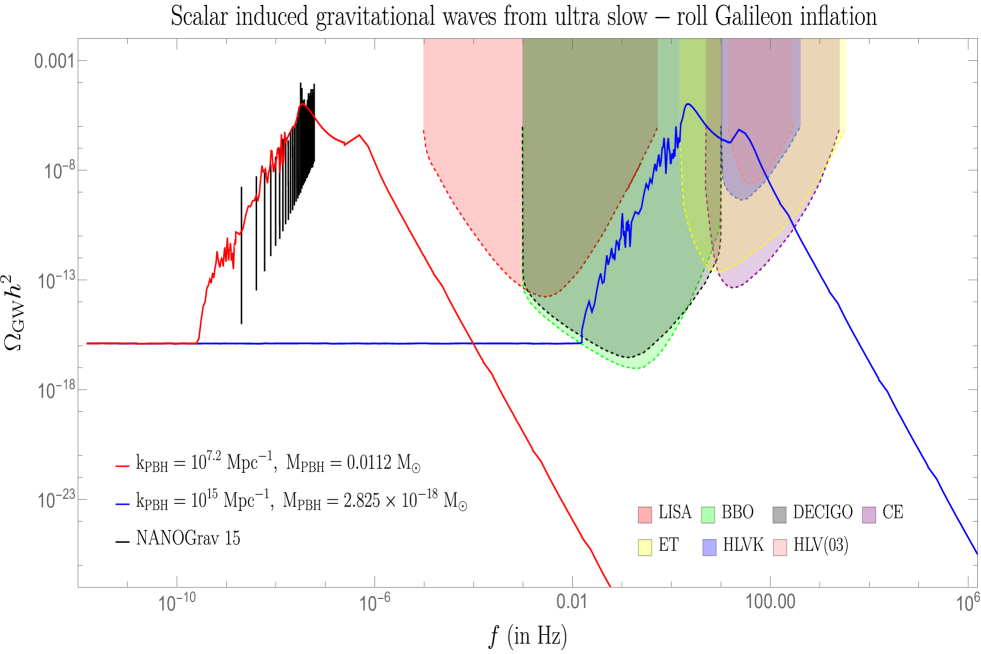
Figure 2: The plot represents the scalar-induced GW spectrum generated using the one-loop corrected version of the scalar power spectrum obtained in Galileon inflation. This figure contains $2$ separate features each distinguished by colors red and blue which indicate different scenarios. The red spectrum is where the amplitude of the generated signal coincides with the observational result from NANOGrav 15-year signal and it also indicates the production of $M_{\rm PBH}\sim 0.01M_{\odot}(2\times 10^{28}{\rm Kg})$ for a transition scale of $f_{\rm PBH}\sim 10^{-8}{\rm Hz}$. The blue spectrum is where the amplitude of the signal lies within the proposed sensitivity curves of the existing and future experiments to detect high-frequency GWs, which include the following: LISA, BBO, DECIGO, Cosmic Explorer(CE), Einstein Telescope(ET), HLVK network (consisting of detectors: aLIGO in Hanford and Livingstone, aVirgo, and KAGRA), and the HLV network during the third observation run (O3). This blue curve also shows a similar spectrum of GWs generated at a high-frequency value, near the transition scale $f_{\rm PBH}\sim 1{\rm Hz}$ where sub-solar PBH, $M_{\rm PBH}\sim 10^{-18}M_{\odot}(2\times 10^{2}{\rm Kg})$, are generated.

The values in range $(10^{-17}{\rm Hz},10^{-8}{\rm Hz})$ include part of the spectrum which contains information from the pivot scale $k_{*}\sim(10^{-2}{\rm Mpc}^{-1}\approx 10^{-17}{\rm Hz})$ up to the transition wavenumber $k_{\rm PBH}\sim 10^{7}{\rm Mpc}^{-1}(f_{\rm PBH}\sim 10^{-8}{\rm Hz})$. As we move higher in the frequency range from the frequency at the pivot scale, the spectrum shows a rise in amplitude, including small oscillations, which result from the highly oscillating integrand involved in the spectrum calculation. Up to a specific frequency, the behavior of the power spectrum changes, and we see that for a small region, the spectrum achieves a peak amplitude of $\Omega_{\rm GW}h^{2}\sim{\cal O}(10^{-5})$ which occurs as a result of the sharp transition encountered at the scale $k_{\rm PBH}$. After the peak, the amplitude of the spectrum starts to fall before going through a bump-like feature visible in the plot right after the frequency $f\sim 10^{-7}{\rm Hz}$. This feature is reminiscent of the similar effect observed in the one-loop corrected scalar power spectrum, fig.(1), for the comoving curvature perturbation, which occurs right after the transition at the wavenumber $k_{e}$ during the end of USR. Then, as we proceed towards completing the necessary e-foldings ${\cal N}=60$, the amplitude of the spectrum falls linearly and at a rate faster compared to its rise in the region before the peak, which results from the behavior of the scalar power spectrum in the frequency region corresponding to the SRII phase.

As we can see, the peak value of the GW spectrum shown in the plot coincides with the results observed in the NANOGrav 15-year Data Set. These observations show that inflation in Galileon theory has the required feature to produce the primordial GWs and nearly solar mass PBHs, $M_{\rm PBH}\sim 0.01M_{\odot}$.

The interesting feature to note in fig.(2) comes further when we shift the transition scale to higher wavenumbers where $k_{\rm PBH}\sim{\cal O}(10^{15}{\rm Mpc}^{-1}\approx 1{\rm Hz})$. There we observe a similar kind of behavior for the GW spectrum as was with the case when considering almost solar mass PBH, but this time, masses of the produced PBH are tiny, in the sub-solar regime $M_{\rm PBH}\sim 10^{-18}M_{\odot}$. For this case, the peak value of the GW spectrum falls into the sensitivity curves of the proposed and operational space and earth-based probes of GWs, which are in the background of the above figure for comparison. Maintaining the perturbativity approximation and benefits of the non-renormalization theorem has the GW spectrum preserve its behavior near the sharp transitions and have successful inflation after the end of the USR.

Hence, Galileon theory has the power to accommodate the possibility of producing PBHs within the sub-solar and solar mass range depending on the transition wavenumber $k_{\rm PBH}$ position and can produce enough amount of GW signal which can fall into the experimentally observed low-frequency regime from NANOGrav, as well as in the allowed sensitivity of the high-frequency regime probes.

V Conclusion

In this paper, we have considered the scalar-induced gravitational waves using the one-loop corrected scalar power spectrum from Galileon inflation. We first briefly reviewed the Galileon theory by introducing the action for the Covariantized Galileon Theory and then outlining the procedure to develop solutions for the comoving curvature perturbations modes in the three regions, SRI, USR, and SRII, by using the second-order action in this theory. The defining feature of this theory, other than the ability to evade the emergence of unwanted ghosts, is its non-renormalization theorem which allows us not to consider any renormalization and resummation procedure for the loop effects in its correlations. This feature helped us to manage a sufficient number of e-foldings of expansion and control the one-loop effects in theory, which later form part of the total scalar power spectrum necessary for further analysis regarding the GWs abundance calculation. We then presented a concise overview of the theory behind the scalar-induced gravitational waves (SIGWs) which tells us that the second-order tensor mode solutions involved quadratic contributions of the first-order scalar perturbations. After deriving the expression for the tensor power spectrum in terms of the scalar power spectrum, the next step was to numerically solve the integral for the GW abundance and plot the resulting behavior against the allowed frequency range. The features of this plot represent the key findings of our overall analysis done in this work.

We observed that the amount of GW abundance, $\Omega_{\rm GW}h^{2}$, produced through the use of one-loop corrected scalar power spectrum in the low-frequency region, $10^{-8}{\rm Hz}\leqslant f\leqslant 10^{-6}{\rm Hz}$, is such that it gives a sufficient overlap and thus indicates an agreement with the observational result from the NANOGrav 15-year signal. In the high-frequency region, after the peak value is achieved, the obtained spectrum falls rapidly compared to its ascent near the low-frequency values. The peak enhancement in the signal is due to a sharp transition feature when going from the SRI to USR phase. This behavior is known to exist for the total dimensionless scalar power spectrum in plot fig.(1) near the scales labeled as $k_{s}\sim 10^{6}{\rm Mpc}^{-1}$ and $k_{e}\sim 10^{7}{\rm Mpc}^{-1}$. There the property of accommodating a long enough SRII region required for successful inflation, $\Delta{\cal N}_{\rm Total}=60$, is also reflected in the tensor power spectrum, and equivalently the GW spectrum, when it is extended to even higher frequencies and their corresponding lower amplitudes relative to the current values.

The scale of the transition wave number determines the mass of the PBH being produced. Using the eqn.(18), we were able to find the allowed range of mass values, $(1M_{\odot}-10^{-18}M_{\odot})$, of the produced PBH when the transition scale is set between $k_{\rm PBH}\sim(10^{7}{\rm Mpc}^{-1}-10^{15}{\rm Mpc}^{-1})$. Hence, by keeping the transition scale near to the required value in the frequency range of the NANOGrav signal, $k_{\rm PBH}\sim(10^{7}{\rm Mpc}^{-1}\approx 10^{-8}{\rm Hz})$, we have shown that Galileon theory can produce almost solar mass PBH, $M_{\rm PBH}\sim 0.01M_{\odot}$, and along with that generate enough amount of observable signal in the GW spectrum. Next, we examined the case where the transition scale is pushed to the domain of higher frequencies where the existing and proposed GW experiments are able to probe the effect. We found that Galileon theory is also able to produce a sufficient amount of signal in the spectrum such that it falls under the parameter space of these experiments. The observed spectrum exactly mimics the behavior for the case of a transition scale in the lower frequencies. This is important from the perspective of future investigations regarding the observation of SIGWs in higher frequencies as a signal for new physics models. Due to the setting of the transition at such high wave numbers, $k_{\rm PBH}\sim(10^{15}{\rm Mpc}^{-1}\approx 1{\rm Hz})$, we are also able to predict the production of small mass PBHs in the sub-solar category, $M_{\rm PBH}\sim 10^{-18}M_{\odot}$, and also producing an observable amount of signal in the GW spectrum. This is again the result of the intrinsic properties of the Galileon theory, which does not depend on the scale of transition until we are able to satisfy the perturbativity criteria, which is maintained throughout our analysis by keeping $k_{e}/k_{s}\sim{\cal O}(10)$, where $k_{s},k_{e}$ are the respective scales at the SRI to USR and USR to SRII transitions. Thus, have demonstrated the possibility of generating a measurable spectrum of the GW abundance either in the low-frequency (NANOGrav) region or the high-frequency region of the ground- and space-based GW detectors and the production of corresponding masses of PBHs ranging from $(1M_{\odot}-10^{-18}M_{\odot})$.

VI Appendix

VI.1 General Mode Solutions

In this appendix, we focus on the calculation of the comoving curvature perturbations modes in the three phases SRI, USR, and SRII starting from setting up inflation within the CGT. The contents of this appendix is based on the detailed study provided in the refs.[125, 126].

Since we want to study the inflationary scenario on a quasi de-Sitter background, we require that a variation in the effective potential of our theory must satisfy the condition $|\Delta V/V|\ll 1$. This gives us a value of the scale factor within our CGT framework as $a(t)=\exp{(Ht)}$ where the Hubble parameter is used to define the slow-roll parameter $\epsilon=-\dot{H}/H^{2}$ describing deviation from exact de-Sitter.

Keeping these arguments in mind, we begin with the part of the action which is described using a background Galileon field $\bar{\phi}(t)$. Using integration by parts method and discarding the boundary terms leaves us with the action:

$$S^{(0)}=\int d^{4}x\,a^{3}\,\Bigg{\{}\dot{\bar{\phi}}^{2}\Bigg{(}\frac{c_{2}}{2}+2c_{3}Z+\frac{9c_{4}}{2}Z^{2}+6c_{5}Z^{3}\Bigg{)}+\lambda^{3}\bar{\phi}\Bigg{\}}$$ (47)

where the coupling parameter is defined as $Z\equiv H\dot{\bar{\phi}}/\Lambda^{3}$ with $\Lambda$ as a physical cut-off scale of the theory. In the regime where the coupling satisfies $Z\simeq 1$, we can incorporate the non-linearities within the galileon sector and also neglect any non-minimal couplings to gravity. This is the favourable regime in which we choose to work.

To study the perturbation theory at second order in the curvature perturbations, we require the need for a second order perturbed action. This action is written as follows in the Fourier space:

$$S^{(2)}_{\zeta}=\int d\tau\;\frac{d^{3}\mathbf{k}}{(2\pi)^{3}}a(\tau)^{2}\frac{\cal A}{H^{2}}\left(|\zeta_{\mathbf{k}}^{{}^{\prime}}(\tau)|^{2}-c_{s}^{2}k^{2}|\zeta_{\mathbf{k}}(\tau)|^{2}\right)=\int d\tau\;\frac{d^{3}\mathbf{k}}{(2\pi)^{3}}a(\tau)^{2}\frac{\cal B}{c_{s}^{2}H^{2}}\left(|\zeta_{\mathbf{k}}^{{}^{\prime}}(\tau)|^{2}-c_{s}^{2}k^{2}|\zeta_{\mathbf{k}}(\tau)|^{2}\right)$$ (48)

where ${\cal A}$ and ${\cal B}$ are coefficients depending on the conformal time, satisfying $c_{s}^{2}={\cal B}/{\cal A}$ for the speed of sound parameter in the CGT. Their explicit expressions are written down as follows:

$${\cal A} \equiv \frac{\dot{\bar{\phi}}^{2}}{2}\Bigg{(}c_{2}+12c_{3}Z+54c_{4}Z^{2}+120c_{5}Z^{3}\Bigg{)},$$ (49)

$${\cal B} \equiv \frac{\dot{\bar{\phi}}^{2}}{2}\Bigg{\{}c_{2}+4c_{3}\Bigg{(}2Z-\frac{H\dot{\bar{\phi}}}{\Lambda^{3}}\eta\Bigg{)}+2c_{4}\Bigg{[}13Z^{2}-\frac{6}{\Lambda^{6}}\dot{\bar{\phi}}^{2}H^{2}\big{(}\epsilon+2\eta\big{)}\Bigg{]}-\frac{24c_{5}}{\Lambda^{9}}H^{3}\dot{\bar{\phi}}^{3}\big{(}2\epsilon+1\big{)}\Bigg{\}}.$$ (50)

which also includes the second slow-roll parameter $\eta$. Solving of the above second order action would give us the following solution:

$$\zeta^{{}^{\prime\prime}}_{\bf k}(\tau)+2\frac{z^{{}^{\prime}}(\tau)}{z(\tau)}\zeta^{{}^{\prime}}_{\bf k}(\tau)+c^{2}_{s}k^{2}\zeta_{\mathbf{k}}(\tau)=0.$$ (51)

with $z(\tau)=a\sqrt{2{\cal A}}/H^{2}$. It is this equation whose solutions in the three phases are to be analyzed. This is performed by the setting of the initial conditions for the SRI phase as the Bunch-Davies quantum vacuum state and in the subsequent phases we are required to solve the boundary conditions during the transitions to eventually determine their complete solutions. We now describe the mode solutions for each phase.

• For the SRI phase:
  The general mode solution in this phase for the second-order Fourier space equation of motion turns out to be:

  $$\zeta_{\mathbf{k}}(\tau) = \left(\frac{iH^{2}}{2\sqrt{\cal A}}\right)\frac{1}{(c_{s}k)^{3/2}}\times\left[\alpha^{(1)}_{\mathbf{k}}\left(1+ikc_{s}\tau\right)\exp{\left(-ikc_{s}\tau\right)}-\beta^{(1)}_{\mathbf{k}}\left(1-ikc_{s}\tau\right)\exp{\left(ikc_{s}\tau\right)}\right]$$ (52)

  where the conformal time window is the interval with $\tau<\tau_{s}$. The Bogoliubov coefficients for this phase are obtained as the result of fixing the Bunch-Davies initial condition:

  $$\alpha^{(1)}_{\bf k}=1,$$ (53)

  $$\beta^{(1)}_{\bf k}=0.$$ (54)

  Throughout this phase, the slow-roll parameter $\epsilon(\tau)$ is almost a constant while for the other slow-roll parameter $\eta(\tau)\sim 0$.

• For the USR phase:
  The general mode solution in this phase, for the conformal time window $\tau\in\left[\tau_{s},\tau_{e}\right)$, is obtained to be as follows:

  $$\zeta_{\mathbf{k}}(\tau) = \left(\frac{iH^{2}}{2\sqrt{\cal A}}\right)\left(\frac{\tau_{s}}{\tau}\right)^{3}\frac{1}{(c_{s}k)^{3/2}}\times\left[\alpha^{(2)}_{\bf k}\left(1+ikc_{s}\tau\right)\exp{\left(-ikc_{s}\tau\right)}-\beta^{(2)}_{\bf k}\left(1-ikc_{s}\tau\right)\exp{\left(ikc_{s}\tau\right)}\right].$$ (55)

  The parameter $\epsilon$ behaves very differently for this phase with having a time-dependent form: $\epsilon(\tau)=\epsilon(\tau/\tau_{s})^{6}$. This effect is reflected in the above equation. To have the complete solution requires the solving of the continuity and differentiability conditions at the transition scale $\tau_{s}$. As a result, we obtain the following Bogoliubov coefficients:

  $$\alpha^{(2)}_{\bf k} = 1+\frac{3k_{s}^{3}}{2ik^{3}}\left(1+\left(\frac{k}{k_{s}}\right)^{2}\right),$$ (56)

  $$\beta^{(2)}_{\bf k} = \frac{3k_{s}^{3}}{2ik^{3}}\left(1-i\left(\frac{k}{k_{s}}\right)^{2}\right)^{2}\;\exp{\left(2i\frac{k}{k_{s}}\right)}.$$ (57)

  However, the parameter $\eta(\tau)$ here satisfies $\eta\sim-6$ which indicates an extreme jump from the previous value and is the cause for the enhancement in the fluctuations.

• For the SRII phase:
  The general mode solution in this phase, for the conformal time window $\tau\in\left[\tau_{e},\tau_{{\rm end}}\right]$, is obtained to be as follows:

  $$\zeta_{\mathbf{k}}(\tau) = \left(\frac{iH^{2}}{2\sqrt{\cal A}}\right)\left(\frac{\tau_{s}}{\tau_{e}}\right)^{3}\frac{1}{(c_{s}k)^{3/2}}\times\left[\alpha^{(3)}_{\bf k}\left(1+ikc_{s}\tau\right)\exp{\left(-ikc_{s}\tau\right)}-\beta^{(3)}_{\bf k}\left(1-ikc_{s}\tau\right)\exp{\left(ikc_{s}\tau\right)}\right].$$ (58)

  The parameter $\epsilon$ in this phase has the behaviour where it varies slowly as a result of its form:$\epsilon(\tau)=\epsilon(\tau_{e}/\tau_{s})$. This fact is crucial for the above solution. Again, through the use of the boundary conditions we get the following form of the Bogoliubov coefficients in this phase:

  $$\alpha^{(3)}_{\bf k} = -\frac{k_{s}^{3}k_{e}^{3}}{4k^{6}}\Bigg{[}9\left(-\frac{k}{k_{e}}+i\right){}^{2}\left(\frac{k}{k_{s}}+i\right){}^{2}\exp{\left(2ik\left(\frac{1}{k_{s}}-\frac{1}{k_{e}}\right)\right)}$$ (59)

  $$\quad\quad\quad\quad\quad\quad\quad\quad\quad\quad\quad\quad\quad\quad-\left\{\left(\frac{k}{k_{e}}\right)^{2}\left(-2\frac{k}{k_{e}}-3i\right)-3i\right\}\left\{\left(\frac{k}{k_{s}}\right)^{2}\left(-2\frac{k}{k_{s}}+3i\right)+3i\right\}\Bigg{]},$$

  $$\beta^{(3)}_{\bf k} = \frac{3k_{s}^{3}k_{e}^{3}}{4k^{6}}\Bigg{[}\left(\frac{k}{k_{s}}+i\right)^{2}\left\{\left(\frac{k}{k_{e}}\right)^{2}\left(2i\frac{k}{k_{e}}\right)+3\right\}\exp{\left(2i\frac{k}{k_{s}}\right)}$$ (60)

  $$\quad\quad\quad\quad\quad\quad\quad\quad\quad\quad\quad\quad\quad\quad\quad\quad+i\left(\frac{k}{k_{e}}+i\right)^{2}\left\{3i+\left(\frac{k}{k_{s}}\right)^{2}\left(-2\frac{k}{k_{s}}+3i\right)\right\}\exp{\left(2i\frac{k}{k_{e}}\right)}\Bigg{]}.$$

  For this phase, the parameter $\eta(\tau)$ has an almost constant value throughout. This is quite similar to the behavior of the same parameter in the SRI phase. This nature is also reflected in the final behaviour of the power spectrum during this phase.

In all the equations above we have used the horizon crossing condition $-kc_{s}\tau=1$ which is valid in all three phases during the sharp transitions at $k_{s}$ from the SRI to USR phase and at $k_{e}$ for the USR to SRII phase. These equations are sufficient to write the tree-level scalar power spectrum in the super-horizon limit, which we now mention as:

$$\Delta^{2}_{\zeta,{\bf Tree}}(k) = \displaystyle\displaystyle\left(\frac{H^{4}}{8\pi^{2}{\cal A}c^{3}_{s}}\right)_{*}\times\left\{\begin{array}[]{ll}\displaystyle 1+\Bigg{(}\frac{k}{k_{s}}\Bigg{)}^{2}&\mbox{when}\quad k<k_{s}\;(\rm SRI)\\ \displaystyle\displaystyle\left(\frac{k_{e}}{k_{s}}\right)^{6}\left|\alpha^{(2)}_{\bf k}-\beta^{(2)}_{\bf k}\right|^{2}&\mbox{when }k_{s}\leqslant k<k_{e}\;(\rm USR)\\ \displaystyle\displaystyle\left(\frac{k_{e}}{k_{s}}\right)^{6}\left|\alpha^{(3)}_{\bf k}-\beta^{(3)}_{\bf k}\right|^{2}&\mbox{when }k_{e}\leqslant k\leqslant k_{\rm end}\;(\rm SRII)\end{array}\right.$$ (64)

VI.2 Couplings and Coefficients in three phases including one-loop effects

In this appendix, we present the expressions for the couplings and the momentum-dependent functions which are necessary to describe the one-loop contributions to the total scalar power spectrum.

• For the SRI phase: The one-loop effect from the SRI phase which contributes into the total scalar power spectrum is written as follows:

  $$\Bigg{[}\Delta^{2}_{\zeta,\bf{One-Loop}}(k)\Bigg{]}_{\rm\textbf{SRI}}=\Bigg{[}\Delta^{2}_{\zeta,\bf{Tree}}(k)\Bigg{]}_{\rm\textbf{SRI}}\times\left(-\sum^{4}_{i=1}{\cal G}_{i,\mathbf{SRI}}\mathbf{F}_{i,\mathbf{SRI}}(k_{s},k_{*})\right)$$ (65)

  the values for ${\cal G}_{i,\textbf{SRI}}\;\forall i=1,2,3,4$ are defined using the CGT couplings:

  $${\cal G}_{1,{\bf SRI}} = {\cal G}^{2}_{1}(\tau_{*})$$

  $${\cal G}_{2,{\bf SRI}} = -{\cal G}^{2}_{2}(\tau_{*})H^{2}(\tau_{*})c^{2}_{s}$$

  $${\cal G}_{3,{\bf SRI}} = -\frac{{\cal G}^{2}_{3}(\tau_{*})}{c^{2}_{s}}$$

  $${\cal G}_{4,{\bf SRI}} = \frac{{\cal G}^{2}_{4}(\tau_{*})H^{2}(\tau_{*})}{c^{6}_{s}}$$

  and the momentum-dependent functions $\mathbf{F}_{i,\textbf{SRI}}$ are defined using the notation ${\cal K}_{*,s}\equiv k_{*}/k_{s}$ as follows:

  $${\bf F}_{1,{\bf SRI}}(k_{s},k_{*}) = \frac{1}{2}\Bigg{[}3+{\cal K}_{*,s}^{2}\Bigg{]},$$ (67)

  $${\bf F}_{2,{\bf SRI}}(k_{s},k_{*}) = \Bigg{[}\frac{17}{42}-\frac{2}{3}{\cal K}_{*,s}^{6}+\frac{24}{7}{\cal K}_{*,s}^{7}-\frac{9}{2}{\cal K}_{*,s}^{8}\Bigg{]},$$ (68)

  $${\bf F}_{3,{\bf SRI}}(k_{s},k_{*}) = -\frac{2}{3}\Bigg{[}1-{\cal K}_{*,s}^{6}\Bigg{]},$$ (69)

  $${\bf F}_{4,{\bf SRI}}(k_{s},k_{*}) = -\frac{1}{2}\Bigg{[}1-{\cal K}_{*,s}^{2}\Bigg{]}.$$ (70)

• For the USR phase: The one-loop effect from the USR phase which contributes into the total scalar power spectrum is written as follows:

  $$\Bigg{[}\Delta^{2}_{\zeta,\bf{One-Loop}}(k)\Bigg{]}_{\rm\textbf{USR}}=\Bigg{[}\Delta^{2}_{\zeta,\bf{Tree}}(k)\Bigg{]}_{\rm\textbf{SRI}}\times\left(\sum^{4}_{i=1}{\cal G}_{i,\mathbf{USR}}\mathbf{F}_{i,\mathbf{SRI}}(k_{e},k_{s})\right)$$ (71)

  the values for ${\cal G}_{i,\textbf{USR}}\;\forall i=1,2,3,4$ are defined using the CGT couplings:

  $${\cal G}_{1,{\bf USR}} = \Bigg{(}\frac{{\cal G}^{2}_{1}(\tau_{e})}{c^{3}_{s}}{\cal K}_{e,s}^{6}-\frac{{\cal G}^{2}_{1}(\tau_{s})}{c^{3}_{s}}\Bigg{)}$$

  $${\cal G}_{2,{\bf USR}} = \Bigg{(}\frac{{\cal G}^{2}_{2}(\tau_{e})H^{2}(\tau_{e})}{c^{5}_{s}}{\cal K}_{e,s}^{4}-\frac{{\cal G}^{2}_{2}(\tau_{s})H^{2}(\tau_{s})}{c^{5}_{s}}\Bigg{)}$$

  $${\cal G}_{3,{\bf USR}} = \Bigg{(}\frac{{\cal G}^{2}_{3}(\tau_{e})}{c^{6}_{s}}{\cal K}_{e,s}^{3}-\frac{{\cal G}^{2}_{3}(\tau_{s})}{c^{6}_{s}}\Bigg{)}$$

  $${\cal G}_{4,{\bf USR}} = \Bigg{(}\frac{{\cal G}^{2}_{2}(\tau_{e})H^{2}(\tau_{e})}{c^{7}_{s}}{\cal K}_{e,s}^{2}-\frac{{\cal G}^{2}_{2}(\tau_{s})H^{2}(\tau_{s})}{c^{7}_{s}}\Bigg{)}.$$

  where we have used the notation ${\cal K}_{e,s}\equiv k_{e}/k_{s},\;\text{and}\;{\cal K}_{s,e}\equiv k_{s}/k_{e}$. Using these same notations further we write the momentum-dependent functions $\mathbf{F}_{i,\textbf{USR}}$ as follows:

  $${\bf F}_{1,{\bf USR}}(k_{e},k_{s}) = \Bigg{[}\frac{1}{4}+\frac{9}{4}{\cal K}_{s,e}^{2}-\frac{1}{4}{\cal K}_{s,e}^{4}-9{\cal K}_{s,e}^{4}\ln{\cal K}_{s,e}-6\sin\left(1+{\cal K}_{e,s}\right)\sin\left(1-{\cal K}_{e,s}\right)$$ (73)

  $$\quad-\frac{9}{8}{\cal K}_{s,e}^{2}\Bigg{\{}2\left(\frac{k_{e}}{k_{s}}\right)\sin\left(2{\cal K}_{e,s}\right)-\cos\left(2{\cal K}_{e,s}\right)\Bigg{\}}-6{\cal K}_{s,e}\sin\left(2{\cal K}_{e,s}\right)$$

  $$\quad-\frac{69}{16}\cos\left(2{\cal K}_{e,s}\right)-\frac{3}{4}{\cal K}_{s,e}^{2}\Bigg{\{}2{\cal K}_{e,s}\cos\left(2{\cal K}_{e,s}\right)-\sin\left(2{\cal K}_{e,s}\right)\Bigg{\}}\Bigg{]},$$

  $${\bf F}_{2,{\bf USR}}(k_{e},k_{s}) = \Bigg{[}\frac{1}{8}+\frac{9}{12}{\cal K}_{s,e}^{2}+\frac{9}{4}{\cal K}_{s,e}^{4}+\frac{9}{4}{\cal K}_{s,e}^{6}-\frac{43}{8}{\cal K}_{s,e}^{8}-\frac{9}{8}\cos\left(2{\cal K}_{e,s}\right)\Bigg{]},$$ (74)

  $${\bf F}_{3,{\bf USR}}(k_{e},k_{s}) = \Bigg{[}\frac{1}{8}+\frac{9}{12}{\cal K}_{s,e}^{2}+\frac{9}{4}{\cal K}_{s,e}^{4}+\frac{9}{4}{\cal K}_{s,e}^{6}-\frac{43}{8}{\cal K}_{s,e}^{8}-\frac{9}{8}\cos\left(2{\cal K}_{e,s}\right)\Bigg{]}$$ (75)

  $$= {\bf F}_{2,{\bf USR}}(k_{e},k_{s}),$$

  $${\bf F}_{4,{\bf USR}}(k_{e},k_{s}) = \Bigg{[}\frac{1}{12}+\frac{9}{20}{\cal K}_{s,e}^{2}+\frac{9}{8}{\cal K}_{s,e}^{4}+\frac{9}{12}{\cal K}_{s,e}^{6}-\frac{299}{230}{\cal K}_{s,e}^{12}\Bigg{]}.$$ (76)

• For the SRII phase: The one-loop effect from the SRII phase which contributes into the total scalar power spectrum is written as follows:

  $$\Bigg{[}\Delta^{2}_{\zeta,\bf{One-Loop}}(k)\Bigg{]}_{\rm\textbf{SRII}}=\Bigg{[}\Delta^{2}_{\zeta,\bf{Tree}}(k)\Bigg{]}_{\rm\textbf{SRI}}\times\left(\sum^{4}_{i=1}{\cal G}_{i,\mathbf{SRII}}\mathbf{F}_{i,\mathbf{SRII}}(k_{\rm end},k_{e})\right)$$ (77)

  the values for ${\cal G}_{i,\textbf{SRII}}\;\forall i=1,2,3,4$ are defined using the CGT couplings:

  $${\cal G}_{1,{\bf SRII}} = \Bigg{(}\frac{{\cal G}^{2}_{1}(\tau_{\rm end})}{c^{3}_{s}}{\cal K}_{e,s}^{6}-\frac{{\cal G}^{2}_{1}(\tau_{e})}{c^{3}_{s}}\Bigg{)}$$

  $${\cal G}_{2,{\bf SRII}} = \Bigg{(}\frac{{\cal G}^{2}_{2}(\tau_{\rm end})H^{2}(\tau_{\rm end})}{c^{5}_{s}}{\cal K}_{e,s}^{4}-\frac{{\cal G}^{2}_{2}(\tau_{e})H^{2}(\tau_{e})}{c^{5}_{s}}\Bigg{)}$$

  $${\cal G}_{3,{\bf SRII}} = \Bigg{(}\frac{{\cal G}^{2}_{3}(\tau_{\rm end})}{c^{6}_{s}}{\cal K}_{e,s}^{3}-\frac{{\cal G}^{2}_{3}(\tau_{e})}{c^{6}_{s}}\Bigg{)}$$

  $${\cal G}_{4,{\bf SRII}} = \Bigg{(}\frac{{\cal G}^{2}_{2}(\tau_{\rm end})H^{2}(\tau_{\rm end})}{c^{7}_{s}}{\cal K}_{e,s}^{2}-\frac{{\cal G}^{2}_{2}(\tau_{e})H^{2}(\tau_{e})}{c^{7}_{s}}\Bigg{)}$$

  where ${\cal K}_{e,s}\;\text{and}\;{\cal K}_{s,e}$ are previously defined in the USR phase. The momentum-dependent functions $\mathbf{F}_{i,\textbf{SRII}}$ are defined here after taking out only the leading order contributions and $"\cdots"$ are used to represent the suppressed quantities. To write the expressions more concisely, we choose the following notation:

  $${\cal K}_{{\rm end},e}\equiv\frac{k_{\rm end}}{k_{e}},\quad\quad{\cal K}_{{\rm end},s}\equiv\frac{k_{\rm end}}{k_{s}},\quad\quad{\cal K}_{e,{\rm end}}\equiv\frac{k_{e}}{k_{\rm end}},\quad\quad{\cal K}_{s,{\rm end}}\equiv\frac{k_{s}}{k_{\rm end}}$$ (79)

  The final result is written as follows:

$${\bf F}_{1,{\bf SRII}}(k_{\rm end},k_{e}) = \Bigg{[}\frac{81}{64}+\frac{81}{40}\left(1+{\cal K}_{s,e}\right)-\frac{9}{8}\left(1+{\cal K}_{s,e}^{2}\right)+\frac{1}{6}\left(\left(1+{\cal K}_{s,e}\right)^{2}+2{\cal K}_{s,e}\right)+\frac{1}{8}{\cal K}_{s,e}^{2}+6+\frac{2}{7}{\cal K}_{s,e}\left(1+{\cal K}_{s,e}\right)$$ (80)

$$+\frac{27}{8}\left(1+{\cal K}_{s,e}^{6}\right)-\frac{3}{4}{\cal K}_{e,{\rm end}}\cos\left(2{\cal K}_{{\rm end},e}\right)+4{\cal K}_{e,{\rm end}}^{2}\ln\left({\cal K}_{e,{\rm end}}\right)-\frac{3}{4}\sin\left(1+{\cal K}_{{\rm end},s}\right)\sin\left(1-{\cal K}_{{\rm end},s}\right)$$

$$-\frac{9}{4}\frac{\displaystyle{\cal K}_{s,e}}{\displaystyle\left(1-{\cal K}_{s,e}\right)^{2}}\Bigg{\{}\cos\left(2\left({\cal K}_{{\rm end},e}-{\cal K}_{{\rm end},s}\right)\right)\Bigg{\}}-\frac{9}{4}\frac{\displaystyle 1}{\displaystyle\left(1-{\cal K}_{s,e}\right)}\Bigg{\{}{\cal K}_{s,{\rm end}}\sin\left(2\left({\cal K}_{{\rm end},e}-{\cal K}_{{\rm end},s}\right)\right)\Bigg{\}}$$

$$-9\frac{\displaystyle\left(1+{\cal K}_{s,e}\right)^{2}}{\displaystyle\left(1-{\cal K}_{s,e}\right)}\Bigg{\{}\sin\left(2\left({\cal K}_{{\rm end},e}-{\cal K}_{{\rm end},s}\right)\right)\Bigg{\}}+\frac{9}{8}\Bigg{\{}8-18{\cal K}_{s,e}^{4}\left(1+{\cal K}_{s,e}\right)\Bigg{\}}$$

$$\Bigg{\{}\cos\left(2\left({\cal K}_{{\rm end},e}-{\cal K}_{{\rm end},s}\right)\right)-{\cal K}_{e,{\rm end}}\cos\left(2\left(1-{\cal K}_{e,s}\right)\right)\Bigg{\}}-\frac{9}{16}{\cal K}_{s,e}^{2}\left(9+44{\cal K}^{2}_{s,e}\right)\ln{\cal K}_{e,{\rm end}}$$

$$+9{\cal K}_{s,e}^{4}\left(1+{\cal K}_{s,e}^{2}\right)+\frac{9}{7}{\cal K}_{s,e}^{6}+22{\cal K}_{s,e}^{2}\left(1-{\cal K}_{e,{\rm end}}\right)$$

$$-\frac{27}{16}{\cal K}_{s,e}^{4}{\cal K}_{e,{\rm end}}\Bigg{\{}\sin\left(2{\cal K}_{{\rm end},e}\right)-{\cal K}_{e,{\rm end}}\cos\left(2{\cal K}_{{\rm end},e}\right)\Bigg{\}}\cdots\Bigg{]},$$

$${\bf F}_{2,{\bf SRII}}(k_{\rm end},k_{e}) = \Bigg{[}\frac{81}{16}\ln{\cal K}_{e,{\rm end}}+\frac{81}{8}\left(1-{\cal K}_{e,{\rm end}}\right)\left(1+{\cal K}_{s,e}\right)+5{\cal K}_{s,e}^{6}\ln{\cal K}_{e,{\rm end}}$$ (81)

$$+\frac{1}{2}\left(\left(1+{\cal K}_{s,e}\right)^{2}+2{\cal K}_{s,e}\right)+\frac{2}{3}\left(1-{\cal K}_{e,{\rm end}}^{3}\right){\cal K}_{s,e}\left(1+{\cal K}_{s,e}\right)+\frac{1}{4}{\cal K}_{s,e}^{2}+\frac{1}{4}+\frac{27}{64}-\frac{27}{8}\left(1+{\cal K}_{s,e}^{6}\right)$$

$$+\frac{3}{8}\left(1+{\cal K}_{s,e}^{2}\right)-\frac{9}{16}\frac{\displaystyle{\cal K}_{s,e}^{3}}{\displaystyle\left(1-{\cal K}_{s,e}\right)^{2}}\Bigg{\{}\cos\left(2\left({\cal K}_{{\rm end},e}-{\cal K}_{{\rm end},s}\right)\right)\Bigg{\}}$$

$$-\frac{27}{4}\frac{\displaystyle 1}{\displaystyle\left(1-{\cal K}_{s,e}\right)}\Bigg{\{}{\cal K}_{s,{\rm end}}\sin\left(2\left({\cal K}_{{\rm end},e}-{\cal K}_{{\rm end},s}\right)\right)\Bigg{\}}+\frac{81}{16}\frac{\displaystyle\left(1+{\cal K}_{s,e}^{2}\right)}{\displaystyle\left(1-{\cal K}_{s,e}\right)}\Bigg{\{}\cos\left(2\left({\cal K}_{{\rm end},e}-{\cal K}_{{\rm end},s}\right)\right)\Bigg{\}}$$

$$-\frac{9}{16}\frac{\displaystyle{\cal K}_{s,e}^{3}}{\displaystyle\left(1-{\cal K}_{s,e}\right)}\Bigg{\{}\sin\left(2\left({\cal K}_{{\rm end},e}-{\cal K}_{{\rm end},s}\right)\right)\Bigg{\}}-\frac{9}{16}\left(1+\left(\frac{k_{e}}{k_{s}}\right)\right)\Bigg{\{}{\cal K}_{e,{\rm end}}\cos\left(2\left({\cal K}_{{\rm end},e}-{\cal K}_{{\rm end},s}\right)\right)\Bigg{\}}$$

$$+\frac{27}{16}{\cal K}_{s,e}^{6}+\frac{81}{64}{\cal K}_{s,e}^{6}-\frac{9}{32}{\cal K}_{s,e}^{2}\left(9+8{\cal K}_{s,e}^{2}+36{\cal K}_{s,e}^{4}\right)\left(1-{\cal K}_{e,{\rm end}}\right)-\frac{81}{16}{\cal K}_{s,e}^{4}\left(1+{\cal K}_{s,e}^{2}\right)$$

$$+\left(1+4{\cal K}_{s,e}^{2}+{\cal K}_{s,e}^{4}\right)\ln{\cal K}_{e,{\rm end}}-\frac{3}{4}{\cal K}_{e,{\rm end}}\cos\left(2{\cal K}_{{\rm end},e}\right)\cdots\Bigg{]}={\bf F}_{3,{\bf SRII}}(k_{\rm end},k_{e}),$$

$${\bf F}_{4,{\bf SRII}}(k_{\rm end},k_{e}) = \Bigg{[}\frac{81}{16}+\frac{27}{8}\left(1+{\cal K}_{s,e}\right)+\frac{81}{16}{\cal K}_{s,e}^{6}\ln{\cal K}_{e,{\rm end}}+\frac{81}{32}\left(\left(1+{\cal K}_{s,e}\right)^{2}+2{\cal K}_{s,e}\right)$$ (82)

$$+10{\cal K}_{s,e}\left(1+{\cal K}_{s,e}\right)+\frac{1}{12}+\frac{9}{40}\left(1+{\cal K}_{s,e}^{2}\right)+\frac{27}{64}\left(1+{\cal K}_{s,e}^{6}\right)+\frac{81}{128}+6{\cal K}_{s,e}^{2}\ln{\cal K}_{e,{\rm end}}$$

$$-\frac{9}{16}\frac{\displaystyle\left(1+{\cal K}_{s,e}\right)^{2}}{\displaystyle\left(1-{\cal K}_{s,e}\right)^{2}}\Bigg{\{}\cos\left(2\left({\cal K}_{{\rm end},e}-{\cal K}_{{\rm end},s}\right)\right)\Bigg{\}}-\frac{27}{8}\frac{\displaystyle\displaystyle\left(1+{\cal K}_{s,e}\right)^{2}}{\displaystyle\left(1-{\cal K}_{s,e}\right)^{3}}\Bigg{\{}\sin\left(2\left({\cal K}_{{\rm end},e}-{\cal K}_{{\rm end},s}\right)\right)\Bigg{\}}$$

$$-\frac{27}{4}\frac{\displaystyle\displaystyle\left(1+{\cal K}_{s,e}\right)^{2}}{\displaystyle\left(1-{\cal K}_{s,e}\right)}\Bigg{\{}{\cal K}_{e,{\rm end}}^{2}\sin\left(2\left({\cal K}_{{\rm end},e}-{\cal K}_{{\rm end},s}\right)\right)\Bigg{\}}+\frac{9}{80}{\cal K}_{s,e}^{2}\left(9+44{\cal K}_{s,e}^{2}\right)+\frac{27}{8}{\cal K}_{s,e}^{4}\left(1+{\cal K}_{s,e}^{2}\right)$$

$$+\frac{81}{16}{\cal K}_{s,e}^{6}\left(1-{\cal K}_{e,{\rm end}}\right)+\frac{99}{56}+\frac{1}{4}{\cal K}_{e,{\rm end}}^{2}+\frac{81}{32}{\cal K}_{s,e}^{6}{\cal K}_{e,{\rm end}}\Bigg{\{}\sin\left(2{\cal K}_{{\rm end},e}\right)-{\cal K}_{e,{\rm end}}\cos\left(2{\cal K}_{{\rm end},e}\right)\Bigg{\}}\cdots\Bigg{]}.\quad\quad\quad$$

In terms of the above equations defined for all the three phases, the one-loop corrections to the scalar power spectrum from each of these phases can be written using the following expression:

$$\Delta^{2}_{\zeta,{\bf One-Loop}}(k) = \displaystyle\displaystyle\Bigg{[}\Delta^{2}_{\zeta,\bf{Tree}}(k)\Bigg{]}_{\rm\textbf{SRI}}\times\left\{\begin{array}[]{ll}\displaystyle-\sum^{4}_{i=1}{\cal G}_{i,\mathbf{SRI}}\mathbf{F}_{i,\mathbf{SRI}}(k_{s},k_{*})&\mbox{when}\quad k<k_{s}\;(\rm SRI)\\ \displaystyle\displaystyle\sum^{4}_{i=1}{\cal G}_{i,\mathbf{USR}}\mathbf{F}_{i,\mathbf{USR}}(k_{e},k_{s})\;\Theta(k-k_{s})&\mbox{when }k_{s}\leqslant k<k_{e}\;(\rm USR)\\ \displaystyle\displaystyle\sum^{4}_{i=1}{\cal G}_{i,\mathbf{SRII}}\mathbf{F}_{i,\mathbf{SRII}}(k_{\rm end},k_{e})\;\Theta(k-k_{e})&\mbox{when }k_{e}\leqslant k\leqslant k_{\rm end}\;(\rm SRII)\end{array}\right.$$ (86)

Combining Eqs.(64, 86) gives us the total dimensionless one-loop corrected version of the primordial scalar power spectrum which we ultimately utilize to generate the scalar-induced GW spectrum in Galileon inflation.

References

- [1] LIGO Scientific, Virgo Collaboration, B. P. Abbott et al., “Observation of Gravitational Waves from a Binary Black Hole Merger,” Phys. Rev. Lett. 116 no. 6, (2016) 061102, arXiv:1602.03837 [gr-qc].
- [2] L. Zu, C. Zhang, Y.-Y. Li, Y.-C. Gu, Y.-L. S. Tsai, and Y.-Z. Fan, “Mirror QCD phase transition as the origin of the nanohertz Stochastic Gravitational-Wave Background,” arXiv:2306.16769 [astro-ph.HE].
- [3] K. T. Abe and Y. Tada, “Translating nano-Hertz gravitational wave background into primordial perturbations taking account of the cosmological QCD phase transition,” arXiv:2307.01653 [astro-ph.CO].
- [4] Y. Gouttenoire, “First-order Phase Transition interpretation of PTA signal produces solar-mass Black Holes,” arXiv:2307.04239 [hep-ph].
- [5] NANOGrav Collaboration, Z. Arzoumanian et al., “Searching for Gravitational Waves from Cosmological Phase Transitions with the NANOGrav 12.5-Year Dataset,” Phys. Rev. Lett. 127 no. 25, (2021) 251302, arXiv:2104.13930 [astro-ph.CO].
- [6] X. Xue et al., “Constraining Cosmological Phase Transitions with the Parkes Pulsar Timing Array,” Phys. Rev. Lett. 127 no. 25, (2021) 251303, arXiv:2110.03096 [astro-ph.CO].
- [7] Y. Nakai, M. Suzuki, F. Takahashi, and M. Yamada, “Gravitational Waves and Dark Radiation from Dark Phase Transition: Connecting NANOGrav Pulsar Timing Data and Hubble Tension,” Phys. Lett. B 816 (2021) 136238, arXiv:2009.09754 [astro-ph.CO].
- [8] P. Athron, A. Fowlie, C.-T. Lu, L. Morris, L. Wu, Y. Wu, and Z. Xu, “Can supercooled phase transitions explain the gravitational wave background observed by pulsar timing arrays?,” arXiv:2306.17239 [hep-ph].
- [9] E. Madge, E. Morgante, C. Puchades-Ibáñez, N. Ramberg, W. Ratzinger, S. Schenk, and P. Schwaller, “Primordial gravitational waves in the nano-Hertz regime and PTA data – towards solving the GW inverse problem,” arXiv:2306.14856 [hep-ph].
- [10] N. Kitajima, J. Lee, K. Murai, F. Takahashi, and W. Yin, “Nanohertz Gravitational Waves from Axion Domain Walls Coupled to QCD,” arXiv:2306.17146 [hep-ph].
- [11] E. Babichev, D. Gorbunov, S. Ramazanov, R. Samanta, and A. Vikman, “NANOGrav spectral index from melting domain walls,” arXiv:2307.04582 [hep-ph].
- [12] Z. Zhang, C. Cai, Y.-H. Su, S. Wang, Z.-H. Yu, and H.-H. Zhang, “Nano-Hertz gravitational waves from collapsing domain walls associated with freeze-in dark matter in light of pulsar timing array observations,” arXiv:2307.11495 [hep-ph].
- [13] Z.-M. Zeng, J. Liu, and Z.-K. Guo, “Enhanced curvature perturbations from spherical domain walls nucleated during inflation,” arXiv:2301.07230 [astro-ph.CO].
- [14] R. Z. Ferreira, A. Notari, O. Pujolas, and F. Rompineve, “Gravitational waves from domain walls in Pulsar Timing Array datasets,” JCAP 02 (2023) 001, arXiv:2204.04228 [astro-ph.CO].
- [15] H. An and C. Yang, “Gravitational Waves Produced by Domain Walls During Inflation,” arXiv:2304.02361 [hep-ph].
- [16] X.-F. Li, “Probing the high temperature symmetry breaking with gravitational waves from domain walls,” arXiv:2307.03163 [hep-ph].
- [17] J. Ellis and M. Lewicki, “Cosmic String Interpretation of NANOGrav Pulsar Timing Data,” Phys. Rev. Lett. 126 no. 4, (2021) 041304, arXiv:2009.06555 [astro-ph.CO].
- [18] S. Blasi, V. Brdar, and K. Schmitz, “Has NANOGrav found first evidence for cosmic strings?,” Phys. Rev. Lett. 126 no. 4, (2021) 041305, arXiv:2009.06607 [astro-ph.CO].
- [19] W. Buchmuller, V. Domcke, and K. Schmitz, “From NANOGrav to LIGO with metastable cosmic strings,” Phys. Lett. B 811 (2020) 135914, arXiv:2009.10649 [astro-ph.CO].
- [20] J. J. Blanco-Pillado, K. D. Olum, and J. M. Wachter, “Comparison of cosmic string and superstring models to NANOGrav 12.5-year results,” Phys. Rev. D 103 no. 10, (2021) 103512, arXiv:2102.08194 [astro-ph.CO].
- [21] W. Buchmuller, V. Domcke, and K. Schmitz, “Stochastic gravitational-wave background from metastable cosmic strings,” JCAP 12 no. 12, (2021) 006, arXiv:2107.04578 [hep-ph].
- [22] K. Inomata, K. Kohri, and T. Terada, “The Detected Stochastic Gravitational Waves and Subsolar-Mass Primordial Black Holes,” arXiv:2306.17834 [astro-ph.CO].
- [23] Q.-H. Zhu, Z.-C. Zhao, and S. Wang, “Joint implications of BBN, CMB, and PTA Datasets for Scalar-Induced Gravitational Waves of Second and Third orders,” arXiv:2307.03095 [astro-ph.CO].
- [24] S. A. Hosseini Mansoori, F. Felegray, A. Talebian, and M. Sami, “PBHs and GWs from -inflation and NANOGrav 15-year data,” arXiv:2307.06757 [astro-ph.CO].
- [25] B. Das, N. Jaman, and M. Sami, “Gravitational Waves Background (NANOGrav) from Quintessential Inflation,” arXiv:2307.12913 [gr-qc].
- [26] S. Balaji, G. Domènech, and G. Franciolini, “Scalar-induced gravitational wave interpretation of PTA data: the role of scalar fluctuation propagation speed,” arXiv:2307.08552 [gr-qc].
- [27] Y.-F. Cai, X.-C. He, X. Ma, S.-F. Yan, and G.-W. Yuan, “Limits on scalar-induced gravitational waves from the stochastic background by pulsar timing array observations,” arXiv:2306.17822 [gr-qc].
- [28] S. Wang, Z.-C. Zhao, J.-P. Li, and Q.-H. Zhu, “Exploring the Implications of 2023 Pulsar Timing Array Datasets for Scalar-Induced Gravitational Waves and Primordial Black Holes,” arXiv:2307.00572 [astro-ph.CO].
- [29] Z. Yi, Q. Gao, Y. Gong, Y. Wang, and F. Zhang, “The waveform of the scalar induced gravitational waves in light of Pulsar Timing Array data,” arXiv:2307.02467 [gr-qc].
- [30] S. Choudhury and A. Mazumdar, “Primordial blackholes and gravitational waves for an inflection-point model of inflation,” Phys. Lett. B 733 (2014) 270–275, arXiv:1307.5119 [astro-ph.CO].
- [31] S. Choudhury, “Single field inflation in the light of NANOGrav 15-year Data: Quintessential interpretation of blue tilted tensor spectrum through Non-Bunch Davies initial condition,” arXiv:2307.03249 [astro-ph.CO].
- [32] S. Choudhury, A. Karde, K. Dey, S. Panda, and M. Sami, “Primordial non-Gaussianity as a saviour for PBH overproduction in SIGWs generated by Pulsar Timing Arrays for Galileon inflation,” arXiv:2310.11034 [astro-ph.CO].
- [33] G. Bhattacharya, S. Choudhury, K. Dey, S. Ghosh, A. Karde, and N. S. Mishra, “Evading no-go for PBH formation and production of SIGWs using Multiple Sharp Transitions in EFT of single field inflation,” arXiv:2309.00973 [astro-ph.CO].
- [34] S. Vagnozzi, “Inflationary interpretation of the stochastic gravitational wave background signal detected by pulsar timing array experiments,” JHEAp 39 (2023) 81–98, arXiv:2306.16912 [astro-ph.CO].
- [35] G. Franciolini, A. Iovino, Junior., V. Vaskonen, and H. Veermae, “The recent gravitational wave observation by pulsar timing arrays and primordial black holes: the importance of non-gaussianities,” arXiv:2306.17149 [astro-ph.CO].
- [36] M. A. Gorji, M. Sasaki, and T. Suyama, “Extra-tensor-induced origin for the PTA signal: No primordial black hole production,” arXiv:2307.13109 [astro-ph.CO].
- [37] V. De Luca, A. Kehagias, and A. Riotto, “How Well Do We Know the Primordial Black Hole Abundance? The Crucial Role of Non-Linearities when Approaching the Horizon,” arXiv:2307.13633 [astro-ph.CO].
- [38] L. Frosina and A. Urbano, “On the inflationary interpretation of the nHz gravitational-wave background,” arXiv:2308.06915 [astro-ph.CO].
- [39] Z.-C. Chen, C. Yuan, and Q.-G. Huang, “Pulsar Timing Array Constraints on Primordial Black Holes with NANOGrav 11-Year Dataset,” Phys. Rev. Lett. 124 no. 25, (2020) 251101, arXiv:1910.12239 [astro-ph.CO].
- [40] Y. Cai, M. Zhu, and Y.-S. Piao, “Primordial black holes from null energy condition violation during inflation,” arXiv:2305.10933 [gr-qc].
- [41] H.-L. Huang, Y. Cai, J.-Q. Jiang, J. Zhang, and Y.-S. Piao, “Supermassive primordial black holes in multiverse: for nano-Hertz gravitational wave and high-redshift JWST galaxies,” arXiv:2306.17577 [gr-qc].
- [42] J. Cang, Y. Gao, Y. Liu, and S. Sun, “High Frequency Gravitational Waves from Pulsar Timing Arrays,” arXiv:2309.15069 [astro-ph.CO].
- [43] G. Domènech, “Scalar Induced Gravitational Waves Review,” Universe 7 no. 11, (2021) 398, arXiv:2109.01398 [gr-qc].
- [44] D. Baumann, “Inflation,” in Theoretical Advanced Study Institute in Elementary Particle Physics: Physics of the Large and the Small, pp. 523–686. 2011. arXiv:0907.5424 [hep-th].
- [45] D. Baumann, Cosmology. Cambridge University Press, 7, 2022.
- [46] D. Baumann, “Primordial Cosmology,” PoS TASI2017 (2018) 009, arXiv:1807.03098 [hep-th].
- [47] L. Senatore, “Lectures on Inflation,” in Theoretical Advanced Study Institute in Elementary Particle Physics: New Frontiers in Fields and Strings, pp. 447–543. 2017. arXiv:1609.00716 [hep-th].
- [48] J. Martin, C. Ringeval, and V. Vennin, “Encyclopædia Inflationaris,” Phys. Dark Univ. 5-6 (2014) 75–235, arXiv:1303.3787 [astro-ph.CO].
- [49] J. Martin, C. Ringeval, R. Trotta, and V. Vennin, “The Best Inflationary Models After Planck,” JCAP 03 (2014) 039, arXiv:1312.3529 [astro-ph.CO].
- [50] A. Mazumdar and J. Rocher, “Particle physics models of inflation and curvaton scenarios,” Phys. Rept. 497 (2011) 85–215, arXiv:1001.0993 [hep-ph].
- [51] D. H. Lyth and A. Riotto, “Particle physics models of inflation and the cosmological density perturbation,” Phys. Rept. 314 (1999) 1–146, arXiv:hep-ph/9807278.
- [52] Planck Collaboration, Y. Akrami et al., “Planck 2018 results. X. Constraints on inflation,” Astron. Astrophys. 641 (2020) A10, arXiv:1807.06211 [astro-ph.CO].
- [53] Planck Collaboration, N. Aghanim et al., “Planck 2018 results. VI. Cosmological parameters,” Astron. Astrophys. 641 (2020) A6, arXiv:1807.06209 [astro-ph.CO]. [Erratum: Astron.Astrophys. 652, C4 (2021)].
- [54] CMB-S4 Collaboration, K. N. Abazajian et al., “CMB-S4 Science Book, First Edition,” arXiv:1610.02743 [astro-ph.CO].
- [55] NANOGrav Collaboration, G. Agazie et al., “The NANOGrav 15 yr Data Set: Evidence for a Gravitational-wave Background,” Astrophys. J. Lett. 951 no. 1, (2023) L8, arXiv:2306.16213 [astro-ph.HE].
- [56] NANOGrav Collaboration, G. Agazie et al., “The NANOGrav 15 yr Data Set: Observations and Timing of 68 Millisecond Pulsars,” Astrophys. J. Lett. 951 no. 1, (2023) L9, arXiv:2306.16217 [astro-ph.HE].
- [57] NANOGrav Collaboration, G. Agazie et al., “The NANOGrav 15 yr Data Set: Detector Characterization and Noise Budget,” Astrophys. J. Lett. 951 no. 1, (2023) L10, arXiv:2306.16218 [astro-ph.HE].
- [58] NANOGrav Collaboration, A. Afzal et al., “The NANOGrav 15 yr Data Set: Search for Signals from New Physics,” Astrophys. J. Lett. 951 no. 1, (2023) L11, arXiv:2306.16219 [astro-ph.HE].
- [59] NANOGrav Collaboration, G. Agazie et al., “The NANOGrav 15 yr Data Set: Constraints on Supermassive Black Hole Binaries from the Gravitational-wave Background,” Astrophys. J. Lett. 952 no. 2, (2023) L37, arXiv:2306.16220 [astro-ph.HE].
- [60] NANOGrav Collaboration, G. Agazie et al., “The NANOGrav 15-year Data Set: Search for Anisotropy in the Gravitational-Wave Background,” arXiv:2306.16221 [astro-ph.HE].
- [61] NANOGrav Collaboration, G. Agazie et al., “The NANOGrav 15 yr Data Set: Bayesian Limits on Gravitational Waves from Individual Supermassive Black Hole Binaries,” Astrophys. J. Lett. 951 no. 2, (2023) L50, arXiv:2306.16222 [astro-ph.HE].
- [62] NANOGrav Collaboration, A. D. Johnson et al., “The NANOGrav 15-year Gravitational-Wave Background Analysis Pipeline,” arXiv:2306.16223 [astro-ph.HE].
- [63] EPTA Collaboration, J. Antoniadis et al., “The second data release from the European Pulsar Timing Array III. Search for gravitational wave signals,” arXiv:2306.16214 [astro-ph.HE].
- [64] EPTA Collaboration, J. Antoniadis et al., “The second data release from the European Pulsar Timing Array I. The dataset and timing analysis,” arXiv:2306.16224 [astro-ph.HE].
- [65] EPTA Collaboration, J. Antoniadis et al., “The second data release from the European Pulsar Timing Array II. Customised pulsar noise models for spatially correlated gravitational waves,” arXiv:2306.16225 [astro-ph.HE].
- [66] EPTA Collaboration, J. Antoniadis et al., “The second data release from the European Pulsar Timing Array IV. Search for continuous gravitational wave signals,” arXiv:2306.16226 [astro-ph.HE].
- [67] EPTA Collaboration, J. Antoniadis et al., “The second data release from the European Pulsar Timing Array: V. Implications for massive black holes, dark matter and the early Universe,” arXiv:2306.16227 [astro-ph.CO].
- [68] EPTA Collaboration, C. Smarra et al., “The second data release from the European Pulsar Timing Array: VI. Challenging the ultralight dark matter paradigm,” arXiv:2306.16228 [astro-ph.HE].
- [69] D. J. Reardon et al., “Search for an Isotropic Gravitational-wave Background with the Parkes Pulsar Timing Array,” Astrophys. J. Lett. 951 no. 1, (2023) L6, arXiv:2306.16215 [astro-ph.HE].
- [70] D. J. Reardon et al., “The Gravitational-wave Background Null Hypothesis: Characterizing Noise in Millisecond Pulsar Arrival Times with the Parkes Pulsar Timing Array,” Astrophys. J. Lett. 951 no. 1, (2023) L7, arXiv:2306.16229 [astro-ph.HE].
- [71] A. Zic et al., “The Parkes Pulsar Timing Array Third Data Release,” arXiv:2306.16230 [astro-ph.HE].
- [72] H. Xu et al., “Searching for the Nano-Hertz Stochastic Gravitational Wave Background with the Chinese Pulsar Timing Array Data Release I,” Res. Astron. Astrophys. 23 no. 7, (2023) 075024, arXiv:2306.16216 [astro-ph.HE].
- [73] S. Matarrese, O. Pantano, and D. Saez, “A General relativistic approach to the nonlinear evolution of collisionless matter,” Phys. Rev. D 47 (1993) 1311–1323.
- [74] S. Matarrese, O. Pantano, and D. Saez, “General relativistic dynamics of irrotational dust: Cosmological implications,” Phys. Rev. Lett. 72 (1994) 320–323, arXiv:astro-ph/9310036.
- [75] S. Matarrese, S. Mollerach, and M. Bruni, “Second order perturbations of the Einstein-de Sitter universe,” Phys. Rev. D 58 (1998) 043504, arXiv:astro-ph/9707278.
- [76] K. N. Ananda, C. Clarkson, and D. Wands, “The Cosmological gravitational wave background from primordial density perturbations,” Phys. Rev. D 75 (2007) 123518, arXiv:gr-qc/0612013.
- [77] D. Baumann, P. J. Steinhardt, K. Takahashi, and K. Ichiki, “Gravitational Wave Spectrum Induced by Primordial Scalar Perturbations,” Phys. Rev. D 76 (2007) 084019, arXiv:hep-th/0703290.
- [78] R. Saito and J. Yokoyama, “Gravitational wave background as a probe of the primordial black hole abundance,” Phys. Rev. Lett. 102 (2009) 161101, arXiv:0812.4339 [astro-ph]. [Erratum: Phys.Rev.Lett. 107, 069901 (2011)].
- [79] R. Saito and J. Yokoyama, “Gravitational-wave constraints on the abundance of primordial black holes,” Progress of theoretical physics 123 no. 5, (2010) 867–886.
- [80] S. W. Hawking, “Black hole explosions,” Nature 248 (1974) 30–31.
- [81] B. J. Carr and S. W. Hawking, “Black holes in the early Universe,” Mon. Not. Roy. Astron. Soc. 168 (1974) 399–415.
- [82] B. J. Carr, “The Primordial black hole mass spectrum,” Astrophys. J. 201 (1975) 1–19.
- [83] G. F. Chapline, “Cosmological effects of primordial black holes,” Nature 253 no. 5489, (1975) 251–252.
- [84] B. J. Carr and J. E. Lidsey, “Primordial black holes and generalized constraints on chaotic inflation,” Phys. Rev. D 48 (1993) 543–553.
- [85] J. Yokoyama, “Chaotic new inflation and formation of primordial black holes,” Phys. Rev. D 58 (1998) 083510, arXiv:astro-ph/9802357.
- [86] S. G. Rubin, A. S. Sakharov, and M. Y. Khlopov, “The Formation of primary galactic nuclei during phase transitions in the early universe,” J. Exp. Theor. Phys. 91 (2001) 921–929, arXiv:hep-ph/0106187.
- [87] M. Y. Khlopov, S. G. Rubin, and A. S. Sakharov, “Strong primordial inhomogeneities and galaxy formation,” arXiv:astro-ph/0202505.
- [88] M. Y. Khlopov, S. G. Rubin, and A. S. Sakharov, “Primordial structure of massive black hole clusters,” Astropart. Phys. 23 (2005) 265, arXiv:astro-ph/0401532.
- [89] R. Saito, J. Yokoyama, and R. Nagata, “Single-field inflation, anomalous enhancement of superhorizon fluctuations, and non-Gaussianity in primordial black hole formation,” JCAP 06 (2008) 024, arXiv:0804.3470 [astro-ph].
- [90] M. Y. Khlopov, “Primordial Black Holes,” Res. Astron. Astrophys. 10 (2010) 495–528, arXiv:0801.0116 [astro-ph].
- [91] B. J. Carr, K. Kohri, Y. Sendouda, and J. Yokoyama, “New cosmological constraints on primordial black holes,” Phys. Rev. D 81 (2010) 104019, arXiv:0912.5297 [astro-ph.CO].
- [92] S. Choudhury and S. Pal, “Fourth level MSSM inflation from new flat directions,” JCAP 04 (2012) 018, arXiv:1111.3441 [hep-ph].
- [93] D. H. Lyth, “Primordial black hole formation and hybrid inflation,” arXiv:1107.1681 [astro-ph.CO].
- [94] M. Drees and E. Erfani, “Running Spectral Index and Formation of Primordial Black Hole in Single Field Inflation Models,” JCAP 01 (2012) 035, arXiv:1110.6052 [astro-ph.CO].
- [95] M. Drees and E. Erfani, “Running-Mass Inflation Model and Primordial Black Holes,” JCAP 04 (2011) 005, arXiv:1102.2340 [hep-ph].
- [96] M. P. Hertzberg and M. Yamada, “Primordial Black Holes from Polynomial Potentials in Single Field Inflation,” Phys. Rev. D 97 no. 8, (2018) 083509, arXiv:1712.09750 [astro-ph.CO].
- [97] M. Cicoli, V. A. Diaz, and F. G. Pedro, “Primordial Black Holes from String Inflation,” JCAP 06 (2018) 034, arXiv:1803.02837 [hep-th].
- [98] O. Özsoy, S. Parameswaran, G. Tasinato, and I. Zavala, “Mechanisms for Primordial Black Hole Production in String Theory,” JCAP 07 (2018) 005, arXiv:1803.07626 [hep-th].
- [99] C. T. Byrnes, P. S. Cole, and S. P. Patil, “Steepest growth of the power spectrum and primordial black holes,” JCAP 06 (2019) 028, arXiv:1811.11158 [astro-ph.CO].
- [100] J. Martin, T. Papanikolaou, and V. Vennin, “Primordial black holes from the preheating instability in single-field inflation,” JCAP 01 (2020) 024, arXiv:1907.04236 [astro-ph.CO].
- [101] J. M. Ezquiaga, J. García-Bellido, and V. Vennin, “The exponential tail of inflationary fluctuations: consequences for primordial black holes,” JCAP 03 (2020) 029, arXiv:1912.05399 [astro-ph.CO].
- [102] H. Motohashi, S. Mukohyama, and M. Oliosi, “Constant Roll and Primordial Black Holes,” JCAP 03 (2020) 002, arXiv:1910.13235 [gr-qc].
- [103] A. Ashoorioon, A. Rostami, and J. T. Firouzjaee, “EFT compatible PBHs: effective spawning of the seeds for primordial black holes during inflation,” JHEP 07 (2021) 087, arXiv:1912.13326 [astro-ph.CO].
- [104] P. Auclair and V. Vennin, “Primordial black holes from metric preheating: mass fraction in the excursion-set approach,” JCAP 02 (2021) 038, arXiv:2011.05633 [astro-ph.CO].
- [105] V. Vennin, Stochastic inflation and primordial black holes. PhD thesis, U. Paris-Saclay, 6, 2020. arXiv:2009.08715 [astro-ph.CO].
- [106] K. Inomata, E. McDonough, and W. Hu, “Primordial black holes arise when the inflaton falls,” Phys. Rev. D 104 no. 12, (2021) 123553, arXiv:2104.03972 [astro-ph.CO].
- [107] K.-W. Ng and Y.-P. Wu, “Constant-rate inflation: primordial black holes from conformal weight transitions,” JHEP 11 (2021) 076, arXiv:2102.05620 [astro-ph.CO].
- [108] Q. Wang, Y.-C. Liu, B.-Y. Su, and N. Li, “Primordial black holes from the perturbations in the inflaton potential in peak theory,” Phys. Rev. D 104 no. 8, (2021) 083546, arXiv:2111.10028 [astro-ph.CO].
- [109] S. Kawai and J. Kim, “Primordial black holes from Gauss-Bonnet-corrected single field inflation,” Phys. Rev. D 104 no. 8, (2021) 083545, arXiv:2108.01340 [astro-ph.CO].
- [110] M. Solbi and K. Karami, “Primordial black holes formation in the inflationary model with field-dependent kinetic term for quartic and natural potentials,” Eur. Phys. J. C 81 no. 10, (2021) 884, arXiv:2106.02863 [astro-ph.CO].
- [111] G. Ballesteros, S. Céspedes, and L. Santoni, “Large power spectrum and primordial black holes in the effective theory of inflation,” JHEP 01 (2022) 074, arXiv:2109.00567 [hep-th].
- [112] G. Rigopoulos and A. Wilkins, “Inflation is always semi-classical: diffusion domination overproduces Primordial Black Holes,” JCAP 12 no. 12, (2021) 027, arXiv:2107.05317 [astro-ph.CO].
- [113] C. Animali and V. Vennin, “Primordial black holes from stochastic tunnelling,” arXiv:2210.03812 [astro-ph.CO].
- [114] D. Frolovsky, S. V. Ketov, and S. Saburov, “Formation of primordial black holes after Starobinsky inflation,” Mod. Phys. Lett. A 37 no. 21, (2022) 2250135, arXiv:2205.00603 [astro-ph.CO].
- [115] A. Escrivà, F. Kuhnel, and Y. Tada, “Primordial Black Holes,” arXiv:2211.05767 [astro-ph.CO].
- [116] J. Kristiano and J. Yokoyama, “Ruling Out Primordial Black Hole Formation From Single-Field Inflation,” arXiv:2211.03395 [hep-th].
- [117] J. Kristiano and J. Yokoyama, “Response to criticism on ”Ruling Out Primordial Black Hole Formation From Single-Field Inflation”: A note on bispectrum and one-loop correction in single-field inflation with primordial black hole formation,” arXiv:2303.00341 [hep-th].
- [118] A. Karam, N. Koivunen, E. Tomberg, V. Vaskonen, and H. Veermäe, “Anatomy of single-field inflationary models for primordial black holes,” arXiv:2205.13540 [astro-ph.CO].
- [119] A. Riotto, “The Primordial Black Hole Formation from Single-Field Inflation is Not Ruled Out,” arXiv:2301.00599 [astro-ph.CO].
- [120] A. Riotto, “The Primordial Black Hole Formation from Single-Field Inflation is Still Not Ruled Out,” arXiv:2303.01727 [astro-ph.CO].
- [121] O. Özsoy and G. Tasinato, “Inflation and Primordial Black Holes,” arXiv:2301.03600 [astro-ph.CO].
- [122] S. Choudhury, M. R. Gangopadhyay, and M. Sami, “No-go for the formation of heavy mass Primordial Black Holes in Single Field Inflation,” arXiv:2301.10000 [astro-ph.CO].
- [123] S. Choudhury, S. Panda, and M. Sami, “PBH formation in EFT of single field inflation with sharp transition,” Phys. Lett. B 845 (2023) 138123, arXiv:2302.05655 [astro-ph.CO].
- [124] S. Choudhury, S. Panda, and M. Sami, “Quantum loop effects on the power spectrum and constraints on primordial black holes,” arXiv:2303.06066 [astro-ph.CO].
- [125] S. Choudhury, S. Panda, and M. Sami, “Galileon inflation evades the no-go for PBH formation in the single-field framework,” JCAP 08 (2023) 078, arXiv:2304.04065 [astro-ph.CO].
- [126] S. Choudhury, A. Karde, S. Panda, and M. Sami, “Primordial non-Gaussianity from ultra slow-roll Galileon inflation,” arXiv:2306.12334 [astro-ph.CO].
- [127] S. Banerjee, S. Choudhury, S. Chowdhury, J. Knaute, S. Panda, and K. Shirish, “Thermalization in quenched open quantum cosmology,” Nucl. Phys. B 996 (2023) 116368, arXiv:2104.10692 [hep-th].
- [128] H. Firouzjahi and A. Riotto, “Primordial Black Holes and Loops in Single-Field Inflation,” arXiv:2304.07801 [astro-ph.CO].
- [129] H. Firouzjahi, “One-loop Corrections in Power Spectrum in Single Field Inflation,” arXiv:2303.12025 [astro-ph.CO].
- [130] G. Franciolini, A. Iovino, Junior., M. Taoso, and A. Urbano, “One loop to rule them all: Perturbativity in the presence of ultra slow-roll dynamics,” arXiv:2305.03491 [astro-ph.CO].
- [131] G. Tasinato, “A large approach to single field inflation,” arXiv:2305.11568 [hep-th].
- [132] H. Motohashi and Y. Tada, “Squeezed bispectrum and one-loop corrections in transient constant-roll inflation,” arXiv:2303.16035 [astro-ph.CO].
- [133] N. Afshordi, P. McDonald, and D. N. Spergel, “Primordial black holes as dark matter: The Power spectrum and evaporation of early structures,” Astrophys. J. Lett. 594 (2003) L71–L74, arXiv:astro-ph/0302035.
- [134] P. H. Frampton, M. Kawasaki, F. Takahashi, and T. T. Yanagida, “Primordial Black Holes as All Dark Matter,” JCAP 04 (2010) 023, arXiv:1001.2308 [hep-ph].
- [135] B. Carr, F. Kuhnel, and M. Sandstad, “Primordial Black Holes as Dark Matter,” Phys. Rev. D 94 no. 8, (2016) 083504, arXiv:1607.06077 [astro-ph.CO].
- [136] M. Kawasaki, A. Kusenko, Y. Tada, and T. T. Yanagida, “Primordial black holes as dark matter in supergravity inflation models,” Phys. Rev. D 94 no. 8, (2016) 083523, arXiv:1606.07631 [astro-ph.CO].
- [137] K. Inomata, M. Kawasaki, K. Mukaida, Y. Tada, and T. T. Yanagida, “Inflationary Primordial Black Holes as All Dark Matter,” Phys. Rev. D 96 no. 4, (2017) 043504, arXiv:1701.02544 [astro-ph.CO].
- [138] J. R. Espinosa, D. Racco, and A. Riotto, “Cosmological Signature of the Standard Model Higgs Vacuum Instability: Primordial Black Holes as Dark Matter,” Phys. Rev. Lett. 120 no. 12, (2018) 121301, arXiv:1710.11196 [hep-ph].
- [139] G. Ballesteros and M. Taoso, “Primordial black hole dark matter from single field inflation,” Phys. Rev. D 97 no. 2, (2018) 023501, arXiv:1709.05565 [hep-ph].
- [140] M. Sasaki, T. Suyama, T. Tanaka, and S. Yokoyama, “Primordial black holes—perspectives in gravitational wave astronomy,” Class. Quant. Grav. 35 no. 6, (2018) 063001, arXiv:1801.05235 [astro-ph.CO].
- [141] G. Ballesteros, J. Rey, and F. Rompineve, “Detuning primordial black hole dark matter with early matter domination and axion monodromy,” JCAP 06 (2020) 014, arXiv:1912.01638 [astro-ph.CO].
- [142] I. Dalianis and G. Tringas, “Primordial black hole remnants as dark matter produced in thermal, matter, and runaway-quintessence postinflationary scenarios,” Phys. Rev. D 100 no. 8, (2019) 083512, arXiv:1905.01741 [astro-ph.CO].
- [143] D. Y. Cheong, S. M. Lee, and S. C. Park, “Primordial black holes in Higgs- inflation as the whole of dark matter,” JCAP 01 (2021) 032, arXiv:1912.12032 [hep-ph].
- [144] A. M. Green and B. J. Kavanagh, “Primordial Black Holes as a dark matter candidate,” J. Phys. G 48 no. 4, (2021) 043001, arXiv:2007.10722 [astro-ph.CO].
- [145] B. Carr and F. Kuhnel, “Primordial Black Holes as Dark Matter: Recent Developments,” Ann. Rev. Nucl. Part. Sci. 70 (2020) 355–394, arXiv:2006.02838 [astro-ph.CO].
- [146] G. Ballesteros, J. Rey, M. Taoso, and A. Urbano, “Primordial black holes as dark matter and gravitational waves from single-field polynomial inflation,” JCAP 07 (2020) 025, arXiv:2001.08220 [astro-ph.CO].
- [147] B. Carr, K. Kohri, Y. Sendouda, and J. Yokoyama, “Constraints on primordial black holes,” Rept. Prog. Phys. 84 no. 11, (2021) 116902, arXiv:2002.12778 [astro-ph.CO].
- [148] O. Özsoy and Z. Lalak, “Primordial black holes as dark matter and gravitational waves from bumpy axion inflation,” JCAP 01 (2021) 040, arXiv:2008.07549 [astro-ph.CO].
- [149] R. Saito and J. Yokoyama, “Gravitational-Wave Constraints on the Abundance of Primordial Black Holes,” Prog. Theor. Phys. 123 (2010) 867–886, arXiv:0912.5317 [astro-ph.CO]. [Erratum: Prog.Theor.Phys. 126, 351–352 (2011)].
- [150] M. Sasaki, T. Suyama, T. Tanaka, and S. Yokoyama, “Primordial Black Hole Scenario for the Gravitational-Wave Event GW150914,” Phys. Rev. Lett. 117 no. 6, (2016) 061101, arXiv:1603.08338 [astro-ph.CO]. [Erratum: Phys.Rev.Lett. 121, 059901 (2018)].
- [151] M. Raidal, V. Vaskonen, and H. Veermäe, “Gravitational Waves from Primordial Black Hole Mergers,” JCAP 09 (2017) 037, arXiv:1707.01480 [astro-ph.CO].
- [152] Y. Ali-Haïmoud, E. D. Kovetz, and M. Kamionkowski, “Merger rate of primordial black-hole binaries,” Phys. Rev. D 96 no. 12, (2017) 123523, arXiv:1709.06576 [astro-ph.CO].
- [153] H. Di and Y. Gong, “Primordial black holes and second order gravitational waves from ultra-slow-roll inflation,” JCAP 07 (2018) 007, arXiv:1707.09578 [astro-ph.CO].
- [154] S.-L. Cheng, W. Lee, and K.-W. Ng, “Primordial black holes and associated gravitational waves in axion monodromy inflation,” JCAP 07 (2018) 001, arXiv:1801.09050 [astro-ph.CO].
- [155] V. Vaskonen and H. Veermäe, “Lower bound on the primordial black hole merger rate,” Phys. Rev. D 101 no. 4, (2020) 043015, arXiv:1908.09752 [astro-ph.CO].
- [156] M. Drees and Y. Xu, “Overshooting, Critical Higgs Inflation and Second Order Gravitational Wave Signatures,” Eur. Phys. J. C 81 no. 2, (2021) 182, arXiv:1905.13581 [hep-ph].
- [157] A. Hall, A. D. Gow, and C. T. Byrnes, “Bayesian analysis of LIGO-Virgo mergers: Primordial vs. astrophysical black hole populations,” Phys. Rev. D 102 (2020) 123524, arXiv:2008.13704 [astro-ph.CO].
- [158] H. V. Ragavendra, P. Saha, L. Sriramkumar, and J. Silk, “Primordial black holes and secondary gravitational waves from ultraslow roll and punctuated inflation,” Phys. Rev. D 103 no. 8, (2021) 083510, arXiv:2008.12202 [astro-ph.CO].
- [159] A. Ashoorioon, A. Rostami, and J. T. Firouzjaee, “Examining the end of inflation with primordial black holes mass distribution and gravitational waves,” Phys. Rev. D 103 (2021) 123512, arXiv:2012.02817 [astro-ph.CO].
- [160] H. V. Ragavendra, L. Sriramkumar, and J. Silk, “Could PBHs and secondary GWs have originated from squeezed initial states?,” JCAP 05 (2021) 010, arXiv:2011.09938 [astro-ph.CO].
- [161] T. Papanikolaou, V. Vennin, and D. Langlois, “Gravitational waves from a universe filled with primordial black holes,” JCAP 03 (2021) 053, arXiv:2010.11573 [astro-ph.CO].
- [162] Z. Teimoori, K. Rezazadeh, M. A. Rasheed, and K. Karami, “Mechanism of primordial black holes production and secondary gravitational waves in -attractor Galileon inflationary scenario,” arXiv:2107.07620 [astro-ph.CO].
- [163] M. Cicoli, F. G. Pedro, and N. Pedron, “Secondary GWs and PBHs in string inflation: formation and detectability,” JCAP 08 no. 08, (2022) 030, arXiv:2203.00021 [hep-th].
- [164] A. Ashoorioon, K. Rezazadeh, and A. Rostami, “NANOGrav signal from the end of inflation and the LIGO mass and heavier primordial black holes,” Phys. Lett. B 835 (2022) 137542, arXiv:2202.01131 [astro-ph.CO].
- [165] T. Papanikolaou, “Gravitational waves induced from primordial black hole fluctuations: the effect of an extended mass function,” JCAP 10 (2022) 089, arXiv:2207.11041 [astro-ph.CO].
- [166] T. Papanikolaou, “Primordial black holes in loop quantum cosmology: the effect on the threshold,” Class. Quant. Grav. 40 no. 13, (2023) 134001, arXiv:2301.11439 [gr-qc].
- [167] T. Papanikolaou, A. Lymperis, S. Lola, and E. N. Saridakis, “Primordial black holes and gravitational waves from non-canonical inflation,” JCAP 03 (2023) 003, arXiv:2211.14900 [astro-ph.CO].
- [168] X. Wang, Y.-l. Zhang, R. Kimura, and M. Yamaguchi, “Reconstruction of Power Spectrum of Primordial Curvature Perturbations on small scales from Primordial Black Hole Binaries scenario of LIGO/VIRGO detection,” arXiv:2209.12911 [astro-ph.CO].
- [169] W. Ahmed, M. Junaid, and U. Zubair, “Primordial black holes and gravitational waves in hybrid inflation with chaotic potentials,” Nucl. Phys. B 984 (2022) 115968, arXiv:2109.14838 [astro-ph.CO].
- [170] Z. Yi, Z.-Q. You, Y. Wu, Z.-C. Chen, and L. Liu, “Exploring the NANOGrav Signal and Planet-mass Primordial Black Holes through Higgs Inflation,” arXiv:2308.14688 [astro-ph.CO].
- [171] C. Yuan and Q.-G. Huang, “A topic review on probing primordial black hole dark matter with scalar induced gravitational waves,” arXiv:2103.04739 [astro-ph.GA].
- [172] M. Aghaie, G. Armando, A. Dondarini, and P. Panci, “Bounds on Ultralight Dark Matter from NANOGrav,” arXiv:2308.04590 [astro-ph.CO].
- [173] C. Burrage, C. de Rham, D. Seery, and A. J. Tolley, “Galileon inflation,” JCAP 01 (2011) 014, arXiv:1009.2497 [hep-th].
- [174] B. Jain and J. Khoury, “Cosmological Tests of Gravity,” Annals Phys. 325 (2010) 1479–1516, arXiv:1004.3294 [astro-ph.CO].
- [175] R. Gannouji and M. Sami, “Galileon gravity and its relevance to late time cosmic acceleration,” Phys. Rev. D 82 (2010) 024011, arXiv:1004.2808 [gr-qc].
- [176] A. Ali, R. Gannouji, and M. Sami, “Modified gravity a la Galileon: Late time cosmic acceleration and observational constraints,” Phys. Rev. D 82 (2010) 103015, arXiv:1008.1588 [astro-ph.CO].
- [177] C. de Rham and L. Heisenberg, “Cosmology of the Galileon from Massive Gravity,” Phys. Rev. D 84 (2011) 043503, arXiv:1106.3312 [hep-th].
- [178] C. Burrage and D. Seery, “Revisiting fifth forces in the Galileon model,” JCAP 08 (2010) 011, arXiv:1005.1927 [astro-ph.CO].
- [179] A. De Felice and S. Tsujikawa, “Generalized Brans-Dicke theories,” JCAP 07 (2010) 024, arXiv:1005.0868 [astro-ph.CO].
- [180] A. De Felice, S. Mukohyama, and S. Tsujikawa, “Density perturbations in general modified gravitational theories,” Phys. Rev. D 82 (2010) 023524, arXiv:1006.0281 [astro-ph.CO].
- [181] E. Babichev, C. Deffayet, and R. Ziour, “The Recovery of General Relativity in massive gravity via the Vainshtein mechanism,” Phys. Rev. D 82 (2010) 104008, arXiv:1007.4506 [gr-qc].
- [182] A. De Felice and S. Tsujikawa, “Cosmology of a covariant Galileon field,” Phys. Rev. Lett. 105 (2010) 111301, arXiv:1007.2700 [astro-ph.CO].
- [183] A. De Felice and S. Tsujikawa, “Generalized Galileon cosmology,” Phys. Rev. D 84 (2011) 124029, arXiv:1008.4236 [hep-th].
- [184] K. Hinterbichler, M. Trodden, and D. Wesley, “Multi-field galileons and higher co-dimension branes,” Phys. Rev. D 82 (2010) 124018, arXiv:1008.1305 [hep-th].
- [185] T. Kobayashi, M. Yamaguchi, and J. Yokoyama, “G-inflation: Inflation driven by the Galileon field,” Phys. Rev. Lett. 105 (2010) 231302, arXiv:1008.0603 [hep-th].
- [186] C. Deffayet, O. Pujolas, I. Sawicki, and A. Vikman, “Imperfect Dark Energy from Kinetic Gravity Braiding,” JCAP 10 (2010) 026, arXiv:1008.0048 [hep-th].
- [187] S. Mizuno and K. Koyama, “Primordial non-Gaussianity from the DBI Galileons,” Phys. Rev. D 82 (2010) 103518, arXiv:1009.0677 [hep-th].
- [188] J. Khoury, “Theories of Dark Energy with Screening Mechanisms,” arXiv:1011.5909 [astro-ph.CO].
- [189] A. De Felice, R. Kase, and S. Tsujikawa, “Matter perturbations in Galileon cosmology,” Phys. Rev. D 83 (2011) 043515, arXiv:1011.6132 [astro-ph.CO].
- [190] K. Kamada, T. Kobayashi, M. Yamaguchi, and J. Yokoyama, “Higgs G-inflation,” Phys. Rev. D 83 (2011) 083515, arXiv:1012.4238 [astro-ph.CO].
- [191] T. Kobayashi, M. Yamaguchi, and J. Yokoyama, “Primordial non-Gaussianity from G-inflation,” Phys. Rev. D 83 (2011) 103524, arXiv:1103.1740 [hep-th].
- [192] A. De Felice and S. Tsujikawa, “Primordial non-Gaussianities in general modified gravitational models of inflation,” JCAP 04 (2011) 029, arXiv:1103.1172 [astro-ph.CO].
- [193] J. Khoury, J.-L. Lehners, and B. A. Ovrut, “Supersymmetric Galileons,” Phys. Rev. D 84 (2011) 043521, arXiv:1103.0003 [hep-th].
- [194] M. Trodden and K. Hinterbichler, “Generalizing Galileons,” Class. Quant. Grav. 28 (2011) 204003, arXiv:1104.2088 [hep-th].
- [195] C. Burrage, C. de Rham, and L. Heisenberg, “de Sitter Galileon,” JCAP 05 (2011) 025, arXiv:1104.0155 [hep-th].
- [196] T. Kobayashi, M. Yamaguchi, and J. Yokoyama, “Generalized G-inflation: Inflation with the most general second-order field equations,” Prog. Theor. Phys. 126 (2011) 511–529, arXiv:1105.5723 [hep-th].
- [197] L. Perreault Levasseur, R. Brandenberger, and A.-C. Davis, “Defrosting in an Emergent Galileon Cosmology,” Phys. Rev. D 84 (2011) 103512, arXiv:1105.5649 [astro-ph.CO].
- [198] P. Brax, C. Burrage, and A.-C. Davis, “Laboratory Tests of the Galileon,” JCAP 09 (2011) 020, arXiv:1106.1573 [hep-ph].
- [199] A. De Felice and S. Tsujikawa, “Inflationary non-Gaussianities in the most general second-order scalar-tensor theories,” Phys. Rev. D 84 (2011) 083504, arXiv:1107.3917 [gr-qc].
- [200] X. Gao and D. A. Steer, “Inflation and primordial non-Gaussianities of ’generalized Galileons’,” JCAP 12 (2011) 019, arXiv:1107.2642 [astro-ph.CO].
- [201] E. Babichev, C. Deffayet, and G. Esposito-Farese, “Constraints on Shift-Symmetric Scalar-Tensor Theories with a Vainshtein Mechanism from Bounds on the Time Variation of G,” Phys. Rev. Lett. 107 (2011) 251102, arXiv:1107.1569 [gr-qc].
- [202] A. De Felice, T. Kobayashi, and S. Tsujikawa, “Effective gravitational couplings for cosmological perturbations in the most general scalar-tensor theories with second-order field equations,” Phys. Lett. B 706 (2011) 123–133, arXiv:1108.4242 [gr-qc].
- [203] J. Khoury, G. E. J. Miller, and A. J. Tolley, “Spatially Covariant Theories of a Transverse, Traceless Graviton, Part I: Formalism,” Phys. Rev. D 85 (2012) 084002, arXiv:1108.1397 [hep-th].
- [204] T. Qiu, J. Evslin, Y.-F. Cai, M. Li, and X. Zhang, “Bouncing Galileon Cosmologies,” JCAP 10 (2011) 036, arXiv:1108.0593 [hep-th].
- [205] S. Renaux-Petel, S. Mizuno, and K. Koyama, “Primordial fluctuations and non-Gaussianities from multifield DBI Galileon inflation,” JCAP 11 (2011) 042, arXiv:1108.0305 [astro-ph.CO].
- [206] A. De Felice and S. Tsujikawa, “Conditions for the cosmological viability of the most general scalar-tensor theories and their applications to extended Galileon dark energy models,” JCAP 02 (2012) 007, arXiv:1110.3878 [gr-qc].
- [207] A. De Felice, R. Kase, and S. Tsujikawa, “Vainshtein mechanism in second-order scalar-tensor theories,” Phys. Rev. D 85 (2012) 044059, arXiv:1111.5090 [gr-qc].
- [208] A. De Felice and S. Tsujikawa, “Cosmological constraints on extended Galileon models,” JCAP 03 (2012) 025, arXiv:1112.1774 [astro-ph.CO].
- [209] S.-Y. Zhou and E. J. Copeland, “Galileons with Gauge Symmetries,” Phys. Rev. D 85 (2012) 065002, arXiv:1112.0968 [hep-th].
- [210] G. Goon, K. Hinterbichler, A. Joyce, and M. Trodden, “Gauged Galileons From Branes,” Phys. Lett. B 714 (2012) 115–119, arXiv:1201.0015 [hep-th].
- [211] N. Shirai, K. Bamba, S. Kumekawa, J. Matsumoto, and S. Nojiri, “Generalized Galileon Model: Cosmological reconstruction and the Vainshtein mechanism,” Phys. Rev. D 86 (2012) 043006, arXiv:1203.4962 [hep-th].
- [212] G. Goon, K. Hinterbichler, A. Joyce, and M. Trodden, “Galileons as Wess-Zumino Terms,” JHEP 06 (2012) 004, arXiv:1203.3191 [hep-th].
- [213] C. de Rham, “Galileons in the Sky,” Comptes Rendus Physique 13 (2012) 666–681, arXiv:1204.5492 [astro-ph.CO].
- [214] A. Ali, R. Gannouji, M. W. Hossain, and M. Sami, “Light mass galileons: Cosmological dynamics, mass screening and observational constraints,” Phys. Lett. B 718 (2012) 5–14, arXiv:1207.3959 [gr-qc].
- [215] Z.-G. Liu and Y.-S. Piao, “A Galileon Design of Slow Expansion: Emergent universe,” Phys. Lett. B 718 (2013) 734–739, arXiv:1207.2568 [gr-qc].
- [216] S. Choudhury and S. Pal, “DBI Galileon inflation in background SUGRA,” Nucl. Phys. B 874 (2013) 85–114, arXiv:1208.4433 [hep-th].
- [217] S. Choudhury and S. Pal, “Primordial non-Gaussian features from DBI Galileon inflation,” Eur. Phys. J. C 75 no. 6, (2015) 241, arXiv:1210.4478 [hep-th].
- [218] A. Barreira, B. Li, C. M. Baugh, and S. Pascoli, “Linear perturbations in Galileon gravity models,” Phys. Rev. D 86 (2012) 124016, arXiv:1208.0600 [astro-ph.CO].
- [219] P. de Fromont, C. de Rham, L. Heisenberg, and A. Matas, “Superluminality in the Bi- and Multi- Galileon,” JHEP 07 (2013) 067, arXiv:1303.0274 [hep-th].
- [220] F. Arroja, N. Bartolo, E. Dimastrogiovanni, and M. Fasiello, “On the Trispectrum of Galileon Inflation,” JCAP 11 (2013) 005, arXiv:1307.5371 [astro-ph.CO].
- [221] M. Sami and R. Myrzakulov, “Late time cosmic acceleration: ABCD of dark energy and modified theories of gravity,” Int. J. Mod. Phys. D 25 no. 12, (2016) 1630031, arXiv:1309.4188 [hep-th].
- [222] J. Khoury, “Les Houches Lectures on Physics Beyond the Standard Model of Cosmology,” arXiv:1312.2006 [astro-ph.CO].
- [223] C. Burrage, D. Parkinson, and D. Seery, “Beyond the growth rate of cosmic structure: Testing modified gravity models with an extra degree of freedom,” Phys. Rev. D 96 no. 4, (2017) 043509, arXiv:1502.03710 [astro-ph.CO].
- [224] K. Koyama, “Cosmological Tests of Modified Gravity,” Rept. Prog. Phys. 79 no. 4, (2016) 046902, arXiv:1504.04623 [astro-ph.CO].
- [225] P. Brax, C. Burrage, and A.-C. Davis, “The Speed of Galileon Gravity,” JCAP 03 (2016) 004, arXiv:1510.03701 [gr-qc].
- [226] I. D. Saltas and V. Vitagliano, “Covariantly Quantum Galileon,” Phys. Rev. D 95 no. 10, (2017) 105002, arXiv:1611.07984 [hep-th].
- [227] LISA Collaboration, P. Amaro-Seoane et al., “Laser Interferometer Space Antenna,” arXiv:1702.00786 [astro-ph.IM].
- [228] J. Crowder and N. J. Cornish, “Beyond LISA: Exploring future gravitational wave missions,” Phys. Rev. D 72 (2005) 083005, arXiv:gr-qc/0506015.
- [229] S. Kawamura et al., “The Japanese space gravitational wave antenna: DECIGO,” Class. Quant. Grav. 28 (2011) 094011.
- [230] D. Reitze et al., “Cosmic Explorer: The U.S. Contribution to Gravitational-Wave Astronomy beyond LIGO,” Bull. Am. Astron. Soc. 51 no. 7, (2019) 035, arXiv:1907.04833 [astro-ph.IM].
- [231] M. Punturo et al., “The Einstein Telescope: A third-generation gravitational wave observatory,” Class. Quant. Grav. 27 (2010) 194002.
- [232] LIGO Scientific Collaboration, J. Aasi et al., “Advanced LIGO,” Class. Quant. Grav. 32 (2015) 074001, arXiv:1411.4547 [gr-qc].
- [233] VIRGO Collaboration, F. Acernese et al., “Advanced Virgo: a second-generation interferometric gravitational wave detector,” Class. Quant. Grav. 32 no. 2, (2015) 024001, arXiv:1408.3978 [gr-qc].
- [234] KAGRA Collaboration, T. Akutsu et al., “KAGRA: 2.5 Generation Interferometric Gravitational Wave Detector,” Nature Astron. 3 no. 1, (2019) 35–40, arXiv:1811.08079 [gr-qc].
- [235] A. Nicolis, R. Rattazzi, and E. Trincherini, “The Galileon as a local modification of gravity,” Phys. Rev. D 79 (2009) 064036, arXiv:0811.2197 [hep-th].
- [236] C. Deffayet, G. Esposito-Farese, and A. Vikman, “Covariant Galileon,” Phys. Rev. D 79 (2009) 084003, arXiv:0901.1314 [hep-th].
- [237] K. Inomata, M. Kawasaki, K. Mukaida, Y. Tada, and T. T. Yanagida, “Inflationary primordial black holes for the LIGO gravitational wave events and pulsar timing array experiments,” Phys. Rev. D 95 no. 12, (2017) 123510, arXiv:1611.06130 [astro-ph.CO].
- [238] K. Kohri and T. Terada, “Semianalytic calculation of gravitational wave spectrum nonlinearly induced from primordial curvature perturbations,” Phys. Rev. D 97 no. 12, (2018) 123532, arXiv:1804.08577 [gr-qc].