A $5M_{\rm Jup}$ Non-Transiting Coplanar Circumbinary Planet Around Kepler-1660AB

Abstract

Over a dozen transiting circumbinary planets have been discovered around eclipsing binaries. Transit detections are biased towards aligned planet and binary orbits, and indeed all of the known planets have mutual inclinations less than $4.5^{\circ}$. One path to discovering circumbinary planets with misaligned orbits is through eclipse timing variations (ETVs) of non-transiting planets. Borkovits et al. (2016) discovered ETVs on the 18.6 d binary Kepler-1660AB, indicative of a third body on a $\approx 236$ d period, with a misaligned orbit and a potentially planetary mass. Getley et al. (2017) agreed with the planetary hypothesis, arguing for a $7.7M_{\rm Jup}$ circumbinary planet on an orbit that is highly misaligned by $120^{\circ}$ with respect to the binary. In this paper, we obtain the first radial velocities of the binary. We combine these with an analysis of not only the ETVs but also the eclipse depth variations. We confirm the existence of a $239.5$ d circumbinary planet, but with a lower mass of $4.87M_{\rm Jup}$ and a coplanar orbit. The misaligned orbits proposed by previous authors are definitively ruled out by a lack of eclipse depth variations. Kepler-1660ABb is the first confirmed circumbinary planet found using ETVs around a main sequence binary.

1 Introduction

The discovery of planets orbiting around two stars – circumbinary planets – has provided a new perspective on planet formation and evolution. The Kepler mission led to the discovery of 14 transiting circumbinary planets (reviews in Welsh & Orosz 2018; Martin 2018). These circumbinary systems are highly reliable, owing to a transit signature with variable depth, duration and timing that has no known false-positive mimickers (Armstrong et al., 2013; Kostov et al., 2014; Windemuth et al., 2019; Martin & Fabrycky, 2021). Despite a small sample, we are beginning to uncover trends in this population. Of particular interest is the alignment between the binary and planet orbital planes. The distribution of mutual inclinations has implications for disc alignment and processes such as scattering and Kozai-Lidov which may misalign planetary orbits (Martin et al., 2015).

A challenge with transits is that they are biased to systems with aligned planet and binary orbital planes (Martin & Triaud, 2014; Chen & Kipping, 2022). All of the known transiting circumbinary planets reside on orbits within $4.5^{\circ}$ of coplanarity with the binary orbit. Martin & Triaud (2014); Armstrong et al. (2014) showed that a coplanar distribution equates to a similar abundance of gas giants around one and two stars. This implies that a hidden population of circumbinary planets on misaligned orbits would be indicative of a greater abundance of giants around binaries. The likelihood of such a surprising scenario has been reduced by the transit studies of Li et al. (2016); Chen & Kipping (2022) and the radial velocity work of Martin et al. (2019), all of which constrain an inclination distribution that is largely flat. However, this does not rule out that some outlier misaligned circumbinary planet orbits may exist.

One method to detect non-transiting circumbinary planets regardless of inclination is to use Eclipse Timing Variations (ETVs). For ETVs there are two classes of discovery, corresponding to types of systems. The first is planets around post-common envelope binaries, for which NN Ser (Qian et al., 2009) was the first of over a dozen proposed planets (Pulley et al., 2022). These very tight ($P_{\text{bin}}<1$ d) binaries contain at least one evolved star. The ETVs are caused by the light travel time effect, which grows with the planet period. Consequently these are typically long-period ($\sim$ several au) planets. However, most of these discoveries have been disputed for a variety of reasons, including orbital stability (Wittenmyer et al., 2013; Horner et al., 2013), confusion with magnetic activity cycles (Bours et al. 2016, including the Applegate mechanism Applegate 1992), low statistical significance (Hinse et al., 2014) and direct imaging disproval (Hardy et al., 2015). An argument from Zorotovic & Schreiber (2013) is that $\sim 90$ per cent of post common envelope binaries have ETVs, which would imply an unrealistically large planet abundance.

The second discovery class is dynamical ETVs, where the third body directly perturbs the binary’s Keplerian orbit. For the transiting circumbinary planets discovered by Kepler , these ETVs were used in about half of the cases to confirm the planet and measure its mass. In the remaining sample, the lack of ETVs constrains the mass of the third body to be planetary. In terms of discovering new, non-transiting planets using ETVs, the most systematic search has been Borkovits et al. (2016) using Kepler eclipsing binaries. One particularly interesting candidate they identified was KIC 5095269, for which the Borkovits et al. (2016) fit suggested a tertiary body with $P_{\text{P}}=236.26\pm 0.8$ d and $m_{\text{P}}=19\pm 8M_{\text{Jup}}$ and a misaligned orbit with $i_{m}=40^{\circ}\pm 1^{\circ}$. This would suggest a circumbinary brown dwarf or high mass planet on a misaligned orbit.

Getley et al. (2017) followed-up with a dedicated study of KIC 5095269. Using the same Kepler photometry and an N-body model, they recovered a planet with similar period but lower mass $M_{\text{P}}=7.70\pm 0.08M_{\text{Jup}}$ and a higher mutual inclination $i_{m}=120^{\circ}$. The binary was found to have period $P_{\text{bin}}=18.61196$ days and stellar masses $M_{\text{A}}=1.21M_{\odot}$ and $M_{\text{B}}=0.51M_{\odot}$, as determined by eclipse depths and a $V-K$ color.

If confirmed, KIC 5095269 would represent several firsts: the first ETV discovered planet around a main sequence binary, the most massive circumbinary planet and the first on a highly misaligned orbit. Getley et al. (2017) demonstrate that the misaligned orbit is stable, using N-body integrations over $10^{7}$ yr. This is expected since the period ratio $P_{\rm P}/P_{\rm bin}=12.7$ is greater than almost all of the Kepler systems and exceeds the numerical stability limits of Holman & Wiegert (1999). It has also been shown by multiple studies that circumbinary planets may be stable at any mutual inclination (Farago & Laskar, 2010; Doolin & Blundell, 2011; Martin & Triaud, 2016). There are also plausible mechanisms for producing misaligned planetary orbits, based on observations (Kennedy et al., 2012, 2019) and theory (Martin & Lubow, 2019; Childs & Martin, 2021; Rabago et al., 2023) of polar circumbinary discs, planet-planet scattering (Smullen et al., 2016) or interactions with a third star (Muñoz & Lai, 2015; Martin et al., 2015; Hamers & Portegies Zwart, 2016).

Therefore, while the Getley et al. (2017) model is theoretically plausible, more observations and analysis are required to confirm the existence of a planet. Since ETVs yield an indirect detection of the planet, our knowledge of the planet is dependent on how well the binary is characterized. Unusually, Kepler-1660AB only has primary eclipses, and the Borkovits et al. (2016); Getley et al. (2017) studies did not have the benefit of radial velocities. The binary eccentricity, masses and mass ratio were therefore poorly constrained. Furthermore, the analysis of Getley et al. (2017) also only accounted for variable eclipse timing and not variable eclipse depths, the latter of which could be indicative of a changing binary inclination due to a massive, highly misaligned tertiary body.

In this paper we conduct a new analysis of KIC 5095269, including 12 radial velocity measurements taken with the CARMENES and FIES spectrographs. We simultaneously fit the eclipse times, eclipse depths, and radial velocities. Our fits allow for all possible orbital configurations, including special tests for the misaligned solutions from Borkovits et al. (2016) and Getley et al. (2017) solution, and a polar solution predicted theoretically by Martin & Lubow (2017) and Farago & Laskar (2010). Overall we confirm that the there is indeed a circumbinary planet in KIC 5095269, which has subsequently been named Kepler-1660ABb. The planet has a period of 239 days and mass of $4.87M_{\rm Jup}$, which is less massive but qualitatively similar to the Getley et al. (2017) model. However, we robustly rule out a misaligned solution, largely based on constant eclipse depths over the four year Kepler baseline. We constrain Kepler-1660ABb to be coplanar within $6.4^{\circ}$, like the known transiting planets.

In Section 2, we describe the data and methods. In Section 3, we present the results. We discuss our findings in Section 4 in the context of previous work, the formation and stability of the planet and future observations. We ultimately conclude in Section 5.

2 Data and Methods

2.1 Kepler data

Kepler-1660AB was determined to be a detached eclipsing binary with just the first 44 days of Kepler data (Prša et al., 2011). Only one set of eclipses is seen; we will call the star that is covered during the eclipses the ‘primary,’ regardless of whether it is the more massive star.

The photometric data are the long-cadence SAP fluxes recorded by the Kepler team at the MAST data archive. After masking eclipses, each quarter of data was detrended using the 5 most significant cotrending basis vectors. Data with quality flags (SAP_Quality$\geq 16$) indicating problems were excluded from the analysis.

Our analysis of the photometry starts with computing the shape of the eclipse. We model the relative position of the stars near eclipse as rectilinear motion in time. This produces a mid-time in which the stars are closest to one another, and a transit duration from first to fourth contact. The flux is modeled with the Mandel & Agol (2002) occultnl code in IDL, diluted by the (assumed constant) fractional flux of the secondary, $F_{s}$. The ratio of radii $R_{2}/R_{1}$ and the limb-darkening coefficient $u_{1}$ (linear limb-darkening was used) are also free parameters. Each transit mid-time is a free parameter, so that eclipse timing variations are also a result of this fit. The SAP flux data are divided by the model, then a third-order polynomial is fit to the residuals, to take into account instrumental and astrophysical variability. Our measured eclipse times are given in Table 3.

We also produced a clean version of the SAP lightcurve by masking the eclipses, fitting the first 5 cotrending basis vectors and subtracting them as an instrumental model. Then, we further detrend the astrophysical variability using a 3rd order polynomial fit to 500 minutes before and after each datapoint as a model for what it should be. Those polynomials interpolate the eclipse fluxes. Hence the eclipses are unmasked on a detrended background.

The planetary orbits suggested by Borkovits et al. (2016) and Getley et al. (2017) are unusual in that the mutual inclination $i_{m}$ is far from a multiple of $90^{\circ}$. This misalignment induces a precession on the inner binary. While only a fraction of a degree, any change in the binary inclination should be readily apparent in the eclipse depths derived from Kepler data. Over the $\sim 1500$ d Kepler baseline, a third body in the orbit given by Borkovits et al. (2016) with $i_{m}=40^{\circ}$ would cause the binary inclination to change by $-0.57^{\circ}$, and a planet in the orbit given by Getley et al. (2017) with $i_{m}=120^{\circ}$ (indicating a retrograde orbit) would cause the binary inclination to change by $+0.28^{\circ}$. In Fig. 1, we compare the phase-folded Kepler data (top left) with a lightcurve model of three orbital configurations. The highly misaligned solutions from Getley et al. (2017) (top right) and Borkovits et al. (2016) (bottom right) lead to strong changes in the eclipse depth not visible in the observations.

Figure 1: Changes to the lightcurves induced by a massive and inclined planet. The top-left panel shows the detrended Kepler data near and in primary eclipse; the small horizontal scatter in the ingress and egress is due to the ETVs induced by the planet. The bottom-left panel is a fit using occultnl and a circular orbital model of a dark secondary with an imposed impact parameter of 1.2. A linear-in-time change to the inclination is allowed in the fit, and is found to be $9.9\times 10^{-5}{\rm degyr}^{-1}$. (Later we shall see that a dark secondary on a circular orbit is not realistic, and eccentricity explains the lack of secondary eclipses. This plot merely quantifies the inclination change using a model agreeing with the lightcurve shape.) An N-body model of the orbital parameters of Getley et al. (2017) and Borkovits et al. (2016) has inclination changes of $0.0720{\rm degyr}^{-1}$ and $-0.144{\rm degyr}^{-1}$, which produces a very large depth increase and decrease, respectively (top-right and bottom-right) when other model parameters are held fixed from our previous fit ($b=1.2$, $R_{B}/R_{A}=0.723$; $\rho_{\rm{A,circ}}=3.76514{\rm gcm}^{-3}$; $u_{1}=0.678$). In these two panels, instantaneous lightcurve values are shown as small dots, and those are binned on the long-cadence timescales to the observable larger points.

To extend this argument quantitatively, we include a linear drift in the impact parameter in the photometric fit. Specifically, we define the instantaneous impact parameter to be

$$b(t)=b_{0,\rm{obs}}+db/dt_{\rm obs}\cdot t$$ (1)

where $t$ is the time since BJD-2545900. We find $b_{0,\text{obs}}=1.30\pm 0.20$ and $db/dt_{\text{obs}}=(3.99\pm 1.69)\times 10^{-7}$ d^-1, corresponding to a precession rate three orders of magnitude slower than predicted by Getley et al. (2017) and Borkovits et al. (2016). This strict limit on the precession of the binary is incorporated in the dynamical model as detailed below.

Getley et al. (2017) argued that the lack of secondary eclipses in the Kepler data suggests the secondary star is much less massive and luminous than the primary. We argue that since the Kepler photometry is so precise, secondaries of almost any depth would have been noticed. In fact, with our radial velocities we will eventually conclude that the stars are very similar in mass and radius. Instead, the lack of secondary eclipses is due to a particular geometry of the orbits that leads to overlap of the stellar discs at one conjunction and not the other.

For this to happen, the orbital eccentricity must be non-zero and the orbit must be inclined to the line of sight. We define the argument of periapse $\omega$ to be the angle between the sky plane and the periapse of the secondary’s orbit about the primary; then primary eclipse occurs at a true anomaly $f$ of $90^{\circ}-\omega$. The distance between the stars at that moment is then $r_{1}=a(1-e^{2})/(1+e\sin\omega)$, where $a$ and $e$ are the semi-major axis and eccentricity of the eclipse traced by the secondary’s position with respect to the primary. The inclination (defined with $0^{\circ}<i<90^{\circ}$) must be close enough to $90^{\circ}$ for eclipses to occur. Yet it must not be too close, because when the primary is closer to the observer, the distance between the two stars is $r_{2}=a(1-e^{2})/(1-e\sin\omega)$, and then the stars must not cross. Together, we have the constraint on $i$:

$$\frac{R_{1}+R_{2}}{a}\frac{1-e\sin\omega}{1-e^{2}}<\cos i<\frac{R_{1}+R_{2}}{a}\frac{1+e\sin\omega}{1-e^{2}},$$ (2)

and for this inequality to be possible, $0^{\circ}<\omega<180^{\circ}$.

2.2 Spectroscopic Data

We obtained high-resolution echelle spectra of Kepler-1660 with two different instrument/telescope combinations. These spectra allow us to unambiguously show that the two stars in Kepler-1660 have very similar masses and luminosities, in stark contrast to the photometry-only results of Getley et al. (2017). We processed each spectrum to obtain the radial velocity (RV) of each star at every epoch. The recovered RVs are given in in Table 5 and included in the dynamical model in Section 2.3.

2.2.1 FIES

We observed Kepler-1660 with the Fiber-Fed Echelle Spectrograph (FIES; Telting et al., 2014) mounted to the Nordic Optical Telescope with its $2.56$ m primary mirror during the summer and fall of 2017. FIES covers the wavelength range from $370$ to $830$ nm and has in the high resolution mode, employed by us, a spectral resolution of $R\approx 67\,000$. All science exposures were 3000 s and accompanied by a 600 s ThAr calibration exposure to determine the wavelength scale for that particular observation. We used FIEStool (Telting et al., 2014) for the data reduction to obtain a final spectrum. The typical signal-to-noise ratio (SNR) per observation was 2 – 10.

2.2.2 CARMENES

We later collected data on the CARMENES spectrograph (Quirrenbach et al., 2014) on the Calar Alto 3.5 m telescope in the spring of 2018. The spectrograph covers the wavelength range 520 – $960$ nm at resolution $R\approx 82\,000$. Exposures were 900 seconds each. We cross-correlated the spectrum (see below) in the wavelength range 550 – 680 nm.

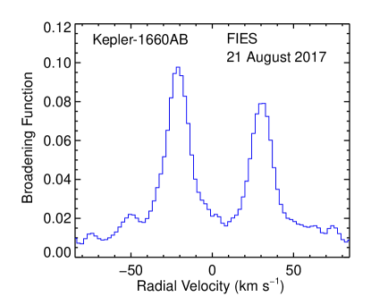
Figure 2: The broadening function (Rucinski, 1999) calculated for one of our spectroscopic observations. Two clear peaks are visible, indicating a double-lined spectroscopic binary (SB2).

2.2.3 Radial Velocity Measurements

Many of the spectra showed two sets of lines, indicating a double lined spectroscopic binary (SB2) with nearly equal mass components.

To obtain RVs from the FIES data, we used the Broadening Function technique (BF; Rucinski, 1999) on each spectral order of each of the reduced spectra. We used a Phoenix spectrum (Husser et al., 2013) with $T_{\rm eff}=6500$ K, $\log g=4.5$ and [Fe/H] $=0.0$. In the BFs two peaks are visible with similar heights and areas. This indicates that the two stars are similar in mass, in contrast to Getley et al. (2017), who derived unequal stellar masses without the benefit of high-resolution spectroscopy. One example BF is plotted in Fig. 2. For each spectral order, we fitted a double-Gaussian model and the position of the centroids of the Gaussians were then taken as RVs of the two stellar components. For each epoch, the final RVs measurements and their uncertainties were obtained from the SNR-weighted RV average and scatter obtained for the different orders.

For the CARMENES data, a TODCOR (Zucker & Mazeh, 1994) implementation was used to determine the RVs. We cross-correlated the data against the HARPS.GBOG_Procyon.txt and HARPS.GBOG_HD84937-1.fits templates from Blanco-Cuaresma et al. (2014). While the template stars have different temperatures, the fit was similar if their velocities were swapped, so we assign the output velocities to each star to result in the most coherent Keplerian motion. We set the $1\sigma$ uncertainty to 4 km/s for each CARMENES RV so that the reduced $\chi^{2}$ of the orbital fit is approximately unity.

2.3 Dynamical Model

We modeled the eclipse times and radial velocities of Kepler-1660 with a three-body model using rebound, an N-body integrator in Python (Rein & Liu, 2012). The code repository is publicly available. We used the IAS15 algorithm with adaptive step size, which is generally accurate to machine precision (Rein & Spiegel, 2015). Our algorithm assumes that mid-transit times occur when the projected separation is perpendicular to the projected velocity. Near expected eclipse times, our algorithm solves the equation $\textbf{x}\cdot\textbf{v}=0$ using the Newton-Raphson method until the step size becomes less than $10^{-10}$ d. The eclipse time is corrected for the Light Travel Time Effect (LTTE) (Borkovits et al., 2016) by adding the light travel time from the radial center-of-mass of the binary stars to the radial center-of-mass of the entire system. In practice, the LTTE ETVs have an amplitude $\sim 30$ times smaller than the dynamical ETVs.

The model has 14 free parameters. All parameters are osculating values at the epoch BJD-2454900. Two parameters, $P_{1}$ and $P_{2}$, encode the periods of the secondary star and planet, respectively. Three parameters, $M_{A}$, $M_{B}$, and $M_{p}$, give the masses of the primary, secondary, and planet. The eccentricity and argument of periapse are parametrized by $e_{1}$ and $\omega_{1}$ for the binary and $e_{2}\cos\omega_{2}$ and $e_{2}\sin\omega_{2}$ for the planet. The sky-plane inclinations are $i_{1}$ and $i_{2}$. The longitudes of the ascending node are $\Omega_{1}$ and $\Omega_{2}$, but because the data only constrain $\Delta\Omega=\Omega_{2}-\Omega_{1}$, we set $\Omega_{1}=0$ during the fitting. The phase of the binary is represented by $T_{01}$, the time of inferior conjunction assuming no planetary perturbation of the binary orbit. This time would correspond to the time of the first eclipse for a sufficiently edge on orbit, and is well-constrained by the data. The orbital phase of the planet is represented by $T_{\rm p}$, the first time after BJD-2454900 that the planet passes through periapse. The orbital elements of the secondary star are defined relative to the primary star, and those of the planet are defined relative to the center-of-mass of the primary and secondary stars. Finally, to account for the radial velocity of the system’s barycenter and because our radial velocity data were reduced separately, we include two radial velocity zero point offsets, $\gamma_{1}$ and $\gamma_{2}$ for the NOT and CARMENES data, respectively.

The model outputs eclipse times, individual stellar radial velocities at predetermined times, and the impact parameter at each eclipse. To match the simulated eclipse impact parameters to the observed $b_{0,\text{obs}}$ and $db/dt_{\text{obs}}$, we fit the simulated impact parameters to the linear model $b(t)=b_{0,\text{sim}}+db/dt_{\text{sim}}\cdot t$, where $t$ is given in BJD-2454900.

For the eclipse times, we define the goodness-of-fit statistic

$$\chi^{2}_{\text{ETV}}=\sum_{i}\left(\frac{E_{\text{mod},i}-E_{i}}{\sigma_{i}}\right)^{2}$$ (3)

where $E_{i}$, $E_{\text{mod},i}$, and $\sigma_{i}$ are the observed eclipse midpoint, modeled eclipse midpoint, and timing uncertainty of the $i$-th eclipse, respectively.

For the RV measurements of stars A and B, we define the goodness-of-fit statistic

$$\chi^{2}_{\text{RV}}=\sum_{j}\left(\frac{RV_{\text{A,mod},j}-RV_{\text{A},j}}{\sigma_{\text{A},j}}\right)^{2}+\left(\frac{RV_{\text{B,mod},j}-RV_{\text{B},j}}{\sigma_{\text{B},j}}\right)^{2}$$ (4)

where $RV_{j}$, $RV_{\text{mod},j}$, and $\sigma_{j}$ are the observed radial velocity, modeled radial velocity, and radial velocity uncertainty of the $j$-th measurement, respectively.

Finally, for the eclipse depth measurements, we define the goodness-of-fit statistic

$$\chi^{2}_{b(t)}=\left(\frac{db/dt_{\text{sim}}-db/dt_{\text{obs}}}{\sigma_{db/dt}}\right)^{2}+\left(\frac{b_{0,\text{sim}}-b_{0,\text{obs}}}{\sigma_{b_{0}}}\right)^{2}$$ (5)

where $db/dt_{\text{obs}}$ and $b_{0,\text{obs}}$ are the observed eclipse impact parameter change slope and constant with their respective uncertainties $\sigma_{db/dt}$ and $\sigma_{b_{0}}$, given in Section 2.1, and $db/dt_{\text{sim}}$ and $b_{0,\text{sim}}$ are the simulated eclipse impact parameter change slope and intercept.

From these statistics, we adopt a total log-likelihood of

$$\log\mathcal{L}=-\frac{1}{2}\chi^{2}_{\text{ETV}}-\frac{1}{2}\chi^{2}_{\text{RV}}-\frac{1}{2}\chi^{2}_{b(t)}.$$ (6)

We also set $\log\mathcal{L}=-\infty$ for samples that did not satisfy Eq. 2, i.e. there must be a primary eclipse but not a secondary one.

The Affine-Invariant MCMC Ensemble sampler from emcee was used to sample the parameter space and determine parameter uncertainties. We evolved 100 chains for 40 000 generations and removed the first 5000 as burn-in.

2.4 Isochrones Model

While eclipsing binaries usually provide an opportunity to measure absolute stellar radii, in this case the lack of secondary eclipses constrains only the ratio of radii. However, the absolute stellar masses derived from radial velocities can be used along with photometric fluxes and parallax measurements to estimate stellar radii. We modeled the pair of stars using the isochrones package and its included MIST stellar models (Morton, 2015). Because the stellar masses derived from the radial velocity fit are correlated, we parametrized the stellar mass prior as a bivariate normal distribution with means $M_{A},M_{B}$ and correlation $\rho_{M}$ given in Table 1. We also include a variety of photometric and astrometric parameters, detailed in Table 1. The model parameters were masses for each star, and a joint metallicity, age, distance, and V – band extinction. We find a primary star radius of $R_{A}=1.49\pm 0.07R_{\odot}$ and a secondary star radius of $R_{B}=1.30\pm 0.06R_{\odot}$. We use these values, without uncertainties, in the dynamical model to compute the impact parameter of each eclipse. The fit also recovers effective temperatures of the primary and secondary stars of $6050\pm 40$ K and $6040\pm 30$  K as well as a primary-to-secondary flux ratio of $1.32\pm 0.22$.

Table 1: The photometric and astrometric measurements used in the isochrones fit.

Parameter	Value	Uncertainty	Source
Parallax (milliarcsec)	0.8126	0.0148	Gaia DR2
G magnitude	13.4394	0.0002	Gaia DR2
BP magnitude	13.7217	0.0017	Gaia DR2
RP magnitude	12.9942	0.0009	Gaia DR2
J magnitude	12.499	0.023	2MASS
H magnitude	12.217	0.018	2MASS
K magnitude	12.215	0.024	2MASS
$M_{A}$ ($M_{\odot}$)	1.1366	0.0728	This work
$M_{B}$ ($M_{\odot}$)	1.0820	0.0644	This work
$\rho_{M}$	0.94504	–	This work
$R_{A}$ ($R_{\odot}$)	1.491	0.072	This work
$R_{B}$ ($R_{\odot}$)	1.299	0.061	This work

3 Results

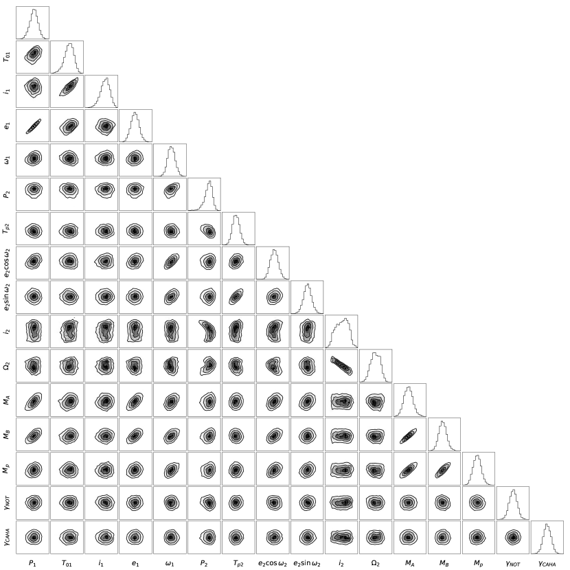
Figure 10: Scatter plot of correlations between the parameters of our model. Contour levels mark 0.5, 1, 1.5, and 2$\sigma$ bounds. See the main body for the precise parameter definitions and values.

The best-fitting solution and uncertainties derived from our MCMC chains are shown in Table 2 and parameter correlations in Fig. 10. The posterior distribution centers on a region of parameter space that closely matches the observed eclipse times, eclipse depths, and radial velocities. For our best-fitting solution, we find $\chi^{2}_{\text{ETV}}=60.90$, $\chi^{2}_{\text{RV}}=16.65$, and $\chi^{2}_{b(t)}=0.16$. The total $\chi^{2}=77.71$ is very close to 77, the degrees of freedom in the model, indicating that our solution is a satisfactory fit to the data.

The eclipse time data and our best-fitting solution are shown on an O-C diagram in Fig. 3. Both the model and data times were subtracted by the same best-fitting linear ephemeris model to emphasize the eclipse timing variations rather than the orbital period. Figure 4 contains the same data but phase-folded to the peak Fourier frequency of $235.9$ d. The double-humped structure common to ETVs caused by a third body is apparent, as is a small asymmetry in the widths of the peaks due to the eccentricity of the orbit of the third body. Also visible is a slight shift in the shape of the ETVs over the $\sim 1500$ d observation period. This is because the periapse of the planet, which has a strong effect on the ETV shape (Borkovits et al., 2016), precesses over the Kepler baseline.

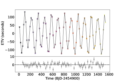
Figure 3: The Observed-Calculated primary eclipse times. Eclipse mid-times from the N-body model are the colored crosses, times from the light curve fit are the gray circles.

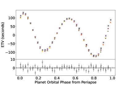
Figure 4: Same as Fig. 3 but phase-folded at the peak ETV frequency $235.9$d. Periapse precession of the planet causes the shape of the ETV curve itself to change slightly over the Kepler baseline

.

The stellar radial velocities from the dynamical fit are shown in Fig. 5. The non-zero eccentricity and near-unity mass ratio is apparent. The mass determination is hampered by limited phase sampling near the peak radial velocity; nevertheless we determine the stellar masses to better than 10 per cent. In contrast to the results of Getley et al. (2017), we find the stars to have remarkably similar masses, with $M_{A}/M_{B}=1.05\pm 0.02$.

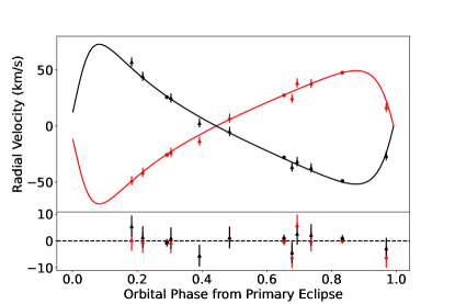
Figure 5: Radial velocity observations as a function of binary orbital phase from eclipse. Solid lines are the N-body model. Circles are the data from FIES and triangles are the data from CARMENES. The red curve is the primary star and the black curve is the secondary star.

Table 2: The results of the MCMC fit to ETVs, RVs and impact parameter measurements. The orbital elements are instantaneous (osculating) values at the reference epoch $T_{\text{ref}}=2454900\text{ BJD}$.

Parameter	Maximum Likelihood Value	Median	$1\sigma$ uncertainty
Binary Orbit
Orbital period, $P_{1}$ (d)	18.610875	18.610869	0.000031
Time of eclipse, $T_{01}$ (BJD-2454900)	66.861873	66.861694	0.000302
Eccentricity, $e_{1}$	0.5032	0.4973	0.0172
Inclination, $i_{1}$ (deg)	84.670	84.399	0.766
Argument of periapse, $\omega_{1}$ (deg)	108.34	109.09	1.79
Ascending node $\Omega_{1}$ (deg)	0.0 (fixed)	0.0	0.0
Primary star mass, $M_{A}$ $(M_{\odot})$	1.1366	1.1450	0.0728
Secondary star mass, $M_{B}$ $(M_{\odot})$	1.0820	1.0980	0.0644
Planet Orbit
Orbital period, $P_{2}$ (d)	239.4799	239.5044	0.0686
Time of periapse, $T_{P}$ (BJD-2454900)	95.811	95.730	0.815
Eccentricity, $e_{2}$	0.05511	0.05541	0.00147
Inclination, $i_{2}$	80.17	86.31	4.21
Argument of periapse, $\omega_{2}$ (deg)	-46.58	-46.17	1.87
Longitude of ascending node, $\Omega_{2}$ (deg)	0.894	-0.437	0.931
Planet mass, $M_{p}$ $(M_{\rm Jup})$	4.885	4.992	0.230
Mutual inclination, $i_{m}$ (deg)	3.35	3.71	8.21a
Barycentric radial velocity (NOT), $\gamma_{1}$ (km s-1)	4.508827	4.644869	0.550843
Barycentric radial velocity (CARMENES), $\gamma_{2}$ (km s-1)	77.427103	77.442553	1.000817
a 95% upper limit

The dynamical architecture of circumbinary systems depends strongly on the mutual inclination $i_{m}$ between the binary and circumbinary orbital planes (Farago & Laskar, 2010). This observer-independent value can be computed from angles referenced to the sky-plane by the spherical law of cosines (e.g. Borkovits et al., 2015)

$$\cos{i_{m}}=\cos{i_{1}}\cos{i_{2}}+\sin{i_{1}}\sin{i_{2}}\cos{\Delta\Omega}.$$ (7)

With such a definition, values of $i_{m}=0^{\circ}$, $90^{\circ}$, $180^{\circ}$ represent prograde coplanar, polar, and retrograde coplanar orbits, respectively. Figure 6 shows the posterior distribution of the mutual inclination as compared with the transiting circumbinary planet sample (Li et al., 2016). The distribution is consistent with coplanar and we find an 95 per cent certainty upper limit on the mutual inclination of $8.21^{\circ}$. This coplanarity is consistent with, though less precisely constrained than, the transiting circumbinary planet sample.

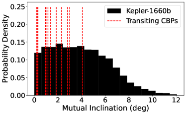
Figure 6: Posterior distribution of the planet-to-binary mutual inclination from our MCMC chains. Dashed red vertical lines mark the best-fit mutual inclinations of the 14 transiting circumbinary planets from TESS and Kepler .

3.1 Constraining alternative solutions

As noted above, the three descriptions of this system (Borkovits et al. (2016), Getley et al. (2017), and this work) differ substantially in their parameters, particularly in the orientation of the planet orbit. To better understand the possible orbital configurations, we mapped slices of the parameter space and determined which regions are consistent with the Kepler eclipse data. Our RV data and the light curve strongly constrain the orbital elements and mass of the binary, therefore we only modify the seven parameters describing the planet orbit and mass and hold the remaining ten fixed to our best-fit solution in Table 2.

Although we used the sky-plane inclination $i_{2}$ and relative longitude of ascending node $\Delta\Omega$ to parametrize the planet in the MCMC fit, here we use the more dynamically relevant mutual inclination $i_{m}$ and dynamical argument of periapse $g_{1}$. The dynamical argument of periapse, defined in Borkovits et al. (2016), is the angle between the periapse of the binary orbit and the intersection of the planet orbit with the binary orbital plane. These angles are of particular interest because fixed points in the Hamiltonian of a test particle orbiting an eccentric binary occur in four places: coplanar orbits with $i_{m}=0^{\circ},180^{\circ}$, and polar orbits $(i_{m},g_{1})=(90^{\circ},\pm 90^{\circ})$. At those points precession of the planet orbital plane vanishes (Farago & Laskar, 2010). Furthermore, circumbinary protoplanetary discs dissipatively evolve into one of these fixed points, making them likely regions for circumbinary discs and planet formation (Martin & Lubow, 2017; Kennedy et al., 2019).

First, we show which regions of the $(i_{m},g_{1})$ parameter space can produce the observed ETVs. At 5000 points uniformly distributed in the circle defined by $0^{\circ}\leq i_{m}\leq 180^{\circ}$, $0^{\circ}\leq g_{1}\leq 360^{\circ}$, we fit the 5 remaining parameters ($P_{2}$, $T_{P}$, $e_{2}\cos\omega_{2}$, $e_{2}\sin\omega_{2}$, $M_{p}$) to minimize $\chi^{2}_{\text{ETV}}$, the sum of squared normalized residuals of the eclipse times.

Second, we show which regions of the $(i_{m},g_{1})$ parameter space can produced the observed changing eclipse depth. At the same 5000 points in $(i_{m},g_{1})$ space, we compute the change in impact parameter for the $\chi^{2}_{\text{ETV}}$-minimizing solution found previously, and compare it to the measured depth change by calculating $\chi^{2}_{b(t)}$ (Eq. 5).

The results are shown in Fig. 7. The left plot shows three regions of $(i_{m},g_{1})$ parameter space that can reproduce the observed eclipse times: a large region centered around $i_{m}\approx 0^{\circ}$, and two smaller regions centered around $(i_{m},g_{1})\approx(130^{\circ},10^{\circ})$ and $(130^{\circ},190^{\circ})$. However, the right plot demonstrates that these two misaligned configurations are strongly ruled out because they result in depth variations much larger than observed. We can therefore conclude that a prograde and nearly coplanar solution is the only configuration consistent with the RV, eclipse timing, and eclipse depth data.

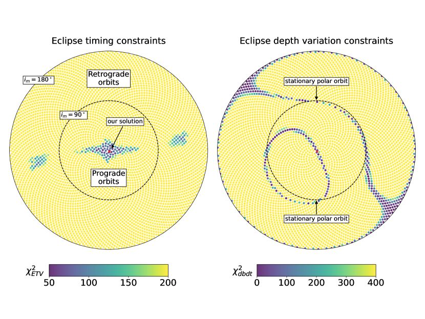
Figure 7: Constraints on planetary orientation from the eclipse timing and eclipse depth changes. On these plots, the radial coordinate is the mutual inclination, $i_{m}$, and the azimuthal coordinate is the dynamical argument of periapse, $g_{1}$, defined such that $g_{1}=0$ on the positive x-axis and increases going counterclockwise. The color of each point on the left panel is the answer to the question, “for fixed $(i_{m},g_{1})$ and binary parameters, how well could a planet reproduce the eclipse times?” Each point on the right panel uses the same best-fitting solution as the respective point on the left but is colored according to how well that solution matches the observed change in impact parameter from the light curve. On both plots, dark dots represent good fits and light dots poor ones, and the red crosses mark the $i_{m}$ and $g_{1}$ of Kepler-1660 reported by this work.

4 Discussion

4.1 Discrepancies with previous works

The initial analysis of Borkovits et al. (2016) and the follow-up work of Getley et al. (2017) both only modelled the eclipse timing variations, and not any eclipse depth variations. They also did not have the benefit of radial velocity characterization. Our RV and ETV-only model does allow for some misaligned orbits, including two patches of permissible parameter space with retrograde inclinations similar to the Getley et al. (2017) $i_{m}=120^{\circ}$ result. However, the right side of Fig. 7 demonstrates that by adding in impact parameter constraints, the Getley et al. (2017) solution is ruled out and a coplanar solution is favored. This is reiterated in the mutual inclination posterior plotted in Fig. 6.

However, our model is in rough agreement with respect to the planet’s period (239.48 d vs 237.71 d from Getley et al. 2017). Because both works report osculating (instantaneous) orbital elements, and the osculating planet period in our model varies by $\approx 8$ d over the Kepler baseline, the difference is likely attributable to the choice of reference epoch and other orbital parameters. Our mass is lower ($4.89M_{\rm Jup}$ vs $7.698M_{\rm Jup}$ from Getley et al. 2017), but still qualitatively a massive ‘super-Jupiter’. We also note that the Getley et al. (2017) best-fitting binary inclination is $80^{\circ}$, which would not correspond to an eclipsing binary.

Our work also benefits from our follow-up RVs, which the previous studies did not have at the time but encouraged. These RVs indicate a significantly different set of binary parameters. The clear signature of a double-lined spectroscopic binary reveals a near twin binary, with $M_{\rm A}=1.14M_{\odot}$ and $M_{\rm B}=1.08M_{\odot}$, as compared to the unequal masses from Getley et al. (2017) of $M_{\rm A}=1.21M_{\odot}$ and $M_{\rm B}=0.51M_{\odot}$. We also find a binary that is twice as eccentric, with $e_{1}=0.50$, compared with Getley et al. (2017)’s 0.246. Discrepancies in the stellar and binary parameters may account for their larger planet mass. Radial velocity characterization is particularly important for binaries such as Kepler-1660AB where there are no secondary eclipses, and hence very little information is known about the eccentricity and mass ratio from photometry alone. However, we note that even though RVs were essential for constraining the planet’s parameters, a highly misaligned orbit can be ruled out from the photometry alone, through the lack of eclipse depth variations.

4.2 Future observations

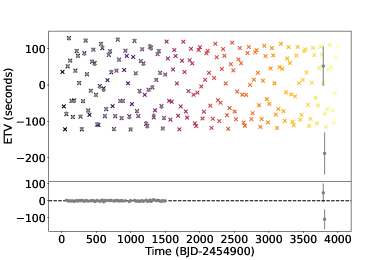
Figure 8: Model ETVs (coloured crosses) and observed ETVs (gray circles). The initial approximately four years of ETVs come from Kepler, with very small error bars. TESS has observed two eclipses, with ETVs matching the model, albeit with very large error bars. The colour of the model ETVs scales with the eclipse time.

The circumbinary planet Kepler-1660ABb could be independently detected in radial velocities using a long time series of higher precision radial velocity measurements which are sensitive to the signal of not only the binary, but of the planet itself. This was recently demonstrated with the RV detection of the transiting Kepler-16ABb (Triaud et al., 2022) and the discovery of BEBOP-1c/TOI-1338ABc in radial velocities (Standing et al., 2023).

The expected planet RV semi-amplitude for Kepler-1660ABb is $K=94$ m s^-1. Our present data are not sufficient to detect the planet mainly because our precision is on the order of km s^-1. We also only have 12 observations (equal to the number of free parameters with two Keplerian orbits) spanning 206 d (less than the 239.5 d orbit). Finally, Kepler-1660ABb is a double-lined spectroscopic binary, for which spectral contamination makes spectroscopic analysis trickier than the single-lined binaries Kepler-16ABb and BEBOP-1c/TOI-1338ABc.

An alternative way of detecting the planet is in transit. Even though the planet is currently not in transitability, the nodal precession of its orbit will change its sky orientation over time, potentially bringing it in and out of transitability. This was first proposed by Schneider (1994), studied in more detail by Martin & Triaud (2014, 2015); Martin (2017) and seen observationally for Kepler-413 (Kostov et al., 2014) and Kepler-453 (Welsh et al., 2015) discoveries. The period of this circumbinary nodal precession was derived by Farago & Laskar (2010) as a function of orbital elements and stellar masses. Using their expression we obtain $P_{\text{prec}}=86$ yr for Kepler-1660.

Martin & Triaud (2015) derived an analytic criterion for the minimum mutual inclination needed for transitability to occur on the primary (A) or secondary (B) star at some point during the nodal precession cycle:

$$i_{m,\text{min}}>\left|\frac{\pi}{2}-i_{1}\right|-\sin^{-1}\left(\frac{a_{\rm A,B}}{a_{\rm p}}\sin\left|\frac{\pi}{2}-i_{1}\right|+\frac{R_{\rm A,B}}{a_{\rm p}}\right).$$ (8)

For Kepler-1660ABb, $i_{m,\text{min}}=3.8^{\circ}$ for guaranteed transitability. Based on our current knowledge, it is not certain that the planet will ever transit. The main reason is that the binary, despite eclipsing, is $\sim 5^{\circ}$ off an exactly edge on orbit. Extending this slightly tilted orbital plane out to the distance of the planet, a planet in this plane (i.e. perfectly coplanar) would not transit. Our 95 per cent certainty upper limit to $i_{m}$ is $8.2^{\circ}$. Using Eq. 8 we find the probability of the planet ever transiting either to be 70 per cent when marginalized over our posterior distribution.

Based on a cursory look of existing TESS data, we do not see any transits. TESS has discovered two transiting circumbinary planets so far Kostov et al. (2020a, 2021) but its short one-month observing sectors present a challenge for the typically long-period circumbinary planets (Kostov et al., 2020b). The eclipses of the binary are visible in TESS and could provide an opportunity to dramatically enhance the observational baseline of this system. We have determined the mid-times for two such eclipses and found them to be consistent with our model (Figure 8) However, the far reduced photometric performance of TESS compared to Kepler means that these new data do not meaningfully improve our results.

4.3 Orbital stability

To confirm that this planet is dynamically stable, we produce a custom ‘stability map’ in Fig. 9 using the argument of periapse, period, eccentricity, and masses of the binary from Table 2. This map shows the planet’s eccentricity variation ($\log\Delta e$) for a given starting planet eccentricity and semi-major axis over an evolution time of 5000 yr. The color represents the eccentricity variation, which is indicative of stability, with bluer regions being unstable and redder regions being stable. The overlaid dashed line is the classic stability limit from Holman & Wiegert (1999), modified by Quarles et al. (2018) to account for the planet’s eccentricity. The black wedged lines are the resonant widths from Mardling (2013) and indicate how resonances can create regions of instability at very low eccentricities for lower semi-major axis values. The circumbinary planet in this system, at a semi-major axis just below 1 au with an eccentricity of 0.055, is indicated by the white circle. At this position, the planet sits comfortably in a stable orbit and further evolution will not threaten this stability.

The planet is farther away from the stability limit than most of the transiting circumbinary planets, which are typically found ‘piled-up’ near where the circumbinary disc inner edge would have been (Martin & Lubow, 2018). Like the transit method, but unlike the light travel time effect, detection by dynamically-induced ETVs will be biased towards planets closer to the binary (Borkovits et al., 2015). Ultimately, a population of circumbinary planets found with different methods will be needed to rigorously assess how piled up planets are near the stability limit. That distribution has significant implications for their formation history of circumbinary planets, as it is believed that they form in the outer regions of the disc before migrating in and parking near the disc edge (Pierens & Nelson, 2013; Penzlin et al., 2021; Martin & Fitzmaurice, 2022; Fitzmaurice et al., 2022).

Nevertheless, as an individual planet, Kepler-1660ABb fits with the Pierens & Nelson (2008) prediction that massive circumbinary planets should not be found near the stability limit. Their argument is that the parking of inwards-migrating small planets near the inner disc edge is caused by a significant density bump in the disc. If the planet is very massive (roughly Jupiter or higher) then it will open up a gap in the disc and move inward due to Type-II migration. The gap eliminates the inner pressure bump, shutting off the parking mechanism. The planet then migrates too close to the binary and gets ejected or sent on a much wider orbit. For Kepler-1660ABb to exist on its current orbit likely means the disc dissipated before it could migrate dangerously too close.

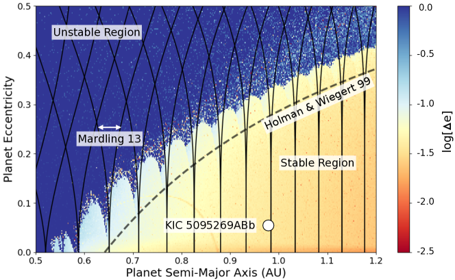
Figure 9: Stability map of planets of different orbital distance and eccentricity around the Kepler-1660AB binary. The color scale indicates $\log(\Delta e)$, the variation in eccentricity over an N-body integration time of 5000 years. Blue orbits correspond to unstable planets ejected from the system. The black solid line cones are the mean motion resonant widths from Mardling (2013), which tend to correspond to heightened eccentricity variation. The black and white dashed line corresponds to the traditional Holman & Wiegert (1999) stability limit, including an empirical scaling added by Quarles et al. (2018) to account for planet eccentricity. The white circle indicates the our derived parameters for the circumbinary planet, safely in a stable parameter space.

4.4 Formation and existence of circumbinary planets on misaligned orbits

The initial orbits for Kepler-1660 proposed by Borkovits et al. (2016); Getley et al. (2017) were highly misaligned to the binary, by $40^{\circ}$ and $120^{\circ}$ respectively. We emphasize that we rule out these orbits in favour of a coplanar one solely on the basis of the data (in particular the lack of eclipse depth variations). Our conclusion is independent of any questions of the plausibility of misaligned circumbinary orbits. Indeed, there are arguments that they may exist, as we discuss briefly here.

All of the known transiting circumbinary planets have orbits aligned to within $4^{\circ}$ of the host binary orbit (Martin & Lubow 2019 and Fig. 6). The mutual inclination distribution can be roughly described by a Rayleigh distribution with $\sigma=1.5^{\circ}$ (Martin, 2019). However, Martin & Triaud (2014) showed that transits for a misaligned orbit would be aperiodic and hard to detect, and hence this flat inclination distribution may be an observational bias. More recent work of Chen & Kipping (2022) comes to a similar conclusion. A flat inclination distribution would imply a circumbinary gas giant frequency similar to that around single stars ($\approx 5-10$ per cent, Martin & Triaud 2014; Armstrong et al. 2014). The BEBOP radial velocity survey has not found a large ‘hidden’ population of misaligned planets (Martin et al., 2019; Standing et al., 2022), despite demonstrating that circumbinary planets can be found via radial velocity monitoring of binary stars (Triaud et al., 2022; Standing et al., 2023).

It is possible that even if the majority of circumbinary planets are coplanar, exceptional cases of misaligned orbits may exist. There are in fact multiple arguments for the existence of misalignments. From an orbital stability perspective, Pilat-Lohinger et al. (2003); Farago & Laskar (2010); Doolin & Blundell (2011); Martin & Triaud (2016) demonstrated that circumbinary planets may be stable at all mutual inclinations, including retrograde orbits. We have observed circumbinary discs that are misaligned (e.g. KH15D, Winn et al. 2004; Chiang & Murray-Clay 2004) and polar (99 Herculis, Kennedy et al. 2012, and HD 98800, Kennedy et al. 2019). Theory suggests that protoplanetary discs may form with an initially isotropic distribution but reach equilibrium states that are either coplanar or polar (Martin & Lubow, 2017, 2019). Terrestrial planet formation is theoretically possible in such polar discs (Childs & Martin, 2021), although recent work by Childs & Martin (2022) suggests that formation in a misaligned disc may lead to coplanar planets if the disc lacks gas.

Even if a planet formed in a fairly flat orbit, it is possible that planet-planet scattering could place it onto a misaligned orbit (Chatterjee et al., 2008), although there is a risk that scattering may increase not only inclination but eccentricity, potentially ejecting the planet in a binary (Smullen et al., 2016; Fitzmaurice et al., 2022). Misaligned orbits may also be produced via secular interactions with an external stellar perturber (Martin et al., 2015).

Overall, while the orbit of Kepler-1660ABb is not misaligned to its binary, such a system is far from inconceivable and we encourage continued searches for one.

5 Conclusion

We confirm the existence of a coplanar circumbinary planet Kepler-1660ABb, the first confirmed non-transiting Kepler circumbinary planet. It is a ‘super-Jupiter’, with $M_{\rm p}=4.89M_{\rm Jup}$. It was first identified using ETVs by Borkovits et al. (2016) and later analysed by Getley et al. (2017). Whereas these two studies proposed a highly misaligned planetary orbit (roughly $40^{\circ}$ and $120^{\circ}$ of misalignment, respectively), we demonstrate that the planet is in fact coplanar (to within $\approx 8^{\circ}$). Our analysis improves upon previous works by accounting for both eclipse timing variations and eclipse depth variations, the latter of which rule out a misaligned orbit because there is negligible depth variation. We also include follow-up radial velocities which we took, which allow us to properly measure the stellar masses and binary eccentricity.

Kepler-1660ABb is the most massive circumbinary planet known, but it turns out not to be the first on a significantly misaligned orbit.

Data Availability

The eclipse and radial velocity data are included in the article appendix. Posterior samples will be shared on reasonable request to the corresponding author.

Appendix A

Table 3: Eclipse mid-times from our analysis of the Kepler light curve.

Eclipse Index	Eclipse Time (BJD-2454900)	$1\sigma$ uncertainty (d)
-40	66.8651676	0.0000271
-39	85.4786256	0.0000278
-38	104.0914523	0.0000267
-37	122.7027159	0.0000264
-36	141.3133773	0.0000265
-35	159.9248384	0.0000266
-34	178.5372897	0.0000253
-33	197.1502183	0.0000268
-32	215.7628265	0.0000261
-31	234.3746132	0.0000271
-30	252.9857246	0.0000306
-29	271.5966131	0.0000270
-28	290.2081810	0.0000272
-27	308.8210001	0.0000311
-26	327.4344698	0.0000276
-25	346.0468713	0.0000276
-24	364.6577455	0.0000276
-23	383.2685300	0.0000272
-21	420.4930974	0.0000075
-20	439.1059939	0.0000299
-19	457.7183260	0.0000279
-18	476.3298060	0.0000259
-17	494.9407861	0.0000298
-16	513.5518408	0.0000265
-14	550.7769189	0.0000301
-13	569.3902668	0.0000275
-12	588.0021224	0.0000273
-11	606.6126901	0.0000273
-10	625.2238455	0.0000261
-9	643.8360273	0.0000271
-7	681.0616729	0.0000270
-6	699.6737434	0.0000302
-5	718.2850490	0.0000278
-3	755.5071126	0.0000301
-2	774.1195116	0.0000272
-1	792.7329129	0.0000273
0	811.3458716	0.0000269
1	829.9571616	0.0000274
2	848.5678133	0.0000348
3	867.1792408	0.0000267
4	885.7917271	0.0000265
6	923.0172498	0.0000268
9	978.8509935	0.0000262
10	997.4625919	0.0000267
13	1053.3012928	0.0000278
14	1071.9121903	0.0000279
15	1090.5229339	0.0000279
16	1109.1347480	0.0000280
17	1127.7474789	0.0000312
18	1146.3604138	0.0000263
19	1164.9727660	0.0000284
20	1183.5842367	0.0000284
22	1220.8063003	0.0000300
23	1239.4181253	0.0000273
24	1258.0312472	0.0000291
25	1276.6446312	0.0000269
26	1295.2564795	0.0000270
27	1313.8672377	0.0000267
28	1332.4782956	0.0000297

Table 4: continued

Eclipse Index	Eclipse Time (BJD-2454900)	$1\sigma$ uncertainty (d)
30	1369.7033394	0.0000277
31	1388.3161322	0.0000301
32	1406.9281795	0.0000280
33	1425.5394157	0.0000316
34	1444.1502984	0.0000297
35	1462.7615862	0.0000311
36	1481.3738519	0.0000279
37	1499.9872078	0.0000278

Table 5: Our radial velocity data. All velocities are given in km s^-1, and errors are $1\sigma$ uncertainties.

Time (BJD-2454900)	Primary RV	Primary RV Error	Secondary RV	Secondary RV uncertainty	Telescope
3087.429909	-21.1	1.2	30.3	1.3	NOT/FIES
3131.385773	32.0	1.2	-23.5	1.4	NOT/FIES
3153.353683	52.3	1.1	-44.4	1.4	NOT/FIES
3299.647071	116.4	4.0	46.3	4.0	CARMENES
3312.647215	64.6	4.0	80.6	4.0	CARMENES
3329.620515	54.5	4.0	103.0	4.0	CARMENES
3336.578951	102.6	4.0	41.3	4.0	CARMENES
3346.610853	36.6	4.0	122.4	4.0	CARMENES
3351.600984	85.1	4.0	73.1	4.0	CARMENES
3360.605952	94.6	4.0	51.3	4.0	CARMENES
3364.585143	29.1	4.0	135.1	4.0	CARMENES
3393.510143	115.9	4.0	40.6	4.0	CARMENES

References

- Applegate (1992) Applegate J. H., 1992, The Astrophysical Journal, 385, 621
- Armstrong et al. (2013) Armstrong D., et al., 2013, Monthly Notices of the Royal Astronomical Society, 434, 3047
- Armstrong et al. (2014) Armstrong D. J., Osborn H. P., Brown D. J. A., Faedi F., Gómez Maqueo Chew Y., Martin D. V., Pollacco D., Udry S., 2014, Monthly Notices of the Royal Astronomical Society, 444, 1873
- Blanco-Cuaresma et al. (2014) Blanco-Cuaresma S., Soubiran C., Jofré P., Heiter U., 2014, Astronomy and Astrophysics, 566, A98
- Borkovits et al. (2015) Borkovits T., Rappaport S., Hajdu T., Sztakovics J., 2015, Monthly Notices of the Royal Astronomical Society, 448, 946
- Borkovits et al. (2016) Borkovits T., Hajdu T., Sztakovics J., Rappaport S., Levine A., Bíró I. B., Klagyivik P., 2016, Monthly Notices of the Royal Astronomical Society, 455, 4136
- Bours et al. (2016) Bours M. C. P., et al., 2016, Monthly Notices of the Royal Astronomical Society, 460, 3873
- Chatterjee et al. (2008) Chatterjee S., Ford E. B., Matsumura S., Rasio F. A., 2008, The Astrophysical Journal, 686, 580
- Chen & Kipping (2022) Chen Z., Kipping D., 2022, Monthly Notices of the Royal Astronomical Society, 513, 5162
- Chiang & Murray-Clay (2004) Chiang E. I., Murray-Clay R. A., 2004, The Astrophysical Journal, 607, 913
- Childs & Martin (2021) Childs A. C., Martin R. G., 2021, The Astrophysical Journal, 920, L8
- Childs & Martin (2022) Childs A. C., Martin R. G., 2022, The Astrophysical Journal, 927, L7
- Doolin & Blundell (2011) Doolin S., Blundell K. M., 2011, Monthly Notices of the Royal Astronomical Society, 418, 2656
- Farago & Laskar (2010) Farago F., Laskar J., 2010, Monthly Notices of the Royal Astronomical Society, 401, 1189
- Fitzmaurice et al. (2022) Fitzmaurice E., Martin D. V., Fabrycky D. C., 2022, Monthly Notices of the Royal Astronomical Society, 512, 5023
- Getley et al. (2017) Getley A. K., Carter B., King R., O’Toole S., 2017, Monthly Notices of the Royal Astronomical Society, 468, 2932
- Hamers & Portegies Zwart (2016) Hamers A. S., Portegies Zwart S. F., 2016, Monthly Notices of the Royal Astronomical Society, 459, 2827
- Hardy et al. (2015) Hardy A., et al., 2015, The Astrophysical Journal, 800, L24
- Hinse et al. (2014) Hinse T. C., Lee J. W., Goździewski K., Horner J., Wittenmyer R. A., 2014, Monthly Notices of the Royal Astronomical Society, 438, 307
- Holman & Wiegert (1999) Holman M. J., Wiegert P. A., 1999, The Astronomical Journal, 117, 621
- Horner et al. (2013) Horner J., Wittenmyer R. A., Hinse T. C., Marshall J. P., Mustill A. J., Tinney C. G., 2013, Monthly Notices of the Royal Astronomical Society, 435, 2033
- Husser et al. (2013) Husser T.-O., Wende-von Berg S., Dreizler S., Homeier D., Reiners A., Barman T., Hauschildt P. H., 2013, Astronomy and Astrophysics, 553, A6
- Kennedy et al. (2012) Kennedy G. M., et al., 2012, Monthly Notices of the Royal Astronomical Society, 421, 2264
- Kennedy et al. (2019) Kennedy G. M., et al., 2019, Nature Astronomy, 3, 230
- Kostov et al. (2014) Kostov V. B., et al., 2014, The Astrophysical Journal, 784, 14
- Kostov et al. (2020a) Kostov V. B., et al., 2020a, The Astronomical Journal, 159, 253
- Kostov et al. (2020b) Kostov V. B., et al., 2020b, The Astronomical Journal, 160, 174
- Kostov et al. (2021) Kostov V. B., et al., 2021, The Astronomical Journal, 162, 234
- Li et al. (2016) Li G., Holman M. J., Tao M., 2016, The Astrophysical Journal, 831, 96
- Mandel & Agol (2002) Mandel K., Agol E., 2002, The Astrophysical Journal, 580, L171
- Mardling (2013) Mardling R. A., 2013, Monthly Notices of the Royal Astronomical Society, 435, 2187
- Martin (2017) Martin D. V., 2017, Monthly Notices of the Royal Astronomical Society, 465, 3235
- Martin (2018) Martin D. V., 2018, Populations of Planets in Multiple Star Systems, doi:10.1007/978-3-319-55333-7_156.
- Martin (2019) Martin D. V., 2019, Monthly Notices of the Royal Astronomical Society, 488, 3482
- Martin & Fabrycky (2021) Martin D. V., Fabrycky D. C., 2021, The Astronomical Journal, 162, 84
- Martin & Fitzmaurice (2022) Martin D. V., Fitzmaurice E., 2022, Monthly Notices of the Royal Astronomical Society, 512, 602
- Martin & Lubow (2017) Martin R. G., Lubow S. H., 2017, The Astrophysical Journal Letters, 835, L28
- Martin & Lubow (2018) Martin R. G., Lubow S. H., 2018, Monthly Notices of the Royal Astronomical Society, 479, 1297
- Martin & Lubow (2019) Martin R. G., Lubow S. H., 2019, Monthly Notices of the Royal Astronomical Society, 490, 1332
- Martin & Triaud (2014) Martin D. V., Triaud A. H. M. J., 2014, Astronomy and Astrophysics, 570, A91
- Martin & Triaud (2015) Martin D. V., Triaud A. H. M. J., 2015, Monthly Notices of the Royal Astronomical Society, 449, 781
- Martin & Triaud (2016) Martin D. V., Triaud A. H. M. J., 2016, Monthly Notices of the Royal Astronomical Society, 455, L46
- Martin et al. (2015) Martin D. V., Mazeh T., Fabrycky D. C., 2015, Monthly Notices of the Royal Astronomical Society, 453, 3554
- Martin et al. (2019) Martin D. V., et al., 2019, Astronomy and Astrophysics, 624, A68
- Morton (2015) Morton T. D., 2015, Astrophysics Source Code Library, p. ascl:1503.010
- Muñoz & Lai (2015) Muñoz D. J., Lai D., 2015, Proceedings of the National Academy of Science, 112, 9264
- Penzlin et al. (2021) Penzlin A. B. T., Kley W., Nelson R. P., 2021, Astronomy and Astrophysics, 645, A68
- Pierens & Nelson (2008) Pierens A., Nelson R. P., 2008, Astronomy and Astrophysics, 483, 633
- Pierens & Nelson (2013) Pierens A., Nelson R. P., 2013, Astronomy and Astrophysics, 556, A134
- Pilat-Lohinger et al. (2003) Pilat-Lohinger E., Funk B., Dvorak R., 2003, Astronomy and Astrophysics, 400, 1085
- Prša et al. (2011) Prša A., et al., 2011, The Astronomical Journal, 141, 83
- Pulley et al. (2022) Pulley D., Sharp I. D., Mallett J., von Harrach S., 2022, Monthly Notices of the Royal Astronomical Society, 514, 5725
- Qian et al. (2009) Qian S. B., Dai Z. B., Liao W. P., Zhu L. Y., Liu L., Zhao E. G., 2009, The Astrophysical Journal, 706, L96
- Quarles et al. (2018) Quarles B., Satyal S., Kostov V., Kaib N., Haghighipour N., 2018, The Astrophysical Journal, 856, 150
- Quirrenbach et al. (2014) Quirrenbach A., et al., 2014, in Ground-Based and Airborne Instrumentation for Astronomy V. SPIE, p. 91471F, doi:10.1117/12.2056453
- Rabago et al. (2023) Rabago I., Zhu Z., Martin R. G., Lubow S. H., 2023, Monthly Notices of the Royal Astronomical Society, 520, 2138
- Rein & Liu (2012) Rein H., Liu S.-F., 2012, Astronomy and Astrophysics, 537, A128
- Rein & Spiegel (2015) Rein H., Spiegel D. S., 2015, Monthly Notices of the Royal Astronomical Society, 446, 1424
- Rucinski (1999) Rucinski S., 1999, in IAU Colloq. 170: Precise Stellar Radial Velocities. eprint: arXiv:astro-ph/9807327, p. 82, doi:10.48550/arXiv.astro-ph/9807327
- Schneider (1994) Schneider J., 1994, Planetary and Space Science, 42, 539
- Smullen et al. (2016) Smullen R. A., Kratter K. M., Shannon A., 2016, Monthly Notices of the Royal Astronomical Society, 461, 1288
- Standing et al. (2022) Standing M. R., et al., 2022, Monthly Notices of the Royal Astronomical Society, 511, 3571
- Standing et al. (2023) Standing M. R., et al., 2023, Nature Astronomy, 7, 702
- Telting et al. (2014) Telting J. H., et al., 2014, Astronomische Nachrichten, 335, 41
- Triaud et al. (2022) Triaud A. H. M. J., et al., 2022, Monthly Notices of the Royal Astronomical Society, 511, 3561
- Welsh & Orosz (2018) Welsh W. F., Orosz J. A., 2018, Two Suns in the Sky: The Kepler Circumbinary Planets, doi:10.1007/978-3-319-55333-7_34.
- Welsh et al. (2015) Welsh W. F., et al., 2015, The Astrophysical Journal, 809, 26
- Windemuth et al. (2019) Windemuth D., Agol E., Carter J., Ford E. B., Haghighipour N., Orosz J. A., Welsh W. F., 2019, Monthly Notices of the Royal Astronomical Society, 490, 1313
- Winn et al. (2004) Winn J. N., Holman M. J., Johnson J. A., Stanek K. Z., Garnavich P. M., 2004, The Astrophysical Journal, 603, L45
- Wittenmyer et al. (2013) Wittenmyer R. A., Horner J., Marshall J. P., 2013, Monthly Notices of the Royal Astronomical Society, 431, 2150
- Zorotovic & Schreiber (2013) Zorotovic M., Schreiber M. R., 2013, Astronomy and Astrophysics, 549, A95
- Zucker & Mazeh (1994) Zucker S., Mazeh T., 1994, The Astrophysical Journal, 420, 806