A mixed and hybrid PML formulation for the 2D three-field dynamic poroelastic equations

Abstract

Simulation of wave propagation in poroelastic half-spaces presents a common challenge in fields like geomechanics and biomechanics, requiring Absorbing Boundary Conditions (ABCs) at the semi-infinite space boundaries. Perfectly Matched Layers (PML) are a popular choice due to their excellent wave absorption properties. However, PML implementation can lead to problems with unknown stresses or strains, time convolutions, or PDE systems with Auxiliary Differential Equations (ADEs), which increases computational complexity and resource consumption.

This article presents two new PML formulations for arbitrary poroelastic domains. The first formulation is a fully-mixed form that employs time-history variables instead of ADEs, reducing the number of unknowns and mathematical operations. The second formulation is a hybrid form that restricts the fully-mixed formulation to the PML domain, resulting in smaller matrices for the solver while preserving governing equations in the interior domain. The fully-mixed formulation introduces three scalar variables over the whole domain, whereas the hybrid form confines them to the PML domain.

The proposed formulations were tested in three numerical experiments in geophysics using realistic parameters for soft sites with free surfaces. The results were compared with numerical solutions from extended domains and simpler ABCs, such as paraxial approximation, demonstrating the accuracy, efficiency, and precision of the proposed methods. The article also discusses the applicability of these methods to complex media and their extension to the Multiaxial PML formulation.

The codes for the simulations are available for download from https://github.com/hmella/POROUS-HYBRID-PML.

1 Introduction

Fluid-saturated porous media are a common occurrence in nature. For instance, soils and rocks are often saturated with water in practical cases, while living tissues are saturated with blood and air. In both cases, if the solid skeleton’s displacements and strains are relatively small, linear elasticity provides an accurate representation of the underlying dynamics. Additionally, when loads are applied quickly and inertial forces play a significant role, a proper modeling strategy for wave propagation in poroelastic media is necessary. As noted by Zienkiewicz et al. [41], Biot’s poroelastic theory can be employed to describe wave propagation in poroelastic media, such as in problems of traffic-induced vibrations or geophysical applications involving seismic wave propagation. The main challenge in these types of problems is properly handling outgoing waves. In the directions where outgoing waves travel, finite energy considerations lead to the so-called “radiation conditions” towards infinity, which are used by Integral Equations or Boundary-Element methods to determine Green kernels and solve the problem rigorously. However, these conditions are often difficult to calculate and are limited to homogeneous and isotropic material properties at infinity [20]. An alternative solution is to use a foam-like subdomain to confine the region of interest, creating virtual windows in space to focus computational efforts on a specific area of the problem. The subdomain must effectively absorb the outgoing waves from the virtual window.

Numerous numerical methods have been proposed as Absorbing Boundary Conditions (ABCs). Local ABCs are often used for dry elastic problems or single-phase media due to their ease of implementation and local character in both time and space [24]. However, fluid-saturated porous media or two-phase media presents a different challenge due to an interaction between the solid skeleton and fluid flow, which depends on the loading rate. According to Biot’s theory, high-frequency loading generates two dilatational waves and one shear wave. When the porous media has low permeability and the loading is within the low frequency range, the fluid’s relative motion with respect to the soil is negligible, and viscous coupling dampens out the second dilatational wave [9, 16]. In this case, the fluid-saturated porous media behaves like a single-phase medium, where only one dilatational and one shear wave propagate.

In recent decades, the Perfectly Matched Layer (PML) has gained popularity as an ABC due to its excellent energy-absorbing properties. PML was first developed by Berenger [8] in the context of electromagnetism. Although the initial development was for Maxwell’s equations, its use as an ABC for acoustic [35], elastic [11], and poroelastic [38] domains was later extended. Since then, the technique has been widely used to simulate the propagation of elastic [28, 37, 7, 13, 26, 27, 18, 40] and poroelastic waves [36, 30, 22, 21] and new and novel formulations have been introduced. These forms can be divided into split-field and unsplit-field approaches, both of which have drawbacks. Split-field formulations often result in mixed problems where stresses or strains are unknowns, increasing the computational cost of solving the problem [15, 38, 39, 17]. Unsplit-field formulations typically require the estimation of convolutions or solving Auxiliary Differential Equations (ADEs) [30, 22], which can also be expensive due to the increased number of mathematical operations or the introduction of auxiliary variables. Additionally, little attention has been paid to simulating poroelastic waves in arbitrary domains with realistic subsoil properties.

In this article, we propose two new formulations of the Perfectly Matched Layer (PML) method for the second order three-field Biot’s equations to address the previously mentioned limitations. Our fully-mixed and hybrid formulations maintain the second-order in time structure of the original equations, which makes them compatible with most time integration schemes. Furthermore, both methods only introduce three additional scalar variables, which is at least 50% less computationally expensive than previous developments [22]. The hybrid formulation modifies Biot’s equations only in the PML region, resulting in significant computational cost savings. Our proposed methods perform well under challenging conditions, such as free-surface wave propagation, transitions between water and air-filled soft media, and complex geometries, making them suitable for simulating realistic media.

2 Poro-elastodynamic equations

The three-field model proposed by Biot [10, 41, 42] considers a domain $\Omega\subseteq\mathbb{R}^{2}$ where the solid displacement $\boldsymbol{u}(\boldsymbol{x},t)$, the displacement of the fluid phase relative to the solid $\boldsymbol{w}(\boldsymbol{x},t)$, and the pore pressure in the fluid $p(\boldsymbol{x},t)$ interacts at any position $\boldsymbol{x}$ and time $t$ such that $(\boldsymbol{x},t)\in\Omega\times T$ with $T=\left(0,\infty\right)$, according to:

$$\rho\,\ddot{\boldsymbol{u}}+\rho_{f}\,\ddot{\boldsymbol{w}} =\nabla\cdot\boldsymbol{\sigma} \quad\text{in }\Omega\times T$$ (1a)

$$\rho_{f}\,\ddot{\boldsymbol{u}}+\rho_{w}\,\ddot{\boldsymbol{w}}+\frac{\eta}{\kappa}\dot{\boldsymbol{w}} =-\nabla p \quad\text{in }\Omega\times T$$ (1b)

$$-\dot{p} =\nabla\cdot\left\{M(\alpha\dot{\boldsymbol{u}}+\dot{\boldsymbol{w}})\right\} \quad\text{in }\Omega\times T$$ (1c)

where the effective density $\rho=\rho_{s}(1-\phi)+\rho_{f}\phi\;$ depends on the solid $(\rho_{s})$ and fluid densities $(\rho_{f})$, as well as the porosity $\phi$. The fluid density $\rho_{w}=\tau\rho_{f}/\phi$ depends on the tortuosity $\tau$, the dynamic viscosity of the fluid $\eta$, and the saturated permeability of the porous media $\kappa$. The parameter $\alpha$ represents the Biot-Willis coefficient and $M$ the fluid-solid coupling bulk modulus, defined as

$$\alpha=1-\frac{K_{b}}{K_{s}},\quad M=\left(\frac{\phi}{K_{f}}+\frac{\alpha-\phi}{K_{s}}\right)^{-1}$$ (2)

where $K_{b}$, $K_{s}$, $K_{f}$ are the bulk moduli of the dry porous skeleton, solid, and fluid, respectively.

The constitutive law for the poroelastic media in (1) is given by

$$\boldsymbol{\sigma}(\boldsymbol{u},p) =C\mathbf{e}(\boldsymbol{u})-\alpha p\textbf{I}$$ (3a)

$$\mathbf{e}(\boldsymbol{u}) =\frac{1}{2}\left\{\nabla\boldsymbol{u}+(\nabla\boldsymbol{u})^{T}\right\}$$ (3b)

where $C$ is the fourth-order elastic tensor with components $C_{ijkl}=\lambda_{b}\delta_{ij}\delta_{kl}+\mu_{b}(\delta_{ik}\delta_{jl}+\delta_{il}\delta_{jk})$ (with $\delta_{ij}$ the Kronecker delta), $\mathbf{e}$ the linear strain tensor, and I the identity tensor.

The domain $\Omega$ is intended to be an unbounded semi-space, with the top boundary consisting of two parts: $\Gamma=\Gamma_{N}\cup\Gamma_{g}$. The free surface, denoted by $\Gamma_{N}$, is the region where tractions must vanish [33]. On the other hand, $\Gamma_{g}$ is the part of the top boundary where an external load $\boldsymbol{g}$ is being applied. Therefore, the boundary conditions of the problem are:

$$\boldsymbol{\sigma}(\boldsymbol{u},p)\cdot\boldsymbol{n} =\boldsymbol{g}\quad\text{in }\Gamma_{g}\times T$$ (4a)

$$\boldsymbol{\sigma}(\boldsymbol{u},p)\cdot\boldsymbol{n} =\boldsymbol{0}\quad\text{in }\Gamma_{N}\times T$$ (4b)

$$p =0\quad\text{in }\Gamma_{N}\times T$$ (4c)

The variables $\boldsymbol{u}$, $\boldsymbol{w}$, and $p$ must vanish as the distance from the source tends to infinity.

3 Derivation of PML formulas

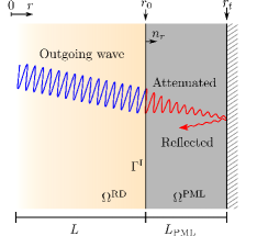
(a)

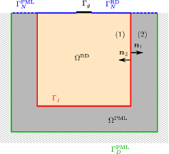
(b)

Figure 1: (a) Semi-infinite domain $\Omega$ and (b) truncated regular and PML domains $\Omega^{\text{RD}}$ and $\Omega^{\text{PML}}$ respectively.

The region of interest where boundary-reflected waves are not desired (namely Regular Domain) $\Omega^{\text{RD}}$ is surrounded and truncated by a thin Perfectly Matched Layer $\Omega^{\text{PML}}$ such that $\Omega=\Omega^{\text{RD}}\cup\Omega^{\text{PML}}$ (see Figure 1b). Thus, $\Omega^{\text{PML}}$ is defined as an extension of $\Omega^{\text{RD}}$ where the outgoing waves are attenuated by a complex coordinate stretching (see Figure 1).

3.1 Complex-coordinate stretching

A complex-coordinate stretching applied to Biot’s equations (1) leads to a modified set of equations within $\Omega$. Thus, the complex-coordinate stretching follows:

$$r\longmapsto\int_{0}^{r}\varepsilon_{r}(r^{\prime},s)~{}dr^{\prime}$$ (5)

where $r$ denotes the spatial coordinate being transformed (namely $x$ or $y$ in the two-dimensional case), $s$ the dual variable of the time in the Laplace domain, and $\varepsilon_{r}$ a complex-coordinate stretching function along the coordinate $r$. The coordinate transformation given in (5) implies:

$$\frac{\partial}{\partial r}\longmapsto\frac{1}{\varepsilon_{r}(r)}\frac{\partial}{\partial r}$$ (6)

which is the fundamental relation used to transform the governing equations.

The function $\varepsilon_{r}$ in (7) can adopt diverse forms to achieve different absorption properties. For instance, Kuzuoglu and Mitra [28] introduced the Convolutional Frequency Shifted (CFS) PML method by defining a frequency-dependent stretching function to improve the absorption efficiency at different frequencies and also to improve the time stability. Later, Correia and Jin [13] introduced the higher-order PML with a better absorption rate than CFS-PML. However, both approaches make the real and imaginary parts of $\varepsilon_{r}$ frequency-dependent, leading to convolution terms in the PML formulation. Later, Meza-Fajardo and Papageorgiou developed the Multiaxial PML (M-PML) method [32] and introduced multi-directional attenuation functions with better time stability properties. Recently, François et al. [18] proposed a non-convolutional version of the CFS-PML method in elastodynamics by introducing auxiliary variables. A standard selection for $\varepsilon_{r}$ would be:

$$\varepsilon_{r}(r,s)=\alpha_{r}(r)+\frac{\beta_{r}(r)}{s},$$ (7)

with $\alpha_{r}$ and $\beta_{r}$ denoting real-valued scaling and attenuation functions, respectively.

The real part of $\varepsilon_{r}$ scales the spatial coordinate $r$ while the imaginary part is responsible for the amplitude decay of the waves entering the PML region (see Figure 1). To avoid modifying the propagating waves inside $\Omega^{\text{RD}}$ and ensure the wave attenuation inside $\Omega^{\text{PML}}$, the following conditions must be fulfilled: $\alpha_{r}(r)$ and $\beta_{r}(r)$ are constant inside $\Omega^{\text{RD}}$ and take values of $1$ and $0$ respectively, and both functions increases monotonically with $r$ within $\Omega^{\text{PML}}$. Several ways of defining $\alpha_{r}$ and $\beta_{r}$ have been proposed in the literature in different contexts [8, 12, 26, 22], but in this investigation, polynomial profiles were chosen according to:

$$\alpha_{r}(r) =\left\{\begin{array}[]{cl}1&\text{if }0\leq r\leq r_{0}\\ 1+\alpha_{0}\left\{\frac{(r-r_{0})n_{r}}{L_{\text{PML}}}\right\}^{m}&\text{if }r_{0}\leq r\leq r_{t}\end{array}\right.$$ (8c)

$$\beta_{r}(r) =\left\{\begin{array}[]{cc}0&\text{if }0\leq r\leq r_{0}\\ \beta_{0}\left\{\frac{(r-r_{0})n_{r}}{L_{\text{PML}}}\right\}^{m}&\text{if }r_{0}\leq r\leq r_{t}\end{array}\right.$$ (8f)

where $n_{r}$ denotes the $r$-th component of the outward normal to the interface between $\Omega^{\text{RD}}$ and $\Omega^{\text{PML}}$, $L_{\text{PML}}$ the width of the PML layer, and $m$ the order of the attenuation profiles, $r_{0}$ and $r_{t}$ represent the start and end of the absorbing layer (see Figure 1). The constants $\alpha_{0}$ and $\beta_{0}$ define the absorption rate in $\Omega^{\text{PML}}$, and can be chosen as [26]:

$$\alpha_{0}=\frac{(m+1)b}{2L_{\text{PML}}}\log\left(\frac{1}{|R|}\right),\qquad\beta_{0}=\frac{(m+1)c}{2L_{\text{PML}}}\log\left(\frac{1}{|R|}\right)$$ (9)

where $b$ denotes a characteristic length (e.g., the width of the distributed load applied in the Neumann boundary or the cell size of the finite element mesh), $c_{p}$ the propagation velocity of the fastest wave, and $R$ a reflection coefficient.

3.2 PML derivation in the Laplace domain

The complex-coordinate stretching is enforced by introducing the relation (6) into the Laplace-transformed motion equations. Applying the Laplace transform to Biot’s equations leads:

$$s^{2}\rho\hat{\boldsymbol{u}}+s^{2}\rho_{f}\hat{\boldsymbol{w}} =\nabla\cdot\hat{\boldsymbol{\sigma}}$$ (linear momentum conservation) (10a)

$$s^{2}\rho_{f}\hat{\boldsymbol{u}}+s^{2}\rho_{w}\hat{\boldsymbol{w}}+s\frac{\eta}{\kappa}\hat{\boldsymbol{w}} =-\nabla\hat{p}$$ (Darcy law) (10b)

$$-s\hat{p} =\nabla\cdot\left\{M(\alpha s\hat{\boldsymbol{u}}+s\hat{\boldsymbol{w}})\right\}$$ (10c)

$$\hat{\boldsymbol{\sigma}} =C\hat{\mathbf{e}}-\alpha\hat{p}\textbf{I}$$ (constitutive relations) (10d)

$$\hat{\mathbf{e}} =\frac{1}{2}\left\{\nabla\hat{\boldsymbol{u}}+(\nabla\hat{\boldsymbol{u}})^{T}\right\}$$ (10e)

where $\hat{f}$ denotes the variable $f$ in the Laplace domain.

3.2.1 Linear momentum conservation

Replacing (6) into (10a) for the plane strain case gives:

$$s^{2}\rho\hat{u}_{x}+s^{2}\rho_{f}\hat{w}_{x} =\frac{1}{\varepsilon_{x}}\frac{\partial\sigma_{xx}}{\partial x}+\frac{1}{\varepsilon_{y}}\frac{\partial\sigma_{xy}}{\partial y}-\frac{1}{\varepsilon_{x}}\frac{\partial\alpha\hat{p}}{\partial x}$$ (11a)

$$s^{2}\rho\hat{u}_{y}+s^{2}\rho_{f}\hat{w}_{y} =\frac{1}{\varepsilon_{x}}\frac{\partial\sigma_{yx}}{\partial x}+\frac{1}{\varepsilon_{y}}\frac{\partial\sigma_{yy}}{\partial y}-\frac{1}{\varepsilon_{y}}\frac{\partial\alpha\hat{p}}{\partial y}$$ (11b)

which after multiplying both equations by $\varepsilon_{x}\varepsilon_{y}$, introducing the variables $a=\alpha_{x}\alpha_{y}$, $b=\alpha_{x}\beta_{y}+\alpha_{y}\beta_{x}$, $c=\beta_{x}\beta_{y}$, and rearranging terms can be rewritten as:

$$(s^{2}a+sb+c)(\rho\hat{\boldsymbol{u}}+\rho_{f}\hat{\boldsymbol{w}})=\nabla\cdot\left\{\boldsymbol{\sigma}(\boldsymbol{u},p)\left(\boldsymbol{\Lambda}_{e}+\frac{1}{s}\boldsymbol{\Lambda}_{p}\right)\right\}$$ (12)

where the tensors $\boldsymbol{\Lambda}_{e}$ and $\boldsymbol{\Lambda}_{p}$ are defined as

$$\left[\begin{array}[]{cc}\alpha_{y}&0\\ 0&\alpha_{x}\end{array}\right]+\frac{1}{s}\left[\begin{array}[]{cc}\beta_{y}&0\\ 0&\beta_{x}\end{array}\right]=\boldsymbol{\Lambda}_{e}+\frac{1}{s}\boldsymbol{\Lambda}_{p}$$ (13)

3.2.2 Darcy equation

Proceeding similarly with (10b) results in:

$$s^{2}\rho_{f}\hat{u}_{x}+s^{2}\rho_{w}\hat{w}_{x}+s\frac{\eta}{\kappa}\hat{w}_{x} =-\frac{1}{\varepsilon_{x}}\frac{\partial\hat{p}}{\partial x}$$ (14a)

$$s^{2}\rho_{f}\hat{u}_{y}+s^{2}\rho_{w}\hat{w}_{y}+s\frac{\eta}{\kappa}\hat{w}_{y} =-\frac{1}{\varepsilon_{y}}\frac{\partial\hat{p}}{\partial y}$$ (14b)

which after multiplying the first equation by $\varepsilon_{x}$ and the second by $\varepsilon_{y}$ lead to the following modified equation:

$$(\tilde{\boldsymbol{\Lambda}}_{e}s+\tilde{\boldsymbol{\Lambda}}_{p})\left(s\rho_{f}\hat{\boldsymbol{u}}+s\rho_{w}\hat{\boldsymbol{w}}+\frac{\eta}{\kappa}\hat{\boldsymbol{w}}\right)=-\nabla\hat{p},$$ (15)

where the tensor $\tilde{\boldsymbol{\Lambda}}_{e}$ and $\tilde{\boldsymbol{\Lambda}}_{p}$ are defined as:

$$\left[\begin{array}[]{cc}\alpha_{x}&0\\ 0&\alpha_{y}\end{array}\right]+\frac{1}{s}\left[\begin{array}[]{cc}\beta_{x}&0\\ 0&\beta_{y}\end{array}\right]=\tilde{\boldsymbol{\Lambda}}_{e}+\frac{1}{s}\tilde{\boldsymbol{\Lambda}}_{p},$$ (16)

The tensors $\tilde{\boldsymbol{\Lambda}}_{e}$ and $\tilde{\boldsymbol{\Lambda}}_{p}$ are similar to $\boldsymbol{\Lambda}_{e}$ and $\boldsymbol{\Lambda}_{p}$ (respectively) but have their diagonal reversed.

3.2.3 Constitutive relations

Finally, multiplying the equations (10c) by $\varepsilon_{x}\varepsilon_{y}$ and (10e) by $s\varepsilon_{x}\varepsilon_{y}$, and rearranging terms, we obtain the following PML equations in the Laplace domain:

$$sa\hat{\mathbf{e}}+b\hat{\mathbf{e}}+\frac{1}{s}c\hat{\mathbf{e}} =\frac{1}{2}s\left\{\nabla\hat{\boldsymbol{u}}\boldsymbol{\Lambda}_{e}+(\nabla\hat{\boldsymbol{u}}\boldsymbol{\Lambda}_{e})^{T}\right\}+\frac{1}{2}\left\{\nabla\hat{\boldsymbol{u}}\boldsymbol{\Lambda}_{p}+(\nabla\hat{\boldsymbol{u}}\boldsymbol{\Lambda}_{p})^{T}\right\}$$ (17a)

$$-\left(sa\hat{p}+b\hat{p}+\frac{1}{s}c\hat{p}\right) =\nabla\cdot\left\{M(\boldsymbol{\Lambda}_{e}s+\boldsymbol{\Lambda}_{p})(\alpha\hat{\boldsymbol{u}}+\hat{\boldsymbol{w}})\right\}$$ (17b)

3.3 Fully-mixed time-domain formulation of the PML equations

Applying the inverse Laplace transform to the Equations (12), (15), (17a), and (17b) we obtain the time domain PML formulation of the Biot’s equations:

$$\rho(a\ddot{{\boldsymbol{u}}}+b\dot{\boldsymbol{u}}+c\boldsymbol{u})+\rho_{f}(a\ddot{{\boldsymbol{w}}}+b\dot{\boldsymbol{w}}+c\boldsymbol{w}) =\nabla\cdot\left(\sigma\boldsymbol{\Lambda}_{e}+\int_{0}^{t}\sigma d\tau\boldsymbol{\Lambda}_{p}\right)$$ (18a)

$$a\dot{\mathbf{e}}+b\mathbf{e}+c\int_{0}^{t}\mathbf{e}~{}d\tau =\frac{1}{2}\left\{\nabla\dot{\boldsymbol{u}}\boldsymbol{\Lambda}_{e}+(\nabla\dot{\boldsymbol{u}}\boldsymbol{\Lambda}_{e})^{T}+\nabla\boldsymbol{u}\boldsymbol{\Lambda}_{p}+(\nabla\boldsymbol{u}\boldsymbol{\Lambda}_{p})^{T}\right\}$$ (18b)

$$-\nabla p =\left(\tilde{\boldsymbol{\Lambda}}_{e}\frac{\partial}{\partial t}+\tilde{\boldsymbol{\Lambda}}_{p}\right)\left(\rho_{f}\dot{\boldsymbol{u}}+\rho_{w}\dot{\boldsymbol{w}}+\frac{\eta}{\kappa}\boldsymbol{w}\right)$$ (18c)

$$-\left(a\dot{p}+bp+c\int_{0}^{t}p~{}d\tau\right) =\nabla\cdot\left\{M\left(\boldsymbol{\Lambda}_{e}\frac{\partial}{\partial t}+\boldsymbol{\Lambda}_{p}\right)(\alpha\boldsymbol{u}+\boldsymbol{w})\right\}$$ (18d)

To avoid using auxiliary differential equations or the discrete evaluation of time integrals, we introduce the auxiliary memory variables $\mathbf{S}(\boldsymbol{x},t)$, $\mathbf{E}(\boldsymbol{x},t)$, and $\pi(\boldsymbol{x},t)$ for the stress, strain, and pressure (respectively), defined as:

$$\mathbf{S}(\boldsymbol{x},t)=\int_{0}^{t}C\mathbf{e}(\boldsymbol{x},\tau)~{}d\tau,\quad\mathbf{E}(\boldsymbol{x},t)=\int_{0}^{t}\mathbf{e}(\boldsymbol{x},\tau)~{}d\tau,\quad\pi(\boldsymbol{x},t)=\int_{0}^{t}p(\boldsymbol{x},\tau)~{}d\tau,$$ (19)

Consequently

$$\dot{\mathbf{S}}(\boldsymbol{x},t) =C\mathbf{e}(\boldsymbol{x},t),\quad \ddot{\mathbf{S}}(\boldsymbol{x},t) =C\dot{\mathbf{e}}(\boldsymbol{x},t),$$ (20a)

$$\dot{\mathbf{E}}(\boldsymbol{x},t) =\mathbf{e}(\boldsymbol{x},t),\quad \ddot{\mathbf{E}}(\boldsymbol{x},t) =\dot{\mathbf{e}}(\boldsymbol{x},t),$$ (20b)

$$\dot{\pi}(\boldsymbol{x},t) =p(\boldsymbol{x},t),\quad \ddot{\pi}(\boldsymbol{x},t) =\dot{p}(\boldsymbol{x},t).$$ (20c)

For the sake of simplicity, we introduce the following definitions:

$$\mathcal{J}f =a\ddot{f}+b\dot{f}+cf$$ (21a)

$$\boldsymbol{\sigma}^{\text{PML}}(\mathbf{S},\pi) =(\dot{\mathbf{S}}-\alpha\dot{\pi}\textbf{I})\boldsymbol{\Lambda}_{e}+(\mathbf{S}-\alpha\pi\textbf{I})\boldsymbol{\Lambda}_{p}$$ (21b)

where $\mathcal{J}$ denotes an operator that acts on any scalar, vector, or tensor function $f$ and $\boldsymbol{\sigma}^{\text{PML}}$ is the PML stress tensor. Thus, replacing the relations given in (20) into (18) and introducing the previous definitions, the fully-mixed PML formulation becomes: find $\boldsymbol{u}$, $\boldsymbol{w}$, $\pi$, and $\mathbf{S}$ satisfying:

$$\rho\mathcal{J}\boldsymbol{u}+\rho_{f}\mathcal{J}\boldsymbol{w} =\nabla\cdot\boldsymbol{\sigma}^{\text{PML}}(\mathbf{S},\pi) \quad\text{in }\Omega\times T$$ (22a)

$$\mathcal{D}(\mathcal{J}\mathbf{S}) =\frac{1}{2}\left\{\nabla\boldsymbol{u}\boldsymbol{\Lambda}_{p}+\boldsymbol{\Lambda}_{p}(\nabla\boldsymbol{u})^{T}+\nabla\dot{\boldsymbol{u}}\boldsymbol{\Lambda}_{e}+\boldsymbol{\Lambda}_{e}(\nabla\dot{\boldsymbol{u}})^{T}\right\} \quad\text{in }\Omega\times T$$ (22b)

$$-\nabla\dot{\pi} =\left(\tilde{\boldsymbol{\Lambda}}_{e}\frac{\partial}{\partial t}+\tilde{\boldsymbol{\Lambda}}_{p}\right)\left(\rho_{f}\dot{\boldsymbol{u}}+\rho_{w}\dot{\boldsymbol{w}}+\frac{\eta}{\kappa}\boldsymbol{w}\right) \quad\text{in }\Omega\times T$$ (22c)

$$-\mathcal{J}\pi =\nabla\cdot\left\{M\left(\boldsymbol{\Lambda}_{e}\frac{\partial}{\partial t}+\boldsymbol{\Lambda}_{p}\right)(\alpha\boldsymbol{u}+\boldsymbol{w})\right\} \quad\text{in }\Omega\times T$$ (22d)

where $\mathcal{D}$ denotes the compliance operator, which takes the stress tensor as argument and returns the strain tensor ($\mathbf{e}=\mathcal{D}(\boldsymbol{\sigma})$).

Remark: the tensor $\mathbf{S}$ is symmetric and, therefore, only three additional scalar functions are introduced as unknowns by the mixed PML formulation.

4 Hybrid formulation

With the fully-mixed formulation given in (22), the vector functions $\boldsymbol{u},\boldsymbol{w}$, the scalars $p,\pi$, and the symmetric tensor field $\mathbf{S}$ must be solved simultaneously on the whole domain $\Omega=\Omega^{\text{RD}}\cup\Omega^{\text{PML}}\subset\mathbb{R}^{2}$, which may lead to computationally expensive problems. Therefore, we define a hybrid formulation where the problem given in (22) is split into two sub-problems defined separately on $\Omega^{\text{RD}}$ and $\Omega^{\text{PML}}$ but coupled through boundary conditions on $\Gamma_{I}$ (see Figure 1).

Let $\{\boldsymbol{u}_{1},\boldsymbol{w}_{1}\}$ and $\{\boldsymbol{u}_{2},\boldsymbol{w}_{2}\}$ be the solid and relative fluid displacements defined separately on $\Omega^{\text{RD}}$ and $\Omega^{\text{PML}}$, respectively. The hybrid PML formulation for the solid and fluid displacements, pore pressure, stress history, and pore pressure history reads: find $\{\boldsymbol{u}_{1},\boldsymbol{w}_{1},p\}$ and $\{\boldsymbol{u}_{2},\boldsymbol{w}_{2},\pi,\mathbf{S}\}$ satisfying:

$$\rho\ddot{\boldsymbol{u}}_{1}+\rho_{f}\ddot{\boldsymbol{w}}_{1} =\nabla\cdot\boldsymbol{\sigma}(\boldsymbol{u}_{1},p) \quad\text{in }\Omega^{\text{RD}}\times T$$ (23a)

$$-\nabla p =\rho_{f}\ddot{\boldsymbol{u}}_{1}+\rho_{w}\ddot{\boldsymbol{w}}_{1}+\frac{\eta}{\kappa}\dot{\boldsymbol{w}}_{1} \quad\text{in }\Omega^{\text{RD}}\times T$$ (23b)

$$-\dot{p} =\nabla\cdot\left\{M(\alpha\dot{\boldsymbol{u}}_{1}+\dot{\boldsymbol{w}}_{1})\right\} \quad\text{in }\Omega^{\text{RD}}\times T$$ (23c)

$$\rho\mathcal{J}\boldsymbol{u}_{2}+\rho_{f}\mathcal{J}\boldsymbol{w}_{2} =\nabla\cdot\boldsymbol{\sigma}^{\text{PML}}(\mathbf{S},\pi) \quad\text{in }\Omega^{\text{PML}}\times T$$ (23d)

$$\mathcal{D}(\mathcal{J}\mathbf{S}) =\frac{1}{2}\left\{\nabla\boldsymbol{u}_{2}\boldsymbol{\Lambda}_{p}+\boldsymbol{\Lambda}_{p}(\nabla\boldsymbol{u}_{2})^{T}+\nabla\dot{\boldsymbol{u}}_{2}\boldsymbol{\Lambda}_{e}+\boldsymbol{\Lambda}_{e}(\nabla\dot{\boldsymbol{u}}_{2})^{T}\right\} \quad\text{in }\Omega^{\text{PML}}\times T$$ (23e)

$$-\nabla\dot{\pi} =\left(\tilde{\boldsymbol{\Lambda}}_{e}\frac{\partial}{\partial t}+\tilde{\boldsymbol{\Lambda}}_{p}\right)\left(\rho_{f}\dot{\boldsymbol{u}}_{2}+\rho_{w}\dot{\boldsymbol{w}}_{2}+\frac{\eta}{\kappa}\boldsymbol{w}_{2}\right) \quad\text{in }\Omega^{\text{PML}}\times T$$ (23f)

$$-\mathcal{J}\pi =\nabla\cdot\left\{M\left(\boldsymbol{\Lambda}_{e}\frac{\partial}{\partial t}+\boldsymbol{\Lambda}_{p}\right)(\alpha\boldsymbol{u}_{2}+\boldsymbol{w}_{2})\right\} \quad\text{in }\Omega^{\text{PML}}\times T$$ (23g)

subject to zero initial values and the Dirichlet and Neumann boundary conditions listed below (see Figure 1b).

$$\boldsymbol{\sigma}(\boldsymbol{u}_{1},p)\cdot\boldsymbol{n}_{1} =\boldsymbol{g} \quad\text{in }\Gamma_{g}\times T$$ (24a)

$$\boldsymbol{\sigma}(\boldsymbol{u}_{1},p)\cdot\boldsymbol{n}_{1}=p\textbf{I}\cdot\boldsymbol{n}_{1} =\boldsymbol{0} \quad\text{in }\Gamma^{\text{RD}}_{N}\times T$$ (24b)

$$\boldsymbol{\sigma}^{\text{PML}}(\mathbf{S},\pi)\cdot\boldsymbol{n}_{2}=\dot{\pi}\textbf{I}\cdot\boldsymbol{n}_{2} =\boldsymbol{0} \quad\text{in }\Gamma_{N}^{\text{PML}}\times T$$ (24c)

$$\boldsymbol{u}_{2} =\boldsymbol{0} \quad\text{in }\Gamma_{D}^{\text{PML}}\times T$$ (24d)

$$\boldsymbol{w}_{2} =\boldsymbol{0} \quad\text{in }\Gamma_{D}^{\text{PML}}\times T$$ (24e)

$$\pi =0 \quad\text{in }\Gamma_{D}^{\text{PML}}\times T$$ (24f)

where $\boldsymbol{n}_{1}$ and $\boldsymbol{n}_{2}$ are outward pointing normal vectors to $\Omega^{\text{RD}}$ and $\Omega^{\text{PML}}$ ($\boldsymbol{n}_{1}=-\boldsymbol{n}_{2}$ in $\Gamma_{I}$), respectively (see Figure 1a).

Finally, to couple both equations, the continuity of displacements, tractions, and pressures must be imposed on the interface as follows:

$$\boldsymbol{\sigma}^{\text{PML}}(\mathbf{S},\pi)\boldsymbol{n}_{1}+\boldsymbol{\sigma}(\boldsymbol{u}_{1},p)\boldsymbol{n}_{2} =0 \quad\text{in }\Gamma_{I}\times T$$ (25a)

$$\boldsymbol{u}_{1} =\boldsymbol{u}_{2} \quad\text{in }\Gamma_{I}\times T$$ (25b)

$$\boldsymbol{w}_{1} =\boldsymbol{w}_{2} \quad\text{in }\Gamma_{I}\times T$$ (25c)

$$p =\dot{\pi} \quad\text{in }\Gamma_{I}\times T$$ (25d)

4.1 Extension to M-PML

The previous formulations are prone to time instabilities depending of the media properties and the form of the stretching functions. To transform the PML layer in the fully-mixed and hybrid problems to the multiaxial case, the functions $\alpha$ and $\beta$ (see Equation (7)) must be redefined as:

$$\alpha(x) =\alpha(y)=1$$ (26a)

$$\beta^{*}(x,y) =\beta(x)+p^{(y/x)}\beta(y)$$ (26b)

$$\beta^{*}(x,y) =\beta(y)+p^{(x/y)}\beta(x)$$ (26c)

where $p^{(y/x)}$ and $p^{(x/y)}$ are constant parameters that allow the fine-tuning of the M-PML layer. This modified definition of the scaling and attenuation functions does not introduce changes to the previous formulation.

4.2 Variational formulation

The interface conditions (25a) and (25b) are fulfilled by using a single continuous function space for $\boldsymbol{u}_{1}$ and $\boldsymbol{u}_{2}$. Similarly, (25c) is fulfilled by using a single continuous function space for $\boldsymbol{w}_{1}$ and $\boldsymbol{w}_{2}$. A Lagrange multiplier is used for the condition (25d).

Thus, using the following function spaces

$$V =\{\boldsymbol{u}\in[H^{1}(\Omega)]^{2}~{}\text{s.t.}~{}\boldsymbol{u}=\boldsymbol{0}\text{ on }\Gamma_{D}^{\text{PML}}\times T\}$$ (27a)

$$Q =\{p\in L^{2}(\Omega^{\text{RD}})\}$$ (27b)

$$Q_{0} =\{p\in L^{2}(\Omega^{\text{PML}})~{}\text{s.t.}~{}p=0\text{ on }\Gamma_{D}^{\text{PML}}\times T\}$$ (27c)

$$T =\{S\in[L^{2}(\Omega^{\text{PML}})]^{2\times 2}\}$$ (27d)

$$L =\{l\in L^{2}(\Gamma_{I})\}$$ (27e)

the weak form of the system of PDEs given in (23) reads: find $(\boldsymbol{u},\boldsymbol{w},p,\pi,\mathbf{S},\lambda_{p})$ for all $(\tilde{\boldsymbol{u}},\tilde{\boldsymbol{w}},\tilde{p},\tilde{\pi},\tilde{\mathbf{S}},\tilde{\lambda}_{p})\in V\times V\times Q\times Q_{0}\times T\times L$ solution to:

$$\int_{\Omega^{\text{RD}}}(\rho\ddot{\boldsymbol{u}}+\rho_{w}\ddot{\boldsymbol{w}})\cdot\tilde{\boldsymbol{u}}~{}d\Omega+\int_{\Omega^{\text{RD}}}\boldsymbol{\sigma}(\boldsymbol{u},p):\nabla\tilde{\boldsymbol{u}}~{}d\Omega =\int_{\Gamma_{N}^{\text{RD}}}\boldsymbol{g}\cdot\tilde{\boldsymbol{u}}d\Gamma$$ (28a)

$$\int_{\Omega^{\text{PML}}}(\rho\mathcal{J}\boldsymbol{u}+\rho_{f}\mathcal{J}\boldsymbol{w})\cdot\tilde{\boldsymbol{u}}~{}d\Omega+\int_{\Omega^{\text{PML}}}\boldsymbol{\sigma}^{\text{PML}}(\mathbf{S},\pi):\nabla\tilde{\boldsymbol{u}}~{}d\Omega =0$$ (28b)

$$\int_{\Omega^{\text{RD}}}\left(\rho_{f}\ddot{\boldsymbol{u}}+\rho_{w}\ddot{\boldsymbol{w}}+\frac{\eta}{\kappa}\dot{\boldsymbol{w}}\right)\cdot\tilde{\boldsymbol{w}}~{}d\Omega-\int_{\Omega^{\text{RD}}}p~{}\nabla\cdot\tilde{\boldsymbol{w}}~{}d\Omega+\int_{\Gamma_{g}}p\boldsymbol{n}\cdot\tilde{\boldsymbol{w}}d\Gamma =0$$ (28c)

$$\int_{\Omega^{\text{PML}}}\left(\tilde{\boldsymbol{\Lambda}}_{e}\frac{\partial}{\partial t}+\tilde{\boldsymbol{\Lambda}}_{p}\right)\left(\rho_{f}\dot{\boldsymbol{u}}+\rho_{w}\dot{\boldsymbol{w}}+\frac{\eta}{\kappa}\boldsymbol{w}\right)\cdot\tilde{\boldsymbol{w}}~{}d\Omega-\int_{\Omega^{\text{PML}}}\dot{\pi}~{}\nabla\cdot\tilde{\boldsymbol{w}}~{}d\Omega =0$$ (28d)

$$\int_{\Omega^{\text{RD}}}\dot{p}~{}\tilde{p}~{}d\Omega+\int_{\Omega^{\text{RD}}}\nabla\cdot\left\{M(\alpha\dot{\boldsymbol{u}}+\dot{\boldsymbol{w}})\right\}~{}\tilde{p}~{}d\Omega =0$$ (28e)

$$\int_{\Omega^{\text{PML}}}\mathcal{J}\pi~{}\tilde{\pi}~{}d\Omega+\int_{\Omega^{\text{PML}}}\nabla\cdot\left\{M\left(\boldsymbol{\Lambda}_{e}\frac{\partial}{\partial t}+\boldsymbol{\Lambda}_{p}\right)(\alpha\boldsymbol{u}+\boldsymbol{w})\right\}~{}\tilde{\pi}~{}d\Omega =0$$ (28f)

$$\int_{\Omega^{\text{PML}}}\mathcal{D}(\mathcal{J}\mathbf{S}):\tilde{\mathbf{S}}~{}d\Omega-\frac{1}{2}\int_{\Omega^{\text{PML}}}\{\nabla\boldsymbol{u}\boldsymbol{\Lambda}_{p}+\boldsymbol{\Lambda}_{p}(\nabla\boldsymbol{u})^{T}+\nabla\dot{\boldsymbol{u}}\boldsymbol{\Lambda}_{e}+\boldsymbol{\Lambda}_{e}(\nabla\dot{\boldsymbol{u}})^{T}\}:\tilde{\mathbf{S}}~{}d\Omega =0$$ (28g)

$$\int_{\Gamma_{I}}\tilde{\lambda}_{p}~{}(p-\dot{\pi})~{}d\Gamma+\int_{\Gamma_{I}}(\tilde{p}-\tilde{\pi})~{}\lambda_{p}~{}d\Gamma =0$$ (28h)

where $\lambda_{p}$ is a Lagrange multiplier used to impose the coupling condition (25d).

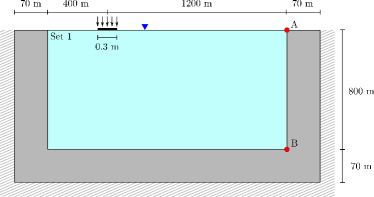
(a)

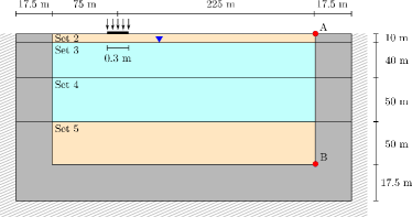
(b)

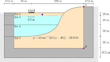
(c)

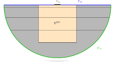
(d)

Figure 2: Poroelastic domains used for the numerical experiments in (a) homogeneous, (b) horizontally layered, and (c) horizontally layered with realistic interface to bedrock. The water table is marked with an inverted blue triangle. The red dots denote the locations where measurements of solid displacement ($\boldsymbol{u}$), fluid velocity ($\boldsymbol{w}$), and pressure ($p$) were taken. In Figure (d), a generic representation of the extended domains used in layered media is shown.

5 Numerical experiments

Three experiments were developed to evaluate the performance and accuracy of the proposed fully-mixed and hybrid PML formulations. The first experiment (referred as Experiment 1) considers a homogeneous poroelastic half-space where the water table is located at the free surface. In the second (Experiment 2), a three horizontally layered media over a half-space and water table below the second layer was considered (Figure 2b). The third (Experiment 3) adds a more realistic stratification including an outcropping (see Figure 2c). The material parameters used in the three cases are listed in Table 1. Set 1 corresponds approximately to a soft rock, while sets 2 to 5 represent standard soil parameters, from loose to dense sands.

Table 1: Material parameters, characteristic frequency of the medium, and wave propagation velocities of the porous media considered in the experiments. The set 1 was taken from Tables 1 and 2 in [16], whereas sets from 2 to 5 were defined by the authors to obtain soil-like wave velocities.

	Set 1	Set 2	Set 3	Set 4	Set 5
$\rho_{s}~{}(\text{kg}/\text{m}^{3})$	$2650$	$2600$	$2600$	$2600$	$2600$
$\rho_{f}~{}(\text{kg}/\text{m}^{3})$	$900$	$1.29$	$1000$	$1000$	$1.29$
$K_{s}~{}(\text{N}/\text{m}^{2})$	$12\times 10^{9}$	$2.3\times 10^{8}$	$2.3\times 10^{8}$	$2.5\times 10^{8}$	$4.6\times 10^{8}$
$K_{f}~{}(\text{N}/\text{m}^{2})$	$2\times 10^{9}$	$1.4\times 10^{5}$	$2\times 10^{9}$	$2\times 10^{9}$	$1.4\times 10^{5}$
$K_{b}~{}(\text{N}/\text{m}^{2})$	$10\times 10^{9}$	$1.5\times 10^{8}$	$1.5\times 10^{8}$	$1.7\times 10^{8}$	$4.2\times 10^{8}$
$\mu_{b}~{}(\text{N}/\text{m}^{2})$	$5\times 10^{9}$	$1.33\times 10^{8}$	$1.33\times 10^{8}$	$2.84\times 10^{8}$	$4.44\times 10^{8}$
$T$	$1.2$	$1$	$1$	$1$	$1$
$\kappa~{}(\text{m}^{2})$	$1\times 10^{-12}$	$8\times 10^{-9}$	$8\times 10^{-9}$	$1\times 10^{-10}$	$1\times 10^{-11}$
$\phi$	$0.3$	$0.2$	$0.2$	$0.2$	$0.2$
$\eta~{}(\text{Pa s})$	$1\times 10^{-3}$	$2\times 10^{-5}$	$1\times 10^{-3}$	$1\times 10^{-3}$	$2\times 10^{-5}$
$f_{c}~{}(\text{Hz})$	44210	62	4	318	49350
$c_{s}~{}(\text{m/s})$	960	300	300	400	500
$c_{1p}~{}(\text{m/s})$	2366	470	574	636	755
$c_{2p}~{}(\text{m/s})$	775	329	425	513	330
$f_{c}$: characteristic frequency of the medium, $c_{1p}$: fast primary wave velocity,
$c_{2p}$: slow primary wave velocity, $c_{s}$: shear wave velocity

To obtain a reference solution, we solved Biot’s equations given in (1) on an extended domain with dimensions large enough to avoid wave reflections at the exterior boundaries $\Omega^{\text{RD}}$. A zero displacement Dirichlet condition was imposed to both $\boldsymbol{u}$ and $\boldsymbol{w}$ in the exterior boundary $\Gamma_{D}$. A simulation time of 2.0 seconds (half of the runtime used for the PML experiments) was enough for comparison purposes in the extended domain simulations. For layered medium, the regular domain was embedded in the extended domain, and layers were extended to the exterior boundary (see Figure 2d). Additionally, a first-order paraxial boundary condition [1] was implemented to solve Biot’s equations also for comparison purposes. The PML domain shown in Figure 2 was removed for paraxial simulations and replaced by this ABC at this boundary.

A vertical load defined by a Ricker wavelet was applied on a $0.3~{}\text{m}$ width stripe of the free surface in the three experiments (see Figure 2a). The expression defining the source is as follows:

$$\boldsymbol{g}(t)=A\left[\begin{array}[]{c}0\\ S(t)\end{array}\right]\quad\text{with }S(t)=\frac{(0.25u^{2}-0.5)e^{-0.25u^{2}}-13e^{13.5}}{0.5+13e^{13.5}}\quad\text{and }0\leq t\leq\frac{6\sqrt{6}}{\omega_{r}}$$ (29)

where $A$ denotes the pulse amplitude and $u=\omega_{r}t-3\sqrt{6}$. In the previous expression, $\omega_{r}=2\pi f_{r}$ is the characteristic central angular frequency of the pulse. In all the experiments $A=10^{4}~{}\text{N/m}$ and $f_{r}=15~{}\text{Hz}$ were used. The frequency of this source was adjusted to obtain a frequency spectrum similar to those obtained from geophysical seismic surveys, which makes it suitable for the simulations.

The porous media utilized in the simulations exhibit primarily dispersive behavior, indicated by the characteristic frequency of the media ($f_{c}$) satisfying the inequality $f_{c}=(\eta\phi)/(2\pi\rho_{f}T\kappa)>f_{r}=15~{}\text{Hz}$, where the slowest primary wave does not propagate [9, 16]. Although the medium generated by the physical parameters in Set 3 (see Table 1) does not display dispersive behavior, its shear wave velocity is slower than its slowest volumetric wave. Therefore, the discretization parameters were chosen by considering only the fastest primary wave and the shear wave velocities for all media. The domain was discretized using triangular cells, and the element size ($\Delta x$) was adjusted to have a minimum of 12 elements per shortest wavelength, with the biggest possible element being chosen. In all simulations, elements in the vicinity of the surface load were refined to a size of $\Delta x=0.15~{}\text{m}$.

A third-order version of the scaling and attenuation profiles given in (8) (with $m=3$) was used for the simulations. The width of the PML, denoted by $L_{\text{PML}}$, was chosen to be ten times the element size once $\Delta x$ was fixed (see Table 1). The constant $\beta_{0}$ was calculated using the expression (9) with $R=10^{-4}$, while $\alpha_{0}$ was fixed at 5. For all the experiments considering M-PML stretching functions, $p^{(y/x)}$ and $p^{(x/y)}$ were used as $0.01$. A summary of the discretization and PML parameters is presented in Table 2.

The Newmark-$\beta$ method with $\beta=1/4$ and $\gamma=1/2$ (i.e., without numerical damping) was used for time discretization [34]. The time-step $\Delta t$ was calculated using the Courant-Friedrichs-Lewy criteria:

$$\Delta t<\text{CFL}\frac{\Delta x}{c_{1p}}$$ (30)

where $c_{1p}$ represents the velocity of the fast primary wave and $\text{CFL}=0.75$ is the Courant-Friedrichs-Lewy number.

Table 2: Element sizes and PML parameters used in the three experiments with homogeneous and layered media

	General parameters			PML parameters
Experiment	$\Delta x_{\text{global}}~{}\text{(m)}$	$\Delta x_{\text{source}}~{}\text{(m)}$	$\Delta t~{}\text{(s)}$	$R$	$L_{\text{PML}}~{}\text{(m)}$	$\alpha_{0}$
1	$7.8$	$0.15$	$10^{-3}$	$10^{-4}$	$78$	$5$
2 and 3	$1.4$	$0.15$	$10^{-3}$	$10^{-4}$	$14$	$5$
$\Delta x_{\text{global}}$: global element size; $\Delta x_{\text{local}}$: element size refinement near to external source
$\Delta t$: time step; $R$: reflection coefficient; $L_{\text{PML}}$: width of the PML layer

5.1 Metrics for performance evaluation

To evaluate the performance of the fully-mixed PML, hybrid PML, and paraxial methods, the poroelastic energy on $\Omega^{\text{RD}}$ was estimated and compared against the reference solution using the following expression:

$$E(t_{k}) =\frac{1}{2}\int_{\Omega^{\text{RD}}}\rho\dot{\boldsymbol{u}}(\boldsymbol{x},t_{k})\cdot\dot{\boldsymbol{u}}(\boldsymbol{x},t_{k})~{}d\Omega+\frac{1}{2}\int_{\Omega^{\text{RD}}}\rho C\mathbf{e}(\boldsymbol{u}(\boldsymbol{x},t_{k}),t_{k}):\mathbf{e}(\boldsymbol{u}(\boldsymbol{x},t_{k}),t_{k})~{}d\Omega$$

$$+\frac{1}{2}\int_{\Omega^{\text{RD}}}\rho_{w}\dot{\boldsymbol{w}}(\boldsymbol{x},t_{k})\cdot\dot{\boldsymbol{w}}(\boldsymbol{x},t_{k})~{}d\Omega+\frac{1}{2}\int_{\Omega^{\text{RD}}}\frac{1}{M}p(\boldsymbol{x},t_{k})\cdot p(\boldsymbol{x},t_{k})~{}d\Omega$$ (31)

$$+\int_{\Omega^{\text{RD}}}\rho_{f}\dot{\boldsymbol{u}}(\boldsymbol{x},t_{k})\cdot\dot{\boldsymbol{w}}(\boldsymbol{x},t_{k})~{}d\Omega$$

Finally, we obtained traces of $\boldsymbol{u}$, $\boldsymbol{w}$, and $p$ at different locations $\boldsymbol{x}_{i}$ in $\Omega^{\text{RD}}$ (see Figure 2). Normalized error metric are defined as:

$$e_{\boldsymbol{u}}(\boldsymbol{x}_{i},t_{k}) =\frac{\lVert\boldsymbol{u}_{\text{ref}}(\boldsymbol{x}_{i},t_{k})-\boldsymbol{u}(\boldsymbol{x}_{i},t_{k})\rVert_{2}}{\max_{t_{k}}\lVert\boldsymbol{u}_{\text{ref}}(\boldsymbol{x}_{i},t_{k})\rVert_{2}}$$ (32a)

$$e_{\boldsymbol{w}}(\boldsymbol{x}_{i},t_{k}) =\frac{\lVert\boldsymbol{w}_{\text{ref}}(\boldsymbol{x}_{i},t_{k})-\boldsymbol{w}(\boldsymbol{x}_{i},t_{k})\rVert_{2}}{\max_{t_{k}}\lVert\boldsymbol{w}_{\text{ref}}(\boldsymbol{x}_{i},t_{k})\rVert_{2}}$$ (32b)

$$e_{p}(\boldsymbol{x}_{i},t_{k}) =\frac{\lvert p_{\text{ref}}(\boldsymbol{x}_{i},t_{k})-p(\boldsymbol{x}_{i},t_{k})\rvert}{\max_{t_{k}}\lvert p_{\text{ref}}(\boldsymbol{x}_{i},t_{k})\rvert}$$ (32c)

where $\lvert\cdot\rvert$ is the absolute value and $\lVert\boldsymbol{f}\rVert_{2}=\sqrt{\sum_{i}f_{i}^{2}}$ the vector 2-norm. The sub-index $()_{\text{ref}}$ denotes the reference solution obtained in the extended domain simulations.

5.2 Implementation

All experiments were solved using the open-source computing platform FEniCS [2, 29]. To implement the hybrid PML problem, Multiphenics [6] was used as a complementary tool. The finite element meshes were generated using the Frontal-Delaunay algorithm in Gmsh [19]. Discretization of the displacements ($\boldsymbol{u}$ and $\boldsymbol{w}$) and pressures ($p$ and $\pi$) was carried out using continuous Lagrange polynomials of second and first order, respectively. The stress history $\mathbf{S}$ was discretized using discontinuous Lagrange polynomials of first order.

The Multifrontal Massively Parallel sparse direct Solver (MUMPS) and the Generalized Minimal Residual Method (GMRES) solvers were used to solve the linear systems obtained after assembling the discrete weak forms of the problems [4, 5, 3]. FEniCS is built with PETSc as linear algebra backend [4, 5, 3] and supports both solvers by default. The iterative solver was used only for the extended domain simulations with relative and absolute tolerances of $10^{-7}$ and $10^{-9}$, respectively [4]. To accelerate the convergence, the linear system of the extended domain simulation was right-preconditioned using the Parallel ILU preconditioner HYPRE-Euclid [23]. The direct solver was used with default parameters [2].

6 Results

In the upcoming sections, we will present and analyze energy graphs, traces, error traces, and snapshots of the propagating waves for all three experiments. Through these analyses, we aim to provide a comprehensive understanding of the simulations and their outcomes.

6.1 Experiment 1: homogeneous half-space

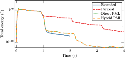
(a)

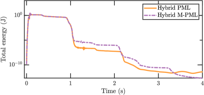
(b)

Figure 3: Energies estimated on $\Omega^{\text{RD}}$ using Equation (5.1) for the horizontally layered experiment. (a) Results show the extended, paraxial, fully-mixed, and hybrid PML results, and (b) a comparison between the hybrid PML and hybrid M-PML simulations. Both fully-mixed and hybrid formulations give identical results.

Figure 3a shows the poroelastic energy estimated using (5.1) for extended, paraxial, and PML simulations in a homogeneous half-space domain. The results demonstrate good agreement between the PML and reference solutions in the first 2 seconds of simulation time, although small differences are observed. The energy decay rate of the PML simulations is greater than that of the paraxial case, which consistently decays but a lower rate. The energy obtained from the hybrid and fully-mixed PML formulations showed no observable differences, indicating that both methods provide equivalent solutions (see Figure 3a). Additionally, the number of degrees of freedom (DOFs) in the hybrid case is approximately 1.7 times less than the fully-mixed problem (as shown in Table 3) because the tensor $\mathbf{S}$ does not need to be solved in $\Omega^{\text{RD}}$. Consequently, the hybrid formulation is significantly less computationally expensive than the fully-mixed form while maintaining the same properties.

Table 3: Number of degrees of freedom (DOFs) solved for extended, paraxial, fully-mixed PML, and hybrid PML formulations.

	Experiment 1	Experiment 2	Experiment 3
Extended	8,550,901	13,043,765	12,759,950
Paraxial	425,518	462,513	480,229
Fully-mixed PML	1,054,006	1,137,430	1,181,065
Hybrid PML	607,424	651,758	676,810

Figure 3b compares the energies obtained from the hybrid PML and M-PML formulations. During the first second of the simulation, the results are similar, and only small differences are observed. As the simulation progresses, the energy obtained with M-PML stretching functions is slightly larger than that obtained with uniaxial functions, indicating slightly worse performance. However, during the last second of simulation, the energy of the uniaxial case stops decaying showing even a slightly increase, while the energy of the M-PML case continues decaying. The reduced performance of M-PML (compared to PML) during the first seconds of simulation is because the stretching functions are not perfectly matched in $\Gamma_{I}$, generating spurious reflections. In fact, a M-PML absorbing layer can be interpreted as a sponge rather than a PML [31]. This is because the coupling of two damping directions causes the loss of the perfectly matched layer characteristic of Berenger’s technique [8]. Thus, the theoretical reflection coefficient for an infinite M-PML is not longer zero prior the discretization.

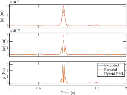
(a) A Point

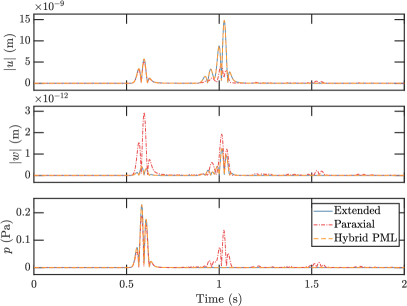
(b) B Point

Figure 4: Traces of $\boldsymbol{u}$, $\boldsymbol{w}$, and $p$ for Experiment 1 at the points highlighted in Figure 2a. Results obtained using the hybrid PML formulation show good agreement with the reference solution and no spurious reflections are observed.

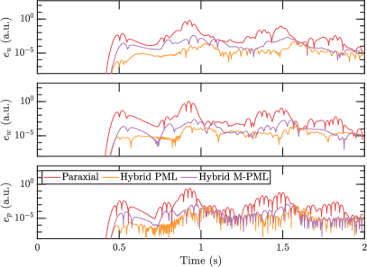
(a) Location A

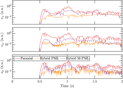
(b) Location B

Figure 5: Errors in the traces of $\boldsymbol{u}$, $\boldsymbol{w}$, and $p$ estimated using (32) for the Experiment 1 at the highlighted locations in Figure 2a. The vertical axis is logarithmic to facilitate visualization of differences. At the beginning of the simulation, all formulations yielded errors close to zero, which are omitted in the plot. As the simulation progressed, errors obtained using the hybrid PML and M-PML are smaller than those obtained using the paraxial case, although M-PML showed slightly worse performance between 0.5 and 1.5 s approximately because the stretching functions are not perfectly matched in this case. 3b.

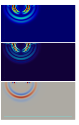
(a) $t=0.2$ s

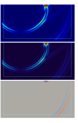
(b) $t=0.5$ s

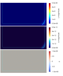
(c) $t=1$ s

Figure 6: Screenshots of the hybrid PML simulations at different time steps. The first row in the figure shows the solid displacement ($\boldsymbol{u}$), the second the relative fluid displacement ($\boldsymbol{w}$), and the third row the fluid pressure ($p$). No evident spurious reflections are observed at the interface between $\Omega^{\text{RD}}$ and $\Omega^{\text{PML}}$.

Traces of the solutions and errors calculated using (32) for the two locations shown in Figure 2a are presented in Figures 4 and 5. There is a good match between the hybrid PML and the extended domain simulations at both locations, in contrast to the paraxial case where reflections are observed. Looking at the errors, the superior performance of the hybrid PML method is evident, showing an improvement of at least three orders of magnitude compared to the paraxial case. In the same figure, the error obtained by using M-PML stretching functions in the hybrid simulation is depicted. As mentioned previously, results obtained using M-PML compared to PML are slightly worse between 0.5 and 1.5 s approximately because the stretching functions are not perfectly matched in this case. However, the results are still better than those obtained with the paraxial boundary conditions and more stable in time compared to the hybrid PML simulation (see Figure 3). Finally, screenshots of the solutions at different times can be found in Figure 6.

6.2 Experiment 2: horizontally-layered domain

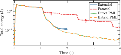
(a)

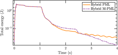
(b)

Figure 7: Energies estimated on $\Omega^{\text{RD}}$ using Equation (5.1) for the horizontally layered experiment. (a) Results show the extended, paraxial, fully-mixed, and hybrid PML results, and (b) a comparison between the hybrid PML and hybrid M-PML simulations. Both fully-mixed and hybrid formulations give identical results.

Figure 7a shows the poroelastic energies for extended, paraxial, and PML simulations in the horizontally-layered domain. Similarly, the results indicate good agreement between the PML and reference solutions within the first 2 seconds of simulation, although some small differences are observed. The energy decay rate of the PML simulations is greater than that of the paraxial case, which decays slowly but consistently. In this experiment, it is not evident from the plots that outgoing waves are reaching the boundaries of $\Omega^{\text{RD}}$, as the plateaus observed in Figure 3 are absent. This is due to reflections at the interfaces between layers (see Figures 2b and 10).

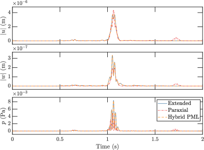
(a) Point A

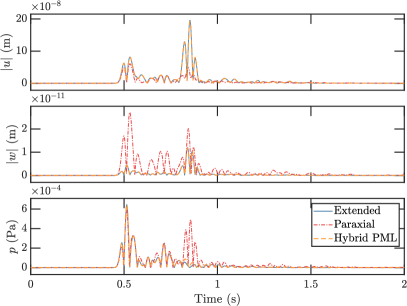
(b) Point B

Figure 8: Traces of $\boldsymbol{u}$, $\boldsymbol{w}$, and $p$ for the third experiment at the locations highlighted in Figure 2b. Results obtained using the hybrid PML formulation show good agreement with the extended domain solution.

The energies obtained using the hybrid and fully-mixed PML formulations produced almost the same results, illustrating that both methods provide similar solutions (see Figure 3a). Additionally, the number of DOFs in the hybrid case is approximately 1.8 times fewer than the fully-mixed problem (as shown in Table 3). Therefore, the hybrid formulation is less computationally expensive than the fully-mixed form while providing equivalent solutions. Regarding Figure 7b, in terms of decay rate, during the first 2.5 seconds of the simulation, the results obtained using PML and M-PML in the hybrid formulation are similar, and slightly greater errors are observed with M-PML between 1.5 and 2.5s. The worst performance of M-PML in this time window is because the stretching functions are not in perfectly matched at $\Gamma_{I}$, as mentioned in previous paragraphs, which generates spurious reflections [31]. However, during the last second, the energy of the uniaxial case decays more slowly than the M-PML case, which keeps a constant rate.

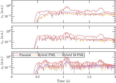
(a) Point A

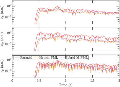
(b) Point B

Figure 9: Errors of the traces of $\boldsymbol{u}$, $\boldsymbol{w}$, and $p$ estimated using (32) for the Experiment 2 at the locations highlighted in Figure 2b. The vertical axis is in logarithmic scale to improve differences visualization. At the beginning of the simulation, errors obtained with both methods are close to zero and therefore are out from the vertical axis range. Results obtained with the hybrid PML formulation do not show observable differences compared to the reference solution.

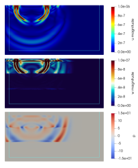
(a) $t=0.3$ s

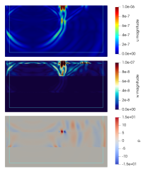
(b) $t=0.5$ s

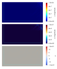
(c) $t=1.2$ s

Figure 10: Screenshots of the hybrid PML simulations at different time steps. The first row of the figure shows the solid displacement ($\boldsymbol{u}$), the second the relative fluid displacement ($\boldsymbol{w}$), and the third row the fluid pressure ($p$). No spurious reflections are observed at the interface between $\Omega^{\text{RD}}$ and $\Omega^{\text{PML}}$.

Figures 8 and 9 present traces of the solutions and errors calculated using (32) for two locations shown in Figure 2b. The results show a good match between the hybrid PML and extended domain simulations at both locations, in contrast to the paraxial case where reflections are observed. The error analysis confirms the marginally superior performance of the hybrid PML method with respect to the M-PML case, but shows a considerable improvement compared to the paraxial case. The difference between PML and M-PML results is due to imperfect matching of stretching functions in the last case. Nevertheless, the results obtained with M-PML are still superior to those obtained with paraxial boundary conditions and more stable over time than the hybrid PML simulation (see Figure 7).

Finally, Figure 10 presents screenshots that depict the propagation of waves at different times. These snapshots clearly show the transitions between different layers and the behavior of waves within each medium. For example, the layer with lower permeabilities (as shown in Table 1 and Figure 2b) exhibited smaller relative fluid displacements ($\boldsymbol{w}$) due to the small hydraulic conductivity. Additionally, media filled with air had lower pressures. Despite the complex behavior of waves in different media, the PML effectively absorbed and attenuated the waves during the simulation.

6.3 Experiment 3: layered domain with outcropping

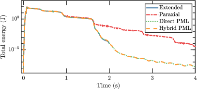
(a)

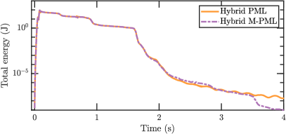
(b)

Figure 11: Energy estimated on $\Omega^{\text{RD}}$ using (5.1) for the Experiment 3. Results show the extended, paraxial, fully-mixed, and hybrid PML cases. Both fully-mixed and hybrid formulations give identical results.

As observed in the previous experiments, both hybrid and fully-mixed PML formulations produced superior results compared to the paraxial case. The energy plots for this experiment also shows an excellent agreement between the PML and reference solutions within the initial 2 seconds of simulation, with negligible differences, as illustrated in Figure 11a. Although the decay of energy was consistent over time in all methods, PML exhibited faster energy decay compared to the paraxial case. The energy plots indicate that the solutions obtained using the hybrid and fully-mixed PML formulations are almost indistinguishable, indicating that both methods produce nearly identical results. This observation is consistent with the results of the previous experiments. Additionally, the hybrid case had a reduction in the number of DOFs by almost 1.8 times compared to the fully-mixed case (as shown in Table 3).

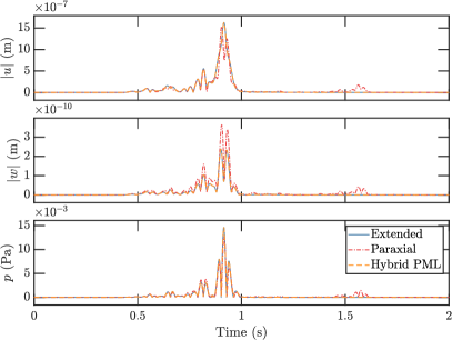
(a) Location A

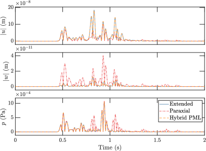
(b) Location B

Figure 12: Traces of $\boldsymbol{u}$, $\boldsymbol{w}$, and $p$ for the third experiment at the locations highlighted in Figure 2c. Results obtained using the hybrid PML formulation show good agreement with the reference solution.

Figure 11b compares the energies obtained using the hybrid PML and M-PML formulations. The results show that the two methods provide almost identical solutions up to seconds of the simulation, while some differences can be observed between 2 and 3 seconds, where PML slightly surpasses the multiaxial solution.. Interestingly, after 3 seconds of the simulation, the energy decay rate using M-PML is better with respect to the uniaxial case, highlighting the improved time-stability of M-PML stretching functions.

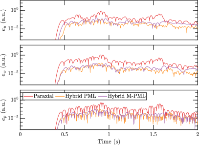
(a) Point A

(b) Point B

Figure 13: Errors of the traces of $\boldsymbol{u}$, $\boldsymbol{w}$, and $p$ estimated using (32) for the Experiment 3 at the locations highlighted in Figure 2c. Results obtained with the hybrid PML formulation do not show differences compared to the reference solution at Point A, while the paraxial approximation also performs reasonably well at this location.However, the advantages of the proposed method are much more evident at Point B.

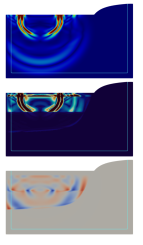
(a) $t=0.3$ s

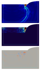
(b) $t=0.6$ s

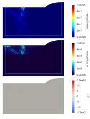
(c) $t=1.2$ s

Figure 14: Screenshots of the hybrid PML simulations at different time steps. The first row shows the solid displacement ($\boldsymbol{u}$), the second the relative fluid displacement ($\boldsymbol{w}$), and the third row the fluid pressure ($p$). No spurious reflections are observed at the interface between $\Omega^{\text{RD}}$ and $\Omega^{\text{PML}}$.

Traces of the solutions and their corresponding errors, calculated using (32), for the two locations illustrated in Figure 2c, are presented in Figures 12 and 13, respectively. These figures confirm the excellent agreement between the hybrid PML and the extended domain simulation at both locations, with no observable reflections unlike the paraxial case. The error analysis shows a considerable improvement compared to the paraxial case and slightly superior performance of the hybrid PML method with respect to the M-PML case. However, it is worth noting that the results obtained with M-PML are still better than those obtained with paraxial boundary conditions and exhibit better stability over time than the hybrid PML simulation.

Figure 14 shows snapshots of the solutions at different times. Due to the complex interfaces between materials in the medium, the waves interact in intricate ways generating complex patterns of reflected waves at interfaces as can be seen in the figure. Despite this complexity, the PML effectively absorbed the waves at the boundary of $\Omega^{\text{RD}}$, and no unwanted reflections were observed.

7 Conclusions

We proposed fully-mixed and hybrid formulations of the PML method for the simulation of poroelastic waves in truncated domains. Compared to other methods, both introduce only three additional scalar unknowns, i.e., the components of the symmetric stress-history tensor, reducing the number of unknowns with respect to current split- and unsplit-field formulations. However, the hybrid formulation considerably reduced the degrees of freedom required to solve the propagation problem when compared to the fully-mixed and extended domain simulations, because new unknowns are only defined in the boundary layer. On average, the hybrid PML formulation reduced the number of DOFs by approximately 1.8 times compared to the fully-mixed form and by 18 times compared to the extended domain simulations. However, in comparison to the paraxial case, the hybrid PML formulation increased the number of DOFs by almost 41%. However, although effective for some applications, paraxial boundary conditions are not ideal for absorbing surface waves. Therefore, they are not recommended in problems where surface waves are predominant.

The proposed formulations of the PML method are prone to the same issues of other PML formulations, and they may suffer instability over time under certain circumstances. However, a significant advantage of the proposed methods is that they enable the scaling and attenuation functions to be redefined using stretching functions with superior absorbing properties, such as M-PML, without modifying the underlying partial differential equations. Moreover, the time-integration scheme used for the simulations did not consider numerical damping, making the problem conditions even more demanding compared to other methods [21, 22]. Only small time instabilities were observed, and they were fixed using M-PML.

In terms of discretization, the element size was selected as large as possible to reduce the number of DOFs. Additionally, only P2-P2-P1 finite element triplets were utilized to represent the solutions to the problems. This approach considerably reduced the computational effort required to solve the problem, unlike in previous studies. As a result, the hybrid and fully-mixed PML formulations proposed in this article have demonstrated robustness for demanding discretization and physical media conditions.

The following steps regarding this investigation are: (1) to extend fully-mixed and hybrid formulations to the 3D case to simulate more realistic scenarios for exmaple for complex seismic geophysical applications. (2) To consider variable and discontinuous porosities in space which would introduce discontinuities in the relative fluid displacement. (3) To apply the 2D and 3D formulations to solve inverse problems in porous media. And (4), to simulate and understand the propagation of poroelastic waves in the human body, which is particularly interesting in the fields of Magnetic Resonance Imaging and Ultrasound and is closely related to the elastography problem [14, 25].

8 Acknowledgments

HM and JM acknowledge the financial support given by ANID through the projects ANID-FONDECYT Postdoctorado #3220266 and ANID-FONDECYT Regular #1230864, respectively. ES was partially funded by a grant from the Research Center for Integrated Disaster Risk Management CIGIDEN Project 1522A0005 FONDAP 2022.

References

- Akiyoshi et al. [1994] Akiyoshi, T., Fuchida, K., Fang, H.L., 1994. Absorbing boundary conditions for dynamic analysis of fluid-saturated porous media. Soil Dynamics and Earthquake Engineering 13, 387–397. doi:10.1016/0267-7261(94)90009-4.
- Alnaes et al. [2015] Alnaes, M.S., Blechta, J., Hake, J., Johansson, A., Kehlet, B., Logg, A., Richardson, C., Ring, J., Rognes, M.E., Wells, G.N., 2015. The FEniCS Project Version 1.5. Archive of Numerical Software 3, 9–23. URL: http://journals.ub.uni-heidelberg.de/index.php/ans/article/view/20553, doi:10.11588/ans.2015.100.20553.
- Balay et al. [2020a] Balay, S., Abhyankar, S., Adams, M.F., Brown, J., Brune, P., Buschelman, K., Dalcin, L., Dener, A., Eijkhout, V., Gropp, W.D., Kaushik, D., Knepley, M.G., May, D.A., McInnes, L.C., Mills, R.T., Munson, T., Rupp, K., Sanan, P., Smith, B.F., Zampini, S., Zhang, H., Zhang, H., 2020a. PETSc Users Manual. Technical Report ANL-95/11 - Revision 3.13. Argonne National Laboratory.
- Balay et al. [2020b] Balay, S., Abhyankar, S., Adams, M.F., Brown, J., Brune, P., Buschelman, K., Dalcin, L., Dener, A., Eijkhout, V., Gropp, W.D., Kaushik, D., Knepley, M.G., May, D.A., McInnes, L.C., Mills, R.T., Munson, T., Rupp, K., Sanan, P., Smith, B.F., Zampini, S., Zhang, H., Zhang, H., 2020b. PETSc Web page. Https://www.mcs.anl.gov/petsc.
- Balay et al. [1997] Balay, S., Gropp, W.D., McInnes, L.C., Smith, B.F., 1997. Efficient management of parallelism in object oriented numerical software libraries, in: Arge, E., Bruaset, A.M., Langtangen, H.P. (Eds.), Modern Software Tools in Scientific Computing, Birkhauser Press. pp. 163–202.
- Ballarin [2016] Ballarin, F., 2016. Multiphenics - Easy Prototyping of Multiphysics Problems in FEniCS. https://mathlab.sissa.it/multiphenics. Accessed: 2023-01-04.
- Basu and Chopra [2004] Basu, U., Chopra, A.K., 2004. Perfectly matched layers for transient elastodynamics of unbounded domains. International Journal for Numerical Methods in Engineering 59, 1039–1074. URL: https://onlinelibrary.wiley.com/doi/abs/10.1002/nme.896, doi:10.1002/nme.896. _eprint: https://onlinelibrary.wiley.com/doi/pdf/10.1002/nme.896.
- Berenger [1994] Berenger, J.P., 1994. A perfectly matched layer for the absorption of electromagnetic waves. Journal of Computational Physics 114, 185–200. doi:10.1006/jcph.1994.1159.
- Biot [1956] Biot, M.A., 1956. Theory of Propagation of Elastic Waves in a Fluid‐Saturated Porous Solid. I. Low‐Frequency Range. The Journal of the Acoustical Society of America 28, 168–178. URL: https://asa.scitation.org/doi/10.1121/1.1908239, doi:10.1121/1.1908239. publisher: Acoustical Society of America.
- Biot [1962] Biot, M.A., 1962. Generalized Theory of Acoustic Propagation in Porous Dissipative Media. The Journal of the Acoustical Society of America 34, 1254–1264. doi:10.1121/1.1918315.
- Chew and Liu [1996] Chew, W., Liu, Q., 1996. Perfectly matched layers for elastodynamics: a new absorbing boundary condition. Journal of Computational Acoustics 04, 341–359. URL: https://www.worldscientific.com/doi/abs/10.1142/S0218396X96000118, doi:10.1142/S0218396X96000118. publisher: World Scientific Publishing Co.
- Collino and Tsogka [2001] Collino, F., Tsogka, C., 2001. Application of the perfectly matched absorbing layer model to the linear elastodynamic problem in anisotropic heterogeneous media. Geophysics 66, 294–307. URL: https://doi.org/10.1190/1.1444908, doi:10.1190/1.1444908.
- Correia and Jian-Ming Jin [2005] Correia, D., Jian-Ming Jin, 2005. On the development of a higher-order PML. IEEE Transactions on Antennas and Propagation 53, 4157–4163. URL: http://ieeexplore.ieee.org/document/1549999/, doi:10.1109/TAP.2005.859901.
- Doyley [2012] Doyley, M.M., 2012. Model-based elastography: a survey of approaches to the inverse elasticity problem. Physics in Medicine & Biology 57, R35. URL: https://dx.doi.org/10.1088/0031-9155/57/3/R35, doi:10.1088/0031-9155/57/3/R35. publisher: IOP Publishing.
- Drossaert and Giannopoulos [2007] Drossaert, F.H., Giannopoulos, A., 2007. Complex frequency shifted convolution PML for FDTD modelling of elastic waves. Wave Motion 44, 593–604. doi:10.1016/J.WAVEMOTI.2007.03.003. publisher: Elsevier.
- Dudley Ward et al. [2017] Dudley Ward, N.F., Lähivaara, T., Eveson, S., 2017. A discontinuous Galerkin method for poroelastic wave propagation: The two-dimensional case. Journal of Computational Physics 350, 690–727. URL: http://dx.doi.org/10.1016/j.jcp.2017.08.070, doi:10.1016/j.jcp.2017.08.070. publisher: Elsevier Inc.
- Ezziani [2005] Ezziani, A., 2005. Modélisation mathématique et numérique de la propagation d’ondes dans les milieux viscoélastiques et poroélastiques. These de doctorat. Paris 9. URL: https://www.theses.fr/2005PA090019.
- François et al. [2021] François, S., Goh, H., Kallivokas, L.F., 2021. Non-convolutional second-order complex-frequency-shifted perfectly matched layers for transient elastic wave propagation. Computer Methods in Applied Mechanics and Engineering 377, 113704. URL: https://linkinghub.elsevier.com/retrieve/pii/S0045782521000402, doi:10.1016/j.cma.2021.113704. publisher: North-Holland.
- Geuzaine and Remacle [2009] Geuzaine, C., Remacle, J.F., 2009. Gmsh: A 3-D finite element mesh generator with built-in pre- and post-processing facilities. International Journal for Numerical Methods in Engineering 79, 1309–1331. URL: https://onlinelibrary.wiley.com/doi/abs/10.1002/nme.2579, doi:10.1002/nme.2579. _eprint: https://onlinelibrary.wiley.com/doi/pdf/10.1002/nme.2579.
- Gwinner and Stephan [2018] Gwinner, J., Stephan, E., 2018. Advanced Boundary Element Methods: Treatment of Boundary Value, Transmission and Contact Problems. Springer Series in Computational Mathematics, Springer International Publishing. URL: https://link.springer.com/book/10.1007/978-3-319-92001-6.
- He et al. [2019a] He, Y., Chen, T., Gao, J., 2019a. Perfectly matched absorbing layer for modelling transient wave propagation in heterogeneous poroelastic media. Journal of Geophysics and Engineering URL: https://academic.oup.com/jge/advance-article/doi/10.1093/jge/gxz080/5603739, doi:10.1093/jge/gxz080.
- He et al. [2019b] He, Y., Chen, T., Gao, J., 2019b. Unsplit perfectly matched layer absorbing boundary conditions for second-order poroelastic wave equations. Wave Motion 89, 116–130. URL: https://doi.org/10.1016/j.wavemoti.2019.01.004, doi:10.1016/j.wavemoti.2019.01.004.
- Hysom and Pothen [2001] Hysom, D., Pothen, A., 2001. A Scalable Parallel Algorithm for Incomplete Factor Preconditioning. SIAM Journal on Scientific Computing 22, 2194–2215. URL: https://epubs.siam.org/doi/10.1137/S1064827500376193, doi:10.1137/S1064827500376193. publisher: Society for Industrial and Applied Mathematics.
- Kausel [1988] Kausel, E., 1988. Local Transmitting Boundaries. Journal of Engineering Mechanics 114, 1011–1027. URL: https://ascelibrary.org/doi/abs/10.1061/%28ASCE%290733-9399%281988%29114%3A6%281011%29, doi:10.1061/(ASCE)0733-9399(1988)114:6(1011). publisher: American Society of Civil Engineers.
- Kolipaka et al. [2009] Kolipaka, A., McGee, K.P., Manduca, A., Romano, A.J., Glaser, K.J., Araoz, P.A., Ehman, R.L., 2009. Magnetic resonance elastography: Inversions in bounded media. Magnetic Resonance in Medicine 62, 1533–1542. URL: http://doi.wiley.com/10.1002/mrm.22144, doi:10.1002/mrm.22144. publisher: Wiley-Blackwell.
- Kucukcoban and Kallivokas [2011] Kucukcoban, S., Kallivokas, L.F., 2011. Mixed perfectly matched layers for direct transient analysis in 2D elastic heterogeneous media. Comput. Meth. Appl. Mech. Eng. 200, 57–76.
- Kucukcoban and Kallivokas [2013] Kucukcoban, S., Kallivokas, L.F., 2013. A symmetric hybrid formulation for transient wave simulations in PML-truncated heterogeneous media. Wave Motion 50, 57–79. doi:10.1016/j.wavemoti.2012.06.004.
- Kuzuoglu and Mittra [1996] Kuzuoglu, M., Mittra, R., 1996. Frequency dependence of the constitutive parameters of causal perfectly matched anisotropic absorbers. IEEE Microwave and Guided Wave Letters 6, 447–449. URL: http://ieeexplore.ieee.org/document/544545/, doi:10.1109/75.544545.
- Logg et al. [2012] Logg, A., Mardal, K.A., Wells, G. (Eds.), 2012. Automated Solution of Differential Equations by the Finite Element Method. volume 84 of Lecture Notes in Computational Science and Engineering. Springer, Berlin, Heidelberg. URL: http://link.springer.com/10.1007/978-3-642-23099-8, doi:10.1007/978-3-642-23099-8.
- [30] Martin, R., Komatitsch, D., Ezziani, A., . An unsplit convolutional perfectly matched layer improved at grazing incidence for seismic wave propagation in poroelastic media. Geophysics 73, T51–T61. URL: https://library.seg.org/doi/abs/10.1190/1.2939484, doi:10.1190/1.2939484. publisher: Society of Exploration Geophysicists.
- Martin et al. [2010] Martin, R., Komatitsch, D., Gedney, S., Bruthiaux, E., 2010. A High-Order Time and Space Formulation of the Unsplit Perfectly Matched Layer for the Seismic Wave Equation Using Auxiliary Differential Equations (ADE-PML). Computer Modeling in Engineering & Sciences 56, 17–42. URL: https://www.techscience.com/CMES/v56n1/25463, doi:10.3970/cmes.2010.056.017. publisher: Tech Science Press.
- Meza-Fajardo and Papageorgiou [2008] Meza-Fajardo, K.C., Papageorgiou, A.S., 2008. A Nonconvolutional, Split-Field, Perfectly Matched Layer for Wave Propagation in Isotropic and Anisotropic Elastic Media: Stability Analysis. Bulletin of the Seismological Society of America 98, 1811–1836. URL: https://doi.org/10.1785/0120070223, doi:10.1785/0120070223.
- Morency and Tromp [2008] Morency, C., Tromp, J., 2008. Spectral-element simulations of wave propagation in porous media. Geophysical Journal International 175, 301–345. doi:10.1111/j.1365-246X.2008.03907.x.
- Newmark [1959] Newmark, N.M., 1959. A Method of Computation for Structural Dynamics. Journal of the Engineering Mechanics Division 85, 67–94. URL: https://ascelibrary.org/doi/10.1061/JMCEA3.0000098, doi:10.1061/JMCEA3.0000098. publisher: American Society of Civil Engineers.
- Qi and Geers [1998] Qi, Q., Geers, T.L., 1998. Evaluation of the Perfectly Matched Layer for Computational Acoustics. Journal of Computational Physics 139, 166–183. doi:10.1006/jcph.1997.5868.
- Song et al. [2005] Song, R., Ma, J., Wang, K., 2005. The application of the nonsplitting perfectly matched layer in numerical modeling of wave propagation in poroelastic media. Applied Geophysics 2, 216–222. URL: https://doi.org/10.1007/s11770-005-0027-3, doi:10.1007/s11770-005-0027-3.
- Wang and Tang [2003] Wang, T., Tang, X., 2003. Finite-difference modeling of elastic wave propagation: A nonsplitting perfectly matched layer approach. Geophysics 68, 1749–1755. doi:10.1190/1.1620648.
- Zeng et al. [2001] Zeng, Y.Q., He, J.Q., Liu, Q.H., 2001. The application of the perfectly matched layer in numerical modeling of wave propagation in poroelastic media. Geophysics 66, 1258–1266. URL: http://library.seg.org/doi/10.1190/1.1487073, doi:10.1190/1.1487073. iSBN: 0016-8033.
- [39] Zeng, Y.Q., Liu, Q.H., . A staggered-grid finite-difference method with perfectly matched layers for poroelastic wave equations. The Journal of the Acoustical Society of America 109, 2571–2580. URL: https://doi.org/10.1121/1.1369783, doi:10.1121/1.1369783.
- Zhou et al. [2016] Zhou, F.X., Ma, Q., Gao, B.B., 2016. Efficient unsplit perfectly matched layers for finite-element time-domain modeling of elastodynamics. Journal of Engineering Mechanics 142, 1–12. doi:10.1061/(ASCE)EM.1943-7889.0001145.
- Zienkiewicz et al. [1980] Zienkiewicz, O.C., Chang, C.T., Bettess, P., 1980. Drained, undrained, consolidating and dynamic behaviour assumptions in soils. Géotechnique 30, 385–395. URL: http://www.icevirtuallibrary.com/doi/10.1680/geot.1980.30.4.385, doi:10.1680/geot.1980.30.4.385. publisher: Thomas Telford Ltd.
- Zienkiewicz and Shiomi [1984] Zienkiewicz, O.C., Shiomi, T., 1984. Dynamic behaviour of saturated porous media; The generalized Biot formulation and its numerical solution. International Journal for Numerical and Analytical Methods in Geomechanics 8, 71–96. URL: https://onlinelibrary.wiley.com/doi/full/10.1002/nag.1610080106, doi:10.1002/NAG.1610080106. publisher: John Wiley & Sons, Ltd.