Average partial effect estimation using double machine learning

Abstract

Single-parameter summaries of variable effects are desirable for ease of interpretation, but linear models, which would deliver these, may fit poorly to the data. A modern approach is to estimate the average partial effect—the average slope of the regression function with respect to the predictor of interest—using a doubly robust semiparametric procedure. Most existing work has focused on specific forms of nuisance function estimators. We extend the scope to arbitrary plug-in nuisance function estimation, allowing for the use of modern machine learning methods which in particular may deliver non-differentiable regression function estimates. Our procedure involves resmoothing a user-chosen first-stage regression estimator to produce a differentiable version, and modelling the conditional distribution of the predictors through a location–scale model. We show that our proposals lead to a semiparametric efficient estimator under relatively weak assumptions. Our theory makes use of a new result on the sub-Gaussianity of Lipschitz score functions that may be of independent interest. We demonstrate the attractive numerical performance of our approach in a variety of settings including ones with misspecification.

1 Introduction

A common goal of practical data analysis is to quantify the effect that a particular predictor or set of predictors $X$ has on a response $Y$, whilst accounting for the contribution of a vector of other predictors $Z$. Single-parameter summaries are often desirable for ease-of-interpretability, as demonstrated by the popularity of (partially) linear models. Such models, however, may not adequately capture the conditional mean of the response, potentially invalidating conclusions drawn. Indeed the successes of model-agnostic regression methods such as XGBoost [Chen and Guestrin, 2016], random forests [Breiman, 2001] and deep learning [Goodfellow et al., 2016] in machine learning competitions such as those hosted by Kaggle [Bojer and Meldgaard, 2021] suggest that such models fitting poorly is to be expected in many contemporary datasets of interest.

When $X\in\mathbb{R}$ is a continuous random variable and the conditional mean $f(x,z):=\mathbb{E}(Y\,|\,X=x,Z=z)$ is differentiable in the $x$-direction, a natural quantity of interest is the average slope with respect to $x$, holding $Z$ constant. This is known as the average partial effect (or average derivative), defined as

$$\theta:=\mathbb{E}\bigg{[}\frac{\partial}{\partial x}f(X,Z)\bigg{]}.$$

This has historically been considered for estimation of linear coefficients in index models [Stoker, 1986, Powell et al., 1989], but may be thought of more generally as the average effect of incrementing the value of $X$ by an infinitesimal amount, holding $Z$ constant. It is also the average slope of the so-called partial dependence plot, popular in the field of interpretable machine learning [Friedman, 2001, Zhao and Hastie, 2021, Molnar, 2022].

Rothenhäusler and Yu [2020] provide a causal interpretation of this quantity in the form of an average outcome change if the ‘treatment’ $X$ of all subjects were changed by an arbitrarily small quantity. In this sense, $\theta$ may be thought of as a continuous analogue of the well-studied average treatment effect functional $\mathbb{E}\{\mathbb{E}(Y\,|\,Z,X=1)-\mathbb{E}(Y\,|\,Z,X=0)\}=\mathbb{E}\{f(1,Z)-f(0,Z)\}$ in the case where $X$ is discrete, only taking values $0$ or $1$ [Robins et al., 1994, Robins and Rotnitzky, 1995, Scharfstein et al., 1999a].

Note also that in the partially linear model

$$f(x,z)=\theta x+g(z),$$

the average partial effect reduces to the linear coefficient. Thus the average partial effect may be thought of as a generalisation of the coefficient in a partially linear model that appropriately measures the association of $X$ and the response, while controlling for $Z$, even when there may be complex interactions between $X$ and $Z$ present.

While the average partial effect is easy to interpret, estimating the derivative of a conditional mean function is challenging. Regression estimators for $f$ which have been trained to have good mean-squared prediction error can produce arbitrarily bad derivative estimates, if they are capable of returning these at all. For example, highly popular tree-based methods give piecewise constant estimated regression functions and so clearly provide unusable estimates for the derivative of $f$.

Moreover, even if the rate of convergence of the derivative estimates was comparable to the mean-squared prediction error when estimating $f$ nonparametrically, an estimator of $\theta$ formed through their empirical average would typically suffer from plug-in bias and fail to attain the parametric rate of convergence. As well as poor estimation quality, this would also make inference, that is, performing hypothesis tests or forming confidence intervals, particularly problematic. The rich theory of semiparametric statistics [Bickel et al., 1993, Tsiatis, 2006] addresses the issue of such plug-in biases more generally, and supports the construction of debiased estimators based on (efficient) influence functions. This basic approach forms a cornerstone of what has become known as debiased or double machine learning: a collection of methodologies involving user-chosen machine learning methods to produce estimates of nuisance parameters that are used in the construction of estimators of functionals that enjoy parametric rates of convergence (see for example the review article Kennedy [2022] and references therein).

Procedurally, this often involves modelling both the conditional expectation $f$ and a function of the joint distribution of the predictors $(X,Z)$, with the bias of the overall estimator controlled by a product of biases relating to each of these models [Rotnitzky et al., 2021]. For the average partial effect, as shown by Powell et al. [1989], Newey and Stoker [1993], the predictor-based quantity to be estimated is the so-called score function (sometimes termed the negative score function)

$$\rho(x,z) :=\frac{\frac{\partial}{\partial x}p(x\mid z)}{p(x\mid z)}=\frac{\partial}{\partial x}\log p(x\mid z),$$

where $p(x\mid z)$ is the (assumed differentiable) conditional density of $X$ given $Z$. This has been studied in the unconditional setting (i.e. without any $Z$ present) using estimators based on parametric families [Stoker, 1986], splines [Cox, 1985, Ng, 1994, Bera and Ng, 1995], kernel smoothing methods [Härdle and Stoker, 1989, Powell et al., 1989, Stoker, 1990, Li, 1996], and reproducing kernel Hilbert spaces [Sriperumbudur et al., 2017].

Nonparametric estimation in the multivariate setting is extremely challenging owing to the complex nature of potential interactions and the stability issues related to dividing by estimated conditional densities. One approach to tackling this issue is to assume that the regression function $f$ and its derivative are sufficiently well-approximated by sparse linear combinations of basis functions [Rothenhäusler and Yu, 2020, Chernozhukov et al., 2022d]. Similarly to the case with the debiased Lasso [Zhang and Zhang, 2014] where regression coefficients can be estimated without placing explicit sparsity assumptions relating to the conditional distribution of $X$ given $Z$ (see for example Shah and Bühlmann [2023]); in this case, fewer assumptions need to be placed on the estimator of $\rho$ Chernozhukov et al. [2022d, Remark 4.1]. A related approach relies on $\rho$ itself being well-approximated by a sparse linear combination of basis functions; see Chernozhukov et al. [2022a, 2020, c, d, 2021, 2023] for examples of both of these approaches. In practice however, it may not always be clear what set of basis functions to choose. Chernozhukov et al. [2022b] adapts deep learning architectures and tree splitting criteria to develop neural network and random forest-based approaches for estimating $\rho$.

An alternative approach is to consider the estimated score function evaluated at the data points to be a set of weights to be chosen. Hirshberg and Wager [2021] assume that the regression estimation error lies within some absolutely convex class of functions, and perform a convex optimisation to choose weights that minimise the worst-case mean-squared error over this class. A version of this for single index-models is considered in Hirshberg and Wager [2020].

1.1 Our contributions and organisation of the paper

In this paper we develop new approaches for addressing the two main challenges in estimating the average partial effect $\theta$ using a double machine learning framework as outlined above, namely estimation of the derivative of the conditional mean function and conditional score estimation.

In Section 2 we first give a uniform asymptotic convergence result for such doubly robust estimators of $\theta$ requiring user-chosen estimators for $f$ and $\rho$. We argue that uniform results as opposed to pointwise results are particularly important in nonparametric settings such as those considered here. Indeed, considering the problem of testing for a non-zero partial effect, one can show that this is fundamentally hard: when $Z$ is a continuous random variable, any test must have power at most its size. This comes as a consequence of noting that the null in question contains the null that $X\mbox{${}\perp\mkern-11.0mu\perp{}$}Y\,|\,Z$, which is known to suffer from this form of impossibility [Shah and Peters, 2020, Thm. 2]. This intrinsic hardness means that any non-trivial test must restrict the null further with the form of these additional conditions, which would be revealed in a uniform result but may be absent in a pointwise analysis, providing crucial guidance on the suitability of tests in different practical settings.

In our case, the conditions for our result involve required rates of convergence for estimation of the conditional mean $f$, the score $\rho$ and also a condition on the quality of our implied estimate of the derivative of $f$. While estimation of conditional means is a task statisticians are familiar with tackling using machine learning methods for example, the latter two remain challenging to achieve. In contrast to existing work, rather than relying on well-chosen basis function expansions or developing bespoke estimation tools we aim to leverage once again the predictive ability of modern machine learning methods, which have a proven track record of success in practice.

For derivative estimation, we propose a post-hoc kernel smoothing procedure on top of the chosen regression method for estimating $f$. Importantly then we do not require any specific assumptions on complexity or stability properties of the estimator of $f$, or mean-square continuity [Chernozhukov et al., 2022d]. In Section 3 we show that under mild conditions, our resmoothing method achieves consistent derivative estimation (in terms of mean-square error) at no asymptotic cost to estimation of $f$ when comparing to the convergence rate enjoyed by the original regression method.

Turning to score estimation, we seek to reduce the problem of conditional score estimation to that of unconditional score estimation, which is much better studied [Cox, 1985, Ng, 1994, Bera and Ng, 1995]. In Section 4 we advocate modelling the conditional distribution of $X\mid Z$ as a location–scale model (see for example Kennedy et al. [2017, Sec. 5] who work with this in an application requiring conditional density estimation),

$$X=m(Z)+\sigma(Z)\varepsilon,$$

where $\varepsilon$ is mean-zero and independent of $Z$. Through estimating the conditional mean $m$ and $\sigma$ via some $\hat{m}$ and $\hat{\sigma}$, one can form scaled residuals $\{X-\hat{m}(Z)\}/\hat{\sigma}(Z)$ which may be fed to an unconditional score estimator. Theoretically, we consider settings where $\varepsilon$ is sub-Gaussian and $\sigma$ is nonparametric, and also the case where $\varepsilon$ is allowed to be heavy-tailed and $\sigma=1$ (i.e. a location only model where the errors $X-m(Z)\mbox{${}\perp\mkern-11.0mu\perp{}$}X$). We also demonstrate good numerical performance in heterogeneous, heavy-tailed settings. Given how even the unconditional score involves a division by a density, one concern might be that any errors in estimating $m$ and $\sigma$ may propagate unfavourably to estimation of the score. We show however that the estimation error for the multivariate $\rho(x,z)$ may be bounded by the sum of the estimation errors for the conditional mean $m$, the conditional scale $\sigma$ and the unconditional score function for the residual $\varepsilon$ alone. In this way we reduce the problem of conditional score estimation to unconditional score estimation, plus regression and heterogeneous scale estimation, all of which may be relatively more straightforward. Our results rely on proving a sub-Gaussianity property of Lipschitz score functions, which may be of independent interest.

Numerical comparisons of our methodology to existing approaches are contained in Section 5, where we demonstrate in particular that the coverage properties of confidence intervals based on our estimator have favourable coverage over a range of settings, both where our theoretical assumptions are met and where they are not satisfied. We conclude with a discussion in Section 6. Proofs and additional results are relegated to the appendix. We provide an implementation of our methods in the R package drape (Doubly Robust Average Partial Effects) available from https://github.com/harveyklyne/drape.

1.2 Notation

Let $(Y,X,Z)$ be a random triple taking values in $\mathbb{R}\times\mathbb{R}^{d}\times\mathcal{Z}$, where $\mathcal{Z}$ may be a mixture of discrete and continuous space. In order to present results that are uniform over a class of distributions $P$ for $(Y,X,Z)$, we will often subscript associated quantities by $P$. For example when $(Y,X,Z)\sim P$, we denote by $\mathbb{P}_{P}((Y,X,Z)\in A)$, the probability that $(Y,X,Z)$ lies in a (measurable) set $A$, and write $f_{P}(x,z):=\mathbb{E}_{P}(Y\mid X=x,Z=z)$ for the conditional mean function.

Let $\mathcal{P}_{0}$ be the set of distributions $P$ for $(Y,X,Z)$ where both $f_{P}$ and the conditional density of the predictors (with respect to the Lebesgue measure) $p_{P}(x\mid z)$ exist and are differentiable over all of $\mathbb{R}^{d}$, for almost every $z\in\mathcal{Z}$.

Write $\nabla$ for the $d$-dimensional differentiation operator with respect to the $x$, which we replace with ^′ if we are enforcing the case $d=1$. For each $P\in\mathcal{P}_{0}$, define the score function $\rho_{P}(x,z):=\nabla\log p_{P}(x\mid z)$, where $p_{P}(x\mid z)$ is the conditional probability density of $X\mid\{Z=z\}$ according to $P$. Note that $\rho_{P}$ exists for each $P\in\mathcal{P}_{0}$ and almost every $(X,Z)$, taking values in $\mathbb{R}^{d}$. Denote by $\Phi$ the standard $d$-dimensional normal cumulative distribution function (c.d.f.), and understand inequalities between vectors to apply elementwise.

We will sometimes introduce standard Gaussian random variables $W\sim N(0,1)$ independent of $(X,Z)$. Recall that a random variable $X\in\mathbb{R}$ is sub-Gaussian with parameter $\sigma$ if it satisfies $\mathbb{E}[\exp(\lambda X)]\leq\exp(\lambda^{2}\sigma^{2}/2)$ for all $\lambda\in\mathbb{R}$. A vector $V\in\mathbb{R}^{d}$ is sub-Gaussian with parameter $\sigma$ if $u^{T}V$ is sub-Gaussian with parameter $\sigma$ for any $u\in\mathbb{R}^{d}$ satisfying $\|u\|_{2}=1$.

As in Rask Lundborg et al. [2022], given a family of sequences of real-valued random variables $(W_{P,n})_{P\in\mathcal{P},n\in\mathbb{N}}$ taking values in a finite-dimensional vector space and whose distributions are determined by $P\in\mathcal{P}$, we write $W_{P,n}=o_{\mathcal{P}}(1)$ if $\sup_{P\in\mathcal{P}}\mathbb{P}_{P}(|W_{P,n}|>\epsilon)\to 0$ for every $\epsilon>0$. Similarly, we write $W_{P,n}=O_{\mathcal{P}}(1)$ if, for any $\epsilon>0$, there exist $M_{\epsilon},N_{\epsilon}>0$ such that $\sup_{n\geq N_{\epsilon}}\sup_{P\in\mathcal{P}}\mathbb{P}_{P}(|W_{P,n}|>M_{\epsilon})<\epsilon$. Given a second family of sequences of random variables $(V_{P,n})_{P\in\mathcal{P},n\in\mathbb{N}}$, we write $W_{P,n}=o_{\mathcal{P}}(V_{P,n})$ if there exists $R_{P,n}$ with $W_{P,n}=V_{P,n}R_{P,n}$ and $R_{P,n}=o_{\mathcal{P}}(1)$; likewise, we write $W_{P,n}=O_{\mathcal{P}}(V_{P,n})$ if $W_{P,n}=V_{P,n}R_{P,n}$ and $R_{P,n}=O_{\mathcal{P}}(1)$. If $W_{P,n}$ is vector or matrix-valued, we write $W_{P,n}=o_{\mathcal{P}}(1)$ if $\|W_{P,n}\|=o_{\mathcal{P}}(1)$ for some norm, and similarly $O_{\mathcal{P}}(1)$. By the equivalence of norms for finite-dimensional vector spaces, if this holds for some norm then it holds for all norms.

2 Doubly robust average partial effect estimator

We consider a nonparametric model

$$\mathbb{E}_{P}(Y\mid X,Z)=:f_{P}(X,Z),$$

for a response $Y\in\mathbb{R}$, continuous predictors of interest $X\in\mathbb{R}^{d}$, and additional predictors $Z\in\mathcal{Z}$ of arbitrary type. We assume that $(Y,X,Z)\sim P\in\mathcal{P}_{0}$, and so the conditional mean $f_{P}(x,z)$ and the conditional density $p_{P}(x\mid z)$ are differentiable with respect to $x$. Our goal is to do inference on the average partial effect

$$\theta_{P}:=\mathbb{E}_{P}[\nabla f_{P}(X,Z)].$$

Recall that the score function $\rho_{P}$ plays an important role when considering estimation of $\theta_{P}$ because it acts like the differentiation operator in the following sense; see also Stoker [1986], Newey and Stoker [1993].

Proposition 1.

Let the conditional density of the predictors $p_{P}(\cdot\mid z)$ exist and be differentiable in the $j$th coordinate $x_{j}$ for every $x_{-j}\in\mathbb{R}^{d-1}$ and $z\in\mathcal{Z}$. Let $g:\mathbb{R}^{d}\times\mathcal{Z}\to\mathbb{R}$ similarly be differentiable with respect to $x_{j}$ and satisfy

$$\mathbb{E}_{P}|\nabla_{j}g(X,Z)+\rho_{P,j}(X,Z)g(X,Z)|<\infty.$$ (1)

Suppose for every $(x_{-j},z)$ there exist sequences $a_{n}\to-\infty$, $b_{n}\to\infty$ such that

$$\lim_{n\to\infty}\{g(b_{n},x_{-j},z)p_{P}(b_{n},x_{-j}\mid z)-g(a_{n},x_{-j},z)p_{P}(a_{n},x_{-j}\mid z)\}=0;$$

here with some abuse of notation, we write for example $g(a,x_{-j},z)$ for $g(x_{1},\ldots,x_{j-1},a,x_{j+1},\ldots,x_{d},z)$. Then

$$\mathbb{E}_{P}[\nabla_{j}g(X,Z)+\rho_{P,j}(X,Z)g(X,Z)]=0.$$

Proposition 1 allows one to combine estimates of $f_{P}$ and $\rho_{P}$ to produce a doubly-robust estimator as we now explain. Suppose we have some fixed function estimates $(\hat{f},\hat{\rho})$, for example computed using some independent auxiliary data, and $g:=f_{P}-\hat{f}$ obeys the conditions of Proposition 1. Then

$$\mathbb{E}_{P}\big{[}\nabla\hat{f}(X,Z)-\hat{\rho}(X,Z)\big{\{}Y-\hat{f}(X,Z)\big{\}}\big{]}-\theta_{P}=\mathbb{E}_{P}\big{[}\big{\{}\rho_{P}(X,Z)-\hat{\rho}(X,Z)\big{\}}\big{\{}f_{P}(X,Z)-\hat{f}(X,Z)\big{\}}\big{]},$$ (2)

which will be zero if either $\hat{f}$ or $\hat{\rho}$ equal $f_{P}$ or $\rho_{P}$ respectively. Given independent, identically distributed (i.i.d.) samples $(y_{i},x_{i},z_{i})\leavevmode\nobreak\ \sim\leavevmode\nobreak\ P$ for $i=1,\ldots,n$, this motivates an average partial effect estimator of the form

$$\frac{1}{n}\sum_{i=1}^{n}\nabla\hat{f}(x_{i},z_{i})-\hat{\rho}(x_{i},z_{i})\big{\{}y_{i}-\hat{f}(x_{i},z_{i})\big{\}}.$$

From (2) and using the Cauchy–Schwarz inequality, we see that the squared-bias of such an estimator is at worst the product of the mean-square error rates of the conditional mean and score function estimates. A consequence of this (see Theorem 2 below) is that the average partial effect estimate can achieve root-$n$ consistency even when both conditional mean and score function estimators converge at a slower rate. Such an estimator is typically called doubly robust [Scharfstein et al., 1999b, Robins et al., 2000, Robins and Rotnitzky, 2001].

In practice, the function estimates $\hat{f}$ and $\hat{\rho}$ would not be fixed and must be computed from the same data. For our theoretical analysis, it is helpful to have independence between the function estimates and the data points on which they are evaluated. For this reason we mimic the setting with auxiliary data by employing a sample-splitting scheme known as cross-fitting [Chernozhukov et al., 2018], which works as follows.

Given a sequence of i.i.d. data sets $\{(y_{i},x_{i},z_{i})\;:\;i=1,\ldots,n\}$, define a $K$-fold partition $\big{(}I^{(n,k)}\big{)}_{k=1,\ldots,K}$ of $\{1,\ldots,n\}$ for some $K$ fixed (in all our numerical experiments we take $K=5$). For simplicity of our exposition, we assume that $n$ is a multiple of $K$ and each subset is of equal size $n/K$. Let the pair of function estimates $\big{(}\hat{f}^{(n,k)},\hat{\rho}^{(n,k)}\big{)}$ be estimated using data

$$D^{(n,k)}:=\big{\{}(y_{i},x_{i},z_{i})\;:\;i\in\{1,\ldots,n\}\setminus I^{(n,k)}\big{\}}.$$

The cross-fitted, doubly-robust estimator is

$$\hat{\theta}^{(n)}:=\frac{1}{n}\sum_{k=1}^{K}\sum_{i\in I^{(n,k)}}\nabla\hat{f}^{(n,k)}(x_{i},z_{i})-\hat{\rho}^{(n,k)}(x_{i},z_{i})\big{\{}y_{i}-\hat{f}^{(n,k)}(x_{i},z_{i})\big{\}},$$ (3)

with corresponding variance estimator

$$\begin{split}\hat{\Sigma}^{(n)}:=\frac{1}{n}\sum_{k=1}^{K}\sum_{i\in I^{(n,k)}}\Big{[}\nabla\hat{f}^{(n,k)}(x_{i},z_{i})&-\hat{\rho}^{(n,k)}(x_{i},z_{i})\big{\{}y_{i}-\hat{f}^{(n,k)}(x_{i},z_{i})\big{\}}-\hat{\theta}^{(n)}\Big{]}\\ &\Big{[}\nabla\hat{f}^{(n,k)}(x_{i},z_{i})-\hat{\rho}^{(n,k)}(x_{i},z_{i})\big{\{}y_{i}-\hat{f}^{(n,k)}(x_{i},z_{i})\big{\}}-\hat{\theta}^{(n)}\Big{]}^{T}.\end{split}$$ (4)

In the next section, we study the asymptotic behaviour of these estimators.

2.1 Uniform asymptotic properties

There has been a flurry of recent work [Chernozhukov et al., 2022a, 2020, d, 2021, b, c, 2023] on doubly-robust inference on a broad range of functionals of the conditional mean function, satisfying a moment equation of the form

$$\mathbb{E}_{P}[\Psi(X,Z;f_{P})]=\beta_{P},$$

for a known operator $\Psi$ and unknown target parameter $\beta_{P}$. This encompasses estimation of $\theta_{P}$ by taking $\Psi(x,z;\Delta)=\partial_{x}\Delta(x,z)$. The general theory in this line of work however typically relies on a mean-squared continuity assumption of the form

$$\mathbb{E}_{P}\big{[}\{\Psi(X,Z;\Delta)\}^{2}\big{]}\leq C\big{\{}\mathbb{E}_{P}\big{[}\Delta^{2}(X,Z)\big{]}\big{\}}^{q},$$

for some $q>0$ and all $\Delta\in\mathcal{F}$, where $\mathcal{F}$ contains the conditional mean estimation errors $f_{P}-\hat{f}$. This is a potentially strong assumption is our setting, which we wish to avoid. We therefore give below a uniform asymptotic result relating to estimators $\hat{\theta}^{(n)}$ (3) and $\hat{\Sigma}^{(n)}$ (4), not claiming any substantial novelty, but so as to introduce the quantities $A_{f}^{(n)},A_{\rho}^{(n)},E_{f}^{(n)},E_{\rho}^{(n)}$ which we will seek to bound in later sections. We stress that it is in achieving these bounds in a model-agnostic way that our major contributions lie.

Recall that the optimal variance bound is equal to the variance of the efficient influence function, which for the average partial effect in the nonparametric model $P\in\mathcal{P}_{0}$ is equal to

$$\psi_{P}(y,x,z):=\nabla f_{P}(x,z)-\rho_{P}(x,z)\{y-f_{P}(x,z)\}-\theta_{P},$$

provided that $\Sigma_{P}:=\mathbb{E}_{P}\big{[}\psi_{P}(Y,X,Z)\psi_{P}(Y,X,Z)^{T}\big{]}$ exists and is non-singular [Newey and Stoker, 1993, Thm. 3.1]. The theorem below shows that $\hat{\theta}^{(n)}$ achieves this variance bound asymptotically.

Theorem 2.

Define the following sequences of random variables:

$$A_{f}^{(n)} :=\mathbb{E}_{P}\big{[}\{f_{P}(X,Z)-\hat{f}^{(n,1)}(X,Z)\}^{2}\;\big{|}\;D^{(n,1)}\big{]},$$

$$A_{\rho}^{(n)} :=\max_{j=1,\ldots,d}\mathbb{E}_{P}\big{[}\{\rho_{P,j}(X,Z)-\hat{\rho}^{(n,1)}_{j}(X,Z)\}^{2}\;\big{|}\;D^{(n,1)}\big{]},$$

$$E_{f}^{(n)} :=\max_{j=1,\ldots,d}\mathbb{E}_{P}\Big{(}\big{[}\nabla_{j}f_{P}(X,Z)-\nabla_{j}\hat{f}^{(n,1)}(X,Z)+\rho_{P,j}(X,Z)\{f_{P}(X,Z)-\hat{f}^{(n,1)}(X,Z)\}\big{]}^{2}\;\Big{|}\;D^{(n,1)}\Big{)},$$

$$E_{\rho}^{(n)} :=\max_{j=1,\ldots,d}\mathbb{E}_{P}\big{[}\{\rho_{P,j}(X,Z)-\hat{\rho}^{(n,1)}_{j}(X,Z)\}^{2}\;\mathrm{Var}_{P}(Y\mid X,Z)\;\big{|}\;D^{(n,1)}\big{]};$$

note that we have suppressed $P$-dependence in the quantities defined above. Let $\mathcal{P}\subset\mathcal{P}_{0}$ be such that all of the following hold. The covariance matrix $\Sigma_{P}$ exists for every $P\in\mathcal{P}$, with minimum eigenvalue at least $c_{1}>0$. Furthermore,

$$\sup_{P\in\mathcal{P}}\mathbb{E}_{P}\big{[}\|\psi_{P}(Y,X,Z)\|_{2}^{2+\eta}\big{]} \leq c_{2}$$

for some $c_{2},\eta>0$. Finally, suppose the remainder terms defined above satisfy:

$$A_{f}^{(n)}=O_{\mathcal{P}}(1);\quad A_{f}^{(n)}A_{\rho}^{(n)}=o_{\mathcal{P}}(n^{-1});\quad E_{f}^{(n)}=o_{\mathcal{P}}(1);\quad E_{\rho}^{(n)}=o_{\mathcal{P}}(1).$$ (5)

Then the doubly robust average partial effect estimator (3) is root-$n$ consistent, asymptotically Gaussian and efficient:

$$\lim_{n\to\infty}\sup_{P\in\mathcal{P}}\sup_{t\in\mathbb{R}^{d}}\Big{|}\mathbb{P}_{P}\big{[}\sqrt{n}(\Sigma_{P})^{-1/2}(\hat{\theta}^{(n)}-\theta_{P})\leq t\big{]}-\Phi(t)\Big{|}=0,$$

and moreover the covariance estimate (4) satisfies $\hat{\Sigma}^{(n)}=\Sigma_{P}+o_{\mathcal{P}}(1)$, and one may perform asymptotically valid inference (e.g. constructing confidence intervals) using

$$\lim_{n\to\infty}\sup_{P\in\mathcal{P}}\sup_{t\in\mathbb{R}^{d}}\Big{|}\mathbb{P}_{P}\big{[}\sqrt{n}(\hat{\Sigma}^{(n)})^{-1/2}(\hat{\theta}^{(n)}-\theta_{P})\leq t\big{]}-\Phi(t)\Big{|}=0.$$

The assumptions on $A_{f}^{(n)}$, $A_{\rho}^{(n)}$ and $E_{\rho}^{(n)}$ are relatively weak and standard; for example they are satisfied if the conditional variance $\mathrm{Var}_{P}(Y\mid X,Z)$ is bounded almost surely and each of $A_{f}^{(n)}$, $A_{\rho}^{(n)}$ converge at the nonparametric rate $o_{\mathcal{P}}(n^{-1/2})$; see Section 4 for our scheme on score estimation. Moreover, a faster rate for $A_{f}^{(n)}$ permits a slower rate for $A_{\rho}^{(n)}$ and vice versa.

However assuming $E_{f}^{(n)}=o_{\mathcal{P}}(1)$ needs justification. In particular, while the result aims to give guarantees for a version of $\hat{\theta}^{(n)}$ constructed using arbitrary user-chosen regression function and score estimators $\hat{f}^{(n,1)}$ and $\hat{\rho}^{(n,1)}$, in particular it requires $\hat{f}^{(n,1)}$ to be differentiable in the $x$ coordinates, which for example is not the case for popular tree-based estimates of $f_{P}$. In the next section, we address this issue by proposing a resmoothing scheme to yield a suitable estimate of $f_{P}$ that can satisfy the requirements on $A_{f}^{(n)}$ and $E_{f}^{(n)}$ simultaneously.

3 Resmoothing

In this section we propose doing derivative estimation via a kernel convolution applied to an arbitrary initial regression function estimate. This is inspired by similar approaches for edge detection in image analysis [Canny, 1986]. We do this operation separately for each dimension ($x_{1},\ldots,x_{d}$, $d$ fixed) of interest, so without loss of generality in this section we take the dimension of $x$ to be $d=1$ (so $\nabla(\cdot)=(\cdot)^{\prime}$). Motivated by Theorem 2, we seek a class of differentiable regression procedures so that the errors

$$A_{f}^{(n)} :=\mathbb{E}_{P}\big{[}\{f_{P}(X,Z)-\hat{f}^{(n,1)}(X,Z)\}^{2}\;\big{|}\;D^{(n,1)}\big{]},$$

$$E_{f}^{(n)} :=\mathbb{E}_{P}\Big{(}\big{[}f_{P}^{\prime}(X,Z)-(\hat{f}^{(n,1)})^{\prime}(X,Z)+\rho_{P}(X,Z)\{f_{P}(X,Z)-\hat{f}^{(n,1)}(X,Z)\}\big{]}^{2}\;\Big{|}\;D^{(n,1)}\Big{)},$$

satisfy

$$A_{f}^{(n)}=O_{\mathcal{P}}(n^{-\alpha});\quad E_{f}^{(n)}=o_{\mathcal{P}}(1),$$

for $\alpha>0$ as large as possible.

Consider regressing $Y$ on $(X,Z)$ using some favoured machine learning method, whatever that may be. By training on $D^{(n,k)}$ we get a sequence of estimators $\tilde{f}^{(n,k)}$ of the conditional mean function $f_{P}(x,z):=\mathbb{E}(Y\mid X=x,Z=z)$, which we expect to have a good mean-squared error convergence rate but that are not necessarily differentiable (or that their derivatives are hard to compute, or numerically unstable). Additional smoothness may be achieved by convolving $\tilde{f}^{(n,k)}$ with a kernel, yielding readily computable derivatives. Let $K:\mathbb{R}\to\mathbb{R}$ be a differentiable kernel function. The convolution yields a new regression estimator

$$\hat{f}^{(n,k)}(x,z)=\{\tilde{f}^{(n,k)}(\cdot,z)*K_{h_{n}}\}(x)=\int_{\mathbb{R}}\tilde{f}^{(n,k)}(u,z)K_{h_{n}}(x-u)\;du,$$

where $K_{h_{n}}(t)=h_{n}^{-1}K(h_{n}^{-1}t)$ for a sequence of bandwidths $h_{n}>0$. Here we will use a standard Gaussian kernel,

$$K(u)=\frac{1}{\sqrt{2\pi}}\exp\bigg{(}-\frac{u^{2}}{2}\bigg{)},$$

but we do not expect the choice of kernel to be critical. The Gaussian kernel is positive, symmetric, and satisfies $K^{\prime}(u)=-uK(u)$, which makes it convenient for a theoretical analysis.

3.1 Theoretical results

Our goal in this section is to demonstrate that for some sequence of bandwidths $h_{n}$ and a class of distributions $\mathcal{P}\subset\mathcal{P}_{0}$ that will encode any additional assumptions we need to make, we have relationships akin to

$$A_{f}^{(n)}=O_{\mathcal{P}}\Big{(}\mathbb{E}_{P}\Big{[}\big{\{}f_{P}(X,Z)-\tilde{f}^{(n,1)}(X,Z)\big{\}}^{2}\;\Big{|}\;D^{(n,1)}\Big{]}\Big{)}\quad\text{and}\quad E_{f}^{(n)}=o_{\mathcal{P}}(1).$$ (6)

This means that we can preserve the mean squared error properties of the original $\tilde{f}^{(n,1)}$ but also achieve the required converge to zero of the term $E_{f}^{(n)}$; see Theorem 2. A result of this flavour is given by the following theorem.

Theorem 3.

Define the following random quantities

$$\tilde{A}_{f}^{(n)} :=\mathbb{E}_{P}\Big{[}\big{\{}f_{P}(X,Z)-\tilde{f}^{(n,1)}(X,Z)\big{\}}^{2}\;\Big{|}\;D^{(n,1)}\Big{]};$$

$$\tilde{B}_{f}^{(n)} :=\Big{(}\mathbb{E}_{P}\Big{[}\big{|}f_{P}(X,Z)-\tilde{f}^{(n,1)}(X,Z)\big{|}^{2+\eta}\;\Big{|}\;D^{(n,1)}\Big{]}\Big{)}^{\frac{2}{2+\eta}},$$

where $\eta>0$ is a uniform constant, and the randomness is over the training data set $D^{(n,1)}\sim P$. Let $\mathcal{P}\subset\mathcal{P}_{0}$ be such that all of the following hold. The regression error of $\tilde{f}^{(n,1)}$ is bounded with high probability:

$$\sup_{x,z}\big{|}f_{P}(x,z)-\tilde{f}^{(n,1)}(x,z)\big{|}=O_{\mathcal{P}}(1).$$

For each $P\in\mathcal{P}$ and almost every $z\in\mathcal{Z}$ the conditional density $p_{P}(\cdot\mid z)$ is twice continuously differentiable and

$$\sup_{P\in\mathcal{P}}\sup_{x,z}\big{|}\rho_{P}^{\prime}(x,z)\big{|}<\infty.$$ (7)

There exists a class of functions $C_{P}:\mathbb{R}\to\mathbb{R}$, $P\in\mathcal{P}$ such that $\sup_{P\in\mathcal{P}}\mathbb{E}_{P}\big{[}C_{P}^{2}(Z)\big{]}<\infty$ and

$$\sup_{x}\big{|}f_{P}^{\prime\prime}(x,z)\big{|}\leq C_{P}(z)$$ (8)

for almost every $z\in\mathcal{Z}$, for each $P\in\mathcal{P}$.

If $\tilde{A}_{f}^{(n)}=O_{\mathcal{P}}\big{(}n^{-\alpha}\big{)}$ and $\tilde{B}_{f}^{(n)}=O_{\mathcal{P}}\big{(}n^{-\beta}\big{)}$ for $\alpha,\beta>0$, then the choice $h_{n}=cn^{-\gamma}$ for any $c>0$ and

$$\gamma\in\bigg{[}\max\bigg{(}\frac{\alpha}{4},\frac{\alpha-\beta}{2}\bigg{)},\frac{\alpha}{2}\bigg{)},$$

achieves $A_{f}^{(n)}=O_{\mathcal{P}}\big{(}n^{-\alpha}\big{)}$ and $E_{f}^{(n)}=O_{\mathcal{P}}\big{(}n^{2\gamma-\alpha}\big{)}=o_{\mathcal{P}}(1)$.

For an $\eta>0$ that is small, one might expect that the squared $L_{2+\eta}$ error of the initial estimator $\tilde{f}^{(n,1)}$ given by $\tilde{B}_{f}^{(n)}$ is fairly close to the corresponding squared $L_{2}$ error $\tilde{A}_{f}^{(n)}$; in this case we might expect the range of permissible $\gamma$ to be the generous interval $[\alpha/4,\alpha/2)$, indicating that the particular choice of resmoothing bandwidth is not critical asymptotically. That is, we have a large range of possible bandwidth sequences, whose decay to zero varies in orders of magnitude, for which we have the desirable conclusion that the associated smoothed estimator $\hat{f}^{(n,1)}$ enjoys $A_{f}^{(n)}=O_{\mathcal{P}}\big{(}n^{-\alpha}\big{)}$ as in the case of the original $\tilde{f}^{(n,1)}$, but crucially also $E_{f}^{(n)}=o_{\mathcal{P}}(1)$ as required by Theorem 2.

The additional assumptions required by the result are a Lipschitz property of the score function (7) and a particular bound on the second derivative of the regression function $f_{P}$ (8), both of which we consider to be relatively mild. As shown in Theorem 4, the former condition implies a sub-Gaussianity property of the score function. The latter condition satisfied if $f_{P}^{\prime\prime}$ is uniformly bounded in that $\sup_{P\in\mathcal{P}}\sup_{x,z}\big{|}f_{P}^{\prime\prime}(x,z)\big{|}<\infty$.

With this result on the insensitivity of the bandwidth choice with respect to the adherence to the conditions of Theorem 2 in hand, we now discuss a simple practical scheme for choosing an appropriate bandwidth.

3.2 Practical implementation

There are two practical issues that require consideration. First, we must decide how to compute the convolutions. Second, we discuss bandwidth selection for the kernel for which we suggest a data-driven selection procedure, which picks the largest resmoothing bandwidth achieving a cross-validation score within some specified tolerance of the original regression.

Observe that for $W\sim N(0,1)$ independent of $(X,Z)$,

$$\hat{f}^{(n,k)}(x,z) =\mathbb{E}\big{[}\tilde{f}^{(n,k)}(x+hW,z)\;\big{|}\;D^{(n,k)}\big{]};$$

$$\hat{f}^{(n,k)\prime}(x,z) =\frac{1}{h}\mathbb{E}\big{[}W\tilde{f}^{(n,k)}(x+hW,z)\;\big{|}\;D^{(n,k)}\big{]}.$$

While this indicates it is possible to compute Gaussian expectations to any degree of accuracy by Monte Carlo, the regression function $\tilde{f}^{(n,k)}$ may be expensive to evaluate too many times, and we have found that derivative estimates are sensitive to sample moments deviating from their population values. These issues can be alleviated by using antithetic variates, however we have found the simpler solution of grid-based numerical integration (as is common in image processing [Canny, 1986]) to be very effective. We require a deterministic set of pairs $\{(w_{j},q_{j})\;:\;j=1,\ldots,J\}$ such that, for functions $g$,

$$\mathbb{E}[g(W)]\approx\sum_{j=1}^{J}g(w_{j})q_{j}.$$

We suggest taking the $\{w_{j}\}$ to be an odd number of equally spaced grid points covering the first few standard deviations of $W$, and $\{q_{j}\}$ to be proportional to the corresponding densities, such that $\sum_{j=1}^{J}q_{j}\leavevmode\nobreak\ =\leavevmode\nobreak\ 1$. This ensures that the odd sample moments are exactly zero and the leading even moments are close to their population versions.

Recall that the goal of resmoothing is to yield a differentiable regression estimate without sacrificing the good prediction properties of the first-stage regression. With this intuition, we suggest choosing the largest bandwidth such that quality of the regression estimate in terms of squared error, as measured by cross-validation score, does not substantially decrease.

Specifically, the user first specifies a non-negative tolerance and a collection of positive trial bandwidths, for instance an exponentially spaced grid up to the empirical standard deviation of $X$. Next, we find the bandwidth $h_{\min}$ minimising the cross-validation error across the given set of bandwidths including bandwidth $0$ (corresponding to the original regression function). Then, for each positive bandwidth at least as large as $h_{\min}$, we find the largest bandwidth $h$ such that the corresponding cross-validation score $\text{CV}(h)$ exceeds $\text{CV}(h_{\min})$ by no more than some tolerance times as estimate of the standard deviation of the difference $\text{CV}(h)-\text{CV}(h_{\min})$; if no such $h$ exists, we pick the minimum positive bandwidth. Given a sufficiently small minimum bandwidth, this latter case should typically not occur.

The procedure is summarised in Algorithm 1 below. We suggest computing all the required evaluations of $\tilde{f}^{(n,k)}$ at once, since this only requires loading a model once per fold. In all of our numerical experiments presented in Section 5 we used $K=5$ and set the tolerance to be $2\approx\Phi^{-1}(0.975)$, though the results were largely unchanged for a wide range of tolerances.

Input: Data set $D^{(n)}$, number of folds $K\in\mathbb{N}$, set of $L$ positive potential bandwidths $\mathcal{H}:=\{h_{1},\ldots,h_{L}\}$, tolerance $\text{tol}\geq 0$ controlling the permissible increase in regression error.

Output: Bandwidth $\hat{h}\geq 0$.

Partition $D^{(n)}$ into $K$ folds.

for each fold $k=1,\ldots,K$ do

       Train $\tilde{f}^{(n,k)}$ on the out-of-fold data $D^{(n,k)}$.

       For each $i\in I^{(n,k)}$, set $\text{err}_{i}(0):=\{Y_{i}-\tilde{f}^{(n,k)}(X_{i},Z_{i})\}^{2}$.

       for each trial bandwidth $h\in\{h_{1},\ldots,h_{L}\}$ do

             for each in-fold data point $(X_{i},Z_{i})$, $i\in I^{(n,k)}$ do

                   Compute $\hat{f}^{(n,k)}(X_{i},Z_{i})=\sum_{j=1}^{J}\tilde{f}^{(n,k)}(X_{i}+hw_{j},Z_{i})q_{j}$.

                   Set $\text{err}_{i}(h):=\{Y_{i}-\hat{f}^{(n,k)}(X_{i},Z_{i})\}^{2}$

             end for

            

       end for

      

end for

Writing $h_{0}:=0$, for each $l=1,\ldots,L$, set $\text{CV}(h_{l})$ to be the mean of the $\{\text{err}_{i}(h_{l})\}_{i=1}^{n}$.

Set $h_{\min}:=\text{argmin}_{h}\text{CV}(h)$.

For each $h\in\mathcal{H}$ such that $h\geq h_{\min}$, set $\text{se}(h)$ to be the empirical standard deviation of $\{\text{err}_{i}(h_{\min})-\text{err}_{i}(h)\}_{i=1}^{n}$ divided by $\sqrt{n}$.

Set $\hat{h}$ to be the largest $h\in\mathcal{H}$ with $h\geq h_{\min}$ such that $\text{CV}(h)\leq\text{CV}(h_{\min})+\text{tol}\times\text{se}(h)$, or set $\hat{h}:=\min\mathcal{H}$ if no such $h$ exists.

Algorithm 1 Cross validation selection procedure for the resmoothing bandwidth.

4 Score estimation

In this section we consider the problem of constructing an estimator of the score function $\rho_{P}$ of a random variable $X$ conditional on $Z$ as required in the estimator $\hat{\theta}^{(n)}$ (3) of the average partial effect $\theta_{P}$; however, score function estimation is also of independent interest more broadly, for example in distributional testing, particularly for assessing tail behaviour [Bera and Ng, 1995].

The conditional score estimation problem that we seek to address has received less attention than the than the simpler problem of an unconditional score estimation on a single univariate random variable; the latter may equivalently be expressed as the problem of estimating the ratio of the derivative of a univariate density and the density itself. In Section 4.1, we propose a location–scale model that then reduces our original problem to the latter, and in 4.2 by strengthening our modelling assumption to a location-only model, we weaken requirements on the tail behaviour of the errors.

Note that

$$\rho_{P,j}(x,z) =\nabla_{j}\log p_{P}(x\mid z)$$

$$=\nabla_{j}\log\{p_{P}(x_{j}\mid x_{-j},z)\;p_{P}(x_{-j}\mid z)\}$$

$$=\nabla_{j}\log p_{P}(x_{j}\mid x_{-j},z).$$

Therefore each component of $\rho_{P}$ may be estimated separately using the conditional distribution of $X_{j}$ given $(X_{-j},Z)$. This means that we can consider each variable separately, so for the rest of this section we assume that $d=1$ without loss of generality.

Before we discuss location–scale families, we first present a theorem on the sub-Gaussianity of Lipschitz score functions that is key to the results to follow and may be of independent interest.

An interesting property of score functions is that their tail behaviour is “nicer” for heavy-tailed random variables. If a distribution has Gaussian tails, its score has linear tails. If a distribution has exponential tails, the score function has constant tails. If a distribution has polynomial tails, the score function tends to zero. This trade-off has a useful consequence: that $\rho_{P}(X,Z)$ can be sub-Gaussian even when $X\mid Z$ is not. This shows for example that the expectation of the exponential of the score is finite, this quantity being particularly useful for bounding the ratio of a density and a version shifted by a given amount: see Lemma 23. The result below is stated for a univariate (unconditional) score, but we note that when the conditional distribution of $X$ given $Z$ satisfies the conditions of Theorem 4, the same conclusions hold conditionally on $Z$.

Theorem 4.

Let $X$ be a univariate random variable with density $p$ twice differentiable on $\mathbb{R}$ and score function $\rho$ satisfying $\sup_{x\in\mathbb{R}}|\rho^{\prime}(x)|\leq C<\infty$. Then for all positive integers $k$,

$$\mathbb{E}\big{[}\rho^{2k}(X)\big{]}\leq C^{k}(2k-1)!!.$$

Furthermore, the random variable $\rho(X)$ is sub-Gaussian with parameter $\sqrt{2C}$. If additionally $X$ is symmetrically distributed, then the sub-Gaussian parameter may be reduced to $\sqrt{C}$.

4.1 Estimation for location–scale families

In this section, we consider a location–scale model for $X$ on $Z$. Our goal is to reduce the conditions of Theorem 2 to conditions based on regression, scale estimation and univariate score estimation alone. The former two tasks are more familiar to analysts and amenable to the full variety of flexible regression methods that are available.

We assume that we have access to an i.i.d. dataset $D^{(n)}:=\{(x_{i},z_{i})\;:\;i=1,\ldots,n\}$ of size $n$, with which to estimate the score. Let us write $\mathcal{P}_{\text{ls}}$ for the class of location–scale models of the form

$$X=m_{P}(Z)+\sigma_{P}(Z)\varepsilon_{P},$$ (9)

where $\varepsilon_{P}$ is mean-zero and independent of $Z$, both $m_{P}(Z)$ and $\sigma_{P}(Z)$ are square-integrable, and $\varepsilon_{P}$ has a differentiable density on $\mathbb{R}$. This enables us to reduce the problem of estimating the score of $X\mid Z$ to that of estimating the score function of the univariate variable $\varepsilon_{P}$ alone. Note that we have not assumed that $\varepsilon_{P}$ has unit variance here, though in practice a finite variance may be required in order to obtain a sufficiently good estimate of $\sigma_{P}$.

We denote the density and score function (under $P$) of the residual $\varepsilon_{P}$ by $p_{\varepsilon}$ and $\rho_{\varepsilon}$ respectively. Using these we may write the conditional density and score function as

$$p_{P}(x\mid z) =p_{\varepsilon}\bigg{(}\frac{x-m_{P}(z)}{\sigma_{P}(z)}\bigg{)}$$

$$\rho_{P}(x,z) =\frac{1}{\sigma_{P}(z)}\;\rho_{\varepsilon}\bigg{(}\frac{x-m_{P}(z)}{\sigma_{P}(z)}\bigg{)}.$$

Given conditional mean and (non-negative) scale estimates $\hat{m}^{(n)}$ and $\hat{\sigma}^{(n)}$, trained on $D^{(n)}$, define estimated residuals

$$\hat{\varepsilon}^{(n)} :=\frac{X-\hat{m}^{(n)}(Z)}{\hat{\sigma}^{(n)}(Z)}$$

$$=\frac{\sigma_{P}(Z)\;\varepsilon_{P}+m_{P}(Z)-\hat{m}^{(n)}(Z)}{\hat{\sigma}^{(n)}(Z)}.$$

We will use the estimated residuals $\hat{\varepsilon}^{(n)}$ to construct a (univariate) residual score estimator $\hat{\rho}^{(n)}_{\hat{\varepsilon}}$, also trained on $D^{(n)}$, which we combine into a final estimate of $\rho_{P}(x,z)$:

$$\hat{\rho}^{(n)}(x,z)=\frac{1}{\hat{\sigma}^{(n)}(z)}\;\hat{\rho}_{\hat{\varepsilon}}^{(n)}\bigg{(}\frac{x-\hat{m}^{(n)}(z)}{\hat{\sigma}^{(n)}(z)}\bigg{)}.$$ (10)

While there are a variety of univariate score estimators available (see Section 1), these will naturally have been studied in settings when supplied with i.i.d. data from the distribution whose associated score we wish to estimate. Our setting here is rather different in that we wish to apply such a technique to an estimated set of residuals. In order to study how existing performance guarantees for score estimation may be translated to our setting, we let $p_{\hat{\varepsilon}}$ be the density of the distribution of $\hat{\varepsilon}^{(n)}$, conditional on $D^{(n)}$, and write $\rho_{\hat{\varepsilon}}(\epsilon):=p^{\prime}_{\hat{\varepsilon}}/p_{\hat{\varepsilon}}$ for the associated score function. With this, let us define the following quantities, which are random over the sampling of $D^{(n)}\sim P$.

$$A_{\rho}^{(n)} :=\mathbb{E}_{P}\Big{[}\big{\{}\rho_{P}(X,Z)-\hat{\rho}^{(n)}(X,Z)\big{\}}^{2}\;\Big{|}\;D^{(n)}\Big{]},$$

$$A_{m}^{(n)} :=\mathbb{E}_{P}\Bigg{[}\bigg{\{}\frac{m_{P}(Z)-\hat{m}^{(n)}(Z)}{\sigma_{P}(Z)}\bigg{\}}^{2}\;\Bigg{|}\;D^{(n)}\Bigg{]},$$

$$A_{\sigma}^{(n)} :=\mathbb{E}_{P}\Bigg{[}\bigg{\{}\frac{\sigma_{P}(Z)-\hat{\sigma}^{(n)}(Z)}{\sigma_{P}(Z)}\bigg{\}}^{2}\;\Bigg{|}\;D^{(n)}\Bigg{]},$$

$$A_{\hat{\varepsilon}}^{(n)} :=\mathbb{E}_{P}\Big{[}\big{\{}\rho_{\hat{\varepsilon}}(\hat{\varepsilon}^{(n)})-\hat{\rho}_{\hat{\varepsilon}}^{(n)}\big{(}\hat{\varepsilon}^{(n)}\big{)}\big{\}}^{2}\;\Big{|}\;D^{(n)}\Big{]}.$$

The first quantity $A_{\rho}^{(n)}$ is what we ultimately seek to bound to satisfy the requirements of Theorem 2. The final quantity $A_{\hat{\varepsilon}}^{(n)}$ is the sort of mean squared error we might expect to have guarantees on: note that this is evaluated with respect to the distribution of $\hat{\varepsilon}^{(n)}$, from which we can access samples.

We will assume throughout that $\sigma_{P}(z)$ is bounded away from zero for all $z\in\mathcal{Z}$, so $A_{m}^{(n)}$ and $A_{\sigma}^{(n)}$ may be bounded above by multiples of their counterparts unscaled by $\sigma_{P}(Z)$. The former versions however allow for the estimation of $m_{P}$ and $\sigma_{P}$ to be poorer in regions where $\sigma_{P}$ is large. We also introduce the quantities

$$u^{(n)}_{\sigma}(z):=\frac{\hat{\sigma}^{(n)}(z)-\sigma_{P}(z)}{\sigma_{P}(z)};\quad u^{(n)}_{m}(z):=\frac{\hat{m}^{(n)}(z)-m_{P}(z)}{\sigma_{P}(z)},$$

which will feature in our conditions in the results to follow. Before considering the case where $\rho_{\varepsilon}$ may be estimated nonparametrically, we first consider the case where the distribution of $\varepsilon_{P}$ is known.

4.1.1 Known family

The simplest setting is where the distribution of $\varepsilon_{P}$, and hence the function $\rho_{\varepsilon}$, is known.

Theorem 5.

Let $\mathcal{P}\subset\mathcal{P}_{\text{ls}}$ be such that all of the following hold. Under each $P\in\mathcal{P}$, the location–scale model (9) holds with $\varepsilon_{P}\overset{d}{=}\varepsilon$ fixed such that the density of $\rho$ is twice differentiable and the corresponding score satisfies with $\sup_{\epsilon\in\mathbb{R}}|\rho_{\varepsilon}^{\prime}(\epsilon)|<\infty$ and $\mathbb{E}[\rho_{\varepsilon}^{2}(\varepsilon)]<\infty$. Assume $\inf_{P\in\mathcal{P}}\inf_{z\in\mathcal{Z}}\sigma_{P}(z)>0$ and the ratio $\sigma_{P}/\hat{\sigma}^{(n)}$ and the regression error $u_{m}^{(n)}$ are bounded with high probability:

$$\sup_{z\in\mathcal{Z}}\frac{\sigma_{P}(z)}{\hat{\sigma}^{(n)}(z)}=O_{\mathcal{P}}(1);\quad\sup_{z\in\mathcal{Z}}\big{|}u_{m}^{(n)}(z)\big{|}=O_{\mathcal{P}}(1).$$

Set

$$\hat{\rho}^{(n)}(x,z)=\frac{1}{\hat{\sigma}^{(n)}(z)}\;\rho_{\varepsilon}\bigg{(}\frac{x-\hat{m}^{(n)}(z)}{\hat{\sigma}^{(n)}(z)}\bigg{)}.$$

Then

$$A_{\rho}^{(n)}=O_{\mathcal{P}}\big{(}A_{m}^{(n)}+A_{\sigma}^{(n)}\big{)}.$$

We see that in this case, the error $A_{\rho}^{(n)}$ we seek to control is bounded by mean squared errors in estimating $m_{P}$ and $\sigma_{P}$.

4.1.2 Sub-Gaussian family

We now consider the case where $\varepsilon_{P}$ follows some unknown sub-Gaussian distribution and $\rho_{\varepsilon}$ is Lipschitz. This for example encompasses the case where $\varepsilon_{P}$ has a Gaussian mixture distribution.

Theorem 6.

Let $\mathcal{P}\subset\mathcal{P}_{\text{ls}}$ and uniform constants $C_{\varepsilon},C_{\rho},C_{\sigma},>0$ be such that all of the following hold. Under each $P\in\mathcal{P}$, the location–scale model (9) holds where $\varepsilon_{P}$ is sub-Gaussian with parameter at most $C_{\varepsilon}$. Furthermore the density $p_{\varepsilon}$ of $\varepsilon_{P}$ is twice differentiable on $\mathbb{R}$, with $\sup_{\epsilon\in\mathbb{R}}|\rho_{\varepsilon}^{\prime}(\epsilon)|\leq C_{\rho}$ and $p_{\varepsilon}^{\prime}$ and $p_{\varepsilon}^{\prime\prime}$ are both bounded. Assume $\inf_{P\in\mathcal{P}}\inf_{z\in\mathcal{Z}}\sigma_{P}(z)>0$ and that with high probability $D^{(n)}$ is such that the regression error $u_{m}^{(n)}$ and the scale error $u_{\sigma}^{(n)}$ are bounded, so

$$\sup_{z\in\mathcal{Z}}\big{|}u_{m}^{(n)}(z)\big{|}=O_{\mathcal{P}}(1);\quad\lim_{n\to\infty}\sup_{P\in\mathcal{P}}\mathbb{P}_{P}\Big{(}\sup_{z\in\mathcal{Z}}\big{|}u_{\sigma}^{(n)}(z)\big{|}>C_{\sigma}\Big{)}=0,$$ (11)

for some

$$C_{\sigma}<\min\bigg{(}1,\frac{1}{18\sqrt{C_{\rho}}C_{\varepsilon}}\bigg{)}.$$

Then

$$A_{\rho}^{(n)}=O_{\mathcal{P}}\big{(}A_{m}^{(n)}+A_{\sigma}^{(n)}+A_{\hat{\varepsilon}}^{(n)}\big{)}.$$

We see that in addition to requiring that $A_{m}^{(n)}$ and $A_{\sigma}^{(n)}$ are well-controlled, the mean squared error $A_{\hat{\varepsilon}}^{(n)}$ associated with the univariate score estimation problem also features in the upper bound. We also have a condition (11) on $\sup_{z}\big{|}u_{\sigma}^{(n)}(z)\big{|}$ that is stronger than $\sup_{z}\big{|}u_{\sigma}^{(n)}(z)\big{|}=O_{\mathcal{P}}(1)$, but weaker than $\sup_{z}\big{|}u_{\sigma}^{(n)}(z)\big{|}=o_{\mathcal{P}}(1)$.

4.2 Estimation for location families

Theorem 6 assumes that $\varepsilon_{P}$ is sub-Gaussian, which we use to deal with the scale estimation error $u_{\sigma}^{(n)}$. If $X$ only depends on $Z$ through its location (i.e. $\sigma_{P}$ is constant) then the same proof approach works even for heavy-tailed $\varepsilon_{P}$. Consider the location only model

$$X=m_{P}(Z)+\varepsilon_{P},$$ (12)

where $\varepsilon_{P}$ is independent of $Z$, $m_{P}(Z)$ is square-integrable, and $\varepsilon_{P}$ has a differentiable density on $\mathbb{R}$. Compared to Section 4.1.2, we have assumed $\sigma_{P}$ does not depend on $Z$, and have relabelled $\sigma_{P}\varepsilon_{P}\mapsto\varepsilon_{P}$. We fix $\hat{\sigma}^{(n)}(z)\equiv 1$.

Theorem 7.

Let $\mathcal{P}\subset\mathcal{P}_{\text{ls}}$ and uniform constant $C_{\rho}>0$ be such that all of the following hold. Under each $P\in\mathcal{P}$, the location model (12) holds. Assume furthermore that the density $p_{\varepsilon}$ of $\varepsilon_{P}$ is twice differentiable on $\mathbb{R}$, with $\rho^{\prime}$, $p_{\varepsilon}^{\prime}$ and $p_{\varepsilon}^{\prime\prime}$ all bounded, and $\sup_{z}\big{|}u_{m}^{(n)}(z)\big{|}=O_{\mathcal{P}}(1)$. Then

$$A_{\rho}^{(n)}=O_{\mathcal{P}}\big{(}A_{m}^{(n)}+A_{\hat{\varepsilon}}^{(n)}\big{)}.$$

As is to be expected, compared to Theorem 6, here there is no $A_{\sigma}^{(n)}$ term in the upper bound on $A_{\rho}^{(n)}$. Note that $\varepsilon_{P}$ need not have any finite moments and $\varepsilon_{P}$ may follow a Cauchy distribution, for example.

5 Numerical experiments

We demonstrate that confidence intervals derived from the cross-fitted, doubly robust average partial effect estimator (3) and associated variance estimator (4) constructed using the approaches of Sections 3 and 4 is able to maintain good coverage across a range of settings. As competing methods, we consider a version of (3) using a simple numerical difference for the derivative estimate (as suggested in Chernozhukov et al. [2022d, §S5.2]) and a quadratic basis approach for score estimation (similar to Rothenhäusler and Yu [2020]); the method of Rothenhäusler and Yu [2020]; and the doubly-robust partially linear regression (PLR) of Chernozhukov et al. [2018, §4.1]. Theorem 26 suggests that the basis approaches of Chernozhukov et al. [2022d, §2] and Rothenhäusler and Yu [2020] are similar, and since the latter is easier to implement we use this as a reasonable proxy for the approach of Chernozhukov et al. [2022d]. While our estimator may be used with any plug-in machine learning regression, here we make use of gradient boosting for its good predictive power, perform scale estimation via decision tree so that our estimates are bounded away from zero, and perform unconditional score estimation via a penalised smoothing spline [Cox, 1985, Ng, 1994, 2003], which has the attractive property of smoothing towards a Gaussian in the sense of Cox [1985, Thm. 4]. The precise implementation details are given in Section E.2. For a sanity check we also include the ordinary least squares (OLS), which is expected to do very poorly in general. Code to reproduce our experiments is contained in the R package drape available from https://github.com/harveyklyne/drape.

5.1 Settings

In all cases we generate $Y=f_{P}(X,Z)+N(0,1)$ using a known regression function $f_{P}$ and predictor distribution $(X,Z)\sim P$, so that we may compute the target parameter $\theta_{P}=\mathbb{E}_{P}[f^{\prime}_{P}(X,Z)]$ to any degree of accuracy using Monte Carlo. The predictors $(X,Z)\in\mathbb{R}\times\mathbb{R}^{p}$ are either generated synthetically from a location–scale family or taken from a real data set.

5.1.1 Location–scale families

For these fully simulated settings, we fix $n=1000$ and

$$Z \sim N(0,\Sigma)\in\mathbb{R}^{9}\text{ where }\Sigma_{jj}=1\text{, }\Sigma_{jk}=0.5\text{ for }j\neq k;$$

$$X =m_{P}(Z)+\sigma_{P}(Z)\varepsilon_{P},$$

for the following choices of $m_{P}$, $\sigma_{P}$, $\varepsilon_{P}$. We use two step functions for $m_{P},\sigma_{P}:\mathcal{Z}\to\mathbb{R}$.

$$m_{P}(z) =\mathbbm{1}_{(0,\infty)}(z_{1})$$

$$\sigma_{P}(z) =\begin{cases}\sqrt{\frac{3}{2}}&\text{ if }z_{3}<0;\\ \frac{1}{\sqrt{2}}&\text{ if }z_{3}\geq 0.\end{cases}$$

Note that $\mathbb{E}_{P}\big{[}\sigma_{P}^{2}(Z)\big{]}=1$. We use the following options for the noise $\varepsilon_{P}$.

$$\varepsilon_{\text{norm}} =N(0,1)$$ (13)

$$\varepsilon_{\text{mix2}} =N\bigg{(}\pm\frac{1}{\sqrt{2}},\frac{1}{2}\bigg{)}\text{ equiprobably};$$ (14)

$$\varepsilon_{\text{mix3}} =N\bigg{(}\pm\frac{\sqrt{3}}{\sqrt{2}},\frac{1}{3}\bigg{)}\text{ equiprobably};$$ (15)

$$\varepsilon_{\text{log}} =\text{Logistic}\bigg{(}0,\frac{\sqrt{3}}{\pi}\bigg{)};$$ (16)

$$\varepsilon_{\text{t4}} =\frac{1}{\sqrt{2}}t_{4}.$$ (17)

In all cases $\varepsilon_{P}$ is independent of $(X,Z)$, and has zero mean and unit variance. Since $\sigma_{P}$ is not constant, the heavy-tailed settings $\varepsilon_{\text{log}},\varepsilon_{\text{t4}}$ are not covered by the results in Section 4. The score functions for these random variables are plotted in Figure 1.

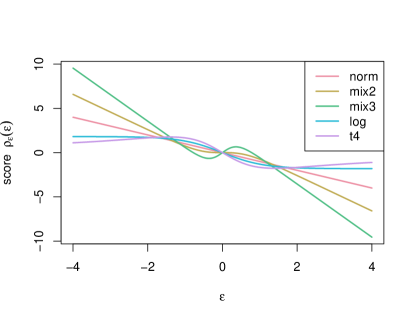
Figure 1: Score functions for the choices of distribution for $\varepsilon_{P}$ in our numerical experiments. All these distributions have mean zero and variance one. The pink line corresponds to a standard Gaussian (13), the gold and greed lines to Gaussian mixtures (14) and (15), the blue line to the logistic distribution (16), and the purple line to the Student’s $t$ distribution with 4 degrees of freedom (17).

5.1.2 401k dataset

To examine misspecification of the location–scale model for $(X,Z)$, we import the 401k data set from the DoubleML R package [Bach et al., 2021]. We take $X$ to be the income feature, and $Z$ to be age, education, family size, marriage, two-earner household, defined benefit pension, individual retirement account, home ownership, and 401k availability, giving $p=10$. We make use of all the observations ($n=9915$), and centre and scale the predictors before generating the simulated response variables.

5.1.3 Simulated responses

For the choices of regression function $f_{P}$, first define the following sinusoidal and sigmoidal families of functions:

$$f_{\text{sino}}(u;a) =\exp(-u^{2}/2)\sin(au);$$

$$f_{\text{sigm}}(u;s) =(1+\exp(-su))^{-1};$$

for $u\in\mathbb{R}$, $a,s>0$. We use the following choices for $f_{P}:\mathbb{R}\times\mathcal{Z}\to\mathbb{R}$, giving partially linear, additive, and interaction settings:

$$f_{\text{plm}}(x,z) =x+f_{\text{sigm}}(z_{2};s=1)+f_{\text{sino}}(z_{2};a=1);$$ (18)

$$f_{\text{add}}(x,z) =f_{\text{sigm}}(x;s=1)+f_{\text{sino}}(x;a=1)+f_{\text{sino}}(z_{2};a=3);$$ (19)

$$f_{\text{int}}(x,z) =f_{\text{sigm}}(x;s=3)+f_{\text{sino}}(x;a=3)+f_{\text{sino}}(z_{2};a=3)+x\times z_{2}.$$ (20)

5.2 Results

We examine the coverage of the confidence intervals for each of the 5 methods in each of the 18 settings described. Figures 2, 3, and 4 show nominal 95% confidence intervals from each of 1000 repeated experiments. We find that our method achieves at least 87% coverage in each of the 18 settings trialed and in most settings coverage is close to the desired 95%. Moreover, the estimator appears to be unbiased in most cases, with those confidence intervals not covering the parameter being equally likely to fall above or below the true parameter. In additional results which we do not include here, we find that our multivariate score estimation procedure reduces the bias as compared to the high-dimensional basis approach, and our resmoothing reduces the variance compared to numerical differencing. Taken together, our proposed estimator performs well in all settings considered.

The numerical difference and quadratic basis approach also performs reasonably well: it typically has a slightly lower variance than the resmoothing and spline-based approach, as evidenced by the slightly shorter median confidence interval widths in the additive and partially linear model examples. However, this comes at the expense of introducing noticeable bias in most settings. Indeed, the bulk of the confidence intervals failing to cover the true parameter often lie on one side of it. The confidence intervals also tend to undercover, in the worst case achieving a coverage of 78%. In some of the settings where the error distribution has heavier tails, a proportion of the confidence intervals produced are very wide (extending far beyond the margins of the plot).

As one would expect, the doubly-robust partially linear regression does very well when the partially linear model is correctly specified (18) — achieving full coverage with narrow confidence intervals — but risks completely losing coverage when the response is non-linear in $X$. Interestingly, the quadratic basis approach of Rothenhäusler and Yu [2020] displayed a similar tendency. As expected, the ordinary least squares approach did not achieve close to the specified coverage in any setting.

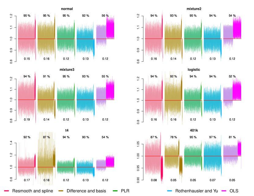
Figure 2: Estimated confidence intervals from the partially linear model experiment (18). The subplots correspond to different settings for predictor $(X,Z)$ generation. The different colours refer to the different methods. The red horizontal lines correspond to the population level target parameter. The percentages above each subplot refer to the achieved coverage (specified level 95%), and the decimals below give the median confidence interval width. In the bottom left subplot — setting (17) — some of the confidence intervals for the numerical difference and basis score approach extend significantly beyond the plotting limits.

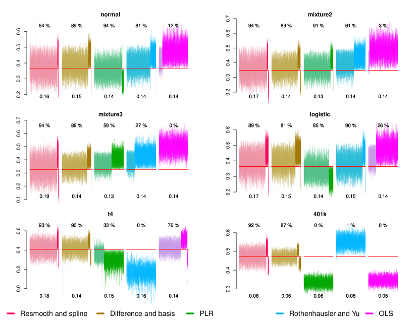
Figure 3: Estimated confidence intervals from the additive model experiment (19). The subplots correspond to different settings for predictor $(X,Z)$ generation. The different colours refer to the different methods. The red horizontal lines correspond to the population level target parameter. The percentages above each subplot refer to the achieved coverage (specified level 95%), and the decimals below give the median confidence interval width.

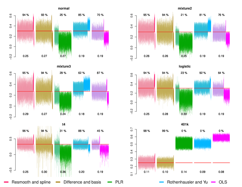
Figure 4: Estimated confidence intervals from the interaction model experiment (20). The subplots correspond to different settings for predictor $(X,Z)$ generation. The different colours refer to the different methods. The red horizontal lines correspond to the population level target parameter. The percentages above each subplot refer to the achieved coverage (specified level 95%), and the decimals below give the median confidence interval width. In the bottom left subplot — setting (17) — some of the confidence intervals for the numerical difference and basis score approach extend significantly beyond the plotting limits.

6 Discussion

The average partial effect is of interest in nonparametric regression settings, giving a single parameter summary of the effect of a predictor. In this work we have suggested a framework to enable the use of arbitrary machine learning regression procedures when doing inference on average partial effects. We propose kernel resmoothing of a first-stage machine learning method to yield a new, differentiable regression estimate. Theorem 3 demonstrates the attractive properties of this approach for a range of kernel bandwidths. We further advocate location–scale modelling for multivariate (conditional) score estimation, which we prove reduces this challenging problem to the better studied, univariate case (Theorems 5, 6, and 7). Our proofs rely on a novel result of independent interest: that Lipschitz score functions yield sub-Gaussian random variables (Theorem 4).

Appendix A Proofs in Section 2

A.1 Proof of Proposition 1

Proof.

Fix some $(x_{-j},z)\in\mathbb{R}^{d-1}\times\mathcal{Z}$ where $z$ has positive marginal density. By the product rule,

$$\nabla_{j}\big{(}g(x,z)p_{P}(x\mid z)\big{)} =\nabla_{j}g(x,z)p_{P}(x\mid z)+g(x,z)\nabla_{j}p_{P}(x\mid z)$$

$$=\nabla_{j}g(x,z)p_{P}(x\mid z)+\rho_{P,j}(x,z)g(x,z)p_{P}(x\mid z).$$

Therefore writing

$$q_{a,b}(x,z):=\{\nabla_{j}g(x,z)p_{P}(x\mid z)+\rho_{P,j}(x,z)g(x,z)p_{P}(x\mid z)\}\mathbbm{1}_{[a,b]}(x_{j}),$$

for any $-\infty<a<b<\infty$ we have

$$\int_{-\infty}^{\infty}q_{a,b}(x,z)\;dx_{j}=\int_{a}^{b}\nabla_{j}\big{(}g(x,z)p_{P}(x\mid z)\big{)}\;dx_{j}=g(b,x_{-j},z)p_{P}(b,x_{-j}\mid z)-g(a,x_{-j},z)p_{P}(a,x_{-j}\mid z).$$

Note that

$$q_{a,b}(x,z)\leq|\nabla_{j}g(x,z)p_{P}(x\mid z)+\rho_{P,j}(x,z)g(x,z)p_{P}(x\mid z)|$$

and

$$\int_{-\infty}^{\infty}|\nabla_{j}g(x,z)p_{P}(x\mid z)+\rho_{P,j}(x,z)g(x,z)p_{P}(x\mid z)|\;dx_{j}<\infty,$$

the final inequality coming from Fubini’s theorem and condition (1). Let sequences $(a_{n})$ and $(b_{n})$ be as in the statement of the theorem. By dominated convergence theorem

$$\int_{-\infty}^{\infty}\{\nabla_{j}g(x,z)p_{P}(x\mid z)+\rho_{P,j}(x,z)g(x,z)p_{P}(x\mid z)\}\;dx_{j}=\lim_{n\to\infty}\int_{-\infty}^{\infty}q_{a_{n},b_{n}}(x,z)\;dx_{j}=0.$$

As this hold for every $(x_{-j},z)$ for which $z$ has positive marginal density, integrating over $x_{-j}$ and then taking a further expectation over $Z$ proves the claim. ∎

A.2 Proof of Theorem 2

Proof.

In an abuse of notation, we refer to the quantities

$$A_{f}^{(n,k)}:=\mathbb{E}_{P}\big{[}\{f_{P}(X,Z)-\hat{f}^{(n,1)}(X,Z)\}^{2}\;\big{|}\;D^{(n,1)}\big{]},$$

for each fold $k=1,\ldots,K$. Each $A_{f}^{(n,k)}$ satisfies the same probabilistic assumptions as $A_{f}^{(n)}=A_{f}^{(n,1)}$ due to the equal partitioning and i.i.d. data. Likewise we define $A_{\rho}^{(n,k)},E_{f}^{(n,k)},E_{\rho}^{(n,k)}$.

To show the first conclusion we first highlight the term which converges to a standard normal distribution, and then deal with the remainder. Note that the lower bound on the minimum eigenvalue of $\Sigma_{P}$ corresponds to an upper bound on the maximal eigenvalue of $(\Sigma_{P})^{-1/2}$. Denote the random noise in $Y$ as

$$\xi_{P} =Y-f_{P}(X,Z);$$

$$\xi_{P,i} =y_{i}-f_{P}(x_{i},z_{i}),$$

so that $\mathbb{E}_{P}(\xi_{P}\mid X,Z)=0$.

With these preliminaries, we have

$$\sqrt{n}(\Sigma_{P})^{-1/2}\Big{(}\hat{\theta}^{(n)}-\theta_{P}\Big{)}=\frac{1}{\sqrt{n}}\sum_{i=1}^{n}(\Sigma_{P})^{-1/2}\psi_{P}(y_{i},x_{i},z_{i})+(\Sigma_{P})^{-1/2}\sum_{k=1}^{K}R_{P}^{(n,k)},$$

where the uniform central limit theorem (Lemma 8) applies to the first term and

$$R_{P}^{(n,k)}:=\frac{1}{\sqrt{n}}\sum_{i\in I^{(n,k)}}\nabla\hat{f}^{(n,k)}(x_{i},z_{i})-\hat{\rho}^{(n,k)}(x_{i},z_{i})\{y_{i}-\hat{f}^{(n,k)}(x_{i},z_{i})\}-\nabla f_{P}(x_{i},z_{i})+\rho_{P}(x_{i},z_{i})\xi_{P,i}.$$

Note that, conditionally on $D^{(n,k)}$, each summand of $R_{P}^{(n,k)}$ is i.i.d. To show that $R_{P}^{(n,k)}=o_{\mathcal{P}}(1)$, we fix some element $j\in\{1,\ldots,d\}$ and decompose

$$R_{P,j}^{(n,k)}=a^{(n,k)}-b_{f}^{(n,k)}+b_{\rho}^{(n,k)},$$ (21)

where

$$a^{(n,k)} :=\frac{1}{\sqrt{n}}\sum_{i\in I^{(n,k)}}\{\rho_{P,j}(x_{i},z_{i})-\hat{\rho}_{j}^{(n,k)}(x_{i},z_{i})\}\{f_{P}(x_{i},z_{i})-\hat{f}^{(n,k)}(x_{i},z_{i})\};$$

$$b_{f}^{(n,k)} :=\frac{1}{\sqrt{n}}\sum_{i\in I^{(n,k)}}[\nabla_{j}f_{P}(x_{i},z_{i})-\nabla_{j}\hat{f}^{(n,k)}(x_{i},z_{i})+\rho_{P,j}(x_{i},z_{i})\{f_{P}(x_{i},z_{i})-\hat{f}^{(n,k)}(x_{i},z_{i})\}];$$

$$b_{\rho}^{(n,k)} :=\frac{1}{\sqrt{n}}\sum_{i\in I^{(n,k)}}\{\rho_{P,j}(x_{i},z_{i})-\hat{\rho}_{j}^{(n,k)}(x_{i},z_{i})\}\xi_{P,i}.$$

We now show that each term is $o_{\mathcal{P}}(1)$, so Lemma 10 yields the first conclusion.

By the Cauchy–Schwarz inequality, we have

$$\mathbb{E}_{P}[|a^{(n,k)}|\mid D^{(n,k)}] \leq\sqrt{n}\mathbb{E}_{P}[|\rho_{P,j}(X,Z)-\hat{\rho}_{j}^{(n,k)}(X,Z)||f_{P}(X,Z)-\hat{f}^{(n,k)}(X,Z)|\mid D^{(n,k)}]$$

$$\leq\sqrt{nA_{f}^{(n,k)}A_{\rho}^{(n,k)}}=o_{\mathcal{P}}(1),$$

so $a^{(n,k)}$ is $o_{\mathcal{P}}(1)$ by Lemma 11. Note that each summand of $b^{(n,k)}_{\rho}$ is mean-zero conditionally on $X$ and $Z$. This means that

$$\mathbb{E}_{P}[(b^{(n,k)}_{\rho})^{2}\mid D^{(n,k)}] =\mathbb{E}_{P}[\{\rho_{P,j}(X,Z)-\hat{\rho}^{(n,k)}_{j}(X,Z)\}^{2}\mathbb{E}_{P}(\xi_{P}^{2}\mid X,Z)\mid D^{(n,k)}]$$

$$\leq E_{\rho}^{(n,k)}=o_{\mathcal{P}}(1).$$

Again using Lemma 11 we have that $b^{(n,k)}_{\rho}=o_{\mathcal{P}}(1)$.

We now apply a similar argument to $b^{(n,k)}_{f}$, using Proposition 1 to show that each summand is mean zero. Given $\epsilon>0$, noting that both $A_{f}^{(n,k)}$ and $E_{f}^{(n,k)}$ are $O_{\mathcal{P}}(1)$, we have there exists $M$ and $N\in\mathbb{N}$ such that for sequences of $D^{(n,k)}$-measurable events $\Omega_{P,n}$ with $\mathbb{P}_{P}(\Omega_{P,n})\geq 1-\epsilon$, for all $n\geq N$,

$$\mathbb{E}_{P}\Big{[}\big{|}f_{P}(X,Z)-\hat{f}^{(n,k)}(X,Z)\big{|}\;\Big{|}\;D^{(n,k)}\Big{]}\mathbbm{1}_{\Omega_{P,n}} <M;$$ (22)

$$\mathbb{E}_{P}\Big{[}\big{|}\nabla_{j}f_{P}(X,Z)-\nabla_{j}\hat{f}^{(n,k)}(X,Z)+\rho_{P,j}\big{\{}f_{P}(X,Z)-\hat{f}^{(n,k)}(X,Z)\big{\}}\big{|}\;\Big{|}\;D^{(n,k)}\Big{]}\mathbbm{1}_{\Omega_{P,n}} <M.$$ (23)

Now fixing $z,x_{-j}$ (where $x_{-j}\in\mathbb{R}^{d-1}$), we have that the function

$$\Big{(}f_{P}\big{(}(\cdot,x_{-j}),z\big{)}-\hat{f}^{(n,k)}\big{(}(\cdot,x_{-j}),z\big{)}\Big{)}p\big{(}(\;\cdot\;,x{{}_{-}j})\;\big{|}\;z\big{)}$$

is continuous, where we understand $(u,x_{-j})=(x_{1},\ldots,x_{j-1},u,x_{j+1},\ldots,x_{d})$ for $u\in\mathbb{R}$. We may therefore apply Lemma 21 to both

$$t \mapsto\Big{(}f_{P}\big{(}(t,x_{-j}),z\big{)}-\hat{f}^{(n,k)}\big{(}(t,x_{-j}),z\big{)}\Big{)}p\big{(}(t,x_{-j})\;\big{|}\;z\big{)}$$

$$t \mapsto\Big{(}f_{P}\big{(}(-t,x_{-j}),z\big{)}-\hat{f}^{(n,k)}\big{(}(-t,x_{-j}),z\big{)}\Big{)}p\big{(}(-t,x_{-j})\;\big{|}\;z\big{)}.$$

This, in combination with (22) implies that on $\Omega_{P,n}$ and for each $n\geq N$, there exist $D^{(n,k)}$-measurable sequences $a_{P,m}\to-\infty$, $b_{P,m}\to\infty$ such that

$$\lim_{m\to\infty}\bigg{\{}\Big{(}f_{P}\big{(}(b_{P,m},x_{-j}),z\big{)}-\hat{f}^{(n,k)}\big{(}(b_{P,m},x_{-j}),z\big{)}\Big{)}p\big{(}(b_{P,m},x_{-j})\;\big{|}\;z\big{)}\phantom{\bigg{\}}}$$

$$-\big{(}f_{P}\big{(}(a_{P,m},x_{-j}),z\big{)}-\hat{f}^{(n,k)}\big{(}(a_{P,m},x_{-j}),z\big{)}\Big{)}p\big{(}(a_{P,m},x_{-j})\;\big{|}\;z\big{)}\bigg{\}} =0.$$ (24)

Equations (23 and 24) verify that we may apply Proposition 1 conditionally on $D^{(n,k)}$. Therefore, for all $n$ sufficiently large,

$$\mathbb{E}_{P}\Big{[}\nabla_{j}f_{P}(X,Z)-\nabla_{j}\hat{f}^{(n,k)}(X,Z)+\rho_{P,j}\big{\{}f_{P}(X,Z)-\hat{f}^{(n,k)}(X,Z)\big{\}}\;\Big{|}\;D^{(n,k)}\Big{]}\mathbbm{1}_{\Omega_{P,n}}\ =0$$

and hence

$$\mathbb{E}_{P}[(b^{(n,k)}_{f})^{2}\mid D^{(n,k)}]\mathbbm{1}_{\Omega_{P,n}}$$

$$=\; \mathbb{E}_{P}([\nabla_{j}f_{P}(X,Z)-\nabla_{j}\hat{f}^{(n,k)}(X,Z)+\rho_{P,j}(X,Z)\{f_{P}(X,Z)-\hat{f}^{(n,k)}(X,Z)\}]^{2}\mid D^{(n,k)})\mathbbm{1}_{\Omega_{P,n}}$$

$$\leq\; E_{f}^{(n,k)}.$$

Now

$$\mathbb{P}_{P}(b^{(n,k)}_{f}>\epsilon)\leq\mathbb{P}_{P}(b^{(n,k)}_{f}\mathbbm{1}_{\Omega_{P,n}}>\epsilon)+\mathbb{P}_{P}(\Omega_{P,n}^{c})\leq\mathbb{P}_{P}(b^{(n,k)}_{f}\mathbbm{1}_{\Omega_{P,n}}>\epsilon)+\epsilon.$$

Lemma 11 shows that the first term above converges to $0$, uniformly in $P$, and so $b_{f}^{(n,k)}$ is $o_{\mathcal{P}}(1)$.

Turning now to the second conclusion, we aim to show that $\hat{\Sigma}^{(n)}-\Sigma_{P}=o_{\mathcal{P}}(1)$. We introduce notation for the following random functions:

$$\hat{\psi}^{(n,k)}(y,x,z):=\nabla\hat{f}^{(n,k)}(x,z)-\hat{\rho}^{(n,k)}(x,z)\{y-\hat{f}^{(n,k)}(x,z)\}-\hat{\theta}^{(n)}.$$

We will focus on an individual element $(\hat{\Sigma}^{(n)}-\Sigma_{P})_{l,m}$, $1\leq l,m\leq d$, and make use of Lemma 9. We first check that

$$\sup_{P\in\mathcal{P}}\mathbb{E}_{P}\Big{[}\big{|}\psi_{P,l}(Y,X,Z)\psi_{P,m}(Y,X,Z)-\mathbb{E}_{P}[\psi_{P,l}(Y,X,Z)\psi_{P,m}(Y,X,Z)]\big{|}^{1+\tilde{\eta}}\Big{]}\leq\tilde{c},$$

for some $\tilde{\eta},\tilde{c}>0$. Indeed, due to the convexity of $x\mapsto|x|^{1+\tilde{\eta}}$,

$$\mathbb{E}_{P}\Big{[}\big{|}\psi_{P,l}(Y,X,Z)\psi_{P,m}(Y,X,Z) -\mathbb{E}_{P}[\psi_{P,l}(Y,X,Z)\psi_{P,m}(Y,X,Z)]\big{|}^{1+\tilde{\eta}}\Big{]}$$

$$\leq 2^{\tilde{\eta}}\Big{\{}\mathbb{E}_{P}\Big{[}\big{|}\psi_{P,l}(Y,X,Z)\psi_{P,m}(Y,X,Z)\big{|}^{1+\tilde{\eta}}\Big{]}$$

$$\phantom{\leq}+\Big{|}\mathbb{E}_{P}[\psi_{P,l}(Y,X,Z)\psi_{P,m}(Y,X,Z)]\Big{|}^{1+\tilde{\eta}}\Big{\}}$$

$$\leq 2^{1+\tilde{\eta}}\mathbb{E}_{P}\Big{[}\big{|}\psi_{P,l}(Y,X,Z)\psi_{P,m}(Y,X,Z)\big{|}^{1+\tilde{\eta}}\Big{]}$$

$$\leq 2^{1+\tilde{\eta}}\mathbb{E}_{P}\Big{[}\|\psi_{P}(Y,X,Z)\|_{2}^{2+2\tilde{\eta}}\Big{]}.$$

The first inequality is $|(a+b)/2|^{1+\tilde{\eta}}\leq(|a|^{1+\tilde{\eta}}+|b|^{1+\tilde{\eta}})/2$, the second is Jensen’s inequality, and the final inequality is $|ab|\leq(a^{2}+b^{2})/2$. Therefore the condition is satisfied for $\tilde{\eta}=\eta/2$, $\tilde{c}=2^{1+\eta/2}c_{2}$.

We are now ready to decompose the covariance estimation error.

$$(\hat{\Sigma}^{(n)}-\Sigma_{P})_{l,m} =\frac{1}{n}\sum_{k=1}^{K}\sum_{i\in I^{(n,k)}}\hat{\psi}_{l}^{(n,k)}(y_{i},x_{i},z_{i})\hat{\psi}_{m}^{(n,k)}(y_{i},x_{i},z_{i})-\mathbb{E}_{P}[\psi_{P,l}(Y,X,Z)\psi_{P,m}(Y,X,Z)]$$

$$=\frac{1}{n}\sum_{i=1}^{n}\Big{[}\psi_{P,l}(y_{i},x_{i},z_{i})\psi_{P,m}(y_{i},x_{i},z_{i})-\mathbb{E}_{P}[\psi_{P,l}(Y,X,Z)\psi_{P,m}(Y,X,Z)]\Big{]}+\frac{1}{K}\sum_{k=1}^{K}S_{P}^{(n,k)},$$

where the first term is $o_{\mathcal{P}}(1)$ by Lemma 9 and

$$S_{P}^{(n,k)}:=\frac{K}{n}\sum_{i\in I^{(n,k)}}\Big{[}\hat{\psi}_{l}^{(n,k)}(y_{i},x_{i},z_{i})\hat{\psi}_{m}^{(n,k)}(y_{i},x_{i},z_{i})-\psi_{P,l}(y_{i},x_{i},z_{i})\psi_{P,m}(y_{i},x_{i},z_{i})\Big{]}.$$

We show that $S_{P}^{(n,k)}=o_{\mathcal{P}}(1)$ using the following identity for $a_{1},a_{2},b_{1},b_{2}\in\mathbb{R}$,

$$a_{1}b_{1}-a_{2}b_{2}=(a_{1}-a_{2})(b_{1}-b_{2})+a_{2}(b_{1}-b_{2})+b_{2}(a_{1}-a_{2}),$$

and then applying the Cauchy–Schwarz inequality to each term.

$$\big{|}S_{P}^{(n,k)}\big{|} =\bigg{|}\frac{K}{n}\sum_{i\in I^{(n,k)}}\hat{\psi}_{l}^{(n,k)}(y_{i},x_{i},z_{i})\hat{\psi}_{m}^{(n,k)}(y_{i},x_{i},z_{i})-\psi_{P,l}(y_{i},x_{i},z_{i})\psi_{P,m}(y_{i},x_{i},z_{i})\bigg{|}$$

$$\leq\bigg{|}\frac{K}{n}\sum_{i\in I^{(n,k)}}\Big{\{}\hat{\psi}_{l}^{(n,k)}(y_{i},x_{i},z_{i})-\psi_{P,l}(y_{i},x_{i},z_{i})\Big{\}}\Big{\{}\hat{\psi}_{m}^{(n,k)}(y_{i},x_{i},z_{i})-\psi_{P,m}(y_{i},x_{i},z_{i})\Big{\}}\bigg{|}$$

$$\phantom{=}+\bigg{|}\frac{K}{n}\sum_{i\in I^{(n,k)}}\Big{\{}\hat{\psi}_{l}^{(n,k)}(y_{i},x_{i},z_{i})-\psi_{P,l}(y_{i},x_{i},z_{i})\Big{\}}\psi_{P,m}(y_{i},x_{i},z_{i})\bigg{|}$$

$$\phantom{=}+\bigg{|}\frac{K}{n}\sum_{i\in I^{(n,k)}}\Big{\{}\hat{\psi}_{m}^{(n,k)}(y_{i},x_{i},z_{i})-\psi_{P,m}(y_{i},x_{i},z_{i})\Big{\}}\psi_{P,l}(y_{i},x_{i},z_{i})\bigg{|}$$

$$\leq\bigg{[}\frac{K}{n}\sum_{i\in I^{(n,k)}}\Big{\{}\hat{\psi}_{l}^{(n,k)}(y_{i},x_{i},z_{i})-\psi_{P,l}(y_{i},x_{i},z_{i})\Big{\}}^{2}\bigg{]}^{1/2}$$

$$\phantom{=}\cdot\bigg{[}\frac{K}{n}\sum_{i\in I^{(n,k)}}\Big{\{}\hat{\psi}_{m}^{(n,k)}(y_{i},x_{i},z_{i})-\psi_{P,m}(y_{i},x_{i},z_{i})\Big{\}}^{2}\bigg{]}^{1/2}$$

$$\phantom{=}+\bigg{[}\frac{K}{n}\sum_{i\in I^{(n,k)}}\Big{\{}\hat{\psi}_{l}^{(n,k)}(y_{i},x_{i},z_{i})-\psi_{P,l}(y_{i},x_{i},z_{i})\Big{\}}^{2}\bigg{]}^{1/2}\bigg{[}\frac{K}{n}\sum_{i\in I^{(n,k)}}\psi_{P,m}(y_{i},x_{i},z_{i})^{2}\Bigg{]}^{1/2}$$

$$\phantom{=}+\bigg{[}\frac{K}{n}\sum_{i\in I^{(n,k)}}\Big{\{}\hat{\psi}_{m}^{(n,k)}(y_{i},x_{i},z_{i})-\psi_{P,m}(y_{i},x_{i},z_{i})\Big{\}}^{2}\bigg{]}^{1/2}\bigg{[}\frac{K}{n}\sum_{i\in I^{(n,k)}}\psi_{P,l}(y_{i},x_{i},z_{i})^{2}\bigg{]}^{1/2}.$$

Therefore it suffices to show that, for each $l=1,\ldots,d$,

$$T_{P,1}^{(n,k)} :=\frac{K}{n}\sum_{i\in I^{(n,k)}}\psi_{P,l}(y_{i},x_{i},z_{i})^{2}=O_{\mathcal{P}}(1);$$

$$T_{P,2}^{(n,k)} :=\frac{K}{n}\sum_{i\in I^{(n,k)}}\Big{\{}\hat{\psi}_{l}^{(n,k)}(y_{i},x_{i},z_{i})-\psi_{P,l}(y_{i},x_{i},z_{i})\Big{\}}^{2}=o_{\mathcal{P}}(1).$$

To this end, Lemma 9 gives $T_{P,1}^{(n,k)}=(\Sigma_{P})_{(l,l)}+o_{\mathcal{P}}(1)$. Moreover, similarly to equation (21) and using the inequality $(a+b+c+d)^{2}\leq 4(a^{2}+b^{2}+c^{2}+d^{2})$,

$$T_{P,2}^{(n,k)} =\frac{K}{n}\sum_{i\in I^{(n,k)}}\Big{\{}\hat{\psi}_{l}^{(n,k)}(y_{i},x_{i},z_{i})-\psi_{P,l}(y_{i},x_{i},z_{i})\Big{\}}^{2}$$

$$=\frac{K}{n}\sum_{i\in I^{(n,k)}}\Big{[}\Big{\{}\rho_{P,l}(x_{i},z_{i})-\hat{\rho}_{l}^{(n,k)}(x_{i},z_{i})\Big{\}}\Big{\{}f_{P}(x_{i},z_{i})-\hat{f}^{(n,k)}(x_{i},z_{i})\Big{\}}$$

$$\phantom{=}-\nabla_{l}f_{P}(x_{i},z_{i})+\nabla_{l}\hat{f}^{(n,k)}(x_{i},z_{i})-\rho_{P,l}(x_{i},z_{i})\Big{\{}f_{P}(x_{i},z_{i})-\hat{f}^{(n,k)}(x_{i},z_{i})\Big{\}}$$

$$\phantom{=}+\Big{\{}\rho_{P,l}(x_{i},z_{i})-\hat{\rho}_{l}^{(n,k)}(x_{i},z_{i})\Big{\}}\xi_{P,i}-\hat{\theta}_{l}^{(n)}+\theta_{P,l}\Big{]}^{2}$$

$$\leq 4\{\tilde{a}^{(n,k)}+\tilde{b}_{f}^{(n,k)}+\tilde{b}_{\rho}^{(n,k)}+(\hat{\theta}_{l}^{(n)}-\theta_{P,l})^{2}\},$$

where

$$\tilde{a}^{(n,k)} :=\frac{K}{n}\sum_{i\in I^{(n,k)}}\Big{\{}\rho_{P,l}(x_{i},z_{i})-\hat{\rho}_{l}^{(n,k)}(x_{i},z_{i})\Big{\}}^{2}\Big{\{}f_{P}(x_{i},z_{i})-\hat{f}^{(n,k)}(x_{i},z_{i})\Big{\}}^{2};$$

$$\tilde{b}_{f}^{(n,k)} :=\frac{K}{n}\sum_{i\in I^{(n,k)}}\left[\nabla_{l}f_{P}(x_{i},z_{i})-\nabla_{l}\hat{f}^{(n,k)}(x_{i},z_{i})+\rho_{P,l}(x_{i},z_{i})\left\{f_{P}(x_{i},z_{i})-\hat{f}^{(n,k)}(x_{i},z_{i})\right\}\right]^{2};$$

$$\tilde{b}_{\rho}^{(n,k)} :=\frac{K}{n}\sum_{i\in I^{(n,k)}}\Big{\{}\rho_{P,l}(x_{i},z_{i})-\hat{\rho}_{l}^{(n,k)}(x_{i},z_{i})\Big{\}}^{2}\xi_{P,i}^{2}.$$

Since $n^{-1/2}(\hat{\theta}^{(n)}-\theta_{P})$ is uniformly asympotically Gaussian, we have that $(\hat{\theta}_{l}^{(n)}-\theta_{P,l})^{2}=O_{\mathcal{P}}(n^{-1})$. For $\tilde{a}^{(n,k)}$, $\tilde{b}_{f}^{(n,k)}$ and $\tilde{b}_{\rho}^{(n,k)}$ we use Lemma 11, noting that conditionally on $D^{(n,k)}$ each summand is i.i.d.

Using the identity $\sum_{i}a_{i}b_{i}\leq(\sum_{i}a_{i})(\sum_{i}b_{i})$ for positive sequences $(a_{i})$ and $(b_{i})$, we have

$$\big{|}\tilde{a}^{(n,k)}\big{|}\leq\frac{n}{K}\tilde{a}_{\rho}^{(n,k)}\tilde{a}_{f}^{(n,k)},$$

for

$$\tilde{a}_{\rho}^{(n,k)} :=\frac{K}{n}\sum_{i\in I^{(n,k)}}\Big{\{}\rho_{P,l}(x_{i},z_{i})-\hat{\rho}_{l}^{(n,k)}(x_{i},z_{i})\Big{\}}^{2};$$

$$\tilde{a}_{f}^{(n,k)} :=\frac{K}{n}\sum_{i\in I^{(n,k)}}\Big{\{}f_{P}(x_{i},z_{i})-\hat{f}^{(n,k)}(x_{i},z_{i})\Big{\}}^{2}.$$

Finally,

$$\mathbb{E}_{P}\Big{(}\big{|}\tilde{a}_{f}^{(n,k)}\big{|}\;\Big{|}\;D^{(n,k)}\Big{)} =\mathbb{E}_{P}\Big{[}\big{\{}f_{P}(X,Z)-\hat{f}^{(n,k)}(X,Z)\big{\}}^{2}\;\Big{|}\;D^{(n,k)}\Big{]}$$

$$\leq A_{f}^{(n,k)};$$

$$\mathbb{E}_{P}\Big{(}\big{|}\tilde{a}_{\rho}^{(n,k)}\big{|}\;\Big{|}\;D^{(n,k)}\Big{)} =\mathbb{E}_{P}\Big{[}\big{\{}\rho_{P,l}(X,Z)-\hat{\rho}_{l}^{(n,k)}(X,Z)\big{\}}^{2}\;\Big{|}\;D^{(n,k)}\Big{]}$$

$$\leq A_{\rho}^{(n,k)};$$

$$\mathbb{E}_{P}\Big{(}\big{|}\tilde{b}_{f}^{(n,k)}\big{|}\;\Big{|}\;D^{(n,k)}\Big{)} =\mathbb{E}_{P}\Big{(}\big{[}\nabla_{l}f_{P}(X,Z)-\nabla_{l}\hat{f}^{(n,k)}(X,Z)+\rho_{P,l}(X,Z)\big{\{}f_{P}(X,Z)-\hat{f}^{(n,k)}(X,Z)\big{\}}\big{]}^{2}\;\Big{|}\;D^{(n,k)}\Big{)}$$

$$\leq E_{f}^{(n,k)};$$

$$\mathbb{E}_{P}\Big{(}\big{|}\tilde{b}_{\rho}^{(n,k)}\big{|}\;\Big{|}\;D^{(n,k)}\Big{)} =\mathbb{E}_{P}\Big{[}\big{\{}\rho_{P,l}(X,Z)-\hat{\rho}_{l}^{(n,k)}(X,Z)\big{\}}^{2}\xi_{P}^{2}\;\Big{|}\;D^{(n,k)}\Big{]}$$

$$\leq E_{\rho}^{(n,k)}.$$

This suffices to show that $T^{(n,k)}_{P,2}=o_{\mathcal{P}}(1)$, so $\hat{\Sigma}^{(n)}-\Sigma_{P}=o_{\mathcal{P}}(1)$.

It remains to show the final conclusion. By Lemma 10, it is enough to show that

$$(\Sigma_{P})^{-1/2}(\hat{\Sigma}^{(n)})^{1/2}=I+o_{\mathcal{P}}(1).$$

We have that the maximal eigenvalue of $(\Sigma_{P})^{-1/2}$ is uniformly bounded above, and further that

$$(\Sigma_{P})^{-1/2}(\hat{\Sigma}^{(n)})^{1/2} =(\Sigma_{P})^{-1/2}\big{\{}(\hat{\Sigma}^{(n)})^{1/2}-(\Sigma_{P})^{1/2}+(\Sigma_{P})^{1/2}\big{\}}$$

$$=I+(\Sigma_{P})^{-1/2}\big{\{}(\hat{\Sigma}^{(n)})^{1/2}-(\Sigma_{P})^{1/2}\big{\}}.$$

Therefore it remains to check that

$$(\hat{\Sigma}^{(n)})^{1/2}=(\Sigma_{P})^{1/2}+o_{\mathcal{P}}(1).$$

By Horn and Johnson [1985, Eqn. (7.2.13)],

$$\big{\|}(\hat{\Sigma}^{(n)})^{1/2}-(\Sigma_{P})^{1/2}\big{\|}_{2} \leq\big{\|}(\Sigma_{P})^{-1/2}\big{\|}_{2}\|\hat{\Sigma}^{(n)}-\Sigma_{P}\|_{2}$$

$$\leq c_{1}^{-1/2}\|\hat{\Sigma}^{(n)}-\Sigma_{P}\|_{2}.$$

Hence $(\hat{\Sigma}^{(n)})^{1/2}-(\Sigma_{P})^{1/2}=o_{\mathcal{P}}(1)$. This completes the proof. ∎

A.3 Auxiliary lemmas

Lemma 8 (Shah and Peters [2020, Supp. Lem. 18], vectorised).

Let $\mathcal{P}$ be a family of distributions for $\zeta\in\mathbb{R}^{d}$ and suppose $\zeta_{1},\zeta_{2},\dots$ are i.i.d. copies. For each $n\in\mathbb{N}$, let $S_{n}=n^{-1/2}\sum_{i=1}^{n}\zeta_{i}$. Suppose that for all $P\in\mathcal{P}$, we have $E_{P}(\zeta)=0$, $\mathrm{Var}_{P}(\zeta)=I$, and $\mathbb{E}_{P}(\|\zeta\|_{2}^{2+\eta})\leq c$ for some $c,\eta>0$. Then we have that

$$\lim_{n\to\infty}\sup_{P\in\mathcal{P}}\sup_{t\in\mathbb{R}^{d}}|\mathbb{P}_{P}(S_{n}\leq t)-\Phi(t)|=0.$$

Proof.

For each $n$, let $P_{n}\in\mathcal{P}$ satisfy

$$\sup_{P\in\mathcal{P}}\sup_{t\in\mathbb{R}^{d}}|\mathbb{P}_{P}(S_{n}\leq t)-\Phi(t)|\leq\sup_{t\in\mathbb{R}^{d}}|\mathbb{P}_{P_{n}}(S_{n}\leq t)-\Phi(t)|+n^{-1}.$$

Let $Y_{n,i}$ be equal in distribution to $n^{-1/2}\zeta_{i}$ under $P_{n}$. We check the conditions to apply van der Vaart [1998, Prop. 2.27]. Indeed, $Y_{n,1},\dots,Y_{n,n}$ are i.i.d. for each $n$, and $\sum_{i=1}^{n}\mathrm{Var}(Y_{n,i})=\sum_{i=1}^{n}n^{-1}\mathrm{Var}_{P_{n}}(\zeta)=I$. Finally, for any $\epsilon>0$ we have

$$\sum_{i=1}^{n}\mathbb{E}\big{(}\|Y_{n,1}\|_{2}^{2}\mathbbm{1}_{\{\|Y_{n,i}\|_{2}>\epsilon\}}\big{)} =\mathbb{E}_{P_{n}}\big{(}\|\zeta\|_{2}^{2}\mathbbm{1}_{\{\|\zeta\|_{2}>\sqrt{n}\epsilon\}}\big{)}$$

$$\leq\big{[}\mathbb{E}_{P_{n}}(\|\zeta\|_{2}^{2+\eta})\big{]}^{2/(2+\eta)}\big{[}\mathbb{E}_{P_{n}}\big{(}\mathbbm{1}_{\{\|\zeta\|_{2}>\sqrt{n}\epsilon\}}^{(2+\eta)/\eta}\big{)}\big{]}^{\eta/(2+\eta)}$$

$$\leq c^{2/(2+\eta)}[\mathbb{P}_{P_{n}}(\|\zeta\|_{2}>\sqrt{n}\epsilon)]^{\eta/(2+\eta)}$$

$$\leq c^{2/(2+\eta)}[\mathbb{E}_{P_{n}}(\|\zeta\|_{2})/(\sqrt{n}\epsilon)]^{\eta/(2+\eta)}$$

$$\leq c\epsilon^{-\eta/(2+\eta)}n^{-\eta/(4+2\eta)}\to 0.$$

Here the first inequality is due to Hölder, the third due to Markov and the second and fourth are applying the assumption $\mathbb{E}_{P}(\|\zeta\|_{2}^{2+\eta})\leq c$. ∎

Lemma 9 (Shah and Peters [2020, Supp. Lem. 19]).

Let $\mathcal{P}$ be a family of distributions for $\zeta\in\mathbb{R}$ and suppose $\zeta_{1},\zeta_{2},\dots$ are i.i.d. copies. For each $n\in\mathbb{N}$, let $S_{n}=n^{-1}\sum_{i=1}^{n}\zeta_{i}$. Suppose that for all $P\in\mathcal{P}$, we have $E_{P}(\zeta)=0$, and $\mathbb{E}_{P}(|\zeta|^{1+\eta})\leq c$ for some $c,\eta>0$. Then we have that for all $\epsilon>0$,

$$\lim_{n\to\infty}\sup_{P\in\mathcal{P}}\mathbb{P}_{P}(|S_{n}|>\epsilon)=0.$$

Lemma 10.

Let $\mathcal{P}$ be a family of distributions that determines the law of sequences $(V_{n})_{n\in\mathbb{N}}$ and $(W_{n})_{n\in\mathbb{N}}$ of random vectors in $\mathbb{R}^{d}$ and $(M_{n})_{n\in\mathbb{N}}$ random matrices in $\mathbb{R}^{d\times d}$. Suppose

$$\lim_{n\to\infty}\sup_{P\in\mathcal{P}}\sup_{t\in\mathbb{R}^{d}}|\mathbb{P}_{P}(V_{n}\leq t)-\Phi(t)|=0.$$

Then we have the following.

1. If $W_{n}=o_{\mathcal{P}}(1)$ we have

   $$\lim_{n\to\infty}\sup_{P\in\mathcal{P}}\sup_{t\in\mathbb{R}^{d}}|\mathbb{P}_{P}(V_{n}+W_{n}\leq t)-\Phi(t)|=0.$$

2. If $M_{n}=I+o_{\mathcal{P}}(1)$ we have

   $$\lim_{n\to\infty}\sup_{P\in\mathcal{P}}\sup_{t\in\mathbb{R}^{d}}|\mathbb{P}_{P}(M_{n}^{-1}V_{n}\leq t)-\Phi(t)|=0.$$

Proof.

We first show that for any $\delta>0$, $\sup_{t\in\mathbb{R}^{d}}|\Phi(t+\delta)-\Phi(t)|\leq d\delta$. Indeed, letting $Z\sim N(0,I)$ in $\mathbb{R}^{d}$,

$$|\Phi(t+\delta)-\Phi(t)| =\mathbb{P}(\cap_{j}\{Z_{j}\leq t_{j}+\delta\})-\mathbb{P}(\cap_{j}\{Z_{j}\leq t_{j}\})$$

$$=\mathbb{P}(\cup_{j}\{Z_{j}\in(t_{j},t_{j}+\delta]\})$$

$$\leq\sum_{j}\mathbb{P}(Z_{j}\in(t_{j},t_{j}+\delta])$$

$$\leq d\delta.$$

The final line follows because the univariate standard normal c.d.f. has Lipschitz constant $1/\sqrt{2\pi}\leavevmode\nobreak\ <\leavevmode\nobreak\ 1$.

Now consider the setup of (a). Given $\epsilon>0$ let $N$ be such that for all $n\geq N$ and for all $P\in\mathcal{P}$,

$$\sup_{t\in\mathbb{R}^{d}}|\mathbb{P}_{P}(V_{n}\leq t)-\Phi(t)|<\epsilon/3\text{\;\; and \;\;}\mathbb{P}_{P}[\|W_{n}\|_{\infty}>\epsilon/(3d)]<\epsilon/3.$$

Then

$$\mathbb{P}_{P}(V_{n}+W_{n}\leq t)-\Phi(t) =\mathbb{P}_{P}(\cap_{j}\{V_{nj}+W_{nj}\leq t_{j}\})-\Phi(t)$$

$$\leq\mathbb{P}_{P}[(\cap_{j}\{V_{nj}\leq t_{j}+\epsilon/(3d)\})\cup(\cup_{j}\{W_{nj}<-\epsilon/(3d)\})]-\Phi(t)$$

$$\leq\mathbb{P}[V_{n}\leq t+\epsilon/(3d)]+\mathbb{P}[\|W_{n}\|_{\infty}>\epsilon/(3d)]-\Phi(t)$$

$$<\epsilon/3+\Phi[t+\epsilon/(3d)]-\Phi(t)+\epsilon/3<\epsilon,$$

and

$$\mathbb{P}_{P}(V_{n}+W_{n}\leq t)-\Phi(t) =1-\Phi(t)-\mathbb{P}_{P}(\cup_{j}\{V_{nj}+W_{nj}>t_{j}\})$$

$$\geq 1-\Phi(t)-\mathbb{P}_{P}[\cup_{j}(\{V_{nj}>t_{j}-\epsilon/(3d)\}\cup\{W_{nj}>\epsilon/(3d)\})]$$

$$=1-\Phi(t)-\mathbb{P}_{P}[(\cup_{j}\{V_{nj}>t_{j}-\epsilon/(3d)\})\cup\{\|W_{n}\|_{\infty}>\epsilon/(3d)\}]$$

$$\geq 1-\Phi(t)-\mathbb{P}_{P}(\cup_{j}\{V_{nj}>t_{j}-\epsilon/(3d)\})-\mathbb{P}_{P}[\|W_{n}\|_{\infty}>\epsilon/(3d)]$$

$$>\mathbb{P}_{P}[V_{n}\leq t-\epsilon/(3d)]-\Phi(t)-\epsilon/3$$

$$>-\epsilon/3+\Phi[t-\epsilon/(3d)]-\Phi(t)-\epsilon/3>-\epsilon.$$

Thus for all $n\geq N$ and $P\in\mathcal{P}$,

$$\sup_{t\in\mathbb{R}^{d}}|\mathbb{P}_{P}(V_{n}+W_{n}\leq t)-\Phi(t)|<\epsilon.$$

To prove (b), it suffices to show that $(M_{n}^{-1}-I)V_{n}=o_{\mathcal{P}}(1)$ and then apply (a). We have that $M_{n}-I$ is $o_{\mathcal{P}}(1)$, and so the sequence

$$\|M_{n}-I\|_{\infty}:=\sup_{x:\|x\|_{\infty}=1}\|(M_{n}-I)x\|_{\infty}=o_{\mathcal{P}}(1).$$

By Golub and Van Loan [2013, Thm. 2.3.4], when $\|M_{n}-I\|_{\infty}<1$, then $M_{n}$ is nonsingular and

$$\|M_{n}^{-1}-I\|_{\infty}\leq\frac{\|M_{n}-I\|_{\infty}}{1-\|M_{n}-I\|_{\infty}}.$$

Now

$$\sup_{P\in\mathcal{P}}\mathbb{P}_{P}(\|M_{n}^{-1}-I\|_{\infty}>\epsilon) \leq\sup_{P\in\mathcal{P}}\mathbb{P}_{P}\bigg{(}\frac{\|M_{n}-I\|_{\infty}}{1-\|M_{n}-I\|_{\infty}}>\epsilon\bigg{)}$$

$$=\sup_{P\in\mathcal{P}}\mathbb{P}_{P}(\|M_{n}-I\|_{\infty}>\epsilon/(1+\epsilon))\to 0,$$

so $\|M_{n}^{-1}-I\|_{\infty}$ is also $o_{\mathcal{P}}(1)$.

Now we can show that the sequence $\|(M_{n}^{-1}-I)V_{n}\|_{\infty}$ is $o_{\mathcal{P}}(1)$. Indeed given $\epsilon>0$, let $\delta>0$ be such that $\Phi(\epsilon/\delta)>1-\epsilon/3$, and let $N$ be such that for all $n\geq N$ and for all $P\in\mathcal{P}$,

$$\sup_{t\in\mathbb{R}^{d}}|\mathbb{P}_{P}(V_{n}\leq t)-\Phi(t)|<\epsilon/3\text{\;\; and \;\;}\mathbb{P}_{P}(\|M_{n}^{-1}-I\|_{\infty}>\delta)<\epsilon/3.$$

Then

$$\mathbb{P}_{P}(\|(M_{n}^{-1}-I)V_{n}\|_{\infty}>\epsilon) \leq\mathbb{P}_{P}(\|M_{n}^{-1}-I\|_{\infty}\|V_{n}\|_{\infty}>\epsilon)$$

$$\leq\mathbb{P}_{P}(\{\|M_{n}^{-1}-I\|_{\infty}>\delta\}\cup\{\|V_{n}\|_{\infty}>\epsilon/\delta\})$$

$$\leq\mathbb{P}_{P}(\|M_{n}^{-1}-I\|_{\infty}>\delta)+1-\mathbb{P}_{P}(V_{n}\leq\epsilon/\delta)$$

$$<\epsilon/3+1-\Phi(\epsilon/\delta)+\epsilon/3<\epsilon.$$

This suffices to show that the sequence of random vectors $(M_{n}^{-1}-I)V_{n}$ is $o_{\mathcal{P}}(1)$, so we are done by (a). ∎

Lemma 11.

Let $X_{m}$ and $Y_{m}$ be sequences of random vectors governed by laws in some set $\mathcal{P}$, let $\|\cdot\|$ be any norm and $q\geq 1$.

1. If $\mathbb{E}_{P}(\|X_{m}\|^{q}\mid Y_{m})=o_{\mathcal{P}}(1)$, then $\|X_{m}\|=o_{\mathcal{P}}(1)$.

2. If $\mathbb{E}_{P}(\|X_{m}\|^{q}\mid Y_{m})=O_{\mathcal{P}}(1)$, then $\|X_{m}\|=O_{\mathcal{P}}(1)$.

Proof.

In both cases we work with a bounded version of $\|X_{m}\|$, and apply Markov’s inequality.

Let $\mathbb{E}_{P}(\|X_{m}\|^{q}\mid Y_{m})=o_{\mathcal{P}}(1)$. Given $\epsilon>0$,

$$\mathbb{P}_{P}[\|X_{m}\|>\epsilon] =\mathbb{P}_{P}[\|X_{m}\|^{q}>\epsilon^{q}]$$

$$=\mathbb{P}_{P}[(\|X_{m}\|^{q}\wedge 2\epsilon^{q})>\epsilon^{q}]$$

$$\leq\epsilon^{-q}\mathbb{E}_{P}[\|X_{m}\|^{q}\wedge 2\epsilon^{q}]$$

$$=\epsilon^{-q}\mathbb{E}_{P}[\mathbb{E}_{P}(\|X_{m}\|^{q}\mid Y_{m})\wedge 2\epsilon^{q}].$$

Writing $W_{m}=\mathbb{E}_{P}(\|X_{m}\|^{q}\mid Y_{m})\wedge 2\epsilon^{q}$, we have that $W_{m}=o_{\mathcal{P}}(1)$ and $|W_{m}|\leq 2\epsilon^{q}$ almost surely. Taking supremum over $\mathcal{P}$ and applying Shah and Peters [2020, Supp. Lem. 25] (uniform bounded convergence), we have

$$\sup_{P\in\mathcal{P}}\mathbb{P}_{P}(\|X_{m}\|>\epsilon)\leq\epsilon^{-q}\sup_{P\in\mathcal{P}}\mathbb{E}_{P}(W_{m})\to 0.$$

The second conclusion is similar. Let $\mathbb{E}_{P}(\|X_{m}\|^{q}\mid Y_{m})=O_{\mathcal{P}}(1)$. Given $\epsilon>0$ and for $M$ to be fixed later, we have

$$\mathbb{P}_{P}[\|X_{m}\|>M] =\mathbb{P}_{P}[\|X_{m}\|^{q}>M^{q}]$$

$$=\mathbb{P}_{P}[(\|X_{m}\|^{q}\wedge 2M^{q})>M^{q}]$$

$$\leq M^{-q}\mathbb{E}_{P}[\|X_{m}\|^{q}\wedge 2M^{q}]$$

$$=M^{-q}\mathbb{E}_{P}[\mathbb{E}_{P}(\|X_{m}\|^{q}\mid Y_{m})\wedge 2M^{q}].$$

Now let $W_{m}:=\mathbb{E}_{P}(\|X_{m}\|^{q}\mid Y_{m})\wedge 2M^{q}$. Note that for any $\tilde{M}>0$,

$$W_{m} =W_{m}\mathbbm{1}_{\{\mathbb{E}_{P}(\|X_{m}\|^{q}\mid Y_{m})\leq\tilde{M}\}}+W_{m}\mathbbm{1}_{\{\mathbb{E}_{P}(\|X_{m}\|^{q}\mid Y_{m})>\tilde{M}\}}$$

$$\leq\tilde{M}+2M^{q}\mathbbm{1}_{\{\mathbb{E}_{P}(\|X_{m}\|^{q}\mid Y_{m})>\tilde{M}\}}$$

almost surely. Since $\mathbb{E}_{P}(\|X_{m}\|^{q}\mid Y_{m})=O_{\mathcal{P}}(1)$, we may choose $\tilde{M}$ so that

$$\sup_{m\in\mathbb{N}}\sup_{P\in\mathcal{P}}\mathbb{P}_{P}[\mathbb{E}_{P}(\|X_{m}\|^{q}\mid Y_{m})>\tilde{M}]<\epsilon/3,$$

and then choose $M>(3\tilde{M}/\epsilon)^{1/q}$. Again applying Shah and Peters [2020, Supp. Lem. 25], we have

$$\sup_{m\in\mathbb{N}}\sup_{P\in\mathcal{P}}\mathbb{P}_{P}(\|X_{m}\|>M) \leq M^{-q}\sup_{m\in\mathbb{N}}\sup_{P\in\mathcal{P}}\mathbb{E}_{P}(W_{m})$$

$$\leq M^{-q}(\tilde{M}+2M^{q}\epsilon/3)$$

$$<\epsilon/3+2\epsilon/3=\epsilon.\qed$$

Appendix B Proof of Theorem 3

Proof.

Let

$$\sup_{P\in\mathcal{P}}\sup_{x,z}\big{|}\rho_{P}^{\prime}(x,z)\big{|}=:C<\infty.$$

Using the inequality $(a+b)^{2}\leq 2\big{(}a^{2}+b^{2}\big{)}$, we decompose the quantities of interest (6).

$$A_{f}^{(n)} =\mathbb{E}_{P}\Big{(}\big{[}f_{P}(X,Z)-\{f_{P}(\cdot,Z)*K_{h}\}(X)+\{f_{P}(\cdot,Z)*K_{h}\}(X)-\hat{f}^{(n,1)}(X,Z)\big{]}^{2}\;\Big{|}\;D^{(n,1)}\Big{)}$$

$$\leq 2\mathbb{E}_{P}\big{(}[f_{P}(X,Z)-\{f_{P}(\cdot,Z)*K_{h}\}(X)]^{2}\big{)}$$

$$\phantom{\leq}+2\mathbb{E}_{P}\Big{(}\big{[}\{f_{P}(\cdot,Z)*K_{h}\}(X)-\big{\{}\tilde{f}^{(n,1)}(\cdot,Z)*K_{h}\big{\}}(X)\big{]}^{2}\;\Big{|}\;D^{(n,1)}\Big{)}$$

$$=2\mathbb{E}_{P}([f_{P}(X,Z)-\{f_{P}(\cdot,Z)*K_{h}\}(X)]^{2})$$

$$\phantom{\leq}+2\mathbb{E}_{P}\Big{(}\big{[}\big{\{}f_{P}(\cdot,Z)-\tilde{f}^{(n,1)}(\cdot,Z)\big{\}}*K_{h}\big{]}^{2}(X)\;\Big{|}\;D^{(n,1)}\Big{)}$$

$$\leq 2\mathbb{E}_{P}\Big{(}\sup_{x}[f_{P}(x,Z)-\{f_{P}(\cdot,Z)*K_{h}\}(x)]^{2}\Big{)}$$

$$\phantom{\leq}+2\mathbb{E}_{P}\Big{(}\big{[}\big{\{}f_{P}(\cdot,Z)-\tilde{f}^{(n,1)}(\cdot,Z)\big{\}}*K_{h}\big{]}^{2}(X)\;\Big{|}\;D^{(n,1)}\Big{)}.$$ (25)

Similarly,

$$E_{f}^{(n)} \leq 2\mathbb{E}_{P}\Big{[}\big{(}f_{P}^{\prime}(X,Z)-\{f_{P}(\cdot,Z)*K_{h}\}^{\prime}(X)$$

$$\phantom{\leq 2\mathbb{E}_{P}\Big{[}}+\rho_{P}(X,Z)[f_{P}(X,Z)-\{f_{P}(\cdot,Z)*K_{h}\}(X)]\big{)}^{2}\Big{]}$$

$$\phantom{\leq}+2\mathbb{E}_{P}\bigg{[}\Big{(}\big{[}\big{\{}f_{P}(\cdot,Z)-\tilde{f}^{(n,1)}(\cdot,Z)\big{\}}*K_{h}\big{]}^{\prime}(X)$$

$$\phantom{\leq\leq 2\mathbb{E}_{P}\bigg{[}}+\rho_{P}(X,Z)\big{[}\big{\{}f_{P}(\cdot,Z)-\tilde{f}^{(n,1)}(\cdot,Z)\big{\}}*K_{h}\big{]}(X)\Big{)}^{2}\;\bigg{|}\;D^{(n,1)}\bigg{]}$$

$$\leq 4\mathbb{E}_{P}\Big{(}\sup_{x}[f_{P}^{\prime}(x,Z)-\{f_{P}(\cdot,Z)*K_{h}\}^{\prime}(x)]^{2}\Big{)}$$

$$\phantom{\leq}+4\mathbb{E}_{P}\Big{(}\mathbb{E}_{P}\big{[}\rho^{2}_{P}(X,Z)\;\big{|}\;Z\big{]}\sup_{x}[f_{P}(x,Z)-\{f_{P}(\cdot,Z)*K_{h}\}(x)]^{2}\Big{)}$$

$$\phantom{\leq}+4\mathbb{E}_{P}\bigg{[}\big{[}\big{\{}f_{P}(\cdot,Z)-\tilde{f}^{(n,1)}(\cdot,Z)\big{\}}*K_{h}\big{]}^{\prime 2}(X)\;\bigg{|}\;D^{(n,1)}\bigg{]}$$

$$\phantom{\leq}+4\mathbb{E}_{P}\Big{(}\rho^{2}_{P}(X,Z)\big{[}\big{\{}f_{P}(\cdot,Z)-\tilde{f}^{(n,1)}(\cdot,Z)\big{\}}*K_{h}\big{]}^{2}(X)\;\Big{|}\;D^{(n,1)}\Big{)}.$$ (26)

By Theorem 4, $\mathbb{E}_{P}\big{[}\rho^{2}_{P}(X,Z)\;\big{|}\;Z=z\big{]}$ is bounded by $C$ for almost every $z\in\mathcal{Z}$. We wish to apply Lemma 12 to the quantities

$$f_{P}(x,z)-\{f_{P}(\cdot,z)*K_{h}\}(x);\quad f_{P}^{\prime}(x,z)-\{f_{P}(\cdot,z)*K_{h}\}^{\prime}(x).$$

To this end, note that by a Taylor expansion

$$|f_{P}(x+hw,z)|\leq|f_{P}(x,z)|+h|w||f_{P}^{\prime}(x,z)|+\frac{C_{P}(z)}{2}w^{2}h^{2}.$$ (27)

Since $f_{P},f_{P}^{\prime}$ are real-valued, both $|f_{P}(x,z)|$ and $|f_{P}^{\prime}(x,z)|$ are finite for any fixed $x,z$. The conditions for Lemma 12 follow. Now we have that

$$\big{|}\{f_{P}(\cdot,z)*K_{h}\}(x)-f_{P}(x,z)\big{|} =\big{|}\mathbb{E}[f_{P}(x+hW,z)-f_{P}(x,z)]\big{|}$$

$$\leq\bigg{|}\mathbb{E}\bigg{[}hWf_{P}^{\prime}(x,z)+\frac{h^{2}W^{2}}{2}\sup_{t\in\mathbb{R}}\big{|}f_{P}^{\prime\prime}(t,z)\big{|}\bigg{]}\bigg{|}$$

$$\leq\frac{C_{P}(z)}{2}h^{2}.$$

In the second line we have applied equation (27) and the third line $\mathbb{E}(W)=0$, $\mathbb{E}\big{(}W^{2}\big{)}=1$. Similarly,

$$\big{|}\{f_{P}(\cdot,z)*K_{h}\}^{\prime}(x)-f_{P}^{\prime}(x,z)\big{|} =\bigg{|}\frac{1}{h}\mathbb{E}[Wf_{P}(x+hW,z)-hf_{P}^{\prime}(x,z)]\bigg{|}$$

$$\leq\bigg{|}\frac{1}{h}\mathbb{E}\bigg{[}Wf_{P}(x,z)+h\big{(}W^{2}-1\big{)}f_{P}^{\prime}(x,z)+\frac{h^{2}|W^{3}|}{2}\sup_{t\in\mathbb{R}}\big{|}f_{P}^{\prime\prime}(t,z)\big{|}\bigg{]}\bigg{|}$$

$$\leq\frac{\sqrt{2}C_{P}(z)}{\sqrt{\pi}}h,$$

noting that $\mathbb{E}\big{(}|W|^{3}\big{)}=2\sqrt{2/\pi}$. The choice of $h=cn^{-\gamma}$ for any

$$\gamma\geq\alpha/4$$ (28)

yields the desired rates on the respective terms in equations (25, 26).

Write

$$\Delta_{P,n}(x,z):=f_{P}(x,z)-\tilde{f}^{(n,1)}(x,z).$$

It remains to demonstrate the following rates

$$\mathbb{E}_{P}\big{[}\{\Delta_{P,n}(\cdot,Z)*K_{h}\}^{2}(X)\;\big{|}\;D^{(n,1)}\big{]}=O_{\mathcal{P}}\big{(}\tilde{A}_{f}^{(n)}\big{)};$$ (29)

$$\mathbb{E}_{P}\big{[}\{\Delta_{P,n}(\cdot,Z)*K_{h}\}^{\prime 2}(X)\;\big{|}\;D^{(n,1)}\big{]}=o_{\mathcal{P}}(1);$$ (30)

$$\mathbb{E}_{P}\big{[}\rho_{P}^{2}(X,Z)\{\Delta_{P,n}(\cdot,Z)*K_{h}\}^{2}(X)\;\big{|}\;D^{(n,1)}\big{]}=o_{\mathcal{P}}(1);$$ (31)

which we do by proving bounds in terms of

$$\mathbb{E}_{P}\big{[}\Delta_{P,n}^{2}(X,Z)\;\big{|}\;D^{(n,1)}\big{]} =\tilde{A}_{f}^{(n)};$$

$$\big{(}\mathbb{E}_{P}\big{[}|\Delta_{P,n}(X,Z)|^{2+\eta}\;\big{|}\;D^{(n,1)}\big{]}\big{)}^{\frac{2}{2+\eta}} =\tilde{B}_{f}^{(n)}.$$ (32)

We work on the event that $\Delta_{P,n}$ is bounded, which happens with high probability by assumption. This will enable us to use dominated convergence to exchange various limits below. Recall that we are not assuming any smoothness of $\tilde{f}^{(n,1)}$ or $\Delta_{P,n}$. Since we are working under the event that $\Delta_{P,n}$ is bounded over $(x,z)$, we have that $\Delta_{P,n}*K_{n}$ is bounded by the same bound as $\Delta_{P,n}$, and also due to Lemma 12 we have that $(\Delta_{P,n}*K_{h})^{\prime}$ exists and is bounded. By assumption and Theorem 4 we have that $\rho_{P}^{\prime}(x,z)$ and all moments of $\rho_{P}(X,Z)$ are bounded.

We first show that (31) follows from (29, 30). Due to the aforementioned bounds and Lemma 20, we can apply Proposition 1 as follows.

$$\mathbb{E}_{P}\big{[}\rho_{P}^{2}(X,Z) \{\Delta_{P,n}(\cdot,Z)*K_{h}\}^{2}(X)\;\big{|}\;D^{(n,1)}\big{]}$$

$$=-\mathbb{E}_{P}\big{[}\rho_{P}^{\prime}(X,Z)\{\Delta_{P,n}(\cdot,Z)*K_{h}\}^{2}(X)$$

$$\phantom{=-\mathbb{E}_{P}\big{[}}+2\rho_{P}(X,Z)\{\Delta_{P,n}(\cdot,Z)*K_{h}\}^{\prime}(X)\{\Delta_{P,n}(\cdot,Z)*K_{h}\}(X)\;\big{|}\;D^{(n,1)}\big{]}$$

$$\leq\sup_{x,z}|\rho_{P}^{\prime}(x,z)|\mathbb{E}_{P}\big{[}\{\Delta_{P,n}(\cdot,Z)*K_{h}\}^{2}(X)\;\big{|}\;D^{(n,1)}\big{]}$$

$$\phantom{=}+\sup_{x,z}|\Delta_{P,n}(x,z)|\big{(}\mathbb{E}_{P}[\rho^{2}_{P}(X,Z)]\big{)}^{1/2}\big{(}\mathbb{E}_{P}\big{[}\{\Delta_{P,n}(\cdot,Z)*K_{h}\}^{\prime 2}(X)\;\big{|}\;D^{(n,1)}\big{]}\big{)}^{1/2}$$

The second line is due to the Hölder and Cauchy–Schwarz inequalities. All the random quantities above are integrable due to the stated bounds. It remains to show (29, 30).

We start with (29). By Lemma 12, conditional Jensen’s inequality, and Fubini’s theorem,

$$\mathbb{E}_{P}\big{[}\{\Delta_{P,n}(\cdot,Z)*K_{h}\}^{2}(X)\;\big{|}\;D^{(n,1)}\big{]} =\mathbb{E}_{P}\big{[}\mathbb{E}\{\Delta_{P,n}(X+hW,Z)\mid X,Z,D^{(n,1)}\}^{2}\;\big{|}\;D^{(n,1)}\big{]}$$

$$\leq\mathbb{E}_{P}\big{[}\mathbb{E}\big{\{}\Delta_{P,n}^{2}(X+hW,Z)\mid X,Z,D^{(n,1)}\big{\}}\;\big{|}\;D^{(n,1)}\big{]}$$

$$=\mathbb{E}\big{[}\mathbb{E}_{P}\big{\{}\Delta_{P,n}^{2}(X+hW,Z)\;\big{|}\;W,D^{(n,1)}\big{\}}\;\big{|}\;D^{(n,1)}\big{]}.$$

Define a new function $\phi_{P,n}:\mathbb{R}\to\mathbb{R}$ by $\phi_{P,n}(t)=\mathbb{E}_{P}\big{[}\Delta_{P,n}^{2}(X+t,Z)\;\big{|}\;D^{(n,1)}\big{]}$, so $\phi_{P,n}(0)=\tilde{A}_{f}^{(n)}$. We will show later in the proof that $\phi_{P,n}$ is twice differentiable, which we assume to be true for now. By a Taylor expansion, for each fixed $h>0$, $w\in\mathbb{R}$ we have

$$\phi_{P,n}(hw)\leq\phi_{P,n}(0)+hw\phi_{P,n}^{\prime}(0)+\frac{h^{2}w^{2}}{2}\sup_{|t|\leq h|w|}\big{|}\phi_{P,n}^{\prime\prime}(t)\big{|}.$$

We will also show later that the remainder term is integrable with respect to the Gaussian density. Taking expectations over $W$ yields

$$\mathbb{E}\big{[}\phi_{P,n}(hW)\;\big{|}\;D^{(n,1)}\big{]} \leq\phi_{P,n}(0)+h\mathbb{E}(W)\phi_{P,n}^{\prime}(0)+\frac{h^{2}}{2}\int_{\mathbb{R}}w^{2}K(w)\sup_{|t|\leq h|w|}\big{|}\phi_{P,n}^{\prime\prime}(t)\big{|}\;dw$$

$$=\phi_{P,n}(0)+\frac{h^{2}}{2}\int_{\mathbb{R}}w^{2}K(w)\sup_{|t|\leq h|w|}\big{|}\phi_{P,n}^{\prime\prime}(t)\big{|}\;dw.$$ (33)

In the final line we have used $\mathbb{E}(W)=0$.

Now considering the quantity (30), Lemma 12 implies that

$$\{\Delta_{P,n}(\cdot,z)*K_{h}\}^{\prime}(x)=\frac{1}{h}\mathbb{E}\big{[}W\Delta_{P,n}(x+hW,z)\;\big{|}\;D^{(n,1)}\big{]}.$$

Similarly to above,

$$\mathbb{E}_{P}\big{(}[\{\Delta_{P,n}(\cdot,Z)*K_{h}\}^{\prime}(X)]^{2}\;\big{|}\;D^{(n,1)}\big{)} =h^{-2}\mathbb{E}_{P}\big{[}\mathbb{E}\big{\{}W\Delta_{P,n}(X+hW,Z)\;\big{|}\;X,Z,D^{(n,1)}\}^{2}\;\big{|}\;D^{(n,1)}\big{]}$$

$$\leq h^{-2}\mathbb{E}_{P}\big{[}\mathbb{E}\big{\{}W^{2}\Delta_{P,n}^{2}(X+hW,Z)\;\big{|}\;X,Z,D^{(n,1)}\big{\}}\;\big{|}\;D^{(n,1)}\big{]}$$

$$=h^{-2}\mathbb{E}\big{[}W^{2}\mathbb{E}_{P}\big{\{}\Delta_{P,n}^{2}(X+hW,Z)\;\big{|}\;W,D^{(n,1)}\big{\}}\;\big{|}\;D^{(n,1)}\big{]}.$$

Moreover,

$$h^{-2}\mathbb{E}\big{[}W^{2}\phi_{P,n}(hW)\;\big{|}\;D^{(n,1)}\big{]} =h^{-2}\mathbb{E}\big{(}W^{2}\big{)}\phi_{P,n}(0)+h^{-1}\mathbb{E}\big{(}W^{3}\big{)}\phi_{P,n}^{\prime}(0)$$

$$\phantom{=}+\frac{1}{2}\int_{\mathbb{R}}w^{4}K(w)\sup_{|t|\leq h|w|}\big{|}\phi_{P,n}^{\prime\prime}(t)\big{|}\;dw$$

$$=h^{-2}\phi_{P,n}(0)+\frac{1}{2}\int_{\mathbb{R}}w^{4}K(w)\sup_{|t|\leq h|w|}\big{|}\phi_{P,n}^{\prime\prime}(t)\big{|}\;dw.$$ (34)

In the final line we have used $\mathbb{E}\big{(}W^{2}\big{)}=1$, $\mathbb{E}\big{(}W^{3}\big{)}=0$.

It remains to check that $\phi_{P,n}$ is twice differentiable and compute its derivatives. By a change of variables $u=x+t$,

$$\phi_{P,n}(t) =\mathbb{E}_{P}\Big{[}\mathbb{E}_{P}\big{\{}\Delta_{P,n}^{2}(X+t,Z)\;\big{|}\;Z,D^{(n,1)}\big{\}}\;\Big{|}\;D^{(n,1)}\Big{]}$$

$$=\mathbb{E}_{P}\bigg{[}\int_{\mathbb{R}}\Delta_{P,n}^{2}(x+t,Z)p_{P}(x\mid Z)\;dx\;\bigg{|}\;D^{(n,1)}\bigg{]}$$

$$=\mathbb{E}_{P}\bigg{[}\int_{\mathbb{R}}\Delta_{P,n}^{2}(u,Z)p_{P}(u-t\mid Z)\;du\;\bigg{|}\;D^{(n,1)}\bigg{]}.$$

The conditional density $p_{P}$ is assumed twice differentiable, so the integrand is twice differentiable with respect to $t$. The bound on $\Delta_{P,n}$ and conclusion of Lemma 13 allow us to interchange the differentiation and expectation operators using Aliprantis and Burkinshaw [1990, Thm. 20.4]. Differentiating $\phi_{P,n}$ twice gives

$$\phi_{P,n}^{\prime\prime}(t) =\partial_{t}^{2}\mathbb{E}_{P}\bigg{[}\int_{\mathbb{R}}\Delta_{P,n}^{2}(u,Z)p_{P}(u-t\mid Z)\;du\;\bigg{|}\;D^{(n,1)}\bigg{]}$$

$$=\mathbb{E}_{P}\bigg{[}\int_{\mathbb{R}}\Delta_{P,n}^{2}(u,Z)p_{P}^{\prime\prime}(u-t\mid Z)\;du\;\bigg{|}\;D^{(n,1)}\bigg{]}.$$ (35)

Note that

$$\rho_{P}^{\prime}(x,z) =\bigg{(}\frac{p_{P}^{\prime}(x\mid z)}{p_{P}(x\mid z)}\bigg{)}^{\prime}$$

$$=\frac{p_{P}^{\prime\prime}(x\mid z)}{p_{P}(x\mid z)}-\bigg{(}\frac{p_{P}^{\prime}(x\mid z)}{p_{P}(x\mid z)}\bigg{)}^{2}$$

$$=\frac{p_{P}^{\prime\prime}(x\mid z)}{p_{P}(x\mid z)}-\rho^{2}_{P}(x,z).$$ (36)

Applying equation (36), the Lipschitz property of $\rho_{P}$, and Lemma 23 to the interior of (35) yields

$$\bigg{|}\int_{\mathbb{R}} \Delta_{P,n}^{2}(u,z)p_{P}^{\prime\prime}(u-t\mid z)\;du\bigg{|}$$

$$=\bigg{|}\int_{\mathbb{R}}\Delta_{P,n}^{2}(u,z)\big{\{}\rho_{P}^{\prime}(u-t,z)+\rho_{P}^{2}(u-t,z)\big{\}}\;p_{P}(u-t\mid z)\;du\bigg{|}$$

$$=\bigg{|}\int_{\mathbb{R}}\Delta_{P,n}^{2}(u,z)\big{[}\rho_{P}^{\prime}(u-t,z)+\{\rho_{P}(u-t,z)-\rho_{P}(u,z)+\rho_{P}(u,z)\}^{2}\big{]}\;\frac{p_{P}(u-t\mid z)}{p_{P}(u\mid z)}p_{P}(u\mid z)\;du\bigg{|}$$

$$\leq\int_{\mathbb{R}}\Delta_{P,n}^{2}(u,z)\big{[}C+\{C|t|+\rho_{P}(u,z)\}^{2}\big{]}\;\exp\bigg{(}-t\rho_{P}(u,z)+\frac{C}{2}t^{2}\bigg{)}p_{P}(u\mid z)\;du$$

$$\leq\int_{\mathbb{R}}\Delta_{P,n}^{2}(u,z)\big{\{}C+2C^{2}t^{2}+2\rho^{2}_{P}(u,z)\big{\}}\;\exp\bigg{(}-t\rho_{P}(u,z)+\frac{C}{2}t^{2}\bigg{)}p_{P}(u\mid z)\;du$$

$$=\mathbb{E}_{P}\Bigg{[}\Delta_{P,n}^{2}(X,z)\big{\{}C+2C^{2}t^{2}+2\rho^{2}_{P}(X,z)\big{\}}\;\exp\bigg{(}-t\rho_{P}(X,z)+\frac{C}{2}t^{2}\bigg{)}\;\Bigg{|}\;Z=z,D^{(n,1)}\Bigg{]}.$$

The penultimate line uses $(a+b)^{2}\leq 2(a^{2}+b^{2})$. Plugging this in to (35) and using Fubini’s theorem gives

$$\big{|}\phi_{P,n}^{\prime\prime}(t)\big{|} \leq\mathbb{E}_{P}\Bigg{[}\Delta_{P,n}^{2}(X,Z)\big{\{}C+2C^{2}t^{2}+2\rho^{2}_{P}(X,Z)\big{\}}\;\exp\bigg{(}-t\rho_{P}(X,Z)+\frac{C}{2}t^{2}\bigg{)}\;\Bigg{|}D^{(n,1)}\Bigg{]}$$

$$=\big{(}C+2C^{2}t^{2}\big{)}\exp\bigg{(}\frac{C}{2}t^{2}\bigg{)}\mathbb{E}_{P}\Big{[}\Delta_{P,n}^{2}(X,Z)\;\exp\big{(}-t\rho_{P}(X,Z)\big{)}\;\Big{|}D^{(n,1)}\Big{]}$$

$$\phantom{=}+2\exp\bigg{(}\frac{C}{2}t^{2}\bigg{)}\mathbb{E}_{P}\Big{[}\Delta_{P,n}^{2}(X,Z)\rho^{2}_{P}(X,Z)\;\exp\big{(}-t\rho_{P}(X,Z)\big{)}\;\Big{|}D^{(n,1)}\Big{]}.$$ (37)

We will use Hölder’s inequality to bound this in terms of (32). Pick $q_{1}$ to be any integer strictly larger than $(2+\eta)/\eta$, and set $q_{2}$ so that $1/q_{1}+1/q_{2}=\eta/(2+\eta)$. Applying Hölder’s inequality to (37) twice,

$$\big{|}\phi_{P,n}^{\prime\prime}(t)\big{|} \leq\big{(}C+2C^{2}t^{2}\big{)}\exp\bigg{(}\frac{C}{2}t^{2}\bigg{)}\Bigg{(}\mathbb{E}_{P}\bigg{[}\exp\bigg{(}-\frac{2+\eta}{\eta}t\rho_{P}(X,Z)\bigg{)}\bigg{]}\Bigg{)}^{\frac{\eta}{2+\eta}}\tilde{B}_{f}^{(n)}$$

$$\phantom{=}+2\exp\bigg{(}\frac{C}{2}t^{2}\bigg{)}\Bigg{(}\mathbb{E}_{P}\bigg{[}|\rho_{P}(X,Z)|^{\frac{2(2+\eta)}{\eta}}\exp\bigg{(}-\frac{2+\eta}{\eta}t\rho_{P}(X,Z)\bigg{)}\bigg{]}\Bigg{)}^{\frac{\eta}{2+\eta}}\tilde{B}_{f}^{(n)}$$

$$\leq\exp\bigg{(}\frac{C}{2}t^{2}\bigg{)}\Bigg{\{}C+2C^{2}t^{2}+2\Big{(}\mathbb{E}_{P}\big{[}\rho^{2q_{1}}_{P}(X,Z)\big{]}\Big{)}^{\frac{1}{q_{1}}}\Bigg{\}}\Bigg{(}\mathbb{E}_{P}\bigg{[}\exp\bigg{(}-q_{2}t\rho_{P}(X,Z)\bigg{)}\bigg{]}\Bigg{)}^{\frac{1}{q_{2}}}\tilde{B}_{f}^{(n)}.$$

We are now in a position to apply Theorem 4. Recalling the moment generating function bound for sub-Gaussian random variables, we have

$$\phi_{P,n}^{\prime\prime}(t) \leq\exp\bigg{(}\frac{C}{2}t^{2}\bigg{)}\Bigg{\{}C+2C^{2}t^{2}+2\Big{(}C^{q_{1}}(2q_{1}-1)!!\Big{)}^{\frac{1}{q_{1}}}\Bigg{\}}\Big{(}\exp\big{(}q_{2}^{2}C^{2}t^{2}\big{)}\Big{)}^{\frac{1}{q_{2}}}\tilde{B}_{f}^{(n)}$$

$$\leq c_{1}\big{(}1+t^{2}\big{)}\exp\big{(}c_{2}t^{2}\big{)}\tilde{B}_{f}^{(n)},$$

for some constants $c_{1},c_{2}>0$ depending on $C$ and $\eta$ but not on $P$ or $n$.

Returning to equations (33, 34), we have

$$\mathbb{E}\big{[}\phi_{P,n}(hW)\;\big{|}\;D^{(n,1)}\big{]} \leq\tilde{A}_{f}^{(n)}+c_{1}h^{2}\tilde{B}_{f}^{(n)}\int_{\mathbb{R}}w^{2}(1+h^{2}w^{2})\exp(c_{2}h^{2}w^{2})K(w)\;dw.$$

$$h^{-2}\mathbb{E}\big{[}W^{2}\phi_{P,n}(hW)\;\big{|}\;D^{(n,1)}\big{]} \leq h^{-2}\tilde{A}_{f}^{(n)}+c_{1}h^{2}\tilde{B}_{f}^{(n)}\int_{\mathbb{R}}w^{4}(1+h^{2}w^{2})\exp(c_{2}h^{2}w^{2})K(w)\;dw.$$

For all $0<h<\frac{1}{2\sqrt{c_{2}}}$, the final integrals are bounded by a constant.

Hence the choice of $h=cn^{-\gamma}$ for any

$$(\alpha-\beta)/2\leq\gamma<\alpha/2$$

yields the desired rates on (29, 30). Combining this with (28) gives the final range

$$\max\{\alpha/4,(\alpha-\beta)/2\}\leq\gamma<\alpha/2$$

to achieve the desired rates in (25, 26). ∎

B.1 Auxiliary lemmas

Lemma 12.

Let $W\sim N(0,1)$ be a standard Gaussian random variable independent of $(X,Z)$, and fix $h>0$. Let $g:\mathbb{R}\times\mathcal{Z}\to\mathbb{R}$ be such that $\mathbb{E}|g(x+hW,z)|<\infty$ for all $(x,z)$. Then we have that for each $z$

$$\{g(\cdot,z)*K_{h}\}(x)=\mathbb{E}[g(x+hW,z)]$$

is absolutely continuous in $x$, and for almost every $x$ its derivative exists. If $\mathbb{E}\big{[}|g(x+hW,z)|^{1+\eta}\big{]}\leavevmode\nobreak\ <\leavevmode\nobreak\ \infty$ for some $\eta>0$ then the derivative is given by

$$\{g(\cdot,z)*K_{h}\}^{\prime}(x)=\frac{1}{h}\mathbb{E}[Wg(x+hW,z)].$$

Proof.

Recall that the convolution operator is

$$\{g(\cdot,z)*K_{h}\}(x)=\int_{R}g(u,z)K_{h}(x-u)\;du.$$

We check the conditions for interchanging differentiation and integration operators [Aliprantis and Burkinshaw, 1990, Thm. 20.4]. The integrand $g(u,z)K_{h}(x-u)$ is integrable in $u$ with respect to the Lebesgue measure for each $(x,z)$, since

$$\int_{\mathbb{R}}|g(u,z)|K_{h}(x-u)\;du =\int_{\mathbb{R}}|g(u,z)|\;\frac{1}{h}\;K\bigg{(}\frac{x-u}{h}\bigg{)}\;du$$

$$=\int_{\mathbb{R}}|g(x+hw,z)|K(-w)\;dw$$

$$=\int_{\mathbb{R}}|g(x+hw,z)|K(w)\;dw$$

$$=\mathbb{E}[|g(x+hW,z)|]<\infty.$$

Due to the smoothness of the Gaussian kernel, $g(u,z)K_{h}(x-u)$ is absolutely continuous in $x$ for each $(u,z)$. Furthermore it has $x$-derivative

$$g(u,z)K_{h}^{\prime}(x-u)=-g(u,z)\bigg{(}\frac{x-u}{h^{2}}\bigg{)}K_{h}(x-u).$$

Fix $x_{0}$ and $V=[x_{0}-h,x_{0}+h]$. It remains to find a Lebesgue integrable function $G:\mathbb{R}\to\mathbb{R}$ such that

$$\bigg{|}g(u,z)\bigg{(}\frac{x-u}{h^{2}}\bigg{)}K_{h}(x-u)\bigg{|}\leq G(u)$$

for all $x\in V$ and $u\in\mathbb{R}$. Now for any $x\in V$, $u\in\mathbb{R}$,

$$\bigg{|}g(u,z)\bigg{(}\frac{x-u}{h^{2}}\bigg{)} K_{h}(x-u)\bigg{|}$$

$$=\bigg{|}g(u,z)\bigg{(}\frac{x-x_{0}+x_{0}-u}{h^{2}}\bigg{)}\frac{K_{h}(x-u)}{K_{h}(x_{0}-u)}K_{h}(x_{0}-u)\bigg{|}$$

$$=|g(u,z)|\bigg{|}\frac{x-x_{0}+x_{0}-u}{h^{2}}\bigg{|}\exp\bigg{(}-\frac{(x-x_{0})^{2}}{2}-(x-x_{0})(x_{0}-u)\bigg{)}K_{h}(x_{0}-u)$$

$$\leq|g(u,z)|\frac{h+|x_{0}-u|}{h^{2}}\exp\bigg{(}-\frac{h^{2}}{2}+h|x_{0}-u|\bigg{)}K_{h}(x_{0}-u)$$

$$=:G(u).$$

Moreover, recalling the symmetry of $K$ and using a change of variables $w=(u-x_{0})/h$,

$$\int_{\mathbb{R}}G(u)\;du=\frac{1}{h}\exp\bigg{(}-\frac{h^{2}}{2}\bigg{)}\int_{\mathbb{R}}|g(x_{0}+hw,z)|(1+|w|)\exp\big{(}|w|h^{2}\big{)}K(w)\;dw$$

We now apply Hölder’s inequality twice. Pick $q_{1},q_{2}>1$ be such that $1/q_{1}+1/q_{2}=\eta/(1+\eta)$. Now,

$$\int_{\mathbb{R}}G(u)\;du \leq\frac{1}{h}\exp\bigg{(}-\frac{h^{2}}{2}\bigg{)}\Big{(}\mathbb{E}\big{[}|g(x_{0}+hW,z)|^{1+\eta}\big{]}\Big{)}^{\frac{1}{1+\eta}}$$

$$\phantom{\leq}\cdot\bigg{(}\int_{\mathbb{R}}(1+|w|)^{\frac{1+\eta}{\eta}}\exp\bigg{(}{\frac{1+\eta}{\eta}}|w|h^{2}\bigg{)}K(w)\;dw\bigg{)}^{\frac{\eta}{1+\eta}}$$

$$\leq\frac{1}{h}\exp\bigg{(}-\frac{h^{2}}{2}\bigg{)}\Big{(}\mathbb{E}\big{[}|g(x_{0}+hW,z)|^{1+\eta}\big{]}\Big{)}^{\frac{1}{1+\eta}}\Big{(}\mathbb{E}\big{[}(1+|W|)^{q_{1}}\big{]}\Big{)}^{\frac{1}{q_{1}}}\Big{(}\mathbb{E}\big{[}\exp\big{(}q_{2}|w|h^{2}\big{)}\big{]}\Big{)}^{\frac{1}{q_{2}}}.$$

We have that $\mathbb{E}\big{[}|g(x_{0}+hW,z)|^{1+\eta}\big{]}$ is finite by assumption, $\mathbb{E}\big{[}(1+|W|)^{q_{1}}\big{]}$ is a Gaussian moment so is finite, and $(\mathbb{E}\big{[}\exp\big{(}q_{2}|w|h^{2}\big{)}\big{]}$ is bounded in terms of the Gaussian moment generating function. Hence $G$ is Lebesgue integrable.

Finally we check the claimed identities. Using a change of variables $u=x+hw$, and recalling the symmetry of $K$, we have that

$$\{g(\cdot,z)*K_{h}\}(x) =\int_{\mathbb{R}}g(u,z)\;\frac{1}{h}\;K\bigg{(}\frac{x-u}{h}\bigg{)}\;du$$

$$=\int_{\mathbb{R}}g(x+hw,z)K(w)\;dw$$

$$=\mathbb{E}[g(x+hW,z)],$$

and

$$\{g(\cdot,z)*K_{h}\}^{\prime}(x) =\int_{\mathbb{R}}g(u,z)K_{h}^{\prime}(x-u)\;du$$

$$=-\frac{1}{h^{2}}\int_{\mathbb{R}}g(u,z)\bigg{(}\frac{x-u}{h}\bigg{)}K\bigg{(}\frac{x-u}{h}\bigg{)}\;du$$

$$=\frac{1}{h}\int_{\mathbb{R}}g(x+hw,z)wK(w)\;dw$$

$$=\frac{1}{h}\mathbb{E}[Wg(x+hW,z)].$$

∎

Lemma 13.

Let $p$ be a twice differentiable density on $\mathbb{R}$, with $\sup_{x\in\mathbb{R}}|\partial_{x}^{2}\log p(x)|=\sup_{x\in\mathbb{R}}|\rho^{\prime}(x)|\leq C<\infty$. Then for every $t_{0}\in\mathbb{R}$ there exists a neighbourhood $V$ of $t_{0}$ and Lebesgue integrable function $g$ such that

$$|p^{\prime}(x-t)|,\;|p^{\prime\prime}(x-t)|\leq g(x)$$

for all $x\in\mathcal{\mathbb{R}}$ and $t\in V$.

Proof.

Fix $t_{0}$ and $V=[t_{0}-1,t_{0}+1]$. We will make use of Lemma 23. Indeed for any $t\in V$,

$$|p^{\prime}(x-t)| =|\rho(x-t)|p(x-t)$$

$$=|\rho(x-t)-\rho(x-t_{0})+\rho(x-t_{0})|\frac{p(x-t)}{p(x-t_{0})}p(x-t_{0})$$

$$\leq\big{\{}C|t-t_{0}|+|\rho(x-t_{0})|\big{\}}\frac{p(x-t)}{p(x-t_{0})}p(x-t_{0})$$

$$\leq\big{\{}C|t-t_{0}|+|\rho(x-t_{0})|\big{\}}\exp\bigg{(}|t-t_{0}|\;|\rho(x-t_{0})|+\frac{(t-t_{0})^{2}C}{2}\bigg{)}p(x-t_{0})$$

$$\leq\big{\{}C+|\rho(x-t_{0})|\big{\}}\exp\bigg{(}|\rho(x-t_{0})|+\frac{C}{2}\bigg{)}p(x-t_{0}).$$

Similarly,

$$|p^{\prime\prime}(x-t)| =|\rho^{\prime}(x-t)+\rho^{2}(x-t)|p(x-t)$$

$$\leq\big{[}C+\{\rho(x-t)-\rho(x-t_{0})+\rho(x-t_{0})\}^{2}\big{]}\frac{p(x-t)}{p(x-t_{0})}p(x-t_{0})$$

$$\leq\big{[}C+2C^{2}(t-t_{0})^{2}+2\rho^{2}(x-t_{0})\big{]}\frac{p(x-t)}{p(x-t_{0})}p(x-t_{0})$$

$$\leq\big{[}C+2C^{2}(t-t_{0})^{2}+2\rho^{2}(x-t_{0})\big{]}\exp\bigg{(}|t-t_{0}|\;|\rho(x-t_{0})|+\frac{(t-t_{0})^{2}C}{2}\bigg{)}p(x-t_{0})$$

$$\leq\big{[}C+2C^{2}+2\rho^{2}(x-t_{0})\big{]}\exp\bigg{(}|\rho(x-t_{0})|+\frac{C}{2}\bigg{)}p(x-t_{0}).$$

In the third line we have used the inequality $(a+b)^{2}\leq 2(a^{2}+b^{2})$.

Taking $g$ to be the maximum of the two bounds, it suffices to check that the function $|\rho(x-t_{0})|^{k}\exp(|\rho(x-t_{0})|)p(x-t_{0})$ is Lebesgue integrable with respect to $x$ for $k=0,1,2$. Using the change of variables $y=x-t_{0}$ and the Cauchy–Schwarz inequality,

$$\int_{\mathbb{R}}|\rho(x-t_{0})|^{k}\exp(|\rho(x-t_{0})|)p(x-t_{0})\;dx =\int_{\mathbb{R}}|\rho(y)|^{k}\exp(|\rho(y)|)p(y)\;dx$$

$$=\mathbb{E}\big{[}|\rho(X)|^{k}\exp(|\rho(X)|)\big{]}$$

$$\leq\Big{(}\mathbb{E}\big{[}\rho^{2k}(X)\big{]}\Big{)}^{\frac{1}{2}}\Big{(}\mathbb{E}\big{[}\exp(2|\rho(X)|)\big{]}\Big{)}^{\frac{1}{2}},$$

where $X\sim p$. By Theorem 4,

$$\mathbb{E}\big{[}\rho^{2k}(X)\big{]}\leq C^{k}(2k-1)!!$$

for $k=1,2$ and moreover $\rho(X)$ is sub-Gaussian with parameter $\sqrt{2C}$, so

$$\mathbb{E}\big{[}\exp(2|\rho(X)|)\big{]} \leq\mathbb{E}\big{[}\exp(2\rho(X))\big{]}+\mathbb{E}\big{[}\exp(-2\rho(X))\big{]}$$

$$\leq 2\exp(4C).$$

This completes the proof. ∎

Appendix C Proofs relating to Section 4

Our proofs make use of the following representations of $p_{\hat{\varepsilon}}(\epsilon)$ and $\rho_{\hat{\varepsilon}}(\epsilon)$. We first note that

$$\varepsilon_{P}=\hat{\varepsilon}^{(n)}+u^{(n)}_{\sigma}(Z)\;\hat{\varepsilon}^{(n)}+u^{(n)}_{m}(Z),$$

where we recall

$$u^{(n)}_{\sigma}(z):=\frac{\hat{\sigma}^{(n)}(z)-\sigma_{P}(z)}{\sigma_{P}(z)};\quad u^{(n)}_{m}(z):=\frac{\hat{m}^{(n)}(z)-m_{P}(z)}{\sigma_{P}(z)}.$$

Recall that since we do not have access to samples of $\varepsilon_{P}$, only $\hat{\varepsilon}^{(n)}$, our goal is to show that the score functions of these two variables are similar. Conditionally on $D^{(n)}$, and for each fixed $\epsilon\in\mathbb{R}$ and $z\in\mathcal{Z}$, the estimated residual $\hat{\varepsilon}^{(n)}$ and covariates $Z$ have joint density

$$p_{\hat{\varepsilon},Z}(\epsilon,z) =p_{\varepsilon,Z}\Big{(}\epsilon+u_{\sigma}^{(n)}(z)\epsilon+u_{m}^{(n)}(z),z\Big{)}$$

$$=p_{\varepsilon}\Big{(}\epsilon+u_{\sigma}^{(n)}(z)\epsilon+u_{m}^{(n)}(z)\Big{)}\;p_{Z}(z),$$

where the first equality is via a change-of-variables and the second is using the independence of $\varepsilon$ and $Z$. Integrating over $z$, we have that the marginal density of $\hat{\varepsilon}^{(n)}$, conditionally on $D^{(n)}$, is

$$p_{\hat{\varepsilon}}(\epsilon)=\mathbb{E}_{P}\Big{[}p_{\varepsilon}\Big{(}\epsilon+u_{\sigma}^{(n)}(Z)\epsilon+u_{m}^{(n)}(Z)\Big{)}\;\Big{|}\;D^{(n)}\Big{]}.$$

If $p_{\epsilon}^{\prime}$ is bounded and $\mathbb{E}[|u_{\sigma}(Z)|\mid D^{(n)}]<\infty$ then the estimated residual score function is

$$\rho_{\hat{\varepsilon}}(\epsilon) =\frac{p^{\prime}_{\hat{\varepsilon}}(\epsilon)}{p_{\hat{\varepsilon}}(\epsilon)}$$

$$=\frac{\mathbb{E}_{P}\Big{[}\Big{\{}1+u_{\sigma}^{(n)}(Z)\Big{\}}p^{\prime}_{\varepsilon}\Big{(}\epsilon+u_{\sigma}^{(n)}(Z)\epsilon+u_{m}^{(n)}(Z)\Big{)}\;\Big{|}\;D^{(n)}\Big{]}}{\mathbb{E}_{P}\Big{[}p_{\varepsilon}\Big{(}\epsilon+u_{\sigma}^{(n)}(Z)\epsilon+u_{m}^{(n)}(Z)\Big{)}\;\Big{|}\;D^{(n)}\Big{]}},$$

by differentiating under the integral sign (see, for example, Aliprantis and Burkinshaw [1990, Thm. 20.4]).

C.1 Proof of Theorem 4

Proof.

By Wainwright [2019, Thm. 2.6], the moment bound is sufficient to show sub-Gaussianity. Note that when $X$ is symmetrically distributed, its density $p(\cdot)$ is anti-symmetric. Thus its score function $\rho(\cdot)$ is anti-symmetric, and so the random variable $\rho(X)$ is symmetrically distributed.

We prove the moment bound by induction. Suppose it is true for all $1\leq j<k$ for some $k\geq 1$. By the product rule,

$$\big{(}\rho^{2k-1}(x)p(x)\big{)}^{\prime} =\rho^{2k-1}(x)p^{\prime}(x)+(2k-1)\rho^{\prime}(x)\rho^{2k-2}(x)p(x)$$

$$=\rho^{2k}(x)p(x)+(2k-1)\rho^{\prime}(x)\rho^{2k-2}(x)p(x).$$

Therefore for any $-\infty<a<b<\infty$ we have

$$\int_{a}^{b}\rho^{2k}(x)p(x)\;dx=\rho^{2k-1}(b)p(b)-\rho^{2k-1}(a)p(a)-(2k-1)\int_{a}^{b}\rho^{\prime}(x)\rho^{2k-2}(x)p(x)\;dx.$$ (38)

We have that $\mathbb{E}[\rho^{2k-2}(X)]<\infty$ by the induction hypothesis if $k\geq 2$ and trivially if $k=1$. By Lemma 22 we can choose sequences $a_{n}\to-\infty$, $b_{n}\to\infty$ such that

$$\lim_{n\to\infty}\big{\{}\rho^{2k-1}(b_{n})p(b_{n})-\rho^{2k-1}(a_{n})p(a_{n})\big{\}}=0.$$

By Hölder’s inequality, we have that

$$\int_{\mathbb{R}}\big{|}\rho^{\prime}(x)\rho^{2k-2}(x)p(x)\big{|}\;dx \leq C\int_{\mathbb{R}}\rho^{2k-2}(x)p(x)\;dx$$

$$\leq\begin{cases}C^{k}(2k-3)!!\text{ if $k\geq 2$ by the induction hypothesis};\\ C\text{ if $k=1$}.\end{cases}$$

Therefore dominated convergence gives

$$\lim_{n\to\infty}\bigg{|}(2k-1)\int_{a_{n}}^{b_{n}}\rho^{\prime}(x)\rho^{2k-2}(x)p(x)\;dx\bigg{|} =\bigg{|}(2k-1)\int_{\mathbb{R}}\rho^{\prime}(x)\rho^{2k-2}(x)p(x)\;dx\bigg{|}$$

$$\leq C^{k}(2k-1)!!.$$

Finally, we can assume without loss of generality that the sequences $(a_{n})$ and $(b_{n})$ are both monotone, for example by relabelling their monotone sub-sequences. Now, for each $x\in\mathbb{R}$ the sequence $\mathbbm{1}_{[a_{n},b_{n}]}(x)\rho^{2k}(x)p(x)$ is increasing in $n$. The monotone convergence theorem thus gives

$$\lim_{n\to\infty}\int_{a_{n}}^{b_{n}}\rho^{2k}(x)p(x)\;dx=\mathbb{E}\big{[}\rho^{2k}(X)\big{]}.$$

Taking the limit in equation (38) yields

$$\mathbb{E}\big{[}\rho^{2k}(X)\big{]} =\lim_{n\to\infty}\int_{a_{n}}^{b_{n}}\rho^{2k}(x)p(x)\;dx$$

$$=\lim_{n\to\infty}\bigg{\{}\rho^{2k-1}(b_{n})p(b_{n})-\rho^{2k-1}(a_{n})p(a_{n})-(2k-1)\int_{a_{n}}^{b_{n}}\rho^{\prime}(x)\rho^{2k-2}(x)p(x)\;dx\bigg{\}}$$

$$\leq C^{k}(2k-1)!!,$$

as claimed. ∎

C.2 Proof of Theorem 5

Proof.

Let us write $C_{\rho}:=\sup_{\epsilon\in\mathbb{R}}|\rho_{\varepsilon}^{\prime}(\epsilon)|$. Define

$$\bar{\rho}^{(n)}_{P}(x,z)=\frac{1}{\sigma_{P}(z)}\;\rho_{\varepsilon}\bigg{(}\frac{x-\hat{m}^{(n)}(z)}{\sigma_{P}(z)}\bigg{)}.$$

Using the inequality $(a+b)^{2}\leq 2(a^{2}+b^{2})$, we have

$$A_{\rho}^{(n)} =\mathbb{E}_{P}\Big{[}\big{\{}\rho_{P}(X,Z)-\bar{\rho}^{(n)}_{P}(X,Z)+\bar{\rho}^{(n)}_{P}(X,Z)-\hat{\rho}^{(n)}(X,Z)\big{\}}^{2}\;\Big{|}\;D^{(n)}\Big{]}$$

$$\leq 2\mathbb{E}_{P}\Big{[}\big{\{}\rho_{P}(X,Z)-\bar{\rho}^{(n)}_{P}(X,Z)\big{\}}^{2}\;\Big{|}\;D^{(n)}\Big{]}+2\mathbb{E}_{P}\Big{[}\big{\{}\bar{\rho}^{(n)}_{P}-\hat{\rho}^{(n)}(X,Z)\big{\}}^{2}\;\Big{|}\;D^{(n)}\Big{]}.$$

The first term readily simplifies using Hölder’s inequality and the Lipschitz property of $\rho_{\varepsilon}$.

$$\mathbb{E}_{P}\Big{[}\big{\{}\rho_{P}(X,Z)-\bar{\rho}^{(n)}_{P}(X,Z)\big{\}}^{2}\;\Big{|}\;D^{(n)}\Big{]} =\mathbb{E}_{P}\Bigg{[}\frac{1}{\sigma_{P}^{2}(Z)}\bigg{\{}\rho_{\varepsilon}\bigg{(}\frac{x-m_{P}(z)}{\sigma_{P}(z)}\bigg{)}-\rho_{\varepsilon}\bigg{(}\frac{x-\hat{m}^{(n)}(z)}{\sigma_{P}(z)}\bigg{)}\bigg{\}}^{2}\;\Bigg{|}\;D^{(n)}\Bigg{]}$$

$$\leq\bigg{(}\frac{C_{\rho}}{\inf_{z}\sigma_{P}(z)}\bigg{)}^{2}\;\mathbb{E}_{P}\big{[}u_{m}^{(n)2}(Z)\;\big{|}\;D^{(n)}\big{]}$$

$$=\bigg{(}\frac{C_{\rho}}{\inf_{z}\sigma_{P}(z)}\bigg{)}^{2}\;A_{m}^{(n)}.$$

We now expand the second term, working on the arbitrarily high-probability event that $D^{(n)}$ is such that both $\frac{\sigma_{P}(z)}{\hat{\sigma}^{(n)}(z)}$ and $|u_{m}^{(n)}(z)|$ are bounded, for all $n$ sufficiently large.

$$\mathbb{E}_{P}\Big{[}\big{\{}\bar{\rho}^{(n)}_{P}-\hat{\rho}^{(n)}(X,Z)\big{\}}^{2}\;\Big{|}\;D^{(n)}\Big{]} =\mathbb{E}_{P}\Bigg{[}\bigg{\{}\frac{1}{\sigma_{P}(Z)}-\frac{1}{\hat{\sigma}^{(n)}(Z)}\bigg{\}}^{2}\rho_{\varepsilon}^{2}\bigg{(}\frac{x-\hat{m}^{(n)}(z)}{\hat{\sigma}^{(n)}(z)}\bigg{)}\;\Bigg{|}\;D^{(n)}\Bigg{]}$$

$$=\mathbb{E}_{P}\Bigg{[}\bigg{\{}\frac{1}{\sigma_{P}(Z)}-\frac{1}{\hat{\sigma}^{(n)}(Z)}\bigg{\}}^{2}\rho_{\varepsilon}^{2}\big{(}\varepsilon+u_{m}^{(n)}(Z)\big{)}\;\Bigg{|}\;D^{(n)}\Bigg{]}$$

$$=\mathbb{E}_{P}\Bigg{[}\frac{1}{\sigma_{P}^{2}(Z)}\bigg{\{}\frac{\hat{\sigma}^{(n)}(Z)}{\sigma_{P}(Z)}\bigg{\}}^{2}u_{\sigma}^{(n)2}(Z)\rho_{\varepsilon}^{2}\big{(}\varepsilon+u_{m}^{(n)}(Z)\big{)}\;\Bigg{|}\;D^{(n)}\Bigg{]}.$$

Applying the Lipschitz property of $\rho_{\varepsilon}$ and using the inequality $(a+b)^{2}\leq 2(a^{2}+b^{2})$,

$$\rho_{\varepsilon}^{2}\big{(}\varepsilon+u_{m}^{(n)}(Z)\big{)} \leq\big{(}|\rho_{\varepsilon}(\varepsilon)|+C_{\rho}\;|u_{m}^{(n)}(Z)|\big{)}^{2}$$

$$\leq 2\rho^{2}_{\varepsilon}(\varepsilon)+2C_{\rho}^{2}\;u_{m}^{(n)2}(Z).$$

Recalling that $\varepsilon$ is independent of $Z$ we deduce

$$\mathbb{E}_{P}\Big{[}\big{\{}\bar{\rho}^{(n)}_{P}-\hat{\rho}^{(n)}(X,Z)\big{\}}^{2}\;\Big{|}\;D^{(n)}\Big{]} \leq\mathbb{E}_{P}\Bigg{[}\frac{1}{\sigma_{P}^{2}(Z)}\bigg{\{}\frac{\hat{\sigma}^{(n)}(Z)}{\sigma_{P}(Z)}\bigg{\}}^{2}u_{\sigma}^{(n)2}(Z)\big{\{}2\rho^{2}_{\varepsilon}(\varepsilon)+2C_{\rho}^{2}\;u_{m}^{(n)2}(Z)\big{\}}\;\Bigg{|}\;D^{(n)}\Bigg{]}$$

$$\leq\frac{1}{\big{(}\inf_{z}\sigma_{P}^{2}(z)\big{)}^{2}}\bigg{(}\sup_{z}\frac{\hat{\sigma}^{(n)}(z)}{\sigma_{P}(z)}\bigg{)}^{2}\Big{(}2\mathbb{E}_{P}\big{[}\rho^{2}_{\varepsilon}(\varepsilon)\big{]}+2C_{\rho}^{2}\;\big{(}\sup_{z}|u_{m}^{(n)}|\big{)}^{2}\Big{)}$$

$$\qquad\times\mathbb{E}_{P}\big{[}u_{\sigma}^{(n)2}(Z)\;\big{|}\;D^{(n)}\big{]}$$

$$=\frac{1}{\big{(}\inf_{z}\sigma_{P}^{2}(z)\big{)}^{2}}\bigg{(}\sup_{z}\frac{\hat{\sigma}^{(n)}(z)}{\sigma_{P}(z)}\bigg{)}^{2}\Big{(}2\mathbb{E}_{P}\big{[}\rho^{2}_{\varepsilon}(\varepsilon)\big{]}+2C_{\rho}^{2}\;\big{(}\sup_{z}|u_{m}^{(n)}|\big{)}^{2}\Big{)}\;A_{\sigma}^{(n)}.$$

This suffices to prove the claim. ∎

C.3 Proof of Theorem 6

Proof.

The assumptions on $u_{m}^{(n)}$ and $u_{\sigma}^{(n)}$ mean that for any $\epsilon>0$ we can find $N,C_{m},C_{\sigma}$ such that for any $n\geq N$, with uniform probability at least $1-\epsilon$, the data $D^{(n)}$ is such that

$$\sup_{z}\big{|}u_{m}^{(n)}(z)\big{|}\leq C_{m};\quad\sup_{z}\big{|}u_{\sigma}^{(n)}(z)\big{|}\leq C_{\sigma}.$$ (39)

It suffices to show that under this event, we can find a uniform constant $C$ (not depending on $P$ or $n$) such that

$$A_{\rho}^{(n)}\leq C\big{(}A_{m}^{(n)}+A_{\sigma}^{(n)}+A_{\hat{\varepsilon}}^{(n)}\big{)}.$$

Fix $P\in\mathcal{P}$ and $D^{(n)}$ such that (39) holds. We decompose $A_{\rho}^{(n)}$ so as to consider the various sources of error separately.

$$A_{\rho}^{(n)} =\mathbb{E}_{P}\Big{[}\big{\{}\rho_{P}(X,Z)-\hat{\rho}^{(n)}(X,Z)\big{\}}^{2}\;\Big{|}\;D^{(n)}\Big{]}$$

$$=\mathbb{E}_{P}\Bigg{[}\bigg{\{}\frac{1}{\sigma_{P}(Z)}\rho_{\varepsilon}(\varepsilon_{P})-\frac{1}{\hat{\sigma}^{(n)}(Z)}\hat{\rho}_{\hat{\varepsilon}}^{(n)}\big{(}\hat{\varepsilon}^{(n)}\big{)}\bigg{\}}^{2}\;\Bigg{|}\;D^{(n)}\Bigg{]}$$

$$=\mathbb{E}_{P}\Bigg{[}\frac{1}{\hat{\sigma}^{(n)2}(Z)}\bigg{\{}\bigg{(}\frac{\hat{\sigma}^{(n)}(Z)}{\sigma_{P}(Z)}-1\bigg{)}\rho_{\varepsilon}(\varepsilon_{P})+\rho_{\varepsilon}(\varepsilon_{P})-\hat{\rho}_{\hat{\varepsilon}}^{(n)}\big{(}\hat{\varepsilon}^{(n)}\big{)}\bigg{\}}^{2}\;\Bigg{|}\;D^{(n)}\Bigg{]}$$

$$=\mathbb{E}_{P}\Bigg{[}\frac{1}{\hat{\sigma}^{(n)2}(Z)}\bigg{\{}-u_{\sigma}^{(n)}(Z)\rho_{\varepsilon}(\varepsilon_{P})+\rho_{\varepsilon}(\varepsilon_{P})-\rho_{\hat{\varepsilon}}(\varepsilon_{P})+\rho_{\hat{\varepsilon}}(\varepsilon_{P})-\rho_{\hat{\varepsilon}}(\hat{\varepsilon}^{(n)})$$

$$\phantom{=}+\rho_{\hat{\varepsilon}}(\hat{\varepsilon}^{(n)})-\hat{\rho}_{\hat{\varepsilon}}^{(n)}\big{(}\hat{\varepsilon}^{(n)}\big{)}\bigg{\}}^{2}\;\Bigg{|}\;D^{(n)}\Bigg{]}.$$

Note that

$$\frac{1}{\hat{\sigma}^{(n)}(z)}=\frac{1}{\big{\{}1-u_{\sigma}^{(n)}(z)\big{\}}\sigma_{P}(z)}\leq\frac{1}{1-C_{\sigma}}\frac{1}{\inf_{P\in\mathcal{P}}\inf_{z\in\mathcal{Z}}\sigma_{P}(z)}<\infty.$$

Applying Hölder’s inequality and $(a+b+c+d)^{2}\leq 4(a^{2}+b^{2}+c^{2}+d^{2})$, we deduce

$$A_{\rho}^{(n)} \leq 4\frac{1}{(1-C_{\sigma})^{2}}\frac{1}{\big{(}\inf_{P\in\mathcal{P}}\inf_{z\in\mathcal{Z}}\sigma_{P}(z)\big{)}^{2}}\bigg{\{}\mathbb{E}_{P}\big{[}u_{\sigma}^{(n)2}(Z)\rho_{\varepsilon}^{2}(\varepsilon_{P})\;\big{|}\;D^{(n)}\big{]}$$

$$\phantom{\leq 4\frac{1}{(1-C_{\sigma})^{2}}\frac{1}{\big{(}\inf_{P\in\mathcal{P}}\inf_{z\in\mathcal{Z}}\sigma_{P}(z)\big{)}^{2}}\Bigg{\{}}+\mathbb{E}_{P}\Big{[}\big{\{}\rho_{\varepsilon}(\varepsilon_{P})-\rho_{\hat{\varepsilon}}(\varepsilon_{P})\big{\}}^{2}\;\Big{|}\;D^{(n)}\Big{]}$$

$$\phantom{\leq 4\frac{1}{(1-C_{\sigma})^{2}}\frac{1}{\big{(}\inf_{P\in\mathcal{P}}\inf_{z\in\mathcal{Z}}\sigma_{P}(z)\big{)}^{2}}\Bigg{\{}}+\mathbb{E}_{P}\Big{[}\big{\{}\rho_{\hat{\varepsilon}}(\varepsilon_{P})-\rho_{\hat{\varepsilon}}(\hat{\varepsilon}^{(n)})\big{\}}^{2}\;\Big{|}\;D^{(n)}\Big{]}$$

$$\phantom{\leq 4\frac{1}{(1-C_{\sigma})^{2}}\frac{1}{\big{(}\inf_{P\in\mathcal{P}}\inf_{z\in\mathcal{Z}}\sigma_{P}(z)\big{)}^{2}}\Bigg{\{}}+\mathbb{E}_{P}\Big{[}\big{\{}\rho_{\hat{\varepsilon}}(\hat{\varepsilon}^{(n)})-\hat{\rho}_{\hat{\varepsilon}}^{(n)}\big{(}\hat{\varepsilon}^{(n)}\big{)}\big{\}}^{2}\;\Big{|}\;D^{(n)}\Big{]}\bigg{\}}.$$ (40)

We consider the expectations in (40) separately. For the first term, the independence of $\varepsilon_{P}$ and $Z$ and Theorem 4 imply

$$\mathbb{E}_{P}\big{[}u_{\sigma}^{(n)2}(Z)\rho_{\varepsilon}^{2}(\varepsilon_{P})\;\big{|}\;D^{(n)}\big{]}=\mathbb{E}_{P}\big{[}\rho_{\varepsilon}^{2}(\varepsilon_{P})\big{]}\;A_{\sigma}^{(n)}\leq C_{\rho}A_{\sigma}^{(n)}.$$

Lemma 14 applies to the second term. To apply Lemma 15 to the third term, we note that

$$\big{(}\mathbb{E}_{P}(\varepsilon_{P}^{8})\big{)}^{\frac{1}{8}}\leq(768C_{\varepsilon}^{8})^{\frac{1}{8}}<3C_{\varepsilon}$$

by Lemma 24. The fourth term is equal to $A_{\hat{\varepsilon}}^{(n)}$ by definition. This completes the proof. ∎

C.4 Auxiliary lemmas

Lemma 14.

Let $P$ be such that $p_{\varepsilon}$ is twice differentiable on $\mathbb{R}$, with

$$\sup_{\epsilon\in\mathbb{R}}|\partial_{\epsilon}^{2}\log p_{\varepsilon}(\epsilon)|=\sup_{\epsilon\in\mathbb{R}}|\rho_{\varepsilon}^{\prime}(\epsilon)|\leq C_{\rho},$$

$p_{\varepsilon}^{\prime}$ is bounded, and $\varepsilon_{P}$ is sub-Gaussian with parameter $C_{\varepsilon}$. Further assume that $D^{(n)}$ is such that $\sup_{z\in\mathcal{Z}}|u_{m}^{(n)}(z)|\leq C_{m}$ and $\sup_{z\in\mathcal{Z}}|u_{\sigma}^{(n)}(z)|\leq C_{\sigma}$. If

$$\sqrt{C_{\rho}}C_{\sigma}C_{\varepsilon}\leq\frac{1}{18}$$

then there exists a constant $C$, depending only on $C_{\rho},C_{m},C_{\sigma},C_{\varepsilon}$, such that

$$\mathbb{E}_{P}\Big{[}\big{\{}\rho_{\varepsilon}(\varepsilon_{P})-\rho_{\hat{\varepsilon}}(\varepsilon_{P})\big{\}}^{2}\;\Big{|}\;D^{(n)}\Big{]}\leq C\big{(}A_{m}^{(n)}+A_{\sigma}^{(n)}\big{)}.$$

Proof.

For ease of notation, write $Q^{(n)}$ for the distribution of $\big{(}u_{m}^{(n)}(Z),u_{\sigma}^{(n)}(Z)\big{)}$ conditionally on $D^{(n)}$, and let $(U_{m},U_{\sigma})\sim Q^{(n)}$. Therefore

$$A_{m}^{(n)}=\mathbb{E}_{Q^{(n)}}\big{(}U_{m}^{2}\big{)};\quad A_{\sigma}^{(n)}=\mathbb{E}_{Q^{(n)}}\big{(}U_{\sigma}^{2}\big{)}.$$

The conditions on $p_{\varepsilon}$ and $U_{\sigma}$ are sufficient to interchange differentiation and expectation operators as follows [Aliprantis and Burkinshaw, 1990, Thm. 20.4].

$$\rho_{\hat{\varepsilon}}(\epsilon) =\frac{\frac{\partial}{\partial\epsilon}\mathbb{E}_{Q^{(n)}}\big{[}p_{\varepsilon}(\epsilon+U_{\sigma}\epsilon+U_{m})\big{]}}{\mathbb{E}_{Q^{(n)}}\big{[}p_{\varepsilon}(\epsilon+U_{\sigma}\epsilon+U_{m})\big{]}}$$

$$=\frac{\mathbb{E}_{Q^{(n)}}\big{[}(1+U_{\sigma})p^{\prime}_{\varepsilon}(\epsilon+U_{\sigma}\epsilon+U_{m})\big{]}}{\mathbb{E}_{Q^{(n)}}\big{[}p_{\varepsilon}(\epsilon+U_{\sigma}\epsilon+U_{m})\big{]}}.$$

We may decompose the approximation error as follows.

$$|\rho_{\hat{\varepsilon}}(\epsilon)-\rho_{\varepsilon}(\epsilon)| =\bigg{|}\frac{\mathbb{E}_{Q^{(n)}}[(1+U_{\sigma})p^{\prime}_{\varepsilon}(\epsilon+U_{\sigma}\epsilon+U_{m})]}{\mathbb{E}_{Q^{(n)}}[p_{\varepsilon}(\epsilon+U_{\sigma}\epsilon+U_{m})]}-\rho_{\varepsilon}(\epsilon)\bigg{|}$$

$$=\bigg{|}\frac{\mathbb{E}_{Q^{(n)}}[(1+U_{\sigma})\{\rho_{\varepsilon}(\epsilon+U_{\sigma}\epsilon+U_{m})-\rho_{\varepsilon}(\epsilon)\}\;p_{\varepsilon}(\epsilon+U_{\sigma}\epsilon+U_{m})]}{\mathbb{E}_{Q^{(n)}}[p_{\varepsilon}(\epsilon+U_{\sigma}\epsilon+U_{m})]}$$

$$\phantom{=\bigg{|}}+\frac{\mathbb{E}_{Q^{(n)}}[U_{\sigma}\;p_{\varepsilon}(\epsilon+U_{\sigma}\epsilon+U_{m})]}{\mathbb{E}_{Q^{(n)}}[p_{\varepsilon}(\epsilon+U_{\sigma}\epsilon+U_{m})]}\rho_{\varepsilon}(\epsilon)\bigg{|}$$

$$\leq C_{\rho}\frac{\mathbb{E}_{Q^{(n)}}[|(1+U_{\sigma})(U_{\sigma}\epsilon+U_{m})|\;p_{\varepsilon}(\epsilon+U_{\sigma}\epsilon+U_{m})]}{\mathbb{E}_{Q^{(n)}}[p_{\varepsilon}(\epsilon+U_{\sigma}\epsilon+U_{m})]}$$

$$\phantom{\leq}+\frac{\mathbb{E}_{Q^{(n)}}[|U_{\sigma}|\;p_{\varepsilon}(\epsilon+U_{\sigma}\epsilon+U_{m})]}{\mathbb{E}_{Q^{(n)}}[p_{\varepsilon}(\epsilon+U_{\sigma}\epsilon+U_{m})]}|\rho_{\varepsilon}(\epsilon)|$$

$$\leq\bigg{\{}C_{\rho}\Big{(}\mathbb{E}_{Q^{(n)}}\big{[}(1+U_{\sigma})^{2}(U_{\sigma}\epsilon+U_{m})^{2}\big{]}\Big{)}^{1/2}+|\rho_{\varepsilon}(\epsilon)|\Big{(}\mathbb{E}_{Q^{(n)}}\big{(}U_{\sigma}^{2}\big{)}\Big{)}^{1/2}\bigg{\}}$$

$$\phantom{\leq}\cdot\frac{\Big{(}\mathbb{E}_{Q^{(n)}}\big{[}p^{2}_{\varepsilon}(\epsilon+U_{\sigma}\epsilon+U_{m})\big{]}\Big{)}^{1/2}}{\mathbb{E}_{Q^{(n)}}[p_{\varepsilon}(\epsilon+U_{\sigma}\epsilon+U_{m})]}$$

$$=:R_{1}(\epsilon)R_{2}(\epsilon).$$

The first inequality uses the Lipschitz property of $\rho_{\varepsilon}$. The second applies the Cauchy–Schwarz inequality.

We will show that the first term in the product is dominated by $\mathbb{E}_{Q^{(n)}}\big{(}U_{\sigma}^{2}\big{)}+\mathbb{E}_{Q^{(n)}}\big{(}U_{m}^{2}\big{)}$, and that the second term is bounded. Indeed,

$$R_{1}^{2}(\epsilon) \leq 2C_{\rho}^{2}\mathbb{E}_{Q^{(n)}}\big{[}(1+U_{\sigma})^{2}(U_{\sigma}\epsilon+U_{m})^{2}\big{]}+2\rho_{\varepsilon}^{2}(\epsilon)\mathbb{E}_{Q^{(n)}}\big{(}U_{\sigma}^{2}\big{)}$$

$$\leq 2C_{\rho}^{2}(1+C_{\sigma})^{2}\mathbb{E}_{Q^{(n)}}\big{[}(U_{\sigma}\epsilon+U_{m})^{2}\big{]}+2\rho_{\varepsilon}^{2}(\epsilon)\mathbb{E}_{Q^{(n)}}\big{(}U_{\sigma}^{2}\big{)}$$

$$\leq 4C_{\rho}^{2}(1+C_{\sigma})^{2}\mathbb{E}_{Q^{(n)}}\big{(}U_{\sigma}^{2}\big{)}\epsilon^{2}+4C_{\rho}^{2}(1+C_{\sigma})^{2}\mathbb{E}_{Q^{(n)}}\big{(}U_{m}^{2}\big{)}+2\rho_{\varepsilon}^{2}(\epsilon)\mathbb{E}_{Q^{(n)}}\big{(}U_{\sigma}^{2}\big{)}.$$

The first and third inequalities are $(a+b)^{2}\leq 2(a^{2}+b^{2})$, and the second is the almost sure bound $|U_{\sigma}|\leq C_{\sigma}$.

For any $\epsilon\in\mathbb{R}$ such that $p_{\varepsilon}(\epsilon)>0$, and for any constant $c_{1}>0$ (to be chosen later),

$$R_{2}^{2}(\epsilon) \leq\bigg{(}\frac{\sup_{|u_{m}|\leq C_{m}\;,\;|u_{\sigma}|\leq C_{\sigma}}p_{\varepsilon}(\epsilon+u_{\sigma}\epsilon+u_{m})/p_{\varepsilon}(\epsilon)}{\inf_{|u_{m}|\leq C_{m}\;,\;|u_{\sigma}|\leq C_{\sigma}}p_{\varepsilon}(\epsilon+u_{\sigma}\epsilon+u_{m})/p_{\varepsilon}(\epsilon)}\bigg{)}^{2}$$

$$\leq\exp\big{\{}4|C_{m}+C_{\sigma}\epsilon|\;|\rho_{\varepsilon}(\epsilon)|+2C_{\rho}(C_{m}+C_{\sigma}\epsilon)^{2}\big{\}}$$

$$\leq\exp\bigg{\{}\frac{\rho_{\varepsilon}^{2}(\epsilon)}{C_{\rho}c_{1}}+(4c_{1}+2)C_{\rho}(C_{m}+C_{\sigma}\epsilon)^{2}\bigg{\}}.$$

The first line is a supremum bound for the ratio of expectations, the second is the application of Lemma 23, and the third uses that for all $c>0$,

$$0\leq\bigg{(}\frac{a}{\sqrt{c}}-2\sqrt{c}b\bigg{)}^{2}\implies 4ab=2\bigg{(}\frac{a}{\sqrt{c}}\bigg{)}(2\sqrt{c}b)\leq\frac{a^{2}}{c}+4cb^{2}.$$

Using the above and Hölder’s inequality, we have that for any $c_{2}>0$ (to be chosen later),

$$\mathbb{E}_{P}\Big{[}\big{\{}\rho_{\varepsilon}(\varepsilon_{P})-\rho_{\hat{\varepsilon}}(\varepsilon_{P})\big{\}}^{2}\;\Big{|}\;D^{(n)}\Big{]} \leq\mathbb{E}_{P}\big{[}R_{1}^{2}(\varepsilon_{P})R_{2}^{2}(\varepsilon_{P})\;\big{|}\;D^{(n)}\big{]}$$

$$\leq\bigg{(}\mathbb{E}_{P}\bigg{[}R_{1}^{\frac{2(1+c_{2})}{c_{2}}}(\varepsilon_{P})\;\bigg{|}\;D^{(n)}\bigg{]}\bigg{)}^{\frac{c_{2}}{1+c_{2}}}\Big{(}\mathbb{E}_{P}\big{[}R_{2}^{2(1+c_{2})}(\varepsilon_{P})\;\big{|}\;D^{(n)}\big{]}\Big{)}^{\frac{1}{1+c_{2}}}.$$

By the triangle inequality (for the $L_{(1+c_{2})/c_{2})}(P)$ norm),

$$\bigg{(}\mathbb{E}_{P}\bigg{[}R_{1}^{\frac{2(1+c_{2})}{c_{2}}}(\varepsilon_{P})\;\bigg{|}\;D^{(n)}\bigg{]}\bigg{)}^{\frac{c_{2}}{1+c_{2}}} \leq 4C_{\rho}^{2}(1+C_{\sigma})^{2}\mathbb{E}_{Q^{(n)}}\big{(}U_{\sigma}^{2}\big{)}\bigg{(}\mathbb{E}_{P}\bigg{[}\varepsilon_{P}^{\frac{2(1+c_{2})}{c_{2}}}\bigg{]}\bigg{)}^{\frac{c_{2}}{1+c_{2}}}$$

$$\phantom{\leq}+4C_{\rho}^{2}(1+C_{\sigma})^{2}\mathbb{E}_{Q^{(n)}}\big{(}U_{m}^{2}\big{)}$$

$$\phantom{\leq}+2\mathbb{E}_{Q^{(n)}}\big{(}U_{\sigma}^{2}\big{)}\bigg{(}\mathbb{E}_{P}\bigg{[}\rho_{\varepsilon}^{\frac{2(1+c_{2})}{c_{2}}}(\varepsilon_{P})\bigg{]}\bigg{)}^{\frac{c_{2}}{1+c_{2}}}.$$

By Hölder’s inequality, for any $c_{3}>0$ (to be chosen later),

$$\mathbb{E}_{P}\big{[}R_{2}^{2(1+c_{2})}(\varepsilon_{P})\;\big{|}\;D^{(n)}\big{]} \leq\mathbb{E}_{P}\bigg{[}\exp\bigg{\{}\frac{(1+c_{2})\rho_{\varepsilon}^{2}(\varepsilon_{P})}{C_{\rho}c_{1}}+(1+c_{2})(4c_{1}+2)C_{\rho}(C_{m}+C_{\sigma}\varepsilon_{P})^{2}\bigg{\}}\bigg{]}$$

$$\leq\bigg{(}\mathbb{E}_{P}\bigg{[}\exp\bigg{\{}\frac{(1+c_{3})(1+c_{2})\rho_{\varepsilon}^{2}(\varepsilon_{P})}{C_{\rho}c_{1}}\bigg{\}}\bigg{]}\bigg{)}^{\frac{1}{1+c_{3}}}$$

$$\phantom{=}\cdot\bigg{(}\mathbb{E}_{P}\bigg{[}\exp\bigg{\{}\frac{(1+c_{3})(1+c_{2})(4c_{1}+2)C_{\rho}(C_{m}+C_{\sigma}\varepsilon_{P})^{2}}{c_{3}}\bigg{\}}\bigg{]}\bigg{)}^{\frac{c_{3}}{1+c_{3}}}$$

$$\leq\bigg{(}\mathbb{E}_{P}\bigg{[}\exp\bigg{\{}\frac{(1+c_{3})(1+c_{2})\rho_{\varepsilon}^{2}(\varepsilon_{P})}{C_{\rho}c_{1}}\bigg{\}}\bigg{]}\bigg{)}^{\frac{1}{1+c_{3}}}$$

$$\phantom{=}\cdot\bigg{(}\mathbb{E}_{P}\bigg{[}\exp\bigg{\{}\frac{2(1+c_{3})(1+c_{2})(4c_{1}+2)C_{\rho}(C_{m}^{2}+C_{\sigma}^{2}\varepsilon_{P}^{2})}{c_{3}}\bigg{\}}\bigg{]}\bigg{)}^{\frac{c_{3}}{1+c_{3}}}$$

$$=:\Bigg{(}\mathbb{E}_{P}\Bigg{[}\exp\Bigg{\{}\frac{\lambda_{\rho}\rho_{\varepsilon}^{2}(\varepsilon_{P})}{2\big{(}\sqrt{2C_{\rho}}\big{)}^{2}}\Bigg{\}}\Bigg{]}\Bigg{)}^{\frac{1}{1+c_{3}}}\exp\big{\{}2(1+c_{2})(4c_{1}+2)C_{\rho}C_{m}^{2})\big{\}}$$

$$\phantom{=}\cdot\bigg{(}\mathbb{E}_{P}\bigg{[}\exp\bigg{\{}\frac{\lambda_{\varepsilon}\varepsilon_{P}^{2}}{2C_{\varepsilon}^{2}}\bigg{\}}\bigg{]}\bigg{)}^{\frac{c_{3}}{1+c_{3}}};$$

the final inequality uses $(a+b)^{2}\leq 2(a^{2}+b^{2})$ and the monotonicity of the exponential function; and in the final equality the newly defined quantities are

$$\lambda_{\rho} :=\frac{4(1+c_{3})(1+c_{2})}{c_{1}},$$

$$\lambda_{\varepsilon} :=\frac{4C_{\varepsilon}^{2}(1+c_{3})(1+c_{2})(4c_{1}+2)C_{\rho}C_{\sigma}^{2}}{c_{3}}.$$

To apply Lemma 25, we must choose $c_{1},c_{2},c_{3}>0$ such that both $\lambda_{\rho},\lambda_{\varepsilon}\in[0,1)$. The choice

$$(c_{1},c_{2},c_{3})=\bigg{(}9,\frac{1}{16},1\bigg{)}$$

suffices for

$$\lambda_{\rho}=\frac{17}{18},\quad\lambda_{\varepsilon}\leq 1-\frac{1}{18^{2}}.$$

Hence

$$\mathbb{E}_{P}\Big{[}\big{\{}\rho_{\varepsilon}(\varepsilon_{P})-\rho_{\hat{\varepsilon}}(\varepsilon_{P})\big{\}}^{2}\;\Big{|}\;D^{(n)}\Big{]} \leq\Bigg{\{}4C_{\rho}^{2}(1+C_{\sigma})^{2}\mathbb{E}_{Q^{(n)}}\big{(}U_{\sigma}^{2}\big{)}\Big{(}\mathbb{E}_{P}\big{(}\varepsilon_{P}^{34}\big{)}\Big{)}^{\frac{1}{17}}$$

$$\phantom{\leq\bigg{\{}}+4C_{\rho}^{2}(1+C_{\sigma})^{2}\mathbb{E}_{Q^{(n)}}\big{(}U_{m}^{2}\big{)}$$

$$\phantom{\leq\bigg{\{}}+2\mathbb{E}_{Q^{(n)}}\big{(}U_{\sigma}^{2}\big{)}\Big{(}\mathbb{E}_{P}\big{[}\rho_{\varepsilon}^{34}(\varepsilon_{P})\big{]}\Big{)}^{\frac{1}{17}}\bigg{\}}$$

$$\phantom{\leq\Bigg{\{}}\cdot\Bigg{(}\mathbb{E}_{P}\Bigg{[}\exp\Bigg{\{}\frac{\lambda_{\rho}\rho_{\varepsilon}^{2}(\varepsilon_{P})}{2\big{(}\sqrt{2C_{\rho}}\big{)}^{2}}\Bigg{\}}\Bigg{]}\Bigg{)}^{\frac{8}{17}}\exp\big{(}76C_{\rho}C_{m}^{2}\big{)}$$

$$\phantom{\leq\Bigg{\{}}\cdot\bigg{(}\mathbb{E}_{P}\bigg{[}\exp\bigg{\{}\frac{\lambda_{\varepsilon}\varepsilon_{P}^{2}}{2C_{\varepsilon}^{2}}\bigg{\}}\bigg{]}\bigg{)}^{\frac{8}{17}}.$$

Finally, by Theorem 4 and Lemmas 24 and 25 we have the bounds

$$\Big{(}\mathbb{E}_{P}\big{[}\rho_{\varepsilon}^{34}(\varepsilon_{P})\big{]}\Big{)}^{\frac{1}{17}} \leq C_{\rho}(33!!)^{\frac{1}{17}}<13C_{\rho};$$

$$\Big{(}\mathbb{E}_{P}\big{(}\varepsilon_{P}^{34}\big{)}\Big{)}^{\frac{1}{17}} \leq\big{(}34\cdot 2^{17}C_{\varepsilon}^{34}\Gamma(17)\big{)}^{\frac{1}{17}}=2C_{\varepsilon}^{2}(34\cdot 16!)^{\frac{1}{17}}<15C_{\varepsilon}^{2};$$

$$\Bigg{(}\mathbb{E}_{P}\Bigg{[}\exp\Bigg{\{}\frac{\lambda_{\rho}\rho_{\varepsilon}^{2}(\varepsilon_{P})}{2\big{(}\sqrt{2C_{\rho}}\big{)}^{2}}\Bigg{\}}\Bigg{]}\Bigg{)}^{\frac{8}{17}} \leq\bigg{(}\frac{1}{\sqrt{1-\lambda_{\rho}}}\bigg{)}^{\frac{8}{17}}<4;$$

$$\bigg{(}\mathbb{E}_{P}\bigg{[}\exp\bigg{\{}\frac{\lambda_{\varepsilon}\varepsilon_{P}^{2}}{2C_{\varepsilon}^{2}}\bigg{\}}\bigg{]}\bigg{)}^{\frac{8}{17}} \leq\bigg{(}\frac{1}{\sqrt{1-\lambda_{\varepsilon}}}\bigg{)}^{\frac{8}{17}}<2.$$

This gives the final bound

$$\mathbb{E}_{P}\Big{[}\big{\{}\rho_{\varepsilon}(\varepsilon_{P})-\rho_{\hat{\varepsilon}}(\varepsilon_{P})\big{\}}^{2}\;\Big{|}\;D^{(n)}\Big{]} \leq\big{\{}480C_{\rho}^{2}(1+C_{\sigma})^{2}C_{\varepsilon}^{2}+208C_{\rho}\big{\}}\exp\big{(}76C_{\rho}C_{m}^{2}\big{)}\;\mathbb{E}_{Q^{(n)}}\big{(}U_{\sigma}^{2}\big{)}$$

$$\phantom{\leq}+32C_{\rho}^{2}(1+C_{\sigma})^{2}\exp\big{(}76C_{\rho}C_{m}^{2}\big{)}\;\mathbb{E}_{Q^{(n)}}\big{(}U_{m}^{2}\big{)}$$

$$=\big{\{}480C_{\rho}^{2}(1+C_{\sigma})^{2}C_{\varepsilon}^{2}+208C_{\rho}\big{\}}\exp\big{(}76C_{\rho}C_{m}^{2}\big{)}\;A_{\sigma}^{(n)}$$

$$\phantom{\leq}+32C_{\rho}^{2}(1+C_{\sigma})^{2}\exp\big{(}76C_{\rho}C_{m}^{2}\big{)}\;A_{m}^{(n)}.$$

∎

Lemma 15.

Let $P$ be such that $p_{\varepsilon}$ is twice differentiable on $\mathbb{R}$, with

$$\sup_{\epsilon\in\mathbb{R}}|\partial_{\epsilon}^{2}\log p_{\varepsilon}(\epsilon)|=\sup_{\epsilon\in\mathbb{R}}|\rho_{\varepsilon}^{\prime}(\epsilon)|\leq C_{\rho},$$

$p_{\varepsilon}^{\prime}$ and $p_{\varepsilon}^{\prime\prime}$ are both bounded, and $\big{(}\mathbb{E}_{P}(\varepsilon_{P}^{8})\big{)}^{\frac{1}{8}}=C_{\varepsilon}<\infty$. Further assume that $D^{(n)}$ is such that $\sup_{z\in\mathcal{Z}}|u_{m}^{(n)}(z)|\leq C_{m}$ and $\sup_{z\in\mathcal{Z}}|u_{\sigma}^{(n)}(z)|\leq C_{\sigma}$ for almost every $z\in\mathcal{Z}$. Then there exists a constant $C$, depending only on $C_{\rho},C_{m},C_{\sigma},C_{\varepsilon}$, such that

$$\mathbb{E}_{P}\Big{[}\big{\{}\rho_{\hat{\varepsilon}}(\varepsilon_{P})-\rho_{\hat{\varepsilon}}(\hat{\varepsilon}^{(n)})\big{\}}^{2}\;\Big{|}\;D^{(n)}\Big{]}\leq C\big{(}A_{m}^{(n)}+A_{\sigma}^{(n)}\big{)}.$$

Proof.

For ease of notation, write $Q^{(n)}$ for the distribution of $\big{(}u_{m}^{(n)}(Z),u_{\sigma}^{(n)}(Z)\big{)}$ conditionally on $D^{(n)}$, and let $(U_{m},U_{\sigma})\sim Q^{(n)}$. Therefore

$$A_{m}^{(n)}=\mathbb{E}_{Q^{(n)}}\big{(}U_{m}^{2}\big{)};\quad A_{\sigma}^{(n)}=\mathbb{E}_{Q^{(n)}}\big{(}U_{\sigma}^{2}\big{)}.$$

The proof proceeds by first bounding the derivative of $\rho_{\hat{\varepsilon}}$. The conditions on $p_{\varepsilon}$ and $U_{\sigma}$ are sufficient to interchange differentiation and expectation operators as follows [Aliprantis and Burkinshaw, 1990, Thm. 20.4].

$$\rho_{\hat{\varepsilon}}(\epsilon) =\frac{\frac{\partial}{\partial\epsilon}\mathbb{E}_{Q^{(n)}}\big{[}p_{\varepsilon}(\epsilon+U_{\sigma}\epsilon+U_{m})\big{]}}{\mathbb{E}_{Q^{(n)}}\big{[}p_{\varepsilon}(\epsilon+U_{\sigma}\epsilon+U_{m})\big{]}}$$

$$=\frac{\mathbb{E}_{Q^{(n)}}\big{[}(1+U_{\sigma})p^{\prime}_{\varepsilon}(\epsilon+U_{\sigma}\epsilon+U_{m})\big{]}}{\mathbb{E}_{Q^{(n)}}\big{[}p_{\varepsilon}(\epsilon+U_{\sigma}\epsilon+U_{m})\big{]}},$$

and further,

$$\rho_{\hat{\varepsilon}}^{\prime}(\epsilon) =\frac{\partial}{\partial\epsilon}\frac{\mathbb{E}_{Q^{(n)}}\big{[}(1+U_{\sigma})p^{\prime}_{\varepsilon}(\epsilon+U_{\sigma}\epsilon+U_{m})\big{]}}{\mathbb{E}_{Q^{(n)}}\big{[}p_{\varepsilon}(\epsilon+U_{\sigma}\epsilon+U_{m})\big{]}}$$

$$=\frac{\frac{\partial}{\partial\epsilon}\mathbb{E}_{Q^{(n)}}\big{[}(1+U_{\sigma})p^{\prime}_{\varepsilon}(\epsilon+U_{\sigma}\epsilon+U_{m})\big{]}}{\mathbb{E}_{Q^{(n)}}\big{[}p_{\varepsilon}(\epsilon+U_{\sigma}\epsilon+U_{m})\big{]}}-\rho_{\hat{\varepsilon}}^{2}(\epsilon)$$

$$=\frac{\mathbb{E}_{Q^{(n)}}\big{[}(1+U_{\sigma})^{2}p_{\varepsilon}^{\prime\prime}(\epsilon+U_{\sigma}\epsilon+U_{m})\big{]}}{\mathbb{E}_{Q^{(n)}}\big{[}p_{\varepsilon}(\epsilon+U_{\sigma}\epsilon+U_{m})\big{]}}$$

$$\phantom{=}-\frac{\Big{(}\mathbb{E}_{Q^{(n)}}\big{[}(1+U_{\sigma})p_{\varepsilon}^{\prime}(\epsilon+U_{\sigma}\epsilon+U_{m})\big{]}\Big{)}^{2}}{\Big{(}\mathbb{E}_{Q^{(n)}}\big{[}p_{\varepsilon}(\epsilon+U_{\sigma}\epsilon+U_{m})\big{]}\Big{)}^{2}}$$

$$=\frac{\mathbb{E}_{Q^{(n)}}\big{[}(1+U_{\sigma})^{2}\big{\{}\rho_{\varepsilon}^{\prime}(\epsilon+U_{\sigma}\epsilon+U_{m})+\rho_{\varepsilon}^{2}(\epsilon+U_{\sigma}\epsilon+U_{m})\big{\}}p_{\varepsilon}(\epsilon+U_{\sigma}\epsilon+U_{m})\big{]}}{\mathbb{E}_{Q^{(n)}}\big{[}p_{\varepsilon}(\epsilon+U_{\sigma}\epsilon+U_{m})\big{]}}$$

$$\phantom{=}-\frac{\Big{(}\mathbb{E}_{Q^{(n)}}\big{[}(1+U_{\sigma})\rho_{\varepsilon}(\epsilon+U_{\sigma}\epsilon+U_{m})p_{\varepsilon}(\epsilon+U_{\sigma}\epsilon+U_{m})\big{]}\Big{)}^{2}}{\Big{(}\mathbb{E}_{Q^{(n)}}\big{[}p_{\varepsilon}(\epsilon+U_{\sigma}\epsilon+U_{m})\big{]}\Big{)}^{2}}$$

In the third line we have made use of the identities

$$p^{\prime}_{\varepsilon}(\epsilon) =\rho_{\varepsilon}(\epsilon)p_{\varepsilon}(\epsilon);$$

$$p_{\varepsilon}^{\prime\prime}(\epsilon) =\big{\{}\rho_{\varepsilon}^{\prime}(\epsilon)+\rho_{\varepsilon}^{2}(\epsilon)\big{\}}p_{\varepsilon}(\epsilon).$$

We now apply both the triangle and Hölder inequalities to deduce

$$\big{|}\rho_{\hat{\varepsilon}}^{\prime}(\epsilon)\big{|} \leq\sup_{|u_{m}|\leq C_{m},|u_{\sigma}|\leq C_{\sigma}}(1+u_{\sigma})^{2}\big{\{}\big{|}\rho_{\varepsilon}^{\prime}(\epsilon+u_{\sigma}\epsilon+u_{m})\big{|}+2\rho_{\varepsilon}^{2}(\epsilon+u_{\sigma}\epsilon+u_{m})\big{\}}$$

$$\leq(1+C_{\sigma})^{2}\Bigg{\{}C_{\rho}+2\sup_{|u_{m}|\leq C_{m},|u_{\sigma}|\leq C_{\sigma}}\rho_{\varepsilon}^{2}(\epsilon+u_{\sigma}\epsilon+u_{m})\Bigg{\}}.$$

Now we apply a Taylor expansion as follows.

$$\mathbb{E}_{P}\Big{[}\big{\{}\rho_{\hat{\varepsilon}}(\varepsilon_{P})-\rho_{\hat{\varepsilon}}(\hat{\varepsilon})\big{\}}^{2}\;\Big{|}\;D^{(n)}\Big{]} =\mathbb{E}_{P}\Big{(}\mathbb{E}_{Q^{(n)}}\Big{[}\big{\{}\rho_{\hat{\varepsilon}}(\varepsilon_{P})-\rho_{\hat{\varepsilon}}(\varepsilon_{P}+U_{\sigma}\varepsilon_{P}+U_{m})\big{\}}^{2}\;\Big{|}\;\varepsilon_{P},\;D^{(n)}\Big{]}\;\Big{|}\;D^{(n)}\Big{)}$$

$$\leq\mathbb{E}_{P}\Bigg{(}\mathbb{E}_{Q^{(n)}}\big{[}(U_{\sigma}\varepsilon_{P}+U_{m})^{2}\;\big{|}\;\varepsilon_{P}\big{]}$$

$$\phantom{=\mathbb{E}_{P}\Bigg{(}}\cdot\bigg{\{}\sup_{|u_{m}|\leq C_{m},|u_{\sigma}|\leq C_{\sigma}}\rho^{\prime}_{\hat{\varepsilon}}(\varepsilon_{P}+u_{\sigma}\varepsilon_{P}+u_{m})\bigg{\}}^{2}\;\Bigg{|}\;D^{(n)}\Bigg{)}$$

$$\leq(1+C_{\sigma})^{2}\mathbb{E}_{P}\Bigg{(}\mathbb{E}_{Q^{(n)}}\big{[}(U_{\sigma}\varepsilon_{P}+U_{m})^{2}\;\big{|}\;\varepsilon_{P}\big{]}$$

$$\phantom{\leq\mathbb{E}_{P}\Bigg{(}}\cdot\bigg{\{}C_{\rho}+2\sup_{|\eta_{m}|\leq 2C_{m}+C_{\sigma}C_{m},|\eta_{\sigma}|\leq 2C_{\sigma}+C_{\sigma}^{2}}\rho_{\varepsilon}^{2}(\varepsilon_{P}+\eta_{\sigma}\varepsilon_{P}+\eta_{m})\bigg{\}}^{2}\;\Bigg{|}\;D^{(n)}\Bigg{)}$$

$$\leq 2(1+C_{\sigma})^{2}\mathbb{E}_{P}\Bigg{[}\Big{\{}\mathbb{E}_{Q^{(n)}}\big{(}U_{\sigma}^{2}\big{)}\varepsilon_{P}^{2}+\mathbb{E}_{Q^{(n)}}\big{(}U_{m}^{2}\big{)}\Big{\}}$$

$$\phantom{\leq\mathbb{E}_{P}\Bigg{(}}\cdot\bigg{\{}C_{\rho}+2\sup_{|\eta_{m}|\leq 2C_{m}+C_{\sigma}C_{m},|\eta_{\sigma}|\leq 2C_{\sigma}+C_{\sigma}^{2}}\rho_{\varepsilon}^{2}(\varepsilon_{P}+\eta_{\sigma}\varepsilon_{P}+\eta_{m})\bigg{\}}^{2}\;\Bigg{|}\;D^{(n)}\Bigg{]}$$

$$\leq 2(1+C_{\sigma})^{2}\bigg{(}\mathbb{E}_{P}\bigg{[}\Big{\{}\mathbb{E}_{Q^{(n)}}\big{(}U_{\sigma}^{2}\big{)}\varepsilon_{P}^{2}+\mathbb{E}_{Q^{(n)}}\big{(}U_{m}^{2}\big{)}\Big{\}}^{2}\;\bigg{|}\;D^{(n)}\bigg{]}\bigg{)}^{\frac{1}{2}}$$

$$\phantom{\leq}\cdot\Bigg{(}\mathbb{E}_{P}\Bigg{[}\bigg{\{}C_{\rho}+2\sup_{|\eta_{m}|\leq 2C_{m}+C_{\sigma}C_{m},|\eta_{\sigma}|\leq 2C_{\sigma}+C_{\sigma}^{2}}\rho_{\varepsilon}^{2}(\varepsilon_{P}+\eta_{\sigma}\varepsilon_{P}+\eta_{m})\bigg{\}}^{4}\Bigg{]}\Bigg{)}^{\frac{1}{2}}$$

$$\leq 2(1+C_{\sigma})^{2}\Big{[}\mathbb{E}_{Q^{(n)}}\big{(}U_{\sigma}^{2}\big{)}\big{\{}\mathbb{E}_{P}\big{(}\varepsilon_{P}^{4}\big{)}\big{\}}^{\frac{1}{2}}+\mathbb{E}_{Q^{(n)}}\big{(}U_{m}^{2}\big{)}\Big{]}$$

$$\phantom{\leq}\cdot\Bigg{(}\mathbb{E}_{P}\Bigg{[}\bigg{\{}C_{\rho}+2\sup_{|\eta_{m}|\leq 2C_{m}+C_{\sigma}C_{m},|\eta_{\sigma}|\leq 2C_{\sigma}+C_{\sigma}^{2}}\rho_{\varepsilon}^{2}(\varepsilon_{P}+\eta_{\sigma}\varepsilon_{P}+\eta_{m})\bigg{\}}^{4}\Bigg{]}\Bigg{)}^{\frac{1}{2}}$$

$$\leq 2(1+C_{\sigma})^{2}\Big{[}\mathbb{E}_{Q^{(n)}}\big{(}U_{\sigma}^{2}\big{)}\big{\{}\mathbb{E}_{P}\big{(}\varepsilon_{P}^{4}\big{)}\big{\}}^{\frac{1}{2}}+\mathbb{E}_{Q^{(n)}}\big{(}U_{m}^{2}\big{)}\Big{]}$$

$$\phantom{\leq}\cdot\bigg{(}\mathbb{E}_{P}\bigg{[}\Big{\{}C_{\rho}+2\big{(}|\rho_{\varepsilon}(\varepsilon_{P})|+C_{\rho}(2C_{m}+C_{\sigma}C_{m})+C_{\rho}(2C_{\sigma}+C_{\sigma}^{2})\varepsilon_{P}\big{)}^{2}\Big{\}}^{4}\bigg{]}\bigg{)}^{\frac{1}{2}}$$

$$\leq 2(1+C_{\sigma})^{2}\Big{[}\mathbb{E}_{Q^{(n)}}\big{(}U_{\sigma}^{2}\big{)}\big{\{}\mathbb{E}_{P}\big{(}\varepsilon_{P}^{4}\big{)}\big{\}}^{\frac{1}{2}}+\mathbb{E}_{Q^{(n)}}\big{(}U_{m}^{2}\big{)}\Big{]}$$

$$\phantom{\leq}\cdot\Big{(}\mathbb{E}_{P}\Big{[}\big{\{}C_{\rho}+6\rho^{2}_{\varepsilon}(\varepsilon_{P})+6C_{\rho}^{2}(2C_{m}+C_{\sigma}C_{m})^{2}+6C_{\rho}^{2}(2C_{\sigma}+C_{\sigma}^{2})^{2}\varepsilon_{P}^{2}\big{\}}^{4}\Big{]}\Big{)}^{\frac{1}{2}}$$

$$\leq 2(1+C_{\sigma})^{2}\Big{[}\mathbb{E}_{Q^{(n)}}\big{(}U_{\sigma}^{2}\big{)}\big{\{}\mathbb{E}_{P}\big{(}\varepsilon_{P}^{4}\big{)}\big{\}}^{\frac{1}{2}}+\mathbb{E}_{Q^{(n)}}\big{(}U_{m}^{2}\big{)}\Big{]}$$

$$\phantom{\leq}\cdot\bigg{(}C_{\rho}+6\Big{(}\mathbb{E}_{P}\big{[}\rho^{8}_{\varepsilon}(\varepsilon_{P})\big{]}\Big{)}^{\frac{1}{4}}$$

$$\phantom{\leq}+6C_{\rho}^{2}(2C_{m}+C_{\sigma}C_{m})^{2}+6C_{\rho}^{2}(2C_{\sigma}+C_{\sigma}^{2})^{2}\Big{(}\mathbb{E}_{P}\big{[}\varepsilon_{P}^{8}\big{]}\Big{)}^{\frac{1}{4}}\bigg{)}^{2}$$

where we have made use of the triangle inequalities for $L_{2}(P)$ and $L_{4}(P)$, and also the inequalities, $\{(a+b)/2\}^{2}\leq(a^{2}+b^{2})/2$ and $\{(a+b+c)/3\}^{2}\leq(a^{2}+b^{2}+c^{2})/3$.

Finally, by Theorem 4 and the assumed eighth moment of $\varepsilon_{P}$, we have that

$$6\Big{(}\mathbb{E}_{P}\big{[}\rho^{8}_{\varepsilon}(\varepsilon_{P})\big{]}\Big{)}^{\frac{1}{4}} \leq 6\cdot 105^{\frac{1}{4}}C_{\rho}<20C_{\rho};$$

$$\big{\{}\mathbb{E}_{P}\big{(}\varepsilon_{P}^{4}\big{)}\big{\}}^{\frac{1}{2}} \leq\{\mathbb{E}_{P}\big{(}\varepsilon_{P}^{8}\big{)}\big{\}}^{\frac{1}{4}}=C_{\varepsilon}^{2}.$$

Hence

$$\mathbb{E}_{P}\Big{[}\big{\{}\rho_{\hat{\varepsilon}}(\varepsilon_{P})-\rho_{\hat{\varepsilon}}(\hat{\varepsilon})\big{\}}^{2}\;\Big{|}\;D^{(n)}\Big{]} \leq 2(1+C_{\sigma})^{2}C_{\rho}^{2}\big{\{}21+C_{\rho}(2+C_{\sigma})^{2}(C_{m}^{2}+C_{\sigma}^{2}C_{\varepsilon}^{2})\big{\}}^{2}$$

$$\phantom{\leq}\cdot\Big{\{}4C_{\varepsilon}^{2}\mathbb{E}_{Q^{(n)}}\big{(}U_{\sigma}^{2}\big{)}+\mathbb{E}_{Q^{(n)}}\big{(}U_{m}^{2}\big{)}\Big{\}}.$$

∎

C.4.1 Proof of Theorem 7

Proof.

The assumption on $u_{m}^{(n)}$ means that for any $\epsilon>0$ we can find $N,C_{m}$ such that for any $n\geq N$, with uniform probability at least $1-\epsilon$, the data $D^{(n)}$ is such that

$$\sup_{z}\big{|}u_{m}^{(n)}(z)\big{|}\leq C_{m}.$$ (41)

It suffices to show that under this event, we can find a uniform constant $C$ (not depending on $P$ or $n$) such that

$$A_{\rho}^{(n)}\leq C\big{(}A_{m}^{(n)}+A_{\hat{\varepsilon}}^{(n)}\big{)}.$$

Fix $P\in\mathcal{P}$ and $D^{(n)}$ such that (41) holds. We decompose $A_{\rho}^{(n)}$ so as to consider the various sources of error separately.

$$A_{\rho}^{(n)} =\mathbb{E}_{P}\Big{[}\big{\{}\rho_{\varepsilon}(\varepsilon_{P})-\hat{\rho}_{\hat{\varepsilon}}^{(n)}\big{(}\hat{\varepsilon}^{(n)}\big{)}\big{\}}^{2}\;\Big{|}\;D^{(n)}\Big{]}$$

$$=\mathbb{E}_{P}\Big{[}\big{\{}\rho_{\varepsilon}(\varepsilon_{P})-\rho_{\hat{\varepsilon}}(\varepsilon_{P})+\rho_{\hat{\varepsilon}}(\varepsilon_{P})-\rho_{\hat{\varepsilon}}(\hat{\varepsilon}^{(n)})+\rho_{\hat{\varepsilon}}(\hat{\varepsilon}^{(n)})-\hat{\rho}_{\hat{\varepsilon}}^{(n)}\big{(}\hat{\varepsilon}^{(n)}\big{)}\big{\}}^{2}\;\Big{|}\;D^{(n)}\Big{]}$$

$$=3\mathbb{E}_{P}\Big{[}\big{\{}\rho_{\varepsilon}(\varepsilon_{P})-\rho_{\hat{\varepsilon}}(\varepsilon_{P})\big{\}}^{2}\;\Big{|}\;D^{(n)}\Big{]}$$

$$\phantom{=}+3\mathbb{E}_{P}\Big{[}\big{\{}\rho_{\hat{\varepsilon}}(\varepsilon_{P})-\rho_{\hat{\varepsilon}}(\hat{\varepsilon}^{(n)})\big{\}}^{2}\;\Big{|}\;D^{(n)}\Big{]}$$

$$\phantom{=}+3\mathbb{E}_{P}\Big{[}\big{\{}\rho_{\hat{\varepsilon}}(\hat{\varepsilon}^{(n)})-\hat{\rho}_{\hat{\varepsilon}}^{(n)}\big{(}\hat{\varepsilon}^{(n)}\big{)}\big{\}}^{2}\;\Big{|}\;D^{(n)}\Big{]},$$ (42)

where the final inequality is $(a+b+c)^{2}\leq 3(a^{2}+b^{2}+c^{2})$.

We consider the expectations in (42) separately. Lemma 16 applies to the first term. Lemma 17 applies to the second term. The third term is equal to $A_{\hat{\varepsilon}}^{(n)}$ by definition. This completes the proof. ∎

Lemma 16.

Let $P$ be such that $p_{\varepsilon}$ is twice differentiable on $\mathbb{R}$, with

$$\sup_{\epsilon\in\mathbb{R}}|\partial_{\epsilon}^{2}\log p_{\varepsilon}(\epsilon)|=\sup_{\epsilon\in\mathbb{R}}|\rho_{\varepsilon}^{\prime}(\epsilon)|\leq C_{\rho}$$

and $p_{\varepsilon}^{\prime}$ bounded. Further assume that $D^{(n)}$ is such that $\sup_{z\in\mathcal{Z}}|u_{m}^{(n)}(z)|\leq C_{m}$. Then there exists a constant $C$, depending only on $C_{\rho},C_{m}$, such that

$$\mathbb{E}_{P}\Big{[}\big{\{}\rho_{\varepsilon}(\varepsilon_{P})-\rho_{\hat{\varepsilon}}(\varepsilon_{P})\big{\}}^{2}\;\Big{|}\;D^{(n)}\Big{]}\leq CA_{m}^{(n)}.$$

Proof.

For ease of notation, write $Q^{(n)}$ for the distribution of $u_{m}^{(n)}(Z)$ conditionally on $D^{(n)}$, and let $U\sim Q^{(n)}$. Therefore

$$A_{m}^{(n)}=\mathbb{E}_{Q^{(n)}}\big{(}U^{2}\big{)}.$$

The condition on $p_{\varepsilon}$ is sufficient to interchange differentiation and expectation operators as follows [Aliprantis and Burkinshaw, 1990, Thm. 20.4].

$$\rho_{\hat{\varepsilon}}(\epsilon) =\frac{\frac{\partial}{\partial\epsilon}\mathbb{E}_{Q^{(n)}}[p_{\varepsilon}(\epsilon+U)]}{\mathbb{E}_{Q^{(n)}}[p_{\varepsilon}(\epsilon+U)]}$$

$$=\frac{\mathbb{E}_{Q^{(n)}}\big{[}p^{\prime}_{\varepsilon}(\epsilon+U)\big{]}}{\mathbb{E}_{Q^{(n)}}[p_{\varepsilon}(\epsilon+U)]}.$$

We may decompose the approximation error as follows.

$$|\rho_{\hat{\varepsilon}}(\epsilon)-\rho_{\varepsilon}(\epsilon)| =\bigg{|}\frac{\mathbb{E}_{Q^{(n)}}\big{[}p_{\varepsilon}^{\prime}(\epsilon+U)\big{]}}{\mathbb{E}_{Q^{(n)}}[p_{\varepsilon}(\epsilon+U)]}-\rho_{\varepsilon}(\epsilon)\bigg{|}$$

$$=\bigg{|}\frac{\mathbb{E}_{Q^{(n)}}[\{\rho_{\varepsilon}(\epsilon+U)-\rho_{\varepsilon}(\epsilon)\}\;p_{\varepsilon}(\epsilon+U)]}{\mathbb{E}_{Q^{(n)}}[p_{\varepsilon}(\epsilon+U)]}\bigg{|}$$

$$\leq C_{\rho}\frac{\mathbb{E}_{Q^{(n)}}[|U|p_{\varepsilon}(\epsilon+U)]}{\mathbb{E}_{Q^{(n)}}[p_{\varepsilon}(\epsilon+U)]}$$

$$\leq C_{\rho}\Big{(}\mathbb{E}_{Q^{(n)}}\big{(}U^{2}\big{)}\Big{)}^{1/2}\frac{\Big{(}\mathbb{E}_{Q^{(n)}}\big{[}p_{\varepsilon}^{2}(\epsilon+U)\big{]}\Big{)}^{1/2}}{\mathbb{E}_{Q^{(n)}}[p_{\varepsilon}(\epsilon+U)]}$$

$$=:C_{\rho}\big{(}A_{m}^{(n)}\big{)}^{1/2}R(\epsilon).$$

The first inequality uses the Lipschitz property of $\rho_{\varepsilon}$. The second applies the Cauchy–Schwarz inequality.

Now, for every $\epsilon\in\mathbb{R}$ with $p_{\varepsilon}(\epsilon)>0$,

$$R^{2}(\epsilon) \leq\bigg{(}\frac{\sup_{|u|\leq C_{m}}p_{\varepsilon}(\epsilon+u)/p_{\varepsilon}(\epsilon)}{\inf_{|u|\leq C_{m}}p_{\varepsilon}(\epsilon+u)/p_{\varepsilon}(\epsilon)}\bigg{)}^{2}$$

$$\leq\exp\big{\{}4C_{m}|\rho_{\varepsilon}(\epsilon)|+2C_{\rho}C_{m}^{2}\big{\}}.$$

The first line is a supremum bound for the ratio of expectations, the second is the application of Lemma 23. Since $\exp(|x|)\leq\exp(x)+\exp(-x)$, this yields the bound

$$\mathbb{E}_{P}\Big{[}\big{\{}\rho_{\varepsilon}(\varepsilon_{P})-\rho_{\hat{\varepsilon}}(\varepsilon_{P})\big{\}}^{2}\;\Big{|}\;D^{(n)}\Big{]}\leq C_{\rho}^{2}\exp\big{(}2C_{\rho}C_{m}^{2}\big{)}\;\big{(}\mathbb{E}_{P}[\exp\{4C_{m}\rho_{\varepsilon}(\varepsilon_{P})\}]+\mathbb{E}_{P}[\exp\{-4C_{m}\rho_{\varepsilon}(\varepsilon_{P})\}]\big{)}\;A_{m}^{(n)}.$$

By Theorem 4, $\rho_{\varepsilon}(\varepsilon_{P})$ is sub-Gaussian with parameter $\sqrt{2C_{\rho}}$, so for all $\lambda\in\mathbb{R}$ we have

$$\mathbb{E}_{P}[\exp\{\lambda\rho_{\varepsilon}(\varepsilon_{P})\}]\leq\exp(\lambda^{2}C_{\rho}).$$

Thus

$$\mathbb{E}_{P}\Big{[}\big{\{}\rho_{\varepsilon}(\varepsilon_{P})-\rho_{\hat{\varepsilon}}(\varepsilon_{P})\big{\}}^{2}\;\Big{|}\;D^{(n)}\Big{]}\leq 2C_{\rho}^{2}\exp(18C_{\rho}C_{m}^{2})\;A_{m}^{(n)}.$$

∎

Lemma 17.

Let $P$ be such that $p_{\varepsilon}$ is twice differentiable on $\mathbb{R}$, with

$$\sup_{\epsilon\in\mathbb{R}}|\partial_{\epsilon}^{2}\log p_{\varepsilon}(\epsilon)|=\sup_{\epsilon\in\mathbb{R}}|\rho_{\varepsilon}^{\prime}(\epsilon)|\leq C_{\rho},$$

and $p_{\varepsilon}^{\prime}$ and $p_{\varepsilon}^{\prime\prime}$ both bounded. Further assume that $D^{(n)}$ is such that $\sup_{z\in\mathcal{Z}}|u_{m}^{(n)}(z)|\leq C_{m}$ for almost every $z\in\mathcal{Z}$. Then there exists a constant $C$, depending only on $C_{\rho},C_{m}$, such that

$$\mathbb{E}_{P}\Big{[}\big{\{}\rho_{\hat{\varepsilon}}(\varepsilon_{P})-\rho_{\hat{\varepsilon}}(\hat{\varepsilon}^{(n)})\big{\}}^{2}\;\Big{|}\;D^{(n)}\Big{]}\leq C\big{(}A_{m}^{(n)}+A_{\sigma}^{(n)}\big{)}.$$

Proof.

For ease of notation, write $Q^{(n)}$ for the distribution of $u_{m}^{(n)}(Z)$ conditionally on $D^{(n)}$, and let $U\sim Q^{(n)}$. Therefore

$$A_{m}^{(n)}=\mathbb{E}_{Q^{(n)}}\big{(}U^{2}\big{)}.$$

The proof proceeds by first bounding the derivative of $\rho_{\hat{\varepsilon}}$. The conditions on $p_{\varepsilon}$ are sufficient to interchange differentiation and expectation operators as follows [Aliprantis and Burkinshaw, 1990, Thm. 20.4].

$$\rho_{\hat{\varepsilon}}(\epsilon) =\frac{\frac{\partial}{\partial\epsilon}\mathbb{E}_{Q^{(n)}}[p_{\varepsilon}(\epsilon+U)]}{\mathbb{E}_{Q^{(n)}}[p_{\varepsilon}(\epsilon+U)]}$$

$$=\frac{\mathbb{E}_{Q^{(n)}}\big{[}p^{\prime}_{\varepsilon}(\epsilon+U)\big{]}}{\mathbb{E}_{Q^{(n)}}[p_{\varepsilon}(\epsilon+U)\big{]}},$$

and further,

$$\rho_{\hat{\varepsilon}}^{\prime}(\epsilon) =\frac{\partial}{\partial\epsilon}\frac{\mathbb{E}_{Q^{(n)}}\big{[}p^{\prime}_{\varepsilon}(\epsilon+U)\big{]}}{\mathbb{E}_{Q^{(n)}}[p_{\varepsilon}(\epsilon+U)\big{]}}$$

$$=\frac{\frac{\partial}{\partial\epsilon}\mathbb{E}_{Q^{(n)}}\big{[}p^{\prime}_{\varepsilon}(\epsilon+U)\big{]}}{\mathbb{E}_{Q^{(n)}}[p_{\varepsilon}(\epsilon+U)]}-\rho_{\hat{\varepsilon}}^{2}(\epsilon)$$

$$=\frac{\mathbb{E}_{Q^{(n)}}\big{[}p_{\varepsilon}^{\prime\prime}(\epsilon+U)\big{]}}{\mathbb{E}_{Q^{(n)}}[p_{\varepsilon}(\epsilon+U)]}-\frac{\Big{(}\mathbb{E}_{Q^{(n)}}\big{[}p_{\varepsilon}^{\prime}(\epsilon+U)\big{]}\Big{)}^{2}}{\Big{(}\mathbb{E}_{Q^{(n)}}\big{[}p_{\varepsilon}(\epsilon+U_{\sigma}\epsilon+U_{m})\big{]}\Big{)}^{2}}$$

$$=\frac{\mathbb{E}_{Q^{(n)}}\big{[}\big{\{}\rho_{\varepsilon}^{\prime}(\epsilon+U)+\rho_{\varepsilon}^{2}(\epsilon+U)\big{\}}p_{\varepsilon}(\epsilon+U)\big{]}}{\mathbb{E}_{Q^{(n)}}\big{[}p_{\varepsilon}(\epsilon+U)\big{]}}-\frac{\big{(}\mathbb{E}_{Q^{(n)}}[\rho_{\varepsilon}(\epsilon+U)p_{\varepsilon}(\epsilon+U)]\big{)}^{2}}{\big{(}\mathbb{E}_{Q^{(n)}}[p_{\varepsilon}(\epsilon+U)]\big{)}^{2}}.$$

In the third line we have made use of the identities

$$p^{\prime}_{\varepsilon}(\epsilon) =\rho_{\varepsilon}(\epsilon)p_{\varepsilon}(\epsilon);$$

$$p_{\varepsilon}^{\prime\prime}(\epsilon) =\big{\{}\rho_{\varepsilon}^{\prime}(\epsilon)+\rho_{\varepsilon}^{2}(\epsilon)\big{\}}p_{\varepsilon}(\epsilon).$$

We now apply both the triangle and Hölder inequalities to deduce

$$\big{|}\rho_{\hat{\varepsilon}}^{\prime}(\epsilon)\big{|} \leq\sup_{|u|\leq C_{m}}\big{\{}\big{|}\rho_{\varepsilon}^{\prime}(\epsilon+u)\big{|}+2\rho_{\varepsilon}^{2}(\epsilon+u)\big{\}}$$

$$\leq C_{\rho}+2\sup_{|u|\leq C_{m}}\rho_{\varepsilon}^{2}(\epsilon+u).$$

Now we apply a Taylor expansion as follows, noting that $\varepsilon_{P}$ is independent of $U$ conditionally on $D^{(n)}$.

$$\mathbb{E}_{P}\Big{[}\big{\{}\rho_{\hat{\varepsilon}}(\varepsilon_{P})-\rho_{\hat{\varepsilon}}(\hat{\varepsilon}^{(n)})\big{\}}^{2}\;\Big{|}\;D^{(n)}\Big{]} =\mathbb{E}_{P}\big{(}\mathbb{E}_{Q^{(n)}}\big{[}\{\rho_{\hat{\varepsilon}}(\varepsilon_{P})-\rho_{\hat{\varepsilon}}(\varepsilon_{P}+U)\}^{2}\;\big{|}\;\varepsilon_{P},\;D^{(n)}\big{]}\;\big{|}\;D^{(n)}\big{)}$$

$$\leq\mathbb{E}_{P}\Bigg{(}\mathbb{E}_{Q^{(n)}}(U^{2})\bigg{\{}\sup_{|u|\leq C_{m}}\rho^{\prime}_{\hat{\varepsilon}}(\varepsilon_{P}+u)\bigg{\}}^{2}\;\Bigg{|}\;D^{(n)}\Bigg{)}$$

$$=A_{m}^{(n)}\mathbb{E}_{P}\Bigg{(}\bigg{\{}\sup_{|u|\leq C_{m}}\rho^{\prime}_{\hat{\varepsilon}}(\varepsilon_{P}+u)\bigg{\}}^{2}\;\Bigg{|}\;D^{(n)}\Bigg{)}$$

$$\leq A_{m}^{(n)}\mathbb{E}_{P}\Bigg{(}\bigg{\{}C_{\rho}+2\sup_{|\eta|\leq 2C_{m}}\rho_{\varepsilon}^{2}(\varepsilon_{P}+\eta)\bigg{\}}^{2}\;\Bigg{|}\;D^{(n)}\Bigg{)}$$

$$\leq A_{m}^{(n)}\mathbb{E}_{P}\bigg{[}\Big{\{}C_{\rho}+2\big{(}|\rho_{\varepsilon}(\varepsilon_{P})|+2C_{\rho}C_{m}\big{)}^{2}\Big{\}}^{2}\bigg{]}$$

$$\leq A_{m}^{(n)}\;\mathbb{E}_{P}\Big{[}\big{\{}C_{\rho}+4\rho^{2}_{\varepsilon}(\varepsilon_{P})+16C_{\rho}^{2}C_{m}^{2}\big{\}}^{2}\Big{]}$$

$$\leq A_{m}^{(n)}\;\Big{(}3C_{\rho}^{2}+48\mathbb{E}_{P}\big{[}\rho^{4}_{\varepsilon}(\varepsilon_{P})\big{]}+768C_{\rho}^{4}C_{m}^{4}\Big{)},$$

where we have made use of the inequalities $(a+b)^{2}\leq 2(a^{2}+b^{2})$ and $(a+b+c)^{2}\leq 3(a^{2}+b^{2}+c^{2})$. Finally, by Theorem 4, $\mathbb{E}_{P}\big{[}\rho^{4}_{\varepsilon}(\varepsilon_{P})\big{]}\leq 4C_{\rho}^{2}$. Hence

$$\mathbb{E}_{P}\Big{[}\big{\{}\rho_{\hat{\varepsilon}}(\varepsilon_{P})-\rho_{\hat{\varepsilon}}(\hat{\varepsilon}^{(n)})\big{\}}^{2}\;\Big{|}\;D^{(n)}\Big{]}\leq A_{m}^{(n)}\;\big{(}147C_{\rho}^{2}+768C_{\rho}^{4}C_{m}^{4}\big{)}.\qed$$

Appendix D Auxiliary lemmas

Lemma 18.

If $p$ is a twice differentiable density function on $\mathbb{R}$ with score $\rho$ defined everywhere and $\sup_{x\in\mathbb{R}}|\rho^{\prime}(x)|\leq C$, then $\sup_{x\in\mathbb{R}}p(x)\leq 2\sqrt{2C}$.

Proof.

Suppose, for a contradiction, that $\sup_{x\in\mathbb{R}}p(x)>2\sqrt{2C}$. Pick $x_{0}<x_{1}^{\prime}$ such that $0<p(x_{0})<\sqrt{2C}$ and $p(x_{1}^{\prime})>2\sqrt{2C}$, and further that $x_{1}^{\prime}$ is not the maximiser of $p$ on the interval $[x_{0},x_{1}^{\prime}]$. We set $x_{1}$ to be the maximiser of $p$ in $(x_{0},x_{1}^{\prime})$, and observe that $p(x_{1})=:M>2\sqrt{2C}$, $p^{\prime}(x_{1})=0$, and $p^{\prime\prime}(x_{1})<0$.

Now let $x_{-}=\sup\{x<x_{1}:p(x)\leq M/2\}>x_{0}$, the final inequality following from the intermediate value theorem. Note that as

$$1\geq\int_{x_{-}}^{x_{1}}p(x)\,dx\geq\frac{M}{2}(x_{1}-x_{-}),$$

$x_{1}-x_{-}\leq 2/M$. We also have that $p(x_{1})-p(x_{-})\geq M/2$, so there must be a point $\tilde{x}\in[x_{-},x_{1}]$ where $p^{\prime}(\tilde{x})\geq M^{2}/4$. Now because $p^{\prime}(x_{1})=0$ there must also be a point $x_{*}\in[\tilde{x},x_{1}]$ with $p^{\prime\prime}(x_{*})\leq-M^{3}/8$.

Finally we may employ the assumption on $|\rho^{\prime}|$ to bound $p^{\prime\prime}(x_{*})$ from below. Noting that $p(x_{*})\leq M$ as $x_{*}\in[x_{0},x_{1}]$, we have

$$-M^{3}/8\geq p^{\prime\prime}(x_{*}) =\rho^{\prime}(x_{*})p(x_{*})+\rho^{2}(x_{*})p(x_{*})$$

$$\geq\rho^{\prime}(x_{*})p(x_{*})\geq-CM.\qed$$

Corollary 19.

If $p$ is a twice differentiable density function on $\mathbb{R}$ with score $\rho$ defined everywhere and $\sup_{x\in\mathbb{R}}|\rho^{\prime}(x)|\leq C$ then $\inf_{x\in\mathbb{R}}p^{\prime\prime}(x)\geq-2\sqrt{2}C^{3/2}$.

Proof.

This follows from Lemma 18 and $p^{\prime\prime}(x)=\rho^{\prime}(x)p(x)+\rho^{2}(x)p(x)\geq\rho^{\prime}(x)p(x)$. ∎

Lemma 20.

If $p$ is a twice differentiable density function on $\mathbb{R}$ and $\sup_{x\in\mathbb{R}}|\rho^{\prime}(x)|\leq C$, then $p(x)\to 0$ as $|x|\to\infty$.

Proof.

Note first that by Lemma 18 we know that $p(x)$ is uniformly bounded. Suppose then, for contradiction, that $\limsup_{|x|\to\infty}p(x)=:2\epsilon>0$. Then for any $M\geq 0$ we can find $x_{0}$ with $|x_{0}|>M$ and $p(x_{0})\geq\epsilon$. We will show that the integral of $p(x)$ over a finite interval containing $x_{0}$ is bounded below. This means that we can choose non-overlapping intervals $I_{1},\ldots,I_{N}$ such that

$$\int_{\mathbb{R}}p(x)\;dx\geq\sum_{n=1}^{N}\int_{I_{n}}p(x)\;dx>1,$$

a contradiction.

Since $p^{\prime}$ is continuous, we have that $|p^{\prime}(x_{0})|<\infty$. By Corollary 19, $\inf_{x\in\mathbb{R}}p^{\prime\prime}(x)\geq-2\sqrt{2}C^{3/2}$. Using a Taylor expansion, we can fit a negative quadratic beneath the curve $p$ at $x_{0}$. Integrating this quadratic over the region where it is positive gives the bound. Indeed,

$$p(x) \geq p(x_{0})+(x-x_{0})p^{\prime}(x_{0})-\sqrt{2}C^{3/2}(x-x_{0})^{2}$$

$$=p(x_{0})+\frac{\big{(}p^{\prime}(x_{0})\big{)}^{2}}{4\sqrt{2}C^{3/2}}-\sqrt{2}C^{3/2}\bigg{(}x-x_{0}-\frac{p^{\prime}(x_{0})}{2\sqrt{2}C^{3/2}}\bigg{)}^{2}$$

$$\geq\epsilon-\sqrt{2}C^{3/2}\bigg{(}x-x_{0}-\frac{p^{\prime}(x_{0})}{2\sqrt{2}C^{3/2}}\bigg{)}^{2}=:f(x).$$

The quadratic $f(x)$ has roots

$$a :=x_{0}+\frac{p^{\prime}(x_{0})}{2\sqrt{2}C^{3/2}}-\frac{\sqrt{\epsilon}}{2^{1/4}C^{3/4}};$$

$$b :=x_{0}+\frac{p^{\prime}(x_{0})}{2\sqrt{2}C^{3/2}}+\frac{\sqrt{\epsilon}}{2^{1/4}C^{3/4}}.$$

Thus $(a,b)$ is a finite interval containing $x_{0}$ and

$$\int_{a}^{b}p(x)\;dx\geq\int_{a}^{b}f(x)\,dx=\frac{2^{7/4}\epsilon^{3/2}}{3C^{3/4}}.\qed$$

Lemma 21.

Let $f:\mathbb{R}\to\mathbb{R}$ be a continuous function. Then at least one of the following holds.

1. There exists a sequence $a_{n}\to\infty$ such that $f(a_{n})\to 0$.

2. There exists $A\in\mathbb{R}$ and $\epsilon>0$ such that $f(x)>\epsilon$ for all $x\geq A$, and in particular $\int_{A}^{\infty}f(x)\;dx=\infty$.

3. There exists $A\in\mathbb{R}$ and $\epsilon>0$ such that $f(x)<-\epsilon$ for all $x\geq A$, and in particular $\int_{A}^{\infty}(-f(x))\;dx=\infty$.

Proof.

If $\liminf_{x\to\infty}f(x)>0$ then clearly (b) occurs while if $\limsup_{x\to\infty}f(x)<0$ then (c) occurs. Thus we may assume that $\liminf_{x\to\infty}f(x)\leq 0\leq\limsup_{x\to\infty}f(x)$. If either of these inequalities are equalities, then (a) occurs, so we may assume they are both strict. However in this case, as $\{f(x):x\geq A\}$ has infinitely many positive points and negative points for all $A\geq 0$, by the intermediate value theorem, we must have that (a) occurs. ∎

Lemma 22.

Let $p$ be a twice differentiable density function on $\mathbb{R}$ with score $\rho$ defined everywhere, and let $k$ a non-negative integer. If $\sup_{x\in\mathbb{R}}|\rho^{\prime}(x)|\leq C$ and $\mathbb{E}[\rho^{2k}(X)]<\infty$, then there exist sequences $a_{n}\to-\infty$ and $b_{n}\to\infty$ such that $\rho^{2k+1}(a_{n})p(a_{n})\to 0$ and $\rho^{2k+1}(b_{n})p(b_{n})\to 0$.

Proof.

Write $f(x)=\rho^{2k+1}(x)p(x)$. Since $f$ is continuous, we may apply Lemma 21 to both $f$ and $x\mapsto f(-x)$ to conclude that either the statement of the lemma holds, or one of the following hold for some $B\in\mathbb{R}$ and $\epsilon>0$:

1. $f(x)>\epsilon$ for all $x\geq B$,

2. $f(x)<-\epsilon$ for all $x\geq B$

or one of the above with $x\geq B$ replaced with $x\leq B$. Let us suppose for a contradiction that (a) occurs (the other cases are similar), so in particular

$$\int_{B}^{\infty}f(x)\;dx=\infty.$$ (43)

If $k=0$, then

$$\int_{B}^{\infty}f(x)\;dx=\int_{B}^{\infty}p^{\prime}(x)\;dx=\lim_{b\to\infty}\int_{B}^{b}p^{\prime}(x)\;dx=\lim_{b\to\infty}p(b)-p(B);$$

here the penultimate equality follows from monotone convergence and the final equality follows from the fundamental theorem of calculus. By Lemma 20 however, this is finite, a contradiction. If instead $k\geq 1$, then for any $b\geq B$ we have that

$$\rho^{2k}(b)p(b)-\rho^{2k}(B)p(B) =\int_{B}^{b}\rho^{2k}(x)p^{\prime}(x)\;dx+2k\int_{B}^{b}\rho^{\prime}(x)\rho^{2k-1}(x)p(x)\;dx.$$

$$=\int_{B}^{b}\rho^{2k+1}(x)p(x)\;dx+2k\int_{B}^{b}\rho^{\prime}(x)\rho^{2k-1}(x)p(x)\;dx.$$ (44)

We will take the limit as $b\to\infty$. Since $\rho^{2k}(x)p(x)$ is non-negative and we have that $\mathbb{E}[\rho^{2k}(X)]<\infty$, we can choose an increasing sequence $b_{n}\to\infty$ satisfying $\rho^{2k}(b_{n})p(b_{n})\leq 1$ for every $n$.

Note that for each $n$ and for every $x\in\mathbb{R}$, Hölder’s inequality gives

$$\big{|}\mathbbm{1}_{[B,b_{n}]}(x)\rho^{\prime}(x)\rho^{2k-1}(x)p(x)\big{|}\leq C|\rho(x)|^{2k-1}p(x).$$

By Jensen’s inequality, $\mathbb{E}\big{[}|\rho(X)|^{2k-1}\big{]}<\infty$. Thus, by dominated convergence theorem,

$$\lim_{n\to\infty}2k\int_{B}^{b_{n}}\rho^{\prime}(x)\rho^{2k-1}(x)p(x)\;dx =2k\int_{B}^{\infty}\rho^{\prime}(x)\rho^{2k-1}(x)p(x)\;dx$$

$$\leq 2kC\int_{B}^{\infty}|\rho(x)|^{2k-1}p(x)\;dx$$

$$\leq 2kC\;\mathbb{E}\big{[}|\rho(X)|^{2k-1}\big{]}<\infty.$$

Now (44) implies that

$$\lim_{n\to\infty}\int_{B}^{b_{n}}f(x)\;dx<\infty.$$

But we assumed that $f(x)\geq\epsilon>0$ for all $x\geq B$, so for each fixed $x\in\mathbb{R}$ the integrand $\mathbbm{1}_{[B,b_{n}]}(x)f(x)$ is increasing as a function of $n$. Therefore monotone convergence implies that

$$\int_{B}^{\infty}f(x)\;dx<\infty,$$

contradicting (43). ∎

Lemma 23.

If $p$ is a twice differentiable density on $\mathbb{R}$ with score $\rho$ defined everywhere such that $\sup_{x\in\mathbb{R}}|\rho^{\prime}(x)|\leq C$, then for any $x,u\in\mathbb{R}$ such that $p(x)>0$,

$$\exp\bigg{\{}u\rho(x)-\frac{u^{2}}{2}C\bigg{\}}\leq\frac{p(x+u)}{p(x)}\leq\exp\bigg{\{}u\rho(x)+\frac{u^{2}}{2}C\bigg{\}}.$$

Proof.

The inequality is proved via a Taylor expansion on $\log p(x+u)$ around $u=0$. Indeed,

$$\log p(x+u)=\log p(x)+u\rho(x)+\frac{u^{2}}{2}\rho^{\prime}(\eta)$$

for some $\eta\in[x-|u|,x+|u|]$. Rearranging and taking absolute values gives the bound

$$\bigg{|}\log\bigg{(}\frac{p(x+u)}{p(x)}\bigg{)}-u\rho(x)\bigg{|}\leq\frac{u^{2}}{2}C.$$

Since the exponential function is increasing, this suffices to prove the claim. ∎

Lemma 24.

Let $X$ be mean-zero and sub-Gaussian with parameter $\sigma>0$. Then for any $p>0$,

$$\mathbb{E}\big{(}|X|^{p}\big{)}\leq p2^{\frac{p}{2}}\sigma^{p}\Gamma\Big{(}\frac{p}{2}\Big{)},$$

where $\Gamma(x)=\int_{0}^{\infty}u^{x-1}\exp(-u)\;du$ is the gamma function.

Proof.

By the Chernoff bound we have that

$$\mathbb{P}(|X|>t)\leq 2\exp\bigg{(}-\frac{t^{2}}{2\sigma^{2}}\bigg{)}.$$

We are now able to make use of the tail probability formula for expectation.

$$\mathbb{E}\big{(}|X|^{p}\big{)} =\int_{0}^{\infty}\mathbb{P}\big{(}|X|^{p}>s)\;ds$$

$$=\int_{0}^{\infty}\mathbb{P}\big{(}|X|>s^{-p})\;ds$$

$$=\int_{0}^{\infty}pt^{p-1}\mathbb{P}\big{(}|X|>t)\;dt$$

$$\leq\int_{0}^{\infty}pt^{p-1}2\exp\bigg{(}-\frac{t^{2}}{2\sigma^{2}}\bigg{)}\;dt$$

$$=\int_{0}^{\infty}\sigma^{2}p(2\sigma^{2}u)^{\frac{p}{2}-1}2\exp(-u)\;du$$

$$=p2^{\frac{p}{2}}\sigma^{p}\int_{0}^{\infty}u^{\frac{p}{2}-1}\exp(-u)\;du.$$

The third line makes the substitution $t=s^{-p}$, the fifth $u=t^{2}/2\sigma^{2}$. Recalling the definition of the Gamma function, we are done. ∎

Lemma 25 (Wainwright [2019] Thm. 2.6).

Let $X$ be mean-zero and sub-Gaussian with parameter $\sigma>0$. Then

$$\mathbb{E}\bigg{[}\exp\bigg{(}\frac{\lambda X^{2}}{2\sigma^{2}}\bigg{)}\bigg{]}\leq\frac{1}{\sqrt{1-\lambda}}\text{ for all $\lambda\in[0,1)$.}$$

Appendix E Additional points

E.1 Linear score functions

Some works have made the simplifying assumption that

$$\rho_{P}(x,z)=\beta_{P}^{T}b(x,z)$$ (45)

for some known basis $b(x,z)$. This has some theoretical appeal, since any $\rho_{P}$ can be represented in this way for some bases, and the score estimation problem is made parametric. Practically, however, even with domain knowledge it can be hard to choose a good basis. When $(X,Z)$ are of moderate to large dimension, there are limited interactions that one can practically allow — for instance a quadratic basis may be feasible, but a multivariate kernel basis not. If the chosen basis contains the vector $x$, then it transpires that the linearity assumption (45) is equivalent to assuming a certain conditional Gaussian linear model for $x$ given the other basis elements (see Theorem 26 below). This provides additional insight into the method of Rothenhäusler and Yu [2020], which is based on the debiased Lasso [Zhang and Zhang, 2014, van de Geer et al., 2014].

Theorem 26.

Let $b(x,z)=\big{(}x,g^{T}(x,z)\big{)}^{T}\in\mathbb{R}^{m}$ for some $g:\mathbb{R}\times\mathcal{Z}\to\mathbb{R}^{m-1}$ be such that $\mathbb{E}\big{[}b(X,Z)b(X,Z)^{T}\big{]}$ is positive definite, $\mathbb{E}\big{[}\|b(X,Z)\|^{2}_{2}\big{]}<\infty$, $\mathbb{E}|\partial_{x}b(X,Z)|<\infty$, and for almost every $z\in\mathcal{Z}$ we have that $b(\cdot,z)$ and $\partial_{x}b(\cdot,z)$ are absolutely continuous and $\lim_{|x|\to\infty}b(x,z)p(x\mid z)=0$. Define the linearly transformed basis functions

$$\bar{g}(x,z):=g(x,z)-x\big{(}\mathbb{E}\big{[}\partial_{x}g(X,Z)\big{]}\big{)}\in\mathbb{R}^{m-1}.$$

We have that $\rho(x,z)=\beta^{T}b(x,z)$ for some $\beta\in\mathbb{R}^{m}$ if and only if $\rho(x,z)=\tilde{\rho}(x,\bar{g}(x,z))$, where $\tilde{\rho}$ is the score function corresponding to the related multivariate Gaussian linear model:

$$(X,g)\stackrel{{\scriptstyle d}}{{=}}\Big{(}X,\bar{g}(X,Z)\Big{)};\quad X\mid g\sim N\big{(}\gamma^{T}g,S).$$

Here $\gamma\in\mathbb{R}^{(m-1)}$ and $S>0$ do not depend on $(X,g)$.

Proof.

First assume that $X\mid g$ has the stated conditional distribution. Then

$$\tilde{\rho}(x,g) =\partial_{x}\log\tilde{p}(x\mid g)$$

$$=-S^{-1}(x-\gamma^{T}g)$$

$$=\begin{pmatrix}-S^{-1}&S^{-1}\gamma\end{pmatrix}^{T}\begin{pmatrix}x\\ g\end{pmatrix},$$

so indeed $\tilde{\rho}(x,\bar{g}(x,z))$ is in the linear span of $\{x,\bar{g}(x,z)\}$, and hence that of $b(x,z)$.

Now let $\rho(x,z)=\beta^{T}b(x,z)$, and denote by $\beta_{x}$ and $\beta_{g}$ the first and last $m-1$ components of $\beta$ respectively. Define the transformed variables

$$\bar{b}(x,z) :=\begin{pmatrix}x\\ \bar{g}(x,z)\end{pmatrix}=\begin{pmatrix}1&0_{1\times(m-1)}\\ -\mathbb{E}\big{[}\partial_{x}g(X,Z)\big{]}&I_{(m-1)\times(m-1)}\end{pmatrix}b(x,z);$$ (46)

$$\bar{\beta}_{x} :=\beta_{x}+\beta_{g}^{T}\mathbb{E}\big{[}\partial_{x}g(X,Z)\big{]};$$

$$\bar{\beta} :=\begin{pmatrix}\bar{\beta}_{x}\\ \beta_{g}\end{pmatrix}.$$

By the decomposition (46) we see that $\mathbb{E}\big{[}\bar{b}(X,Z)\bar{b}^{T}(X,Z)\big{]}$ inherits the positive definiteness of $\mathbb{E}\big{[}b(X,Z)b^{T}(X,Z)\big{]}$. Then we have that

$$\rho(x,z)=\bar{\beta}^{T}\bar{b}(x,z);\quad\mathbb{E}\big{[}\partial_{x}\bar{b}^{T}(X,Z)\big{]}=\begin{pmatrix}1&0_{(m-1)\times 1}\end{pmatrix}.$$

The conditions on $b$ mean that $\rho$ satisfies the conditions of Cox [1985, Prop. 1] conditionally on $Z$, so $\bar{\beta}$ minimises

$$\mathbb{E}\big{[}(\bar{\beta}^{T}\bar{b}(X,Z))^{2}+2\partial_{x}\bar{\beta}^{T}\bar{b}(X,Z)\big{]}=\bar{\beta}^{T}\mathbb{E}\big{[}\bar{b}(X,Z)\bar{b}^{T}(X,Z)\big{]}\bar{\beta}+2\bar{\beta}^{T}\Big{(}\mathbb{E}\big{[}\partial_{x}\bar{b}^{T}(X,Z)\big{]}\Big{)}^{T}.$$

Hence

$$\mathbb{E}\big{[}\bar{b}(X,Z)\bar{b}^{T}(X,Z)\big{]}\bar{\beta}+\begin{pmatrix}1\\ 0_{(m-1)\times 1}\end{pmatrix}=0.$$

Using the Schur complement identity for the inverse, we find that $\bar{\beta}$ takes the following form:

$$\bar{\beta} =-\begin{pmatrix}1\\ \gamma\end{pmatrix}S^{-1},$$

$$\gamma =\Big{(}\mathbb{E}\big{[}\bar{g}(X,Z)\bar{g}^{T}(X,Z)\big{]}\Big{)}^{-1}\mathbb{E}\big{[}\bar{g}(X,Z)X^{T}\big{]},$$

$$S =\mathbb{E}\big{[}\big{\{}X-\gamma^{T}\bar{g}(X,Z)\big{\}}X^{T}\big{]}.$$

Therefore we have that

$$\rho(x,z)=-S^{-1}\{x-\gamma^{T}\bar{g}(x,z)\}.$$

Finally, note that $\gamma\in\mathbb{R}^{m-1}$ satisfies

$$\mathbb{E}\big{[}\big{\{}X-\gamma^{T}\bar{g}(X,Z)\big{\}}\bar{g}^{T}(X,Z)\big{]}=0.$$

This implies both that $\gamma$ minimises $\mathbb{E}\big{[}\{X-\gamma^{T}\bar{g}(X,Z)\}^{2}\big{]}=S$. This suffices to prove that

$$\rho(x,z)=-S^{-1}\{x-\gamma^{T}\bar{g}(x,z)\}=\tilde{\rho}(x,\bar{g}(x,z)).$$

∎

E.2 Explicit estimators for numerical experiments

In order reduce the computational burden, we pre-tune all hyperparameters on 1000 datasets, each of which we split into training and testing. This includes all gradient boosting regression parameters, the various spline degrees of freedom and the Lasso tuning parameters of the basis approaches.

E.2.1 Resmooth and spline

Let $\tilde{f}^{(n,k)}$ and $\hat{m}^{(n,k)}$ be gradient boosting regressions (xgboost package [Chen and Guestrin, 2016]) of $Y$ on $(X,Z)$ and $X$ on $Z$ respectively, using the out-of-fold data $D^{(n,k)}$. Further let $\hat{\sigma}^{(n,k)}$ be the a decision tree (partykit package [Hothorn and Zeileis, 2015]) regression of the squared in-sample residuals of $X$ on $Z$, and $\hat{\rho}_{\hat{\varepsilon}}^{(n,k)}$ be a univariate spline score estimate (our implementation) using the scaled in-sample residuals.

Let $\hat{\theta}^{(n)},\hat{\Sigma}^{(n)}$ be as in (3) where

$$\hat{f}^{(n,k)}(x,z) =\sum_{j=1}^{J}\tilde{f}^{(n,k)}(x+hw_{j},z)q_{j};$$

$$\nabla\hat{f}^{(n,k)}(x,z) =\frac{1}{h}\sum_{j=1}^{J}w_{j}\tilde{f}^{(n,k)}(x+hw_{j},z)q_{j};$$

$$\hat{\rho}^{(n,k)}(x,z) =\frac{1}{\hat{\sigma}^{(n,k)}(z)}\;\hat{\rho}_{\hat{\varepsilon}}^{(n,k)}\bigg{(}\frac{x-\hat{m}^{(n,k)}(z)}{\hat{\sigma}^{(n,k)}(z)}\bigg{)}.$$

Here we approximate Gaussian expectations via numerical integration, using a deterministic set of pairs $(w_{j},q_{j})$ such that, for functions $g$,

$$\mathbb{E}[g(W)]\approx\sum_{j=1}^{J}g(w_{j})q_{j}.$$

We have used $J=101$, $\{w_{j}\}$ to be an evenly spaced grid on $[-5,5]$, and $q_{j}$ to be proportional to the standard normal density at $w_{j}$, scaled so that $\sum_{j=1}^{J}q_{j}=1$.

We took the set of bandwidths $\mathcal{H}$ in Algorithm 1 to be

$$\frac{\exp(-5)}{2\sqrt{3}}\hat{\sigma}_{X},\,\frac{\exp(-4.8)}{2\sqrt{3}}\hat{\sigma}_{X},\ldots,\frac{\exp(2)}{2\sqrt{3}}\hat{\sigma}_{X},$$

where $\hat{\sigma}_{X}$ denotes the empirical standard deviation of the $X$-variable.

E.2.2 Difference and basis

We form an estimator as in (3). Let $\tilde{f}^{(n,k)}$ be a gradient boosting regression (xgboost package [Chen and Guestrin, 2016]) of $Y$ on $(X,Z)$ using the out-of-fold data $D^{(n,k)}$. Set basis $b$ to the quadratic basis for $(X,Z)\in\mathbb{R}^{p+1}$, omitting the $X$ term:

$$b(x,z)=(1,x^{2},xz_{1},\ldots,xz_{p},z_{1},z_{1}^{2},z_{1}z_{2},\ldots,z_{1}z_{p},z_{2},z_{2}^{2},z_{2}z_{3},\ldots,\ldots,z_{p},z_{p}^{2}).$$

Let $\hat{\beta}^{(n,k)}$ be the Lasso coefficient (glmnet package) when regressing $X$ on $b(X,Z)$ using $D^{(n,k)}$, and $\hat{\sigma}^{(n,k)}$ be the in-sample variance estimate, computed using the product of $X$ and the $X$ on $Z$ residuals.

Let $\hat{\theta}^{(n)},\hat{\Sigma}^{(n)}$ be as in (3) where

$$\hat{f}^{(n,k)}(x,z) =\tilde{f}^{(n,k)}(x,z);$$

$$\nabla\hat{f}^{(n,k)}(x,z) =\frac{\tilde{f}^{(n,k)}\big{(}x+\frac{D}{2},z\big{)}-\tilde{f}^{(n,k)}\big{(}x-\frac{D}{2},z\big{)}}{D};$$

$$\hat{\rho}^{(n,k)}(x,z) =-\frac{1}{\big{(}\hat{\sigma}^{(n,k)}\big{)}^{2}}\Big{(}x_{i}-b(x_{i},z_{i})^{T}\hat{\beta}^{(n,k)}\Big{)}.$$

Here $D$ is set to one quarter of the (population) marginal standard deviation of $X$.

E.2.3 Partially linear regression

We consider a doubly-robust partially linear regression as in Chernozhukov et al. [2018, §4.1], implemented in the DoubleMLPLR function of the DoubleML R package. The partially linear regression makes the simplifying assumption that $\mathbb{E}_{P}(Y\mid X,Z)=\theta_{P}X+g_{P}(Z)$. When this relationship is misspecified, procedures which minimise the sum of squares target the quantity

$$\theta_{P}^{*}=\frac{\mathbb{E}_{P}[\mathrm{Cov}_{P}\{X,Y\mid Z\}]}{\mathbb{E}_{P}[\mathrm{Var}_{P}(X\mid Z)]},$$ (47)

[Vansteelandt and Dukes, 2022]; this does not equal the average partial effect $\theta_{P}=\mathbb{E}_{P}[f_{P}^{\prime}(X,Z)]$ in general.

The nuisance functions $g_{P}$ and $\mathbb{E}_{P}(X\mid Z)$ may be modelled via plug-in machine learning, so again we use gradient boosting (xgboost package [Chen and Guestrin, 2016]). Hyperparameter pre-tuning for $g_{P}$ estimation is done by regressing $Y-\theta_{P}X$ on $Z$. Here we have used $\theta_{P}$ instead of the unknown $\theta_{P}^{*}$ for convenience, but we do not expect this to be critical.

E.2.4 Rothenhäusler and Yu [2020]

The estimator of Rothenhäusler and Yu [2020] is based on the debiased Lasso [Zhang and Zhang, 2014, van de Geer et al., 2014]. As they recommend, we use a quadratic basis for $Z\in\mathbb{R}^{p}$,

$$b(z)=(1,z_{1},z_{1}^{2},z_{1}z_{2},\ldots,z_{1}z_{p-1},z_{2},z_{2}^{2},z_{2}z_{3},\ldots,\ldots,z_{p},z_{p}^{2}).$$

We perform the Lasso regressions using glmnet [Friedman et al., 2010].

E.2.5 Spline score estimation

We use the univariate estimator of Cox [1985], which we implemented according to Ng [1994, 2003].

References

- Aliprantis and Burkinshaw [1990] Charalambos D. Aliprantis and Owen Burkinshaw. Principles of Real Analysis. Academic Press, 2 edition, 1990. ISBN 978-0-12-050255-4.
- Bach et al. [2021] Philipp Bach, Victor Chernozhukov, Malte S. Kurz, and Martin Spindler. DoubleML – An object-oriented implementation of double machine learning in R, 2021.
- Bera and Ng [1995] Anil K. Bera and Pin T. Ng. Tests for normality using estimated score function. Journal of Statistical Computation and Simulation, 52(3):273–287, 1995.
- Bickel et al. [1993] Peter J Bickel, Chris AJ Klaassen, Peter J Bickel, Ya’acov Ritov, J Klaassen, Jon A Wellner, and YA’Acov Ritov. Efficient and adaptive estimation for semiparametric models, volume 4. Springer, 1993.
- Bojer and Meldgaard [2021] Casper Solheim Bojer and Jens Peder Meldgaard. Kaggle forecasting competitions: An overlooked learning opportunity. International Journal of Forecasting, 37(2):587–603, 2021. ISSN 0169-2070. doi: https://doi.org/10.1016/j.ijforecast.2020.07.007. URL https://www.sciencedirect.com/science/article/pii/S0169207020301114.
- Breiman [2001] Leo Breiman. Random forests. Machine Learning, 45(1):5–32, 2001.
- Canny [1986] John Canny. A computational approach to edge detection. IEEE Transactions on Pattern Analysis and Machine Intelligence, PAMI-8(6):679–698, 1986.
- Chen and Guestrin [2016] Tianqi Chen and Carlos Guestrin. XGBoost: A scalable tree boosting system. In Proceedings of the 22nd ACM SIGKDD International Conference on Knowledge Discovery and Data Mining, pages 785–794. ACM, 2016. ISBN 978-1-4503-4232-2.
- Chernozhukov et al. [2018] Victor Chernozhukov, Denis Chetverikov, Mert Demirer, Esther Duflo, Christian Hansen, Whitney Newey, and James Robins. Double/debiased machine learning for treatment and structural parameters. The Econometrics Journal, 21(1):C1–C68, 2018.
- Chernozhukov et al. [2020] Victor Chernozhukov, Whitney K. Newey, Rahul Singh, and Vasilis Syrgkanis. Adversarial estimation of riesz representers. arXiv, page arXiv:2101.00009v1, 2020.
- Chernozhukov et al. [2021] Victor Chernozhukov, Whitney K. Newey, Victor Quintas-Martinez, and Vasilis Syrgkanis. Automatic debiased machine learning via neural nets for generalized linear regression. arXiv, page 2104.14737v1, 2021.
- Chernozhukov et al. [2022a] Victor Chernozhukov, Juan Carlos Escanciano, Hidehiko Ichimura, Whitney K Newey, and James M Robins. Locally robust semiparametric estimation. Econometrica, 90(4):1501–1535, 2022a.
- Chernozhukov et al. [2022b] Victor Chernozhukov, Whitney K. Newey, Victor Quintas-Martinez, and Vasilis Syrgkanis. Riesznet and forestriesz: Automatic debiased machine learning with neural nets and random forests. In Proceedings of the Thirty-ninth International Conference on Machine Learning, 2022b.
- Chernozhukov et al. [2022c] Victor Chernozhukov, Whitney K. Newey, and Rahul Singh. Automatic debiased machine learning of causal and structural effects. Econometrica, 90(3):967–1027, 2022c.
- Chernozhukov et al. [2022d] Victor Chernozhukov, Whitney K Newey, and Rahul Singh. Debiased machine learning of global and local parameters using regularized riesz representers. The Econometrics Journal, 25(3):576–601, 2022d.
- Chernozhukov et al. [2023] Victor Chernozhukov, Whitney K. Newey, and Rahul Singh. A simple and general debiased machine learning theorem with finite-sample guarantees. Biometrika, 110(1):257–264, 2023.
- Cox [1985] Dennis Cox. A penalty method for nonparametric estimation of the logarithmic derivative of a density function. Annals of the Institute of Statistical Mathematics, 37:271–288, 12 1985.
- Friedman et al. [2010] Jerome Friedman, Robert Tibshirani, and Trevor Hastie. Regularization paths for generalized linear models via coordinate descent. Journal of Statistical Software, 33(1):1–22, 2010.
- Friedman [2001] Jerome H. Friedman. Greedy function approximation: A gradient boosting machine. The Annals of Statistics, 29(5):1189–1232, 2001.
- Golub and Van Loan [2013] Gene H. Golub and Charles F. Van Loan. Matrix Computations. John Hopkins University Press, 4 edition, 2013. ISBN 9781421408590.
- Goodfellow et al. [2016] Ian Goodfellow, Yoshua Bengio, and Aaron Courville. Deep Learning. MIT press, 2016.
- Härdle and Stoker [1989] Wolfgang Härdle and Thomas M. Stoker. Investigating smooth multiple regression by the method of average derivatives. Journal of the American Statistical Association, 84(408):986–995, 1989.
- Hirshberg and Wager [2020] David A. Hirshberg and Stefan Wager. Debiased inference of average partial effects in single-index models: Comment on wooldridge and zhu. Journal of Business & Economic Statistics, 38(1):19–24, 2020.
- Hirshberg and Wager [2021] David A. Hirshberg and Stefan Wager. Augmented minimax linear estimation. The Annals of Statistics, 49(6):3206–3227, 2021.
- Horn and Johnson [1985] Roger A. Horn and Charles R. Johnson. Matrix Analysis. Cambridge University Press, 1985. ISBN 978-0-521-38632-6.
- Hothorn and Zeileis [2015] Torsten Hothorn and Achim Zeileis. partykit: A modular toolkit for recursive partytioning in R. Journal of Machine Learning Research, 16:3905–3909, 2015.
- Kennedy [2022] Edward H Kennedy. Semiparametric doubly robust targeted double machine learning: a review. arXiv preprint arXiv:2203.06469, 2022.
- Kennedy et al. [2017] Edward H Kennedy, Zongming Ma, Matthew D McHugh, and Dylan S Small. Non-parametric methods for doubly robust estimation of continuous treatment effects. Journal of the Royal Statistical Society. Series B (Statistical Methodology), 79(4):1229–1245, 2017.
- Li [1996] Wei Li. Asymptotic equivalence of estimators of average derivatives. Economics Letters, 52(3):241–245, 1996.
- Molnar [2022] Christoph Molnar. Interpretable Machine Learning. 2 edition, 2022. URL https://christophm.github.io/interpretable-ml-book.
- Newey and Stoker [1993] Whitney K. Newey and Thomas M. Stoker. Efficiency of weighted average derivative estimators and index models. Econometrica, 61(5):1199–1223, 1993.
- Ng [1994] Pin T. Ng. Smoothing spline score estimation. SIAM Journal on Scientific Computing, 15(5):1003–1025, 1994.
- Ng [2003] Pin T. Ng. Computing Cox’s smoothing spline score estimator. Northern Arizona University Working Paper, 2003.
- Powell et al. [1989] James L. Powell, James H. Stock, and Thomas M. Stoker. Semiparametric estimation of index coefficients. Econometrica, 57(6):1403–1430, 1989.
- Rask Lundborg et al. [2022] Anton Rask Lundborg, Ilmun Kim, Rajen D. Shah, and Richard J. Samworth. The projected covariance measure for assumption-lean variable significance testing. arXiv, page 2211.02039v1, 2022.
- Robins and Rotnitzky [1995] J. M. Robins and A. Rotnitzky. Semiparametric efficiency in multivariate regression models with missing data. Journal of the American Statistical Association, 90(429):122–129, 1995.
- Robins et al. [1994] J. M. Robins, A. Rotnitzky, and L. P. Zhao. Estimation of regression coefficients when some regressors are not always observed. Journal of the American statistical Association, 89(427):846–866, 1994.
- Robins and Rotnitzky [2001] James M. Robins and Andrea Rotnitzky. Comment on Peter J. Bickel and Jaimyoung Kwon article. Statistica Sinica, 11(4):920–936, 2001.
- Robins et al. [2000] James M. Robins, Andrea Rotnitzky, and Mark van der Laan. Comment on S. A. Murphy and A. W. van der Vaart article. Journal of the American Statistical Association, 95(450):477–482, 2000.