Bures geodesics and quantum metrology

Abstract

We study the geodesics on the manifold of mixed quantum states for the Bures metric. It is shown that these geodesics correspond to physical non-Markovian evolutions of the system coupled to an ancilla. Furthermore, we argue that geodesics lead to optimal precision in single-parameter estimation in quantum metrology. More precisely, if the unknown parameter is a phase shift proportional to the time parametrizing the geodesic, the estimation error obtained by processing the data of measurements on the system is equal to the smallest error that can be achieved from joint detections on the system and ancilla, meaning that the ancilla does not carry any information on this parameter. The error can saturate the Heisenberg bound. In addition, the measurement on the system bringing most information on the parameter is parameter-independent and can be determined in terms of the intersections of the geodesic with the boundary of quantum states. These results show that geodesic evolutions are of interest for high-precision detections in systems coupled to an ancilla in the absence of measurements on the ancilla.

I Introduction.

Geodesics play a prominent role in classical mechanics and general relativity as they describe the trajectories of free particles and light. In contrast, at first sight they are not relevant in quantum mechanics. In the quantum theory, the notion of trajectories in space or space-time has to be abandoned. Instead, quantum dynamics are described by time evolutions of quantum states. Such states are given by density matrices $\rho$ forming a manifold of dimension $n^{2}-1$, where $n$ is the dimension of the system Hilbert space ${\cal H}$ (which we assume here to be finite). Different distances can be defined on this manifold. A distance appearing naturally in various contexts in quantum information theory is the Bures arccos distance $d_{\rm B}$ Nielsen . This distance is a good measure of the distinguishability of quantum states, being a simple function of the fidelity Uhlmann76 . Furthermore, it has a clear information content, in particular it satisfies the data-processing inequality Nielsen and it is closely related to the quantum Fisher information quantifying the maximal amount of information on a parameter in a quantum state Caves96 ; myreview . Unlike the trace distance, $d_{\rm B}$ is a Riemannian distance, i.e., it has an associated metric $g$ giving the square infinitesimal distance ${\rm{d}}s^{2}=(g_{\rho})_{\alpha\beta}\,\partial_{\alpha}\rho\,\partial_{\beta}\rho$, where $\partial_{\alpha}\rho$ is the derivative of $\rho$ with respect to the coordinate $\alpha$ and we make use of Einstein’s summation convention. The manifold of quantum states ${\cal E}_{\cal H}$ equipped with the Bures metric is a Riemannian manifold, on which one can define geodesics.

In this work, we study these geodesics and analyze their usefulness in quantum metrology. Metrology is the science of devising schemes that extract as precise as possible estimates of the parameters associated to the system. In quantum metrology, the estimation of the unkown parameters (for instance, a phase shift in an interferometer) is obtained from the detection outcomes on quantum probes undergoing a parameter-dependent transformation process (for instance, the propagation in the two arms of the interferometer). It has been recognized that estimation errors scaling like the inverse of the number $N$ of probes (Heisenberg limit) can be achieved using entangled probes, yielding an improvement by a factor of $1/\sqrt{N}$ with respect to the error for classical probes Bollinger96 ; Kok02 ; Giovannetti06 ; Giovannetti2 ; Smerzi09 . Quantum-enhanced precisions have been observed experimentally in optical systems Nagata07 ; Kacprowicz10 ; Daryanoosh18 , trapped ions MeyerPRL2001 ; Leibfried_Science2004 , and Bose-Einstein condensates Riedel10 ; Gross10 . In these experiments, noise and losses lead to dephasing and entanglement losses, thus limiting the precision. In order to account for such limiting effects, several authors have studied parameter estimation in quantum systems coupled to their environment Ji08 ; Kolodynski10 ; Knysh11 ; Escher11 ; Escher12 ; Demkowicz-Dobrzanski12 ; FSMH11 ; PSMG13 ; SPFG14 . It has been argued that for certain dephasing and photon loss processes, the $\sqrt{N}$-improvement can be lost, the best precision having the classical scaling for large $N$ albeit with a larger prefactor Ji08 ; Kolodynski10 ; Knysh11 ; Escher11 ; Escher12 ; Demkowicz-Dobrzanski12 . On a general ground, one expects that the environment coupling should increase the estimation error since information on the parameter can be lost in the environment and measurements on the latter are not possible. The results of the aforementioned references are, however, model-dependent. The characterization of which couplings are more detrimental to the estimation precision is an open issue, even in single parameter estimation.

We establish in this paper that (i) Bures geodesics are not purely mathematical objects but correspond to physical non-Markovian evolutions of the system coupled to its environment; (ii) if the transformation process on a probe is given by a geodesic and the estimated parameter is a phase shift $x$ proportional to the time $\tau$ parametrizing this geodesic then, in contrast to the aforementioned general expectation, the environment does not carry any information on $x$. More precisely, the estimation precision is equal to the best precision which can be achieved from joint measurements on the probes and their environments, even if one can measure only the probes. We show that this precision can reach the Heisenberg limit for a large number of probes. We also show that (iii) there is an optimal measurement on the probes yielding the smallest error which is independent of the estimated parameter $x$ and given in terms of the intersection states of the geodesic with the boundary $\partial{\cal E}_{\cal H}$ of the manifold of quantum states. As a consequence of (i), the geodesics are physical processes that can be simulated in a quantum system coupled to an ancilla (playing the role of the environment). Actually, we prove that it is possible to engineer a system-ancilla coupling Hamiltonian such that a state on the geodesic corresponds to the system state after an interaction with the ancilla during a lapse of time $\tau$. We give examples of quantum circuits implementing this Hamiltonian and the corresponding geodesic. Our results (ii) and (iii) show that geodesics are of practical interest in quantum metrology. Note that (ii) does not contradict the works Ji08 ; Kolodynski10 ; Knysh11 ; Escher11 ; Escher12 ; Demkowicz-Dobrzanski12 because the detrimental effect of the coupling with the environment is demonstrated in these works for particular dephasing or loss processes.

Our analysis relies on an application to the manifold of quantum states ${\cal E}_{\cal H}$ of the concept of Riemannian submersions in Riemannian geometry Gallot_book . On the way, previous results in the literature Barnum_thesis ; Ericson05 on the explicit form of the Bures geodesics for arbitrary Hilbert space dimensions $n$ are revisited. We show that these results are incomplete as they miss the geodesic curves joining two quantum states along paths which are not the shortest ones. We derive the explicit forms of all geodesics joining two invertible states $\rho$ and $\sigma$ at arbitrary dimensions $n$ and study the intersections of these geodesics with the boundary $\partial{\cal E}_{\cal H}$.

The rest of the paper is organized as follows. A summary of our main results is presented in Sec. II after a brief introduction to quantum parameter estimation. The mathematical background on Riemannian geometry and submersions is given in Sec. III. In Sec. IV, the explicit form of the Bures geodesics is derived and we study their intersections with the boundary $\partial{\cal E}_{\cal H}$. In Sec. V, we show that the geodesics correspond to physical evolutions of the system coupled to an ancilla. The optimality of geodesics in quantum metrology is investigated in Sec. VI. Finally, our main conclusions and perspectives are drawn in Sec. VII. Two appendices contain some technical properties and proofs.

II Main results

In this section we describe our main results and orient the reader to the subsequent sections, where these results are presented with more mathematical details.

II.1 Determination of the geodesics and their intersections with the boundary of quantum states

The explicit form of the Bures geodesics has been derived in Refs. Barnum_thesis ; Ericson05 for arbitrary Hilbert space dimensions $n<\infty$. The geodesic joining two invertible states $\rho$ and $\sigma$ determined in these references is given by

$$\gamma_{{\mathrm{g}}}(\tau)=\frac{1}{\sin^{2}\theta}\bigg{(}\sin^{2}(\theta-\tau)\,\rho+\sin^{2}(\tau)\,\sigma$$ (1)

$$+\sin(\theta-\tau)\sin(\tau)\big{(}\rho^{-1/2}|\sqrt{\sigma}\sqrt{\rho}|\rho^{1/2}+{\mathrm{h.c.}}\big{)}\bigg{)}$$

with $0\leq\tau\leq\theta=\arccos\sqrt{F(\rho,\sigma)}$, where $F(\rho,\sigma)=(\operatorname{tr}|\sqrt{\sigma}\sqrt{\rho}|)^{2}$ is the fidelity between $\rho$ and $\sigma$, $|O|=\sqrt{O^{\dagger}O}$ stands for the modulus of the operator $O$, and h.c. refers to the Hermitian conjugate. The geodesic (1) has a length $\theta$ equal to the arccos Bures distance $d_{\rm B}(\rho,\sigma)$, it is thus the shortest geodesic arc joining $\rho$ and $\sigma$. Recall that a curve is a geodesic if it has constant velocity and minimizes locally the length of curves between two points. In Riemannian manifolds, there exists in general geodesics joining two points which do not follow the shortest path from one point to the other. For instance, there are two geodesic arcs joining two non-diametrically opposite points on a sphere, namely the two arcs of the great circle passing through them; the smallest arc is the shortest geodesic, which minimizes the length globally, and the largest arc is another geodesic with a length strictly larger than the distance between its two extremities. On the other hand, if the two points on the sphere are diametrically opposite, there are infinitely many geodesics joining them, which have all the same length.

In a similar way, we show in Sec. IV that, depending on the two invertible mixed states $\rho$ and $\sigma$, there is either a finite or an infinite number of Bures geodesics joining $\rho$ and $\sigma$. The explicit form of these geodesics is given by a formula generalizing (1) in Theorem 1 below. For generic invertible states $\rho$ and $\sigma\in{\cal E}_{\cal H}$, the number of geodesics is finite and equal to $2^{n}$ (recall that $n=\dim{\cal H}$). The geodesics can be classified according to the number of times they bounce on the boundary of quantum states $\partial{\cal E}_{\cal H}$ between $\rho$ and $\sigma$. The shortest geodesic (1) is the only geodesic starting at $\rho$ and ending at $\sigma$ without intersecting the boundary (but it does so if one extend it after $\sigma$, as shown in Ericson05 ).

Although these results are not the most original contribution of the paper, they form the starting point of the subsequent analysis. The method to determine the Bures geodesics is similar, albeit technically more involved, to textbook derivations of the Fubini-Study geodesics on the complex projective space ${\mathbf{CP}}^{n}$ (manifold of pure quantum states) Gallot_book . It relies on the notion of Riemannian submersions. The main observation is that the manifold of (mixed) quantum states can be viewed as the projection of a pure state manifold on an enlarged Hilbert space ${\cal H}\otimes{\cal H}_{\sf A}$ describing the system coupled to an ancilla ${\sf A}$, where the projection is the partial trace over the ancilla and $\dim{\cal H}_{\sf A}\geq n$. The set of all purifications $|\Psi\rangle\in{\cal H}\otimes{\cal H}_{\sf A}$ of $\rho$ projecting out to the same density matrix $\rho$ forms an orbit under the action of local unitaries on the ancilla. As noted by Uhlmann Uhlmann76 ; Uhlmann86 , the Bures distance between $\rho$ and $\sigma$ is the norm distance between the corresponding orbits, that is, $d_{\rm Bures}(\rho,\sigma)=\min\||\Psi\rangle-|\Phi\rangle\|$ where the minimum is over all purifications $|\Psi\rangle$ and $|\Phi\rangle$ on the orbits of $\rho$ and $\sigma$, respectively. For such a distance, the geodesics $\gamma_{\mathrm{g}}(\tau)$ joining $\rho$ and $\sigma$ are obtained by projecting onto ${\cal E}_{\cal H}$ geodesics on the purification manifold having horizontal tangent vectors, as illustrated in Fig. 3. The latter geodesics are easy to determine since the metric on this manifold is the euclidean metric (given by the scalar product) restricted to a unit hypersphere (since purifications are normalized vectors). More details on Riemannian submersions are given in Sec. III below.

II.2 Geodesics correspond to physical evolutions

One of the purposes of this paper is to show that the Bures geodesics are not only mathematical objects but correspond to physical dynamical evolutions that could in principle be realized in the laboratory. Let $\gamma_{\mathrm{g}}(\tau)$ be a geodesic on ${\cal E}_{\cal H}$ starting at $\rho=\gamma_{\mathrm{g}}(0)$. Consider an ancilla system ${\sf A}$ with Hilbert space ${\cal H}_{\sf A}$, as described in the previous subsection. Let $|\Psi\rangle$ be a purification of $\rho$ on ${\cal H}\otimes{\cal H}_{\sf A}$, i.e., $\rho=\operatorname{tr}_{\sf A}|\Psi\rangle\langle\Psi|$, where $\operatorname{tr}_{\sf A}$ is the partial trace over the ancilla. We show in Sec. V (see Theorem 2) that there exists a system-ancilla Hamiltonian $H_{{\rm{g}}}$ such that

$$\gamma_{\mathrm{g}}(\tau)=\operatorname{tr}_{\sf A}e^{-{\rm{i}}\tau H_{{\rm{g}}}}|\Psi\rangle\langle\Psi|\,e^{{\rm{i}}\tau H_{{\rm{g}}}}\;.$$ (2)

In other words, $\gamma_{\mathrm{g}}(\tau)$ is the system state at the (dimensionless) time $\tau$, given that the system is coupled to the ancilla at time $0$ and interacts with it up to time $\tau$ with the Hamiltonian $H_{{\rm{g}}}$. This Hamiltonian reads

$$H_{{\rm{g}}}=-{\rm{i}}\big{(}|\Psi\rangle\langle\dot{\Psi}|-|\dot{\Psi}\rangle\langle\Psi|\bigr{)}\;,$$ (3)

where $|\dot{\Psi}\rangle$ is a normalized vector satisfying the horizontality condition

$$|\dot{\Psi}\rangle=H_{\sf S}\otimes{\mathds{1}}_{\sf A}|\Psi\rangle$$ (4)

for some self-adjoint operator $H_{\sf S}$ acting on the system such that $\langle H_{\sf S}\otimes{\mathds{1}}_{\sf A}\rangle_{\Psi}=0$. Condition (4) can be interpreted geometrically as follows: $|\dot{\Psi}\rangle$ is a vector in the tangent space at $|\Psi\rangle$ which is orthogonal to the orbit $\{{\mathds{1}}\otimes U_{\sf A}|\Psi\rangle\,;\,U_{\sf A}\text{ unitary on }{\cal H}_{\sf A}\}$ of $\rho$ under the unitary group on the ancilla. Note that $\langle\Psi|\dot{\Psi}\rangle=0$.

Since $\rho$ can be chosen arbitrarily on $\gamma_{\mathrm{g}}$ and all geodesics extended as closed curves intersect the boundary of quantum states $\partial{\cal E}_{\cal H}$ (see Appendix B), one can without loss of generality assume that $\rho\in\partial{\cal E}_{\cal H}$. If $\gamma_{\mathrm{g}}$ has an intersection with $\partial{\cal E}_{\cal H}$ given by a pure state $\rho_{\psi}=|\psi\rangle\langle\psi|$, one can choose $\rho=\rho_{\psi}$. Then the purifications of $\rho$ are product states $|\Psi\rangle=|\psi\rangle|\alpha_{0}\rangle$ and, as a consequence of (2), there is a smooth family of Completely Positive Trace Preserving (CPTP) maps ${\cal M}_{{\mathrm{g}},\tau}$ (quantum channels) such that

$$\gamma_{\mathrm{g}}(\tau)={\cal M}_{{\mathrm{g}},\tau}(\rho)\;,$$ (5)

i.e., arbitrary states on the geodesic are obtained by applying ${\cal M}_{{\mathrm{g}},\tau}$ to $\rho$ for some time $\tau$. The quantum evolution $\{{\cal M}_{{\mathrm{g}},\tau}\}_{\tau\geq 0}$ is strongly non-Markovian. Actually, we show in Sec. V that this evolution is periodic in time,

$${\cal M}_{{\mathrm{g}},\tau+2\pi}={\cal M}_{{\mathrm{g}},\tau}\;.$$ (6)

For a system formed by $d$ qubits coupled to $d$ ancilla qubits, the geodesics can be implemented by the quantum circuit of Fig. 1(a), where $U_{{\sf S}{\sf A}}$ is a unitary operator on ${\cal H}\otimes{\cal H}_{\sf A}$ such that

$$|\Psi\rangle=U_{{\sf S}{\sf A}}|0\rangle|0\rangle_{\sf A}\quad,\quad|\dot{\Psi}\rangle=U_{{\sf S}{\sf A}}|1\rangle|0\rangle_{\sf A}\;.$$ (7)

Here, $\{|k\rangle\}_{k=0}^{n-1}$ and $\{|k\rangle_{\sf A}\}_{k=0}^{n-1}$ denotes the computational bases of ${\cal H}\simeq{\mathbb{C}}^{n}$ and ${\cal H}_{\sf A}\simeq{\mathbb{C}}^{n}$ (with $n=2^{d}$). Indeed, denoting by $\sigma_{y}^{(1)}$ the $y$-Pauli matrix acting on the first qubit and by ${\mathds{1}}^{(2\ldots N)}$ the identity operator on the other qubits of the system, the Hamiltonian

$$\widetilde{H}_{\mathrm{g}}=U_{{\sf S}{\sf A}}\,\sigma_{y}^{(1)}\otimes{\mathds{1}}^{(2\ldots N)}\otimes{\mathds{1}}_{\sf A}\,U^{\dagger}_{{\sf S}{\sf A}}$$ (8)

leaves the subspace $\operatorname{span}\{|\Psi\rangle,|\dot{\Psi}\rangle\}$ invariant and coincides with the geodesic Hamiltonian $H_{{\rm{g}}}$ on this subspace, see (3). Thus

$$e^{-i\tau{H}_{\mathrm{g}}}|\Psi\rangle=U_{{\sf S}{\sf A}}\,e^{-{\rm{i}}\tau\sigma_{y}^{(1)}}\otimes{\mathds{1}}^{(2\ldots N)}\otimes{\mathds{1}}_{\sf A}\,|0\rangle|0\rangle_{\sf A}\;.$$ (9)

By (2), the state of the system at the output of the circuit is $\gamma_{\mathrm{g}}(\tau)$. The two circuits of Fig. 1(b) and (c) give examples of entangling unitaries $U_{{\sf S}{\sf A}}$ implementing a geodesic $\gamma_{\mathrm{g}}(\tau)$ through an arbitrary invertible state $\rho=\gamma_{\mathrm{g}}(0)$. Actually, introducing its spectral decomposition $\rho=\sum_{k}p_{k}|w_{k}\rangle\langle w_{k}|$, it is easy to check that (7) holds for both circuits, with $|\Psi\rangle=\sum_{k}\sqrt{p_{k}}|w_{k}\rangle|k\rangle_{\sf A}$ a purification of $\rho$ and $|\dot{\Psi}\rangle$ a horizontal tangent vector having the form (4) for some self-adjoint operator $H_{\sf S}$ on ${\cal H}$. Note that the system-ancilla entangling operation in these circuits is quite simple, as it obtained by means of $d$ C-NOT gates. The geodesic implemented by the unitary $U_{{\sf S}{\sf A}}$ of Fig. 1(b) is a geodesic joining two commuting states (see Sec. IV).

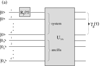
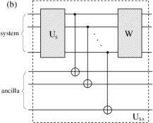
Figure 1: Quantum circuit implementing the geodesic evolution. (a): General circuit for a $d$-qubit system; $R_{y}(\tau)=e^{-{\rm{i}}\tau\sigma_{y}}$ is a rotation around the $y$-axis and $U_{{\sf S}{\sf A}}$ a system-ancilla entangling unitary satisfying (7). (b), (c): examples of quantum circuits for $U_{{\sf S}{\sf A}}$; the unitaries $W$, $U_{\sf S}$, and $U_{\sf A}$ are such that $U_{i}|0\rangle_{i}=\sum_{k}\sqrt{p_{k}}|k\rangle_{i}$, $i={\sf S},{\sf A}$, $U_{\sf S}|1\rangle_{\sf S}=\sum_{k}\alpha_{k}|k\rangle$ with $\alpha_{k}\in{\mathbb{R}}$, and $W|k\rangle_{\sf S}=|w_{k}\rangle_{\sf S}$, $k=0,\ldots,2^{d}-1$, where $\sqrt{p_{k}}$ and $\{|w_{k}\rangle\}$ are the coefficients and orthonormal basis in the Schmidt decomposition of $|\Psi\rangle$.

II.3 Optimality of geodesics for parameter estimation in open quantum systems

Before explaining our results, let us introduce some basic background on quantum metrology for readers not familiar with this field.

Parameter estimation in closed and open quantum systems.

The goal of parameter estimation is to estimate an unknown real parameter $x$ pertaining to an interval $X\subset{\mathbb{R}}$ by performing measurements on a quantum system (probe). Before each measurement, the system undergoes a $x$-dependent process transforming the input state $\rho_{{\rm in}}$ into an output state $\rho_{x}$. The estimator $x_{\rm est}\in X$ is a function of the measurement outcomes. The precision of the estimation is characterized by the variance $(\Delta x)^{2}=\langle(x_{\rm est}-x)^{2}\rangle_{x}$, where $\langle\cdot\rangle_{x}$ refers to the average over the outcomes conditioned to the parameter value $x$. Hereafter, we assume that the estimator is unbiased, i.e., $\langle x_{\rm est}\rangle_{x}=x$ and $\partial_{x}\langle x_{\rm est}\rangle_{x}=1$. If one performs $N_{\rm meas}$ independent identical measurements on identical probes prepared in state $\rho_{x}$, then the estimation error satisfies the quantum Crámer-Rao bound Helstrom68 ; Braunstein94

$$\Delta x\geq(\Delta x)_{\rm{best}}=\frac{1}{\sqrt{N_{\rm meas}\,{\cal F}_{Q}(x,\{\rho_{x}\}_{x\in X})}}\;,$$ (10)

where ${\cal F}_{Q}(x,\{\rho_{x}\}_{x\in X})$ is the quantum Fisher information (QFI). The QFI is obtained by maximizing over all measurements the classical Fisher information (CFI)

$${\cal F}_{\rm clas}(x,\{p_{j|x}\}_{x\in X})=\sum_{j,p_{j|x}>0}\frac{(\partial_{x}p_{j|x})^{2}}{p_{j|x}}\;,$$ (11)

where $p_{j|x}$ is the probability of the measurement outcome $j$ given that the system is in state $\rho_{x}$. Note that the QFI and CFI depend on general on the parameter value $x$. For clarity we write this dependence on $x$ explicitly. The bound (10) is saturated asymptotically (in the limit $N_{\rm meas}\gg 1$) by choosing: (i) the maximum likelihood estimator $x_{\rm est}$ (ii) the optimal measurement maximizing the CFI, for which ${\cal F}_{\rm clas}={\cal F}_{Q}$. This means that the right-hand side  of (10) gives the smallest error that can be achieved in the estimation. Using classical resources, this error scales with the number of probes $N$ like $1/\sqrt{N}$ (shot noise limit). Entanglement among the quantum probes can enhance the precision by a factor $1/\sqrt{N}$, leading to errors $(\Delta x)_{\rm{best}}$ scaling like $1/N$ (Heisenberg limit).

For a closed system in a pure state undergoing the $x$-dependent unitary transformation $|\Psi_{x}\rangle=e^{-{\rm{i}}xH}|\Psi_{\rm in}\rangle$, where $H$ is a given observable, the QFI is given by myreview ; Braunstein94

$${\cal F}_{Q}(\{|\Psi_{x}\}_{x\in X})\rangle = 4\big{(}\|\dot{\Psi}_{x}\|^{2}-\big{|}\langle\Psi_{x}|\dot{\Psi}_{x}\rangle\big{|}^{2}\big{)}$$ (12)

$$= 4\langle(\Delta H)^{2}\rangle_{\Psi_{\rm in}}\;,$$

where $|\dot{\Psi}_{x}\rangle$ is the derivative of $|\Psi_{x}\rangle$ with respect to $x$ and $\langle(\Delta H)^{2}\rangle_{\Psi}=\langle\Psi|H^{2}|\Psi\rangle-\langle\Psi|H|\Psi\rangle^{2}$ is the square quantum fluctuation of $H$ in state $|\Psi\rangle$. The input states maximizing this fluctuation are the superpositions

$$|\Psi_{\rm in}\rangle=\frac{1}{\sqrt{2}}\Big{(}|\epsilon_{\rm max}\rangle+e^{{\rm{i}}\varphi}|\epsilon_{\rm min}\rangle\Big{)}\;,$$ (13)

where $\varphi$ is a real phase and $|\epsilon_{\rm max}\rangle$ (respectively $|\epsilon_{\rm min}\rangle$) is an eigenstate of $H$ with maximal (minimal) eigenvalue $\epsilon_{\rm max}$ ($\epsilon_{\rm min}$). (We assume here that these eigenvalues are non-degenerated.) According to (10) and (12), the states (13) are the optimal input states minimizing the best estimation error $(\Delta x)_{\rm{best}}$. Indeed, by convexity of the QFI, using mixed input states $\rho_{{\rm in}}$ can not lead to smaller errors. Note that the QFI (12) is independent of $x$, as clear from the last expression. For this reason, we omit here $x$ in the argument of ${\cal F}_{Q}$. In contrast, for non-unitary evolutions the QFI depends in general upon the value $x$ of the estimated parameter.

For $N$ probes undergoing a unitary “parallel” transformation with the observable $H_{N}=\sum_{i=1}^{N}H_{i}$, where $H_{i}$ stands for the action of $H$ on the $i$th probe, the error has the Heisenberg scaling $(\Delta x)_{\rm{best}}\propto 1/N$ (more precisely, $(\Delta x)_{\rm{best}}=(2N\Delta\sqrt{N_{\rm meas}})^{-1}$ with $\Delta=(\epsilon_{\rm max}-\epsilon_{\rm min})/2$). The optimal input states, given by replacing $|\epsilon_{\rm max}\rangle$ and $|\epsilon_{\rm min}\rangle$ in (13) by the eigenvectors of $H_{N}$ associated to the maximal and minimal eigenvalues $N\epsilon_{\rm max}$ and $N\epsilon_{\rm min}$, are highly entangled.

In experimental setups, the coupling of the probes with their environment can not be neglected. A general description of the state transformation process is given by a family $\{{\cal M}_{x}\}_{x\in X}$ of $x$-dependent quantum channels, which account for the joint effects of the free evolutions of the probe ${\sf P}$ and environment ${\sf E}$ and the coupling between them. The probe output state is related to the input state $\rho_{\rm in}$ by

$$\rho_{x}={\cal M}_{x}(\rho_{\rm in})\;.$$ (14)

In a realistic scenario, measurements can be performed on the probe only, i.e., one can not extract information from the environment. An issue of current interest is to find optimal families of quantum channels $\{{\cal M}_{x}\}_{x\in X}$ and input states $\rho_{\rm in}$ which lead to the smallest error, i.e., to the largest possible QFI. The precision $(\Delta x)_{\rm{best}}$ can clearly not be smaller than the best precision $(\Delta x)_{\rm{best,{\sf P}{\sf E}}}$ which would be obtained from joint measurements on the probe and environment. A natural question is whether there exists a family of quantum channels such that $(\Delta x)_{\rm{best}}=(\Delta x)_{\rm{best,{\sf P}{\sf E}}}$ for any value of $x$. This means that the environment does not carry any information about the parameter $x$.

Figure 2: Quantum circuit implementing a geodesic transformation for the estimation of a phase shift $x$, with an error reaching the Heisenberg scaling. The single qubit unitaries $R_{y}$, $U_{\sf A}$ and $W$ are as in Fig. 1 with $d=1$. In spite of the presence of the C-NOT gates entangling the probe qubits with the ancilla qubits, the maximal information on $x$ can be recovered from measurements on the probe qubits only, with a minimal error $(\Delta x)_{\rm best}=(2N\Delta\sqrt{N_{\rm meas}})^{-1}$.

Optimality of geodesics in parameter estimation.

We will show in Sec. VI below that it is possible to find such a family of quantum channels and input state, which are moreover such that the error $(\Delta x)_{\rm{best}}$ is equal to the smallest possible error

$$(\Delta x)_{\rm{best}}=(\Delta x)_{\rm{best,{\sf P}{\sf E}}}=(2\Delta\sqrt{N_{\rm meas}})^{-1}\;,$$ (15)

where $\Delta=(\epsilon_{\rm max}-\epsilon_{\rm min})/2$ is as before the maximal quantum fluctuation of the observable $H$. Such a family is given by the CPTP maps associated to the Bures geodesics described in the previous subsection. The corresponding state transformation is

$$\rho_{x}=\gamma_{{\mathrm{g}}}(x\Delta)\;,$$ (16)

where $\gamma_{{\mathrm{g}}}(\tau)$ is a geodesic starting at

$$\gamma_{{\mathrm{g}}}(0)=\rho_{\rm in}=\operatorname{tr}_{\sf A}|\Psi_{\rm in}\rangle\langle\Psi_{\rm in}|$$ (17)

Note that the estimated parameter $x$ appears in (16) as a phase shift proportional to the dimensionless time $\tau$.

In other words, for the state transformation and phase shift $x$ given in (16), one has: (i) the precision on the estimation of $x$ obtained from measurements on the probe only is the same as that obtained by performing joint measurements on the probe and environment; (ii) the error $(\Delta x)_{\rm best}=(\Delta x)_{\rm{best,{\sf P}{\sf E}}}$ is the smallest achievable among all probe-environment initial states. Furthermore, as illustrated in Fig. 2, the error can reach the Heisenberg bound for a large number $N$ of entangled probes.

To justify properties (i)-(ii), let us look at the transformation (14) as resulting from the coupling of the probe with an ancilla ${\sf A}$, the probe and ancilla being initially in a pure state and undergoing a unitary transformation with some Hamiltonian $H$ acting on the probe and ancilla Hilbert space ${\cal K}={\cal H}\otimes{\cal H}_{\sf A}$. Note that this is always possible according to Stinepring’s theorem Stinespring55 . Thus

$$\rho_{x}=\operatorname{tr}_{\sf A}|\Psi_{x}\rangle\langle\Psi_{x}|\quad,\quad|\Psi_{x}\rangle=e^{-{\rm{i}}xH}|\Psi_{\rm in}\rangle\;.$$ (18)

Let us decompose the tangent vector $|\dot{\Psi}_{x}\rangle=\partial_{x}|\Psi_{x}\rangle$ into the sum of its horizontal part $|\dot{\Psi}^{\rm{h}}_{x}\rangle$ and its vertical part $|\dot{\Psi}^{\rm v}_{x}\rangle$ with $\langle\dot{\Psi}^{\rm{h}}_{x}|\dot{\Psi}^{\rm v}_{x}\rangle=0$, where horizontality means orthogonality to the orbit of $\rho_{x}$, see Fig. 3. According to the theory of Riemannian submersions, the norm of the horizontal part coincides with the square norm $(g_{\rm B})_{\rho_{x}}(\dot{\rho}_{x},\dot{\rho}_{x})$ of $\dot{\rho}_{x}=\partial_{x}\rho_{x}$, the latter norm being given by the Bures metric $g_{\rm B}$ at $\rho_{x}$ (see Sec. III). It is known that this square norm is equal to the QFI up to a factor of one fourth Braunstein94 ; myreview . Thus, thanks to Pythagorean theorem $\|\dot{\Psi}_{x}\|^{2}=\|\dot{\Psi}_{x}^{\rm{h}}\|^{2}+\|\dot{\Psi}_{x}^{\rm v}\|^{2}$, one obtains the following formula for the QFI of the probe

$${\cal F}_{Q}(x,\{\rho_{x}\}_{x\in X})={\cal F}_{Q}(\{|\Psi_{x}\rangle\}_{x\in X})-4\|\dot{\Psi}^{\rm v}_{x}\|^{2}\;,$$ (19)

where the QFI ${\cal F}(\{|\Psi_{x}\rangle\}_{x\in X})$ of the total system (probe and ancilla) is given by (12) and $\|\dot{\Psi}^{\rm v}_{x}\|^{2}$ quantifies the amount of information on $x$ in the ancilla. It follows that the equality ${\cal F}_{Q}(x,\{\rho_{x}\}_{x\in X})={\cal F}_{Q}(\{|\Psi_{x}\rangle\}_{x\in X})$ holds whenever $|\dot{\Psi}^{\rm v}_{x}\rangle=0$, that is, for horizontal tangent vectors $|\dot{\Psi}_{x}\rangle$.

Let $|\Psi_{\mathrm{g}}(\tau)\rangle$ be a pure state geodesic for the norm distance on ${\cal K}$. A general result on Riemannian submersions tells us that if the tangent vector $|\dot{\Psi}_{\mathrm{g}}(\tau)\rangle$ is horizontal at $\tau=0$ then it remains horizontal at all times $\tau$ and $|\Psi_{\mathrm{g}}(\tau)\rangle$ projects out to a geodesic $\gamma_{\mathrm{g}}(\tau)$ on ${\cal E}_{\cal H}$, where the projection corresponds here to the partial trace over the ancilla (see Sec. III.3 for more details). Therefore, for the state transformation (16) one has $|\dot{\Psi}_{x}^{\rm v}\rangle=0$ for all parameter values $x$. Thanks to (10) and (19), $(\Delta x)_{\rm{best}}$ is then equal to the best error obtained from measurements on the probe and ancilla. This justifies property (i) above. Furthermore, it is easy to show that $|\Psi_{\rm in}\rangle$ is the superposition (13) for the Hamiltonian $H=(\Delta)H_{{\rm{g}}}$, $H_{{\rm{g}}}$ being given by (3) with $|\Psi\rangle=|\Psi_{\rm in}\rangle$ and $|\dot{\Psi}\rangle=|\dot{\Psi}_{\rm in}\rangle/\|\dot{\Psi}_{\rm in}\|$. This justifies (ii).

We show in Sec. VI that, conversely, if (i) and (ii) hold then the state transformation has the form (16) for some geodesic $\gamma_{\mathrm{g}}$. Theorem 3 in this section characterizes all Hamiltonians $H$ and input states $|\Psi_{\rm in}\rangle$ satisfying the two following conditions, which are equivalent to (i) and (ii): (I) $|\dot{\Psi}_{x}\rangle$ is horizontal for all $x\in X$; (II) ${\cal F}(x,\{|\Psi_{x}\rangle\}_{x\in X})$ is maximal. We prove that these conditions hold if and only if $|\Psi_{x}\rangle=|\Psi_{\mathrm{g}}(x\Delta)\rangle=e^{-{\rm{i}}(x\Delta)H_{\mathrm{g}}}|\Psi_{\rm in}\rangle$ is a pure state geodesic of the probe and ancilla with a horizontal initial tangent vector $|\dot{\Psi}_{\rm in}\rangle$ satisfying (4). By the aforementioned result on Riemannian submersions, this means that (16) and (17) hold. Equivalently, (I) and (II) are satisfied if and only if $|\dot{\Psi}_{\rm in}\rangle=-{\rm{i}}(H-\langle H\rangle_{\Psi_{\rm in}})|\Psi_{\rm in}\rangle$ is horizontal and the restriction of $H$ to the two-dimensional subspace spanned by its eigenvectors associated to the maximal and minimal eigenvalues coincides up to a factor of $\Delta$ with the geodesic Hamiltonian (3) with $|\Psi\rangle=|\Psi_{\rm in}\rangle$ and $|\dot{\Psi}\rangle=|\dot{\Psi}_{\rm in}\rangle/\|\dot{\Psi}_{\rm in}\|$. Theorem 4 in Sec. VI shows that these eigenvectors must be related by $|\epsilon_{\rm min}\rangle=U\otimes{\mathds{1}}|\epsilon_{\rm max}\rangle$ for some local unitary $U$ acting on the probe.

Another nice property of the state transformation (16) is related to the optimal measurement. Recall that a measurement is given by a POVM $\{M_{j}\}$, that is, a set of non-negative operators $M_{j}\geq 0$ on ${\cal H}$ such that $\sum_{j}M_{j}={\mathds{1}}$. The outcome probabilities when the system is in state $\rho_{x}$ are given by $p_{j|x}=\operatorname{tr}M_{j}\rho_{x}$. An optimal measurement is a POVM $\{M_{j}^{\rm{opt}}\}$ for which the CFI (11) coincides with the QFI. Such a measurement leads to the smallest error $\Delta x=(\Delta x)_{\rm best}$ in (10). In general, $\{M_{j}^{\rm{opt}}\}$ depends on the parameter $x$ Caves96 . Since $x$ is unknown a priori, it is then in practice impossible to implement directly an optimal measurement strategy. A notable exception for which the optimal measurement is independent of $x$ is a closed system undergoing a unitary transformation with an input state given by the superposition (13) minimizing the error. Theorem 5 in Sec. VI shows that the geodesic transformation (16) enjoys the same property. More precisely, one has: (iii) there is an optimal POVM $\{M_{j}^{\rm{opt}}\}$ maximizing the CFI which is independent of $x$ and given by the von Neumann measurement with projectors onto $\ker\rho_{j}$, where $\rho_{j}$ are the states at which the geodesic $\gamma_{\mathrm{g}}$ intersects the boundary $\partial{\cal E}_{\cal H}$ of quantum states. This property gives a practical way to determine an optimal measurement in numerical simulations or experiments: first determine the smallest eigenvalue $p_{n}(x)=\min_{\|\psi\|=1}\langle\psi|\rho_{x}|\psi\rangle$ of $\rho_{x}$ for different values of $x$ until finding a parameter value $x_{j}$ such that $p_{n}(x_{j})\simeq 0$ (if $x$ is random and can not be tuned, just repeat the transformation many times); then determine all almost vanishing eigenvalues and the associated eigenvectors of $\rho_{j}=\rho_{x_{j}}$, e.g. by minimization of $\langle\psi|\rho_{j}|\psi\rangle$ in orthogonal subspaces or by using quantum state tomography; repeat this procedure for different values of $x$ until obtaining an orthonormal basis of ${\cal H}$ formed by eigenvectors of the states $\rho_{j}$ with vanishing eigenvalues (Theorem 6 in Appendix B shows that these eigenvectors indeed form an orthonormal basis). Then such a basis is an optimal measurement basis for the estimation of $x$.

Let us stress that the geometric approach described in the following sections is not restricted to geodesic evolutions and provides a new method for studying parameter estimation in open quantum systems. Actually, the above arguments show that the estimation error is smaller when the tangent vectors $|\dot{\Psi}_{x}\rangle$ have smaller vertical components, see (19). This observation may be useful for designing new engineering reservoir techniques in order to increase precision in quantum metrology in the presence of losses and dephasing.

Figure 3: The manifold of quantum states ${\cal E}={\cal E}_{\cal H}$ is the projection $\pi({\cal S})$ of the manifold ${\cal S}$ of pure states on an enlarged Hilbert space ${\cal H}\otimes{\cal H}_{\sf A}$, where $\pi$ is the partial trace over ${\cal H}_{\sf A}$. The horizontal subspaces at $|\Psi\rangle$ and $|\Phi_{V}\rangle$ are orthogonal to the orbits $\pi^{-1}(\rho)$ and $\pi^{-1}(\sigma)$ (red lines). A geodesic in ${\cal S}$ joining $|\Psi\rangle$ to $|\Phi_{V}\rangle$ (plain black curve) with a horizontal initial tangent vector $|{\dot{\Psi}}^{\rm{h}}\rangle$ projects out to a geodesic $\gamma_{{\mathrm{g}},V}$ on ${\mathcal{E}}$ (green plain curve). In contrast, if the geodesic in ${\cal S}$ (blue dashed curve) has a non horizontal initial tangent vector, its projection (green dashed line) is not a geodesic on ${\cal E}$. The differential ${\rm{d}}\pi$ maps the horizontal tangent vector $|{\dot{\Psi}}^{\rm{h}}\rangle$ to a tangent vector $\dot{\rho}$ of $\gamma_{{\mathrm{g}},V}$ having the same length $\|\dot{\rho}\|=\|{\dot{\Psi}}^{\rm{h}}\|$. A non horizontal vector $|{\dot{\Psi}}\rangle$ is mapped by ${\rm{d}}\pi$ to a vector $\dot{\rho}$ with a smaller length, given by $\|\dot{\rho}\|^{2}=\|\dot{\Psi}\|^{2}-\|{\dot{\Psi}}^{\rm{v}}\|^{2}$, where $|{\dot{\Psi}}^{\rm{v}}\rangle$ is the vertical component of $|{\dot{\Psi}}\rangle$ (Pythagorean theorem).

III Mathematical preliminaries

In this section we describe the geometrical properties of the manifold of mixed states of a quantum system equipped with the Bures distance and introduce the notion of Riemannian submersions.

III.1 Riemannian geometry for quantum states and Bures distance.

Let us first recall some basic notions of Riemannian geometry. A metric on a smooth manifold ${\cal E}$ is a smooth map $g$ associating to each point $\rho\in{\cal E}$ a scalar product $g_{\rho}$ on the tangent space $T_{\rho}{\cal E}$ at $\rho$. A curve $\gamma$ on ${\cal E}$ joining two points $\rho$ and $\sigma$ is parametrized by a piecewise $C^{1}$ map $\gamma:t\in[t_{0},t_{1}]\mapsto\gamma(t)\in{\cal E}$ such that $\gamma(t_{0})=\rho$ and $\gamma(t_{1})=\sigma$. Its length $\ell(\gamma)$ is

$$\ell(\gamma)=\int_{\gamma}{\rm{d}}s=\int_{t_{0}}^{t_{1}}{\rm{d}}t\,\sqrt{g_{\gamma(t)}(\dot{\gamma}(t),\dot{\gamma}(t))}\;,$$ (20)

where $\dot{\gamma}(t)$ stands for the time derivative ${\rm{d}}\gamma/{\rm{d}}t$. A Riemannian distance $d$ on ${\cal E}$ can be associated to any metric $g$, defined as the infimum $d(\rho,\sigma)=\inf_{\gamma}\ell(\gamma)$ of the lengths of all curves $\gamma$ joining $\rho$ and $\sigma$. Such a distance is called the geodesic distance on $({\cal E},g)$. Curves $\gamma_{\mathrm{g}}$ with constant velocity minimizing the length locally are called geodesics. More precisely, $\gamma_{\mathrm{g}}:[t_{0},t_{1}]\rightarrow{\cal E}$ is a geodesic if (i) $g_{\gamma_{\mathrm{g}}(t)}(\dot{\gamma_{\mathrm{g}}}(t),\dot{\gamma_{\mathrm{g}}}(t))={\rm const.}$ and (ii) $\forall\;\,t\in(t_{0},t_{1})$, $\exists\;\delta>0$ such that $\ell(\gamma_{\mathrm{g}}|_{[t,t+\delta]})=d(\gamma_{\mathrm{g}}(t),\gamma_{\mathrm{g}}(t+\delta))$. In particular, if there is a geodesic $\gamma_{\mathrm{g}}$ with length $\ell(\gamma_{\mathrm{g}})=d(\rho,\sigma)$ minimizing the length globally, one says that $\gamma_{\mathrm{g}}$ is the shortest geodesic joining $\rho$ and $\sigma$.

Conversely, one can associate to a distance $d$ on ${\cal E}$ a metric $g$ if $d$ satisfies the following condition (we ignore here regularity assumptions): for any $\rho\in{\cal E}$ and $\dot{\rho}\in T_{\rho}{\cal E}$, the square distance between $\rho$ and $\rho+t\dot{\rho}$ behaves as $t\to 0$ as

$${\rm{d}}s^{2}=d(\rho,\rho+t\dot{\rho})^{2}=g_{\rho}(\dot{\rho},\dot{\rho})t^{2}+{\cal O}(t^{3})\;.$$ (21)

In quantum mechanics, states are represented by non-negative operators $\rho$ with unit trace from the Hilbert space ${\cal H}$ of the system into itself. We assume hereafter that ${\cal H}$ has finite dimension $n=\dim({\cal H})<\infty$ and denote by ${\cal E}_{\cal H}$ the set of all quantum states of a given system. The arccos Bures distance between two states $\rho$ and $\sigma$ is defined by Nielsen

$$d_{\rm B}(\rho,\sigma)=\arccos\sqrt{F(\rho,\sigma)}\;,$$ (22)

where

$$F(\rho,\sigma)=\Bigl{(}\operatorname{tr}|\sqrt{\sigma}\sqrt{\rho}|\Bigr{)}^{2}=\Bigl{(}\operatorname{tr}(\sqrt{\rho}\,\sigma\sqrt{\rho})^{\frac{1}{2}}\Bigr{)}^{2}$$ (23)

is the fidelity. The set of all invertible states,

$${\cal E}_{\cal H}^{\,\mathrm{inv}}=\big{\{}\rho:{\cal H}\to{\cal H},\;;\;\rho>0,\operatorname{tr}\rho=1\big{\}}\;,$$ (24)

equipped with the distance $d_{\rm B}$ forms a smooth open Riemannian manifold. Its boundary $\partial{\cal E}_{\cal H}$ consists of density matrices $\rho$ having at least one vanishing eigenvalue; for instance, pure states $\rho_{\psi}=|\psi\rangle\langle\psi|$ are on the boundary.

The tangent space at $\rho\in{\cal E}_{\cal H}^{\,\mathrm{inv}}$ can be identified with the (real) vector space of self-adjoint traceless operators on ${\cal H}$,

$$T_{\rho}\,{\cal E}_{\cal H}=\big{\{}\dot{\rho}:{\cal H}\to{\cal H}\;,\;\dot{\rho}^{\dagger}=\dot{\rho}\;,\;\operatorname{tr}\dot{\rho}=0\big{\}}\;.$$ (25)

The metric $g_{\rm B}$ associated to the distance ${d}_{\rm B}$ is given explicitly by Hubner92 ; myreview

$$(g_{\rm B})_{\rho}(\dot{\rho},\dot{\sigma})={\frac{1}{2}}\mathrm{Re}\,\!\sum_{k,l=1}^{n}\frac{\overline{\langle k|\dot{\rho}|l\rangle}\langle k|\dot{\sigma}|l\rangle}{p_{k}+p_{l}}\;,\;\dot{\rho},\dot{\sigma}\in T_{\rho}\,{\cal E}_{\cal H}\;,$$ (26)

where $\{|k\rangle\}_{k=1}^{n}$ is an orthonormal basis of eigenvectors of $\rho$ with eigenvalues $p_{k}$. Note that $(g_{B})_{\rho}$ is well defined for invertible states $\rho$ only, i.e., when $p_{k}>0$ for all $k=1,\ldots,n$.

III.2 Purifications and smooth submersions

Mixed quantum states of a given system can be described by introducing an auxiliary system ${\sf A}$, called the ancilla, and viewing the system state $\rho$ as the reduced state of the system + ancilla. The dimension of the ancilla Hilbert space ${\cal H}_{\sf A}$ is assumed to fulfill $n_{\sf A}\geq n$. We denote by ${\cal K}={\cal H}\otimes{\cal H}_{\sf A}$ the Hilbert space of the composite system. A purification of $\rho$ on ${\cal K}$ is a pure state $|\Psi\rangle\langle\Psi|$ such that $|\Psi\rangle\in{\cal K}$ and $\rho=\pi(|\Psi\rangle)$, with

$$\pi(|\Psi\rangle)=\operatorname{tr}_{\sf A}|\Psi\rangle\langle\Psi|\;,$$ (27)

where $\operatorname{tr}_{\sf A}$ stands for the partial trace over the ancilla space ${\cal H}_{\sf A}$. For our purpose, it is convenient to consider purifications given by normalized vectors in $|\Psi\rangle\in{\cal K}$, instead of pure states (recall that a pure state is a normalized vector modulo a phase factor and can be represented as a rank-one projector $|\Psi\rangle\langle\Psi|$ in the projective space $P{\cal K}$). The condition $\rho>0$ is satisfied if and only if $|\Psi\rangle$ has Schmidt decomposition

$$|\Psi\rangle=\sum_{k=1}^{n}\sqrt{p_{k}}|k\rangle|\alpha_{k}\rangle$$ (28)

with $n$ positive Schmidt coefficients $\sqrt{p_{k}}>0$, $k=1,\ldots,n$. Here, $\{|\alpha_{k}\rangle\}_{k=1}^{n_{\sf A}}$ is an arbitrary orthonormal basis  of ${\cal H}_{\sf A}$. The set of purifications of invertible states is thus the subset

$${\cal S}_{{\cal K}}^{\,\mathrm{inv}} = \big{\{}|\Psi\rangle\in{\cal K}\;;\;\|\Psi\|=1\;,\;|\Psi\rangle\text{ has $n$ positive}$$ (29)

$$\qquad\text{Schmidt coefficients}\big{\}}$$

of the unit sphere in ${\cal K}$. The tangent space at $|\Psi\rangle\in{\cal S}_{\cal K}^{\,\mathrm{inv}}$ is

$$T_{|\Psi\rangle}{\cal S}_{{\cal K}}=\big{\{}|\dot{\Psi}\rangle\in{\cal K}\;;\;\mathrm{Re}\,\langle\Psi|\dot{\Psi}\rangle=0\big{\}}\;.$$ (30)

A natural metric on ${\cal S}_{{\cal K}}^{\,\mathrm{inv}}$ is $g_{\cal S}(|\dot{\Psi}\rangle,|\dot{\Phi}\rangle)=\mathrm{Re}\,\langle\dot{\Psi}|\dot{\Phi}\rangle$ (note that the scalar product is independent on $|\Psi\rangle$). This metric is that induced by the euclidean metric on ${\cal K}$. The Riemannian manifold $({\cal S}_{{\cal K}}^{\,\mathrm{inv}},g_{\cal S})$ is isometric under the action $|\Psi\rangle\mapsto{\mathds{1}}\otimes U_{\sf A}|\Psi\rangle$ of the unitary group $U(n_{\sf A})$ acting on the ancilla, that is,

$$g_{\cal S}({\mathds{1}}\otimes U_{\sf A}|\dot{\Psi}\rangle,{\mathds{1}}\otimes U_{\sf A}|\dot{\Phi}\rangle)=g_{\cal S}(|\dot{\Psi}\rangle,|\dot{\Phi}\rangle)$$ (31)

for any unitary $U_{\sf A}$ on ${\cal H}_{\sf A}$.

We now argue that ${\cal E}_{\cal H}^{\,\mathrm{inv}}$ can be viewed as the quotient of ${\cal S}_{{\cal K}}^{\,\mathrm{inv}}$ by the unitary group $U(n_{\sf A})$. The map (27) defines a projection from ${\cal S}_{{\cal K}}^{\,\mathrm{inv}}$ onto ${\cal E}_{\cal H}^{\,\mathrm{inv}}$. The set $\pi^{-1}(\rho)$ of all purifications of $\rho$ coincides with the orbit of $\rho$ under the group action,

$$\pi^{-1}(\rho)=\big{\{}|\Psi\rangle={\mathds{1}}\otimes U_{\sf A}|\Psi_{0}\rangle\;;\;U_{\sf A}\text{ unitary on }{\cal H}_{\sf A}\big{\}}\;,$$ (32)

where $|\Psi_{0}\rangle\in{\cal S}_{\cal K}^{\,\mathrm{inv}}$ is some fixed purification. This can be proven by noting that any purification of $\rho$ has the form (28); thus it can be obtained by applying a local unitary ${\mathds{1}}\otimes U_{\sf A}$ on $|\Psi_{0}\rangle$. Therefore, ${\cal E}_{\cal H}^{\,\mathrm{inv}}$ can be identified with the quotient manifold ${\cal S}^{\,\mathrm{inv}}_{{\cal K}}/U(n_{\sf A})$ and $\pi$ is the quotient map.

An important fact about $\pi$ is that its differentials ${\rm{d}}\pi|_{|\Psi\rangle}:T_{|\Psi\rangle}{\cal S}_{{\cal K}}\to T_{\rho}\,{\cal E}_{\cal H}$ are surjective for any $|\Psi\rangle\in{\cal S}_{\cal K}^{\,\mathrm{inv}}$. Such quotient maps with surjective differentials are called smooth submersions. The differential of the map (27) is given by

$${\rm{d}}\pi|_{|\Psi\rangle}(|\dot{\Psi}\rangle)=\operatorname{tr}_{\sf A}(|\Psi\rangle\langle\dot{\Psi}|+|\dot{\Psi}\rangle\langle\Psi|)\;.$$ (33)

To prove that $\pi:{\cal S}_{\cal K}^{\,\mathrm{inv}}\to{\cal E}_{\cal H}^{\,\mathrm{inv}}$ is a smooth submersion, let us first note that for any fixed $\dot{\rho}\in T_{\rho}{\cal E}_{\cal H}$, if $|\dot{\Psi}\rangle\in{\cal K}$ satisfies

$${\rm{d}}\pi|_{|\Psi\rangle}(|\dot{\Psi}\rangle)=\dot{\rho}$$ (34)

then $|\dot{\Psi}\rangle\in T_{|\Psi\rangle}{\cal S}_{{\cal K}}$. In fact, by taking the trace of the right hand sides of (33) and (34) one gets $2\mathrm{Re}\,\langle\Psi|\dot{\Psi}\rangle=\operatorname{tr}\dot{\rho}=0$. Setting $\rho=\pi(|\Psi\rangle)$, it is easy to check that $|\dot{\Psi}\rangle={\frac{1}{2}}\dot{\rho}\rho^{-1}\otimes{\mathds{1}}|\Psi\rangle$ is a solution of (34). Hence ${\rm{d}}\pi|_{|\Psi\rangle}$ is surjective. Let us point out that this is not true if $\pi$ is defined on the whole unit sphere ${\cal S}_{\cal K}$ of ${\cal K}$, instead of ${\cal S}_{\cal K}^{\,\mathrm{inv}}$, i.e., if one adds to ${\cal E}_{\cal H}^{\,\mathrm{inv}}$ its boundary $\partial{\cal E}_{\cal H}$.

III.3 Riemannian submersions

Our results in this paper rely on the notion of Riemannian submersion. In this subsection we review the properties of such submersions (see e.g. Gallot_book for more details) and show that the partial trace (27) is an instance of Riemannian submersion ${\cal S}_{\cal K}^{\,\mathrm{inv}}\to{\cal E}_{\cal H}^{\,\mathrm{inv}}$.

Let $\pi:{\cal X}\to{\cal E}$ be a smooth submersion, where ${\cal X}$ is a Riemannian manifold with metric $g_{\cal X}$. The tangent space $T_{\psi}{\cal X}$ at $\psi\in{\cal X}$ can be decomposed into a direct sum of two orthogonal subspaces ${\mathfrak{v}}_{\psi}=\ker({\rm{d}}\pi|_{\psi})$ and ${\mathfrak{h}}_{\psi}={\mathfrak{v}}_{\psi}^{\bot}$, called respectively the vertical and horizontal subspaces (orthogonality is for the scalar product $(g_{\cal X})_{\psi}$). It can be shown that there exists a unique Riemannian metric $g_{\cal E}$ on the quotient manifold ${\cal E}$ such that for all $\psi\in{\cal X}$, the restriction of ${\rm{d}}\pi|_{\psi}$ to the horizontal subspace $\mathfrak{h}_{\psi}$ is an isometry from $({\mathfrak{h}}_{\psi},(g_{\cal X})_{\psi})$ to $(T_{\rho}{\cal E},(g_{\cal E})_{\rho})$, with $\rho=\pi(\psi)$. One then says that $\pi:({\cal X},g_{\cal X})\rightarrow({\cal E},g_{\cal E})$ is a Riemannian submersion. It is not difficult to prove that $g_{\cal E}$ is associated to the distance $d_{\cal E}$ on ${\cal E}$ defined by

$$d_{{\cal E}}(\rho,\sigma)=\inf_{\phi\in\pi^{-1}(\sigma)}d_{\cal X}(\psi_{1},\phi)\;,$$ (35)

where $d_{\cal X}$ is a distance having the metric $g_{\cal X}$ and $\psi_{1}$ is an arbitrary (fixed) point on the orbit of $\rho$.

A nice property of Riemannian submersions is that the geodesics on the quotient space ${\cal E}$ can be obtained by projecting certain geodesics on ${\cal X}$. More precisely, for any geodesic $\Gamma:[t_{0},t_{1}]\to{\cal X}$ on $({\cal X},g_{\cal X})$ such that $\dot{\Gamma}(0)\in{\mathfrak{h}}_{\Gamma(0)}$, one has Gallot_book :

• $\dot{\Gamma}(t)\in{{\mathfrak{h}}}_{\Gamma(t)}$ for any $t\in[t_{0},t_{1}]$;

• $\gamma=\pi\circ\Gamma$ is a geodesic on $({\cal E},g_{\cal E})$.

Conversely, any geodesic $\gamma$ on $({\cal E},g_{\cal E})$ with $\gamma(0)=\rho$ can be lifted locally to an arc of geodesic $\Gamma$ on $({\cal X},g_{\cal X})$ with horizontal tangent vectors such that $\Gamma(0)=\psi$, for any $\psi\in\pi^{-1}(\rho)$. This property is illustrated in Fig. 3. We will call horizontal geodesics the geodesics $\Gamma$ on ${\cal X}$ such that $\dot{\Gamma}(0)\in{\mathfrak{h}}_{\Gamma(0)}$.

Let us apply this formalism to the smooth submersion $\pi$ given by (27). A natural distance on ${\cal S}_{\cal K}^{\,\mathrm{inv}}$ having the metric $g_{\cal S}$ is the norm distance $d_{\cal S}(|\Psi\rangle,|\Phi\rangle)=\||\Psi\rangle-|\Phi\rangle\|$. The metric on ${\cal E}_{\cal H}^{\,\mathrm{inv}}$ which makes $\pi$ a Riemannian submersion turns out to be the Bures metric $g_{B}$. This can be seen by invoking Uhlmann’s theorem, which states that Nielsen ; Uhlmann76

$$d_{\rm B}(\rho,\sigma)=\min_{|\Psi\rangle\in\pi^{-1}(\rho),|\Phi\rangle\in\pi^{-1}(\sigma)}\arccos\big{|}\langle\Psi|\Phi\rangle\big{|}\;,$$ (36)

where in the right-hand side  the arccos distance between pure states is minimized. Equivalently, the Bures distance ${d}_{\rm{Bures}}(\rho,\sigma)=2\sin(d_{\rm B}(\rho,\sigma)/2))$ is given by Uhlmann86 ; myreview

$${d}_{\rm{Bures}}(\rho,\sigma) = \bigl{(}2-2\sqrt{F(\rho,\sigma)}\bigr{)}^{\frac{1}{2}}$$ (37)

$$= \min_{|\Psi\rangle\in\pi^{-1}(\rho),|\Phi\rangle\in\pi^{-1}(\sigma)}\big{\|}|\Psi\rangle-|\Phi\rangle\big{\|}\;.$$

Note that the two distances $d_{\rm B}$ and $d_{\rm{Bures}}$ have the same metric $g_{\rm B}$, given by (26). Eqs. (36) and (37) tell us that the arccos and Bures distances between $\rho$ and $\sigma$ are the minimal distances between the two orbits of $\rho$ and $\sigma$. By (32) and the unitary invariance of the scalar product in ${\cal K}$, the minima in these equations can be carried out over all $|\Phi\rangle\in\pi^{-1}(\sigma)$ for some fixed $|\Psi_{1}\rangle\in\pi^{-1}(\rho)$. Thus $d_{\rm{Bures}}$ has the form (35) with $d_{\cal X}=d_{\cal S}$.

Let us end this subsection by determining the vertical and horizontal subspaces in the case of the purification manifold ${\cal X}={\cal S}_{\cal K}^{\,\mathrm{inv}}$ and quotient map (27). To determine ${\mathfrak{v}}_{|\Psi\rangle}=\ker({\rm{d}}\pi|_{|\Psi\rangle})$, we observe that curves contained in the orbit $\pi^{-1}(\rho)$ have by definition vertical tangent vectors. Conversely, for a smooth curve $t\mapsto|\Psi(t)\rangle$ with a vertical tangent vector $|\dot{\Psi}\rangle$ at $t=0$, it holds $|\Psi(t)\rangle=|\Psi_{\rm{v}}(t)\rangle+{\cal O}(t^{2})$ with $t\mapsto|\Psi_{\rm{v}}(t)\rangle={\mathds{1}}\otimes U_{\sf A}(t)|\Psi\rangle$ a curve in $\pi^{-1}(\rho)$ and $U_{\sf A}(t)$ a time-dependent unitary ancilla operator. Thus, using $\dot{U}_{\sf A}U_{\sf A}^{\dagger}=-U_{\sf A}\dot{U}_{\sf A}^{\dagger}$, one has

$${\mathfrak{v}}_{|\Psi\rangle}=\big{\{}{\mathds{1}}\otimes K_{\sf A}|\Psi\rangle\;;\;K_{\sf A}\text{ skew Hermitian}\big{\}}\;.$$ (38)

In order to obtain the horizontal subspace ${\mathfrak{h}}_{|\Psi\rangle}={\mathfrak{v}}_{|\Psi\rangle}^{\bot}$, we use the Schmidt decomposition (28) and expand an arbitrary horizontal tangent vector $|\dot{\Psi}^{\rm{h}}\rangle=\sum_{k,l}c_{kl}|k\rangle|\alpha_{l}\rangle$ in the product basis $\{|k\rangle|\alpha_{l}\rangle\}_{k,l=1}^{n,n_{\sf A}}$. Since $|\dot{\Psi}^{\rm{h}}\rangle$ is orthogonal to ${\mathfrak{v}}_{|\Psi\rangle}$, one finds

$$0 = \mathrm{Re}\,\langle\dot{\Psi}^{\rm{h}}|{\mathds{1}}\otimes K_{\sf A}|\Psi\rangle$$

$$= \sum_{k=1}^{n}\sum_{l=1}^{n_{\sf A}}\big{(}\overline{c}_{kl}\sqrt{p_{k}}\langle\alpha_{l}|K_{\sf A}|\alpha_{k}\rangle-c_{kl}\sqrt{p_{k}}\langle\alpha_{k}|K_{\sf A}|\alpha_{l}\rangle\big{)}$$

for any skew Hermitian ancilla operator $K_{\sf A}$. Choosing $K_{\sf A}={\rm{i}}^{\,\nu}|\alpha_{l}\rangle\langle\alpha_{k}|-(-{\rm{i}})^{\nu}|\alpha_{k}\rangle\langle\alpha_{l}|$ with $\nu=0$ or $1$, this gives

$$c_{kl}\sqrt{p_{k}}=\begin{cases}\overline{c}_{lk}\sqrt{p_{l}}&\text{ if $1\leq k,l\leq n$}\\ 0&\text{ if $n<l\leq n_{\sf A}$.}\end{cases}$$ (40)

Let us set $H_{\sf S}=\sum_{k,l=1}^{n}h_{kl}|k\rangle\langle l|$ with $h_{kl}=c_{kl}p_{l}^{-{\frac{1}{2}}}$. It follows from (40) that $H_{\sf S}=H^{\dagger}_{\sf S}$. Furthermore,

$$|\dot{\Psi}^{\rm{h}}\rangle=\sum_{k,l=1}^{n}h_{kl}\sqrt{p_{l}}|k\rangle|\alpha_{l}\rangle=H_{\sf S}\otimes{\mathds{1}}_{\sf A}|\Psi\rangle\;.$$ (41)

Reciprocally, if $|\dot{\Psi}^{\rm{h}}\rangle=H_{\sf S}\otimes{\mathds{1}}_{\sf A}|\Psi\rangle$ with $H_{\sf S}$ self-adjoint then $\mathrm{Re}\,\langle\dot{\Psi}^{\rm{h}}|{\mathds{1}}\otimes K_{\sf A}|\Psi\rangle=0$. The condition $\mathrm{Re}\,\langle\dot{\Psi}^{\rm{h}}|\Psi\rangle=0$ coming from the requirement that $|\dot{\Psi}^{\rm{h}}\rangle$ is in the tangent space (30) yields the additional constraint $\langle H_{\sf S}\otimes{\mathds{1}}_{\sf A}\rangle_{\Psi}=0$. Thus

$${\mathfrak{h}}_{|\Psi\rangle}=\big{\{}H_{\sf S}\otimes{\mathds{1}}_{\sf A}|\Psi\rangle\,;\,H_{\sf S}\text{ self-adjoint, }\langle H_{\sf S}\otimes{\mathds{1}}_{\sf A}\rangle_{\Psi}=0\big{\}}\,.$$ (42)

In conclusion, we have shown that the partial trace map (27) defines a Riemannian submersion from ${\cal S}_{\cal K}^{\,\mathrm{inv}}$ equipped with the metric $g_{\cal S}$ to the manifold ${\cal E}_{\cal H}^{\,\mathrm{inv}}$ equipped with the Bures metric $g_{\rm B}$. This means that ${\rm{d}}\pi$ is an isometry from $({\mathfrak{h}}_{|\Psi\rangle},g_{\cal S})$ to $(T_{\rho}\,{\cal E}_{\cal H},g_{\rm B})$, namely,

$$(g_{\rm B})_{\rho}\big{(}{\rm{d}}\pi|_{|\Psi\rangle}(|\dot{\Psi}^{\rm{h}}\rangle),{\rm{d}}\pi|_{|\Psi\rangle}(|\dot{\Phi}^{\rm{h}}\rangle)\big{)}=\mathrm{Re}\,\langle\dot{\Psi}^{\rm{h}}|\dot{\Phi}^{\rm{h}}\rangle$$ (43)

for any purification $|\Psi\rangle$ of $\rho$ and any horizontal tangent vectors $|\dot{\Psi}^{\rm{h}}\rangle,|\dot{\Phi}^{\rm{h}}\rangle\in{\mathfrak{h}}_{|\Psi\rangle}$.

IV Bures geodesics

IV.1 Determination of the geodesics

We determine in this subsection the Bures geodesics by applying the mathematical framework of the preceding section (see Bhatia_17 for a similar approach in the case of the space of positive definite matrices, i.e., unnormalized quantum states).

The shortest geodesic joining two vectors $|\Psi\rangle$ and $|\Phi\rangle$ on the unit sphere ${\cal S}_{\cal K}^{\,\mathrm{inv}}$ equipped with the metric $g_{\cal S}$ is the arc of great circle

$$|\Psi_{\mathrm{g}}(\tau)\rangle=\cos\tau\,|\Psi\rangle+\sin\tau\,|\dot{\Psi}\rangle\quad,\quad 0\leq\tau\leq\theta\;,$$ (44)

where $|\dot{\Psi}\rangle\in T_{|\Psi\rangle}{\cal S}_{\cal K}^{\,\mathrm{inv}}$ and $\theta=\arccos(\mathrm{Re}\,\langle\Psi|\Phi\rangle)$ is the angle between $|\Psi\rangle$ and $|\Phi\rangle$. We may assume without loss of generality that $\theta\not=0,\pi$, since otherwise $|\Psi\rangle$ and $|\Phi\rangle=\pm|\Psi\rangle$ project out to the same state $\rho=\sigma$. The longest arc of great circle joining $|\Psi\rangle$ and $|\Phi\rangle$ needs not to be considered here, because it is the extension of the shortest geodesic joining $|\Psi\rangle$ and $-|\Phi\rangle$ and the latter vector belongs to the same orbit as $|\Phi\rangle$. The geodesic tangent vector at $\tau=0$ is given by

$$|\dot{\Psi}_{\mathrm{g}}(0)\rangle=|\dot{\Psi}\rangle=\frac{1}{\sin\theta}\big{(}|\Phi\rangle-\cos\theta|\Psi\rangle\big{)}\;.$$ (45)

It is easy to check on this formula that $\|\dot{\Psi}\|=1$, i.e., the geodesic (44) has unit velocity.

According to the properties of Riemannian submersions (Sec. III.3), the Bures geodesics joining the invertible states $\rho=\pi(|\Psi\rangle)$ and $\sigma=\pi(|\Phi\rangle)$ are obtained by projecting the arcs of big circle (44) having horizontal tangent vectors $|\dot{\Psi}\rangle\in{\mathfrak{h}}_{\Psi}$. Let us consider the purification of $\rho$ given by

$$|\Psi\rangle=\sqrt{\rho}\otimes{\mathds{1}}_{\sf A}\sum_{k=1}^{n}|k\rangle|\alpha_{k}\rangle\;,$$ (46)

where we have used the Schmidt decomposition (28). The last sum is an (unnormalized) maximally entangled state of the system and ancilla. Similarly, by (32) any purification of $\sigma$ has the form $|\Phi\rangle=\sqrt{\sigma}\,W\rho^{-1/2}\otimes U_{\sf A}|\Psi\rangle$, where $W$ and $U_{\sf A}$ are two unitaries on ${\cal H}$ and ${\cal H}_{\sf A}$, respectively, with $\{W|k\rangle\}$ an eigenbasis of $\sigma$.

We have to determine the purifications $|\Phi\rangle$ of $\sigma$ such that the horizontality condition $|\dot{\Psi}\rangle\in{\mathfrak{h}}_{|\Psi\rangle}$ holds. In view of (42), (45), and (46), this condition can be written as

$$\frac{1}{\sin\theta}\bigg{(}\sqrt{\sigma}\,W\otimes U_{\sf A}-\cos\theta\sqrt{\rho}\otimes{\mathds{1}}_{\sf A}\bigg{)}\sum_{k=1}^{n}|k\rangle|\alpha_{k}\rangle$$

$$\qquad=H_{\sf S}\sqrt{\rho}\otimes{\mathds{1}}_{\sf A}\sum_{k=1}^{n}|k\rangle|\alpha_{k}\rangle\;.$$ (47)

for some self-adjoint operator $H_{\sf S}$ such that $\langle H_{\sf S}\otimes{\mathds{1}}_{\sf A}\rangle_{\Psi}=0$. In particular, one has $\langle\alpha_{l}|U_{\sf A}|\alpha_{k}\rangle=0$ for $n<l\leq n_{\sf A}$ and $1\leq k\leq n$. We now use the identity

$${\mathds{1}}\otimes U_{\sf A}\sum_{k=1}^{n}|k\rangle|\alpha_{k}\rangle=U_{\sf A}^{\rm T}\otimes{\mathds{1}}_{\sf A}\sum_{k=1}^{n}|k\rangle|\alpha_{k}\rangle\;,$$ (48)

where $U_{\sf A}^{\rm T}=\sum_{k,l=1}^{n}\langle\alpha_{l}|U_{\sf A}|\alpha_{k}\rangle|k\rangle\langle l|$ (when $n_{\sf A}>n$, (48) is true provided that ${\mathrm{span}}\{|\alpha_{1}\rangle,\ldots,|\alpha_{n}\rangle\}$ is invariant under $U_{\sf A}$, which is indeed the case here). Observe that $U_{\sf A}^{\rm T}$ and thus $U=WU_{\sf A}^{\rm T}$ are unitaries. Multiplying both members of (IV.1) by $\sqrt{\rho}$, one deduces that this equation is equivalent to

$$\frac{1}{\sin\theta}\bigg{(}\sqrt{\rho}\sqrt{\sigma}\,U-\cos\theta\,\,\rho\bigg{)}=\sqrt{\rho}\,H_{\sf S}\sqrt{\rho}\;.$$ (49)

Therefore, (IV.1) is equivalent to $\sqrt{\rho}\sqrt{\sigma}\,U$ being self-adjoint for some unitary $U$ on ${\cal H}$.

It is convenient at this point to introduce the polar decomposition

$$\sqrt{\sigma}\sqrt{\rho}=U_{\sigma\rho}\Lambda_{\sigma\rho}\;\;,\;\;\Lambda_{\sigma\rho}=|\sqrt{\sigma}\sqrt{\rho}|>0\;,$$ (50)

where $U_{\sigma\rho}$ is unitary. Let $V$ be the unitary operator given by $V=U_{\sigma\rho}^{\dagger}U$. Then $\sqrt{\rho}\sqrt{\sigma}\,U$ is self-adjoint if and only if $\Lambda_{\sigma\rho}V=V^{\dagger}\Lambda_{\sigma\rho}$. This implies $V^{\dagger}\Lambda^{2}_{\sigma\rho}V=\Lambda^{2}_{\sigma\rho}$, i.e., $V$ commutes with $\Lambda^{2}_{\sigma\rho}$ and thus with $\Lambda_{\sigma\rho}$. As a result, $V^{\dagger}\Lambda_{\sigma\rho}=V\Lambda_{\sigma\rho}$, which entails $V^{\dagger}=V$ (since $\Lambda_{\sigma\rho}>0$). Thus the horizontally condition (IV.1) holds if and only if $U=U_{\sigma\rho}V$ with $V$ unitary and self-adjoint, $V^{2}={\mathds{1}}$, and $V$ commutes with $\Lambda_{\sigma\rho}$. The corresponding purifications of $\sigma$ are

$$|\Phi_{V}\rangle = \sqrt{\sigma}\,U_{\sigma\rho}V\rho^{-1/2}\otimes{\mathds{1}}_{\sf A}|\Psi\rangle$$ (51)

$$= \rho^{-1/2}\Lambda_{\sigma\rho}V\rho^{-1/2}\otimes{\mathds{1}}_{\sf A}|\Psi\rangle\;.$$

Note that $\langle\Psi|\Phi_{V}\rangle$ is real. By (44) and (45), the horizontal geodesics on ${\cal S}_{\cal K}^{\,\mathrm{inv}}$ are given by

$$|\Psi_{{\mathrm{g}},V}(\tau)\rangle=\frac{1}{\sin\theta_{V}}\Big{(}\sin(\theta_{V}-\tau)|\Psi\rangle+\sin\tau|\Phi_{V}\rangle\Big{)}$$ (52)

with $\cos\theta_{V}=\langle\Psi|\Phi_{V}\rangle=\operatorname{tr}\Lambda_{\sigma\rho}V$. By using the identity

$$\operatorname{tr}_{\sf A}|\Phi_{V}\rangle\langle\Psi|=\sqrt{\sigma}\,U_{\sigma\rho}V\sqrt{\rho}=\rho^{-1/2}\Lambda_{\sigma\rho}V\sqrt{\rho}\;,$$ (53)

we obtain the geodesics $\gamma_{{\mathrm{g}},V}(\tau)=\pi(|\Psi_{{\mathrm{g}},V}(\tau)\rangle)$ on ${\cal E}_{\cal H}$, where $\pi$ is the quotient map (27),

$$\gamma_{{\mathrm{g}},V}(\tau)=\frac{1}{\sin^{2}\theta_{V}}\bigg{(}\sin^{2}(\theta_{V}-\tau)\,\rho+\sin^{2}(\tau)\,\sigma$$

$$+\sin(\theta_{V}-\tau)\sin(\tau)\Big{(}\rho^{-1/2}\Lambda_{\sigma\rho}V\rho^{1/2}+{\mathrm{h.c.}}\Big{)}\bigg{)}$$ (54)

with $0\leq\tau\leq\theta_{V}$. Eq. (IV.1) generalizes formula (1) of Sec. II. It coincides with this formula for $V={\mathds{1}}$. Thanks to (43) and to the horizontality of $|\dot{\Psi}_{V}\rangle$, $\gamma_{{\mathrm{g}},V}$ has unit square velocity $(g_{\rm B})_{\rho}(\dot{\gamma}_{{\mathrm{g}},V},\dot{\gamma}_{{\mathrm{g}},V})=\|\dot{\Psi}_{V}\|^{2}=1$. Thus $\theta_{V}=\ell(\gamma_{{\mathrm{g}},V})$ is the geodesic length.

The geodesic with the smallest length is obtained for $V={\mathds{1}}$. In fact, denoting by $\lambda_{k}>0$ and $v_{k}\in\{-1,1\}$ the eigenvalues of $\Lambda_{\rho\sigma}$ and $V$, one has

$$\cos\theta_{V}=\operatorname{tr}\Lambda_{\sigma\rho}V=\sum_{k=1}^{n}\lambda_{k}v_{k}$$

$$\quad\leq\sum_{k=1}^{n}\lambda_{k}=\operatorname{tr}\Lambda_{\sigma\rho}=\sqrt{F(\rho,\sigma)}=\cos\theta_{1}\;,$$ (55)

where we have set $\theta_{1}=\theta_{V={\mathds{1}}}$ and used $[V,\Lambda_{\sigma\rho}]=0$. Similarly, the longest geodesic joining $\rho$ to $\sigma$ is obtained by choosing $V=-{\mathds{1}}$ and has length $\pi-\theta_{1}$. In view of (51), such a geodesic is the projection of the arc of great circle joining $|\Psi\rangle$ and the vector $|\Phi_{-{\mathds{1}}}\rangle=-|\Phi_{{\mathds{1}}}\rangle$ diametrically opposite to $|\Phi_{\mathds{1}}\rangle$ on the sphere ${\cal S}^{\,\mathrm{inv}}_{\cal K}$. The latter is obtained by inverting time on the great circle through $|\Psi\rangle$ and $|\Phi_{\mathds{1}}\rangle$ and by replacing the arc length $\theta_{1}$ by $\pi-\theta_{1}$. Thus, by extending the shortest and longest geodesics $\gamma_{{\mathrm{g}},{\mathds{1}}}$ and $\gamma_{{\mathrm{g}},-{\mathds{1}}}$ joining $\rho$ and $\sigma$ to the interval $[0,\pi]$, one obtains the same closed curve albeit with opposite orientations. More generally, the pair of geodesics $(\gamma_{{\mathrm{g}},V},\gamma_{{\mathrm{g}},-V})$ enjoys the same property.

We have proven:

Theorem 1.

The Bures geodesics joining the two distinct invertible states $\rho$ and $\sigma\in{\cal E}_{\cal H}^{\,\mathrm{inv}}$ are given by

$$\gamma_{{\mathrm{g}},V}(\tau)=X_{\rho\sigma,V}(\tau)\,\rho\,X_{\rho\sigma,V}(\tau)\quad,\quad 0\leq\tau\leq\theta_{V}\;,$$ (56)

where the geodesic length $\theta_{V}$ is given by (IV.1), $X_{\rho\sigma,V}(\tau)$ is the operator defined by

$$X_{\rho\sigma,V}(\tau)=\frac{1}{\sin\theta_{V}}\Big{(}\sin(\tau)M_{\rho\sigma,V}+\sin(\theta_{V}-\tau){\mathds{1}}\Big{)}$$ (57)

with

$$M_{\rho\sigma,V}=\rho^{-1/2}|\sqrt{\sigma}\sqrt{\rho}|V\rho^{-1/2}\;,$$ (58)

and $V$ is an arbitrary unitary self-adjoint operator commuting with $\Lambda_{\sigma\rho}=|\sqrt{\sigma}\sqrt{\rho}|$. Furthermore, the geodesic with the smallest length, denoted hereafter by $\gamma_{\mathrm{g}}$, is obtained by choosing $V={\mathds{1}}$ in (56)-(58) and has length

$$\ell(\gamma_{\mathrm{g}})=\theta_{1}={d}_{\rm B}(\rho,\sigma)\;\in\;(0,\frac{\pi}{2}]\;.$$ (59)

The explicit form (56) of the Bures geodesics have been obtained in Refs. Barnum_thesis ; Ericson05 in the special case $V={\mathds{1}}$. Our derivation shows that, in addition to this shortest geodesic, there are other geodesics having larger lengths $\theta_{V}$, corresponding to $V\not={\mathds{1}}$. These geodesics will be classified below according to the number of time they intersect the boundary $\partial{\cal E}_{\cal H}$ between $\rho$ and $\sigma$. More precisely, there are $2^{n}$ geodesics joining two invertible states $\rho$ and $\sigma$ if $\Lambda_{\sigma\rho}$ has a non-degenerate spectrum. Actually, then there are $2^{n}$ choices for $V$ because $V$ is diagonal in an eigenbasis of $\Lambda_{\sigma\rho}$ (since $[\Lambda_{\sigma\rho},V]=0$) and thus it is fully characterized by its eigenvalues $v_{k}\in\{1,-1\}$. In contrast, if $\Lambda_{\sigma\rho}$ has a degenerate eigenvalue $\lambda_{k}$ then there are infinitely many geodesics $\gamma_{{\mathrm{g}},V}$ joining $\rho$ and $\sigma$, in analogy with what happens for diametrically opposite points on a sphere. In fact, in that case there are infinitely many choices for $V$ as $V_{k}=\Pi_{k}V\Pi_{k}$ can be any $r_{k}\times r_{k}$ self-adjoint unitary matrix, where $\Pi_{k}$ and $r_{k}$ are the eigenprojector and multiplicity of $\lambda_{k}$. Note that in all cases there are at most $2^{n}$ distinct geodesic lengths $\theta_{V}=\ell(\gamma_{{\mathrm{g}},V})$, since $\theta_{V}$ only depends on the spectrum of $V$, see (IV.1). The geodesic with the shortest length is always unique and obtained for $V={\mathds{1}}$. The second shortest geodesic length $\theta_{2}$ is given by $\cos\theta_{2}=\cos\theta_{1}-2\lambda_{\rm{min}}$, $\lambda_{\rm{min}}$ being the smallest eigenvalue of $\Lambda_{\sigma\rho}$. If $\lambda_{\rm{min}}$ is not degenerated, the corresponding geodesic is unique and obtained by choosing $V=V_{i_{\rm m}}$ such that it has a single negative eigenvalue $v_{i_{\rm m}}=-1$, with $\lambda_{i_{\rm m}}=\lambda_{\rm{min}}$.

One infers from (59) that the geodesic distance (obtained as the minimal length of curves joining $\rho$ and $\sigma$) is the arccos Bures distance ${d}_{\rm B}$, see (22). This is the main reason for using here that distance instead of the Bures distance (37); $d_{\rm B}(\rho,\sigma)$ is the angle $\theta_{1}=\arccos\langle\Psi|\Phi_{\mathds{1}}\rangle$ between the purification vectors $|\Psi\rangle$ and $|\Phi_{\mathds{1}}\rangle$ of $\rho$ and $\sigma$ (recall that $\langle\Psi|\Phi_{V}\rangle\in{\mathbb{R}}$). Hence $|\Phi_{\mathds{1}}\rangle$ (and similarly $|\Phi_{-{\mathds{1}}}\rangle=-|\Phi_{\mathds{1}}\rangle$) is a purification $|\Phi\rangle\in\pi^{-1}(\sigma)$ of $\sigma$ maximizing the pure state fidelity $|\langle\Psi|\Phi\rangle|$ in Uhlmann’s theorem $\sqrt{F(\rho,\sigma)}=\max_{|\Phi\rangle}|\langle\Psi|\Phi\rangle|$ Uhlmann76 ; Nielsen . This gives a way to compute numerically $|\Phi_{\pm{\mathds{1}}}\rangle$, and thus the horizontal geodesic (52), by using an optimization algorithm, instead of relying on the formula $|\Phi_{V}\rangle=M_{\rho\sigma,V}\otimes{\mathds{1}}_{\sf A}|\Psi\rangle$, which requires diagonalizing $\rho$ and $\sqrt{\sigma}\sqrt{\rho}$ to compute $M_{\rho\sigma,V}$. The purifications $|\Phi_{V}\rangle$ for $V\not=\pm{\mathds{1}}$ correspond to relative maxima of $|\langle\Psi|\Phi\rangle|$, which are smaller than the global maximum, see (IV.1).

The properties of the self-adjoint operators (58) are given in Appendix A. As pointed out in Ericson05 , for $V={\mathds{1}}$ this operator is related to the optimal measurement to discriminate the distributions of measurement outcomes in states $\rho$ and $\sigma$ (more precisely, the Hellinger distance between these two distributions is maximum for a von Neumann measurement of the observable $M_{\rho\sigma}$ myreview ).

In the special case of commuting states $\rho$ and $\sigma$, the geodesics have the form

$$\gamma_{{\mathrm{g}},V}(\tau) = \sum_{k}p_{k,V}(\tau)|k\rangle\langle k|$$ (60)

$$p_{k,V}(\tau) = \bigg{(}\frac{\sin(\theta_{V}-\tau)}{\sin\theta_{V}}\sqrt{p_{k}}+v_{k}\frac{\sin\tau}{\sin\theta_{V}}\sqrt{q_{k}}\bigg{)}^{2}\;,$$

where $\{|k\rangle\}$ is an orthonormal basis of common eigenvectors of $\rho$ and $\sigma$ and $p_{k}$, $q_{k}$ are the corresponding eigenvalues. Here, we have assumed that $\Lambda_{\sigma\rho}$ has a non-degenerated spectrum, i.e., $p_{k}q_{k}\not=p_{l}q_{l}$ if $k\not=l$ (otherwise there are infinitely many other geodesics from $\rho$ to $\sigma$, which are not diagonal in the $\{|k\rangle\}$-basis). In fact, in that case one finds $M_{\rho\sigma,V}=\sum_{k}v_{k}\sqrt{q_{k}/p_{k}}|k\rangle\langle k|$ and the purification (51) of $\sigma$ is given, choosing $|\Psi\rangle=\sum_{k}\sqrt{p_{k}}|k\rangle|k\rangle_{\sf A}$, by

$$|\Phi_{V}\rangle=M_{\rho\sigma,V}|\Psi\rangle=\sum_{k}v_{k}\sqrt{q_{k}}|k\rangle|k\rangle_{\sf A}\;.$$ (61)

Replacing this expression into (44) and (45) yields the horizontal geodesic $|\Psi_{{\mathrm{g}},V}\rangle(\tau)=\sum_{k}\sqrt{p_{k,V}(\tau)}|k\rangle|k\rangle_{\sf A}$, showing that $\gamma_{{\mathrm{g}},V}(\tau)$ commutes with $\rho$ and $\sigma$ at all times and is given by (60). The circuit of Fig. 1(a) with the unitary $U_{{\sf S}{\sf A}}$ shown in Fig. 1(b) implements such a geodesic joining commuting states (indeed, using $|\Psi\rangle=\sum_{k}\sqrt{p_{k}}|w_{k}\rangle|k\rangle_{\sf A}$ and $|\dot{\Psi}\rangle=U_{{\sf S}{\sf A}}|1\rangle|0\rangle_{\sf A}=\sum_{k}\alpha_{k}|w_{k}\rangle|k\rangle_{\sf A}$ one finds that $|\Phi_{V}\rangle$ has the form (61) with $|k\rangle\hookrightarrow|w_{k}\rangle$).

IV.2 Intersections with the boundary of quantum states; geodesics through a pure state

We have so far determined the geodesics on the open manifold ${\cal E}_{\cal H}^{\,\mathrm{inv}}$ but have not discussed whether such geodesics can bounce on its boundary $\partial{\cal E}_{\cal H}$. Let us consider the extension of the geodesic (56) joining the two invertible states $\rho$ and $\sigma$ to the time interval $[0,\pi]$. This extension is a closed curve, which we still denote by $\gamma_{{\mathrm{g}},V}$. Generalizing a result obtained in Ericson05 , we show in Appendix B that this curve intersects $q_{V}$ times the boundary, where $q_{V}$ is the number of distinct eigenvalues of the observable $M_{\rho\sigma,V}$ in (58). Furthermore, the number of intersections on the part of $\gamma_{{\mathrm{g}},V}$ joining $\rho$ and $\sigma$ is equal to the multiplicity of the eigenvalue $-1$ of $V$. In particular, the shortest geodesic $\gamma_{{\mathrm{g}}}$ does not intersect $\partial{\cal E}_{\cal H}$ between $\rho$ and $\sigma$, while all other geodesics with $V\not={\mathds{1}}$ do so at least once. Let $\rho_{i}$, $i=1,\ldots,q_{V}$, be the intersection points of $\gamma_{{\mathrm{g}},V}$ with $\partial{\cal E}_{\cal H}$. Theorem 6 in Appendix B shows that the states $\rho_{i}$ have ranks $n-m_{i,V}$ and supports $({\mathds{1}}-P_{i,V}){\cal H}$, where $m_{i,V}$ and $P_{i,V}$ are the multiplicity and spectral projector of the $i$th eigenvalue of $M_{\rho\sigma,V}$. An interpretation of the states $\rho_{i}$ and their kernel $P_{i,V}{\cal H}$ in quantum metrology is given in Sec VI.3 below.

Let us end this discussion by studying the geodesics passing through a given mixed state and a pure state. Consider an invertible state $\rho>0$ and a pure state $\rho_{1}=|\phi_{1}\rangle\langle\phi_{1}|$ such that $\langle\rho\rangle_{\phi_{1}}=\langle\phi_{1}|\rho|\phi_{1}\rangle>0$. As shown in Theorem 6, there is up to time reversal only one geodesic joining $\rho$ and $\rho_{1}$. This geodesic is given by

$$\gamma_{{\mathrm{g}},\rho\to\rho_{1}}(\tau) = \frac{1}{\sin^{2}\theta_{1}}\bigg{(}\sin^{2}(\theta_{1}-\tau)\,\rho+\sin^{2}(\tau)\,|\phi_{1}\rangle\langle\phi_{1}|$$ (62)

$$+\frac{\sin(\theta_{1}-\tau)\sin(\tau)}{\cos\theta_{1}}\,\big{\{}\rho\,,\,|\phi_{1}\rangle\langle\phi_{1}|\big{\}}\bigg{)}$$

with $\theta_{1}=\arccos(\langle\rho\rangle_{\phi_{1}}^{1/2})$. This geodesic intersects twice the boundary, at $\rho_{1}$ and at another state $\rho_{2}$ of rank $n-1$ and support orthogonal to $|\phi_{1}\rangle$. Eq. (62) can be proven from (IV.1) by taking $\sigma=(1-\varepsilon)\rho_{1}+(\varepsilon/n){\mathds{1}}>0$ and letting $\varepsilon\to 0$.

If $|\phi_{1}\rangle$ is an eigenvector of $\rho$ with eigenvalue $p_{1}=\cos^{2}(\theta_{1})>0$ then $\gamma_{{\mathrm{g}},\rho\to\rho_{1}}$ is a segment of straight line. In fact, in that case (62) simplifies to

$$\gamma_{{\mathrm{g}},\rho\to\rho_{1}}(\tau)=\sin^{2}(\theta_{1}-\tau)\,\rho_{\bot}+\cos^{2}(\theta_{1}-\tau)\,|\phi_{1}\rangle\langle\phi_{1}|\;,$$ (63)

where $\rho_{\bot}=\Pi_{\bot}\rho\,\Pi_{\bot}/\sin^{2}(\theta_{1})$ and $\Pi_{\bot}=1-|\phi_{1}\rangle\langle\phi_{1}|$ is the projector onto the subspace orthogonal to $|\phi_{1}\rangle$. Note that this agrees with the general form (60) of geodesics between commuting states. In particular, the shortest path joining $\rho$ to its closest pure state is a segment of straight line intersecting $\partial{\cal E}_{\cal H}$ transversally (in fact, the closest pure state to $\rho$, i.e., the state $|\phi_{1}\rangle$ maximizing the fidelity $F(\rho,\rho_{1})=\langle\phi_{1}|\rho|\phi_{1}\rangle$, is an eigenvector of $\rho$ associated to the maximal eigenvalue).

V Geodesics as physical evolutions

We show in this section that the Bures geodesics correspond to physical evolutions of the system coupled to an ancilla and that such evolutions are non-Markovian.

Let us recall that the dynamics of a quantum system coupled to its environment is obtained by letting the total system (system and environment) evolve unitarily under some Hamiltonian $H$ and then tracing out over the environment (referred to as the ancilla ${\sf A}$ in what follows). The system state at time $t\geq 0$ is given by

$$\rho(t)=\operatorname{tr}_{\sf A}e^{-{\rm{i}}tH}|\Psi\rangle\langle\Psi|\,e^{{\rm{i}}tH}\;,$$ (64)

where $|\Psi\rangle$ is the system–ancilla initial state. Although one usually assumes that the system starts interacting with the ancilla at $t=0$, so that $|\Psi\rangle=|\psi\rangle|\alpha\rangle$ is a product state, in general the system and ancilla can be initially entangled.

We have seen in Sec. IV.1 that the Bures geodesics $\gamma_{{\mathrm{g}},V}(\tau)$ joining two states $\rho$ and $\sigma\in{\cal E}_{\cal H}^{\,\mathrm{inv}}$ are the projection of horizontal pure state geodesics $|\Psi_{{\mathrm{g}},V}(\tau)\rangle$ on an enlarged system with Hilbert space ${\cal K}={\cal H}\otimes{\cal H}_{\sf A}$, i.e.,

$$\gamma_{{\mathrm{g}},V}(\tau)=\operatorname{tr}_{\sf A}|\Psi_{{\mathrm{g}},V}(\tau)\rangle\langle\Psi_{{\mathrm{g}},V}(\tau)|\;,$$ (65)

where $|\Psi_{{\mathrm{g}},V}(\tau)\rangle$ is given by (52). The following theorem shows that one can associate a Hamiltonian to the latter geodesic.

Theorem 2.

Consider the system-ancilla Hamiltonian

$$H_{{\rm{g}},V} = -{\rm{i}}\big{(}|\Psi\rangle\langle\dot{\Psi}_{V}|-|\dot{\Psi}_{V}\rangle\langle\Psi|\big{)}$$ (66)

$$= \frac{-{\rm{i}}}{\sin\theta}\big{(}|\Psi\rangle\langle\Phi_{V}|-|\Phi_{V}\rangle\langle\Psi|\big{)}\;,$$

where $|\Psi\rangle\in{\cal K}$ is a fixed purification of $\rho$, $|\dot{\Psi}_{V}\rangle$ is the horizontal tangent vector to $|\Psi_{{\mathrm{g}},V}(\tau)\rangle$ at $\tau=0$, and $|\Phi_{V}\rangle\in{\cal K}$ is the corresponding purification of $\sigma$, see (51). Then

$$|\Psi_{{\mathrm{g}},V}(\tau)\rangle=e^{-{\rm{i}}\tau H_{{\rm{g}},V}}|\Psi\rangle$$ (67)

for any $\tau\geq 0$. As a result, the geodesic $\gamma_{{\mathrm{g}},V}$ coincides with the open quantum system time evolution

$$\gamma_{{\mathrm{g}},V}(\tau)=\operatorname{tr}_{\sf A}e^{-{\rm{i}}\tau H_{{\rm{g}},V}}|\Psi\rangle\langle\Psi|\,e^{{\rm{i}}\tau H_{{\rm{g}},V}}\;.$$ (68)

Proof.

The horizontality condition $|\dot{\Psi}_{V}\rangle\in{\mathfrak{h}}_{|\Psi\rangle}$ entails $\langle\Psi|\dot{\Psi}_{V}\rangle=0$, see (42) (note that general tangent vectors $|\dot{\Psi}\rangle$ at $|\Psi\rangle$ satisfy a weaker condition $\mathrm{Re}\,\langle\Psi|\dot{\Psi}\rangle=0$). Furthermore, one has $\|\dot{\Psi}_{V}\|=1$, see the statement following (45). Let $\{|\Psi_{k}\rangle\}_{k=0}^{nn_{\sf A}-1}$ be an orthonormal basis  of ${\cal K}$ such that $|\Psi_{0}\rangle=|\Psi\rangle$ and $|\Psi_{1}\rangle=|\dot{\Psi}_{V}\rangle$. The matrix of $H_{{\rm{g}},V}$ in this basis has a left upper corner given by the Pauli matrix $\sigma_{y}$, the other matrix elements being equal to zero. Such a matrix is easy to exponentiate, yielding

$$e^{-{\rm{i}}\tau H_{{\rm{g}},V}} = {\mathds{1}}+(\cos\tau-1)\big{(}|\Psi\rangle\langle\Psi|+|\dot{\Psi}_{V}\rangle\langle\dot{\Psi}_{V}|\big{)}$$ (69)

$$-\sin\tau\big{(}|\Psi\rangle\langle\dot{\Psi}_{V}|-|\dot{\Psi}_{V}\rangle\langle\Psi|\big{)}\;.$$

Applying this operator to $|\Psi\rangle$ and comparing with (44) yields the identity (67). The second equality in (66) follows from the relation (45) between $|\dot{\Psi}_{V}\rangle$ and $|\Phi_{V}\rangle$. ∎

Note that the Hamiltonian $H_{{\rm{g}},V}$ does not depend on the choice of the state $|\Psi\rangle$ on the horizontal geodesic $|\Psi_{{\mathrm{g}},V}(\tau)\rangle$. Actually, let us fix another state $|\Psi_{1}\rangle=|\Psi_{{\mathrm{g}},V}(\tau_{1})\rangle=\cos\tau_{1}|\Psi\rangle+\sin\tau_{1}|\dot{\Psi}_{V}\rangle$ on this geodesic. Since $|\dot{\Psi}_{{\mathrm{g}},V}(0)\rangle\in{\mathfrak{h}}_{|\Psi\rangle}$, by property (i) of Sec. III.3 the tangent vector $|\dot{\Psi}_{{\mathrm{g}},V}(\tau_{1})\rangle=-\sin\tau_{1}|\Psi\rangle+\cos\tau_{1}|\dot{\Psi}_{V}\rangle$ is in the horizontal subspace at $|\Psi_{1}\rangle$. One easily checks that the expression of $H_{{\rm{g}},V}$ in the first line of (66) is invariant under the substitutions $|\Psi\rangle\hookrightarrow|\Psi_{1}\rangle$ and $|\dot{\Psi}_{V}\rangle\hookrightarrow|\dot{\Psi}_{{\mathrm{g}},V}(\tau_{1})\rangle$.

The geodesics $\gamma_{{\mathrm{g}},V}$ in Theorem 1 are given in terms of two invertible states $\rho$ and $\sigma$. The purifications $|\Psi\rangle\in{\cal K}$ of $\rho$ are entangled system-ancilla states. However, since one can choose $\rho$ to be any state on $\gamma_{{\mathrm{g}},V}$, $\rho$ can be taken to lie on the boundary $\partial{\cal E}_{\cal H}$. Recall that all geodesics intersect $\partial{\cal E}_{\cal H}$, see Sec. IV.2. Let us discuss the special case for which $\gamma_{{\mathrm{g}},V}$ has an intersection with $\partial{\cal E}_{\cal H}$ given by a pure state. For instance, all geodesics of a qubit satisfy this hypothesis (since $\partial{\cal E}_{{\mathbb{C}}^{2}}$ is the set of pure qubit states). One may then choose the initial state $\rho$ on $\gamma_{{\mathrm{g}},V}$ to be a pure state $\rho_{\psi}=|\psi\rangle\langle\psi|$ having purifications $|\Psi\rangle=|\psi\rangle|\alpha\rangle$ given by product states, where $|\alpha\rangle$ is an arbitrary ancilla pure state. This means that the system and ancilla are initially uncorrelated. As pointed out in Sec. IV.2, there is up to time reversal only one geodesics $\gamma_{{\mathrm{g}}}$ passing through $\rho_{\psi}$ and $\sigma$, corresponding to $V={\mathds{1}}$. In this setting, one can extend the quantum evolution (68) to arbitrary (pure or mixed) initial states $\nu_{\sf S}\in{\cal E}_{\cal H}$ of the system, by defining

$${\cal M}_{{\mathrm{g}},\tau}(\nu_{\sf S})=\operatorname{tr}_{\sf A}e^{-{\rm{i}}\tau H_{{\rm{g}}}}\,\nu_{\sf S}\otimes|\alpha\rangle\langle\alpha|\,e^{{\rm{i}}\tau H_{{\rm{g}}}}\;,$$ (70)

where we have set $H_{{\rm{g}}}=H_{{\mathrm{g}},{\mathds{1}}}$. For all times $\tau$, ${\cal M}_{{\mathrm{g}},\tau}$ is a quantum channel (CPTP map). The geodesic $\gamma_{{\mathrm{g}}}(\tau)={\cal M}_{{\mathrm{g}},\tau}(\rho_{\psi})$ is obtained by taking the initial state $\nu_{\sf S}=\rho_{\psi}$.

It is clear from (69) that the system-ancilla unitary evolution operator $e^{-{\rm{i}}\tau H_{{\rm{g}},V}}$ is periodic in time with period $2\pi$. Thus the quantum evolution $\{{\cal M}_{{\mathrm{g}},\tau}\}_{\tau\geq 0}$ is also periodic, more precisely, it satisfies (6). As a consequence, this evolution is strongly non-Markovian. A quantitative study of this non-markovianity and a Kraus decomposition of ${\cal M}_{{\mathrm{g}},\tau}$ will be presented in a forthcoming paper Bures_geodesic_non_Markovian .

In conclusion, the Bures geodesics are not only mathematical objects but correspond to evolutions of the system coupled to an ancilla. This opens the route to the simulation of these geodesics on quantum computers and to their experimental observation. Examples of quantum circuits simulating some geodesics have been given above (see Fig. 1).

VI Geodesics in quantum metrology

In this section we study quantum parameter estimation for a quantum system coupled to an ancilla when measurements are not possible on the ancilla. We show that the Bures geodesics features optimal state transformations for estimating a parameter in a such situation.

VI.1 Quantum Fisher information and Bures metric

As explained in Sec. II.3, the best precision in the estimation of an unkown parameter $x$ using quantum probes in the output states $\rho_{x}$ is given by the inverse square root of the QFI, see (10). The latter is by definition the maximum over all POVMs $\{M_{j}\}$ of the CFI (11) with probabilities $p_{j|x}=\operatorname{tr}M_{j}\rho_{x}$. It is given by Helstrom68 ; Braunstein94

$${\cal F}_{Q}(x,\{\rho_{x}\}_{x\in X})=\operatorname{tr}[\rho_{x}(L_{x})^{2}]\;,$$ (71)

where $L_{x}$ is a self-adjoint operator satisfying

$${\frac{1}{2}}\big{\{}L_{x}\,,\,\rho_{x}\big{\}}=\dot{\rho}_{x}$$ (72)

with $\dot{\rho}_{x}=\partial_{x}\rho_{x}$. The operator $L_{x}$ is called the symmetric logarithmic derivative of $\rho_{x}$. A POVM $\{M_{j}\}$ maximizes the CFI (i.e., ${\cal F}_{\rm clas}(x,\{p_{j|x})\}_{x\in X})={\cal F}_{Q}(x,\{\rho_{x}\}_{x\in X})$) if and only if $M_{j}^{1/2}\rho_{x}^{1/2}=c_{j}M_{j}^{1/2}L_{x}\rho_{x}^{1/2}$ for any $j$, with $c_{j}\in{\mathbb{R}}$ Braunstein94 . If $\rho_{x}$ is invertible, this is equivalent to $M_{j}^{1/2}=c_{j}L_{x}M_{j}^{1/2}$. Thus, the optimal POVMs $\{M_{j}^{\rm{opt}}\}$ maximizing the CFI are such that for any $j$, the support of $M_{j}^{\rm{opt}}$ is contained in an eigenspace of $L_{x}$. In particular, the von Neumann measurement given by the spectral projectors of $L_{x}$ is optimal. In general, the optimal measurements $\{M_{j}^{\rm{opt}}\}$ depend on the estimated parameter $x$, as $L_{x}$ depends on $x$.

It is known that for invertible states $\rho_{x}\in{\cal E}_{\cal H}^{\,\mathrm{inv}}$ the QFI is equal to the Bures metric (26) up to a factor of four Braunstein94 ; myreview ,

$${\cal F}_{Q}(x,\{\rho_{x}\}_{x\in X})=4(g_{\rm B})_{\rho_{x}}(\dot{\rho}_{x},\dot{\rho}_{x})\;.$$ (73)

We point out that the right-hand sides of (71) and (73) are not always equal for non-invertible states $\rho_{x}$. In fact, it is easy to show that the trace in (71) is given (up to a factor of four) by the right-hand side  of (26) with $\dot{\sigma}=\dot{\rho}$ and a sum running over all indices $k,l$ such that $p_{k}+p_{l}>0$. On the other hand, as shown in Safranek17 , the Bures metric (which is defined in terms of the infinitesimal distance ${\rm{d}}s^{2}$, see (21)) is given by the same expression plus an additional term $2\sum_{j,p_{j|x}=0}\partial^{2}_{x}{p}_{j|x}$ involving the second derivatives of the vanishing eigenvalues of $\rho_{x}$ (note that this term is absent when $\rho_{x}>0$). As a consequence, the QFI (71) is discontinuous at values $x$ at which $\operatorname{rank}(\rho_{x})$ is discontinuous, while the Bures metric remains continuous. This can be illustrated by the following example Safranek17 . Let $\rho_{x}=\sum_{j}p_{j|x}|j\rangle\langle j|$ with $\{|j\rangle\}$ a fixed orthonormal basis. Then the QFI (71) equals the CFI (11) and has a jump for trajectories $x\mapsto\rho_{x}$ bouncing at $x=x_{0}$ on the boundary $\partial{\cal E}_{\cal H}$. More precisely, each eigenvalue with a minimum at $x_{0}$ such that $p_{j|x_{0}}=(\partial_{x}p_{j|x})_{x_{0}}=0$ contributes to the jump amplitude by $-\lim_{x\to x_{0}}(\partial_{x}{p}_{j|x})^{2}/p_{j|x}=-2(\partial^{2}_{x}{p}_{j|x})_{x_{0}}$. On the other hand, $(g_{\rm B})_{\rho_{x}}(\dot{\rho}_{x},\dot{\rho}_{x})$ is continuous at $x_{0}$ due to aforementioned additional term canceling the discontinuity.

VI.2 Pythagorean theorem and variational formula for the QFI

According to Stinespring’s theorem Stinespring55 , the action of an arbitrary quantum channel ${\cal M}_{x}$ on a state $\rho_{\rm in}$ can be obtained by coupling the system to an ancilla and letting the composite system evolving unitarily, assuming an initial system-ancilla product state $\rho_{\rm in}\otimes|\alpha_{0}\rangle\langle\alpha_{0}|$. We suppose in what follows that this composite system is in a pure state $|\Psi_{x}\rangle$ undergoing a $x$-dependent unitary evolution of the form

$$|\Psi_{x}\rangle=e^{-{\rm{i}}xH}|\Psi_{\rm in}\rangle\;,$$ (74)

where $H$ is some Hamiltonian on ${\cal K}={\cal H}\otimes{\cal H}_{\sf A}$ and the input system-ancilla state $|\Psi_{\rm in}\rangle$ may be entangled or not. The output states of the system are given by

$$\rho_{x}={\cal M}_{x}(\rho_{\rm in})=\operatorname{tr}_{\sf A}|\Psi_{x}\rangle\langle\Psi_{x}|\;.$$ (75)

For concreteness, we assume that $x$ belongs to an interval $X$ containing $0$. It is also convenient to replace $H$ by $\Delta H=H-\langle H\rangle_{\Psi_{\rm in}}{\mathds{1}}$ in (74). This amounts to multiply $|\Psi_{x}\rangle$ by an irrelevant phase factor $e^{{\rm{i}}x\langle H\rangle_{\Psi_{\rm in}}}$. The QFI of the composite system reads (see (12))

$${\cal F}_{Q}(\{|\Psi_{x}\rangle\}_{x\in X})=4\|\dot{\Psi}_{x}\|^{2}=4\langle(\Delta H)^{2}\rangle_{\Psi_{\rm in}}\;,$$ (76)

where we have used that $\langle(\Delta H)^{2}\rangle_{\Psi_{x}}$ is independent of $x$.

As explained in Sec. II.3, one can decompose the tangent vector $|\dot{\Psi}_{x}\rangle$ into its horizontal and vertical parts,

$$|\dot{\Psi}_{x}\rangle=-{\rm{i}}\Delta H|\Psi_{x}\rangle=|\dot{\Psi}^{{\rm{h}}}_{x}\rangle-{\rm{i}}\,{\mathds{1}}\otimes B_{x}^{{\rm{h}}}|\Psi_{x}\rangle$$ (77)

with $|\dot{\Psi}^{{\rm{h}}}_{x}\rangle\in{\mathfrak{h}}_{|\Psi_{x}\rangle}$ and $B_{x}^{{\rm{h}}}$ a self-adjoint operator on ${\cal H}_{\sf A}$. Here, we have used the form (38) of the vertical subspace ${\mathfrak{v}}_{|\Psi_{x}\rangle}$. Note that $\langle{\mathds{1}}\otimes B_{x}^{{\rm{h}}}\rangle_{\Psi_{x}}=0$ since $\langle\Psi_{x}|\dot{\Psi}_{x}\rangle=$ $\langle\Psi_{x}|\dot{\Psi}^{{\rm{h}}}_{x}\rangle=0$. As $\rho_{x}=\pi(|\Psi_{x}\rangle)$ and ${\mathfrak{v}}_{|\Psi\rangle}=\ker({\rm{d}}\pi|_{|\Psi_{x}\rangle})$ by definition, one has $\dot{\rho}_{x}={\rm{d}}\pi|_{|\Psi_{x}\rangle}(|\dot{\Psi}_{x}^{\rm{h}}\rangle)$. Thanks to (43) and (73), the QFI is given by

$${\cal F}_{Q}(x,\{\rho_{x}\}_{x\in X})=4(g_{\rm B})_{\rho_{x}}\big{(}{\rm{d}}\pi|_{|\Psi_{x}\rangle}(|\dot{\Psi}_{x}^{\rm{h}}\rangle),{\rm{d}}\pi|_{|\Psi_{x}\rangle}(|\dot{\Psi}_{x}^{\rm{h}}\rangle)\big{)}$$

$$\hskip 11.38109pt=4\|\dot{\Psi}^{{\rm{h}}}_{x}\|^{2}=4\big{(}\|\dot{\Psi}_{x}\|^{2}-\|{\mathds{1}}\otimes B_{x}^{{\rm{h}}}|\Psi_{x}\rangle\|^{2}\big{)}\;,$$ (78)

where the third equality follows from (77), the orthogonality of the horizontal and vertical subspaces, and the Pythagorean theorem. Using (12) and (38) one sees that (VI.2) is equivalent to the formula (19) of Sec. II.3.

It is instructive to derive from (VI.2) the variational formula for the QFI from Ref. Escher12 . Consider the purifications of $\rho_{x+\delta x}$ given by $|\Psi_{\delta x}^{B_{x}}\rangle={\mathds{1}}\otimes e^{{\rm{i}}\delta xB_{x}}|\Psi_{x+\delta x}\rangle$, where $B_{x}$ is a self-adjoint operator on ${\cal H}_{\sf A}$. The tangent vector at $\delta x=0$ is $|\dot{\Psi}_{0}^{B_{x}}\rangle=|\dot{\Psi}_{x}\rangle+{\rm{i}}\,{\mathds{1}}\otimes B_{x}|\Psi_{x}\rangle$. Applying (77) and Pythagorean’s theorem again, one has

$$\|\dot{\Psi}_{0}^{B_{x}}\|^{2} = \big{\langle}(\Delta H-{\mathds{1}}\otimes B_{x})^{2}\big{\rangle}_{\Psi_{x}}$$

$$= \big{\|}\dot{\Psi}^{{\rm{h}}}_{x}\big{\|}^{2}+\big{\|}{\mathds{1}}\otimes(B_{x}-B_{x}^{\rm{h}})|\dot{\Psi}_{x}\rangle\big{\|}^{2}\geq\big{\|}\dot{\Psi}^{{\rm{h}}}_{x}\big{\|}^{2}\;.$$

Hence the minimum of $\|\dot{\Psi}_{x}^{B_{x}}\|^{2}$ over all $B_{x}$’s is equal to $\|\dot{\Psi}^{{\rm{h}}}_{x}\|^{2}$ and the minimum is achieved for $B_{x}=B_{x}^{{\rm{h}}}$. One deduces from (VI.2) that Escher12

$${\cal F}_{Q}(x,\{\rho_{x}\}_{x\in X})=4\min_{B_{x}=B_{x}^{\dagger}}\big{\langle}(\Delta H-{\mathds{1}}\otimes B_{x})^{2}\big{\rangle}_{\Psi_{x}}\;\;.$$ (80)

Eq. (VI.2) tells us that the QFI of the system is equal to the QFI (76) of the composite system minus a non-negative quantity $4\|{\mathds{1}}\otimes B_{x}^{{\rm{h}}}|\Psi_{x}\rangle\|^{2}=4\langle({\mathds{1}}\otimes B_{x}^{{\rm{h}}})^{2}\rangle_{\Psi_{x}}$ that can be interpreted as the amount of information on $x$ in the ancilla. Eq. (80) provides a variational formula for the QFI. Both expressions (VI.2) and (80) have been derived in Escher12 by using another method. We see here that they have nice geometrical interpretations in the framework of Riemannian submersions, being simple consequences of the Pythagorean theorem.

VI.3 Optimal precision in parameter estimation in open quantum systems

One deduces from (76) and (VI.2) that the QFI of the probe is equal to the QFI of the composite system when the tangent vector $|\dot{\Psi}_{x}\rangle$ is horizontal (i.e., $B_{x}^{\rm{h}}=0$). In such a case, there is no information on the parameter $x$ in the ancilla: joint measurements on the probe and ancilla do not lead to a better precision in the estimation than local measurements on the probe. However, in general the state transformation does not conserve the horizontality of the tangent vector. Let us assume that $|\dot{\Psi}_{\rm in}\rangle\in{\mathfrak{h}}_{|\Psi_{\rm in}\rangle}$, so that the probe QFI is equal to $4(\langle\Delta H)^{2}\rangle_{\Psi_{\rm in}}$ for $x=0$. While the QFI of the composite system remains the same for all values of $x$, the probe QFI (VI.2) depends on $x$ and is strictly smaller than $4(\langle\Delta H)^{2}\rangle_{\Psi_{\rm in}}$ for nonzero values of $x$ at which $|\dot{\Psi}_{x}\rangle\notin{\mathfrak{h}}_{|\Psi_{x}\rangle}$, implying a larger error $(\Delta x)_{\rm best}$ for $x\not=0$ than for $x=0$. It is thus of interest to look for situations for which the tangent vector remains horizontal for all values of the parameter. In such cases, the minimal error $(\Delta x)_{\rm{best}}$ is $x$-independent and equal to the minimal error one would obtain from joint measurements on the probe and ancilla.

In the following, we assume that both the system-ancilla coupling Hamiltonian $H$ and the input state $|\Psi_{\rm in}\rangle$ can be engineered at will. We look for Hamiltonians $H$ and input states $|\Psi_{\rm in}\rangle$ satisfying:

• the horizontality condition $|\dot{\Psi}_{x}\rangle\in{\mathfrak{h}}_{|\Psi_{x}\rangle}$ holds for all $x\in X$;

• for a fixed Hamiltonian $H$ satisfying (I), $\|\dot{\Psi}_{x}\|^{2}$ is maximum.

If conditions (I) and (II) are satisfied then the QFI of the system is constant and maximal for all values of $x$,

$${\cal F}_{Q}(x,\{\rho_{x}\}_{x\in X})=4\langle(\Delta H)^{2}\rangle_{\Psi_{\rm in}}\;.$$ (81)

We shall assume that the highest and smallest eigenvalues of $H$, $\epsilon_{\rm max}$ and $\epsilon_{\rm min}$, are non-degenerated, and set

$$\Delta={\frac{1}{2}}(\epsilon_{\rm max}-\epsilon_{\rm min})\;.$$ (82)

Our first result is:

Theorem 3.

Conditions (I) and (II) are fulfilled if and only if $|\dot{\Psi}_{\rm in}\rangle=-{\rm{i}}(\Delta H)|\Psi_{\rm in}\rangle\in{\mathfrak{h}}_{|\Psi_{\rm in}\rangle}$ and one of the two equivalent conditions holds

• $|\Psi_{x}\rangle=e^{-{\rm{i}}(x\Delta)H_{{\mathrm{g}},V}}|\Psi_{\rm in}\rangle\;,\;x\in X$;

• $\Delta^{-1}\,\Pi(\Delta H)\Pi=H_{{\mathrm{g}},V}$,

where $H_{{\mathrm{g}},V}$ is the geodesic Hamiltonian (3) with $|\Psi\rangle$ and $|\dot{\Psi}\rangle$ replaced by $|\Psi_{\rm in}\rangle$ and $|\dot{\Psi}_{\rm in}\rangle/\|\dot{\Psi}_{\rm in}\|$, respectively, and $\Pi$ is the projector onto the sum of the eigenspaces of $H$ for the eigenvalues $\epsilon_{\rm max}$ and $\epsilon_{\rm min}$. Note that (a) implies

$$\rho_{x}=\gamma_{{\mathrm{g}},V}(x\Delta)\;,\;x\in X$$ (83)

where $\gamma_{{\mathrm{g}},V}$ is a geodesic starting at $\rho_{\rm in}=\operatorname{tr}_{\sf A}|\Psi_{\rm in}\rangle\langle\Psi_{\rm in}|$.

Proof.

Assume that (I) and (II) are fulfilled. It has been pointed out in Sec. II.3 that the states $|\Psi_{\rm in}\rangle$ maximizing the variance $\langle(\Delta H)^{2}\rangle_{\Psi_{\rm in}}$ are the superpositions

$$|\Psi_{\rm in}\rangle=\frac{1}{\sqrt{2}}\Big{(}|\epsilon_{\rm max}\rangle+e^{{\rm{i}}\varphi}|\epsilon_{\rm min}\rangle\Big{)}$$ (84)

with $|\epsilon_{\rm max}\rangle$ and $|\epsilon_{\rm min}\rangle$ two eigenstates of $H$ associated to $\epsilon_{\rm max}$ and $\epsilon_{\rm min}$ and $\varphi\in{\mathbb{R}}$. For such input states one has

$$|\dot{\Psi}_{\rm in}\rangle=-{\rm{i}}(\Delta H)|\Psi_{\rm in}\rangle=-{\rm{i}}\frac{\Delta}{\sqrt{2}}\Big{(}|\epsilon_{\rm max}\rangle-e^{{\rm{i}}\varphi}|\epsilon_{\rm min}\rangle\Big{)}\;.$$ (85)

Furthermore,

$$|\Psi_{x}\rangle = \frac{1}{\sqrt{2}}\Big{(}e^{-{\rm{i}}x\Delta}|\epsilon_{\rm max}\rangle+e^{{\rm{i}}(x\Delta+\varphi)}|\epsilon_{\rm min}\rangle\Big{)}$$ (86)

$$= \cos(x\Delta)|\Psi_{\rm in}\rangle+\frac{1}{\Delta}\sin(x\Delta)|\dot{\Psi}_{\rm in}\rangle\;.$$

Since $\langle\Psi_{\rm in}|\dot{\Psi}_{\rm in}\rangle=0$ and $\|\dot{\Psi}_{\rm in}\|^{2}=\langle(\Delta H)^{2}\rangle_{\Psi_{\rm in}}=\Delta^{2}$, the last expression in (86) is nothing but the arc of great circle (44) at time $\tau=x\Delta$, i.e., $|\Psi_{x}\rangle=|\Psi_{{\mathrm{g}}}(x\Delta)\rangle$ with $|\Psi_{{\mathrm{g}}}(\tau)\rangle$ a geodesic on the unit sphere ${\cal S}_{\cal K}$ (see Sec. IV.1). By condition (I) this geodesic is a horizontal geodesic, $|\Psi_{{\mathrm{g}}}(\tau)\rangle=|\Psi_{{\mathrm{g}},V}(\tau)\rangle$. In view also of (67), one deduces that (a) is true. Now, plugging (84) and (85) into the expression (3) of the geodesic Hamiltonian yields

$$H_{{\mathrm{g}},V}=|\epsilon_{\rm max}\rangle\langle\epsilon_{\rm max}|-|\epsilon_{\rm min}\rangle\langle\epsilon_{\rm min}|=\Pi(\Delta H)\Pi/\Delta\;.$$ (87)

This shows that (I) & (II) $\Rightarrow$ (a) $\Rightarrow$ (b).

Reciprocally, assume that $|\dot{\Psi}_{\rm in}\rangle\in{\mathfrak{h}}_{|\Psi_{\rm in}\rangle}$ and that (b) is true. Since $\epsilon_{\rm max}$ and $\epsilon_{\rm min}$ are not degenerated, the equality in (b) can be rewritten as

$$\big{(}\epsilon_{\rm max}-\langle H\rangle_{\Psi_{\rm in}}\big{)}|\epsilon_{\rm max}\rangle\langle\epsilon_{\rm max}|-\big{(}\langle H\rangle_{\Psi_{\rm in}}-\epsilon_{\rm min}\big{)}\times$$

$$\hskip 8.53581pt|\epsilon_{\rm min}\rangle\langle\epsilon_{\rm min}|\;=\;\Delta\big{(}|\epsilon_{+}\rangle\langle\epsilon_{+}|-|\epsilon_{-}\rangle\langle\epsilon_{-}|\big{)}\;,$$ (88)

where we have set

$$|\epsilon_{\pm}\rangle=\frac{1}{\sqrt{2}}\bigg{(}|\Psi_{\rm in}\rangle\pm{\rm{i}}\frac{|\dot{\Psi}_{\rm in}\rangle}{\|\dot{\Psi}_{\rm in}\|}\bigg{)}\;.$$ (89)

Since $\langle\Psi_{\rm in}|\dot{\Psi}_{\rm in}\rangle=0$, the vectors $|\epsilon_{\pm}\rangle$ are normalized and orthogonal. Thus (VI.3) implies $|\epsilon_{+}\rangle=e^{-{\rm{i}}\varphi_{+}}|\epsilon_{\rm max}\rangle$ and $|\epsilon_{-}\rangle=e^{-{\rm{i}}\varphi_{-}}|\epsilon_{\rm min}\rangle$, where $\varphi_{\pm}$ are real phases. It follows that $|\Psi_{\rm in}\rangle$ is given by (84) up to an irrelevant phase factor, with $\varphi=\varphi_{+}-\varphi_{-}$. One has

$$|\Psi_{x}\rangle = e^{-{\rm{i}}x\Delta H}|\Psi_{\rm in}\rangle=e^{-{\rm{i}}x\,\Pi(\Delta H)\Pi}|\Psi_{\rm in}\rangle$$ (90)

$$= e^{-{\rm{i}}(x\Delta)H_{{\mathrm{g}}}}|\Psi_{\rm in}\rangle=|\Psi_{{\mathrm{g}},V}(x\Delta)\rangle$$

(the second and last equalities follow from (84) and (67), respectively). Our hypothesis $|\dot{\Psi}_{\rm in}\rangle\in{\mathfrak{h}}_{\Psi_{\rm in}}$ implies that $|\Psi_{{\mathrm{g}},V}(\tau)\rangle$ is a horizontal geodesic (see Property (i) of Sec. III.3). Hence condition (I) is fulfilled. Furthermore, by (84) again, $\|\dot{\Psi}_{\rm in}\|^{2}=\langle(\Delta H)^{2}\rangle_{\Psi_{\rm in}}=\Delta^{2}$ is the maximal squared fluctuation of $H$. Thus condition (II) also holds. We have shown that (b) $\Rightarrow$ (a) $\Rightarrow$ (I) & (II). Finally, by projecting the equality (a) onto ${\cal E}_{\cal H}$ one obtains (83). ∎

It is worth noting that the probe-ancilla input state $|\Psi_{\rm in}\rangle$ is not necessarily entangled. To see this, let us vary the phase $\varphi$ in (84) and observe that $|\Psi_{\rm in}\rangle$ then moves on the horizontal geodesic as $|\Psi_{\rm in}^{0}\rangle\rightarrow$ $|\Psi_{\rm in}^{\varphi}\rangle=e^{-{\rm{i}}\varphi H_{{\rm{g}},V}/2}|\Psi_{\rm in}^{0}\rangle$ up to an irrelevant phase factor, where $|\Psi_{\rm in}^{0}\rangle$ is the input state corresponding to $\varphi=0$. Recall from Sec. IV.2 that all geodesics $\gamma_{{\mathrm{g}},V}$ intersect the boundary $\partial{\cal E}_{\cal H}$ of quantum states. Therefore, if e.g.  the probe is a qubit then $\varphi$ can be chosen such that $\rho_{\rm in}=|\psi_{\rm in}\rangle\langle\psi_{\rm in}|$ is a pure state, that is, $|\Psi_{\rm in}\rangle=|\psi_{\rm in}\rangle|\alpha_{\rm in}\rangle$ is a product state. In other words, albeit the superposition (84) is in general entangled, an appropriate phase choice makes it separable. Since preparing a probe and ancilla in an entangled state is challenging experimentally, this is a relevant observation. This occurs for higher-dimensional probes as well for those geodesics with observables $M_{\rho\sigma,V}$ in (58) having two eigenvalues of multiplicities $n-1$ and $1$. In fact, it is shown in Appendix B that this condition ensures that one of the intersection of $\gamma_{{\mathrm{g}},V}$ with $\partial{\cal E}_{\cal H}$ is a pure state. Let us stress that the aforementioned separability refers to a disentanglement between the probe and ancilla; if the probe consists of $N$ qubits and $H$ acts independently on each qubit, we shall see in Sec. VI.5 below that $|\Psi_{\rm in}\rangle$ has maximal entanglement between the probe qubits.

The next theorem characterizes all system-ancilla Hamiltonians $H$ generating horizontal geodesics, that is, coinciding (up to a numerical factor) with a geodesic Hamiltonian $H_{{\mathrm{g}},V}$ in a two-dimensional subspace. It shows that such Hamiltonians have two eigenvectors related to each other by a local unitary acting on the system.

Theorem 4.

Let $|\epsilon_{1}\rangle$ and $|\epsilon_{2}\rangle$ be two eigenstates of $H$ with distinct eigenvalues $\epsilon_{1}$ and $\epsilon_{2}$. If

$$|\Psi_{\rm in}\rangle=\frac{1}{\sqrt{2}}\Big{(}|\epsilon_{1}\rangle+e^{{\rm{i}}\varphi}|\epsilon_{2}\rangle\Big{)}$$ (91)

then the unitary transformation $|\Psi_{x}\rangle=e^{-{\rm{i}}x\Delta H}|\Psi_{\rm in}\rangle$ is a horizontal geodesic if and only if $|\epsilon_{2}\rangle=U\otimes{\mathds{1}}_{\sf A}|\epsilon_{1}\rangle$ with $U$ a local unitary acting on the system. In such a case $|\Psi_{x}\rangle=|\Psi_{{\mathrm{g}},V}(x\Delta)\rangle$ with $\Delta=(\epsilon_{1}-\epsilon_{2})/2$.
In particular, conditions (I) and (II) hold if and only if $|\Psi_{\rm in}\rangle$ is given by (84) and $|\epsilon_{\rm min}\rangle=U\otimes{\mathds{1}}|\epsilon_{\rm max}\rangle$.

Proof.

One deduces from (91) and $|\Psi_{x}\rangle=e^{-{\rm{i}}x\Delta H}|\Psi_{\rm in}\rangle$ that $|\dot{\Psi}_{\rm in}\rangle$ is given by (85) upon substituting $|\epsilon_{\rm max}\rangle$ and $|\epsilon_{\rm min}\rangle$ by $|\epsilon_{1}\rangle$ and $|\epsilon_{2}\rangle$. The horizontality condition $|\dot{\Psi}_{\rm in}\rangle=H_{\sf S}\otimes{\mathds{1}}_{\sf A}|\Psi_{\rm in}\rangle$ for some self-adjoint operator $H_{\sf S}$ such that $\langle H_{\sf S}\otimes{\mathds{1}}_{\sf A}\rangle_{\Psi_{\rm in}}=0$ can be rewritten as

$$|\epsilon_{2}\rangle=e^{-{\rm{i}}\varphi}\frac{\Delta-{\rm{i}}H_{\sf S}}{\Delta+{\rm{i}}H_{\sf S}}\otimes{\mathds{1}}_{\sf A}|\epsilon_{1}\rangle=U\otimes{\mathds{1}}_{\sf A}|\epsilon_{1}\rangle\;,$$ (92)

where $U$ is a unitary operator acting on the probe. Reciprocally, if $|\epsilon_{2}\rangle=U\otimes{\mathds{1}}_{\sf A}|\epsilon_{1}\rangle$ then one finds

$$|\dot{\Psi}_{\rm in}\rangle=-{\rm{i}}\Delta(1-e^{{\rm{i}}\varphi}\,U)(1+e^{{\rm{i}}\varphi}\,U)^{-1}\otimes{\mathds{1}}_{\sf A}|\Psi_{\rm in}\rangle\;,$$ (93)

where it is assumed that $-e^{{\rm{i}}\varphi}$ is not an eigenvalue of $U$ (in such a way that $1+e^{{\rm{i}}\varphi}U$ is invertible). It is easy to show that the local operator in the right-hand side  of (93) is self-adjoint. Hence $|\dot{\Psi}_{\rm in}\rangle\in{\mathfrak{h}}_{|\Psi_{\rm in}\rangle}$. ∎

VI.4 Optimal measurements

We now turn to the problem of determining the optimal measurement(s) on the probe maximizing the CFI. As explained in Sec. VI.1, these measurements are given in terms of the symmetric logarithmic derivative $L_{x}$ of the output states $\rho_{x}=\gamma_{{\mathrm{g}},V}(x\Delta)$. Let us fix a state $\sigma$ on $\gamma_{{\mathrm{g}},V}$ such that $\rho_{x}$ belongs to the geodesic arc between $\rho_{\rm in}$ and $\sigma$. Since $\gamma_{{\mathrm{g}},V}$ is the same as the geodesic starting at $\rho_{x}$ and passing through $\sigma$ translated in time by $-x\Delta$ (see Appendix A for an explicit proof), by differentiating the latter geodesic at $\tau=0$ one gets the tangent vector of $\gamma_{{\mathrm{g}},V}$ at $\tau_{x}=x\Delta$. Making the substitutions $\rho\hookrightarrow\rho_{x}$ and $\theta_{V}\hookrightarrow\theta_{V}-\tau_{x}$ in (56), this gives

$$\dot{\gamma}_{{\mathrm{g}},V}(\tau_{x})=\big{\{}\dot{X}_{\rho_{x}\sigma,V}\,,\,\rho_{x}\big{\}}$$ (94)

with

$$\dot{X}_{\rho_{x}\sigma,V}=\frac{1}{\sin(\theta_{V}-\tau_{x})}\Big{(}M_{\rho_{x}\sigma,V}-\cos(\theta_{V}-\tau_{x}){\mathds{1}}\Big{)}\;.$$ (95)

Plugging $\dot{\rho}_{x}=\Delta\,\dot{\gamma}_{{\mathrm{g}},V}(x\Delta)$ into (72) and using (94) yield

$$L_{x}=(2\Delta)\dot{X}_{\rho_{x}\sigma,V}\;.$$ (96)

In view of (95) and (96), the eigenprojectors of $L_{x}$ are the eigenprojectors of $M_{\rho_{x}\sigma,V}$. These eigenprojectors, denoted hereafter by $P_{i,V}$, are related to the kernels of the intersection states $\rho_{i}$ of $\gamma_{{\mathrm{g}},V}$ with the boundary of quantum states (see Sec. IV.2 and Appendix B). More precisely, one has $\ker(\rho_{i})=P_{i,V}{\cal H}$. But the $\rho_{i}$’s are independent of the state $\rho_{x}$ on the geodesic $\gamma_{{\mathrm{g}},V}$. Therefore, the eigenprojectors $P_{i,V}$ do not depend on the estimated parameter $x$. A more explicit proof that $P_{i,V}$ only depend on the geodesic $\gamma_{{\mathrm{g}},V}$ is given in Appendix A. Since the eigenprojectors of $L_{x}$ form an optimal POVM, we conclude that

Theorem 5.

If conditions (I) and (II) are fulfilled, i.e., for output states given by (83), there exists a $x$-independent optimal POVM $\{M_{i}^{\rm{opt}}\}$ given by the von Neumann measurement with projectors $M_{i}^{\rm{opt}}=P_{i,V}$ onto the kernels of the intersection states $\rho_{i}$ of $\gamma_{{\mathrm{g}},V}$ with $\partial{\cal E}_{\cal H}$.

As we have seen in Sec. IV.2, the number of eigenprojectors $P_{i,V}$ is equal to the number $q_{V}$ of distinct eigenvalues of $M_{\rho\sigma,V}$. In particular, if $\gamma_{{\mathrm{g}},V}$ intersects $\partial{\cal E}_{\cal H}$ at a pure state, then the optimal measurement is a binary measurement consisting of $q_{V}=2$ projectors, the first one being of rank $n-1$ and the other of rank $1$.

More generally, thanks to the argument given in Sec. VI.1, a POVM $\{M_{j}^{\rm{opt}}\}$ is optimal if and only if ${\rm{supp}}(M_{j}^{\rm{opt}})\subset P_{i_{j},V}{\cal H}$ for any $j$, with $i_{j}\in\{1,\ldots,q_{V}\}$.

VI.5 Heisenberg limit

We show in this subsection that the estimation error of the open probe undergoing a geodesic evolution can reach the Heisenberg scaling. To this end, we assume that a $N$-qubit probe is coupled to $N$ ancilla qubits ${\sf A}_{1},\ldots,{\sf A}_{N}$. The total Hilbert space ${\cal K}={\mathbb{C}}^{2^{N}}\otimes(\otimes_{\nu=1}^{N}{\mathbb{C}}_{{\sf A}_{\nu}}^{2})$ has dimension $2^{4N}$. The $\nu$th probe qubit ${\sf S}_{\nu}$ is coupled to the $\nu$th ancilla qubit ${\sf A}_{\nu}$ by a Hamiltonian $H_{\nu}$ having two eigenvectors $|e_{\nu,\pm}\rangle$ with eigenvalues $e_{\nu,+}$ and $e_{\nu,-}<e_{\nu,+}$ satisfying $|e_{\nu,-}\rangle=U_{\nu}\otimes{\mathds{1}}_{{\sf A}_{\nu}}|e_{\nu,+}\rangle$, where $U_{\nu}$ is a unitary acting on the $\nu$th probe qubit. The total probe-ancilla Hamiltonian reads

$$H^{(N)}=\sum_{\nu=1}^{N}H_{\nu}\;,$$ (97)

where $H_{\nu}$ acts non-trivially on the $\nu$th probe and ancilla qubits only. Then $H$ has two eigenvectors $|\epsilon_{\rm max}\rangle=\otimes_{\nu=1}^{N}|e_{\nu,+}\rangle$ and $|\epsilon_{\rm min}\rangle=\otimes_{\nu=1}^{N}|e_{\nu,-}\rangle$ associated to the highest and smallest eigenvalues

$$\epsilon_{\rm max}=\sum_{\nu=1}^{N}e_{\nu,+}\;,\;\epsilon_{\rm min}=\sum_{\nu=1}^{N}e_{\nu,-}\;.$$ (98)

Let us consider the multipartite entangled input state

$$|\Psi_{{\rm in}}^{(N)}\rangle=\frac{1}{\sqrt{2}}\Big{(}\operatornamewithlimits{\otimes}_{\nu=1}^{N}|e_{+,\nu}\rangle+e^{{\rm{i}}\varphi}\operatornamewithlimits{\otimes}_{\nu=1}^{N}|e_{\nu,-}\rangle\Big{)}\;,$$ (99)

where entanglement is between the different qubit pairs ${\sf S}_{\nu}{\sf A}_{\nu}$. Since $|\epsilon_{\rm max}\rangle=U\otimes{\mathds{1}}_{\sf A}|\epsilon_{\rm min}\rangle$ with $U=\otimes_{\nu=1}^{N}U_{\nu}$, by Theorem 4 the unitary transformation

$$|\Psi_{x}^{(N)}\rangle=e^{-{\rm{i}}xH^{(N)}}|\Psi_{{\rm in}}^{(N)}\rangle=\operatornamewithlimits{\otimes}_{\nu=1}^{N}e^{-{\rm{i}}xH_{\nu}}|\Psi_{{\rm in}}^{(N)}\rangle$$ (100)

defines a horizontal geodesic on ${\cal S}_{\cal K}$ and the probe state $\rho^{(N)}_{x}=\operatorname{tr}_{\sf A}|\Psi_{x}^{(N)}\rangle\langle\Psi_{x}^{(N)}|$ follows a geodesics on ${{\cal E}}_{{\mathbb{C}}^{2^{N}}}$,

$$\rho_{x}^{(N)}=\gamma_{{\mathrm{g}},V}^{(N)}(x\Delta_{N})$$ (101)

with $\Delta_{N}=(\epsilon_{\rm max}-\epsilon_{\rm min})/2$. According to (81), the QFI of the probe is given by

$${\cal F}_{Q}(\{\rho_{x}^{(N)}\}_{x\in X})=4\Delta_{N}^{2}=\Bigg{(}\sum_{\nu=1}^{N}\bigg{(}e_{\nu,+}-e_{\nu,-}\bigg{)}\Bigg{)}^{2}\;.$$ (102)

If the eigenenergies $e_{\nu,\pm}$ of the Hamiltonians $H_{\nu}$ are independent of $\nu$, the QFI scales like $N^{2}$, implying a minimal error $(\Delta x)_{\rm{best}}\sim N_{\rm meas}^{-1/2}N^{-1}$ having the Heisenberg scaling. Even though an error twice smaller could be obtained by using the ancilla qubits as probes and taking a Hamiltonian given by a sum of $2N$ Hamiltonians acting on single qubits, this would require measurements on the ancilla qubits. An example of quantum circuit implementing the parameter estimation is shown in Fig. 2.

By Theorem 5, an optimal measurement is a joint von Neumann measurement on the $N$ probe qubits with projectors onto the kernels of the intersection states $\rho_{i}^{(N)}$ of the geodesic $\gamma^{(N)}_{{\mathrm{g}},V}$ with the boundary of the $N$-qubit state manifold.

VII Conclusions and perspectives

In this work we have studied the geodesics on the manifold of quantum states for the Bures distance. We have determined these geodesics and have shown that they are physical, as they correspond to quantum evolutions of an open system coupled to an ancilla. The corresponding system-ancilla coupling Hamiltonian has been derived explicitly. Examples of quantum circuits implementing some geodesics have been given. Furthermore, we have proven that the geodesics are optimal for single-parameter estimation in open quantum systems, where the unkown parameter is a phase shift proportional to the time parametrizing the geodesic and it is assumed that measurements can not be performed on the ancilla. These results open the route to experimental observations of geodesics in multi-qubit quantum information platforms offering a high degree of control on the Hamiltonian. Such experimental realizations would be of interest for high-precision estimations in situations where only a part of these qubits can be measured.

The methods developed in this paper, which are borrowed from Riemannian geometry, are expected to be applicable as well to non ideal quantum metrology setups. For instance, when the coupling with the environment provokes energy losses and dephasing, additional couplings with engineered reservoirs could be tailored to modify the state transformation so that it becomes closer to a geodesic. This would increase the precision of the estimation by reducing the amount of information on the parameter lost in the environment.

Another potential field of application of the Bures geodesics is incoherent quantum control. In order to efficiently steer a quantum mixed state $\rho$ to a given desired state $\sigma$, an idea is to adjust the control parameters in such a way as to follow as closely as possible the shortest geodesic joining $\rho$ and $\sigma$ Mauro-thesis . Among other directions worth exploring is the relation between the geodesics and the quantum speed limit in open systems.

The present work can be contextualized as belonging to an emerging broader research topic. Information geometry has been developed in the last decades by Amari and coworkers Amari_book00 ; Amari_book16 in an attempt to use concepts and methods from Riemannian geometry in information theory. It has been successfully applied to many fields, such as machine learning, signal processing, optimization, statistics, and neurosciences. The application of this approach to quantum information processing remains largely unexplored. It will hopefully open new challenging perspectives.

Acknowledgments The author acknowledges support from the ANID Fondecyt Grant No 1190134 and is grateful to Fethi Mahmoudi and Gerard Besson for useful discussions.

Appendix A Properties of the geodesic operators $M_{\rho\sigma,V}$

The operators $M_{\rho\sigma,V}$ in the expressions (56) and (57) of the Bures geodesics have following properties:

• $M_{\rho\sigma,V}\,\rho\,M_{\rho\sigma,V}=\sigma$;

• $\operatorname{tr}[\rho M_{\rho\sigma,V}]=\cos\theta_{V}$, $\;\operatorname{tr}[\rho M^{2}_{\rho\sigma,V}]=1$;

• $M_{\sigma\rho,\widetilde{V}}=M_{\rho\sigma,V}^{-1}$ and $\;M_{\rho\sigma,V}\,\rho=\sigma M_{\sigma\rho,\widetilde{V}}$, where $\widetilde{V}=U_{\sigma\rho}VU_{\sigma\rho}^{\dagger}$.

Properties (a) and (b) follow from (58) and (IV.1). The first identity in (c) follows from the equality $M_{\rho\sigma,V}=\sqrt{\sigma}U_{\sigma\rho}V\rho^{-1/2}$ (compare (51) and (58)) and the fact that the unitary $U_{\rho\sigma}$ in the polar decomposition of $\sqrt{\rho}\sqrt{\sigma}$ is equal to the adjoint of $U_{\sigma\rho}$ (recall that if $O=U|O|$ then $O^{\dagger}=U^{\dagger}|O^{\dagger}|$). The second identity is then deduced from (a). Observe that (a) is equivalent to $\gamma_{{\mathrm{g}},V}(\theta_{V})=\sigma$. Property (b) can be used to show that $\operatorname{tr}\gamma_{{\mathrm{g}},V}(\tau)=1$ for all $\tau$ (as it should be since $\gamma_{{\mathrm{g}},V}(\tau)$ is a quantum state). Property (c) insures that the geodesic joining $\sigma$ to $\rho$, obtained by exchanging $\rho$ and $\sigma$ in (56)-(58), coincides with the time-reversed geodesic $\gamma_{{\mathrm{g}},\widetilde{V}}(\theta_{V}-\tau)$. By using the self-adjointness and unitarity of $V$ and $[\Lambda_{\sigma\rho},V]=0$, it is easy to show that $\widetilde{V}$ enjoys the same properties, the commutation being with $\Lambda_{\rho\sigma}=|\sqrt{\rho}\sqrt{\sigma}|=U_{\sigma\rho}\Lambda_{\sigma\rho}U_{\sigma\rho}^{\dagger}$.

The next property tells us how $M_{\rho\sigma,V}$ is transformed as one moves $\rho$ along the geodesic $\gamma_{{\mathrm{g}},V}$, keeping $\sigma$ fixed. For any invertible state $\rho_{t}=\gamma_{{\mathrm{g}},V}(t)$ on $\gamma_{{\mathrm{g}},V}$, with $0\leq t\leq\theta_{V}$, one has

• $M_{\rho\sigma,V}=M_{\rho_{t}\sigma,V_{t}}X_{\rho\sigma,V}(t)$,

where $X_{\rho\sigma,V}(t)$ is given by (57) and $V_{t}$ is some self-adjoint unitary operator commuting with $\Lambda_{\sigma\rho_{t}}=|\sqrt{\sigma}\sqrt{\rho_{t}}|$. This formula is related to the fact that the geodesics joining $\rho_{t}$ and $\sigma$ are the geodesics joining $\rho$ and $\sigma$ shifted in time,

$$\gamma_{{\mathrm{g}},V_{t}}^{(t)}(\tau)=\gamma_{{\mathrm{g}},V}(t+\tau)\;,\;0\leq\tau\leq\theta_{V}-t\;.$$ (A1)

We will prove in Appendix B that the spectrum of $V_{t}$ is constant in time save at the intersection times of $\gamma_{{\mathrm{g}},V}$ with the boundary of quantum states $\partial{\cal E}_{\cal H}$, where some eigenvalues of $V_{t}$ may jump from $-1$ to $+1$. In particular, if $V={\mathds{1}}$ then $V_{t}={\mathds{1}}$ for $0\leq t\leq\theta_{1}$.

Formula (d) can be proven directly from (56) and (58), but it is simpler to derive it from the properties of horizontal geodesics on the hypersphere ${\cal S}_{\cal K}^{\,\mathrm{inv}}$. In fact, it is clear geometrically that the arc of great circle joining $|\Psi_{t}\rangle=|\Psi_{{\mathrm{g}},V}(t)\rangle$ to $|\Phi_{V}\rangle$ has length $\theta_{V}-t$ and is contained in the arc of great circle joining $|\Psi\rangle$ to $|\Phi_{V}\rangle$, so that it is parametrized by

$$|\Psi_{{\mathrm{g}},V}^{(t)}(\tau)\rangle=|\Psi_{{\mathrm{g}},V}(t+\tau)\rangle\;,\;0\leq\tau\leq\theta_{V}-t\;.$$ (A2)

Since $|\Psi_{{\mathrm{g}},V}(\tau)\rangle$ is a horizontal geodesic, its tangent vector $|\dot{\Psi}_{t}\rangle$ at $|\Psi_{t}\rangle$ is horizontal (property (i) of Sec. III.3). According to the result of Sec. IV.1, this is equivalent to

$$|\Phi_{V}\rangle=M_{\rho_{t}\sigma,V_{t}}\otimes{\mathds{1}}_{\sf A}|\Psi_{t}\rangle$$ (A3)

for some self-adjoint unitary $V_{t}$ commuting with $\Lambda_{\sigma\rho_{t}}$. Now by (51), (52), and (57), one has

$$|\Psi_{t}\rangle=|\Psi_{{\mathrm{g}},V}(t)\rangle=X_{\rho\sigma,V}(t)\otimes{\mathds{1}}_{\sf A}|\Psi\rangle\;.$$ (A4)

Plugging (A4) into (A3) and comparing with (51) one gets

$$M_{\rho\sigma,V}\otimes{\mathds{1}}_{\sf A}|\Psi\rangle=M_{\rho_{t}\sigma,V_{t}}X_{\rho\sigma,V}(t)\otimes{\mathds{1}}_{\sf A}|\Psi\rangle\;.$$ (A5)

One easily shows that this equation is equivalent to (d) (for instance, one may rely on (46)). Furthermore, (A2) implies (A1) since the projection on ${\cal E}_{\cal H}^{\,\mathrm{inv}}$ of the arc of great circle $|\Psi_{{\mathrm{g}},V}^{(t)}(\tau)\rangle$ is the Bures geodesic joining $\rho_{t}$ and $\sigma$ with unitary $V_{t}$.

An important consequence of (d) for the application to quantum metrology is the following. As shown in Appendix B, $X_{\rho\sigma,V}(t)$ is invertible when $\rho_{t}$ is invertible, i.e., when $t$ is not an intersection time of $\gamma_{{\mathrm{g}},V}$ with $\partial{\cal E}_{\cal H}$. In such a case $M_{\rho_{t}\sigma,V_{t}}=M_{\rho\sigma,V}X_{\rho\sigma,V}(t)^{-1}$ is a function of the self-adjoint operator $M_{\rho\sigma,V}$, as $X_{\rho\sigma,V}(t)$ is a function of $M_{\rho\sigma,V}$ by (57). Thus $M_{\rho_{t}\sigma,V_{t}}$ has $t$-independent eigenprojectors, given by the eigenprojectors of $M_{\rho\sigma,V}$.

Appendix B Intersections of the geodesics with the boundary of quantum states

In this appendix we study the intersections of the Bures geodesics with the boundary of quantum states $\partial{\cal E}_{\cal H}$. As explained in the main text, we consider the extensions of the geodesics $\gamma_{{\mathrm{g}},V}$ joining two states $\rho$ and $\sigma\in{\cal E}_{\cal H}^{\,\mathrm{inv}}$ to the time interval $[0,\pi]$, given by (56) with $0\leq\tau\leq\pi$. These extensions are closed geodesic curves, which are denoted by the same symbol $\gamma_{{\mathrm{g}},V}$. Recall that these curves depend on a self-adjoint unitary operator $V$ commuting with $\Lambda_{\sigma\rho}^{2}=\sqrt{\rho}\,\sigma\sqrt{\rho}$. The arc length of $\gamma_{{\mathrm{g}},V}$ between $\rho$ and $\sigma$ is denoted by $\theta_{V}$ (see Theorem 1).

Theorem 6.

One has

• $\gamma_{{\mathrm{g}},V}$ intersects $q_{V}$ times $\partial{\cal E}_{\cal H}$, where $q_{V}$ is the number of distinct eigenvalues of the observable $M_{\rho\sigma,V}$ defined in (58). While the shortest geodesic $\gamma_{{\mathrm{g}}}$ does not intersect $\partial{\cal E}_{\cal H}$ between $\rho$ and $\sigma$, i.e., $\gamma_{{\mathrm{g}}}([0,\theta_{1}])\subset{\cal E}_{\cal H}^{\,\mathrm{inv}}$, the other geodesics with $V\not={\mathds{1}}$ do so at least once. More precisely, the number of intersection points of $\gamma_{{\mathrm{g}},V}([0,\theta_{V}])$ with $\partial{\cal E}_{\cal H}$ is equal to the multiplicity of the eigenvalue $-1$ of $V$.

• The intersection points $\rho_{i}$ of $\gamma_{{\mathrm{g}},V}$ with $\partial{\cal E}_{\cal H}$ have ranks $n-m_{i,V}$ and supports $({\mathds{1}}-P_{i,V}){\cal H}$, where $m_{i,V}$ and $P_{i,V}$ are the multiplicities of the eigenvalues and the spectral projectors of $M_{\rho\sigma,V}$, respectively. In particular,

  $$\sum_{i=1}^{q_{V}}\dim(\ker\rho_{i})=n\;.$$ (B6)

• Given an invertible state $\rho\in{\cal E}_{\cal H}^{\,\mathrm{inv}}$ and a pure state $|\phi_{1}\rangle$ such that $\langle\phi_{1}|\rho|\phi_{1}\rangle>0$, there are exactly two geodesics passing through $\rho$ and intersecting $\partial{\cal E}_{\cal H}$ at $\rho_{1}=|\phi_{1}\rangle\langle\phi_{1}|$, namely the shortest geodesic $\gamma_{{\mathrm{g}},\rho\to\rho_{1}}(\tau)$ joining $\rho$ and $\rho_{1}$ and its time reversal $\gamma_{{\mathrm{g}},\rho\to\rho_{1}}(\pi-\tau)$. Moreover, $\gamma_{{\mathrm{g}},,\rho\to\rho_{1}}$ intersects twice $\partial{\cal E}_{\cal H}$; the other intersection point $\rho_{2}$ has rank $n-1$ and support orthogonal to $|\phi_{1}\rangle$, being therefore separated from $\rho_{1}$ by a geodesic distance $\pi/2$.

The results (i) and (ii) have been proven in Ref. Ericson05 in the particular case $V={\mathds{1}}$. It follows from (ii) that $\gamma_{{\mathrm{g}},V}$ intersects $\partial{\cal E}_{\cal H}$ at a pure state if and only if $M_{\rho\sigma,V}$ has two eigenvalues of multiplicities $n-1$ and $1$. Note that this always holds for $n=2$ (in fact, for a qubit $\partial{\cal E}_{\cal H}$ is the set of pure states). For a qutrit ($n=3$), there are up to time-reversal four geodesics passing through two generic states $\rho>0$ and $\sigma>0$ (see the discussion after Theorem 1). The shortest geodesic $\gamma_{\mathrm{g}}$ joining $\rho$ and $\sigma$, obtained for $V={\mathds{1}}$, does not intersect $\partial{\cal E}_{\cal H}$ between these two states. The three other geodesics $\gamma_{{\mathrm{g}},V}$ correspond to $V$ having spectrum $\{1,1,-1\}$ (or $\{-1,-1,1\}$ for the time-reversal geodesics) and intersect the boundary once (twice) between $\rho$ and $\sigma$. If $M_{\rho\sigma,V}$ has non-degenerated eigenvalues then $\gamma_{{\mathrm{g}},V}$ has $q_{V}=3$ intersections $\rho_{i}$ with $\partial{\cal E}_{\cal H}$, which have rank $2$.

Proof. To simplify the notation we do not write explicitly the dependence on $\rho$, $\sigma$, and $V$ of the operators $M_{\rho\sigma,V}$, $X_{\rho\sigma,V}$, etc. Following the arguments of Ericson05 , we observe that in view of (56), $\gamma_{{\mathrm{g}},V}(\tau)\in\partial{\cal E}_{\cal H}$ if and only if $\det\gamma_{{\mathrm{g}},V}(\tau)=\det X(\tau)^{2}\det\rho=0$, that is, $\det X(\tau)=0$. The last determinant is the characteristic polynomial of $M$, see (57). Thus $\gamma_{{\mathrm{g}},V}$ intersects $q$ times $\partial{\cal E}_{\cal H}$ at times $\tau_{1}<\ldots<\tau_{q}$ given by

$$\frac{\sin(\theta_{V}-\tau_{i})}{\sin\tau_{i}}=-\mu_{i}\;\Leftrightarrow\;{\rm{cotan}}\,\tau_{i}=\frac{\cos\theta_{V}-\mu_{i}}{\sin\theta_{V}}\;,$$ (B7)

where $\mu_{1}<\ldots<\mu_{q}$ are the distinct eigenvalues of $M$. If $V={\mathds{1}}$ then $M>0$ and thus $\mu_{1}>0$. Hence ${\rm{cotan}}\,\tau_{1}<{\rm{cotan}}\,\theta_{1}$, so that the first intersection time satisfies $\tau_{1}>\theta_{1}$. This tells us that the shortest geodesic arc $\gamma_{\mathrm{g}}([0,\theta_{1}])$ starting at $\rho$ and ending at $\sigma$ is contained in ${\cal E}_{\cal H}^{\,\mathrm{inv}}$ and that $\gamma_{\mathrm{g}}$ intersects $q$ times the boundary on its part starting from $\sigma$ and going back to $\rho$. In contrast, let us show that if $V\not={\mathds{1}}$ then $M$ has at least one negative eigenvalue $\mu_{1}<0$. Actually, $V$ has at least one eigenvalue $v_{k}=-1$. Denote by $|\varphi_{k}\rangle$ a common eigenvector of $V$ and $\Lambda$ for the eigenvalues $v_{k}$ and $\lambda_{k}$, respectively. Then

$$\langle\varphi_{k}|\sqrt{\rho}\,M\sqrt{\rho}|\varphi_{k}\rangle=\langle\varphi_{k}|\Lambda V|\varphi_{k}\rangle=-\lambda_{k}<0\;.$$ (B8)

By the variational principle it follows that $\mu_{1}<0$. Hence $M$ has $s\geq 1$ negative eigenvalues $\mu_{1}<\ldots<\mu_{s}<0$. By (B7), one deduces that ${\rm{cotan}}\,\tau_{i}>{\rm{cotan}}\,\theta_{V}$ and thus $\tau_{i}<\theta_{V}$ for $i=1,\ldots,s$. A reversed inequality holds for $i>s$. This shows that $\gamma_{{\mathrm{g}},V}$ intersects the boundary $s$ times on its part between $\rho$ and $\sigma$. The fact that $s$ is equal to the multiplicity of the eigenvalue $-1$ of $V$ follows from a similar argument, using the min-max theorem for self-adjoint operators.

Let us now prove that the intersection states $\rho_{i}=\gamma_{\mathrm{g}}(\tau_{i})\in\partial{\cal E}_{\cal H}$ have ranks $r_{i}=n-m_{i}$ and supports

$$\operatorname{supp}(\rho_{i})=Q_{i}{\cal H}=[\ker(M-\mu_{i})]^{\bot}\;,$$ (B9)

where $m_{i}$ and $P_{i}$ are the multiplicity and spectral projector of $M$ for the eigenvalue $\mu_{i}$ and $Q_{i}=1-P_{i}$. We first note that

$$X_{i}=X(\tau_{i})=\frac{\sin\tau_{i}}{\sin\theta}(M-\mu_{i})$$ (B10)

has rank $r_{i}$ and support $Q_{i}{\cal H}$, so that $X_{i}=Q_{i}X_{i}Q_{i}$. But

$$\rho_{i}=X_{i}\,\rho\,X_{i}\;,$$ (B11)

hence $\ker(\rho_{i})\supset\ker(X_{i})$. Reciprocally, let $|\varphi\rangle\in\ker(\rho_{i})$. Then $\rho\,X_{i}|\varphi\rangle\in P_{i}{\cal H}$, that is, $Q_{i}\,\rho\,Q_{i}X_{i}|\varphi\rangle=0$. Since $Q_{i}\,\rho\,Q_{i}$ is invertible on $Q_{i}{\cal H}$ (recall that $\rho>0$), one has $|\varphi\rangle\in\ker(X_{i})$. This implies that $\ker(\rho_{i})=\ker(X_{i})=P_{i}{\cal H}$ and thus $\operatorname{supp}(\rho_{i})=Q_{i}{\cal H}$, as announced above.

We now prove the last point (iii). Let $\gamma_{{\mathrm{g}},V}$ be a geodesic starting at $\rho$ and intersecting the boundary at $\rho_{1}=|\phi_{1}\rangle\langle\phi_{1}|$. Thanks to (B9) one has

$$M-\mu_{1}=\langle M-\mu_{1}\rangle_{\phi_{1}}|\phi_{1}\rangle\langle\phi_{1}|\;.$$ (B12)

Using (B7) and (B12) one obtains

$$\langle M-\mu_{1}\rangle_{\phi_{1}}\langle\rho\rangle_{\phi_{1}}=\operatorname{tr}(M-\mu_{1})\rho$$ (B13)

$$\quad=\operatorname{tr}M\rho-\cos\theta+\sin\theta\,{\rm{cotan}}\tau_{1}\;=\;\sin\theta\,{\rm{cotan}}\tau_{1}\;,$$

where the last equality follows from property (b) of Appendix A. Furthermore, equating $X_{1}\rho X_{1}$ with $\rho_{1}=|\phi_{1}\rangle\langle\phi_{1}|$ and using (B10), (B12), and (B13) one gets $\cos\tau_{1}=\pm\langle\rho\rangle_{\phi_{1}}^{1/2}$ . Therefore, for any choice of the operator $V$, $\tau_{1}$ is either equal to ${d}_{\rm B}(\rho,\rho_{1})=\cos(\langle\rho\rangle_{\phi_{1}}^{1/2})$ or to $\pi$ minus this distance. We can now express $\mu_{1}$ and $\langle M-\mu_{1}\rangle_{\phi_{1}}$ in terms of $\cos\theta$, $\sin\theta$, $\cos\tau_{1}$, and $\sin\tau_{1}$, replace these expressions into (B12), and use (57) in the main text to obtain

$$X(\tau)=\frac{1}{\sin\tau_{1}}\bigg{(}\sin(\tau_{1}-\tau){\mathds{1}}+\frac{\sin\tau}{\cos\tau_{1}}|\phi_{1}\rangle\langle\phi_{1}|\bigg{)}\;.$$ (B14)

Observe that $X(\tau)$ depends on $|\phi_{1}\rangle$ and $\tau_{1}$ but not on $\theta$. Therefore, there are exactly two geodesics $\gamma_{{\mathrm{g}},V}(\tau)=X(\tau)\rho X(\tau)$ starting from $\rho$ and intersecting $\partial{\cal E}_{\cal H}$ at $\rho_{1}$. The first one has arc length $\tau_{1}={d}_{\rm B}(\rho,\rho_{1})$ (shortest geodesic $\rho\to\rho_{1}$), the second one has arc length $\tau_{1}=\pi-{d}_{\rm B}(\rho,\rho_{1})$ (time-reversed geodesic). The other affirmations in (iii) are direct consequences of (ii). Note that if $\langle\rho\rangle_{\phi_{1}}=0$ then there are no geodesic joining $\rho$ to $\rho_{i}$ because in such a case (B10) and (B12) imply that $X_{1}\rho X_{1}$ vanish, in contradiction with $X_{1}\rho X_{1}=\rho_{1}$. $\Box$

Let us now apply Theorem 6 and a continuity argument to determine the self-adjoint unitary operators $V_{t}$ appearing in property (d) and Eq. (A1) of Appendix. A. Recall that $V_{t}$ is associated to the time-shifted geodesic $\gamma_{{\mathrm{g}},V_{t}}^{(t)}(\tau)=\gamma_{{\mathrm{g}},V}(t+\tau)$ joining $\rho_{t}$ and $\sigma$ and that $V_{t}$ commutes with $\Lambda_{\sigma\rho_{t}}=|\sqrt{\sigma}\sqrt{\rho_{t}}|$. Denoting as above by $\tau_{1}<\tau_{2}<\cdots<\tau_{q}$ the intersection times of $\gamma_{{\mathrm{g}},V}$ with $\partial{\cal E}_{\cal H}$, we first assume that $0\leq t<\tau_{1}$. One deduces from property (d) that

$$V_{t}=\Lambda_{\sigma\rho_{t}}^{-1}\sqrt{\rho_{t}}M_{\rho\sigma,V}X_{\rho\sigma,V}(t)^{-1}\sqrt{\rho_{t}}\;.$$ (B15)

Here, we have used that $\Lambda_{\sigma\rho_{t}}$ and $X_{\rho\sigma,V}(t)$ are invertible for $0\leq t<\tau_{1}$ (in fact, $\det\rho_{t}=(\det X_{\rho\sigma,V}(t))^{2}\det\rho\not=0$ for $t\not=\tau_{i}$, see the proof of Theorem 6). Furthermore, $\Lambda_{\sigma\rho_{t}}^{-1}$ and $X_{\rho\sigma,V}(t)^{-1}$ are continuous in time in view of the continuity of $\rho_{t}$ and of (57). It follows that $V_{t}$ is continuous in time on $[0,\tau_{1})$. Thus its eigenvalues $v_{k}(t)\in\{-1,1\}$ are time-independent on this interval, $v_{k}(t)=v_{k}\;\forall\;t\in[0,\tau_{1})$, where $v_{k}$ are the eigenvalues of $V=V_{0}$. Hence $V_{t}=\sum_{k}v_{k}|\varphi_{k}(t)\rangle\langle\varphi_{k}(t)|$ for $t\in[0,\tau_{1})$, where $\{|\varphi_{k}(t)\rangle\}_{k=1}^{n}$ is a time–continuous orthonormal basis  diagonalizing $\Lambda_{\sigma\rho_{t}}$. In particular, if $V={\mathds{1}}$ then $V_{t}={\mathds{1}}$ for all $t\in[0,\theta_{1}]$ (note that in such a case $\tau_{1}>\theta_{1}$ by Theorem 6(i)). Eq. (A1) then ensures that $\gamma_{\mathrm{g}}^{(t)}(\tau)=\gamma_{\mathrm{g}}(t+\tau)$ is the shortest geodesic joining $\rho_{t}$ and $\sigma$ and has length $d_{B}(\rho_{t},\sigma)=\theta_{1}-t$ with $t=d_{B}(\rho,\rho_{t})$. This is consistent with the additivity property of the distance,

$$d_{B}(\rho,\sigma)=d_{B}(\rho,\rho_{t})+d_{B}(\rho_{t},\sigma)$$ (B16)

when $\rho_{t}\in\gamma_{\mathrm{g}}([0,\theta_{1}])$.

On the other hand, if $\tau_{i}<t<\tau_{i+1}$ then the number of intersection points with $\partial{\cal E}_{\cal H}$ of the time-shifted geodesic arc $\gamma_{{\mathrm{g}},V_{t}}^{(t)}([0,\theta_{V}-t])$ is reduced by $i$ as compared to the number of intersection points of $\gamma_{{\mathrm{g}},V}([0,\theta_{V}])$. According to Theorem 6(i), the multiplicity of the eigenvalue $-1$ of $V_{t}$ is equal to $s-i$, where $s$ is the multiplicity for $V$. By the same argument as above, the eigenvalues of $V_{t}$ and their multiplicities are constant between $\tau_{i}$ and $\tau_{i+1}$, but the multiplicities jump at the intersection times. In particular, the identity (B16) does not hold for $t>\tau_{1}$.

References

- (1) N.A. Nielsen and I.L. Chuang, Quantum Computation and Information (Cambridge University Press, 2000)
- (2) A. Uhlmann, The “transition probability” in the state space of a -algebra, Rep. Math. Phys. 9, 273-279 (1976)
- (3) S.L. Braunstein, C.M. Caves and G.J. Milburn, Generalized Uncertainty Relations: Theory, Examples, and Lorentz Invariance, Ann. Phys. 247, 135 (1996)
- (4) D. Spehner, Quantum correlations and Distinguishability of quantum states, J. Math. Phys. 55, 075211 (2014)
- (5) J.J. Bollinger, W.M. Itano, D.J. Wineland, and D.J. Heinzen, Optimal frequency measurements with maximally correlated states, Phys. Rev. A 54, R4649 (1996)
- (6) P. Kok, H. Lee, and J.P. Dowling, Creation of large-photon-number path entanglement conditioned on photodetection, Phys. Rev. A 65, 052104 (2002)
- (7) V. Giovannetti, S. Lloyd, and L. Maccone, Quantum metrology, Phys. Rev. Lett. 96, 010401 (2006)
- (8) V. Giovannetti, S. Lloyd, and L. Maccone, Advances in quantum metrology, Nature Photonics 5, 222 (2011)
- (9) L. Pezzé and A. Smerzi, Entanglement, Nonlinear Dynamics, and the Heisenberg Limit, Phys. Rev. Lett. 102, 100401 (2009)
- (10) T. Nagata, R. Okamoto, J.L. O’Brien, K. Sasaki, and S. Takeuchi, Beating the standard quantum limit with four-entangled photons, Science 316, 726 (2007)
- (11) M. Kacprowicz, R.R. Demkowicz-Dobrzański, W. Wasilewski, K. Banaszek, and I.A. Walmsley, Experimental quantum-enhanced estimation of a lossy phase shift, Nature Photon 4, 357 (2010)
- (12) S. Daryanoosh, S. Slussarenko, D.W. Berry, H.M. Wiseman, and G. Pryde, Experimental optical phase measurement approaching the exact Heisenberg limit, Nature Commun. 9, 4606 (2018)
- (13) V. Meyer, M. A. Rowe, D. Kielpinski, C. A. Sackett, W. M. Itano, C. Monroe, and D. J. Wineland Experimental Demonstration of Entanglement-Enhanced Rotation Angle Estimation Using Trapped Ions, Phys. Rev. Lett. 86, 5870 (2001)
- (14) D. Leibfried, M.D. Barrett, T. Schaetz, J. Britton, J. Chiaverini, W.M. Itano, J.D. Jost, C. Langer, and D.J. Wineland, Toward Heisenberg-Limited Spectroscopy with Multiparticle Entangled States, Science 304, 1476-1478 (2004)
- (15) C. Gross, T. Zibold, E. Nicklas, J. Estève, and M.K. Oberthaler, Nonlinear atom interferometer surpasses classical precision limit, Nature 464, 1165 (2010)
- (16) F. Riedel, P. Böhi, Yun Li, T.W. Hänsch, A. Sinatra, and P. Treutlein, Atom-chip-based generation of entanglement for quantum metrology, Nature 464, 1170 (2010)
- (17) Z. Ji, G. Wang, R. Duan, Y. Feng, and M. Ying, Parameter estimation of quantum channels, IEEE Trans. Inf. Theory 54, 5172 (2008)
- (18) J. Kolodyński and R. Demkowicz-Dobrzański, Phase estimation without a priori phase knowledge in the presence of loss, Phys. Rev. A 82, 053804 (2010)
- (19) S. Knysh, V.N. Smelyanskiy, and G.A. Durkin. Scaling laws for precision in quantum interferometry and the bifurcation landscape of the optimal state, Phys. Rev. 83, 021804(R) (2011)
- (20) B.M. Escher, R.L. de Matos Filho, and L. Davidovich, General framework for estimating the ultimate precision limit in noisy quantum-enhanced metrology, Nature Phys. 7, 406 (2011)
- (21) B.M. Escher, L. Davidovich, N. Zagury, and R.L. de Matos Filho, Quantum metrological limits via a variational approach, Phys. Rev. Lett. 109, 190404 (2012)
- (22) R. Demkowicz-Dobrzański, J. Kolodyński, and M. Guta, The elusive Heisenberg limit in quantum-enhanced metrology, Nature Comm. 3, 1063 (2012)
- (23) D. Spehner, K. Pawlowski, G. Ferrini, A. Minguzzi, Effect of one-, two-, and three-body atom loss processes on superpositions of phase states in Bose-Josephson junctions, Eur. Phys. J. B 87, 157 (2014)
- (24) K. Pawlowski, D. Spehner, A. Minguzzi, G. Ferrini, Macroscopic superpositions in Bose-Josephson junctions: Controlling decoherence due to atom losses, Phys. Rev. A 88, 013606 (2013)
- (25) G. Ferrini, D. Spehner, A. Minguzzi, F.W.J. Hekking, Effect of phase noise on quantum correlations in Bose-Josephson junctions, Phys. Rev. A 84, 043628 (2011)
- (26) S. Gallot, D. Hullin, and J. Lafontaine, Riemannian Geometry, 3rd ed. (Springer, 2004)
- (27) A. Ericsson, Geodesics and the best measurement for distinguishing quantum states, J. Phys. A: Math. Gen. 38, L725-L730 (2005)
- (28) H.N. Barnum, Quantum Information Theory, PhD Thesis, The University of New Mexico, Albuquerque, New Mexico, USA (1998)
- (29) A. Uhlmann, Parallel transport and “quantum holonomy” along density operators, Rep. Math. Phys. 24, 229-240 (1986)
- (30) C.W. Helstrom, The minimum variance of estimates in quantum signal detection, IEE Trans. Inf. Theory 14, 234 (1968)
- (31) S.L. Braunstein and C.M. Caves, Statistical Distance and the Geometry of Quantum States, Phys. Rev. Lett 72, 3439-3443 (1994)
- (32) W.F. Stinespring, Positive functions on -algebras, Proc. Am. Soc. 6, 211-216 (1955)
- (33) D. Spehner, in preparation.
- (34) M. Hübner, Explicit computation of the Bures distance for density matrices, Phys. Lett. A 163, 239-242 (1992)
- (35) R. Bhatia, T. Jain, and Y. Lim, On the Bures-Wasserstein distance between positive definite matrices, Expositiones mathematicae 37(2), 165 (2019)
- (36) S. S̆afránek, Discontinuities of the quantum Fisher information and the Bures metric, Phys. Rev. A 95, 052320 (2017)
- (37) M. Mendizábal Pico, Geometrical approach for quantum control: the qubit case, Master thesis, Pontificia Universidad Católica de Chile, May 2021
- (38) S. Amari and H. Nagaoka, Methods of Information Geometry, Translations of Mathematical Monographs, Vol. 191 (American Mathematical Society, 2000)
- (39) S. Amari, Information Geometry and its Applications, Applied Mathematical Sciences, Vol. 194 (Springer, 2016)