Partially Observable Multi-agent RL with (Quasi-)Efficiency:
The Blessing of Information Sharing

Abstract

We study provable multi-agent reinforcement learning (MARL) in the general framework of partially observable stochastic games (POSGs). To circumvent the known hardness results and the use of computationally intractable oracles, we advocate leveraging the potential information-sharing among agents, a common practice in empirical MARL, and a standard model for multi-agent control systems with communications. We first establish several computation complexity results to justify the necessity of information-sharing, as well as the observability assumption that has enabled quasi-efficient single-agent RL with partial observations, for computational efficiency in solving POSGs. We then propose to further approximate the shared common information to construct an approximate model of the POSG, in which planning an approximate equilibrium (in terms of solving the original POSG) can be quasi-efficient, i.e., of quasi-polynomial-time, under the aforementioned assumptions. Furthermore, we develop a partially observable MARL algorithm that is both statistically and computationally quasi-efficient. We hope our study may open up the possibilities of leveraging and even designing different information structures, for developing both sample- and computation-efficient partially observable MARL.

1 Introduction

Recent years have witnessed the fast development of reinforcement learning (RL) in a wide range of applications, including playing Go games (Silver et al., 2017), robotics (Lillicrap et al., 2016; Long et al., 2018), video games (Vinyals et al., 2019; Berner et al., 2019), and autonomous driving (Shalev-Shwartz et al., 2016; Sallab et al., 2017). Many of these application domains by nature involve multiple decision-makers operating in a common environment, with either aligned or misaligned objectives that are affected by their joint behaviors. This has thus inspired surging research interests in multi-agent RL (MARL), with both deeper theoretical and empirical understandings (Busoniu et al., 2008; Zhang et al., 2021a; Hernandez-Leal et al., 2019).

One central challenge of multi-agent learning in these applications is the imperfection of information, or more generally, the partial observability of the environments and other decision-makers. Specifically, each agent may possess different information about the state and action processes while making decisions. For example, in vision-based multi-robot learning and autonomous driving, each agent only accesses a first-person camera to stream noisy measurements of the object/scene, without accessing the observations or past actions of other agents. This is also sometimes referred to as information asymmetry in game theory and decentralized decision-making (Behn and Ho, 1968; Milgrom and Roberts, 1987; Nayyar et al., 2013a; Shi et al., 2016). Despite its ubiquity in practice, theoretical understandings of MARL in partially observable settings remain scant. This is somewhat expected since even in single-agent settings, planning and learning under partial observability suffer from well-known computational and statistical hardness results (Papadimitriou and Tsitsiklis, 1987; Mundhenk et al., 2000; Jin et al., 2020). The challenge is known to be amplified for multi-agent decentralized decision-making (Witsenhausen, 1968; Tsitsiklis and Athans, 1985). Existing partially observable MARL algorithms with finite-time/sample guarantees either only apply to a small subset of highly structured problems (Zinkevich et al., 2007; Kozuno et al., 2021), or require computationally intractable oracles (Liu et al., 2022b).

With these hardness results that can be doubly exponential in the worst case, even a quasi-polynomial algorithm could represent a non-trivial improvement in partially observable MARL. In particular, we ask and attempt to answer the following question:

Can we have partially observable MARL algorithms that are both
statistically and computationally efficient?

We provide some results towards answering the question positively, by leveraging the potential information sharing among agents, together with a careful compression of the shared information. Indeed, the idea of information sharing has been widely used in empirical MARL, e.g., centralized training that aggregates all agents’ information for more efficient training (Lowe et al., 2017; Rashid et al., 2020); it has also been widely used to model practical multi-agent control systems, e.g., with delayed communications (Witsenhausen, 1971; Nayyar et al., 2010). We detail our contributions as follows.

Contributions.

We study provable multi-agent RL under the framework of partially observable stochastic games (POSGs), with potential information sharing among agents. First, we establish several computation complexity results of solving POSGs in the presence of information sharing, justifying its necessity, together with the necessity of the observability assumption made in the literature on single-agent RL under partial observability. Second, we propose to further approximate the shared common information to construct an approximate model, and characterize the computation complexity of planning in this model. We show that for several standard information-sharing structures, a simple finite-memory compression can lead to expected approximate common information models in which planning an approximate equilibrium (in terms of solving the original POSG) has quasi-polynomial time complexity. Third, based on the planning results, we develop a partially observable MARL algorithm that is both statistically and computationally (quasi-)efficient. To the best of our knowledge, this is the first provably (quasi-)efficient partially observable MARL algorithm, in terms of both sample and computational complexities. Finally, we also provide experiments to: i) validate the benefit of information sharing as we considered in partially observable MARL; ii) the implementability of our theoretically supported algorithms in modest-scale baseline problems.

1.1 Related Work

Decentralized stochastic control and decision-making.

Decentralized stochastic control and decision-making are known to have unique challenges, compared to the single-agent and centralized counterpart, since the seminal works Witsenhausen (1968); Tsitsiklis and Athans (1985). In particular, Tsitsiklis and Athans (1985) shows that variations of the classical “team decision problem” can be NP-hard. Later, Bernstein et al. (2002) shows that planning in Dec-POMDPs, a special class of POSGs with an identical reward function shared across agents, can be NEXP-hard in finding the team-optimal solution. Hansen et al. (2004) provides a popular POSG planning algorithm, though without any complexity guarantees. There also exist other approximate/heuristic algorithms for solving POSGs (Emery-Montemerlo et al., 2004; Kumar and Zilberstein, 2009; Horák et al., 2017).

Information sharing in theory and practice.

The idea of information-sharing has been explored in decentralized stochastic control (Witsenhausen, 1971; Nayyar et al., 2010, 2013b), as well as stochastic games with asymmetric information (Nayyar et al., 2013a; Gupta et al., 2014; Ouyang et al., 2016). The common-information-based approach in the seminal works Nayyar et al. (2013a, b) provide significant inspiration for our work. The information-sharing structures in these works have enabled backward-induction- based planning algorithms even in this decentralized setting. However, no computation nor sample complexities of algorithms were discussed in these works. On the other hand, information-sharing has become a normal practice in empirical MARL, especially recently in deep MARL (Lowe et al., 2017; Foerster et al., 2018; Sunehag et al., 2018; Rashid et al., 2020). The sharing was instantiated via so-called centralized training, where all agents’ information was shared in the training. Centralized training with shared information has been shown to significantly improve learning efficiency, thanks to the additional shared information. One caveat is that the setting these empirical works popularized is the centralized-training-decentralized-execution paradigm, while our MARL algorithms under the common-information sharing framework require sharing in both training/learning and execution.

Provable multi-agent reinforcement learning.

There has been a fast-growing literature on provable MARL algorithms with sample efficiency guarantees, e.g., Bai et al. (2020); Liu et al. (2020); Zhang et al. (2020); Xie et al. (2020); Zhang et al. (2021b); Wei et al. (2021); Daskalakis et al. (2020); Jin et al. (2021); Song et al. (2021); Daskalakis et al. (2022); Mao et al. (2022); Leonardos et al. (2022); Zhang et al. (2021c); Ding et al. (2022); Chen et al. (2023). However, these works have been exclusively focused on the fully observable setting of Markov/stochastic games. The only MARL algorithms under partial observability that enjoy finite-sample guarantees, to the best of our knowledge, are those in Liu et al. (2022b); Kozuno et al. (2021). However, the algorithm in Kozuno et al. (2021) only applies to POSGs with certain tree-structured transitions, while that in Liu et al. (2022b) requires computationally intractable oracles.

RL in partially observable environments.

It is known that in general, planning in even single-agent POMDPs can be PSPACE-complete (Papadimitriou and Tsitsiklis, 1987) and thus computationally hard. Statistically, learning POMDPs can also be hard in general (Krishnamurthy et al., 2016; Jin et al., 2020). There has thus been a growing literature on RL in POMDPs with additional assumptions, e.g., Azizzadenesheli et al. (2016); Jin et al. (2020); Liu et al. (2022a); Wang et al. (2022); Zhan et al. (2022). However, these works only focus on statistical efficiency, and the algorithms usually require computationally intractable oracles. More recently, Golowich et al. (2022b) has identified the condition of $\gamma$-observability in POMDPs (firstly introduced in Even-Dar et al. (2007)), which allows a quasi-polynomial-time planning algorithm to exist for solving such POMDPs. Subsequently, Golowich et al. (2022a) has developed an RL algorithm based on the planning one in Golowich et al. (2022b), which is both sample and computation (quasi-)efficient. The key enabler of these (quasi-)efficient algorithms is the use of the finite-memory policy class, whose (near-)optimality has also been studied lately in Kara (2022); Kara and Yüksel (2022), under different assumptions on both the transition dynamics and the observation channels (instead of only on the observations channels as in Golowich et al. (2022b, a) and our paper).

Independent result in Golowich et al. (2023).

We note that after acceptance of the present paper, an updated version of Golowich et al. (2022b) in its proceedings form appeared online, i.e., Golowich et al. (2023). In Golowich et al. (2023), a quasi-polynomial-time planning algorithm for solving a class of partially observable stochastic games was also discussed. There are several differences compared to our results. First, in the class of POSGs considered in Golowich et al. (2023), the observation is identical for all the players, and each player has access to the joint action history of all the players. Interestingly, this setting exactly corresponds to the fully-sharing/symmetric-information case covered by our information-sharing framework (see Example 3 in §3). Moreover, we study both Nash equilibrium (NE) in cooperative/zero-sum games and correlated equilibrium (CE), coarse correlated equilibrium (CCE) in general-sum games, while Golowich et al. (2023) only focuses on finding CCE in general-sum games; we also establish a result for learning equilibriums in POSGs with both quasi-polynomial sample and computation complexities, while Golowich et al. (2023) only focuses on planning with model knowledge.

Notation.

For two sets $B$ and $D$, we define $B\setminus{D}$ as the set of elements that are in $B$ but not in $D$. We use $\emptyset$ to denote the empty set and $[n]:=\{1,\cdots,n\}$. For integers $a\leq b$, we abbreviate a sequence $(x_{a},x_{a+1},\cdots,x_{b})$ by $x_{a:b}$. If $a>b$, then it denotes an empty sequence. When the sequence index starts from $m$ and ends at $n$, we will treat $x_{a:b}$ as $x_{\max\{a,m\}:\min\{b,n\}}$. For an event $\mathcal{E}$, we use $\mathbbm{1}$ to denote the indicator function such that $\mathbbm{1}(\mathcal{E})=1$ if the event $\mathcal{E}$ is true and $0$ otherwise. For a set $B$, we let $\Delta(B)$ denote the set of distributions over $B$. For two probability distributions $p$, $q$, we define the 2-Rényi divergence as $D_{2}(p||q):=\log\mathbb{E}_{x\sim p}\left[\frac{p(x)}{q(x)}\right]$. We also define $p\ll q$ if $q(x)=0$ implies $p(x)=0$.

2 Preliminaries

2.1 POSGs and common information

Model.

Formally, we define a POSG with $n$ agents by a tuple $\mathcal{G}=(H,\mathcal{S},\{\mathcal{A}_{i}\}_{i=1}^{n},\{\mathcal{O}_{i}\}_{i=1}^{n},\mathbb{T},\mathbb{O},\mu_{1},\{r_{i}\}_{i=1}^{n})$, where $H$ denotes the length of each episode, $\mathcal{S}$ is the state space with $|\mathcal{S}|=S$, $\mathcal{A}_{i}$ denotes the action space for the $i^{th}$ agent with $|\mathcal{A}_{i}|=A_{i}$. We denote by $a:=(a_{1},\cdots,a_{n})$ the joint action of all the $n$ agents, and by $\mathcal{A}=\mathcal{A}_{1}\times\cdots\times\mathcal{A}_{n}$ the joint action space with $|\mathcal{A}|=A=\prodop\displaylimits_{i=1}^{n}A_{i}$. We use $\mathbb{T}=\{\mathbb{T}_{h}\}_{h\in[H]}$ to denote the collection of the transition matrices, so that $\mathbb{T}_{h}(\cdot{\,|\,}s,{a})\in\Delta({\mathcal{S}})$ gives the probability of the next state if joint action ${a}$ is taken at state $s$ and step $h$. In the following discussions, for any given $a$, we treat $\mathbb{T}_{h}(a)\in\mathbb{R}^{|{\mathcal{S}}|\times|{\mathcal{S}}|}$ as a matrix, where each row gives the probability for the next state. We use $\mu_{1}$ to denote the distribution of the initial state $s_{1}$, and $\mathcal{O}_{i}$ to denote the observation space for the $i^{th}$ agent with $|\mathcal{O}_{i}|=O_{i}$. We denote by ${o}:=(o_{1},\dots,o_{n})$ the joint observation of all $n$ agents, and by $\mathcal{O}:=\mathcal{O}_{1}\times\dots\times\mathcal{O}_{n}$ with $|\mathcal{O}|=O=\prodop\displaylimits_{i=1}^{n}O_{i}$. We use $\mathbb{O}=\{\mathbb{O}_{h}\}_{h\in[H+1]}$ to denote the collection of the joint emission matrices, so that $\mathbb{O}_{h}(\cdot{\,|\,}s)\in\Delta({\mathcal{O}})$ gives the emission distribution over the joint observation space $\mathcal{O}$ at state $s$ and step $h$. For notational convenience, we will at times adopt the matrix convention, where $\mathbb{O}_{h}$ is a matrix with rows $\mathbb{O}_{h}(\cdot{\,|\,}s_{h})$. We also denote $\mathbb{O}_{i,h}(\cdot{\,|\,}s)\in\Delta(\mathcal{O}_{i})$ as the marginalized emission for the $i^{th}$ agent. Finally, $r_{i}=\{r_{i,h}\}_{h\in[H+1]}$ is a collection of reward functions, so that $r_{i,h}(o_{h})$ is the reward of the $i^{th}$ agent given the joint observation $o_{h}$ at step $h$. This general formulation of POSGs includes several important subclasses. For example, decentralized partially observable Markov decision processes (Dec-POMDPs) are POSGs where the agents share a common reward function, i.e., $r_{i}=r,\forall i\in[n]$; zero-sum POSGs are POSGs with $n=2$ and $r_{1}=-r_{2}$. Hereafter, we may use the terminology cooperative POSG and Dec-POMDP interchangeably.

In a POSG, the states are always hidden from agents, and each agent can only observe its own individual observations. The game proceeds as follows. At the beginning of each episode, the environment samples $s_{1}$ from $\mu_{1}$. At each step $h$, each agent $i$ observes its own observation $o_{i,h}$, and receives the reward $r_{i,h}(o_{h})$ where ${o}_{h}:=(o_{1,h},\dots,o_{n,h})$ is sampled jointly from $\mathbb{O}_{h}(\cdot{\,|\,}s_{h})$. Then each agent $i$ takes the action $a_{i,h}$. After that the environment transitions to the next state $s_{h+1}\sim\mathbb{T}_{h}(\cdot{\,|\,}s_{h},{a}_{h})$. The current episode terminates immediately once $s_{H+1}$ is reached and the reward $r_{i,H+1}(o_{H+1})$ is received. Since the reward at the first step $r_{i,1}(o_{i,1})$ does not depend on the policy, we will assume the trajectory starts from $a_{1}$ instead of $o_{1}$.

Information sharing, common and private information.

Each agent $i$ in the POSG maintains its own information, $\tau_{i,h}$, a collection of historical observations and actions at step $h$, namely, $\tau_{i,h}\subseteq\{a_{1},o_{2},\cdots,a_{h-1},o_{h}\}$, and the collection of the history at step $h$ is given by $\mathcal{T}_{i,h}$.

In many practical examples (see concrete ones in §3), agents may share part of the history with each other, which may introduce more structure in the game that leads to both sample and computation efficiency. The information sharing splits the history into common/shared and private information for each agent. The common information at step $h$ is a subset of the joint history $\tau_{h}$: ${c}_{h}\subseteq\{a_{1},o_{2},\cdots,a_{h-1},o_{h}\}$, which is available to all the agents in the system, and the collection of the common information is denoted as $\mathcal{C}_{h}$ and we define $C_{h}=|\mathcal{C}_{h}|$. Given the common information ${c}_{h}$, each agent also has the private information $p_{i,h}=\tau_{i,h}\setminus{c_{h}}$, where the collection of the private information for the $i^{th}$ agent is denoted as $\mathcal{P}_{i,h}$ and its cardinality as $P_{i,h}$. The joint private information at step $h$ is denoted as $p_{h}$, where the collection of the joint private history is given by $\mathcal{P}_{h}=\mathcal{P}_{1,h}\times\cdots\times\mathcal{P}_{n,h}$ and the corresponding cardinality is $P_{h}=\prodop\displaylimits_{i=1}^{n}P_{i,h}$. We allow $c_{h}$ or $p_{i,h}$ to take the special value $\emptyset$ when there is no common or private information. In particular, when $\mathcal{C}_{h}=\{\emptyset\}$, the problem reduces to the general POSG without any favorable information structure; when $\mathcal{P}_{i,h}=\{\emptyset\}$, every agent holds the same history, and it reduces to a POMDP when the agents share a common reward function and the goal is usually to find the team-optimal solution.

Throughout, we also assume that the common information and private information evolve over time properly.

Assumption 1 (Evolution of common and private information).

We assume that common information and private information evolve over time as follows:

• Common information $c_{h}$ is non-decreasing with time, that is, $c_{h}\subseteq c_{h+1}$ for all $h$. Let $z_{h+1}=c_{h+1}\setminus c_{h}$. Thus, $c_{h+1}=\{c_{h},z_{h+1}\}$. Further, we have

  $$z_{h+1}=\chi_{h+1}(p_{h},a_{h},o_{h+1}),$$ (2.1)

  where $\chi_{h+1}$ is a fixed transformation. We use $\mathcal{Z}_{h+1}$ to denote the collection of $z_{h+1}$ at step $h$. Since we assume the trajectory starts from $a_{1}$ instead of $o_{1}$, we have $c_{1}=\emptyset$.

• Private information evolves according to:

  $$p_{i,h+1}=\xi_{i,h+1}(p_{i,h},a_{i,h},o_{i,h+1}),$$ (2.2)

  where $\xi_{i,h+1}$ is a fixed transformation.

Equation (2.1) states that the increment in the common information depends on the “new" information $(a_{h},o_{h+1})$ generated between steps $h$ and $h+1$ and part of the old information $p_{h}$. The incremental common information can be implemented by certain sharing and communication protocols among the agents. Equation (2.2) implies that the evolution of private information only depends on the newly generated private information $a_{i,h}$ and $o_{i,h+1}$. These evolution rules are standard in the literature (Nayyar et al., 2013a, b), specifying the source of common information and private information. Based on such evolution rules, we define $\{f_{h}\}_{h\in[H+1]}$ and $\{g_{h}\}_{h\in[H+1]}$, where $f_{h}:\mathcal{A}^{h}\times\mathcal{O}^{h}\rightarrow\mathcal{C}_{h}$ and $g_{h}:\mathcal{A}^{h}\times\mathcal{O}^{h}\rightarrow\mathcal{P}_{h}$ for $h\in[H+1]$, as the mappings that map the joint history to common information and joint private information, respectively.

2.2 Policies and value functions

We define a stochastic policy for the $i^{th}$ agent at step $h$ as:

$${\pi}_{i,h}:{}_{h}\times\mathcal{P}_{i,h}\times\mathcal{C}_{h}\rightarrow\Delta({\mathcal{A}_{i}}).$$ (2.3)

The corresponding policy class is denoted as _i,h. Hereafter, unless otherwise noted, when referring to policies, we mean the policies given in the form of (2.3), which maps the available information of the $i^{th}$ agent, i.e., the private information together with the common information, to the distribution over her actions. Here $\omega_{i,h}\in{}_{h}$ is the random seed, and _h is the random seed space, which is shared among agents. We further denote ${}_{i}=\times_{h\in[H]}{}_{i,h}$ as the policy space for agent $i$ and as the joint policy space. As a special case, we define the space of deterministic policy as $\tilde{\Pi}_{i}$, where $\tilde{\pi}_{i}\in\tilde{\Pi}_{i}$ maps the private information and common information to a deterministic action for the $i^{th}$ agent and the joint space as $\tilde{\Pi}$.

One important concept in the common-information-based framework is called the prescription (Nayyar et al., 2013b, a), defined for the $i^{th}$ agent as $\gamma_{i,h}:\mathcal{P}_{i,h}\rightarrow\Delta(\mathcal{A}_{i}).$ With such a prescription function, agents can take actions purely based on their local private information. We define _i,h as the function class for prescriptions, and $\Gamma:=\{{}_{i,h}\}_{i\in[n],h\in[H]}$ as the function class for joint prescriptions. Intuitively, the partial function $\pi_{i,h}(\cdot{\,|\,}\omega_{i,h},c_{h},\cdot)$ is a prescription given some $\omega_{i,h}$ and $c_{h}$. We will define $\pi_{i}$ as a sequence of policies for agent $i$ at all steps $h\in[H]$, i.e., $\pi_{i}=(\pi_{i,1},\cdots,\pi_{i,H})$. A (potentially correlated) joint policy is denoted as $\pi=\pi_{1}\odot\pi_{2}\cdots\odot\pi_{n}\in\Pi$. A product policy is denoted as $\pi=\pi_{1}\times\pi_{2}\cdots\times\pi_{n}\in\Pi$ if the distributions of drawing each seed $\omega_{i,h}$ for different agents are independent. For Dec-POMDPs, using stochastic policies will not yield better policies than using only deterministic policies (Oliehoek and Amato, 2016). However, for general POSGs, there might not exist a pure-strategy solution in the deterministic policy class. Furthermore, sometimes, we might resort to the general joint policy $\pi=\{\pi_{1},\pi_{2},\cdots,\pi_{H}\}$, which could potentially go beyond , where $\pi_{h}$ is defined as: $\pi_{h}:\mathcal{A}^{h-1}\times\mathcal{O}^{h-1}\rightarrow\Delta(\mathcal{A}).$ We denote the collection of such policies as ^gen. For any policy $\pi\in\Delta({}^{\mathrm{gen}})$ and event $\mathcal{E}$, we write $\mathbb{P}^{\mathcal{G}}_{s_{1:h},a_{1:h-1},o_{2:h}\sim\pi_{1:h-1}}(\mathcal{E})$ to denote the probability of $\mathcal{E}$ when $(s_{1:h},a_{1:h-1},o_{2:h})$ is drawn from a trajectory following the policy $\pi_{1:h-1}$ from step $1$ to $h-1$ in the model $\mathcal{G}$. We will use the shorthand notation $\mathbb{P}_{h}^{\pi_{1:h-1},\mathcal{G}}(\cdot)$ if the definition of $(s_{1:h},a_{1:h-1},o_{2:h})$ is evident. At times, if the time index $h$ is evident, we will write it as $\mathbb{P}^{\pi,\mathcal{G}}_{h}(\cdot)$. If the event $\mathcal{E}$ does not depend on the choice of $\pi$, we will use $\mathbb{P}_{h}^{\mathcal{G}}(\cdot)$ and omit $\pi$. Similarly, we will write $\mathbb{E}_{s_{1:h},a_{1:h-1},o_{2:h}\sim\pi}^{\mathcal{G}}[\cdot]$ to denote expectations and use the shorthand notation $\mathbb{E}^{\mathcal{G}}[\cdot]$ if the expectation does not depend on the choice of $\pi$. Furthermore, if we are given some model $\mathcal{M}$ (other than $\mathcal{G}$), the notation of $\mathbb{P}_{h}^{\mathcal{M}}(\cdot)$, $\mathbb{E}^{\mathcal{M}}[\cdot]$ is defined in the same way. We will hereafter use strategy and policy interchangeably.

We are now ready to define the value function for each agent:

Definition 1 (Value function).

For each agent $i\in[n]$ and step $h\in[H]$, given common information $c_{h}$ and joint policy ${\pi}=\{\pi_{i}\}_{i=1}^{n}\in\Pi$, the value function conditioned on the common information of agent $i$ is defined as: $V^{{\pi},\mathcal{G}}_{i,h}(c_{h})\vcentcolon=\mathbb{E}_{\pi}^{\mathcal{G}}\left[\sumop\displaylimits_{h^{\prime}=h+1}^{H+1}r_{i,h^{\prime}}(o_{h^{\prime}}){\,\big{|}\,}c_{h}\right]$, where the expectation is taken over the randomness from the model $\mathcal{G}$, policy $\pi$, and the random seeds. For any $c_{H+1}\in\mathcal{C}_{H+1}:V^{{\pi},\mathcal{G}}_{i,H+1}(c_{H+1})\vcentcolon=0$. From now on, we will refer to it as value function for short.

Another key concept in our analysis is the belief about the state and the private information conditioned on the common information among agents. Formally, at step $h$, given policies from $1$ to $h-1$, we consider the common-information-based conditional belief $\mathbb{P}^{{\pi}_{1:h-1},\mathcal{G}}_{h}\left(s_{h},p_{h}{\,|\,}c_{h}\right)$. This belief not only infers the current underlying state $s_{h}$, but also each agent’s private information $p_{h}$. With the common-information-based conditional belief, the value function given in Definition 1 has the following recursive structure:

$$V^{{\pi},\mathcal{G}}_{i,h}(c_{h})=\mathbb{E}_{\pi}^{\mathcal{G}}[r_{i,h+1}(o_{h+1})+V^{{\pi},\mathcal{G}}_{i,h+1}(c_{h+1}){\,|\,}c_{h}],$$ (2.4)

where the expectation is taken over the randomness of $(s_{h},p_{h},a_{h},o_{h+1})$ given $\pi$. With this relationship, we can define the prescription-value function correspondingly, a generalization of the action-value function in Markov games and MDPs, as follows.

Definition 2 (Prescription-value function).

At step $h$, given the common information $c_{h}$, joint policies ${\pi}=\{\pi_{i}\}_{i=1}^{n}\in\Pi$, and prescriptions $\{\gamma_{i,h}\}_{i=1}^{n}\in{}_{h}$, the prescription-value function conditioned on the common information and joint prescription of the $i^{th}$ agent is defined as:

$$Q^{{\pi},\mathcal{G}}_{i,h}(c_{h},\{\gamma_{j,h}\}_{j\in[n]}):=\mathbb{E}_{\pi}^{\mathcal{G}}\big{[}r_{i,h+1}(o_{h+1})+V^{{\pi},\mathcal{G}}_{i,h+1}(c_{h+1}){\,\Big{|}\,}c_{h},\{\gamma_{j,h}\}_{j\in[n]}\big{]},$$

where prescription $\gamma_{i,h}\in\Delta(\mathcal{A}_{i})^{P_{i,h}}$ replaces the partial function $\pi_{i,h}(\cdot{\,|\,}\omega_{i,h},c_{h},\cdot)$ in the value function. From now on, we will refer to it as prescription-value function for short.

This prescription-value function indicates the expected return for the $i^{th}$ agent when all the agents firstly adopt the prescriptions $\{\gamma_{j,h}\}_{j\in[n]}$ and then follow the policy $\pi$.

2.3 Equilibrium notions

With the definition of the value functions, we can accordingly define the solution concepts. Here we define the notions of $\epsilon$-NE, $\epsilon$-CCE, $\epsilon$-CE, and $\epsilon$-team optimum under the information-sharing framework as follows.

Definition 3 ($\epsilon$-approximate Nash equilibrium with information sharing).

For any $\epsilon\geq 0$, a product policy $\pi^{\star}\in\Pi$ is an $\epsilon$-approximate Nash equilibrium of the POSG $\mathcal{G}$ with information sharing if:

$$\operatorname{NE-gap}(\pi^{\star}):=\max_{i}\left(\max_{\pi_{i}^{\prime}\in{}_{i}}V^{\pi_{i}^{\prime}\times{\pi^{\star}_{-i}},\mathcal{G}}_{i,1}(\emptyset)-V^{{\pi}^{\star},\mathcal{G}}_{i,1}(\emptyset)\right)\leq\epsilon.$$

Definition 4 ($\epsilon$-approximate coarse correlated equilibrium with information sharing).

For any $\epsilon\geq 0$, a joint policy $\pi^{\star}\in\Pi$ is an $\epsilon$-approximate coarse correlated equilibrium of the POSG $\mathcal{G}$ with information sharing if:

$$\operatorname{CCE-gap}(\pi^{\star}):=\max_{i}\left(\max_{\pi_{i}^{\prime}\in{}_{i}}V^{\pi_{i}^{\prime}\times{\pi^{\star}_{-i}},\mathcal{G}}_{i,1}(\emptyset)-V^{{\pi}^{\star},\mathcal{G}}_{i,1}(\emptyset)\right)\leq\epsilon.$$

Definition 5 ($\epsilon$-approximate correlated equilibrium with information sharing).

For any $\epsilon\geq 0$, a joint policy $\pi^{\star}\in\Pi$ is an $\epsilon$-approximate correlated equilibrium of the POSG $\mathcal{G}$ with information sharing if:

$$\operatorname{CE-gap}(\pi^{\star}):=\max_{i}\left(\max_{\phi_{i}}V^{(\phi_{i}\diamond\pi_{i}^{\star})\odot{\pi^{\star}_{-i}},\mathcal{G}}_{i,1}(\emptyset)-V^{{\pi}^{\star},\mathcal{G}}_{i,1}(\emptyset)\right)\leq\epsilon,$$

where $\phi_{i}$ is called strategy modification and $\phi_{i}=\{\phi_{i,h,c_{h},p_{i,h}}\}_{h,c_{h},p_{i,h}}$, with each $\phi_{i,h,c_{h},p_{i,h}}:\mathcal{A}_{i}\rightarrow\mathcal{A}_{i}$ being a mapping from the action set to itself. The space of $\phi_{i}$ is denoted as _i. The composition $\phi_{i}\diamond\pi_{i}$ will work as follows: at the step $h$, when the agent $i$ is given $c_{h}$ and $p_{i,h}$, the action chosen to be $(a_{1,h},\cdots,a_{i,h},\cdots,a_{n,h})$ will be modified to $(a_{1,h},\cdots,\phi_{i,h,c_{h},p_{i,h}}(a_{i,h}),\cdots,a_{n,h})$. Note that this definition follows from that in Song et al. (2021); Liu et al. (2021); Jin et al. (2021) when there exists common information, and is a natural generalization of the definition in the normal-form game case (Roughgarden, 2010).

Definition 6 ($\epsilon$-approximate team-optimum in Dec-POMDPs with information sharing).

When the reward functions $r_{i,h}$ are identical for all $i\in[n]$, i.e., $r_{i,h}=r_{h}$, and the POSG reduces to a Dec-POMDP, then a policy ${\pi}^{\star}\in\tilde{\Pi}$ is an $\epsilon$-approximate team-optimal policy if: $V^{{\pi}^{\star},\mathcal{G}}_{1}(\emptyset)\geq\max_{\pi^{\prime}\in\tilde{\Pi}}V^{\pi^{\prime},\mathcal{G}}_{1}(\emptyset)-\epsilon.$

It is also worth noting that, under the same information-sharing structure, the team-optimal solution is always a NE, a NE is always a CE, and a CE is always a CCE.

3 Information Sharing in Applications

The aforementioned information-sharing structure can indeed be common in real-world applications. For example, for a self-driving car to avoid collision and successfully navigate, the other cars from the same fleet/company would usually communicate with each other (possibly with delays) about the road situation. The separation between common information and private information then arises naturally (Gong et al., 2016). Similar examples can also be found in cloud computing and power systems (Altman et al., 2009). Here, we outline several representative information-sharing structures that fit into our algorithmic framework.

Example 1 (One-step delayed sharing).

At any step $h\in[H+1]$, the common and private information are given as $c_{h}=\{o_{2:h-1},a_{1:h-1}\}$ and $p_{i,h}=\{o_{i,h}\}$, respectively. In other words, the players share all the action-observation history until the previous step $h-1$, with only the new observation being the private information. This model has been shown useful for power control (Altman et al., 2009).

Example 2 (State controlled by one controller with asymmetric delay sharing).

We assume there are $2$ players for convenience. It extends naturally to $n$-player settings. Consider the case where the state dynamics are controlled by player $1$, i.e., $\mathbb{T}_{h}(\cdot{\,|\,}s_{h},a_{1,h},a_{2,h})=\mathbb{T}_{h}(\cdot{\,|\,}s_{h},a_{1,h},a_{2,h}^{\prime})$ for all $s_{h},a_{1,h},a_{2,h},a_{2,h}^{\prime},h$. There are two kinds of delay-sharing structures we could consider: Case A: the information structure is given as $c_{h}=\{o_{1,2:h},o_{2,2:h-d},a_{1,1:h-1}\}$, $p_{1,h}=\emptyset$, $p_{2,h}=\{o_{2,h-d+1:h}\}$, i.e., player $1$’s observations are available to player $2$ instantly, while player $2$’s observations are available to player $1$ with a delay of $d\geq 1$ time steps. Case B: similar to Case A but player $1$’s observation is available to player $2$ with a delay of $1$ step. The information structure is given as $c_{h}=\{o_{1,2:h-1},o_{2,2:h-d},a_{1,1:h-1}\}$, $p_{1,h}=\{o_{1,h}\}$, $p_{2,h}=\{o_{2,h-d+1:h}\}$, where $d\geq 1$. This kind of asymmetric sharing is common in network routing (Pathak et al., 2008), where packages arrive at different hosts with different delays, leading to asymmetric delay sharing among hosts.

Example 3 (Symmetric information game).

Consider the case when all observations and actions are available for all the agents, and there is no private information. Essentially, we have $c_{h}=\{o_{2:h},a_{1:h-1}\}$ and $p_{i,h}=\emptyset$. We will also denote this structure as fully sharing hereafter.

Example 4 (Information sharing with one-directional-one-step delay).

Similar to the previous cases, we also assume there are $2$ players for ease of exposition, and the case can be generalized to multi-player cases straightforwardly. Similar to the one-step delay case, we consider the situation where all observations of player $1$ are available to player $2$, while the observations of player $2$ are available to player $1$ with one-step delay. All past actions are available to both players. That is, in this case, $c_{h}=\{o_{1,2:h},o_{2,2:h-1},a_{1:h-1}\}$, and player $1$ has no private information, i.e., $p_{1,h}=\emptyset$, and player $2$ has private information $p_{2,h}=\{o_{2,h}\}$.

Example 5 (Uncontrolled state process).

Consider the case where the state transition does not depend on the actions, that is, $\mathbb{T}_{h}(\cdot\mid s_{h},a_{h})=\mathbb{T}_{h}(\cdot\mid s_{h},a_{h}^{\prime})$ for any $s_{h},a_{h},a_{h}^{\prime},h$. Note that the agents are still coupled through the joint reward. An example of this case is the information structure where controllers share their observations with a delay of $d\geq 1$ time steps. In this case, the common information is $c_{h}=\{o_{2:h-d}\}$ and the private information is $p_{i,h}=\{o_{i,h-d+1:h}\}$. Such information structures can be used to model repeated games with incomplete information (Aumann et al., 1995).

4 Hardness and Planning with Exact Model

4.1 Hardness on finding team-optimum and equilibria

Throughout, we mainly consider the NE, CE, and CCE as our solution concepts. However, in Dec-POMDPs, a special class of POSGs with common rewards, a more common and favorable objective is the team optimum. However, in Dec-POMDPs, it is known that computing even approximate team optimal policies is NEXP-complete (Bernstein et al., 2002; Rabinovich et al., 2003), i.e., the algorithms as in Hansen et al. (2004) may take doubly exponential time in the worst case. Such hardness cannot be circumvented under our information-sharing framework either, without further assumptions, since even with fully sharing, the problem becomes solving a POMDP to its optimum, which is still PSPACE-complete (Papadimitriou and Tsitsiklis, 1987).

Recently, Golowich et al. (2022b) considers observable POMDPs (firstly introduced in Even-Dar et al. (2007)) that rule out the ones with uninformative observations, for which computationally (quasi)-efficient algorithms can be developed. In the hope of obtaining computational (quasi)-efficiency for POSGs (including Dec-POMDPs), we could make a similar observability assumption on the joint observations as below. Note that this observability assumption is equivalent (up to a factor of at most $\sqrt{O}$) to the $\epsilon$-weakly revealing condition in Liu et al. (2022b), under which there also exists a statistically efficient algorithm for solving POSGs.

Assumption 2 ($\gamma$-Observability).

Let $\gamma>0$. For $h\in[H]$, we say that the matrix $\mathbb{O}_{h}$ satisfies the $\gamma$-observability assumption if for each $h\in[H]$, for any $b,b^{\prime}\in\Delta({\mathcal{S}})$,

$$\left\|\mathbb{O}_{h}^{\top}b-\mathbb{O}_{h}^{\top}b^{\prime}\right\|_{1}\geq\gamma\left\|b-b^{\prime}\right\|_{1}.$$

A POSG (Dec-POMDP) satisfies (one-step) $\gamma$-observability if all its $\mathbb{O}_{h}$ for $h\in[H]$ do so.

This assumption only holds for the undercomplete setting where $S\leq O$. For the overcomplete setting, whether there also exists a computationally tractable algorithm is still open even for single-agent POMDPs. Directly adopting the main conclusion from Golowich et al. (2022b), we can obtain the guarantee that with this fully-sharing structure, there exists a quasi-polynomial algorithm computing the approximate team-optimal policy.

Proposition 1.

Let $\epsilon>0$. Suppose the POSG $\mathcal{G}$ has a fully-sharing structure and satisfies Assumption 2, then there is an algorithm that outputs an $\epsilon$-optimal joint policy and has quasi-polynomial time complexity $H(AO)^{C\gamma^{-4}\log(\frac{SH}{\epsilon})}$ for some universal constant $C>0$, where we recall $\gamma$ is the constant appeared in Assumption 2.

To prove this, we first notice the following fact:

Fact 1.

A Dec-POMDP with a fully-sharing structure can be solved by treating it as a (centralized) POMDP. The only difference is that in Dec-POMDPs, we care about policy $\pi_{i}\in\tilde{\Pi}_{i}$. Meanwhile, a POMDP planning algorithm will provide a solution $\pi^{\star}\in{}^{\mathrm{gen}}$, where there could be a potential correlation among agents when taking actions. However, since there always exists deterministic solutions in POMDPs (Kaelbling et al., 1998) and as long as $\pi^{\star}$ is deterministic, it could be splitted into $\pi^{\star}=(\pi_{1},\pi_{2},\cdots,\pi_{n})$ such that $\pi_{i}\in\tilde{\Pi}_{i}$.

Hence, Proposition 1 comes from Fact 1 since the planning algorithm in Golowich et al. (2022b) computes a deterministic policy, and the Dec-POMDP is essentially a centralized POMDP, with joint observation and action space.

Given this simple positive result, one may wonder for Dec-POMDPs if we relax the strict requirement of fully sharing, but only with partial information sharing (while still under Assumption 2), is computing the team optimal policy still tractable? Unfortunately, we show that even under the strong sharing structure of only one-step delayed sharing, computing the team optimal policy is NP-hard. The formal proposition is introduced here.

Proposition 2.

With 1-step delayed information-sharing structure and Assumption 2, computing the team optimal policy in Dec-POMDPs with $n=2$ is NP-hard.

Proposition 2 implies that the standard observability assumption as in both single- (Golowich et al., 2022a) and multi-agent (Liu et al., 2022b) partially observable RL (i.e., Assumption 2) is not enough. Hence, instead of finding the overall team-optimum, hereafter we will mainly focus on finding the approximate equilibrium solutions (also known as person-by-person optimum in the team-decision literature (Radner, 1962; Ho, 1980)). In particular, we focus on finding the NE in zero-sum or cooperative games, and CE/CCE in general-sum games, which are weaker notions than the team optimal solution in Dec-POMDPs.

Although the tractability of NE/CE/CCE in both zero-sum and general-sum normal-form games has been extensively studied, its formal tractability in POSGs has been less studied. Here by the following proposition, we will show that both Assumption 2 and some favorable information-sharing structure are necessary for NE/CE/CCE to be a computationally tractable solution concept even for zero-sum or cooperative POSGs, the proof of which is deferred to §D.1.

Proposition 3.

For zero-sum or cooperative POSGs with only information-sharing structures, or only Assumption 2, but not both, computing $\epsilon$-NE/CE/CCE is PSPACE-hard.

This proposition shows that to seek a tractable algorithm even in zero-sum or cooperative POSGs, and even for the approximate and more relaxed solution concepts as CE/CCE, the condition of informative observations in Assumption 2 and certain information sharing are both necessary, in the sense that missing either one of them would make seeking approximate NE/CE/CCE computationally hard.

Next, we will focus on planning and learning in POSGs under these assumptions.

4.2 Planning with strategy-independent common belief

For optimal/equilibrium policy computation, it is known that backward induction is one of the most useful approaches for solving (fully-observable) Markov games. However, the essential impediment to applying backward induction in asymmetric information games is the fact that a player’s posterior beliefs about the system state and about other players’ information may depend on the strategies used by the players in the past. If the nature of system dynamics and the information structure of the game ensure that the players’ posterior beliefs are strategy independent, then a backward induction can be derived for equilibrium computation (Nayyar et al., 2013a; Gupta et al., 2014). We formalize this conceptual argument as the following assumption.

Assumption 3 (Strategy independence of beliefs).

Consider any step $h\in[H]$, any choice of joint policies ${\pi}\in\Pi$, and any realization of common information $c_{h}$ that has a non-zero probability under the trajectories generated by ${\pi}_{1:h-1}$. Consider any other policies ${\pi}^{\prime}_{1:h-1}$, which also give a non-zero probability to $c_{h}$. Then, we assume that: for any such $c_{h}\in\mathcal{C}_{h}$, and any $p_{h}\in\mathcal{P}_{h},s_{h}\in{\mathcal{S}}$, $\mathbb{P}^{{\pi}_{1:h-1},\mathcal{G}}_{h}\left(s_{h},p_{h}{\,|\,}c_{h}\right)=\mathbb{P}^{{\pi}^{\prime}_{1:h-1},\mathcal{G}}_{h}\left(s_{h},p_{h}{\,|\,}c_{h}\right).$

This assumption has been made in the literature (Nayyar et al., 2013a; Gupta et al., 2014), which is related to the notion of one-way separation in stochastic control, that is, the estimation (of the state in standard stochastic control and of the state and private information in our case) in Assumption 3 is independent of the control strategy. A naive attempt to relax this is to also include the past $\pi_{1:h-1}$ in addition to $c_{h}$ when computing the belief of states and private information. In other words, one can firstly find a solution $\pi^{\star}=\{\pi_{h}^{\star}\}_{h\in[H]}$, where the execution of $\pi_{h}^{\star}$ depends on the past $\pi_{1:h-1}^{\star}$. Then one can eliminate such dependence by translating $\pi^{\star}$ to some policy $\widehat{\pi}^{\star}\in{\Pi}$ such that $V_{i}^{\pi^{\star},\mathcal{G}}(\emptyset)=V_{i}^{\widehat{\pi}^{\star},\mathcal{G}}(\emptyset)$ for all $i\in[n]$, and $\widehat{\pi}^{\star}$ can be executed in a decentralized way, as discussed in Nayyar et al. (2013a). In fact, such an idea turns out to be useful for computing team optimal policies in Dec-POMDPs (Nayyar et al., 2013b), but not effective for finding equilibria in the game setting, since one joint policy’s value being equal to that at an equilibrium does not necessarily imply it is also an equilibrium policy. For more detailed discussions, we refer to Nayyar et al. (2013a). There are also works not requiring this assumption (Ouyang et al., 2016; Tavafoghi et al., 2016), but under a different framework of finding perfect Bayesian equilibrium. We leave the study of developing computationally tractable approaches under this framework as our future work. Before proceeding with further analysis, it is worth mentioning that all the examples introduced in §3 satisfy this assumption (see Nayyar et al. (2013a) and also our §D.4).

With Assumption 3, we are able to develop a planning algorithm (summarized in Algorithm 1) with the following time complexity. The algorithm is based on value iteration on the common information space, which runs in a backward way, enumerating all possible $c_{h}$ at each step $h$ and computing the corresponding equilibrium in the prescription space. Note that such a value-iteration algorithm has also been studied in Nayyar et al. (2013a), without analyzing its computation complexity. A detailed description of the algorithm is deferred to §B. We now establish the computation complexity of Algorithm 1.

Theorem 1.

Fix $\epsilon>0$. For the POSG $\mathcal{G}$ that satisfies Assumptions 1 and 3, given access to the belief $\mathbb{P}_{h}^{\mathcal{G}}(s_{h},p_{h}{\,|\,}c_{h})$, Algorithm 1 computes an $\epsilon$-NE if $\mathcal{G}$ is zero-sum or cooperative, and an $\epsilon$-CE/CCE if $\mathcal{G}$ is general-sum, with time complexity $\max_{h\in[H]}~{}C_{h}\cdot\operatorname{poly}(S,A,P_{h},H,\frac{1}{\epsilon})$.

To prove this, we will prove a more general theorem (see Theorem 2 later), of which Theorem 1 is a special case. This theorem characterizes the dependence of computation complexity on the cardinality of the common information set and private information set. Ideally, to get a computationally (quasi-)efficient algorithm, we should design the information-sharing strategy such that $C_{h}$ and $P_{h}$ are both small. To get a sense of how large $C_{h}P_{h}$ could be, we consider one common scenario where each player has perfect recall, i.e., she remembers what she did in prior moves, and also remembers everything that she knew before.

Definition 7 (Perfect recall).

We say that player $i$ has perfect recall if for any $h\in[H+1]$, it holds that $\{a_{i,1:h-1},o_{i,2:h}\}\subseteq\tau_{i,h}$, and $\tau_{i,h}\subseteq\tau_{i,h+1}$.

If each player has perfect recall as defined above, we can show that $C_{h}P_{h}$ must be exponential in the horizon index $h$.

Lemma 1.

Fix any $h\in[H]$, and suppose Assumption 1 holds. Then, if each player has perfect recall as given in Definition 7, then for any information-sharing structure, we have $C_{h}P_{h}\geq(OA)^{h-1}$.

From this result, together with Theorem 1, we know that the computation complexity of our planning algorithm must suffer from the exponential dependence of $\Omega((OA)^{h})$. This negative result implies that it is barely possible to get computational efficiency for running planning algorithms in the true model $\mathcal{G}$, since the cardinality $C_{h}P_{h}$ has to be very large oftentimes. It is worth noting that for obtaining this result (Theorem 1), we did not use our Assumption 2. Thus, this negative result is consistent with our hardness results in Proposition 3.

5 Planning and Learning with Approximate Common Information

5.1 Computationally (quasi-)efficient planning

Previous exponential complexity comes from the fact that $C_{h}$ and $P_{h}$ could not be made simultaneously small under the common scenario with perfect recall. To address this issue, we propose to further compress the information available to the agent with certain regularity conditions, while approximately maintaining the optimality of the policies computed/learned from the compressed information. Notably, there is a trade-off between compression error and computational tractability. We show next that by properly compressing only the common information, we can obtain efficient planning (and learning) algorithms with favorable suboptimality guarantees. To introduce the idea more formally, we first define the concept of approximate common information model in our setting.

Definition 8 (Approximate common information model).

We define an expected approximate common information model of $\mathcal{G}$ as

$$\mathcal{M}:=\Big{(}\{\widehat{\mathcal{C}}_{h}\}_{h\in[H+1]},\{\widehat{\phi}_{h+1}\}_{h\in[H]},\{\mathbb{P}^{\mathcal{M},z}_{h},\mathbb{P}^{\mathcal{M},o}_{h}\}_{h\in[H]},\Gamma,\widehat{r}\Big{)},$$

where is the function class for joint prescriptions, $\widehat{\mathcal{C}}_{h}$ is the space of approximate common information at step $h$, $\mathbb{P}^{\mathcal{M},z}_{h}:\widehat{\mathcal{C}}_{h}\times{}_{h}\to\Delta(\mathcal{Z}_{h+1})$, gives the probability of $z_{h+1}$ given $\widehat{c}_{h}\in\widehat{\mathcal{C}}_{h}$, with $\mathcal{Z}_{h+1}$ being the space of incremental common information, and $\{\gamma_{i,h}\}_{i\in[n]}\in{}_{h}$. Similarly, $\mathbb{P}^{\mathcal{M},o}_{h}:\widehat{\mathcal{C}}_{h}\times{}_{h}\to\Delta(\mathcal{O})$ gives the probability of $o_{h+1}$ given $\widehat{c}_{h}\in\widehat{\mathcal{C}}_{h}$, and $\{\gamma_{i,h}\}_{i\in[n]}\in{}_{h}$. We denote $\widehat{C}_{h}:=|\widehat{\mathcal{C}}_{h}|$ for any $h\in[H+1]$. We say $\mathcal{M}$ is an $(\epsilon_{r}(\mathcal{M}),\epsilon_{z}(\mathcal{M}))$-expected-approximate common information model of $\mathcal{G}$ with the approximate common information defined by $\{\widehat{c}_{h}\}_{h\in[H]}$ for some compression function $\widehat{c}_{h}=\operatorname{Compress}_{h}(c_{h})$, if it satisfies the following:

• It evolves in a recursive manner, i.e., for each $h$ there exists a transformation function $\widehat{\phi}_{h+1}$ such that

  $$\widehat{c}_{h+1}=\widehat{\phi}_{h+1}(\widehat{c}_{h},z_{h+1}),$$ (5.1)

  where we recall that $z_{h+1}=c_{h+1}\setminus c_{h}$ is the new common information added at step $h$.

• It suffices for approximate performance evaluation, i.e., for any $i\in[n]$, any prescription ${\gamma}_{h}$ and joint policy $\pi^{\prime}\in{}^{\mathrm{gen}}$

  $$\mathbb{E}_{a_{1:h-1},o_{2:h}\sim\pi^{\prime}}^{\mathcal{G}}\Big{|}\mathbb{E}^{\mathcal{G}}[r_{i,h+1}(o_{h+1})\mid c_{h},{\gamma}_{h}]-\mathbb{E}^{\mathcal{M}}[\widehat{r}_{i,h+1}(o_{h+1})\mid\widehat{c}_{h},{\gamma}_{h}]\Big{|}\leq\epsilon_{r}(\mathcal{M}).$$ (5.2)

• It suffices for approximately predicting the common information, i.e., for any prescription ${\gamma}_{h}$ and joint policy $\pi^{\prime}\in{}^{\mathrm{gen}}$, and for $\mathbb{P}_{h}^{\mathcal{G}}(z_{h+1}{\,|\,}c_{h},{\gamma}_{h})$ and $\mathbb{P}_{h}^{\mathcal{M},z}(z_{h+1}{\,|\,}\widehat{c}_{h},{\gamma}_{h})$, we have

  $$\mathbb{E}_{a_{1:h-1},o_{2:h}\sim\pi^{\prime}}^{\mathcal{G}}\big{\|}\mathbb{P}_{h}^{\mathcal{G}}(\cdot{\,|\,}c_{h},{\gamma}_{h})-\mathbb{P}_{h}^{\mathcal{M},z}(\cdot{\,|\,}\widehat{c}_{h},{\gamma}_{h})\big{\|}_{1}\leq\epsilon_{z}(\mathcal{M}).$$ (5.3)

Remark 1.

$\mathcal{M}$ defined above is indeed a Markov game, where the state space is $\{\widehat{\mathcal{C}}_{h}\}_{h\in[H+1]}$, is the joint action space, the composition of $\{\mathbb{P}_{h}^{\mathcal{M},z}\}_{h\in[H]}$ and $\{\widehat{\phi}_{h+1}\}_{h\in[H]}$ yields the transition for $\{\widehat{\mathcal{C}}_{h}\}_{h\in[H+1]}$, and $\mathbb{E}^{\mathcal{M}}[\widehat{r}_{i,h+1}(o_{h+1})\mid\widehat{c}_{h},{\gamma}_{h}]$ with the expectation taking over $\mathbb{P}^{\mathcal{M},o}_{h}(\cdot{\,|\,}\widehat{c}_{h},{\gamma}_{h})$ is the reward given state $\widehat{c}_{h}$ and joint action $\gamma_{h}$.

Remark 2.

Note that our requirement of approximate information in the definition can be much weaker than the existing and related definitions (Kao and Subramanian, 2022; Mao et al., 2020; Subramanian et al., 2022), which requires the total variation distance between $\mathbb{P}_{h}^{\mathcal{G}}(\cdot{\,|\,}c_{h},{\gamma}_{h})$ and $\mathbb{P}_{h}^{\mathcal{M},z}(\cdot{\,|\,}\widehat{c}_{h},{\gamma}_{h})$ to be uniformly bounded for all $c_{h}$. In contrast, we only require such distance to be small in expectation. In fact, the kind of compression in Kao and Subramanian (2022); Mao et al. (2020); Subramanian et al. (2022) may be unnecessary and computationally intractable when it comes to efficient planning. Firstly, some common information $c_{h}$ may have very low visitation frequency under any policy $\pi$, which means that we can allow large variation between true common belief and approximate common belief for these $c_{h}$, which are inherently less important for the decision-making problem. Secondly, even in the single-agent setting, where $c_{h}=\{a_{1:h-1},o_{2:h}\}$, the size of such approximate information with errors uniformly bounded for all $\{a_{1:h-1},o_{2:h}\}$ may not be sub-exponential under Assumption 2, as shown by Example B.2 in Golowich et al. (2022b). Therefore, for some kinds of common information, it is actually not possible to reduce the order of complexity through the approximate common belief with errors uniformly bounded. Requiring only expected approximation errors to be small is one key to enabling our efficient planning approach next.

Although we have characterized what conditions the expected approximate common information model $\mathcal{M}$ should satisfy to well approximate the underlying $\mathcal{G}$, it is, in general, unclear how to construct such an $\mathcal{M}$, mainly how to define $\{\mathbb{P}^{\mathcal{M},z}_{h},\mathbb{P}^{\mathcal{M},o}_{h}\}_{h\in[H]}$, even if we already know how to compress the common information. To address this issue, in the following definition, we provide a way to construct $\{\mathbb{P}^{\mathcal{M},z}_{h},\mathbb{P}^{\mathcal{M},o}_{h}\}_{h\in[H]}$ by an approximate belief over states and private information $\{\mathbb{P}_{h}^{\mathcal{M},c}(s_{h},p_{h}{\,|\,}\widehat{c}_{h})\}_{h\in[H]}$, which will facilitate the construction for $\mathcal{M}$ later.

Definition 9 (Model-belief consistency).

We say the expected approximate common information model $\mathcal{M}$ is consistent with some belief $\{\mathbb{P}_{h}^{\mathcal{M},c}(s_{h},p_{h}{\,|\,}\widehat{c}_{h})\}_{h\in[H]}$ if it satisfies the following for all $i\in[n]$, $h\in[H]$,

$$\mathbb{P}_{h}^{\mathcal{M},z}(z_{h+1}{\,|\,}\widehat{c}_{h},{\gamma}_{h})=\sumop\displaylimits_{s_{h}}\sumop\displaylimits_{{p_{h},a_{h},o_{h+1}:\chi}_{h+1}(p_{h},a_{h},o_{h+1})=z_{h+1}}\mathbb{P}_{h}^{\mathcal{M},c}(s_{h},p_{h}{\,|\,}\widehat{c}_{h})\quad\prodop\displaylimits_{j=1}^{n}\gamma_{j,h}(a_{j,h}{\,|\,}p_{j,h})\sumop\displaylimits_{s_{h+1}}\mathbb{T}_{h}(s_{h+1}{\,|\,}s_{h},a_{h})\mathbb{O}_{h+1}(o_{h+1}{\,|\,}s_{h+1}),$$ (5.4)

$$\mathbb{P}_{h}^{\mathcal{M},o}(o_{h+1}{\,|\,}\widehat{c}_{h},{\gamma}_{h})=\sumop\displaylimits_{s_{h},p_{h},a_{h}}\mathbb{P}_{h}^{\mathcal{M},c}(s_{h},p_{h}{\,|\,}\widehat{c}_{h})\quad\prodop\displaylimits_{j=1}^{n}\gamma_{j,h}(a_{j,h}{\,|\,}p_{j,h})\sumop\displaylimits_{s_{h+1}}\mathbb{T}_{h}(s_{h+1}{\,|\,}s_{h},a_{h})\mathbb{O}_{h+1}(o_{h+1}{\,|\,}s_{h+1}).$$ (5.5)

It is direct to verify that we can construct an expected approximate common information model $\mathcal{M}(\mathcal{G})$ for $\mathcal{G}$ such that $\epsilon_{z}(\mathcal{M}(\mathcal{G}))=\epsilon_{r}(\mathcal{M}(\mathcal{G}))=0$, where in this $\mathcal{M}(\mathcal{G})$, we have $\widehat{c}_{h}=c_{h}$ for any $h\in[H+1],c_{h}\in\mathcal{C}_{h}$, $\widehat{r}=r$, and $\mathcal{M}(\mathcal{G})$ is consistent with $\{\mathbb{P}_{h}^{\mathcal{G}}(s_{h},p_{h}{\,|\,}c_{h})\}_{h\in[H]}$. Without ambiguity, we will use the shorthand notation $\epsilon_{r},\epsilon_{z}$ for $\epsilon_{r}(\mathcal{M}),\epsilon_{z}(\mathcal{M})$, respectively. With such an expected approximate common information model, similar to Algorithm 1, we develop a value-iteration-type algorithm (Algorithm 3) running on the model $\mathcal{M}$ instead of $\mathcal{G}$, which outputs an approximate NE/CE/CCE, enjoying the following guarantees. The reason why we require the model $\mathcal{M}$ to be consistent with some belief is that under this condition, the stage game in Algorithm 3 can be formulated as a multi-linear game with polynomial size, and thus computing its equilibrium is computationally tractable. We refer to §D.2 for more details.

Theorem 2.

Fix $\epsilon_{r},\epsilon_{z},\epsilon_{e}>0$. Given any $(\epsilon_{r},\epsilon_{z})$-expected-approximate common information model $\mathcal{M}$ for the POSG $\mathcal{G}$ under Assumptions 1 and 3. Furthermore, if $\mathcal{M}$ is consistent with some given approximate belief $\{\mathbb{P}_{h}^{\mathcal{M},c}(s_{h},p_{h}{\,|\,}\widehat{c}_{h})\}_{h\in[H]}$, then Algorithm 3 outputs a $\widehat{\pi}^{\star}$ such that $\operatorname{NE-gap}(\widehat{\pi}^{\star})\leq 2H\epsilon_{r}+{H^{2}}\epsilon_{z}+H\epsilon_{e}$ if $\mathcal{G}$ is zero-sum or cooperative, and $\operatorname{CE/CCE-gap}(\widehat{\pi}^{\star})\leq 2H\epsilon_{r}+{H^{2}}\epsilon_{z}+H\epsilon_{e}$ if $\mathcal{G}$ is general-sum, where the time complexity is $\max_{h\in[H]}\widehat{C}_{h}\cdot\operatorname{poly}(S,A,P_{h},H,\frac{1}{\epsilon_{e}})$.

The detailed description of the algorithm is deferred to §B, and the consistency between the model and belief is given in Definition 9. As a sanity check, it is direct to see that if we use previous $\mathcal{M}(\mathcal{G})$ as the expected approximate common information model with the uncompressed common information such that $\epsilon_{z}(\mathcal{M}(\mathcal{G}))=\epsilon_{r}(\mathcal{M}(\mathcal{G}))=0$, then by letting $\epsilon_{e}=\frac{\epsilon}{H}$, we recover our Theorem 1. Then, Theorem 2 shows that one could use a compressed version, if it exists, instead of the exact version of the common information, to compute approximate NE/CE/CCE, with the quantitative characterization of the error bound due to this compression. To get an overview of our algorithmic framework, we also refer to Figure 1.

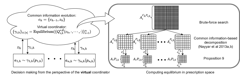
Figure 1: An overview of our algorithmic framework. The left part of the figure shows that there is a virtual coordinator collecting the information shared among agents. Based on the common information $c_{h}$, it will compute an equilibrium in the prescription space and assign it to all the agents. The right part shows the computation of equilibrium. Let’s take the example of $A_{i}=2$, $P_{i,h}=3$, $C_{h}=2$. If we search over all deterministic prescriptions, the corresponding matrix game will have the size of $A_{i}^{C_{h}P_{i,h}}=64$. Then, Nayyar et al. (2013a, b) propose the common information-based decomposition, and solve $C_{h}$ number of games of smaller size. However, in the Dec-POMDP setting, Nayyar et al. (2013b) treats each deterministic prescription as an action and the size of each sub-problem will be $A_{i}^{P_{i,h}}=8$. Furthermore, Proposition 9 shows that we can reformulate each sub-problem as a game whose payoff is multi-linear with respect to each agent’s prescription, and whose dimensionality is $A_{i}P_{i,h}=6$.

Criteria of information-sharing design for efficient planning.

Now we sketch the criteria for designing the information-sharing strategy for efficient planning using our algorithms before:

• The POSG $\mathcal{G}$ satisfies Assumptions 1 and 3.

• Cardinality of $\{\mathcal{P}_{h}\}_{h\in[H+1]}$ should be small.

• Cardinality of $\{\widehat{\mathcal{C}}_{h}\}_{h\in[H+1]}$ should be small.

• Construction of the expected approximate common information model $\mathcal{M}$, i.e., the construction of $\mathbb{E}^{\mathcal{M}}[\widehat{r}_{i,h+1}(o_{h+1}){\,|\,}\widehat{c}_{h},{\gamma}_{h}]$ and $\mathbb{P}_{h}^{\mathcal{M},z}(\cdot{\,|\,}\widehat{c}_{h},{\gamma}_{h})$ should be computationally efficient.

Planning in observable POSGs without intractable oracles.

Theorem 2 applies to any expected approximate common information model as given in Definition 8, by substituting the corresponding $\widehat{C}_{h}$. Note that it does not provide a way to construct such expected approximate common information models that ensure the computation complexity in the theorem is quasi-polynomial.

Next, we show that in several natural and standard information structure examples, a simple finite-memory compression can attain the goal of computing $\epsilon$-NE/CE/CCE without intractable oracles, where we refer to §D.4 for the concrete form of the finite-memory compression. Based on this, we present the corresponding quasi-polynomial time complexities as follows.

Theorem 3.

Fix $\epsilon>0$. Suppose there exists an $(\epsilon_{r},\epsilon_{z})$-expected-approximate common information model $\mathcal{M}$ consistent with some given approximate belief $\{\mathbb{P}_{h}^{\mathcal{M},c}(s_{h},p_{h}{\,|\,}\widehat{c}_{h})\}_{h\in[H]}$ for the POSG $\mathcal{G}$ that satisfies Assumptions 1 and 3, with $\max\{\epsilon_{z},\epsilon_{r}\}\leq\mathcal{O}(\epsilon)$. Moreover, suppose $\max_{h}\widehat{C}_{h}P_{h}$ is quasi-polynomial of the problem instance size. Then, there exists a quasi-polynomial time algorithm that can compute an $\epsilon$-NE if $\mathcal{G}$ is zero-sum or cooperative, and an $\epsilon$-CE/CCE if $\mathcal{G}$ is general-sum.

In particular, under Assumption 2, all the examples in §3 satisfy the conditions above. Therefore, there exists a quasi-polynomial time algorithm that can compute an $\epsilon$-NE if $\mathcal{G}$ is zero-sum or cooperative, and an $\epsilon$-CE/CCE if $\mathcal{G}$ is general-sum, with the information-sharing structures in §3.

5.2 Statistically (quasi-)efficient learning

Until now, we have been assuming the full knowledge of the model $\mathcal{G}$ (the transition kernel, observation emission, and reward functions). In this full-information setting, we are able to construct some model $\mathcal{M}$ to approximate the true $\mathcal{G}$ according to the conditions we identified in Definition 8. However, when we only have access to the samples drawn from the POSG $\mathcal{G}$, it is difficult to directly construct such a model $\mathcal{M}$ due to the lack of the model specification. To address this issue, the solution is to construct a specific expected approximate common information model that depends on the policies that generate the data for such a construction, which can be denoted by $\tilde{\mathcal{M}}(\pi^{1:H})$. For such a model, one could simulate and sample by running policies $\pi^{1:H}$ in the true model $\mathcal{G}$. To introduce such a model $\tilde{\mathcal{M}}(\pi^{1:H})$, we have the following formal definition.

Definition 10 (Policy-dependent approximate common information model).

Given an expected approximate common information model $\tilde{\mathcal{M}}$ (as in Definition 8), and given $H$ joint policies $\pi^{1:H}$, where $\pi^{h}\in\Delta({}^{\mathrm{gen}})$ for $h\in[H]$, we say $\tilde{\mathcal{M}}$ is a policy-dependent expected approximate common information model, denoted as $\tilde{\mathcal{M}}(\pi^{1:H})$, if it is consistent with the policy-dependent belief $\{\mathbb{P}_{h}^{\pi^{h},\mathcal{G}}(s_{h},p_{h}{\,|\,}\widehat{c}_{h})\}_{h\in[H]}$ as per Definition 9, where $\mathbb{P}_{h}^{\pi^{h},\mathcal{G}}(s_{h},p_{h}{\,|\,}\widehat{c}_{h})$ can be computed by running policy $\pi^{h}$ in the true model $\mathcal{G}$, and using $\text{Compress}_{h}$ together with Bayes rule.

The key to the definition above resorts to an approximate common information-based conditional belief $\{\mathbb{P}_{h}^{\pi^{h},\mathcal{G}}(s_{h},p_{h}{\,|\,}\widehat{c}_{h})\}_{h\in[H]}$ that is defined by running policy $\pi^{h}\in\Delta({}^{\mathrm{gen}})$ in $\mathcal{G}$. In particular, we have the following fact directly from Definition 9.

Proposition 4.

Given $\tilde{\mathcal{M}}(\pi^{1:H})$ as in Definition 10, it holds that for any $h\in[H]$, $\widehat{c}_{h}\in\widehat{\mathcal{C}}_{h}$, $\gamma_{h}\in{}_{h}$, $o_{h+1}\in\mathcal{O}$, $z_{h+1}\in\mathcal{Z}_{h+1}$:

$$\mathbb{P}_{h}^{\tilde{\mathcal{M}}(\pi^{1:H}),z}(z_{h+1}{\,|\,}\widehat{c}_{h},{\gamma}_{h})=\mathbb{P}_{h}^{\pi^{h}_{1:h-1},\mathcal{G}}(z_{h+1}{\,|\,}\widehat{c}_{h},{\gamma}_{h}),\qquad\qquad\mathbb{P}_{h}^{\tilde{\mathcal{M}}(\pi^{1:H}),o}(o_{h+1}{\,|\,}\widehat{c}_{h},{\gamma}_{h})=\mathbb{P}_{h}^{\pi^{h}_{1:h-1},\mathcal{G}}(o_{h+1}{\,|\,}\widehat{c}_{h},{\gamma}_{h}).$$

This proposition verifies that we can have access to the samples from the transition and reward of $\tilde{\mathcal{M}}(\pi^{1:H})$ at step $h$, by executing policy $\pi^{h}$ in the underlying model $\mathcal{G}$. Now we present the main theorem for learning such an expected approximate common information model $\tilde{\mathcal{M}}(\pi^{1:H})$. A major difference from the analysis for planning is that in the learning setting, we need to explore the space of approximate common information, which is a function of a sequence of observations and actions, and we need to characterize the length of the approximate common information as defined below.

Definition 11 (Length of approximate common information).

Given $\{\widehat{\mathcal{C}}_{h}\}_{h\in[H+1]}$, define the integer $\widehat{L}\geq 0$ as the minimum length such that for each $h\in[H+1]$ and each $\widehat{c}_{h}\in\widehat{\mathcal{C}}_{h}$, there exists some mapping $\widehat{f}_{h}:\mathcal{A}^{\min\{\widehat{L},h\}}\times\mathcal{O}^{\min\{\widehat{L},h\}}\rightarrow\widehat{\mathcal{C}}_{h}$ and the sequence $x_{h}=\{a_{\max\{h-\widehat{L},1\}},o_{\max\{h-\widehat{L},1\}+1},\cdots,o_{h}\}$, such that $\widehat{f}_{h}(x_{h})=\widehat{c}_{h}$.

Such an $\widehat{L}$ characterizes the length of the constructed approximate common information, for which our final sample complexity would necessarily depend on, since we need to do exploration for the steps after $h-\widehat{L}$, and $\widehat{L}$ characterizes the cardinality of the space to be explored. It is worth noting that such an $\widehat{L}$ always exists since we can always set $\widehat{L}=H$, and there always exists the mapping $\widehat{f}_{h}$ such that $\widehat{f}_{h}(a_{1:h-1},o_{2:h})=\widehat{c}_{h}$, where $\widehat{f}_{h}$ is a composition of the mapping from $\{a_{1:h-1},o_{2:h}\}$ to $c_{h}$, which is given by the evolution rules in Definition 1, and the compression function $\operatorname{Compress}_{h}$, the mapping from $c_{h}$ to $\widehat{c}_{h}$. With this definition of $\widehat{L}$, we propose Algorithm 5, which learns the model $\tilde{\mathcal{M}}(\pi^{1:H})$, mainly the two quantities $\mathbb{P}_{h}^{\tilde{\mathcal{M}}(\pi^{1:H}),z}$ and $\mathbb{P}_{h}^{\tilde{\mathcal{M}}(\pi^{1:H}),o}$ in Proposition 4, by executing policies $\pi^{1:H}$ in the true model $\mathcal{G}$, with the following sample complexity depending on $\widehat{L}$.

Theorem 4.

Suppose the POSG $\mathcal{G}$ satisfies Assumptions 1 and 3. Given any compression functions of common information, $\operatorname{Compress}_{h}:\mathcal{C}_{h}\rightarrow\widehat{\mathcal{C}}_{h}$ for $h\in[H+1]$, we can compute $\widehat{L}$ as defined in Definition 11. Then, given any $H$ policies $\pi^{1:H}$, where $\pi^{h}\in\Delta({}^{\mathrm{gen}})$, $\pi^{h}_{h-\widehat{L}:h}=\operatorname{Unif}(\mathcal{A})$ for $h\in[H]$, we can construct a policy-dependent expected approximate common information model $\tilde{\mathcal{M}}(\pi^{1:H})$, whose compression functions are $\{\operatorname{Compress}_{h}\}_{h\in[H+1]}$. We write $\epsilon_{r}(\pi^{1:H},\widehat{r}):=\epsilon_{r}(\tilde{\mathcal{M}}(\pi^{1:H}))$ and $\epsilon_{z}(\pi^{1:H}):=\epsilon_{z}(\tilde{\mathcal{M}}(\pi^{1:H}))$ for short. Note that according to the definition of $\tilde{\mathcal{M}}(\pi^{1:H})$, $\epsilon_{r}$ depends on $\pi^{1:H}$ and $\widehat{r}$, while $\epsilon_{z}$ depends on $\pi^{1:H}$ only. Fix the parameters $\delta_{1},\theta_{1},\theta_{2},\zeta_{1},\zeta_{2}>0$ for Algorithm 5, $\epsilon_{e}>0$ for Algorithm 3, and some $\phi>0$, define the approximation error for estimating $\tilde{\mathcal{M}}(\pi^{1:H})$ using samples under the policies $\pi^{1:H}$ as $\epsilon_{apx}(\pi^{1:H},\widehat{L},\zeta_{1},\zeta_{2},\theta_{1},\theta_{2},\phi)$ (see definition in Equation (C.1)). Then Algorithm 5, together with Algorithm 3, can output an $\epsilon$-NE if $\mathcal{G}$ is zero-sum or cooperative, and an $\epsilon$-CE/CCE if $\mathcal{G}$ is general-sum, with probability at least $1-\delta_{1}$, with sample complexity $N_{0}=\operatorname{poly}(\max_{h\in[H]}P_{h},\max_{h\in[H]}\widehat{C}_{h},H,A,O,\frac{1}{\zeta_{1}},\frac{1}{\zeta_{2}},\frac{1}{\theta_{1}},\frac{1}{\theta_{2}})\cdot\log\frac{1}{\delta_{1}}$, where $\epsilon:=H\epsilon_{r}(\pi^{1:H},\widehat{r})+H^{2}\epsilon_{z}(\pi^{1:H})+(H^{2}+H)\epsilon_{apx}(\pi^{1:H},\widehat{L},\zeta_{1},\zeta_{2},\theta_{1},\theta_{2},\phi)+H\epsilon_{e}.$

A detailed version of this theorem is deferred to §C.2. This meta-theorem builds on a sample complexity guarantee of learning expected approximate common information model $\tilde{\mathcal{M}}(\pi^{1:H})$ under the approximate common-information framework, in the model-free setting. The result holds for any choices of compression functions, policies $\pi^{1:H}$, and approximate reward function $\widehat{r}$. Therefore, the final results will necessarily depend on the three error terms $\epsilon_{r}(\pi^{1:H},\widehat{r})$, $\epsilon_{z}(\pi^{1:H})$, and $\epsilon_{apx}(\pi^{1:H},\widehat{L},\zeta_{1},\zeta_{2},\theta_{1},\theta_{2},\phi)$ (see Equation (C.1)), which will be instantiated for different examples later to obtain both sample and time complexity results. As before, the meta-theorem applies to cases beyond the following examples, as long as one can compress the common information properly. The examples below just happen to be the ones where a simple finite-memory truncation can give us desired complexities.

Sample (quasi-)efficient learning in POSGs without intractable oracles.

Now we apply the meta-theorem, Theorem 4, and obtain quasi-polynomial time and sample complexities for learning the $\epsilon$-NE/CE/CCE, under several standard information structures.

Theorem 5.

Fix $\epsilon,\delta>0$. Suppose the POSG $\mathcal{G}$ satisfies Assumptions 1 and 3. If there exist some compression functions of common information, $\operatorname{Compress}_{h}:\mathcal{C}_{h}\rightarrow\widehat{\mathcal{C}}_{h}$ for $h\in[H+1]$, $\pi^{1:H}$, and $\tilde{\mathcal{M}}(\pi^{1:H})$ satisfying the conditions in Theorem 4, and there exist some parameters $\delta_{1},\theta_{1},\theta_{2},\zeta_{1},\zeta_{2}>0$ for Algorithm 5, $\epsilon_{e}>0$ for Algorithm 3, and some $\phi>0$, such that

$$\max\left\{\epsilon_{z}(\pi^{1:H}),\epsilon_{r}(\pi^{1:H},\widehat{r}),\epsilon_{apx}(\pi^{1:H},\widehat{L},\zeta_{1},\zeta_{2},\theta_{1},\theta_{2},\phi)\right\}\leq\mathcal{O}(\epsilon)$$

and $N_{0}=\operatorname{poly}(\max_{h\in[H]}P_{h},\max_{h}\widehat{C}_{h\in[H]},H,A,O,\frac{1}{\zeta_{1}},\frac{1}{\zeta_{2}},\frac{1}{\theta_{1}},\frac{1}{\theta_{2}})\cdot\log\frac{1}{\delta_{1}}$ is quasi-polynomial of the problem instance size, then Algorithm 5 together with Algorithm 3 can output an $\epsilon$-NE if $\mathcal{G}$ is zero-sum or cooperative, and an $\epsilon$-CE/CCE if $\mathcal{G}$ is general-sum, with probability at least $1-\delta$, using quasi-polynomial time and samples, where $\widehat{L}$ is defined as in Definition 11.

In particular, under Assumption 2, all the examples in §3 satisfy the conditions above. Therefore, for all the information-sharing structures in §3, there exists a multi-agent RL algorithm that learns an $\epsilon$-NE if $\mathcal{G}$ is zero-sum or cooperative, and an $\epsilon$-CE/CCE if $\mathcal{G}$ is general-sum, with probability at least $1-\delta$, in time and sample complexities that are both quasi-polynomial.

A full version of the theorem is presented in §C.2, with proof provided in §D.5. Note that our algorithm is computationally (quasi-)efficient, in contrast to the only existing sample-efficient MARL algorithm for POSGs in Liu et al. (2022b), which relies on computationally intractable oracles.

Algorithm description.

We briefly introduce the algorithm that achieves the guarantees in Theorem 5, i.e., Algorithm 7, and defer more details to §B due to space limitation. The first step is to find the approximate reward function $\widehat{r}$ and policies $\pi^{1:H}$ such that the three error terms $\epsilon_{apx}(\pi^{1:H},\widehat{L},\zeta_{1},\zeta_{2},\theta_{1},\theta_{2},\phi)$, $\epsilon_{r}(\pi^{1:H},\widehat{r})$, and $\epsilon_{z}(\pi^{1:H})$ in Theorem 4 are minimized. It turns out that the three errors can be minimized using Barycentric-Spanner-based (Awerbuch and Kleinberg, 2008; Golowich et al., 2022a) exploration techniques. The next step is to learn the empirical estimate $\widehat{\mathcal{M}}(\pi^{1:H})$ of $\tilde{\mathcal{M}}(\pi^{1:H})$, by exploring the approximate common information space $\{\widehat{\mathcal{C}}_{h}\}_{h\in[H+1]}$ using Algorithm 5. The key to exploring the approximate common information space is to take uniformly random actions from steps $h-\widehat{L}$ to $h$, which has been used for exploration in finite-memory based state spaces in existing works (Efroni et al., 2022; Golowich et al., 2022a). Once such a $\widehat{\mathcal{M}}(\pi^{1:H})$ is constructed, we run our planning algorithms (developed in §5.1) on $\widehat{\mathcal{M}}(\pi^{1:H})$ to compute an approximate NE/CE/CCE. The final step is to do policy evaluation to select the equilibrium policy to output, since for the first step we may only obtain a set of $\{\pi^{1:H,j},\widehat{r}^{j}\}_{j\in[K]}$ for some integer $K>0$ and only some of them can minimize the three error terms. Specifically, for any given policy $\pi^{\star}$ and $i\in[n]$, the key idea of policy evaluation is that we compute its best response introduced in Algorithm 4 in all the models $\{\widehat{\mathcal{M}}(\pi^{1:H,j})\}_{j\in[K]}$, where $K=\operatorname{poly}(H,S)$ to get $\{\pi_{-i}^{\star,j}\}_{j\in[K]}$ and select the one $\pi_{-i}^{\star,\widehat{j}}$ for some $\widehat{j}$ with the highest empirical rewards by rolling them out in the true model $\mathcal{G}$. With the guarantee that there must be a $j\in[K]$ such that $\widehat{\mathcal{M}}(\pi^{1:H,j})$ is a good approximation of $\mathcal{G}$ in the sense of Definition 8, it can be shown that $\pi_{-i}^{\star,\widehat{j}}$ will be an approximate best response in $\mathcal{G}$ with high probability. With the best-response policy, we can select the equilibrium policy with the lowest NE/CE/CCE-gap, which turns out to be an approximate NE/CE/CCE in $\mathcal{G}$ with high probability.

6 Experimental Results

Figure 2: Performance of MAPPO and IPPO in various delayed-sharing settings.

For the experiments, we shall both investigate the benefits of information sharing as we considered in various empirical MARL environments, and validate the implementability and performance of our proposed approaches on several modest-scale examples.

Information sharing improves performance.

We consider the popular deep MARL benchmarks, multi-agent particle-world environment (MPE) (Lowe et al., 2017). We mainly consider three cooperative tasks, the physical deception task (Spread), the simple reference task (Reference), and the cooperative communication task (Comm). In those tasks, the agent needs to learn to take physical actions in the environment and communication actions that get broadcasted to other agents. We train both the popular centralized-training algorithm MAPPO (Yu et al., 2021) and the decentralized-training algorithm IPPO (Yu et al., 2021) with different information-sharing mechanisms by varying the information-sharing delay from $0$ to $\infty$. For the centralized MAPPO, we also adopt parameter sharing when agents are homogenous, which is reported as important for improved performance. For decentralized IPPO, we do not enforce any coordination during training among agents. Note that the original algorithm in Yu et al. (2021) corresponds to the case, where the delay is $d=\infty$. The rewards during training are shown in Figure 2. It is seen that in all domains (except MAPPO on Spread) with either centralized training or decentralized training, smaller delays, which correspond to the case of more information sharing, will lead to faster convergence, higher final performance, and reduced training variance. For decentralized training where coordination is absent, sharing information could be more useful.

	Boxpushing				Dectiger
Horizon	Ours	FM-E	RNN-E		Ours	FM-E	RNN-E
3	62.78	64.22	8.40		13.06	-6.0	-6.0
4	81.44	77.80	9.10		20.89	-4.76	-7.00
5	98.73	96.40	21.78		27.95	-6.37	-10.04
6	98.76	94.61	94.36		36.03	-7.99	-11.90
7	145.35	138.44	132.70		37.72	-7.99	-13.92

Table 1: Final evaluation of the rewards using our methods, compared with using the methods of FM-E and RNN-E in Mao et al. (2020).

Validating implementability and performance.

To further validate the tractability of our approaches, we test our learning algorithm on two popular and modest-scale partially observable benchmarks Dectiger (Nair et al., 2003) and Boxpushing (Seuken and Zilberstein, 2012). Furthermore, to be compatible with popular deep RL algorithms, we fit the transition using neural networks instead of the counting methods adopted in Algorithm 7. For the planning oracles used in Algorithm 7, we choose to use Q-learning instead of backward-induction style algorithms as in Algorithm 3, for which we found working well empirically. Finally, for finite memory compression, we used a finite window of length of $4$. Both our algorithm and baselines are trained with $80000$ time steps. We compare our approaches with two baselines, FM-E and RNN-E, which are also common information-based approaches in Mao et al. (2020). The final rewards are reported in Table 1. In both domains with various horizons, our methods consistently outperform the baselines.

7 Concluding Remarks

In this paper, we studied provable multi-agent RL in partially observable environments, with both statistical and computational (quasi-)efficiencies. The key to our results is to identify the value of information sharing, a common practice in empirical MARL and a standard phenomenon in many multi-agent control system applications, in algorithm design and computation/sample efficiency analysis. We hope our study may open up the possibilities of leveraging and even designing different information structures, for developing both statistically and computationally efficient partially observable MARL algorithms. One open problem and future direction is to develop a fully decentralized algorithm and overcome the curse of multiagents, such that the sample and computation complexities do not grow exponentially with the number of agents. Another interesting direction is to identify the combination of certain information-sharing structures and observability assumptions that allows more efficient (e.g., polynomial) sample and computation complexity results.

Appendices

Appendix A Additional Definitions

A.1 Belief states

In such partially observable games, each agent cannot know the underlying state but could infer the underlying distribution of states through the observations and actions. Following the convention in POMDPs, we call such distributions the belief states. Such posterior distributions over states can be updated whenever the agent receives new observations and actions. Formally, we define the belief update as:

Definition 12 (Belief state update).

For each $h\in[H+1]$, the Bayes operator (with respect to the joint observation) $B_{h}:\Delta({\mathcal{S}})\times\mathcal{O}\rightarrow\Delta({\mathcal{S}})$ is defined for $b\in\Delta({\mathcal{S}})$, and $y\in\mathcal{O}$ by:

$$B_{h}(b;y)(x)=\frac{\mathbb{O}_{h}(y\mid x)b(x)}{\sumop\displaylimits_{z\in\mathcal{S}}\mathbb{O}_{h}(y\mid z)b(z)}.$$

Similarly, for each $h\in[H],i\in[n]$, we define the Bayes operator with respect to individual observations $B_{i,h}:\Delta({\mathcal{S}})\times\mathcal{O}_{i}\rightarrow\Delta({\mathcal{S}})$ by:

$$B_{i,h}(b;y)(x)=\frac{\mathbb{O}_{i,h}(y\mid x)b(x)}{\sumop\displaylimits_{z\in\mathcal{S}}\mathbb{O}_{i,h}(y\mid z)b(z)}.$$

For each $h\in[H]$, the belief update operator $U_{h}:\Delta(\mathcal{S})\times\mathcal{A}\times\mathcal{O}\rightarrow\Delta(\mathcal{S})$, is defined by

$$U_{h}(b;a,y)=B_{h+1}\left(\mathbb{T}_{h}(a)\cdot b;y\right),$$

where $\mathbb{T}_{h}(a)\cdot b$ represents the matrix multiplication. We use the notation $\bm{b}_{h}$ to denote the belief update function, which receives a sequence of actions and observations and outputs a distribution over states at the step $h$: the belief state at step $h=1$ is defined as $\bm{b}_{1}(\emptyset)=\mu_{1}$. For any $2\leq h\leq H$ and any action-observation sequence $(a_{1:h-1},o_{2:h})$, we inductively define the belief state:

$$\bm{b}_{h+1}(a_{1:h},o_{2:h}) =\mathbb{T}_{h}(a_{h})\cdot\bm{b}_{h}(a_{1:h-1},o_{2:h}),$$

$$\bm{b}_{h}(a_{1:h-1},o_{2:h}) =B_{h}(\bm{b}_{h}(a_{1:h-1},o_{2:h-1});o_{h}).$$

Also, we slightly abuse the notation and define the belief state containing individual observations as

$$\bm{b}_{h}(a_{1:h-1},o_{2:h-1},o_{i,h})=B_{i,h}(\bm{b}_{h}(a_{1:h-1},o_{2:h-1});o_{i,h}).$$

We also define the approximate belief update using the most recent $L$-step history. For $1\leq h\leq H$, we follow the notation of Golowich et al. (2022b) and define

$$\bm{b}_{h}^{\mathrm{apx},\mathcal{G}}(\emptyset;{D})=\begin{cases}\mu_{1}&\text{ if }h=1\\ {D}&\text{ otherwise },\end{cases}$$

where ${D}\in\Delta({\mathcal{S}})$ is the prior for the approximate belief update. Then for any $1\leq h-L<h\leq H$ and any action-observation sequence $(a_{h-L:h-1},o_{h-L+1:h})$, we inductively define

$$\bm{b}_{h+1}^{\mathrm{apx},\mathcal{G}}(a_{h-L:h},o_{h-L+1:h};{D}) =\mathbb{T}_{h}(a_{h})\cdot\bm{b}^{\mathrm{apx},\mathcal{G}}_{h}(a_{h-L:h-1},o_{h-L+1:h};{D}),$$

$$\bm{b}_{h}^{\mathrm{apx},\mathcal{G}}(a_{h-L:h-1},o_{h-L+1:h};{D}) =B_{h}(\bm{b}^{\mathrm{apx},\mathcal{G}}_{h}(a_{h-L:h-1},o_{h-L+1:h-1};{D});o_{h}).$$

For the remainder of our paper, we shall use the important initialization for the approximate belief, which are defined as $\bm{b}^{\prime}_{h}(\cdot):=\bm{b}_{h}^{\mathrm{apx},\mathcal{G}}(\cdot;\operatorname{Unif}({\mathcal{S}}))$.

A.2 Additional definitions of value functions and policies

With the expected approximate common information model $\mathcal{M}$ given in Definition 8, we can define the value function and policy under $\mathcal{M}$ accordingly as follows.

Definition 13 (Value function and policy under $\mathcal{M}$).

Given an expected approximate common information model $\mathcal{M}$. For any policy $\pi\in\Pi$, for each $i\in[n],h\in[H]$, we define the value function as

$$V^{{\pi},\mathcal{M}}_{i,h}(c_{h})=\mathbb{E}_{\{\omega_{j,h}\}_{j\in[n]}}\mathbb{E}^{\mathcal{M}}[\widehat{r}_{i,h+1}(o_{h+1})+V^{{\pi},\mathcal{M}}_{i,h+1}(c_{h+1}){\,|\,}\widehat{c}_{h},{\{\pi_{j,h}(\cdot{\,|\,}\omega_{j,h},c_{h},\cdot)_{j\in[n]}\}}].$$ (A.1)

For any $c_{H+1}\in\mathcal{C}_{H+1}$, we define $V_{i,H+1}^{\pi,\mathcal{M}}(c_{H+1})=0$. Furthermore, for a policy $\widehat{\pi}$ whose $\widehat{\pi}_{i,h}:{}_{h}\times\mathcal{P}_{i,h}\times\widehat{\mathcal{C}}_{h}\rightarrow\Delta({\mathcal{A}_{i}})$ takes approximate instead of the exact common information as the input, we define

$$V^{{\widehat{\pi}},\mathcal{M}}_{i,h}(\widehat{c}_{h})=\mathbb{E}_{\{\omega_{j,h}\}_{j\in[n]}}\mathbb{E}^{\mathcal{M}}[\widehat{r}_{i,h+1}(o_{h+1})+V^{\widehat{\pi},\mathcal{M}}_{i,h+1}(\widehat{c}_{h+1}){\,|\,}\widehat{c}_{h},\{\widehat{\pi}_{j,h}(\cdot{\,|\,}\omega_{j,h},\widehat{c}_{h},\cdot)_{j\in[n]}\}],$$ (A.2)

where similarly, for each $\widehat{c}_{H+1}\in\widehat{\mathcal{C}}_{H+1}$, we define $V^{\widehat{\pi},\mathcal{M}}_{i,H+1}(\widehat{c}_{H+1})=0$. With a slight abuse of notation, sometimes $\widehat{\pi}_{i,h}$ may also take $c_{h}\in\mathcal{C}_{h}$ as input and thus $\widehat{\pi}\in\Pi$. In this case, when $\mathcal{M}$ and the corresponding compression function $\operatorname{Compress}_{h}$ are clear from the context, it means $\widehat{\pi}_{i,h}(\cdot{\,|\,}\cdot,c_{h},\cdot):=\widehat{\pi}_{i,h}(\cdot{\,|\,}\cdot,\operatorname{Compress}_{h}(c_{h}),\cdot)$. Accordingly, in this case, the definitions of $V_{i,h}^{\widehat{\pi},\mathcal{G}}(c_{h})$ and $V_{i,h}^{\widehat{\pi},\mathcal{M}}(c_{h})$ follows from Definition 1 and Equation (A.1), respectively.

Appendix B Collection of Algorithm Pseudocodes

Here we collect both our planning and learning algorithms as in Algorithms 1, 2, 3, 4, 5, 6.

Algorithm 1 Value iteration with common information

Input: $\mathcal{G},\epsilon_{e}$

for each $i\in[n]$ and $c_{H+1}$ do

     $V^{\star,\mathcal{G}}_{i,H+1}(c_{H+1})\leftarrow 0$

end for

for $h=H,\cdots,1$ do

     for each $c_{h}$ do

         Define $Q^{\star,\mathcal{G}}_{i,h}(c_{h},\gamma_{1,h},\cdots,\gamma_{n,h}):=\mathbb{E}_{s_{h},p_{h}\sim\mathbb{P}_{h}^{\mathcal{G}}\left(\cdot,\cdot{\,|\,}c_{h}\right)}\mathbb{E}_{\{a_{j,h}\sim{\gamma}_{j,h}(\cdot{\,|\,}p_{j,h})\}_{j\in[n]}}\mathbb{E}_{o_{h+1}\sim\mathbb{O}_{h+1}^{\top}\mathbb{T}_{h}(\cdot{\,|\,}s_{h},a_{h})}[r_{i,h+1}(o_{h+1})+V^{\star,\mathcal{G}}_{i,h+1}(c_{h+1})]$

         $\big{(}\pi_{1,h}^{\star}(\cdot{\,|\,}\cdot,c_{h},\cdot),\cdots,\pi_{n,h}^{\star}(\cdot{\,|\,}\cdot,c_{h},\cdot)\big{)}\leftarrow\operatorname{NE/CE/CCE}(\{Q_{i,h}^{\star,\mathcal{G}}(c_{h},\cdot,\cdots,\cdot)\}_{i=1}^{n},\epsilon_{e})$ // we refer the implementation to §D.2

         for each $i\in[n]$ do

$$V^{\star,\mathcal{G}}_{i,h}(c_{h})\leftarrow\mathbb{E}_{\{\omega_{j,h}\}_{j\in[n]}}\mathbb{E}_{s_{h},p_{h}\sim\mathbb{P}_{h}^{\mathcal{G}}\left(\cdot,\cdot{\,|\,}c_{h}\right)}\mathbb{E}_{\{a_{j,h}\sim\pi^{\star}_{j,h}(\cdot{\,|\,}\omega_{j,h},c_{h},p_{j,h})\}_{j\in[n]}}\mathbb{E}_{o_{h+1}\sim\mathbb{O}_{h+1}^{\top}\mathbb{T}_{h}(\cdot{\,|\,}s_{h},a_{h})}[r_{i,h+1}(o_{h+1})+V^{\star,\mathcal{G}}_{i,h+1}(c_{h+1})]$$

         end for

     end for

end for

return $\pi^{\star}$

Algorithm 2 BR$(\mathcal{G},\pi,i,\epsilon_{e})$: $\epsilon_{e}$-approximate Best Response for agent $i$ under true model $\mathcal{G}$

Input: $\mathcal{G},\pi,i,\epsilon_{e}$

${V}^{\star,\mathcal{G}}_{i,H+1}({c}_{H+1})\leftarrow 0$ for all ${c}_{H+1}$

for $h=H,\cdots,1$ do

     for each ${c}_{h}$ do

         Define ${Q}^{\star,\mathcal{G}}_{i,h}({c}_{h},\gamma_{1,h},\cdots,\gamma_{n,h}):=\mathbb{E}_{s_{h},p_{h}\sim\mathbb{P}_{h}^{\mathcal{G}}\left(\cdot,\cdot{\,|\,}c_{h}\right)}\mathbb{E}_{\{a_{j,h}\sim{\gamma}_{j,h}(\cdot{\,|\,}p_{j,h})\}_{j\in[n]}}\mathbb{E}_{o_{h+1}\sim\mathbb{O}_{h+1}^{\top}\mathbb{T}_{h}(\cdot{\,|\,}s_{h},a_{h})}[r_{i,h+1}(o_{h+1})+V^{\star,\mathcal{G}}_{i,h+1}(c_{h+1})]$

         ${\pi}_{i,h}^{\star}(\cdot{\,|\,}\cdot,{c}_{h},\cdot)\leftarrow\operatorname{NE/CE/CCE-BR}({Q}_{i,h}^{\star,\mathcal{G}}({c}_{h},\cdot,\cdots,\cdot),\{\pi_{j,h}(\cdot{\,|\,}\cdot,{c}_{h},\cdot)\}_{j\in[n]},i,\epsilon_{e})$  // we refer the implementation to §D.2

         ${V}^{\star,\mathcal{G}}_{i,h}({c}_{h})\leftarrow\mathbb{E}_{\{\omega_{j,h}\}_{j\in[n]}}\mathbb{E}_{s_{h},p_{h}\sim\mathbb{P}_{h}^{\mathcal{G}}\left(\cdot,\cdot{\,|\,}c_{h}\right)}\mathbb{E}_{a_{i,h}\sim\pi_{i,h}^{\star}(\cdot{\,|\,}\omega_{i,h},c_{h},p_{i,h}),a_{-i,h}\sim\pi_{-i,h}(\cdot{\,|\,}\omega_{-i,h},c_{h},p_{-i,h})}\mathbb{E}_{o_{h+1}\sim\mathbb{O}_{h+1}^{\top}\mathbb{T}_{h}(\cdot{\,|\,}s_{h},a_{h})}[r_{i,h+1}(o_{h+1})+V^{\star,\mathcal{G}}_{i,h+1}(c_{h+1})]$

     end for

end for

return ${\pi}_{i}^{\star}$

Algorithm 3 VIACM$(\mathcal{M},\epsilon_{e})$: Value Iteration with expected Approximate Common-information Model

Input: $\mathcal{M},\epsilon_{e}$

for each $i\in[n]$ and $\widehat{c}_{H+1}$ do

     ${V}^{\star,\mathcal{M}}_{i,H+1}(\widehat{c}_{H+1})\leftarrow 0$

end for

for $h=H,\cdots,1$ do

     for each $\widehat{c}_{h}$ do

         Define ${Q}^{\star,\mathcal{M}}_{i,h}(\widehat{c}_{h},\gamma_{1,h},\cdots,\gamma_{n,h})\vcentcolon=\mathbb{E}^{\mathcal{M}}[\widehat{r}_{i,h+1}(o_{h+1})+{V}^{\star,\mathcal{M}}_{i,h+1}(\widehat{c}_{h+1})\mid\widehat{c}_{h},\{\gamma_{j,h}\}_{j\in[n]}]$ for any $i\in[n]$

         $\big{(}\widehat{\pi}_{1,h}^{\star}(\cdot{\,|\,}\cdot,\widehat{c}_{h},\cdot),\cdots,\widehat{\pi}_{n,h}^{\star}(\cdot{\,|\,}\cdot,\widehat{c}_{h},\cdot)\big{)}\leftarrow\operatorname{NE/CE/CCE}(\{{Q}_{i,h}^{\star,\mathcal{M}}(\widehat{c}_{h},\cdot,\cdots,\cdot)\}_{i=1}^{n},\epsilon_{e})$ // we refer the implementation to §D.2

         for each $i\in[n]$ do

              ${V}^{\star,\mathcal{M}}_{i,h}(\widehat{c}_{h})\leftarrow\mathbb{E}_{\{\omega_{j,h}\}_{j\in[n]}}\mathbb{E}^{\mathcal{M}}[\widehat{r}_{i,h+1}(o_{h+1})+{V}^{\star,\mathcal{M}}_{i,h+1}(\widehat{c}_{h+1})\mid\widehat{c}_{h},\{\widehat{\pi}_{j,h}^{\star}(\cdot{\,|\,}\omega_{j,h},\widehat{c}_{h},\cdot)\}_{j\in[n]}]$

         end for

     end for

end for

return $\widehat{\pi}^{\star}$

Algorithm 4 ABR$(\mathcal{M},\widehat{\pi},i,\epsilon_{e})$: $\epsilon_{e}$-approximate Best Response for agent $i$ under Approximate common information model $\mathcal{M}$

Input: $\mathcal{M},\widehat{\pi},i,\epsilon_{e}$

${V}^{\star,\mathcal{M}}_{i,H+1}(\widehat{c}_{H+1})\leftarrow 0$ for all $\widehat{c}_{H+1}$

for $h=H,\cdots,1$ do

     for each $\widehat{c}_{h}$ do

         Define ${Q}^{\star,\mathcal{M}}_{i,h}(\widehat{c}_{h},\gamma_{1,h},\cdots,\gamma_{n,h})\vcentcolon=\mathbb{E}^{\mathcal{M}}[\widehat{r}_{i,h+1}(o_{h+1})+{V}^{\star,\mathcal{M}}_{i,h+1}(\widehat{c}_{h+1})\mid\widehat{c}_{h},\{\gamma_{j,h}\}_{j\in[n]}]$

         $\widehat{\pi}_{i,h}^{\star}(\cdot{\,|\,}\cdot,\widehat{c}_{h},\cdot)\leftarrow\operatorname{NE/CE/CCE-BR}({Q}_{i,h}^{\star,\mathcal{M}}(\widehat{c}_{h},\cdot,\cdots,\cdot),\{\widehat{\pi}_{j,h}(\cdot{\,|\,}\cdot,\widehat{c}_{h},\cdot)\}_{j\in[n]},i,\epsilon_{e})$ // we refer the implementation to §D.2

         ${V}^{\star,\mathcal{M}}_{i,h}(\widehat{c}_{h})\leftarrow\mathbb{E}_{\{\omega_{j,h}\}_{j\in[n]}}\mathbb{E}^{\mathcal{M}}[\widehat{r}_{i,h+1}(o_{h+1})+{V}^{\star,\mathcal{M}}_{i,h+1}(\widehat{c}_{h+1})\mid\widehat{c}_{h},\{\widehat{\pi}_{i,h}^{\star}(\cdot{\,|\,}\omega_{i,h},\widehat{c}_{h},\cdot),\widehat{\pi}_{-i,h}(\cdot{\,|\,}\omega_{-i,h},\widehat{c}_{h},\cdot)\}]$

     end for

end for

return $\widehat{\pi}_{i}^{\star}$

Algorithm 5 Construct$(\pi^{1:H},\{\widehat{r}_{i}\}_{i=1}^{n},\{\widehat{\mathcal{C}}_{h}\}_{h\in[H+1]},\{\widehat{\phi}_{h+1}\}_{h\in[H]},\Gamma,\zeta_{1},\zeta_{2},\theta_{1},\theta_{2},\delta_{1})$: Constructing empirical estimator $\widehat{\mathcal{M}}(\pi^{1:H})$ of $\tilde{\mathcal{M}}(\pi^{1:H})$

Input: $\pi^{1:H},\{\widehat{r}_{i}\}_{i=1}^{n},\{\widehat{\mathcal{C}}_{h}\}_{h\in[H+1]},\{\widehat{\phi}_{h+1}\}_{h\in[H]},\Gamma,\zeta_{1},\zeta_{2},\theta_{1},\theta_{2},\delta_{1}$

for $1\leq h\leq H$ do

     Define $N_{0}$ as in Equation (C.2).

     Draw $N_{0}$ independent trajectories by executing the policy $\pi^{h}$, and denote the $k^{th}$ trajectory by $(a_{1:H-1}^{k},o_{2:H}^{k})$, for $k\in[N_{0}]$.

     for each $\widehat{c}_{h}\in\widehat{\mathcal{C}}_{h}$ do

         Define $\varphi(p_{h}):=|\{k:\operatorname{Compress}_{h}(f_{h}(a_{1:h-1}^{k},o_{2:h}^{k}))=\widehat{c}_{h},\text{ and }g_{h}(a_{1:h-1}^{k},o_{2:h}^{k})=p_{h}\}|$.

         Set $\mathbb{P}_{h}^{\widehat{\mathcal{M}}(\pi^{1:H})}(p_{h}{\,|\,}\widehat{c}_{h}):=\frac{\varphi(p_{h})}{\sumop\displaylimits_{p_{h}^{\prime}}\varphi(p_{h}^{\prime})}$ for all $p_{h}\in\mathcal{P}_{h}$.

     end for

     for each $\widehat{c}_{h}\in\widehat{\mathcal{C}}_{h}$, $p_{h}\in\mathcal{P}_{h}$, $a_{h}\in\mathcal{A}$ do

         Define $\psi(o_{h+1}):=|\{k:\operatorname{Compress}_{h}(f_{h}(a_{1:h-1}^{k},o_{2:h}^{k}))=\widehat{c}_{h},g_{h}(a_{1:h-1}^{k},o_{2:h}^{k})=p_{h},a_{h}^{k}=a_{h},\text{ and }o_{h+1}^{k}=o_{h+1}\}|$.

         Set $\mathbb{P}_{h}^{\widehat{\mathcal{M}}(\pi^{1:H})}(o_{h+1}{\,|\,}\widehat{c}_{h},p_{h},a_{h}):=\frac{\psi(o_{h+1})}{\sumop\displaylimits_{o_{h+1}^{\prime}}\psi(o_{h+1}^{\prime})}$ for all $o_{h+1}\in\mathcal{O}$.

     end for

end for

Define for any $h\in[H]$, $\widehat{c}_{h}\in\widehat{\mathcal{C}}_{h}$, $\gamma_{h}\in{}_{h}$, $o_{h+1}\in\mathcal{O}_{h+1}$, $z_{h+1}\in\mathcal{Z}_{h+1}$:

$$\mathbb{P}_{h}^{\widehat{\mathcal{M}}(\pi^{1:H}),z}(z_{h+1}{\,|\,}\widehat{c}_{h},\gamma_{h})\leftarrow\sumop\displaylimits_{p_{h},a_{h},o_{h+1}:\chi_{h+1}(p_{h},a_{h},o_{h+1})=z_{h+1}}\mathbb{P}_{h}^{\widehat{\mathcal{M}}(\pi^{1:H})}(p_{h}{\,|\,}\widehat{c}_{h})\prodop\displaylimits_{i=1}^{n}\gamma_{i,h}(a_{i,h}{\,|\,}p_{i,h})\mathbb{P}_{h}^{\widehat{\mathcal{M}}(\pi^{1:H})}(o_{h+1}{\,|\,}\widehat{c}_{h},p_{h},a_{h})$$

$$\mathbb{P}_{h}^{\widehat{\mathcal{M}}(\pi^{1:H}),o}(o_{h+1}{\,|\,}\widehat{c}_{h},\gamma_{h})\leftarrow\sumop\displaylimits_{p_{h},a_{h}}\mathbb{P}_{h}^{\widehat{\mathcal{M}}(\pi^{1:H})}(p_{h}{\,|\,}\widehat{c}_{h})\prodop\displaylimits_{i=1}^{n}\gamma_{i,h}(a_{i,h}{\,|\,}p_{i,h})\mathbb{P}_{h}^{\widehat{\mathcal{M}}(\pi^{1:H})}(o_{h+1}{\,|\,}\widehat{c}_{h},p_{h},a_{h})$$

return $\widehat{\mathcal{M}}(\pi^{1:H}):=(\{\widehat{\mathcal{C}}_{h}\}_{h\in[H+1]},\{\widehat{\phi}_{h+1}\}_{h\in[H]},\{\mathbb{P}_{h}^{\widehat{\mathcal{M}}(\pi^{1:H}),z},\mathbb{P}_{h}^{\widehat{\mathcal{M}}(\pi^{1:H}),o}\}_{h\in[H]},\Gamma,\{\widehat{r}_{i}\}_{i=1}^{n}$

Algorithm 6 PoS$(\{\widehat{\mathcal{M}}(\pi^{1:H,m})\}_{m\in[K]},\{\pi^{\star,j}\}_{j\in[K]},\epsilon_{e},N_{2})$: Policy Selection

Input: $\{\widehat{\mathcal{M}}(\pi^{1:H,j})\}_{j\in[K]},\{\pi^{\star,j}\}_{j\in[K]},\epsilon_{e},N_{2}$

for $i\in[n],j\in[K],m\in[K]$ do

     $\pi_{i}^{\star,j,m}\leftarrow\texttt{ABR}(\widehat{\mathcal{M}}(\pi^{1:H,m}),\pi^{\star,j},i,\epsilon_{e})$ // i.e., Algorithm 4

end for

for $j\in[K]$ do

     Execute $\pi^{\star,j}$ for $N_{2}$ trajectories and let the mean accumulated reward for player $i$ be $R_{i}^{j}$

end for

for $i\in[n],j\in[K],m\in[K]$ do

     Execute $\pi_{i}^{\star,j,m}\odot\pi_{-i}^{\star,j}$ for $N_{2}$ trajectories and let the mean accumulated reward for player $i$ be $R_{i}^{j,m}$

end for

$\widehat{j}\leftarrow\arg\min_{j\in[K]}\left(\max_{i\in[n]}\max_{m\in[K]}(R_{i}^{j,m}-R_{i}^{j})\right)$

return $\pi^{\star,\widehat{j}}$

Algorithm 7 LACI$(\mathcal{G},\{\widehat{\mathcal{C}}_{h}\}_{h\in[H+1]},\{\widehat{\phi}_{h+1}\}_{h\in[H]},\Gamma,\widehat{L},\epsilon,\delta_{2},\zeta_{1},\zeta_{2},\theta_{1},\theta_{2},\delta_{1},N_{2},\epsilon_{e})$: Learning with Approximate Common Information

Input: $\mathcal{G},\{\widehat{\mathcal{C}}_{h}\}_{h\in[H+1]},\{\widehat{\phi}_{h+1}\}_{h\in[H]},\Gamma,\widehat{L},\epsilon,\delta_{2},\zeta_{1},\zeta_{2},\theta_{1},\theta_{2},\delta_{1},N_{2},\epsilon_{e}$

$\{\pi^{1:H,j}\}_{j=1}^{K},\{\{\widehat{r}_{i}^{j}\}_{i=1}^{n}\}_{j=1}^{K}\leftarrow\texttt{BaSeCAMP}(\mathcal{G},\widehat{L},\epsilon,\delta_{2})$ // i.e., Algorithm 3 of Golowich et al. (2022a)

for $j\in[K]$ do

     $\widehat{\mathcal{M}}(\pi^{1:H,j})\leftarrow\texttt{Construct}(\pi^{1:H,j},\{\widehat{r}_{i}^{j}\}_{i=1}^{n},\{\widehat{\mathcal{C}}_{h}\}_{h\in[H+1]},\{\widehat{\phi}_{h+1}\}_{h\in[H]},\Gamma,\zeta_{1},\zeta_{2},\theta_{1},\theta_{2},\delta_{1})$ // i.e., Algorithm 5

     $\pi^{\star,j}\leftarrow\texttt{VIACM}(\widehat{\mathcal{M}}(\pi^{1:H,j}),\epsilon_{e})$ // i.e., Algorithm 3

end for

$\pi^{\star,\widehat{j}}\leftarrow\texttt{PoS}(\{\widehat{\mathcal{M}}(\pi^{1:H,j})\}_{m=1}^{K},\{\pi^{\star,j}\}_{j=1}^{K},\epsilon_{e},N_{2})$ // i.e., Algorithm 6

return $\pi^{\star,\widehat{j}}$

Appendix C Full Versions of the Results

C.1 Planning

We state and prove our claims regarding planning in POSGs with the fully-sharing structure in §4.1.

Below we state the full version of Theorem 2 regarding the optimality and computational complexity of planning in the expected approximate common information model.

Theorem 6.

Fix $\epsilon_{r},\epsilon_{z},\epsilon_{e}>0$. Suppose there exists an $(\epsilon_{r},\epsilon_{z})$-expected-approximate common information model $\mathcal{M}$ for the POSG $\mathcal{G}$ that satisfies Assumptions 1, 3. Furthermore, if $\mathcal{M}$ is consistent with some given belief $\{\mathbb{P}_{h}^{\mathcal{M},c}(s_{h},p_{h}{\,|\,}\widehat{c}_{h})\}_{h\in[H]}$, then there exists a planning algorithm (Algorithm 1) outputting $\widehat{\pi}^{\star}$ such that $\operatorname{NE-gap}(\widehat{\pi}^{\star})\leq 2H\epsilon_{r}+{H^{2}}\epsilon_{z}+H\epsilon_{e}$, if $\mathcal{G}$ is zero-sum or cooperative, and $\operatorname{CE/CCE-gap}(\widehat{\pi}^{\star})\leq 2H\epsilon_{r}+{H^{2}}\epsilon_{z}+H\epsilon_{e}$ if $\mathcal{G}$ is general-sum, where the time complexity is $\max_{h\in[H]}\widehat{C}_{h}\cdot\operatorname{poly}(S,A,P_{h},H,\frac{1}{\epsilon_{e}})$.

Now let us state the full version of Theorem 3 regarding the instantiations of Theorem 2.

Theorem 7.

Fix $\epsilon>0$. Suppose there exists an $(\epsilon_{r},\epsilon_{z})$-expected-approximate common information model $\mathcal{M}$ consistent with some given approximate belief $\{\mathbb{P}_{h}^{\mathcal{M},c}(s_{h},p_{h}{\,|\,}\widehat{c}_{h})\}_{h\in[H]}$ for the POSG $\mathcal{G}$ under Assumptions 1 and 3 such that $\max\{\epsilon_{z}(\mathcal{M}),\epsilon_{r}(\mathcal{M})\}\leq\mathcal{O}(\epsilon)$ and $\max_{h}\widehat{C}_{h}P_{h}$ is quasi-polynomial of the problem instance size, then there exists a quasi-polynomial time algorithm that can compute an $\epsilon$-NE if $\mathcal{G}$ is zero-sum or cooperative, and an $\epsilon$-CE/CCE if $\mathcal{G}$.

In particular, under Assumption 2, examples in §3 satisfy all such conditions. Therefore, there exists a quasi-polynomial time algorithm computing $\epsilon$-NE if $\mathcal{G}$ is zero-sum or cooperative and $\epsilon$-CE/CCE if $\mathcal{G}$ is general-sum, with the following information-sharing structures and time complexities, where we recall $\gamma$ is the constant appeared in Assumption 2:

• One-step delayed information sharing: $(AO)^{C\gamma^{-4}\log\frac{SH}{\epsilon}}$ for some universal constant $C>0$.

• State controlled by one controller with asymmetric $d=\operatorname{poly}(\log H)$-step delayed sharing sharing: $(AO)^{C(\gamma^{-4}\log\frac{SH}{\epsilon}+d)}$ for some constant $C>0$.

• Information sharing with one-directional-one-step delay: $(AO)^{C\gamma^{-4}\log\frac{SH}{\epsilon}}$ for some universal constant $C>0$.

• Uncontrolled state process with $d=\operatorname{poly}(\log H)$-step delayed sharing: $(AO)^{C(\gamma^{-4}\log\frac{SH}{\epsilon}+d)}$ for some universal constant $C>0$.

• Symmetric information game: $(AO)^{C\gamma^{-4}\log\frac{SH}{\epsilon}}$ for some universal constant $C>0$.

C.2 Learning

Here we state the full version of Theorem 4 regarding the sample efficiency of learning and approximate common information model.

Theorem 8.

Suppose the POSG $\mathcal{G}$ satisfies Assumptions 1 and 3. Given any compression functions of common information, $\operatorname{Compress}_{h}:\mathcal{C}_{h}\rightarrow\widehat{\mathcal{C}}_{h}$ for $h\in[H+1]$, we can compute $\widehat{L}$ as defined in Definition 11. Then, given any $H$ policies $\pi^{1:H}$, where $\pi^{h}\in\Delta({}^{\mathrm{gen}})$, $\pi^{h}_{h-\widehat{L}:h}=\operatorname{Unif}(\mathcal{A})$ for $h\in[H]$, we can construct a policy-dependent expected approximate common information model $\tilde{\mathcal{M}}(\pi^{1:H})$, whose compression functions are $\{\operatorname{Compress}_{h}\}_{h\in[H+1]}$. We write $\epsilon_{r}(\pi^{1:H},\widehat{r}):=\epsilon_{r}(\tilde{\mathcal{M}}(\pi^{1:H}))$ and $\epsilon_{z}(\pi^{1:H}):=\epsilon_{z}(\tilde{\mathcal{M}}(\pi^{1:H}))$ for short. Fix some parameters $\delta_{1},\theta_{1},\theta_{2},\zeta_{1},\zeta_{2}>0$ for Algorithm 5, $\epsilon_{e}>0$ for Algorithm 3, and $\phi>0$, define the approximation error for estimating $\tilde{\mathcal{M}}(\pi^{1:H})$ using samples under the policies $\pi^{1:H}$ as:

$$\epsilon_{apx}(\pi^{1:H},\widehat{L},\zeta_{1},\zeta_{2},\theta_{1},\theta_{2},\phi)=O\theta_{1}+2A\max_{h}P_{h}\frac{\zeta_{2}}{\zeta_{1}}+A\max_{h}P_{h}\theta_{2}+\frac{A^{2\widehat{L}}O^{\widehat{L}}\zeta_{1}}{\phi}+\max_{h}\max_{\pi\in{}^{\mathrm{gen}}}\mathbbm{1}[h>\widehat{L}]\cdot 2\cdot d_{{\mathcal{S}},h-\widehat{L}}^{{\pi,\mathcal{G}}}\left(\mathcal{U}_{\phi,h-\widehat{L}}^{\mathcal{G}}(\pi^{h})\right),$$ (C.1)

where for any policy $\pi^{\prime}\in\Delta({}^{\mathrm{gen}}),h\in[H]$, we define $d_{{\mathcal{S}},h}^{\pi^{\prime},\mathcal{G}}(s):=\mathbb{P}_{h}^{\pi^{\prime},\mathcal{G}}(s_{h}=s)$, $d_{{\mathcal{S}},h}^{\pi^{\prime},\mathcal{G}}(A):=\sumop\displaylimits_{s\in A}d_{{\mathcal{S}},h}^{\pi^{\prime},\mathcal{G}}(s)$ for any $A\subseteq{\mathcal{S}}$, $\mathcal{U}_{\phi,h}^{\mathcal{G}}(\pi^{\prime}):=\{s\in{\mathcal{S}}:d_{{\mathcal{S}},h}^{{\pi^{\prime},\mathcal{G}}}(s)<\phi\}$, representing under-explored states under the policy $\pi^{\prime}$. Then, Algorithm 5 can learn an model $\widehat{\mathcal{M}}(\pi^{1:H})$ with the sample complexity

$$N_{0}=\max\left\{\frac{C(\max_{h}P_{h}+\log\frac{4H\max_{h}\widehat{C}_{h}}{\delta_{1}})}{\zeta_{1}\theta_{1}^{2}},\frac{CA(O+\log\frac{4H\max_{h}(\widehat{C}_{h}P_{h})A}{\delta_{1}})}{\zeta_{2}\theta_{2}^{2}}\right\},$$ (C.2)

for some universal constant $C>0$, such that with probability at least $1-\delta_{1}$, for any policy $\pi\in\Pi$, and $i\in[n]$:

$$\Big{|}V_{i,1}^{\pi,\mathcal{G}}(\emptyset)-V_{i,1}^{\pi,\widehat{\mathcal{M}}(\pi^{1:H})}(\emptyset)\Big{|}\leq H\cdot\epsilon_{r}(\pi^{1:H},\widehat{r})+\frac{H^{2}}{2}\epsilon_{z}(\pi^{1:H})+\left(\frac{H^{2}}{2}+H\right)\epsilon_{apx}(\pi^{1:H},\widehat{L},\zeta_{1},\zeta_{2},\theta_{1},\theta_{2},\phi).$$

Given such a high probability event, the policy output of Algorithm 3 on $\widehat{\mathcal{M}}(\pi^{1:H})$ is an $\epsilon$-NE if $\mathcal{G}$ zero-sum or cooperative and $\epsilon$-CE/CCE if $\mathcal{G}$ is general-sum, where

$$\epsilon:=H\epsilon_{r}(\pi^{1:H},\widehat{r})+H^{2}\epsilon_{z}(\pi^{1:H})+(H^{2}+H)\epsilon_{apx}(\pi^{1:H},\widehat{L},\zeta_{1},\zeta_{2},\theta_{1},\theta_{2},\phi)+H\epsilon_{e}.$$

Below we state the full version of Theorem 5 regarding the instantiation of Theorem 4.

Theorem 9.

Fix $\epsilon,\delta>0$. Suppose the POSG $\mathcal{G}$ satisfies Assumptions 1 and 3. If there exist some compression functions of common information, $\operatorname{Compress}_{h}:\mathcal{C}_{h}\rightarrow\widehat{\mathcal{C}}_{h}$ for $h\in[H+1]$, $\pi^{1:H}$, and $\tilde{\mathcal{M}}(\pi^{1:H})$ satisfying the conditions in Theorem 4, and there exists some parameters $\delta_{1},\theta_{1},\theta_{2},\zeta_{1},\zeta_{2}>0$ for Algorithm 5, $\epsilon_{e}>0$ for Algorithm 3, and some $\phi>0$, such that

$$\max\left\{\epsilon_{z}(\pi^{1:H}),\epsilon_{r}(\pi^{1:H},\widehat{r}),\epsilon_{apx}(\pi^{1:H},\widehat{L},\zeta_{1},\zeta_{2},\theta_{1},\theta_{2},\phi)\right\}\leq\mathcal{O}(\epsilon)$$

and $N_{0}=\operatorname{poly}(\max_{h\in[H]}P_{h},\max_{h\in[H]}\widehat{C}_{h},H,A,O,\frac{1}{\zeta_{1}},\frac{1}{\zeta_{2}},\frac{1}{\theta_{1}},\frac{1}{\theta_{2}})\cdot\log\frac{1}{\delta_{1}}$ is quasi-polynomial of the problem instance size, then Algorithm 5, together with Algorithm 3, can output an $\epsilon$-NE if $\mathcal{G}$ is zero-sum or cooperative, and an $\epsilon$-CE/CCE if $\mathcal{G}$ is general-sum, with probability at least $1-\delta$, using quasi-polynomial time and samples, where $\widehat{L}$ is defined as in Definition 11.

In particular, under Assumption 2, examples in §3 satisfy such all such conditions. Therefore, there exists a multi-agent RL algorithm (Algorithm 7) that, with probability at least $1-\delta$, learns an $\epsilon$-NE if $\mathcal{G}$ is zero-sum or cooperative, and $\epsilon$-CE/CCE if $\mathcal{G}$ is general-sum, with the following information-sharing structures and corresponding sample and time complexities:

• One-step delayed information sharing: $(AO)^{C\gamma^{-4}\log\frac{SHO}{\gamma\epsilon}}\log\frac{1}{\delta}$ for some universal constant $C>0$.

• State controlled by one controller with asymmetric $d=\operatorname{poly}(\log H)$-step delayed sharing sharing: $(AO)^{C(\gamma^{-4}\log\frac{SHO}{\gamma\epsilon}+d)}\log\frac{1}{\delta}$ for some constant $C>0$.

• Information sharing with one-directional-one-step delay: $(AO)^{C\gamma^{-4}\log\frac{SHO}{\gamma\epsilon}}\log\frac{1}{\delta}$ for some universal constant $C>0$.

• Uncontrolled state process with $d=\operatorname{poly}(\log H)$-step delayed sharing: $(AO)^{C(\gamma^{-4}\log\frac{SHO}{\gamma\epsilon}+d)}\log\frac{1}{\delta}$ for some universal constant $C>0$.

• Symmetric information game: $(AO)^{C\gamma^{-4}\log\frac{SHO}{\gamma\epsilon}}\log\frac{1}{\delta}$ for some universal constant $C>0$.

Appendix D Technical Details and Omitted Proofs

D.1 Hardness of finding team optimum and NE/CE/CCE

To prove Proposition 2, we will firstly consider Dec-POMDPs with $H=1$ and then connect the 1-step Dec-POMDP with Dec-POMDPs that have 1-step delayed sharing. We will show the reduction from Team Decision Problem (Tsitsiklis and Athans, 1985):

Problem 1 (Team decision problem).

Given finite sets $\mathcal{Y}_{1}$, $\mathcal{Y}_{2}$, $\mathcal{U}_{1}$, $\mathcal{U}_{2}$, a rational probability function $p:\mathcal{Y}_{1}\times\mathcal{Y}_{2}\rightarrow\mathbb{Q}$ and an integer cost function $c:\mathcal{Y}_{1}\times\mathcal{Y}_{2}\times\mathcal{U}_{1}\times\mathcal{U}_{2}\rightarrow\mathbb{N}$, find decision rules $\gamma_{i}:\mathcal{Y}_{i}\rightarrow\mathcal{U}_{i},i=1,2$, which minimize the expected cost:

$$J(\gamma_{1},\gamma_{2})=\sumop\displaylimits_{y_{1}\in\mathcal{Y}_{1}}\sumop\displaylimits_{y_{2}\in\mathcal{Y}_{2}}c(y_{1},y_{2},\gamma_{1}(y_{1}),\gamma_{2}(y_{2}))p(y_{1},y_{2}).$$

Proposition 5.

Without any information sharing, computing jointly team optimal policies in Dec-POMDP with $H=1$, $n=2$ is NP-hard.

Proof.

We can notice that the team decision problem is quite similar as our two-agent one-step Dec-POMDP. The only difference in Dec-POMDP is that the joint observations are sampled given the initial state, which is again sampled from $\mu_{1}$. Now we will show how to reduce the team decision problem to a Dec-POMDP. For any team decision problem, we can construct the following Dec-POMDP:

• $\mathcal{A}_{i}=\mathcal{U}_{i},i=1,2$.

• $\mathcal{O}_{i}=\mathcal{Y}_{i}\cup(\mathcal{Y}_{i}\times\mathcal{U}_{i}),i=1,2$.

• ${\mathcal{S}}=\mathcal{O}_{1}\times\mathcal{O}_{2}$.

• $\mathbb{O}(o_{1,h},o_{2,h}{\,|\,}s_{h})=1$ if $s_{h}=(o_{1,h},o_{2,h})$, else $0$, for $h\in\{1,2\}$.

• $r_{2}(o_{1,2},o_{2,2})=-c(y_{1},y_{2},a_{1},a_{2})$, where $o_{1,2}=(y_{1},a_{1})$ and $o_{2,2}=(y_{2},a_{2})$. We also define $r_{1}=0$.

• $\mu_{1}(s_{1})=p(y_{1},y_{2})$, where $s_{1}=(y_{1},y_{2})$.

• $\mathbb{T}_{1}(s_{2}{\,|\,}s_{1},a_{1},a_{2})=1$ if $s_{2}=(s_{1},a_{1},a_{2})$, else $0$.

Based on the construction, computing the optimal policies $(\pi_{1,1}^{\star},\pi_{2,1}^{\star})$ under the no-information-sharing structure in the reduced Dec-POMDP problem will give us the optimal policies $(\gamma_{1}^{\star},\gamma_{2}^{\star})$ in the original team decision problem. Concretely, $\gamma_{i}^{\star}(y_{i})=\pi_{i,1}^{\star}(o_{i,1})$, where $o_{i,1}=y_{i}$. Given the NP-hardness of the team decision problem shown in Tsitsiklis and Athans (1985), solving the corresponding Dec-POMDP without information sharing is also NP-hard. ∎

This result directly implies the hardness of Dec-POMDPs with 1-step delayed sharing structure:

Proposition 6.

With 1-step delayed information-sharing structure, computing jointly team optimal policies in Dec-POMDPs with $n=2$ is at least NP-hard.

Proof.

Since there exists 1-step delay for the common information to be shared, when the Dec-POMDPs have only 1-step, there is no shared common information among agents. Therefore, based on the proof of Proposition 5, which concerns exactly such a case, computing joint optimal policies in Dec-POMDPs with $n=2$ is also at least NP-hard. ∎

Finally, we are ready to prove Proposition 2.

Proof.

Similar to the proof of Proposition 6, it suffices to show that the proposition holds for Dec-POMDPs, with $H=1$ and without information sharing. Note that in the proof of Proposition 5, the constructed Dec-POMDPs has the state space defined as the joint observation space (the Cartesian product of the individual observation spaces), the observation emission is actually a one-to-one mapping from state space to joint observation space. Correspondingly, $\mathbb{O}_{h}$ is indeed an identity matrix. Therefore, we have $\left\|\mathbb{O}_{h}^{\top}b-\mathbb{O}_{h}^{\top}b^{\prime}\right\|_{1}=\left\|b-b^{\prime}\right\|_{1}$, for any $b,b^{\prime}\in\Delta({\mathcal{S}})$, verifying that $\gamma=1$. ∎

Now let us restate and prove our hardness results regarding NE/CE/CCE in Proposition 3 as the following two propositions.

Proposition 7.

For zero-sum or cooperative POSGs with any kind of information-sharing structure (including the fully-sharing structure), computing $\epsilon$-NE/CE/CCE is PSPACE-hard.

Proof.

The proof leverages the known results of the hardness of solving POMDPs. Given any instance of POMDPs, one could add a dummy player with only one dummy observation and one available action, which does not affect the transition, and use any desired information-sharing strategy. Since this dummy player only has one action and therefore it has only one policy. And the reward could be identical to the original player for cooperative games or the opposite of that for zero-sum games. Therefore, $\epsilon$-NE/CE/CCE in this constructed POSG with desired information-sharing strategy gives the $\epsilon$-optimal policy in the original POMDP. Given the known PSPACE-hardness of POMDPs (Papadimitriou and Tsitsiklis, 1987; Lusena et al., 2001), we conclude our proof. ∎

Proposition 8.

For zero-sum or cooperative POSGs satisfying Assumption 2 without information sharing, computing $\epsilon$-NE/CE/CCE is PSPACE-hard.

Proof.

Similar to the proof of Proposition 7, given any instance of a POMDP, we could add a dummy player with only one available action, and the observation of the dummy player is exactly the underlying state. Formally, given an instance of POMDP $\mathcal{P}=({\mathcal{S}}^{\mathcal{P}},\mathcal{A}^{\mathcal{P}},\mathcal{O}^{\mathcal{P}},\{\mathbb{O}^{\mathcal{P}}_{h}\}_{h\in[H+1]},\{\mathbb{T}_{h}^{\mathcal{P}}\}_{h\in[H]},r^{\mathcal{P}})$, we construct the POSG $\mathcal{G}$ as follows:

• ${\mathcal{S}}={\mathcal{S}}^{\mathcal{P}}$.

• $\mathcal{A}_{1}=\mathcal{A}^{\mathcal{P}}$, and $\mathcal{A}_{2}=\{\emptyset\}$.

• $\mathcal{O}_{1}=\mathcal{O}^{\mathcal{P}}$, and $\mathcal{O}_{2}={\mathcal{S}}^{\mathcal{P}}$.

• For any $h\in[H+1]$, $o_{1,h}\in\mathcal{O}_{1}$, $o_{2,h}\in\mathcal{O}_{2}$, $s_{h}\in{\mathcal{S}}$, it holds that

  $$\mathbb{O}_{h}(o_{1,h},o_{2,h}{\,|\,}s_{h})=\begin{cases}\mathbb{O}_{h}^{\mathcal{P}}(o_{1,h}{\,|\,}s_{h})&\text{ if }o_{2,h}=s_{h}\\ 0&\text{ otherwise }.\end{cases}$$

• For any $h\in[H]$, $a_{1,h}\in\mathcal{A}_{1}$, $a_{2,h}\in\mathcal{A}_{2}$, $s_{h},s_{h+1}\in{\mathcal{S}}$, it holds that $\mathbb{T}_{h}(s_{h+1}{\,|\,}s_{h},a_{1,h},a_{2,h})=\mathbb{T}_{h}^{\mathcal{P}}(s_{h+1}{\,|\,}s_{h},a_{1,h})$.

• For any $h\in[H+1]$, $o_{1,h}\in\mathcal{O}_{1}$, $o_{2,h}\in\mathcal{O}_{2}$, it holds that $r_{1,h}(o_{1,h},o_{2,h})=r^{\mathcal{P}}_{h}(o_{1,h})$, and $r_{2}=r_{1}$ for cooperative games and $r_{2}=-r_{1}$ for zero-sum games.

Now we are ready to verify that the joint observation emission satisfies Assumption 2 with $\gamma=1$. Consider any $b,b^{\prime}\in\Delta({\mathcal{S}})$, denote $b-b^{\prime}=(\delta_{s})_{s\in{\mathcal{S}}}^{\top}$ as the column vector. For any $h\in[H+1]$, it holds that

$$\|\mathbb{O}_{h}^{\top}(b-b^{\prime})\|_{1}=\sumop\displaylimits_{o_{1,h},o_{2,h}}|\sumop\displaylimits_{s\in{\mathcal{S}}}\mathbb{O}_{h}(o_{1,h},o_{2,h}{\,|\,}s)\delta_{s}|=\sumop\displaylimits_{o_{1,h},s}|\mathbb{O}_{h}(o_{1,h}{\,|\,}s)s|=\sumop\displaylimits_{s}|\delta_{s}|=\|b-b^{\prime}\|_{1},$$

which verifies that $\gamma=1$ for our constructed POSG. Computing $\epsilon$-NE/CE/CCE in such a 1-observable POSG immediately gives us the $\epsilon$-optimal policy in the original POMDP. Furthermore, note that $\gamma\leq 1$ for any possible emission, therefore, the conclusion also holds for any $\gamma$-observable POSG, which proves our conclusion. ∎

Finally, we provide the proof for Lemma 1 regarding usually how large $C_{h}P_{h}$ is.

Proof.

Fix any $h\in[H+1]$. If each player has perfect recall, then it holds that for any joint history $(a_{1},o_{2},\cdots,a_{h-1},o_{h})\in\mathcal{O}^{h-1}\times\mathcal{A}^{h-1}$, there exists some $c_{h}\in\mathcal{C}_{h}$ and $p_{h}\in\mathcal{P}_{h}$ such that $(c_{h},p_{h})=(a_{1},o_{2},\cdots,a_{h-1},o_{h})$, which can be found by the functions $f_{h}$ and $g_{h}$ introduced after Assumption 1. Therefore, we conclude that $\mathcal{O}^{h-1}\times\mathcal{A}^{h-1}\subseteq\mathcal{C}_{h}\times\mathcal{P}_{h}$, implying that $C_{h}P_{h}\geq(OA)^{h-1}$. ∎

D.2 Common information-based value iteration for POSGs

Similar to the value iteration algorithm in Markov games (Shapley, 1953), which solves a normal-form game at each step, we utilize a similar value iteration framework. However, it is not really possible to utilize the structure in Equation (2.4) to perform backward induction since $\{\mathbb{P}^{{\pi}_{1:h-1},\mathcal{G}}_{h}\left(s_{h},p_{h}{\,|\,}c_{h}\right)\}_{h\in[H]}$ has dependence on the past policies ${\pi}_{1:h-1}$. Therefore, to compute $\pi_{h}^{\star}$, one not only needs to know $\pi_{h+1:H}^{\star}$ but also $\pi_{1:h-1}^{\star}$ because of the dependence of $\mathbb{P}_{h}^{\pi_{1:h-1},\mathcal{G}}$ on $\pi_{1:h-1}$. Fortunately, with Assumption 3, we can actually avoid the dependency on past policies and have

$$V^{{\pi},\mathcal{G}}_{i,h}(c_{h})=\mathbb{E}_{\{\omega_{j,h}\}_{j\in[n]}}\mathbb{E}_{s_{h},p_{h}\sim\mathbb{P}_{h}^{\mathcal{G}}\left(\cdot,\cdot{\,|\,}c_{h}\right)}\mathbb{E}_{\{a_{j,h}\sim\pi_{j,h}(\cdot{\,|\,}\omega_{j,h},c_{h},p_{j,h})\}_{j\in[n]}}\mathbb{E}_{o_{h+1}\sim\mathbb{O}_{h+1}^{\top}\mathbb{T}_{h}(\cdot{\,|\,}s_{h},a_{h})}[r_{i,h+1}(o_{h+1})+V^{{\pi},\mathcal{G}}_{i,h+1}(c_{h+1})].$$

With Assumption 3, we are ready to present our Algorithm 1 based on value iteration in the common information space, which runs in a backward way, enumerating all possible $c_{h}$ at each step $h$ and computing the corresponding equilibrium in the prescription space.

Now we will discuss the three equilibrium or best response (BR) subroutines we consider, where NE or NE-BR is used for zero-sum or cooperative games, and CE/CCE (or CE/CCE-BR) is used for general-sum games for computational tractability. To find efficient implementation for these subroutines, we need the following important properties on the prescription-value function.

Proposition 9.

$Q^{\star,\mathcal{G}}_{i,h}(c_{h},\gamma_{1,h},\cdots,\gamma_{n,h})$ defined in Algorithm 1 is linear with respect to each $\gamma_{i,h}$. More specifically, we have:

$$\frac{\partial Q^{\star,\mathcal{G}}_{i,h}(c_{h},\gamma_{1,h},\cdots,\gamma_{n,h})}{\partial\gamma_{i,h}(a_{i,h}{\,|\,}p_{i,h})}=$$ (D.1)

$$\sumop\displaylimits_{s_{h}^{\prime},p^{\prime}_{-i,h}}\sumop\displaylimits_{a^{\prime}_{-i,h}}\mathbb{P}_{h}^{\mathcal{G}}(s^{\prime}_{h},p_{i,h},p^{\prime}_{-i,h}{\,|\,}c_{h})\gamma_{-i,h}(a^{\prime}_{-i,h}{\,|\,}p^{\prime}_{-i,h})\sumop\displaylimits_{o_{h+1},s_{h+1}^{\prime}}\mathbb{O}_{h+1}(o_{h+1}|s_{h+1}^{\prime})\mathbb{T}_{h}(s_{h+1}^{\prime}|s_{h}^{\prime},a_{h})[r_{i,h+1}(o_{h+1})+V^{\star,\mathcal{G}}_{i,h+1}(c_{h+1})].$$

Proof.

The partial derivative can be easily verified by algebraic manipulations and the definition of $Q_{i,h}^{\star,\mathcal{G}}$. From Equation (D.1), we could notice that $\gamma_{i,h}$ does not appear on the RHS, which proves $Q^{\star,\mathcal{G}}_{i,h}(c_{h},\gamma_{1,h},\cdots,\gamma_{n,h})$ is linear with respect to $\gamma_{i,h}$. ∎

With such kind of linear structures, we are ready to introduce how to implement those oracles efficiently.

• The NE subroutine will give us the approximate NE $\gamma^{\star}_{1,h},\cdots,\gamma^{\star}_{n,h}$ up to some error $\epsilon_{e}$, which satisfies:

  $$Q^{\star,\mathcal{G}}_{i,h}(c_{h},\gamma^{\star}_{i,h},\gamma^{\star}_{-i,h})\geq\max_{\gamma_{i,h}\in\Delta(\mathcal{A}_{i})^{P_{i,h}}}Q^{\star,\mathcal{G}}_{i,h}(c_{h},\gamma_{i,h},\gamma^{\star}_{-i,h})-\epsilon_{e},~{}~{}~{}\forall i\in[n].$$

  This NE subroutine will be intractable for general-sum games even with only two players (Daskalakis et al., 2009; Chen et al., 2009). However, for cooperative games and zero-sum games, this NE subroutine can be implemented efficiently. At first look, this can be done by formulating it as a normal-form game, where each agent has the corresponding action space $\mathcal{A}_{i}^{P_{i,h}}$. However, this could not be tractable since the action space is indeed exponentially large. Fortunately, for cooperative games and two-player zero-sum games, we could utilize the linear (concave) structure, where $\gamma_{i,h}$ is a vector of dimension $A_{i}P_{i,h}$ to develop an efficient algorithm to compute $\epsilon_{e}$-NE using standard no-external-regret or specifically gradient-play algorithms (Daskalakis et al., 2011; Zhang et al., 2021c; Leonardos et al., 2022; Ding et al., 2022; Mao et al., 2022), which will run in $\operatorname{poly}(S,A,P_{h},\frac{1}{\epsilon_{e}})$ time. To further illustrate how we avoid the dependence of $\mathcal{A}_{i}^{P_{i,h}}$, we refer to Figure 1. Similarly, the best response (BR) subroutine for NE, denoted as the NE-BR subroutine, is defined as follows: it outputs the approximate best response $\gamma_{i,h}^{\star}$ for agent $i$ given $\{\gamma_{j,h}\}_{j\in[n]}$ up to some error $\epsilon_{e}$, which satisfies:

  $$Q^{\star,\mathcal{G}}_{i,h}(c_{h},\gamma^{\star}_{i,h},\gamma_{-i,h})\geq\max_{\gamma_{i,h}^{\prime}\in\Delta(\mathcal{A}_{i})^{P_{i,h}}}Q^{\star,\mathcal{G}}_{i,h}(c_{h},\gamma_{i,h}^{\prime},\gamma_{-i,h})-\epsilon_{e}.$$

  Its implementation is straightforward by linear programming since $Q_{i,h}^{\star,\mathcal{G}}$ is linear with respect to each player’s prescription.

• The CCE subroutine will give us the approximate CCE, a uniform mixture of $\{\gamma^{\star,t}_{1,h},\cdots,\gamma^{\star,t}_{n,h}\}_{t=1}^{T}$ up to some error $\epsilon_{e}$, which satisfy:

  $$\frac{1}{T}\sumop\displaylimits_{t=1}^{T}Q^{\star,\mathcal{G}}_{i,h}(c_{h},\gamma^{\star,t}_{i,h},\gamma^{\star,t}_{-i,h})\geq\max_{\gamma_{i,h}\in\Delta(\mathcal{A}_{i})^{P_{i,h}}}\frac{1}{T}\sumop\displaylimits_{t=1}^{T}Q^{\star,\mathcal{G}}_{i,h}(c_{h},\gamma_{i,h},\gamma^{\star,t}_{-i,h})-\epsilon_{e},~{}~{}~{}\forall i\in[n].$$

  This subroutine can be implemented using standard no-external-regret learning algorithm as in Gordon et al. (2008); Farina et al. (2022) with $\operatorname{poly}(S,A,P_{h},\frac{1}{\epsilon_{e}})$ time.

  Similarly, the CCE-BR subroutine can be defined as follows: it outputs the best response $\gamma_{i,h}^{\star}$ of agent $i$, given $\{\gamma_{1,h}^{t},\cdots,\gamma_{n,h}^{t}\}_{t=1}^{T}$ up to some error $\epsilon_{e}$, which satisfies:

  $$\frac{1}{T}\sumop\displaylimits_{t=1}^{T}Q^{\star,\mathcal{G}}_{i,h}(c_{h},\gamma^{\star}_{i,h},\gamma^{t}_{-i,h})\geq\max_{\gamma_{i,h}^{\prime}\in\Delta(\mathcal{A}_{i})^{P_{i,h}}}\frac{1}{T}\sumop\displaylimits_{t=1}^{T}Q^{\star,\mathcal{G}}_{i,h}(c_{h},\gamma_{i,h}^{\prime},\gamma^{t}_{-i,h})-\epsilon_{e}.$$

  The implementation of CCE-BR is the same as CCE except that only the player $i$ runs the no-external-regret algorithm and other players remain fixed. Once we get the sequence $\{\gamma_{i,h}^{\star,t}\}_{t=1}^{T}$ from the no-external-regret algorithm, we can take $\gamma_{i,h}^{\star}=\frac{1}{T}\sumop\displaylimits_{t=1}^{T}\gamma_{i,h}^{\star,t}$ since $Q_{i,h}^{\star,\mathcal{G}}$ is linear with respect to each player’s prescription.

• The CE subroutine will give us the approximate CE $\{\gamma^{\star,t}_{1,h},\cdots,\gamma^{\star,t}_{n,h}\}_{t=1}^{T}$ up to some error $\epsilon_{e}$, which satisfy:

  $$\frac{1}{T}\sumop\displaylimits_{t=1}^{T}Q^{\star,\mathcal{G}}_{i,h}(c_{h},\gamma^{\star,t}_{i,h},\gamma^{\star,t}_{-i,h})\geq\max_{u_{i,h}}\frac{1}{T}\sumop\displaylimits_{t=1}^{T}Q^{\star,\mathcal{G}}_{i,h}(c_{h},u_{i,h}\diamond\gamma_{i,h}^{\star,t},\gamma^{\star,t}_{-i,h})-\epsilon_{e},~{}~{}~{}\forall i\in[n].$$

  Here $u_{i,h}=\{u_{i,h,p_{i,h}}\}_{p_{i,h}}$ is the strategy modification, where $u_{i,h,p_{i,h}}:\mathcal{A}_{i}\rightarrow\mathcal{A}_{i}$ will modify the action $a_{i,h}$ to $u_{i,h,p_{i,h}}(a_{i,h})$ given the private information $p_{i,h}$. It is easy to see that the composition of $u_{i,h}$ with any prescription $\gamma_{i,h}$ is equivalent to $(u_{i,h}\diamond\gamma_{i,h})(a_{i,h}{\,|\,}p_{i,h}):=\sumop\displaylimits_{u_{i,h,p_{i,h}}(a_{i,h}^{\prime})=a_{i,h}}\gamma_{i,h}(a_{i,h}^{\prime}{\,|\,}p_{i,h})$. One can verify that $u_{i,h}\diamond\gamma_{i,h}=U\cdot\gamma_{i,h}$, for some matrix $U\in\mathbb{R}^{A_{i}P_{i,h}\times A_{i}P_{i,h}}$ (in a block diagonal form). Therefore, the composition of $u_{i,h}$ and $\gamma_{i,h}$ is indeed a linear transformation. Now, as long as the function $Q_{i,h}^{\star}(c_{h},\gamma_{1,h},\cdots,\gamma_{n,h})$ is concave with respect to each $\gamma_{i,h}$, one can run the no-linear-regret algorithm as in Gordon et al. (2008) in $\operatorname{poly}(S,A,P_{h},\frac{1}{\epsilon_{e}})$ time, such that the time-averaged policy will give us the approximate CE.

  The CE-BR subroutine can be defined as follows: it will output the best strategy modification $u_{i,h}^{\star}$ of agent $i$, given $\{\gamma^{t}_{1,h},\cdots,\gamma^{t}_{n,h}\}_{t=1}^{T}$ up to some error $\epsilon_{e}$, which satisfies:

  $$\frac{1}{T}\sumop\displaylimits_{t=1}^{T}Q^{\star,\mathcal{G}}_{i,h}(c_{h},u_{i,h}^{\star}\diamond\gamma^{t}_{i,h},\gamma^{t}_{-i,h})\geq\max_{u_{i,h}}\frac{1}{T}\sumop\displaylimits_{t=1}^{T}Q^{\star,\mathcal{G}}_{i,h}(c_{h},u_{i,h}\diamond\gamma_{i,h}^{t},\gamma^{t}_{-i,h})-\epsilon_{e}.$$

  For notational convenience, we shall slightly abuse the notation, writing $\gamma_{i,h}^{\star,t}:=u_{i,h}^{\star}\diamond\gamma_{i,h}^{t}$ for any $t\in[T]$ and we assume our CE-BR subroutine returns $\{u_{i,h}^{\star}\diamond\gamma_{i,h}^{t}\}_{t\in[T]}$ instead of $u_{i,h}^{\star}$. Its implementation still follows from that of CE except that only the agent $i$ runs the no-linear-regret algorithm.

D.3 Near optimality of policies with approximate common information

To prove Theorem 1, we prove our main theorem, Theorem 2, which is a generalized version. We will first bound the sub-optimality at each step $h$ through the following two lemmas.

Lemma 2.

Fix the input $\mathcal{M}$ and $\epsilon_{e}>0$ for Algorithm 3. For any $h\in[H+1]$, $c_{h}\in\mathcal{C}_{h}$, and $\pi_{i}\in{}_{i}$, for computing approximate NE/CCE, the output of Algorithm 3, $\widehat{\pi}^{\star}$ satisfies that

$${V}^{\pi_{i}\times\widehat{\pi}_{-i}^{\star},\mathcal{M}}_{i,h}(c_{h})\leq{V}_{i,h}^{\widehat{\pi}^{\star},\mathcal{M}}({c}_{h})+(H+1-h)\epsilon_{e},$$

where we recall the definition of value functions in Definition 13.

Proof.

Obviously, the proposition holds for $h=H+1$. Note that $\pi_{i}$ does not share the randomness with $\widehat{\pi}_{-i}^{\star}$. In other words, the following $\omega_{i,h}^{\prime}$ is independent of $\omega_{-i,h}$. Then, we have that

$${V}^{\pi_{i}\times\widehat{\pi}_{-i}^{\star},\mathcal{M}}_{i,h}(c_{h})=\mathbb{E}_{\omega_{i,h}^{\prime}}\mathbb{E}_{\{\omega_{j,h}\}_{j\in[n]}}\mathbb{E}^{\mathcal{M}}[\widehat{r}_{i,h+1}(o_{h+1})+{V}^{\pi_{i}\times\widehat{\pi}_{-i}^{\star},\mathcal{M}}_{i,h+1}({c}_{h+1})\mid\widehat{c}_{h},\{\pi_{i,h}(\cdot{\,|\,}\omega_{i,h}^{\prime},c_{h},\cdot),\widehat{\pi}_{-i,h}^{\star}(\cdot{\,|\,}\omega_{-i,h},\widehat{c}_{h},\cdot)\}]$$

$$\leq\mathbb{E}_{\omega_{i,h}^{\prime}}\mathbb{E}_{\{\omega_{j,h}\}_{j\in[n]}}\mathbb{E}^{\mathcal{M}}[\widehat{r}_{i,h+1}(o_{h+1})+{V}^{\widehat{\pi}^{\star},\mathcal{M}}_{i,h+1}({c}_{h+1})\mid\widehat{c}_{h},\{\pi_{i,h}(\cdot{\,|\,}\omega_{i,h}^{\prime},c_{h},\cdot),\widehat{\pi}_{-i,h}^{\star}(\cdot{\,|\,}\omega_{-i,h},\widehat{c}_{h},\cdot)\}]+(H-h)\epsilon_{e}$$ (D.2)

$$=\mathbb{E}_{\omega_{i,h}^{\prime}}\mathbb{E}_{\{\omega_{j,h}\}_{j\in[n]}}Q_{i,h}^{\widehat{\pi}_{i}^{\star}\times\widehat{\pi}_{-i}^{\star},\mathcal{M}}(c_{h},\pi_{i,h}(\cdot{\,|\,}\omega_{i,h}^{\prime},c_{h},\cdot),\widehat{\pi}_{-i,h}^{\star}(\cdot{\,|\,}\omega_{-i,h},\widehat{c}_{h},\cdot))+(H-h)\epsilon_{e}$$

$$\leq\mathbb{E}_{\omega_{i,h}^{\prime}}\mathbb{E}_{\{\omega_{j,h}\}_{j\in[n]}}Q_{i,h}^{\widehat{\pi}_{i}^{\star}\times\widehat{\pi}_{-i}^{\star},\mathcal{M}}(c_{h},\widehat{\pi}^{\star}_{i,h}(\cdot{\,|\,}\omega_{i,h},c_{h},\cdot),\widehat{\pi}_{-i,h}^{\star}(\cdot{\,|\,}\omega_{-i,h},\widehat{c}_{h},\cdot))+(H-h+1)\epsilon_{e}$$ (D.3)

$$={V}_{i,h}^{\widehat{\pi}^{\star},\mathcal{M}}({c}_{h})+(H-h+1)\epsilon_{e}.$$

Equation (D.2) comes from the inductive hypothesis. Equation (D.3) holds since $\widehat{\pi}^{\star}_{h}(\cdot\mid\cdot,\widehat{c}_{h},\cdot)$ is an $\epsilon_{e}$-NE/CCE for the stage game and ${V}_{i,h+1}^{\widehat{\pi}^{\star},\mathcal{M}}({c}_{h+1})={V}_{i,h+1}^{\widehat{\pi}^{\star},\mathcal{M}}(\widehat{c}_{h+1})$ through a simple induction using Definition 13. ∎

Corollary 1.

Fix the input $\mathcal{M}$, $i\in[n]$, $\widehat{\pi}$ whose $\widehat{\pi}_{j,h}:{}_{h}\times\mathcal{P}_{j,h}\times\widehat{\mathcal{C}}_{h}\rightarrow\Delta(\mathcal{A}_{j})$ for $j\in[n]$ takes only approximate common information instead of the exact common information as the input, and $\epsilon_{e}>0$ for Algorithm 4. For any $h\in[H+1]$, $c_{h}\in\mathcal{C}_{h}$, and $\pi_{i}\in{}_{i}$, the output of Algorithm 4, $\widehat{\pi}_{i}^{\star}$ satisfies that

$${V}^{\pi_{i}\times\widehat{\pi}_{-i},\mathcal{M}}_{i,h}(c_{h})\leq{V}_{i,h}^{\widehat{\pi}_{i}^{\star}\times\widehat{\pi}_{-i},\mathcal{M}}({c}_{h})+(H+1-h)\epsilon_{e}.$$

Proof.

Since Algorithm 4 simply replaces the equilibrium oracle at each stage of Algorithm 3 by a best-response oracle, its proof follows directly from the proof of Lemma 2. ∎

Lemma 3.

For any $h\in[H+1]$, $c_{h}\in\mathcal{C}_{h}$, and $\phi_{i}\in{}_{i}$, for computing approximate CE, the output of Algorithm 3, $\widehat{\pi}^{\star}$ satisfies that

$${V}^{(\phi_{i}\diamond\widehat{\pi}_{i}^{\star})\odot\widehat{\pi}_{-i}^{\star},\mathcal{M}}_{i,h}(c_{h})\leq{V}_{i,h}^{\widehat{\pi}^{\star},\mathcal{M}}({c}_{h})+(H-h+1)\epsilon_{e}.$$

Proof.

It easy to see the lemma holds for the step $H+1$.

$${V}^{(\phi_{i}\diamond\widehat{\pi}_{i}^{\star})\odot\widehat{\pi}_{-i}^{\star},\mathcal{M}}_{i,h}(c_{h})=\mathbb{E}_{\{\omega_{j,h}\}_{j\in[n]}}\mathbb{E}^{\mathcal{M}}[\widehat{r}_{i,h+1}(o_{h+1})+{V}^{(\phi_{i}\diamond\widehat{\pi}_{i}^{\star})\odot\widehat{\pi}_{-i}^{\star},\mathcal{M}}_{i,h+1}({c}_{h+1})\mid\widehat{c}_{h},\{\phi_{i,h,c_{h}}\diamond\widehat{\pi}^{\star}_{i,h}(\cdot{\,|\,}\omega_{i,h},\widehat{c}_{h},\cdot),\widehat{\pi}_{-i,h}^{\star}(\cdot{\,|\,}\omega_{-i,h},\widehat{c}_{h},\cdot)\}]$$

$$\leq\mathbb{E}_{\{\omega_{j,h}\}_{j\in[n]}}\mathbb{E}^{\mathcal{M}}[\widehat{r}_{i,h+1}(o_{h+1})+{V}^{\widehat{\pi}^{\star},\mathcal{M}}_{i,h+1}({c}_{h+1})\mid\widehat{c}_{h},\{\phi_{i,h,c_{h}}\diamond\widehat{\pi}^{\star}_{i,h}(\cdot{\,|\,}\omega_{i,h},\widehat{c}_{h},\cdot),\widehat{\pi}_{-i,h}^{\star}(\cdot{\,|\,}\omega_{-i,h},\widehat{c}_{h},\cdot)]+(H-h)\epsilon_{e}$$ (D.4)

$$\leq\mathbb{E}_{\{\omega_{j,h}\}_{j\in[n]}}\mathbb{E}^{\mathcal{M}}[\widehat{r}_{i,h+1}(o_{h+1})+{V}^{\widehat{\pi}^{\star},\mathcal{M}}_{i,h+1}({c}_{h+1})\mid\widehat{c}_{h},\{\widehat{\pi}_{i,h}^{\star}(\cdot{\,|\,}\omega_{i,h},\widehat{c}_{h},\cdot),\widehat{\pi}_{-i,h}^{\star}(\cdot{\,|\,}\omega_{-i,h},\widehat{c}_{h},\cdot)\}]+(H-h)\epsilon_{e}$$ (D.5)

$$={V}_{i,h}^{\widehat{\pi}^{\star},\mathcal{M}}({c}_{h})+(H-h+1)\epsilon_{e}.$$

Equation (D.4) comes from the inductive hypothesis. Equation (D.5) holds since $\widehat{\pi}^{\star}_{h}(\cdot\mid\cdot,\widehat{c}_{h},\cdot)$ is an $\epsilon_{e}$-CE for the stage game and ${V}_{i,h+1}^{\widehat{\pi}^{\star},\mathcal{M}}({c}_{h+1})={V}_{i,h+1}^{\widehat{\pi}^{\star},\mathcal{M}}(\widehat{c}_{h+1})$. ∎

Corollary 2.

Fix the input $\mathcal{M}$, $i\in[n]$, $\widehat{\pi}$ whose $\widehat{\pi}_{j,h}:{}_{h}\times\mathcal{P}_{j,h}\times\widehat{\mathcal{C}}_{h}\rightarrow\Delta(\mathcal{A}_{j})$ for $j\in[n]$ takes only approximate common information instead of the exact common information as the input, and $\epsilon_{e}>0$ for Algorithm 4. For any $h\in[H+1]$, $c_{h}\in\mathcal{C}_{h}$, and $\phi_{i}\in{}_{i}$, the output of Algorithm 4, $\widehat{\pi}_{i}^{\star}$ satisfies that

$${V}^{(\phi_{i}\diamond\widehat{\pi}_{i})\odot\widehat{\pi}_{-i},\mathcal{M}}_{i,h}(c_{h})\leq{V}_{i,h}^{\widehat{\pi}_{i}^{\star}\odot\widehat{\pi}_{-i},\mathcal{M}}({c}_{h})+(H+1-h)\epsilon_{e}.$$

Proof.

Similar to the proof of Corollary 1, its proof follows directly from Lemma 3. ∎

Now we need the following lemma, showing the difference between the approximate value functions and true value functions under the same set of policies.

Lemma 4.

For any given policy $\pi^{\prime}\in\Delta({}^{\mathrm{gen}})$, $\pi\in\Pi$, and $h\in[H+1]$, we have

$$\mathbb{E}_{a_{1:h-1},o_{2:h}\sim\pi^{\prime}}[|V^{\pi,\mathcal{G}}_{i,h}(c_{h})-{V}_{i,h}^{\pi,\mathcal{M}}({c}_{h})|]\leq(H-h+1)\epsilon_{r}+\frac{(H-h+1)(H-h)}{2}\epsilon_{z}.$$

Proof.

Note that it suffices to consider any policy $\pi^{\prime}\in{}^{\mathrm{gen}}$ instead of $\pi^{\prime}\in\Delta({}^{\mathrm{gen}})$. Obviously, the proposition holds for $h=H+1$. Furthermore, we have

$$\mathbb{E}_{a_{1:h-1},o_{2:h}\sim\pi^{\prime}}[|V^{\pi,\mathcal{G}}_{i,h}(c_{h})-{V}_{i,h}^{\pi,\mathcal{M}}({c}_{h})|]$$

$$\leq\mathbb{E}_{a_{1:h-1},o_{2:h}\sim\pi^{\prime}}[|\mathbb{E}_{\{\omega_{j,h}\}_{j\in[n]}}\mathbb{E}^{\mathcal{G}}[r_{i,h+1}(o_{h+1})\mid c_{h},\{\pi_{j,h}(\cdot{\,|\,}\omega_{j,h},c_{h},\cdot)\}_{j=1}^{n}]-\mathbb{E}_{\{\omega_{j,h}\}_{j\in[n]}}\mathbb{E}^{\mathcal{M}}[\widehat{r}_{i,h+1}(o_{h+1})\mid\widehat{c}_{h},\{\pi_{j,h}(\cdot{\,|\,}\omega_{j,h},c_{h},\cdot)\}_{j=1}^{n}]|]$$

$$\qquad+\mathbb{E}_{a_{1:h-1},o_{2:h}\sim\pi^{\prime}}[|\mathbb{E}_{\{\omega_{j,h}\}_{j\in[n]}}\mathbb{E}_{z_{h+1}\sim\mathbb{P}_{h}^{\mathcal{G}}(\cdot{\,|\,}c_{h},\{\pi_{j,h}(\cdot{\,|\,}\omega_{j,h},c_{h},\cdot)\}_{j=1}^{n})}[V_{i,h+1}^{\pi,\mathcal{G}}(\{c_{h},z_{h+1}\})]$$

$$\qquad-\mathbb{E}_{\{\omega_{j,h}\}_{j\in[n]}}\mathbb{E}_{z_{h+1}\sim\mathbb{P}^{\mathcal{M},z}_{h}{(\cdot{\,|\,}\widehat{c}_{h},\{\pi_{j,h}(\cdot{\,|\,}\omega_{j,h},c_{h},\cdot)\}_{j=1}^{n})}}[{V}_{i,h+1}^{\pi,\mathcal{M}}(\{c_{h},z_{h+1}\})]|]$$

$$\leq\epsilon_{r}+(H-h)\mathbb{E}_{a_{1:h-1},o_{2:h}\sim\pi^{\prime}}\mathbb{E}_{\{\omega_{j,h}\}_{j\in[n]}}||\mathbb{P}_{h}^{\mathcal{G}}{(\cdot{\,|\,}{c}_{h},\{\pi_{j,h}(\cdot{\,|\,}\omega_{j,h},c_{h},\cdot)\}_{j=1}^{n})}-\mathbb{P}_{h}^{\mathcal{M},z}{(\cdot{\,|\,}\widehat{c}_{h},\{\pi_{j,h}(\cdot{\,|\,}\omega_{j,h},c_{h},\cdot)\}_{j=1}^{n})}||_{1}$$

$$\qquad+\mathbb{E}_{a_{1:h},o_{2:h+1}\sim\bar{\pi}}[|{V}_{i,h+1}^{\pi,\mathcal{M}}(c_{h+1})-{V}_{i,h+1}^{\pi,\mathcal{G}}(c_{h+1})|]$$

$$\leq\epsilon_{r}+(H-h)\epsilon_{z}+(H-h)\epsilon_{r}+\frac{(H-h)(H-h-1)}{2}\epsilon_{z}$$

$$\leq(H-h+1)\epsilon_{r}+\frac{(H-h)(H-h+1)}{2}\epsilon_{z},$$

where $\bar{\pi}\in\Delta({}^{\mathrm{gen}})$ is the policy following $\pi^{\prime}$ from step $1$ to $h-1$ and $\pi$ from step $h$ to $H$, thus completing the proof. ∎

Finally, we are ready to prove our main theorem, Theorem 2.

Proof.

For computing NE/CCE, we define for each agent $i\in[n]$

$$\pi_{i}^{\star}\in\arg\max_{\pi_{i}\in{}_{i}}V^{\pi_{i}\times{\widehat{\pi}^{\star}_{-i}},\mathcal{G}}_{i,1}(\emptyset).$$

Now note that

$$\mathbb{E}_{a_{1:h-1},o_{2:h}\sim\pi^{\prime}}[V^{\pi_{i}^{\star}\times\widehat{\pi}_{-i}^{\star},\mathcal{G}}_{i,h}(c_{h})-V^{\widehat{\pi}^{\star},\mathcal{G}}_{i,h}(c_{h})]$$

$$=\mathbb{E}_{a_{1:h-1},o_{2:h}\sim\pi^{\prime}}\left[\left(V^{\pi_{i}^{\star}\times\widehat{\pi}_{-i}^{\star},\mathcal{G}}_{i,h}(c_{h})-{V}_{i,h}^{\widehat{\pi}^{\star},\mathcal{M}}({c}_{h})\right)+\left({V}_{i,h}^{\widehat{\pi}^{\star},\mathcal{M}}({c}_{h})-V^{\widehat{\pi}^{\star},\mathcal{G}}_{i,h}(c_{h})\right)\right]$$

$$\leq\mathbb{E}_{a_{1:h-1},o_{2:h}\sim\pi^{\prime}}\left[\left(V^{\pi_{i}^{\star}\times\widehat{\pi}_{-i}^{\star},\mathcal{G}}_{i,h}(c_{h})-{V}_{i,h}^{\pi_{i}^{\star}\times\widehat{\pi}_{-i}^{\star},\mathcal{M}}({c}_{h})\right)+\left({V}_{i,h}^{\widehat{\pi}^{\star},\mathcal{M}}({c}_{h})-V^{\widehat{\pi}^{\star},\mathcal{G}}_{i,h}(c_{h})\right)\right]+(H+1-h)\epsilon_{e}$$

$$\leq 2(H-h+1)\epsilon_{r}+(H-h)(H-h+1)\epsilon_{z}+(H-h+1)\epsilon_{e}.$$

Let $h=1$, and note that $c_{1}=\emptyset$, we get

$$V^{\pi_{i}^{\star}\times\widehat{\pi}_{-i}^{\star},\mathcal{G}}_{i,1}(\emptyset)-V^{\widehat{\pi}^{\star},\mathcal{G}}_{i,1}(\emptyset)\leq 2H\epsilon_{r}+H^{2}\epsilon_{z}+H\epsilon_{e}.$$

By the definition of $\pi_{i}^{\star}$, we conclude

$$\operatorname{NE/CCE-gap}(\widehat{\pi}^{\star})\leq 2H\epsilon_{r}+{H^{2}}\epsilon_{z}+H\epsilon_{e}.$$

For computing CE, define

$$\phi_{i}^{\star}\in\arg\max_{\phi_{i}}V^{(\phi_{i}\diamond\widehat{\pi}_{i}^{\star})\odot{\widehat{\pi}^{\star}_{-i}},\mathcal{G}}_{i,1}(\emptyset).$$

Now note that

$$\mathbb{E}_{a_{1:h-1},o_{2:h}\sim\pi^{\prime}}[V^{(\phi_{i}^{\star}\diamond\widehat{\pi}_{i}^{\star})\odot\widehat{\pi}_{-i}^{\star},\mathcal{G}}_{i,h}(c_{h})-V^{\widehat{\pi}^{\star},\mathcal{G}}_{i,h}(c_{h})]$$

$$=\mathbb{E}_{a_{1:h-1},o_{2:h}\sim\pi^{\prime}}\left[\left(V^{(\phi_{i}^{\star}\diamond\widehat{\pi}_{i}^{\star})\odot\widehat{\pi}_{-i}^{\star},\mathcal{G}}_{i,h}(c_{h})-{V}_{i,h}^{\widehat{\pi}^{\star},\mathcal{M}}({c}_{h})\right)+\left({V}_{i,h}^{\widehat{\pi}^{\star},\mathcal{M}}({c}_{h})-V^{\widehat{\pi}^{\star},\mathcal{G}}_{i,h}(c_{h})\right)\right]$$

$$\leq\mathbb{E}_{a_{1:h-1},o_{2:h}\sim\pi^{\prime}}\left[\left(V^{(\phi_{i}^{\star}\diamond\widehat{\pi}_{i}^{\star})\odot\widehat{\pi}_{-i}^{\star},\mathcal{G}}_{i,h}(c_{h})-{V}_{i,h}^{(\phi_{i}^{\star}\diamond\widehat{\pi}_{i}^{\star})\odot\widehat{\pi}_{-i}^{\star},{\mathcal{M}}}({c}_{h})\right)+\left({V}_{i,h}^{\widehat{\pi}^{\star},{\mathcal{M}}}({c}_{h})-V^{\widehat{\pi}^{\star},\mathcal{G}}_{i,h}(c_{h})\right)\right]+(H+1-h)\epsilon_{e}$$

$$\leq 2(H-h+1)\epsilon_{r}+(H-h)(H-h+1)\epsilon_{z}+(H-h+1)\epsilon_{e}.$$

Let $h=1$, and note that $c_{1}=\emptyset$, we get

$$V^{(\phi_{i}^{\star}\diamond\widehat{\pi}_{i}^{\star})\odot\widehat{\pi}_{-i}^{\star},\mathcal{G}}_{i,1}(\emptyset)-V^{\widehat{\pi}^{\star},\mathcal{G}}_{i,1}(\emptyset)\leq 2H\epsilon_{r}+H^{2}\epsilon_{z}+H\epsilon_{e}.$$

By the definition of $\phi_{i}^{\star}$, we conclude

$$\operatorname{CE-gap}(\widehat{\pi}^{\star})\leq 2H\epsilon_{r}+{H^{2}}\epsilon_{z}+H\epsilon_{e}.$$

The last step is the analysis of the computation complexity. A major difference from the exact common-information setting is that it is unclear whether there exist efficient NE/CE/CCE subroutines at each step $h$. However, if $\mathcal{M}$ is consistent with some approximate belief $\{\mathbb{P}_{h}^{\mathcal{M},c}(s_{h},p_{h}{\,|\,}\widehat{c}_{h})\}_{h\in[H]}$, through exactly the same argument as in Proposition 9 with $\mathbb{P}_{h}^{\mathcal{G}}(s_{h},p_{h}{\,|\,}c_{h})$ replaced by $\mathbb{P}_{h}^{\mathcal{M},c}(s_{h},p_{h}{\,|\,}\widehat{c}_{h})$, we conclude the NE subroutine for zero-sum or cooperative games and CE/CCE subroutine for general-sum games can be implemented efficiently in the computation complexity of $\operatorname{poly}(S,A,P_{h},\frac{1}{\epsilon_{e}})$. Now computation complexity of the Algorithm 3 is $H\max_{h}\widehat{C}_{h}\operatorname{poly}(S,A,P_{h},\frac{1}{\epsilon_{e}})$, where $\widehat{C}_{h}$ comes from the loop at each step $h$. ∎

Finally, to prove Theorem 1, we can leverage the reduction in Nayyar et al. (2013a) that reduces $\mathcal{G}$ to an exact common information model $\mathcal{M}(\mathcal{G})$ such that $\epsilon_{z}(\mathcal{M}(\mathcal{G}))=\epsilon_{r}(\mathcal{M}(\mathcal{G}))=0$, where in this $\mathcal{M}(\mathcal{G})$, we have $\widehat{c}_{h}=c_{h}$ for any $h\in[H+1],c_{h}\in\mathcal{C}_{h}$, $\widehat{r}=r$, and $\mathcal{M}(\mathcal{G})$ is consistent with $\{\mathbb{P}_{h}^{\mathcal{G}}(s_{h},p_{h}{\,|\,}c_{h})\}_{h\in[H]}$.

D.4 Approximate common information with finite memory

Theorem 2 provides a structural result for the optimality of NE/CE/CCE policy computed with approximate common information in the underlying POSG, when the approximate common information satisfies the condition in Definition 8. However, it is not clear how to construct such approximate common information and how high the induced computational complexity is. Here we will show when the joint observation is informative enough, specifically satisfying Assumption 2, we could simply use finite-memory truncation to compress the common information, and indeed, the corresponding most recent $L$ steps of history is a kind of approximate common information. Here we need the following result showing that the most recent history is enough to predict the latent state of the POSG (with information sharing). Here we shall use a slightly stronger argument than Golowich et al. (2022b), since we need to allow the policy $\pi^{\prime}\in{}^{\mathrm{gen}}$ to be stochastic while in POMDPs, deterministic policies are enough for finding optimal solutions. The proof follows similarly to that in Golowich et al. (2022b). Firstly, we introduce the following important lemmas.

Lemma 5 (Lemma 4.9 in Golowich et al. (2022b)).

Suppose the POSG satisfies Assumption 2, $b,b^{\prime}\in\Delta({\mathcal{S}})$ with $b\ll b^{\prime}$, and fix any $h\in[H]$. Then

$$\mathbb{E}_{y\sim\mathbb{O}_{h}^{\top}b}\left[\sqrt{\exp\left(\frac{D_{2}\left(B_{h}(b;y)\|B_{h}\left(b^{\prime};y\right)\right)}{4}\right)-1}\right]\leq\left(1-\gamma^{4}/2^{40}\right)\cdot\sqrt{\exp\left(\frac{D_{2}\left(b\|b^{\prime}\right)}{4}\right)-1},$$

where we recall the definition of $B_{h}$ in §A.1.

This lemma states that once the emission $\mathbb{O}_{h}$ satisfies the condition in Assumption 2, the Bayes operator $B_{h}$ is a contraction in expectation. Since the individual emission $\mathbb{O}_{i,h}$ does not necessarily satisfy Assumption 2, the individual Bayes operator $B_{i,h}$ satisfies a weaker result. We first state a more general lemma as follows.

Lemma 6.

Given two finite domains $X,Y$, and the conditional probability $q(y{\,|\,}x)$ for $x\in X,y\in Y$. Define the posterior update $F^{q}(P;y):\Delta(X)\rightarrow\Delta(X)$ for $P\in\Delta(X),y\in Y$ as

$$F^{q}(P;y)(x)=\frac{P(x)q(y{\,|\,}x)}{\sumop\displaylimits_{x^{\prime}\in X}P(x^{\prime})q(y{\,|\,}x^{\prime})}.$$ (D.6)

Then for any $\delta_{1},\delta_{2}\in\Delta(X)$ such that $\delta_{1}\ll\delta_{2}$, it holds that

$$\mathbb{E}_{x\sim\delta_{1},y\sim q(\cdot{\,|\,}x)}\sqrt{\exp\left(\frac{D_{2}(F^{q}(\delta_{1};y)||F^{q}(\delta_{2};y))}{4}\right)-1}\leq\sqrt{\exp\left(\frac{D_{2}(\delta_{1}||\delta_{2})}{4}\right)-1}.$$

Proof.

This is a direct consequence of the proof of Lemma 4.9 in Golowich et al. (2022b) by allowing $\gamma=0$ since here we do not assume any observability on $q$. ∎

Corollary 3.

Suppose $b,b^{\prime}\in\Delta({\mathcal{S}})$ with $b\ll b^{\prime}$, and fix any $h\in[H],i\in[n]$. Then

$$\mathbb{E}_{y\sim\mathbb{O}_{i,h}^{\top}b}\left[\sqrt{\exp\left(\frac{D_{2}\left(B_{i,h}(b;y)\|B_{i,h}\left(b^{\prime};y\right)\right)}{4}\right)-1}\right]\leq\sqrt{\exp\left(\frac{D_{2}\left(b\|b^{\prime}\right)}{4}\right)-1}.$$

Lemma 7 (Lemma 4.8 in Golowich et al. (2022b)).

Consider probability distributions $P$, $Q$. Then

$$\|P-Q\|_{1}\leq 4\cdot\sqrt{\exp\left(D_{2}(P\|Q)/4\right)-1}.$$

Theorem 10 (Adapted from Theorem 4.7 in Golowich et al. (2022b)).

There is a constant $C\geq 1$ so that the following holds. Suppose that the POSG satisfies Assumption 2 with parameter $\gamma$. Let $\epsilon\geq 0$. Fix a policy $\pi^{\prime}\in\Delta({}^{\mathrm{gen}})$ and indices $1\leq h-L<h-1\leq H$. If $L\geq C\gamma^{-4}\log(\frac{S}{\epsilon})$, then the following set of propositions hold

$$\mathbb{E}^{\mathcal{G}}_{a_{1:h-1},o_{2:h}\sim\pi^{\prime}}||\bm{b}_{h}(a_{1:h-1},o_{2:h-1})-\bm{b}_{h}^{\prime}(a_{h-L:h-1},o_{h-L+1:h-1})||_{1} \leq\epsilon,$$ (D.7)

$$\mathbb{E}^{\mathcal{G}}_{a_{1:h-1},o_{2:h}\sim\pi^{\prime}}||\bm{b}_{h}(a_{1:h-1},o_{2:h})-\bm{b}_{h}^{\prime}(a_{h-L:h-1},o_{h-L+1:h})||_{1} \leq\epsilon,$$ (D.8)

$$\mathbb{E}^{\mathcal{G}}_{a_{1:h-1},o_{2:h}\sim\pi^{\prime}}||\bm{b}_{h}(a_{1:h-1},o_{2:h-1},o_{1,h})-\bm{b}_{h}^{\prime}(a_{h-L:h-1},o_{h-L+1:h-1},o_{1,h})||_{1} \leq\epsilon.$$ (D.9)

Furthermore, for any finite domain $Y$, conditional probability $q(y{\,|\,}s)$ and the posterior update operator $F^{q}:\Delta({\mathcal{S}})\rightarrow\Delta({\mathcal{S}})$ as defined in Lemma 6, it holds that

$$\mathbb{E}^{\mathcal{G}}_{a_{1:h-1},o_{2:h}\sim\pi^{\prime}}\mathbb{E}_{y\sim q\cdot\bm{b}_{h}(a_{1:h-1},o_{2:h})}||F^{q}(\bm{b}_{h}(a_{1:h-1},o_{2:h});y)-F^{q}(\bm{b}_{h}^{\prime}(a_{h-L:h-1},o_{h-L+1:h});y)||_{1}\leq\epsilon.$$ (D.10)

Proof.

Note that it suffices to only consider $\pi^{\prime}\in{}^{\text{gen}}$. Let us prove (D.7) first. Note that if $h-L\leq 1$, then we have $\bm{b}_{h}(a_{1:h-1},o_{2:h-1})=\bm{b}_{h}^{\prime}(a_{h-L:h-1},o_{h-L+1:h-1})$. The proposition trivially holds. Now let us consider $h>L+1$. Fix some history $(a_{1:h-L-1},o_{2:h-L-1})$. We condition on this history throughout the proof. For $0\leq t\leq L$, define the random variables

$$b_{h-L+t} =\bm{b}_{h-L+t}\left(a_{1:h-L+t-1},o_{2:h-L+t-1}\right),$$

$$b_{h-L+t}^{\prime} =\bm{b}_{h-L+t}^{\prime}\left(a_{h-L:h-L+t-1},o_{h-L+1:h-L+t-1}\right),$$

$$Y_{t} =\sqrt{\exp\left(\frac{D_{2}\left(b_{h-L+t}\|b_{h-L+t}^{\prime}\right)}{4}\right)-1}.$$

Then $D_{2}(b_{h-L}||b_{h-L}^{\prime})=\log\mathbb{E}_{x\sim b_{h}}\frac{b_{h}(x)}{b_{h}^{\prime}(x)}\leq\log(S)$ since $b_{h-L}=\bm{b}_{h-L}^{\prime}(\emptyset)=\operatorname{Unif}({\mathcal{S}})$, so we have

$$Y_{0}\leq\sqrt{\exp(D_{2}(b_{h-L}||b_{h-L}^{\prime}))}\leq S.$$

Moreover, for any $0\leq t\leq L-1$, we have

$$\mathbb{E}_{a_{h-L:h-L+t},o_{h-L+1:h-L+t}\sim\pi^{\prime}}Y_{t+1}=\mathbb{E}_{a_{h-L:h-L+t-1},o_{h-L+1:h-L+t}\sim\pi^{\prime}}\mathbb{E}_{a_{h-L+t}\sim\pi^{\prime}(\cdot{\,|\,}a_{1:h-L+t-1},o_{2:h-L+t})}$$

$$\sqrt{\exp\left(\frac{D_{2}(\mathbb{T}_{h-L+t}(a_{h-L+t})\cdot B_{h-L+t}(b_{h-L+t};o_{h-L+t})||\mathbb{T}_{h-L+t}(a_{h-L+t})\cdot B_{h-L+t}(b_{h-L+t}^{\prime};o_{h-L+t}))}{4}\right)-1}$$

$$\leq\mathbb{E}_{a_{h-L:h-L+t-1},o_{h-L+1:h-L+t-1}\sim\pi^{\prime}}\mathbb{E}_{o_{h-L+t}\sim\mathbb{O}_{h-L+t}^{\top}b_{h-L+t}}\sqrt{\exp\left(\frac{D_{2}(B_{h-L+t}(b_{h-L+t};o_{h-L+t})||B_{h-L+t}(b_{h-L+t}^{\prime};o_{h-L+t}))}{4}\right)-1}$$

$$\leq\left(1-\frac{\gamma^{4}}{2^{40}}\right)\mathbb{E}_{a_{h-L:h-L+t-1},o_{h-L+1:h-L+t-1}\sim\pi^{\prime}}Y_{t},$$

where the second last step comes from the data processing inequality and the last step comes from Lemma 5. By induction and the choice of $L$, we have that

$$\mathbb{E}_{o_{h-L:h-1},a_{h-L:h-1}\sim\pi^{\prime}}\sqrt{\exp\left(\frac{D_{2}\left(b_{h}\|b_{h}^{\prime}\right)}{4}\right)-1}\leq\left(1-\frac{\gamma^{4}}{2^{40}}\right)^{L}S\leq\frac{\epsilon}{4}.$$ (D.11)

It follows from Lemma 7 that

$$\mathbb{E}_{a_{h-L:h-1},o_{h-L+1:h-1}\sim\pi^{\prime}}||b_{h}-b_{h}^{\prime}||_{1}\leq\epsilon.$$

Taking expectation over the history $(o_{h-L:h-1},a_{h-L:h-1})$ completes the proof of (D.7). Finally, Equation (D.8) follows from Equation (D.11) and Lemma 5. Equation (D.9) follows from Equation (D.11) and Corollary 3. Equation (D.10) follows from Equation (D.11) and Lemma 6. ∎

Before instantiating the information structure in particular cases, for convenience of our proof, we firstly identify a more sufficient condition for our Definition 8.

Lemma 8.

Given any belief $\{\mathbb{P}_{h}^{\mathcal{M},c}(s_{h},p_{h}{\,|\,}\widehat{c}_{h})\}_{h\in[H]}$, assume $\mathcal{M}$ is consistent with $\{\mathbb{P}_{h}^{\mathcal{M},c}(s_{h},p_{h}{\,|\,}\widehat{c}_{h})\}_{h\in[H]}$ (c.f. Definition 9). Then, it holds that for any $h\in[H],c_{h}\in\mathcal{C}_{h},{\gamma}_{h}\in{}_{h}$:

$$||\mathbb{P}_{h}^{\mathcal{G}}(\cdot{\,|\,}{c}_{h},{\gamma}_{h})-\mathbb{P}_{h}^{\mathcal{M},z}(\cdot{\,|\,}\widehat{c}_{h},{\gamma}_{h})||_{1} \leq||\mathbb{P}_{h}^{\mathcal{G}}(\cdot,\cdot{\,|\,}c_{h})-\mathbb{P}_{h}^{\mathcal{M},c}(\cdot,\cdot{\,|\,}\widehat{c}_{h})||_{1},$$ (D.12)

$$|\mathbb{E}^{\mathcal{G}}[\widehat{r}_{i,h+1}(o_{h+1}){\,|\,}c_{h},{\gamma}_{h}]-\mathbb{E}^{\mathcal{M}}[\widehat{r}_{i,h+1}(o_{h+1}){\,|\,}\widehat{c}_{h},{\gamma}_{h}]| \leq||\mathbb{P}_{h}^{\mathcal{G}}(\cdot,\cdot{\,|\,}c_{h})-\mathbb{P}_{h}^{\mathcal{M},c}(\cdot,\cdot{\,|\,}\widehat{c}_{h})||_{1}.$$ (D.13)

Proof.

Note that

$$|\mathbb{E}^{{\mathcal{G}}}[\widehat{r}_{i,h+1}(o_{h+1})\mid{c}_{h},{\gamma}_{h}]-\mathbb{E}^{\mathcal{M}}[\widehat{r}_{i,h+1}(o_{h+1})\mid\widehat{c}_{h},{\gamma}_{h}]|\leq\sumop\displaylimits_{o_{h+1}}\big{|}\mathbb{P}_{h}^{{\mathcal{G}}}(o_{h+1}{\,|\,}{c}_{h},{\gamma}_{h})-\mathbb{P}_{h}^{\mathcal{M},o}(o_{h+1}{\,|\,}\widehat{c}_{h},{\gamma}_{h})\big{|}.$$

Therefore, it suffices to bound $\sumop\displaylimits_{o_{h+1}}\big{|}\mathbb{P}_{h}^{{\mathcal{G}}}(o_{h+1}{\,|\,}{c}_{h},{\gamma}_{h})-\mathbb{P}_{h}^{{\mathcal{M}},o}(o_{h+1}{\,|\,}\widehat{c}_{h},{\gamma}_{h})\big{|}$ for (D.13). Now, note that for any $c_{h}\in\mathcal{C}_{h},{\gamma}_{h}\in{}_{h}$:

$$\sumop\displaylimits_{s_{h},p_{h},a_{h},s_{h+1},o_{h+1}}\Big{|}\mathbb{P}_{h}^{\mathcal{G}}(s_{h},s_{h+1},p_{h},a_{h},o_{h+1}{\,|\,}c_{h},{\gamma}_{h})-\mathbb{P}_{h}^{\mathcal{M}}(s_{h},s_{h+1},p_{h},a_{h},o_{h+1}{\,|\,}\widehat{c}_{h},{\gamma}_{h})\Big{|}$$

$$=\sumop\displaylimits_{s_{h},p_{h},a_{h},s_{h+1},o_{h+1}}\bigg{|}\mathbb{P}_{h}^{\mathcal{G}}(s_{h},p_{h}{\,|\,}c_{h})\prodop\displaylimits_{j=1}^{n}\gamma_{j,h}(a_{j,h}{\,|\,}p_{j,h})\mathbb{T}_{h}(s_{h+1}{\,|\,}s_{h},a_{h})\mathbb{O}_{h+1}(o_{h+1}{\,|\,}s_{h+1})$$

$$\qquad\qquad-\mathbb{P}_{h}^{\mathcal{M},c}(s_{h},p_{h}{\,|\,}\widehat{c}_{h})\prodop\displaylimits_{j=1}^{n}\gamma_{j,h}(a_{j,h}{\,|\,}p_{j,h})\mathbb{T}_{h}(s_{h+1}{\,|\,}s_{h},a_{h})\mathbb{O}_{h+1}(o_{h+1}{\,|\,}s_{h+1})\bigg{|}$$

$$=\sumop\displaylimits_{s_{h},p_{h}}\Big{|}\mathbb{P}_{h}^{\mathcal{G}}(s_{h},p_{h}{\,|\,}c_{h})-\mathbb{P}_{h}^{\mathcal{M},c}(s_{h},p_{h}{\,|\,}\widehat{c}_{h})\Big{|}.$$

Finally, since after marginalization, the total variation will not increase, we conclude that

$$\sumop\displaylimits_{z_{h+1}}\Big{|}\mathbb{P}_{h}^{\mathcal{G}}(z_{h+1}{\,|\,}c_{h},{\gamma}_{h})-\mathbb{P}_{h}^{\mathcal{M},z}(z_{h+1}{\,|\,}\widehat{c}_{h},{\gamma}_{h})\Big{|}$$

$$\leq\sumop\displaylimits_{s_{h},p_{h},a_{h},s_{h+1},o_{h+1}}\Big{|}\mathbb{P}_{h}^{\mathcal{G}}(s_{h},s_{h+1},p_{h},a_{h},o_{h+1}{\,|\,}c_{h},{\gamma}_{h})-\mathbb{P}_{h}^{\mathcal{M}}(s_{h},s_{h+1},p_{h},a_{h},o_{h+1}{\,|\,}\widehat{c}_{h},{\gamma}_{h})\Big{|},$$

$$\sumop\displaylimits_{o_{h+1}}\Big{|}\mathbb{P}_{h}^{\mathcal{G}}(o_{h+1}{\,|\,}c_{h},{\gamma}_{h})-\mathbb{P}_{h}^{\mathcal{M},o}(o_{h+1}{\,|\,}\widehat{c}_{h},{\gamma}_{h})\Big{|}$$

$$\leq\sumop\displaylimits_{s_{h},p_{h},a_{h},s_{h+1},o_{h+1}}\Big{|}\mathbb{P}_{h}^{\mathcal{G}}(s_{h},s_{h+1},p_{h},a_{h},o_{h+1}{\,|\,}c_{h},{\gamma}_{h})-\mathbb{P}_{h}^{\mathcal{M}}(s_{h},s_{h+1},p_{h},a_{h},o_{h+1}{\,|\,}\widehat{c}_{h},{\gamma}_{h})\Big{|},$$

which proved the lemma. ∎

Therefore, in the following discussion, we only need to define $\widehat{c}_{h}$ and the corresponding belief
$\{\mathbb{P}_{h}^{\mathcal{M},c}(s_{h},p_{h}{\,|\,}\widehat{c}_{h})\}_{h\in[H]}$. The definition of $\mathbb{P}_{h}^{\mathcal{M},z}(z_{h+1}{\,|\,}\widehat{c}_{h},{\gamma}_{h})$ and $\mathbb{E}^{\mathcal{M}}[\widehat{r}_{i,h+1}(o_{h+1}){\,|\,}\widehat{c}_{h},{\gamma}_{h}]$ will follow from the consistency (5.4) and (5.5). Furthermore, it suffices to bound $\mathbb{E}_{a_{1:h-1},o_{2:h}\sim\pi^{\prime}}||\mathbb{P}^{\mathcal{G}}_{h}(\cdot,\cdot{\,|\,}c_{h})-\mathbb{P}_{h}^{\mathcal{M},c}(\cdot,\cdot{\,|\,}\widehat{c}_{h})||_{1}$ since for the following discussion, we have been assuming knowledge of $\mathcal{G}$ and can just use true $r$ for $\widehat{r}$. Now we will show when $\mathcal{G}$ satisfies our Assumptions 1, 2, 3, how we can construct approximate common information with history truncation that satisfies Definition 8.

Before proving the time complexity for examples in §3, the first part of Theorem 3 comes from the fact that if we can make sure $\epsilon_{z}(\mathcal{M}),\epsilon_{r}(\mathcal{M})\leq\epsilon$ while $\max_{h}\widehat{C}_{h}P_{h}$ is quasi-polynomial of the problem instance size, Algorithm 3 will take quasi-polynomial time to compute the $\epsilon$-NE/CE/CCE.

One-step delayed information-sharing.

In this case, the information structure has $c_{h}=\{a_{1:h-1},o_{2:h-1}\}$, $p_{i,h}=\{o_{i,h}\}$, $z_{h+1}=\{o_{h},a_{h}\}$, and $\mathbb{P}_{h}^{\mathcal{G}}(s_{h},p_{h}{\,|\,}{c}_{h})={\bm{b}}_{h}(a_{1:h-1},o_{2:h-1})(s_{h})\mathbb{O}_{h}(o_{h}{\,|\,}s_{h})$, which verifies Assumption 3. Fix $L>0$, we define the approximate common information as $\widehat{c}_{h}=\{a_{h-L:h-1},o_{h-L+1:h-1}\}$. Furthermore, define the common information conditioned belief as $\mathbb{P}_{h}^{\mathcal{M},c}(s_{h},p_{h}{\,|\,}\widehat{c}_{h})={\bm{b}}^{\prime}_{h}(a_{h-L:h-1},o_{h-L+1:h-1})(s_{h})\mathbb{O}_{h}(o_{h}{\,|\,}s_{h})$. Now we are ready to verify that it satisfies Definition 8.

• Obviously, it satisfies condition (5.1).

• Note that for any $c_{h}\in\mathcal{C}_{h}$ and the corresponding $\widehat{c}_{h}$ constructed above:

  $$||\mathbb{P}_{h}^{\mathcal{G}}(\cdot,\cdot{\,|\,}c_{h})-\mathbb{P}_{h}^{\mathcal{M},c}(\cdot,\cdot{\,|\,}\widehat{c}_{h})||_{1}$$

  $$=\sumop\displaylimits_{s_{h},o_{h}}\Big{|}\bm{b}_{h}(a_{1:h-1},o_{2:h-1})(s_{h})\mathbb{O}_{h}(o_{h}{\,|\,}s_{h})-\bm{b}_{h}^{\prime}(a_{h-L:h-1},o_{h-L+1:h-1})(s_{h})\mathbb{O}_{h}(o_{h}{\,|\,}s_{h})\Big{|}$$

  $$=||\bm{b}_{h}(a_{1:h-1},o_{2:h-1})-\bm{b}_{h}^{\prime}(a_{h-L:h-1},o_{h-L+1:h-1})||_{1}.$$

  Therefore, by setting $L\geq C\gamma^{-4}\log(\frac{S}{\epsilon})$, according to Equation (D.7) in Theorem 10, we conclude that for any $\pi^{\prime}\in{}^{\mathrm{gen}},h\in[H]$:

  $$\mathbb{E}_{a_{1:h-1},o_{2:h}\sim\pi^{\prime}}^{\mathcal{G}}||\mathbb{P}_{h}^{\mathcal{G}}(\cdot,\cdot{\,|\,}c_{h})-\mathbb{P}_{h}^{\mathcal{M},c}(\cdot,\cdot{\,|\,}\widehat{c}_{h})||_{1}\leq\mathbb{E}_{a_{1:h-1},o_{2:h}\sim\pi^{\prime}}||\bm{b}_{h}(a_{1:h-1},o_{2:h-1})-\bm{b}_{h}^{\prime}(a_{h-L:h-1},o_{h-L+1:h-1})||_{1}\leq\epsilon.$$

  Therefore, conditions (5.2), (5.3) in Definition 8 are satisfied using Lemma 8 with $\epsilon_{r}=\epsilon_{z}=\epsilon$.

Formally, we have the following theorem:

Theorem 11.

Let $\epsilon,\gamma>0$. Algorithm 1 given a $\gamma$-observable POSG of one-step delayed information sharing computes an $\epsilon$-NE if the POSG is zero-sum or cooperative, and an $\epsilon$-CE/CCE if the POSG is general-sum with time complexity $H(AO)^{C\gamma^{-4}\log\frac{SH}{\epsilon}}\operatorname{poly}(S,A,O,H,\frac{1}{\epsilon})$ for some universal constant $C>0$.

Proof.

It is obvious that $\widehat{C}_{h}\leq(AO)^{L}$ and $P_{h}\leq O$, the polynomial dependence on $S$, $H$, $A$, and $O$ comes from computing $\mathbb{P}_{h}^{\mathcal{M},c}(s_{h},p_{h}{\,|\,}\widehat{c}_{h})$ and the equilibrium computation subroutines. ∎

State controlled by one controller with asymmetric delay sharing.

The information structure is given as $c_{h}=\{o_{1,2:h},o_{2,2:h-d},a_{1,1:h-1}\}$, $p_{1,h}=\emptyset$, $p_{2,h}=\{o_{2,h-d+1:h}\}$, $z_{h+1}=\{o_{1,h+1},o_{2,h-d+1},a_{h}\}$. It is a bit less straightforward to verify Assumption 3. We do so by explicitly computing $\mathbb{P}_{h}^{\mathcal{G}}(s_{h},p_{h}{\,|\,}c_{h})$ as follows. Denote $\tau_{h-d}=\{a_{1:h-d-1},o_{2:h-d}\}$, $f_{a}=\{a_{1,h-d:h-1}\}$, $f_{o}=\{o_{1,h-d+1:h}\}$. Now $\mathbb{P}_{h}^{\mathcal{G}}(s_{h},p_{h}{\,|\,}c_{h})=\sumop\displaylimits_{s_{h-d}}\mathbb{P}^{\mathcal{G}}_{h}(s_{h},p_{h}{\,|\,}s_{h-d},f_{a},f_{o})\mathbb{P}^{\mathcal{G}}_{h}(s_{h-d}{\,|\,}\tau_{h-d},f_{a},f_{o})$. It is easy to see that $\mathbb{P}_{h}^{\mathcal{G}}(s_{h},p_{h}{\,|\,}s_{h-d},f_{a},f_{o})$ does not depend on the policy. For $\mathbb{P}^{\mathcal{G}}_{h}(s_{h-d}{\,|\,}\tau_{h-d},f_{a},f_{o})$, the following holds

$$\mathbb{P}^{\mathcal{G}}_{h}(s_{h-d}{\,|\,}\tau_{h-d},f_{a},f_{o})=\frac{\mathbb{P}^{\mathcal{G}}_{h}(s_{h-d},f_{a},f_{o}{\,|\,}\tau_{h-d})}{\sumop\displaylimits_{s_{h-d}^{\prime}}\mathbb{P}^{\mathcal{G}}_{h}(s_{h-d}^{\prime},f_{a},f_{o}{\,|\,}\tau_{h-d})}.$$

Now note that

$$\mathbb{P}^{\mathcal{G}}_{h}(s_{h-d},f_{a},f_{o}{\,|\,}\tau_{h-d})=\bm{b}_{h-d}(a_{1:h-d-1},o_{2:h-d})(s_{h-d})\mathbb{P}^{\mathcal{G}}_{h}(a_{1,h-d}{\,|\,}\tau_{h-d})\mathbb{P}^{\mathcal{G}}_{h}(o_{1,h-d+1}{\,|\,}s_{h-d},a_{1,h-d})\cdots\mathbb{P}^{\mathcal{G}}_{h}(o_{1,h}{\,|\,}s_{h-d},a_{1,h-d:h-1}).$$

Now let us use the notation $P_{h}(f_{o}{\,|\,}s_{h-d},f_{a}):=\prodop\displaylimits_{t=1}^{d}\mathbb{P}^{\mathcal{G}}_{h}(o_{1,h-d+t}{\,|\,}s_{h-d},a_{1,h-d:h-d+t-1})$. Then it holds that $\sumop\displaylimits_{f_{o}}P_{h}(f_{o}{\,|\,}s_{h-d},f_{a})=1$, which suggests that the notation $P_{h}(f_{o}{\,|\,}s_{s-d},f_{a})$ can be understood as a conditional probability. With such notation, we have

$$\mathbb{P}^{\mathcal{G}}_{h}(s_{h-d}{\,|\,}\tau_{h-d},f_{a},f_{o})=\frac{\bm{b}_{h-d}(a_{1:h-d-1},o_{2:h-d})(s_{h-d})P_{h}(f_{o}{\,|\,}s_{h-d},f_{a})}{\sumop\displaylimits_{s_{h-d}^{\prime}}\bm{b}_{h-d}(a_{1:h-d-1},o_{2:h-d})(s_{h-d}^{\prime})P_{h}(f_{o}{\,|\,}s_{h-d}^{\prime},f_{a})}=F^{P_{h}(\cdot{\,|\,}\cdot,f_{a})}(\bm{b}_{h-d}(a_{1:h-d-1},o_{2:h-d});f_{o})(s_{h-d}),$$

where we recall the definition of $F$ in Lemma 6. Finally, we compute:

$$\mathbb{P}_{h}^{\mathcal{G}}(s_{h},p_{h}{\,|\,}c_{h})=\sumop\displaylimits_{s_{h-d}}\mathbb{P}^{\mathcal{G}}_{h}(s_{h},p_{h}{\,|\,}s_{h-d},f_{a},f_{o})F^{P_{h}(\cdot{\,|\,}\cdot,f_{a})}(\bm{b}_{h-d}(a_{1:h-d-1},o_{2:h-d});f_{o})(s_{h-d}).$$

It is easy to see this expression does not depend on the policy executed, thus verifying Assumption 3. Now for some fixed $L>0$, we construct the approximate common information
$\widehat{c}_{h}:=\{o_{1,h-d-L+1:h},o_{2,h-d-L+1:h-d},a_{1,h-d-L:h-1}\}$ and correspondingly:

$$\mathbb{P}_{h}^{\mathcal{M},c}(s_{h},p_{h}{\,|\,}\widehat{c}_{h})=\sumop\displaylimits_{s_{h-d}}\mathbb{P}^{\mathcal{G}}_{h}(s_{h},p_{h}{\,|\,}s_{h-d},f_{a},f_{o})F^{P_{h}(\cdot{\,|\,}\cdot,f_{a})}(\bm{b}_{h-d}^{\prime}(a_{h-d-L:h-d-1},o_{h-d-L+1:h-d});f_{o})(s_{h-d}).$$ (D.14)

To verify Definition 8:

• Obviously, it satisfies the condition (5.1).

• For any $c_{h}\in\mathcal{C}_{h}$ and the corresponding $\widehat{c}_{h}$ constructed above:

  $$\|\mathbb{P}_{h}^{\mathcal{G}}(\cdot,\cdot{\,|\,}c_{h})-\mathbb{P}_{h}^{\mathcal{M},c}(\cdot,\cdot{\,|\,}\widehat{c}_{h})\|_{1}$$

  $$\leq\|F^{P(\cdot{\,|\,}\cdot,f_{a})}(\bm{b}_{h-d}(a_{1:h-d-1},o_{2:h-d});f_{o})-F^{P(\cdot{\,|\,}\cdot,f_{a})}(\bm{b}_{h-d}^{\prime}(a_{h-d-L:h-d-1},o_{h-d-L+1:h-d});f_{o})\|_{1}.$$

  Finally, for any policy $\pi^{\prime}\in{}^{\mathrm{gen}}$ taking expectations over $\tau_{h-d},f_{a},f_{o}$, we conclude that as long as $L\geq C\gamma^{-4}\log\frac{S}{\epsilon}$ using Equation D.10 of Theorem 10, we have

  $$\mathbb{E}_{a_{1:h-1},o_{2:h}\sim\pi^{\prime}}^{\mathcal{G}}\|\mathbb{P}_{h}^{\mathcal{G}}(\cdot,\cdot{\,|\,}c_{h})-\mathbb{P}_{h}^{\mathcal{M},c}(\cdot,\cdot{\,|\,}\widehat{c}_{h})\|_{1}\leq\epsilon.$$

  Therefore, conditions (5.2), (5.3) in Definition 8 are satisfied using Lemma 8 with $\epsilon_{r}=\epsilon_{z}=\epsilon$.

Formally, we have the following theorem:

Theorem 12.

Let $\epsilon,\gamma>0$. Algorithm 1 given a $\gamma$-observable POSG of state controlled by one controller with asymmetric delay sharing computes an $\epsilon$-NE if the POSG is zero-sum or cooperative, and an $\epsilon$-CE/CCE if the POSG is general-sum with time complexity $H(AO)^{C(\gamma^{-4}\log\frac{SH}{\epsilon}+d)}\operatorname{poly}(S,A,O,H,\frac{1}{\epsilon})$ for some universal constant $C>0$.

Proof.

It follows from the fact that $\widehat{C}_{h}\leq(AO)^{L+d}$ and $P_{h}\leq O_{2}^{d}$. The polynomial dependence on $S$, $H$, $A$, and $O$ comes from computing $\mathbb{P}_{h}^{\mathcal{M},c}(s_{h},p_{h}{\,|\,}\widehat{c}_{h})$ and the equilibrium computation subroutines. ∎

Information sharing with one-directional-one-step delay.

For this case, we have $c_{h}=\{a_{1:h-1},o_{2:h-1},o_{1,h}\}$, $p_{1,h}=\emptyset$, $p_{2,h}=\{o_{2,h}\}$, $z_{h+1}=\{o_{1,h+1},o_{2,h},a_{h}\}$, and $\mathbb{P}_{h}^{\mathcal{G}}(s_{h},p_{h}{\,|\,}{c}_{h})=\bm{b}_{h}(a_{1:h-1},o_{2:h-1},o_{1,h})(s_{h})\mathbb{P}_{h}(o_{2,h}{\,|\,}s_{h},o_{1,h})$, where $\mathbb{P}_{h}(o_{2,h}{\,|\,}s_{h},o_{1,h})=\frac{\mathbb{O}_{h}(o_{1,h},o_{2,h}{\,|\,}s_{h})}{\sumop\displaylimits_{o_{2,h}^{\prime}}\mathbb{O}_{h}(o_{1,h},o_{2,h}^{\prime}{\,|\,}s_{h})}$, thus verifying Assumption 3. Fix $L>0$, we construct the approximate common information as $\widehat{c}_{h}=\{a_{h-L:h-1},o_{h-L+1:h-1},o_{1,h}\}$. Furthermore, we define the belief as

$$\mathbb{P}_{h}^{\mathcal{M},c}(s_{h},p_{h}{\,|\,}\widehat{c}_{h})=\bm{b}_{h}^{\prime}(a_{h-L:h-1},o_{h-L+1:h-1},o_{1,h})(s_{h})\mathbb{P}_{h}(o_{2,h}{\,|\,}s_{h},o_{1,h}).$$

Now we are ready to verify that Definition 8 is satisfied.

• Obviously, the condition (5.1) is satisfied.

• Note that for any $c_{h}\in\mathcal{C}_{h}$ and the corresponding $\widehat{c}_{h}$ constructed above:

  $$\Big{\|}\mathbb{P}_{h}^{\mathcal{G}}(\cdot,\cdot{\,|\,}c_{h})-\mathbb{P}_{h}^{\mathcal{M},c}(\cdot,\cdot{\,|\,}\widehat{c}_{h})\Big{\|}_{1}$$

  $$=\sumop\displaylimits_{s_{h},o_{2,h}}\Big{|}\bm{b}_{h}(a_{1:h-1},o_{2:h-1},o_{1,h})(s_{h})\mathbb{P}_{h}(o_{2,h}{\,|\,}s_{h},o_{1,h})-\bm{b}_{h}^{\prime}(a_{h-L:h-1},o_{h-L+1:h-1},o_{1,h})(s_{h})\mathbb{P}_{h}(o_{2,h}{\,|\,}s_{h},o_{1,h})\Big{|}$$

  $$=||\bm{b}_{h}(a_{1:h-1},o_{2:h-1},o_{1,h})-\bm{b}_{h}^{\prime}(a_{h-L:h-1},o_{h-L+1:h-1},o_{1,h})||_{1}.$$

  Therefore, by setting $L\geq C\gamma^{-4}\log(\frac{S}{\epsilon})$, according to (D.9) in Theorem 10, we conclude that for any $\pi^{\prime}\in{}^{\mathrm{gen}}$:

  $$\mathbb{E}_{a_{1:h-1},o_{2:h}\sim\pi^{\prime}}^{\mathcal{G}}||\mathbb{P}_{h}^{\mathcal{G}}(\cdot,\cdot{\,|\,}c_{h})-\mathbb{P}_{h}^{\mathcal{M},c}(\cdot,\cdot{\,|\,}\widehat{c}_{h})||_{1}$$

  $$\quad\leq\mathbb{E}_{a_{1:h-1},o_{2:h}\sim\pi^{\prime}}^{\mathcal{G}}||\bm{b}_{h}(a_{1:h-1},o_{2:h-1},o_{1,h})-\bm{b}_{h}^{\prime}(a_{h-L:h-1},o_{h-L+1:h-1},o_{1,h})||_{1}\leq\epsilon.$$

  Therefore, conditions (5.2), (5.3) in Definition 8 are satisfied using Lemma 8 with $\epsilon_{r}=\epsilon_{z}=\epsilon$.

Formally, we have the following theorem:

Theorem 13.

Let $\epsilon,\gamma>0$. Algorithm 1 given a $\gamma$-observable POSG of information sharing with one-directional-one-step delay computes an $\epsilon$-NE if the POSG is zero-sum or cooperative, and an $\epsilon$-CE/CCE if the POSG is general-sum with time complexity $H(AO)^{C\gamma^{-4}\log\frac{SH}{\epsilon}}\operatorname{poly}(S,A,O,H,\frac{1}{\epsilon})$ for some universal constant $C>0$.

Proof.

It is obvious that $\widehat{C}_{h}\leq(AO)^{L}$ and $P_{h}\leq O_{2}$. The polynomial dependence on $S$, $H$, $A$, and $O$ comes from computing $\mathbb{P}_{h}^{\mathcal{M},c}(s_{h},p_{h}{\,|\,}\widehat{c}_{h})$ and the equilibrium computation subroutines. ∎

Uncontrolled state process with delayed sharing.

As long as the state transition does not depend on the actions, Assumption 3 is satisfied. To be more concrete, we have

$$\mathbb{P}_{h}^{\mathcal{G}}(s_{h},p_{h}{\,|\,}{c}_{h})=\sumop\displaylimits_{s_{h-d}}\bm{b}_{h-d}(o_{h-d-L+1:h-d})(s_{h-d})\mathbb{P}_{h}^{\mathcal{G}}(s_{h},o_{h-d+1:h}{\,|\,}s_{h-d}),$$

which verifies Assumption 3, where in the notation for $\bm{b}_{h-d}$, we omit the actions since they do not affect transitions. For generality, we consider the $d$-step delayed sharing information structure, where $d\geq 0$ and not necessarily $d=1$, as in the one-step delayed information sharing structure. The information structure satisfies $c_{h}=\{o_{2:h-d}\}$, $p_{i,h}=\{o_{i,h-d+1:h}\}$, and $z_{h+1}=\{o_{h-d+1}\}$. Fix a $L>0$, the approximate common information is $\widehat{c}_{h}=\{o_{h-d-L+1:h-d}\}$, the corresponding belief is $\mathbb{P}_{h}^{\mathcal{M},c}(s_{h},p_{h}{\,|\,}\widehat{c}_{h})=\sumop\displaylimits_{s_{h-d}}\bm{b}_{h-d}^{\prime}(o_{h-d-L+1:h-d})(s_{h-d})\mathbb{P}_{h}^{\mathcal{G}}(s_{h},o_{h-d+1:h}{\,|\,}s_{h-d})$. Now we are ready to verify Definition 8.

• Obviously, the condition (5.1) is satisfied.

• Note that for any $c_{h}$ and the corresponding $\widehat{c}_{h}$ constructed above:

  $$\Big{\|}\mathbb{P}_{h}^{\mathcal{G}}(\cdot,\cdot{\,|\,}c_{h})-\mathbb{P}_{h}^{\mathcal{M},c}(\cdot,\cdot{\,|\,}\widehat{c}_{h})\Big{\|}_{1}$$

  $$=\sumop\displaylimits_{s_{h},o_{h-d+1:h}}\bigg{|}\sumop\displaylimits_{s_{h-d}}\bm{b}_{h-d}(o_{2:h-d})(s_{h-d})\mathbb{P}^{\mathcal{G}}_{h}(s_{h},o_{h-d+1:h}{\,|\,}s_{h-d})-\sumop\displaylimits_{s_{h-d}}\bm{b}_{h-d}^{\prime}(o_{h-d-L+1:h-d})(s_{h-d})\mathbb{P}^{\mathcal{G}}_{h}(s_{h},o_{h-d+1:h}{\,|\,}s_{h-d})\bigg{|}$$

  $$=\sumop\displaylimits_{s_{h},o_{h-d+1:h}}\bigg{|}\sumop\displaylimits_{s_{h-d}}(\bm{b}_{h-d}(o_{2:h-d})(s_{h-d})-\bm{b}_{h-d}^{\prime}(o_{h-d-L+1:h-d})(s_{h-d}))\mathbb{P}_{h}^{\mathcal{G}}(s_{h},o_{h-d+1:h}{\,|\,}s_{h-d})\bigg{|}$$

  $$\leq||\bm{b}_{h-d}(o_{2:h-d})-\bm{b}_{h-d}^{\prime}(o_{h-d-L+1:h-d})||_{1},$$

  where for the last step, we use Lemma 9 (proved later). Therefore, by setting $L\geq C\gamma^{-4}\log(\frac{S}{\epsilon})$, according to Equation (D.8) in Theorem 10, we conclude that for any $\pi^{\prime}\in{}^{\mathrm{gen}}$:

  $$\mathbb{E}_{a_{1:h-1},o_{2:h}\sim\pi^{\prime}}^{\mathcal{G}}\big{\|}\mathbb{P}_{h}^{\mathcal{G}}(\cdot,\cdot{\,|\,}c_{h})-\mathbb{P}_{h}^{\mathcal{M},c}(\cdot,\cdot{\,|\,}\widehat{c}_{h})\big{\|}_{1}\leq\mathbb{E}_{a_{1:h-1},o_{2:h}\sim\pi^{\prime}}^{\mathcal{G}}\big{\|}\bm{b}_{h-d}(o_{2:h-d})-\bm{b}_{h-d}^{\prime}(o_{h-d-L+1:h-d})\big{\|}_{1}\leq\epsilon.$$

  This verifies the conditions (5.2), (5.3) in Definition 8 using Lemma 8 with $\epsilon_{r}=\epsilon_{z}=\epsilon$.

Finally, to guarantee that $\widehat{\pi}^{\star}$ is an $\epsilon$-NE/CE/CCE, according to our Theorem 2, one needs $L\geq C\gamma^{-4}\log(\frac{SH}{\epsilon})$. Formally, we have the following theorem:

Theorem 14.

Let $\epsilon,\gamma>0$. Algorithm 1 given a $\gamma$-observable POSG of uncontrolled state process computes an $\epsilon$-NE if the POSG is zero-sum or cooperative, and an $\epsilon$-CE/CCE if the POSG is general-sum with time complexity $H(O)^{C\gamma^{-4}\log\frac{SH}{\epsilon}}\operatorname{poly}(S,A,O^{d},H,\frac{1}{\epsilon})$ for some universal constant $C>0$.

Proof.

It is obvious that $\widehat{C}_{h}\leq O^{L}$ and $P_{h}=O^{d}$. The polynomial dependence on $S$, $A$, $H$, and $O^{d}$ comes from computing $\mathbb{P}_{h}^{\mathcal{M},c}(s_{h},p_{h}{\,|\,}\widehat{c}_{h})$ and the equilibrium computation subroutines. ∎

Symmetric information game.

For symmetric information games, it has the following information structure: $c_{h}=\{a_{1:h-1},o_{2:h}\}$, $p_{i,h}=\emptyset$, $z_{h+1}=\{a_{h},o_{h+1}\}$, and $\mathbb{P}_{h}^{\mathcal{G}}(s_{h},p_{h}{\,|\,}{c}_{h})=\bm{b}_{h}(a_{1:h-1},o_{2:h})(s_{h})$, verifying Assumption 3. Fix $L>0$, we construct the approximate common information as $\widehat{c}_{h}=\{a_{h-L:h-1},o_{h-L+1:h}\}$. Furthermore, we define the belief $\mathbb{P}_{h}^{\mathcal{M},c}(s_{h},p_{h}{\,|\,}\widehat{c}_{h})=\bm{b}_{h}^{\prime}(a_{h-L:h-1},o_{h-L+1:h})(s_{h})$. Now we are ready to verify Definition 8.

• Obviously, it satisfies the condition (5.1).

• Note that for any $c_{h}\in\mathcal{C}_{h}$ and the corresponding $\widehat{c}_{h}$ constructed above:

  $$\big{\|}\mathbb{P}_{h}^{\mathcal{G}}(\cdot,\cdot{\,|\,}c_{h})-\mathbb{P}_{h}^{\mathcal{M},c}(\cdot,\cdot{\,|\,}\widehat{c}_{h})\big{\|}_{1}=\|\bm{b}_{h}(a_{1:h-1},o_{2:h})-\bm{b}_{h}^{\prime}(a_{h-L,h-1},o_{h-L+1:h})\|_{1}.$$

  Therefore, by setting $L\geq C\gamma^{-4}\log(\frac{S}{\epsilon})$, according to (D.8) in Theorem 10, we conclude that for any $\pi^{\prime}\in{}^{\mathrm{gen}}$:

  $$\mathbb{E}_{a_{1:h-1},o_{2:h}\sim\pi^{\prime}}^{\mathcal{G}}\big{\|}\mathbb{P}_{h}^{\mathcal{G}}(\cdot,\cdot{\,|\,}c_{h})-\mathbb{P}_{h}^{\mathcal{M},c}(\cdot,\cdot{\,|\,}\widehat{c}_{h})\big{\|}_{1}=||\bm{b}_{h}(a_{1:h-1},o_{2:h})-\bm{b}_{h}^{\prime}(a_{h-L,h-1},o_{h-L+1:h})||_{1}\leq\epsilon.$$

  Therefore, the conditions (5.2) and (5.3) in Definition 8 are satisfied with $\epsilon_{r}=\epsilon_{z}=\epsilon$ using Lemma 8.

Finally, to guarantee $\widehat{\pi}^{\star}$ is an $\epsilon$-NE/CE/CCE, according to Theorem 2, one needs $L\geq C\gamma^{-4}\log(\frac{SH}{\epsilon})$. Formally, we have the following theorem:

Theorem 15.

Let $\epsilon,\gamma>0$. Algorithm 1 given a $\gamma$-observable POSG of symmetric information computes an $\epsilon$-NE if the POSG is zero-sum or cooperative, and an $\epsilon$-CE/CCE if the POSG is general-sum with time complexity $H(AO)^{C\gamma^{-4}\log\frac{SH}{\epsilon}}\operatorname{poly}(S,A,H,O,\frac{1}{\epsilon})$ for some universal constant $C>0$.

Proof.

It is obvious that $\widehat{C}_{h}=(AO)^{L}$ and $P_{h}=1$, the polynomial dependence on $S$, $H$, $A$, and $O$ comes from computing $\mathbb{P}_{h}^{\mathcal{M},c}(s_{h},p_{h}{\,|\,}\widehat{c}_{h})$ and the equilibrium computation subroutines. ∎

We conclude the section by proving the following fact.

Lemma 9.

For any given sequence $\{x_{i}\}_{i=1}^{m}$ and $\{\{y_{i,j}\}_{i=1}^{m}\}_{j=1}^{n}$ such that $\sumop\displaylimits_{j=1}^{n}|y_{i,j}|=1$ , $\forall i\in[m]$. The following holds

$$\sumop\displaylimits_{j=1}^{n}\bigg{|}\sumop\displaylimits_{i=1}^{m}x_{i}y_{i,j}\bigg{|}\leq\sumop\displaylimits_{i=1}^{m}|x_{i}|.$$

Proof.

Let $\bm{x}=(x_{1},\cdots,x_{m})^{\top}$, $\bm{y}_{j}=(y_{1,j},\cdots,y_{m,j})^{\top}$, and $\bm{Y}=(\bm{y}_{1},\cdots,\bm{y}_{n})$. Therefore, we have

$$\sumop\displaylimits_{j=1}^{n}\bigg{|}\sumop\displaylimits_{i=1}^{m}x_{i}y_{i,j}\bigg{|}=\sumop\displaylimits_{j=1}^{n}|\bm{x}^{\top}\bm{y}_{j}|=||\bm{Y}^{\top}\bm{x}||_{1}\leq||\bm{Y}^{\top}||_{1}||\bm{x}||_{1}.$$

Note that $||\bm{Y}^{\top}||_{1}=||\bm{Y}||_{\infty}=\max_{i}\sumop\displaylimits_{j=1}^{n}|y_{i,j}|=1$. Therefore, we have $\sumop\displaylimits_{j=1}^{n}|\sumop\displaylimits_{i=1}^{m}x_{i}y_{i,j}|\leq\sumop\displaylimits_{i=1}^{m}|x_{i}|,$ and conclude the proof. ∎

D.5 Learning with approximate common information

Note that our previous planning algorithms require the knowledge of the true model (transition dynamics and rewards) of the POSG $\mathcal{G}$, which avoids the issue of strategic explorations. For learning NE/CE/CCE in $\mathcal{G}$, one could potentially treat $\mathcal{G}$ as a (fully-observable) Markov game on the state space of $c_{h}$, and use black-box algorithms for learning Markov games. However, this formulation could be neither computationally nor sample efficient because of the typical large space of common information. Therefore, we have to learn NE/CE/CCE in the approximate model $\mathcal{M}$ with the state space of $\widehat{c}_{h}$ in Definition 8. However, the key problem is that we can only sample according to the model of $\mathcal{G}$ instead of $\mathcal{M}$. To circumvent this issue, inspired by the idea of Golowich et al. (2022a), one solution is to construct $\tilde{\mathcal{M}}(\pi^{1:H})$ using a sequence of $H$ policies $\pi^{1:H}=(\pi^{1},\cdots,\pi^{H})$, where each $\pi^{h}\in\Delta({}^{\mathrm{gen}})$. Formally, Proposition 4 verifies that $\tilde{\mathcal{M}}(\pi^{1:H})$ can be simulated by executing policies $\pi^{h}$ at each step $h$ in the underlying true model $\mathcal{G}$. Therefore, different from a generic $\mathcal{M}$ in Definition 8, to which we do not have algorithmic access, such a delicately designed transition dynamic and reward function allow us to actually simulate $\tilde{\mathcal{M}}(\pi^{1:H})$ by executing policies $\pi^{1:H}$ in $\mathcal{G}$.

The next question is how to explore the state space $\{\widehat{\mathcal{C}}_{h}\}_{h\in[H+1]}$. It turns out that when such a state $\widehat{c}_{h}$ comes from a sequence of observations and actions, a uniform policy can be used to explore the state space (Efroni et al., 2022; Golowich et al., 2022a). Formally, define the under-explored set of $\widehat{c}_{h}$ and $\widehat{c}_{h}\cup p_{h}$ under some policy $\pi$ as follows.

Definition 14.

Fix $\widehat{L}>0$ as given in Definition 11. For each $h\in[H]$, $\zeta>0$, and a joint policy $\pi\in\Delta({}^{\operatorname{gen}})$, define the set $\mathcal{C}_{h,\zeta}^{\text{low}}(\pi)\subseteq\widehat{\mathcal{C}}_{h}$ as

$$\mathcal{C}_{h,\zeta}^{\text{low}}(\pi):=\left\{\widehat{c}_{h}\in\widehat{\mathcal{C}}_{h}:d_{\mathcal{C},h}^{\pi,\mathcal{G}}(\widehat{c}_{h})<\zeta\right\},$$

and the set $\mathcal{V}_{h,\zeta}^{\text{low}}(\pi)\subseteq\mathcal{V}_{h}:=\widehat{\mathcal{C}}_{h}\times\mathcal{P}_{h}$ as

$$\mathcal{V}_{h,\zeta}^{\text{low}}(\pi):=\left\{v_{h}\in{\mathcal{V}}_{h}:d_{\mathcal{V},h}^{\pi,\mathcal{G}}(v_{h})<\zeta\right\},$$

and the set $\mathcal{X}_{h,\zeta}^{\text{low}}(\pi)\subseteq\mathcal{X}_{h}:=\mathcal{A}^{\min\{h,\widehat{L}\}}\times\mathcal{O}^{\min\{h,\widehat{L}\}}$ as

$$\mathcal{X}_{h,\zeta}^{\text{low}}(\pi):=\left\{x_{h}\in{\mathcal{X}}_{h}:d_{\mathcal{X},h}^{\pi,\mathcal{G}}(x_{h})<\zeta\right\},$$

where $d_{\mathcal{C},h}^{\pi,\mathcal{G}}(\widehat{c}_{h}):=\mathbb{P}_{h}^{\pi,\mathcal{G}}(\widehat{c}_{h})$, $d_{\mathcal{V},h}^{\pi,\mathcal{G}}(v_{h}):=\mathbb{P}_{h}^{\pi,\mathcal{G}}(v_{h})$, and $d_{\mathcal{X},h}^{\pi,\mathcal{G}}(x_{h}):=\mathbb{P}_{h}^{\pi,\mathcal{G}}(x_{h})$.

Now we shall relate the under-explored set of $\widehat{c}_{h}$ with the under-explored set of $s_{h^{\prime}}$ for some $h^{\prime}\in[H]$. Firstly, for any $\phi>0$, define the under-explored states under some policy $\pi\in\Delta({}^{\operatorname{gen}})$ as

$$\mathcal{U}_{\phi,h}^{\mathcal{G}}(\pi):=\{s\in{\mathcal{S}}:d_{{\mathcal{S}},h}^{\pi,\mathcal{G}}(s)<\phi\}.$$

Then the following lemma holds.

Lemma 10.

Fix $\widehat{L}>0$ as given in Definition 11. Fix any $\zeta>0,\phi>0,h\in[H]$. Consider any policies $\pi$, $\pi^{\prime}\in\Delta({}^{\operatorname{gen}})$, such that $\pi^{\prime}$ takes uniformly random actions at each step from $\max\{h-\widehat{L},1\}$ to $h$, each chosen independently of all previous states, actions, and observations. Then, we have

$$d_{\mathcal{C},h}^{\pi,\mathcal{G}}(\mathcal{C}_{h,\zeta}^{\text{low}}(\pi^{\prime}))\leq\frac{A^{2\widehat{L}}O^{\widehat{L}}\zeta}{\phi}+\mathbbm{1}[h>\widehat{L}]\cdot d_{{\mathcal{S}},h-\widehat{L}}^{\pi,\mathcal{G}}(\mathcal{U}_{\phi,h-\widehat{L}}^{\mathcal{G}}(\pi^{\prime})).$$ (D.15)

Proof.

Note that we have for each $\widehat{c}_{h}\in\widehat{\mathcal{C}}_{h}$

$$d_{\mathcal{C},h}^{\pi,\mathcal{G}}(\widehat{c}_{h})=\sumop\displaylimits_{x_{h}:\widehat{f}_{h}(x_{h})=\widehat{c}_{h}}d_{\mathcal{X},h}^{\pi,\mathcal{G}}(x_{h})$$

where we recall the definition of $\widehat{f}_{h}$ and $x_{h}$ from Definition 11. Therefore, we have

$$\sumop\displaylimits_{\widehat{c}_{h}\notin\mathcal{C}_{h,\zeta}^{\text{low}}(\pi^{\prime})}d_{\mathcal{C},h}^{\pi,\mathcal{G}}(\widehat{c}_{h})=\sumop\displaylimits_{\widehat{c}_{h}\notin\mathcal{C}_{h,\zeta}^{\text{low}}(\pi^{\prime})}\sumop\displaylimits_{x_{h}:\widehat{f}_{h}(x_{h})=\widehat{c}_{h}}d_{\mathcal{X},h}^{\pi,\mathcal{G}}(x_{h})=\sumop\displaylimits_{x_{h}:\widehat{f}_{h}(x_{h})\notin\mathcal{C}_{h,\zeta}^{\text{low}}(\pi^{\prime})}d_{\mathcal{X},h}^{\pi,\mathcal{G}}(x_{h})\geq\sumop\displaylimits_{x_{h}\notin\mathcal{X}_{h,\zeta}^{\text{low}}(\pi^{\prime})}d_{\mathcal{X},h}^{\pi,\mathcal{G}}(x_{h}),$$

where the last step comes from the fact that $x_{h}\notin\mathcal{X}_{h,\zeta}^{\text{low}}(\pi^{\prime})$ implies $\widehat{f}_{h}(x_{h})\notin\mathcal{C}_{h,\zeta}^{\text{low}}(\pi^{\prime})$. This leads to that

$$d_{\mathcal{C},h}^{\pi,\mathcal{G}}(\mathcal{C}_{h,\zeta}^{\text{low}}(\pi^{\prime}))\leq d_{\mathcal{X},h}^{\pi,\mathcal{G}}(\mathcal{X}_{h,\zeta}^{\text{low}}(\pi^{\prime}))\leq\frac{A^{2\widehat{L}}O^{\widehat{L}}\zeta}{\phi}+\mathbbm{1}[h>\widehat{L}]\cdot d_{{\mathcal{S}},h-\widehat{L}}^{\pi,\mathcal{G}}(\mathcal{U}_{\phi,h-\widehat{L}}^{\mathcal{G}}(\pi^{\prime})),$$

where in the second inequality, we use Lemma 10.4 of Golowich et al. (2022a). ∎

The next step is to learn $\mathbb{P}_{h}^{\tilde{\mathcal{M}}(\pi^{1:H}),z}(z_{h+1}{\,|\,}\widehat{c}_{h},{\gamma}_{h})$, $\mathbb{P}_{h}^{\tilde{\mathcal{M}}(\pi^{1:H}),o}(o_{h+1}{\,|\,}\widehat{c}_{h},{\gamma}_{h})$ of the model $\tilde{\mathcal{M}}(\pi^{1:H})$, which are defined as $\mathbb{P}_{h}^{\pi^{h}_{1:h-1},\mathcal{G}}(z_{h+1}{\,|\,}\widehat{c}_{h},{\gamma}_{h})$ and $\mathbb{P}_{h}^{\pi^{h}_{1:h-1},\mathcal{G}}(o_{h+1}{\,|\,}\widehat{c}_{h},{\gamma}_{h})$, respectively, through executing policies $\pi^{1:H}$ in $\mathcal{G}$. The challenge here compared with the single-agent learning problem (Golowich et al., 2022a) is that although ${\gamma}_{h}$ serves as the actions for the approximate game $\tilde{\mathcal{M}}(\pi^{1:H})$, it is not possible to enumerate all possible actions, since ${\gamma}_{h}$ in general lies in continuous spaces, and even if we only consider deterministic ${\gamma}_{h}$, the number of all possible mappings from the private information to the real actions in $\mathcal{G}$ is still of the order $A^{P_{h}}$. Therefore, learning $\mathbb{P}_{h}^{\tilde{\mathcal{M}}(\pi^{1:H}),z}(z_{h+1}{\,|\,}\widehat{c}_{h},{\gamma}_{h})$ by enumerating all possible $\widehat{c}_{h}$ and ${\gamma}_{h}$ is not statistically efficient. To circumvent this issue, we observe the fact that

$$\mathbb{P}_{h}^{\tilde{\mathcal{M}}(\pi^{1:H}),z}(z_{h+1}{\,|\,}\widehat{c}_{h},{\gamma}_{h})=\mathbb{P}_{h}^{\pi^{h}_{1:h-1},\mathcal{G}}(z_{h+1}{\,|\,}\widehat{c}_{h},{\gamma}_{h})=\sumop\displaylimits_{{(p_{h},a_{h},o_{h+1}):}\chi_{h+1}(p_{h},a_{h},o_{h+1})=z_{h+1}}\mathbb{P}_{h}^{\pi^{h}_{1:h-1},\mathcal{G}}(p_{h},a_{h},o_{h+1}{\,|\,}\widehat{c}_{h},{\gamma}_{h}),$$

where we recall $\chi_{h+1}$ in Assumption 1. Similarly for $\mathbb{P}_{h}^{\tilde{\mathcal{M}}(\pi^{1:H}),o}$, it holds that

$$\mathbb{P}_{h}^{\tilde{\mathcal{M}}(\pi^{1:H}),o}(o_{h+1}{\,|\,}\widehat{c}_{h},{\gamma}_{h})=\mathbb{P}_{h}^{\pi^{h}_{1:h-1},\mathcal{G}}(o_{h+1}{\,|\,}\widehat{c}_{h},{\gamma}_{h})=\sumop\displaylimits_{p_{h},a_{h}}\mathbb{P}_{h}^{\pi^{h}_{1:h-1},\mathcal{G}}(p_{h},a_{h},o_{h+1}{\,|\,}\widehat{c}_{h},{\gamma}_{h}).$$

Further, notice the decomposition for $\mathbb{P}_{h}^{\pi^{h}_{1:h-1},\mathcal{G}}(p_{h},a_{h},o_{h+1}{\,|\,}\widehat{c}_{h},{\gamma}_{h})$:

$$\mathbb{P}_{h}^{\pi^{h}_{1:h-1},\mathcal{G}}(p_{h},a_{h},o_{h+1}{\,|\,}\widehat{c}_{h},{\gamma}_{h})=\mathbb{P}_{h}^{\pi^{h}_{1:h-1},\mathcal{G}}(p_{h}{\,|\,}\widehat{c}_{h})\prodop\displaylimits_{i=1}^{n}\gamma_{i,h}(a_{i,h}{\,|\,}p_{i,h})\mathbb{P}_{h}^{\pi^{h}_{1:h-1},\mathcal{G}}(o_{h+1}{\,|\,}\widehat{c}_{h},p_{h},a_{h}).$$

Therefore, it suffices to learn $\mathbb{P}_{h}^{\pi^{h}_{1:h-1},\mathcal{G}}(p_{h}{\,|\,}\widehat{c}_{h})$ and $\mathbb{P}_{h}^{\pi^{h}_{1:h-1},\mathcal{G}}(o_{h+1}{\,|\,}\widehat{c}_{h},p_{h},a_{h})$. Formally, the following algorithm learns an approximation $\widehat{\mathcal{M}}(\pi^{1:H})$ of $\tilde{\mathcal{M}}(\pi^{1:H})$. The algorithm for constructing the approximation enjoys the following guarantee.

Lemma 11.

Fix $\delta_{1},\zeta_{1},\zeta_{2},\theta_{1},\theta_{2}>0$. For Algorithm 5, suppose for all $h\in[H]$, $\pi^{h}\in\Delta({}^{\operatorname{gen}})$ satisfies the conditions for $\pi^{\prime}$ of Lemma 10, then as long as $N_{0}$ in Algorithm 5 satisfies

$$N_{0}\geq\max\left\{\frac{C(\max_{h}P_{h}+\log\frac{4H\max_{h}\widehat{C}_{h}}{\delta_{1}})}{\zeta_{1}\theta_{1}^{2}},\frac{CA(O+\log\frac{4H\max_{h}(\widehat{C}_{h}P_{h})A}{\delta_{1}})}{\zeta_{2}\theta_{2}^{2}}\right\}$$

for some sufficiently large constant $C$, then with probability at least $1-\delta_{1}$, the following holds:

• For all $h\in[H]$, $\widehat{c}_{h}\notin\mathcal{C}_{h,\zeta_{1}}^{\text{low}}(\pi^{h})$, we have that

  $$\sumop\displaylimits_{p_{h}}\left|\mathbb{P}_{h}^{\widehat{\mathcal{M}}(\pi^{1:H})}(p_{h}{\,|\,}\widehat{c}_{h})-\mathbb{P}_{h}^{\pi^{h}_{1:h-1},\mathcal{G}}(p_{h}{\,|\,}\widehat{c}_{h})\right|\leq\theta_{1}.$$ (D.16)

• For all $h\in[H]$, $(\widehat{c}_{h},p_{h})\notin\mathcal{V}_{h,\zeta_{2}}^{\text{low}}(\pi^{h})$, $a_{h}\in\mathcal{A}$, we have that

  $$\sumop\displaylimits_{o_{h+1}}\left|\mathbb{P}_{h}^{\widehat{\mathcal{M}}(\pi^{1:H})}(o_{h+1}{\,|\,}\widehat{c}_{h},p_{h},a_{h})-\mathbb{P}_{h}^{\pi^{h}_{1:h-1},\mathcal{G}}(o_{h+1}{\,|\,}\widehat{c}_{h},p_{h},a_{h})\right|\leq\theta_{2}.$$ (D.17)

We refer to the two bullets above as event $\mathcal{E}_{1}$.

Proof.

We will prove Equation (D.16) first. Note that for any trajectory $k$ of Algorithm 5, the distribution of $p_{h}^{k}$ conditioned on $\widehat{c}_{h}^{k}$ is exactly $\mathbb{P}_{h}^{\pi^{h}_{1:h-1},\mathcal{G}}(\cdot{\,|\,}\widehat{c}_{h}^{k})$.

Now consider any $\widehat{c}_{h}\notin\mathcal{C}_{h,\zeta_{1}}^{\text{low}}(\pi^{h})$. By Chernoff bound, with probability at least $1-\exp(-\frac{\zeta_{1}N_{0}}{8})$, there are at least $\frac{\zeta_{1}N_{0}}{2}$ trajectories indexed by the set $\mathcal{K}^{1}\subseteq[N_{0}]$, such that for any $k\in\mathcal{K}^{1}$, $\operatorname{Compress}_{h}(f_{h}(a_{1:h-1}^{k},o_{2:h}^{k}))=\widehat{c}_{h}$. By the folklore theorem of learning a discrete probability distribution (Canonne, 2020), with probability at least $1-p^{\prime}$, (D.16) holds as long as

$$\frac{\zeta_{1}N_{0}}{2}\geq\frac{C(P_{h}+\log\frac{1}{p^{\prime}})}{\theta_{1}^{2}},$$ (D.18)

for some constant $C>1$. By a union bound over all possible $h\in[H]$, and $\widehat{c}_{h}\in\widehat{\mathcal{C}}_{h}$, (D.16) holds with probability at least

$$1-H\max_{h}\widehat{C}_{h}\exp(-\frac{\zeta_{1}N_{0}}{8})-H\max_{h}\widehat{C}_{h}p^{\prime}.$$

Now set $p^{\prime}=\frac{\delta_{1}}{4H\max_{h}\widehat{C}_{h}}$ and it is easy to verify that (D.18) holds since $N_{0}\geq\frac{C(\max_{h}P_{h}+\log\frac{4H\max_{h}\widehat{C}_{h}}{\delta_{1}})}{\zeta_{1}\theta_{1}^{2}}$. Furthermore, as long as $C$ is sufficiently large, we have that $H\max_{h}\widehat{C}_{h}\exp(-\frac{\zeta_{1}N_{0}}{8})\leq\frac{\delta_{1}}{4}$. Therefore, we proved that with probability at least $1-\frac{\delta_{1}}{2}$, Equation D.16 holds for all $h\in[H]$, and $\widehat{c}_{h}\notin\mathcal{C}_{h,\zeta_{1}}^{\operatorname{low}}(\pi^{h})$.

Similarly, consider any trajectory $k$, the distribution of $o_{h+1}$ conditioned on any $(\widehat{c}_{h},p_{h},a_{h})$ is exactly $\mathbb{P}_{h}^{\pi^{h}_{1:h-1},\mathcal{G}}(\cdot{\,|\,}\widehat{c}_{h},p_{h},a_{h})$. Now consider any $(\widehat{c}_{h},p_{h})\notin\mathcal{V}_{h,\zeta_{2}}^{\operatorname{low}}(\pi^{h})$ and $a_{h}\in\mathcal{A}$. Note that due to the assumption on $\pi^{h}$ that takes uniform random actions after step $h-L$, it holds that $\mathbb{P}_{h}^{\pi^{h},\mathcal{G}}(\widehat{c}_{h},p_{h},a_{h})=\mathbb{P}_{h}^{\pi^{h},\mathcal{G}}(\widehat{c}_{h},p_{h})\mathbb{P}_{h}^{\pi^{h},\mathcal{G}}(a_{h}{\,|\,}\widehat{c}_{h},p_{h})\geq\frac{\zeta_{2}}{A}$. By Chernoff bound, with probability at least $1-\exp(-\frac{\zeta_{2}N_{0}}{8A})$, there are at least $\frac{\zeta_{2}N_{0}}{2A}$ trajectories indexed by the set $\mathcal{K}^{2}\subseteq[N_{0}]$, such that for any $k\in\mathcal{K}^{2}$, $\operatorname{Compress}_{h}(f_{h}(a_{1:h-1}^{k},o_{2:h}^{k}))=\widehat{c}_{h},g_{h}(a_{1:h-1}^{k},o_{2:h}^{k})=p_{h},a_{h}^{k}=a_{h}$. Again, with probability at least $1-p^{\prime}$, (D.17) holds as long as

$$\frac{\zeta_{2}N_{0}}{2A}\geq\frac{C(O+\log\frac{1}{p^{\prime}})}{\theta_{2}^{2}},$$

for some constant $C\geq 1$. By a union bound over all possible $h\in[H]$, $\widehat{c}_{h},p_{h},a_{h}$, (D.17) holds with probability at least

$$1-H\max_{h}(\widehat{C}_{h}P_{h})A\exp(-\frac{\zeta_{2}N_{0}}{8A})-H\max_{h}(\widehat{C}_{h}P_{h})Ap^{\prime}.$$

Now we set $p^{\prime}=\frac{\delta_{1}}{4H\max_{h}(\widehat{C}_{h}P_{h})A}$. Then since $N_{0}>\frac{CA(O+\log\frac{4H\max_{h}(\widehat{C}_{h}P_{h})A}{\delta_{1}})}{\zeta_{2}\theta_{2}^{2}}$, it holds that $H\max_{h}(\widehat{C}_{h}P_{h})A\exp(-\frac{\zeta_{2}N_{0}}{8A})\leq\frac{\delta_{1}}{4}$ and $H\max_{h}(\widehat{C}_{h}P_{h})Ap^{\prime}\leq\frac{\delta_{1}}{4}$ as long as the constant $C$ is sufficiently large. Therefore, we conclude that with probability at least $1-\frac{\delta_{1}}{2}$, Equation D.17 holds for all $h\in[H]$, $\widehat{c}_{h}\in\widehat{\mathcal{C}}_{h}$, $p_{h}\in\mathcal{P}_{h}$, $a_{h}\in\mathcal{A}$. Finally, by a union bound, we conclude the proof. ∎

With the previous lemma, the next step is to bound the two important quantities in Definition 8. In the following discussion, we will use the shorthand notation $\tilde{\mathcal{M}}$ for $\tilde{\mathcal{M}}(\pi^{1:H})$, and $\widehat{\mathcal{M}}$ for $\widehat{\mathcal{M}}(\pi^{1:H})$.

Lemma 12.

Under the event $\mathcal{E}_{1}$ in Lemma 11, for any $h\in[H]$, policy $\pi\in\Delta({}^{\mathrm{gen}})$, reward function $\widehat{r}_{i,h}:\mathcal{O}\rightarrow[0,1]$ for any $i\in[n]$, $h\in[H+1]$, and prescription ${\gamma}_{h}\in{}_{h}$, it holds that

$$\mathbb{E}_{a_{1:h-1},o_{2:h}\sim\pi}^{\mathcal{G}} \sumop\displaylimits_{z_{h+1}}\Big{|}\mathbb{P}_{h}^{\tilde{\mathcal{M}},z}(z_{h+1}{\,|\,}\widehat{c}_{h},{\gamma}_{h})-\mathbb{P}_{h}^{\widehat{\mathcal{M}},z}(z_{h+1}{\,|\,}\widehat{c}_{h},{\gamma}_{h})\Big{|}$$

$$\leq O\theta_{1}+2AP_{h}\frac{\zeta_{2}}{\zeta_{1}}+AP_{h}\theta_{2}+\frac{A^{2\widehat{L}}O^{\widehat{L}}\zeta_{1}}{\phi}+\mathbbm{1}[h>\widehat{L}]\cdot 2\cdot d_{{\mathcal{S}},h-\widehat{L}}^{\pi,\mathcal{G}}(\mathcal{U}_{\phi,h-\widehat{L}}^{\mathcal{G}}(\pi^{h})),$$ (D.19)

$$\mathbb{E}_{a_{1:h-1},o_{2:h}\sim\pi}^{\mathcal{G}} \Big{|}\mathbb{E}^{\tilde{\mathcal{M}}}[\widehat{r}_{i,h+1}(o_{h+1})\mid\widehat{c}_{h},{\gamma}_{h}]-\mathbb{E}^{\widehat{\mathcal{M}}}[\widehat{r}_{i,h+1}(o_{h+1})\mid\widehat{c}_{h},{\gamma}_{h}]\Big{|}$$

$$\leq O\theta_{1}+2AP_{h}\frac{\zeta_{2}}{\zeta_{1}}+AP_{h}\theta_{2}+\frac{A^{2\widehat{L}}O^{\widehat{L}}\zeta_{1}}{\phi}+\mathbbm{1}[h>\widehat{L}]\cdot 2\cdot d_{{\mathcal{S}},h-\widehat{L}}^{\pi,\mathcal{G}}(\mathcal{U}_{\phi,h-\widehat{L}}^{\mathcal{G}}(\pi^{h})).$$ (D.20)

Proof.

It suffices to only consider $\pi\in{}^{\text{gen}}$, since if the statement holds for any $\pi\in{}^{\text{gen}}$, it will hold for any $\pi\in\Delta({}^{\text{gen}})$ also. Note that

$$\left|\mathbb{E}^{\tilde{\mathcal{M}}}[\widehat{r}_{i,h+1}(o_{h+1})\mid\widehat{c}_{h},{\gamma}_{h}]-\mathbb{E}^{\widehat{\mathcal{M}}}[\widehat{r}_{i,h+1}(o_{h+1})\mid\widehat{c}_{h},{\gamma}_{h}]\right|\leq\sumop\displaylimits_{o_{h+1}}\left|\mathbb{P}_{h}^{\tilde{\mathcal{M}},o}(o_{h+1}{\,|\,}\widehat{c}_{h},{\gamma}_{h})-\mathbb{P}_{h}^{\widehat{\mathcal{M}},o}(o_{h+1}|\widehat{c}_{h},{\gamma}_{h})\right|.$$

Therefore, to prove (D.20), it suffices to bound $\sumop\displaylimits_{o_{h+1}}|\mathbb{P}_{h}^{\tilde{\mathcal{M}},o}(o_{h+1}{\,|\,}\widehat{c}_{h},{\gamma}_{h})-\mathbb{P}_{h}^{\widehat{\mathcal{M}},o}(o_{h+1}{\,|\,}\widehat{c}_{h},{\gamma}_{h})|$. Under the event $\mathcal{E}_{1}$, consider any $\widehat{c}_{h}\notin\mathcal{C}_{h,\zeta_{1}}^{\text{low}}(\pi^{h})$ and $\gamma_{h}\in{}_{h}$:

$$\sumop\displaylimits_{p_{h},a_{h},o_{h+1}}\left|\mathbb{P}_{h}^{\tilde{\mathcal{M}}}(p_{h},a_{h},o_{h+1}{\,|\,}\widehat{c}_{h},{\gamma}_{h})-\mathbb{P}_{h}^{\widehat{\mathcal{M}}}(p_{h},a_{h},o_{h+1}{\,|\,}\widehat{c}_{h},{\gamma}_{h})\right|$$

$$=\sumop\displaylimits_{p_{h},a_{h},o_{h+1}}\left|\mathbb{P}_{h}^{\pi^{h},\mathcal{G}}(p_{h}{\,|\,}\widehat{c}_{h})\prodop\displaylimits_{i=1}^{n}\gamma_{i,h}(a_{i,h}{\,|\,}p_{i,h})\mathbb{P}_{h}^{\pi^{h},\mathcal{G}}(o_{h+1}{\,|\,}\widehat{c}_{h},p_{h},a_{h})-\mathbb{P}_{h}^{\widehat{\mathcal{M}}}(p_{h}{\,|\,}\widehat{c}_{h})\prodop\displaylimits_{i=1}^{n}\gamma_{i,h}(a_{i,h}{\,|\,}p_{i,h})\mathbb{P}_{h}^{\widehat{\mathcal{M}},o}(o_{h+1}{\,|\,}\widehat{c}_{h},p_{h},a_{h})\right|$$

$$\leq\sumop\displaylimits_{p_{h},a_{h},o_{h+1}}\prodop\displaylimits_{i=1}^{n}\gamma_{i,h}(a_{i,h}{\,|\,}p_{i,h})\left|\mathbb{P}_{h}^{\pi^{h},\mathcal{G}}(p_{h}{\,|\,}\widehat{c}_{h})-\mathbb{P}_{h}^{\widehat{\mathcal{M}}}(p_{h}{\,|\,}\widehat{c}_{h})\right|+$$

$$\qquad\prodop\displaylimits_{i=1}^{n}\gamma_{i,h}(a_{i,h}{\,|\,}p_{i,h})\mathbb{P}_{h}^{\pi^{h},\mathcal{G}}(p_{h}{\,|\,}\widehat{c}_{h})\left|\mathbb{P}_{h}^{\pi^{h},\mathcal{G}}(o_{h+1}{\,|\,}\widehat{c}_{h},p_{h},a_{h})-\mathbb{P}_{h}^{\widehat{\mathcal{M}},o}(o_{h+1}{\,|\,}\widehat{c}_{h},p_{h},a_{h})\right|$$

$$\leq O||\mathbb{P}_{h}^{\pi^{h},\mathcal{G}}(\cdot{\,|\,}\widehat{c}_{h})-\mathbb{P}_{h}^{\widehat{\mathcal{M}}}(\cdot{\,|\,}\widehat{c}_{h})||_{1}+\sumop\displaylimits_{p_{h},a_{h}}\mathbb{P}_{h}^{\pi^{h},\mathcal{G}}(p_{h}{\,|\,}\widehat{c}_{h})||\mathbb{P}_{h}^{\pi^{h},\mathcal{G}}(\cdot{\,|\,}\widehat{c}_{h},p_{h},a_{h})-\mathbb{P}_{h}^{\widehat{\mathcal{M}}}(\cdot{\,|\,}\widehat{c}_{h},p_{h},a_{h})||_{1}$$

$$\leq O\theta_{1}+\left(\sumop\displaylimits_{p_{h}:\mathbb{P}_{h}^{\pi^{h},\mathcal{G}}(p_{h}{\,|\,}\widehat{c}_{h})\leq\frac{\zeta_{2}}{\zeta_{1}}}+\sumop\displaylimits_{p_{h}:\mathbb{P}_{h}^{\pi^{h},\mathcal{G}}(p_{h}{\,|\,}\widehat{c}_{h})>\frac{\zeta_{2}}{\zeta_{1}}}\right)\sumop\displaylimits_{a_{h}}\mathbb{P}_{h}^{\pi^{h},\mathcal{G}}(p_{h}{\,|\,}\widehat{c}_{h})||\mathbb{P}_{h}^{\pi^{h},\mathcal{G}}(\cdot{\,|\,}\widehat{c}_{h},p_{h},a_{h})-\mathbb{P}_{h}^{\widehat{\mathcal{M}}}(\cdot{\,|\,}\widehat{c}_{h},p_{h},a_{h})||_{1}$$

$$\leq O\theta_{1}+2AP_{h}\frac{\zeta_{2}}{\zeta_{1}}+AP_{h}\theta_{2},$$

where the last inequality comes from the fact that if $\widehat{c}_{h}\notin\mathcal{C}_{h,\zeta_{1}}^{\text{low}}(\pi^{h})$ and $\mathbb{P}_{h}^{\pi^{h},\mathcal{G}}(p_{h}{\,|\,}\widehat{c}_{h})>\frac{\zeta_{2}}{\zeta_{1}}$, then $(\widehat{c}_{h},p_{h})\notin\mathcal{V}_{h,\zeta_{2}}^{\text{low}}(\pi^{h})$. Finally, for any policy $\pi\in{}^{\operatorname{gen}}$, by taking expectations over $\widehat{c}_{h}$, we conclude that

$$\mathbb{E}_{a_{1:h-1},o_{2:h}\sim\pi}^{\mathcal{G}}\sumop\displaylimits_{p_{h},a_{h},o_{h+1}}\left|\mathbb{P}_{h}^{\tilde{\mathcal{M}}}(p_{h},a_{h},o_{h+1}{\,|\,}\widehat{c}_{h},{\gamma}_{h})-\mathbb{P}_{h}^{\widehat{\mathcal{M}}}(p_{h},a_{h},o_{h+1}{\,|\,}\widehat{c}_{h},{\gamma}_{h})\right|$$

$$\leq O\theta_{1}+2AP_{h}\frac{\zeta_{2}}{\zeta_{1}}+AP_{h}\theta_{2}+2\cdot d_{\mathcal{C},h}^{\pi,\mathcal{G}}(\mathcal{C}_{h,\zeta_{1}}^{\text{low}}(\pi^{h}))$$

$$\leq O\theta_{1}+2AP_{h}\frac{\zeta_{2}}{\zeta_{1}}+AP_{h}\theta_{2}+\frac{A^{2\widehat{L}}O^{\widehat{L}}\zeta_{1}}{\phi}+\mathbbm{1}[h>\widehat{L}]\cdot 2\cdot d_{{\mathcal{S}},h-\widehat{L}}^{\pi,\mathcal{G}}(\mathcal{U}_{\phi,h-\widehat{L}}^{\mathcal{G}}(\pi^{h})),$$

where the last step comes from Lemma 10. By noticing that after marginalization the total variation will not increase:

$$\sumop\displaylimits_{z_{h+1}}\left|\mathbb{P}_{h}^{\tilde{\mathcal{M}},z}(z_{h+1}{\,|\,}\widehat{c}_{h},{\gamma}_{h})-\mathbb{P}_{h}^{\widehat{\mathcal{M}},z}(z_{h+1}{\,|\,}\widehat{c}_{h},{\gamma}_{h})\right|\leq\sumop\displaylimits_{p_{h},a_{h},o_{h+1}}\left|\mathbb{P}_{h}^{\tilde{\mathcal{M}}}(p_{h},a_{h},o_{h+1}{\,|\,}\widehat{c}_{h},{\gamma}_{h})-\mathbb{P}_{h}^{\widehat{\mathcal{M}}}(p_{h},a_{h},o_{h+1}{\,|\,}\widehat{c}_{h},{\gamma}_{h})\right|$$

$$\sumop\displaylimits_{o_{h+1}}\left|\mathbb{P}_{h}^{\tilde{\mathcal{M}},o}(o_{h+1}{\,|\,}\widehat{c}_{h},{\gamma}_{h})-\mathbb{P}_{h}^{\widehat{\mathcal{M}},o}(o_{h+1}{\,|\,}\widehat{c}_{h},{\gamma}_{h})\right|\leq\sumop\displaylimits_{p_{h},a_{h},o_{h+1}}\left|\mathbb{P}_{h}^{\tilde{\mathcal{M}}}(p_{h},a_{h},o_{h+1}{\,|\,}\widehat{c}_{h},{\gamma}_{h})-\mathbb{P}_{h}^{\widehat{\mathcal{M}}}(p_{h},a_{h},o_{h+1}{\,|\,}\widehat{c}_{h},{\gamma}_{h})\right|,$$

we proved the lemma. ∎

Finally, we are ready to prove Theorem 8, building the relationship between $\mathcal{G}$ and $\widehat{\mathcal{M}}(\pi^{1:H})$ through $\tilde{\mathcal{M}}(\pi^{1:H})$.

Proof.

In the following proof, we will use $\tilde{\mathcal{M}}$ for $\tilde{\mathcal{M}}(\pi^{1:H})$ and $\widehat{\mathcal{M}}$ for $\widehat{\mathcal{M}}(\pi^{1:H})$. Note that for $\epsilon_{r}(\widehat{\mathcal{M}},\widehat{r})$, it holds that

$$\epsilon_{r}(\widehat{\mathcal{M}}) =\max_{h}\max_{\pi\in{}^{\operatorname{gen}},{\gamma}_{h}}\mathbb{E}_{a_{1:h-1},o_{2:h}\sim\pi}^{\mathcal{G}}|\mathbb{E}^{\mathcal{G}}[r_{i,h+1}(o_{h+1})\mid c_{h},{\gamma}_{h}]-\mathbb{E}^{\widehat{\mathcal{M}}}[\widehat{r}_{i,h+1}(o_{h+1})\mid\widehat{c}_{h},{\gamma}_{h}]|$$

$$\leq\max_{h}\max_{\pi\in{}^{\operatorname{gen}},{\gamma}_{h}}\mathbb{E}_{a_{1:h-1},o_{2:h}\sim\pi}^{\mathcal{G}}|\mathbb{E}^{\mathcal{G}}[r_{i,h+1}(o_{h+1})\mid c_{h},{\gamma}_{h}]-\mathbb{E}^{\tilde{\mathcal{M}}}[\widehat{r}_{i,h+1}(o_{h+1})\mid\widehat{c}_{h},{\gamma}_{h}]|$$

$$\quad+\max_{h}\max_{\pi\in{}^{\operatorname{gen}},{\gamma}_{h}}\mathbb{E}_{a_{1:h-1},o_{2:h}\sim\pi}^{\mathcal{G}}|\mathbb{E}^{\tilde{\mathcal{M}}}[\widehat{r}_{i,h+1}(o_{h+1})\mid c_{h},{\gamma}_{h}]-\mathbb{E}^{\widehat{\mathcal{M}}}[\widehat{r}_{i,h+1}(o_{h+1})\mid\widehat{c}_{h},{\gamma}_{h}]|$$

$$\leq\epsilon_{r}(\pi^{1:H},\widehat{r})+\epsilon_{apx}(\pi^{1:H},\widehat{L},\zeta_{1},\zeta_{2},\theta_{1},\theta_{2},\phi),$$

where the last step comes from Lemma 12. Similarly, for $\epsilon_{z}(\widehat{\mathcal{M}})$, it holds that

$$\epsilon_{z}(\widehat{\mathcal{M}}) =\max_{h}\max_{\pi\in{}^{\operatorname{gen}},{\gamma}_{h}}\mathbb{E}_{a_{1:h-1},o_{2:h}\sim\pi}^{\mathcal{G}}||\mathbb{P}_{h}^{\mathcal{G}}(\cdot{\,|\,}c_{h},{\gamma}_{h})-\mathbb{P}_{h}^{\widehat{\mathcal{M}},z}(\cdot{\,|\,}\widehat{c}_{h},{\gamma}_{h})||_{1}$$

$$\leq\max_{h}\max_{\pi\in{}^{\operatorname{gen}},{\gamma}_{h}}\mathbb{E}_{a_{1:h-1},o_{2:h}\sim\pi}^{\mathcal{G}}||\mathbb{P}_{h}^{\mathcal{G}}(\cdot{\,|\,}c_{h},{\gamma}_{h})-\mathbb{P}_{h}^{\tilde{\mathcal{M}},z}(\cdot{\,|\,}\widehat{c}_{h},{\gamma}_{h})||_{1}$$

$$\qquad+\max_{h}\max_{\pi\in{}^{\operatorname{gen}},{\gamma}_{h}}\mathbb{E}_{a_{1:h-1},o_{2:h}\sim\pi}^{\mathcal{G}}||\mathbb{P}_{h}^{\tilde{\mathcal{M}},z}(\cdot{\,|\,}c_{h},{\gamma}_{h})-\mathbb{P}_{h}^{\widehat{\mathcal{M}},z}(\cdot{\,|\,}\widehat{c}_{h},{\gamma}_{h})||_{1}$$

$$\leq\epsilon_{z}(\pi^{1:H})+\epsilon_{apx}(\pi^{1:H},\widehat{L},\zeta_{1},\zeta_{2},\theta_{1},\theta_{2},\phi),$$

where the last step again comes from Lemma 12. Therefore, with Lemma 4 and Theorem 2, we prove the result in Theorem 8. ∎

D.6 Learning with finite memory as approximate common information

Until now, we have not considered the relationship between $\tilde{\mathcal{M}}(\pi^{1:H})$ and $\mathcal{G}$, which will necessarily depend on the choice of approximate common information $\widehat{c}_{h}$ and $\pi^{1:H}$. For planning, we have seen how to construct an approximate common information $\widehat{c}_{h}$ using finite memory. Similarly, here we will also show how to construct $\widehat{c}_{h}$ with finite memory so that $\tilde{\mathcal{M}}(\pi^{1:H})$ is a good approximation of $\mathcal{G}$. In the following discussions, we shall use another important policy-dependent approximate belief $\tilde{\bm{b}}^{\pi}_{h}(\cdot):=\bm{b}_{h}^{\mathrm{apx},\mathcal{G}}(\cdot;d_{{\mathcal{S}},h-L}^{\pi,\mathcal{G}})$. We first introduce the following important lemmas.

Lemma 13.

There is a constant $C\geq 1$ so that the following holds. If Assumption 2 holds, then for any $\epsilon,\phi>0,L\in\mathbb{N}$ so that $L\geq C\gamma^{-4}\log(\frac{1}{\epsilon\phi})$, it holds that for any policies $\pi,\pi^{\prime}\in\Delta({}^{\mathrm{gen}})$,

$$\mathbb{E}_{a_{1:h-1},o_{2:h}\sim\pi^{\prime}}^{\mathcal{G}}\left\|\bm{b}_{h}\left(a_{1:h-1},o_{2:h}\right)-\widetilde{\bm{b}}_{h}^{\pi}\left(a_{h-L:h-1},o_{h-L+1:h}\right)\right\|_{1} \leq\epsilon+\mathbbm{1}[h>L]\cdot 6\cdot d_{{\mathcal{S}},h-L}^{\pi^{\prime},\mathcal{G}}\left(\mathcal{U}_{\phi,h-L}^{\mathcal{G}}\left(\pi\right)\right),$$

$$\mathbb{E}_{a_{1:h-1},o_{2:h}\sim\pi^{\prime}}^{\mathcal{G}}\left\|\bm{b}_{h}\left(a_{1:h-1},o_{2:h-1}\right)-\widetilde{\bm{b}}_{h}^{\pi}\left(a_{h-L:h-1},o_{h-L+1:h-1}\right)\right\|_{1} \leq\epsilon+\mathbbm{1}[h>L]\cdot 6\cdot d_{{\mathcal{S}},h-L}^{\pi^{\prime},\mathcal{G}}\left(\mathcal{U}_{\phi,h-L}^{\mathcal{G}}\left(\pi\right)\right),$$

$$\mathbb{E}_{a_{1:h-1},o_{2:h}\sim\pi^{\prime}}^{\mathcal{G}}\left\|\bm{b}_{h}\left(a_{1:h-1},o_{2:h-1},o_{1,h}\right)-\widetilde{\bm{b}}_{h}^{\pi}\left(a_{h-L:h-1},o_{h-L+1:h-1},o_{1,h}\right)\right\|_{1} \leq\epsilon+\mathbbm{1}[h>L]\cdot 6\cdot d_{{\mathcal{S}},h-L}^{\pi^{\prime},\mathcal{G}}\left(\mathcal{U}_{\phi,h-L}^{\mathcal{G}}\left(\pi\right)\right).$$

Furthermore, for any finite domain $Y$, conditional probability $q(y{\,|\,}s)$, and the posterior update operator $F^{q}:\Delta({\mathcal{S}})\rightarrow\Delta({\mathcal{S}})$ as defined in Lemma 6, it holds that

$$\mathbb{E}^{\mathcal{G}}_{a_{1:h-1},o_{2:h}\sim\pi^{\prime}}\mathbb{E}_{y\sim q\cdot\bm{b}_{h}(a_{1:h-1},o_{2:h})}||F^{q}(\bm{b}_{h}(a_{1:h-1},o_{2:h});y)-F^{q}(\bm{b}_{h}^{\prime}(a_{h-L:h-1},o_{h-L+1:h});y)||_{1}\leq\epsilon.$$

Proof.

It directly follows from Theorem 10, where our result also allows stochastic $\pi^{\prime}$ and Lemma 12.2 in Golowich et al. (2022a). ∎

Note the lemma shows that if we use the $d_{{\mathcal{S}},h-\widehat{L}}^{\pi,\mathcal{G}}$ instead of a $\operatorname{Unif}({\mathcal{S}})$ as the prior, the approximate belief will suffer from an additional error term $d_{{\mathcal{S}},h-L}^{\pi^{\prime},\mathcal{G}}\left(\mathcal{U}_{\phi,h-L}^{\mathcal{G}}\left(\pi\right)\right)$. The following lemma shows there already exists an efficient algorithm for finding $\pi$ to minimize $d_{{\mathcal{S}},h-L}^{\pi^{\prime},\mathcal{G}}\left(\mathcal{U}_{\phi,h-L}^{\mathcal{G}}\left(\pi\right)\right)$.

Lemma 14.

Given $\alpha,\beta>0$, $\widehat{L}\geq C\frac{\log(HSO/(\alpha\gamma))}{\gamma^{4}}$, and $\phi=\frac{\alpha\gamma^{2}}{C^{3}H^{10}S^{5}O^{4}}$ for some constant $C>0$. There exists an algorithm BaSeCAMP (Algorithm 3 of Golowich et al. (2022a)) with both computation and sample complexity bounded by $(OA)^{\widehat{L}}\log(\frac{1}{\beta})$, outputting $K=2HS$ groups of policies $\{\pi^{{1:H},j}\}_{j=1}^{K}$, where $\pi^{h,j}\in\Delta({}^{\operatorname{gen}})$ and $\pi^{h,j}_{h^{\prime}}=\operatorname{Unif}(\mathcal{A})$ for $h^{\prime}\geq h-\widehat{L},j\in[K]$ and rewards $\{(\widehat{r}_{i}^{j})_{i=1}^{n}\}_{j=1}^{K}$. It holds that with probability at least $1-\beta$, there is at least one $j^{\star}\in[K]$ such that for any $h>\widehat{L}$, policy $\pi\in{}^{\mathrm{gen}}$:

$$d_{{\mathcal{S}},h-\widehat{L}}^{\pi,\mathcal{G}}(\mathcal{U}_{\phi,h-\widehat{L}}^{\mathcal{G}}(\pi^{h,j^{\star}})) \leq\frac{\alpha}{CH^{2}},\qquad\qquad\qquad\mathbb{E}_{a_{1:h-1},o_{2:h}\sim\pi}^{\mathcal{G}}\left|r_{i,h}(o_{h})-\widehat{r}^{j^{\star}}_{i,h}(o_{h})\right|\leq\frac{\alpha}{CH^{2}}.$$

Proof.

It follows from Theorem 3.1 in Golowich et al. (2022a). ∎

By combining two previous lemmas, we can show the following corollary:

Corollary 4.

Given $\epsilon,\delta_{2}>0$, $L\geq C\frac{\log(HSO/(\epsilon\gamma))}{\gamma^{4}}$ , and $\phi=\frac{\epsilon\gamma^{2}}{C^{2}H^{8}S^{5}O^{4}}$ for some constant $C>0$. There exists an algorithm BaSeCAMP (Algorithm 3 of Golowich et al. (2022a)) with both computation and sample complexity bounded by $N_{1}=(OA)^{L}\log(\frac{1}{\delta_{2}})$, outputting $K=2HS$ groups of policies $\{\pi^{{1:H},j}\}_{j=1}^{K}$, where $\pi^{h,j}\in\Delta({}^{\mathrm{gen}})$ and $\pi^{h,j}_{h^{\prime}}=\operatorname{Unif}(\mathcal{A})$ for $h\in[H]$, $h^{\prime}\geq h-L$, $j\in[K]$. The following event $\mathcal{E}_{2}$ holds with probability at least $1-\delta_{2}$: there is at least one $j^{\star}\in[K]$ such that for any $h>L$, policy $\pi^{\prime}\in\Delta({}^{\mathrm{gen}})$:

$$\mathbb{E}_{a_{1:h-1},o_{2:h}\sim\pi^{\prime}}^{\mathcal{G}}\left\|\bm{b}_{h}\left(a_{1:h-1},o_{2:h}\right)-\widetilde{\bm{b}}_{h}^{\pi^{h,j^{\star}}}\left(a_{h-L:h-1},o_{h-L+1:h}\right)\right\|_{1} \leq\epsilon+\mathbbm{1}[h>L]\cdot 6\cdot d_{{\mathcal{S}},h-L}^{\pi^{\prime},\mathcal{G}}\left(\mathcal{U}_{\phi,h-L}^{\mathcal{G}}\left(\pi^{h,j^{\star}}\right)\right),$$

$$\mathbb{E}_{a_{1:h-1},o_{2:h}\sim\pi^{\prime}}^{\mathcal{G}}\left\|\bm{b}_{h}\left(a_{1:h-1},o_{2:h-1}\right)-\widetilde{\bm{b}}_{h}^{\pi^{h,j^{\star}}}\left(a_{h-L:h-1},o_{h-L+1:h-1}\right)\right\|_{1} \leq\epsilon+\mathbbm{1}[h>L]\cdot 6\cdot d_{{\mathcal{S}},h-L}^{\pi^{\prime},\mathcal{G}}\left(\mathcal{U}_{\phi,h-L}^{\mathcal{G}}\left(\pi^{h,j^{\star}}\right)\right),$$

$$\mathbb{E}_{a_{1:h-1},o_{2:h}\sim\pi^{\prime}}^{\mathcal{G}}\left\|\bm{b}_{h}\left(a_{1:h-1},o_{2:h-1},o_{i,h}\right)-\widetilde{\bm{b}}_{h}^{\pi^{h,j^{\star}}}\left(a_{h-L:h-1},o_{h-L+1:h-1},o_{i,h}\right)\right\|_{1} \leq\epsilon+\mathbbm{1}[h>L]\cdot 6\cdot d_{{\mathcal{S}},h-L}^{\pi^{\prime},\mathcal{G}}\left(\mathcal{U}_{\phi,h-L}^{\mathcal{G}}\left(\pi^{h,j^{\star}}\right)\right),$$

$$d_{{\mathcal{S}},h-L}^{\pi^{\prime},\mathcal{G}}(\mathcal{U}_{\phi,h-L}^{\mathcal{G}}(\pi^{h,j^{\star}}))\leq\epsilon,\qquad\qquad\mathbb{E}_{a_{1:h-1},o_{2:h}\sim\pi^{\prime}}^{\mathcal{G}}|r_{i,h}(o_{h})-\widehat{r}^{j^{\star}}_{i,h}(o_{h})|\leq\epsilon.$$

Proof.

Let $\alpha=\frac{CH^{2}\epsilon}{2}$, $\delta_{2}=\beta$, and $L\geq\max\{C\frac{\log(\frac{1}{\epsilon\phi})}{\gamma^{4}},C\frac{\log(HSO/(\alpha\gamma))}{\gamma^{4}}\}$. Combing Lemmas 13 and 14 leads to the conclusion. ∎

In the discussion thereafter, we will use $\tilde{\mathcal{M}}$ for $\tilde{\mathcal{M}}(\pi^{1:H,j^{\star}})$ and $\widehat{{\mathcal{M}}}$ for $\widehat{\mathcal{M}}(\pi^{1:H,j^{\star}})$, and $\widehat{r}_{i,h}$ for $\widehat{r}_{i,h}^{j^{\star}}$ interchangeably. There is still one issue unsolved, which is that BaSeCAMP does not tell us which $j\in[K]$ is the $j^{\star}$ we want. Therefore, we have to evaluate the policies $\{\pi^{\star,j}\}_{j=1}^{K}$, which are generated by running Algorithm 3 on the candidate models $\{\widehat{\mathcal{M}}(\pi^{1:H,j})\}_{j\in[K]}$. The policy evaluation and selection algorithm is described in Algorithm 6.

Lemma 15.

For Algorithm 6, suppose that the $K$ groups of policies $\{\pi^{1:H,j}\}_{j=1}^{K}$ and $K$ reward functions $\{(\widehat{r}^{j}_{i})_{i=1}^{n}\}_{j=1}^{K}$ satisfy that there exists some $j^{\star}\in[K]$ such that for any policy $\pi\in\Pi$, $i\in[n]$, we have

$$\left|V_{i,1}^{\pi,\mathcal{G}}(\emptyset)-V_{i,1}^{\pi,\widehat{\mathcal{M}}(\pi^{1:H,j^{\star}})}(\emptyset)\right|\leq\epsilon.$$

If $N_{2}\geq C\frac{H^{2}\log\frac{K^{2}n}{\delta_{3}}}{\epsilon^{2}}$ for some constant $C>0$, then with probability at least $1-\delta_{3}$, the following event $\mathcal{E}_{3}$ holds

$$\operatorname{NE/CE/CCE-gap}(\pi^{\star,\widehat{j}})\leq\operatorname{NE/CE/CCE-gap}(\pi^{\star,j^{\star}})+6\epsilon+H\epsilon_{e}.$$

Proof.

For NE/CCE, note that $V_{i,1}^{\pi_{i}^{\star,j,m}\times\pi_{-i}^{\star,j},\widehat{\mathcal{M}}(\pi^{1:H,m})}(\emptyset)\geq\max_{\pi_{i}}V_{i,1}^{\pi_{i}\times\pi_{-i}^{\star,j},\widehat{\mathcal{M}}(\pi^{1:H,m})}(\emptyset)-H\epsilon_{e}$ according to Corollary 1 for $m\in[K]$. By the concentration bound on the relationship between the accumulated rewards and the value function for all policies $\pi^{\star,j},\pi_{i}^{\star,j,m}\times\pi_{-i}^{\star,j}$, and further a union bound over all $i\in[n]$, $j\in[K]$, and $m\in[K]$, with probability at least $1-\delta_{3}$, the following event $\mathcal{E}_{3}$ holds for any $i\in[n],j\in[K],m\in[K]$:

$$\left|R_{i}^{j}-V_{i,1}^{\pi^{\star,j},\mathcal{G}}(\emptyset)\right| \leq\epsilon,\qquad\qquad\left|R_{i}^{j,m}-V_{i,1}^{\pi_{i}^{\star,j,m}\times\pi_{-i}^{\star,j},\mathcal{G}}(\emptyset)\right|\leq\epsilon.$$

In the following proof, we will assume the previous event holds. Define $m_{i,j}^{\star}\in\arg\max_{m}R_{i}^{j,m}$. Now we will firstly show that $\max_{m}R_{i}^{j,m}$ approximates the best response of $\pi_{-i}^{\star,j}$. Note that for any $i\in[n],j\in[K]$:

$$\max_{\pi_{i}}V_{i,1}^{\pi_{i}\times\pi_{-i}^{\star,j},\mathcal{G}}(\emptyset)-\max_{m}R_{i}^{j,m}\geq\max_{\pi_{i}}V_{i,1}^{\pi_{i}\times\pi_{-i}^{\star,j},\mathcal{G}}(\emptyset)-V_{i,1}^{\pi_{i}^{\star,j,m_{i,j}^{\star}}\times\pi_{-i}^{\star,j},\mathcal{G}}(\emptyset)-\epsilon\geq-\epsilon.$$

On the other hand,

$$\max_{\pi_{i}}V_{i,1}^{\pi_{i}\times\pi_{-i}^{\star,j},\mathcal{G}}(\emptyset)-\max_{m}R_{i}^{j,m} \leq\max_{\pi_{i}}V_{i,1}^{\pi_{i}\times\pi_{-i}^{\star,j},\mathcal{G}}(\emptyset)-\max_{m}V_{i,1}^{\pi_{i}^{\star,j,m}\times\pi_{-i}^{\star,j},\mathcal{G}}(\emptyset)+\epsilon$$

$$\leq\max_{\pi_{i}}V_{i,1}^{\pi_{i}\times\pi_{-i}^{\star,j},\mathcal{G}}(\emptyset)-\max_{m}V_{i,1}^{\pi_{i}^{\star,j,m}\times\pi_{-i}^{\star,j},\widehat{\mathcal{M}}(\pi^{1:H,j^{\star}})}(\emptyset)+2\epsilon$$

$$\leq\max_{\pi_{i}}V_{i,1}^{\pi_{i}\times\pi_{-i}^{\star,j},\mathcal{G}}(\emptyset)-V_{i,1}^{\pi_{i}^{\star,j,j^{\star}}\times\pi_{-i}^{\star,j},\widehat{\mathcal{M}}(\pi^{1:H,j^{\star}})}(\emptyset)+2\epsilon$$

$$\leq\max_{\pi_{i}}V_{i,1}^{\pi_{i}\times\pi_{-i}^{\star,j},\mathcal{G}}(\emptyset)-\max_{\pi_{i}}V_{i,1}^{\pi_{i}\times\pi_{-i}^{\star,j},\widehat{\mathcal{M}}(\pi^{1:H,j^{\star}})}(\emptyset)+2\epsilon+H\epsilon_{e}$$

$$\leq 3\epsilon+H\epsilon_{e},$$

where the second last step comes from Corollary 1 and the last step comes from the fact that the max-operator is non-expansive. Now we are ready to evaluate $\pi^{\star,\widehat{j}}$:

$$\operatorname{NE/CCE-gap}(\pi^{\star,\widehat{j}}) =\max_{i}\max_{\pi_{i}}\left(V_{i,1}^{\pi_{i}\times\pi_{-i}^{\star,\widehat{j}},\mathcal{G}}(\emptyset)-V_{i,1}^{\pi^{\star,\widehat{j}},\mathcal{G}}(\emptyset)\right)$$

$$\leq\max_{i}\max_{\pi_{i}}\left(V_{i,1}^{\pi_{i}\times\pi_{-i}^{\star,\widehat{j}},\mathcal{G}}(\emptyset)-R_{i}^{\widehat{j}}\right)+\epsilon\leq\max_{i}\left(\max_{m}R_{i}^{\widehat{j},m}-R_{i}^{\widehat{j}}\right)+4\epsilon+H\epsilon_{e}.$$

Meanwhile for $\pi^{\star,j^{\star}}$, we have that

$$\operatorname{NE/CCE-gap}(\pi^{\star,j^{\star}}) =\max_{i}\max_{\pi_{i}}\left(V_{i,1}^{\pi_{i}\times\pi_{-i}^{\star,j^{\star}},\mathcal{G}}(\emptyset)-V_{i,1}^{\pi^{\star,j^{\star}},\mathcal{G}}(\emptyset)\right)$$

$$\geq\max_{i}\max_{\pi_{i}}\left(V_{i,1}^{\pi_{i}\times\pi_{-i}^{\star,j^{\star}},\mathcal{G}}(\emptyset)-R_{i}^{j^{\star}}\right)-\epsilon$$

$$\geq\max_{i}\left(\max_{m}R_{i}^{j^{\star},m}-R_{i}^{j^{\star}}\right)-2\epsilon.$$

Recall the definition of $\widehat{j}\in\arg\min_{j}\left(\max_{i}\max_{m}(R_{i}^{j,m}-R_{i}^{j})\right)$, we conclude that $\operatorname{NE/CCE-gap}(\pi^{\star,\widehat{j}})\leq\operatorname{NE-gap}(\pi^{\star,j^{\star}})+6\epsilon+H\epsilon_{e}$.

For CE, note that $V_{i,1}^{\pi_{i}^{\star,j,m}\odot\pi_{-i}^{\star,j},\widehat{\mathcal{M}}(\pi^{1:H,m})}(\emptyset)\geq\max_{\phi_{i}}V_{i,1}^{(\phi_{i}\diamond\pi_{i}^{\star,j})\odot\pi_{-i}^{\star,j},\widehat{\mathcal{M}}(\pi^{1:H,m})}(\emptyset)-H\epsilon_{e}$. Similarly, by a concentration bound and then a union bound, with probability at least $1-\delta_{3}$, the following event $\mathcal{E}_{3}$ holds for any $i\in[n],j\in[K],m\in[K]$:

$$\left|R_{i}^{j}-V_{i,1}^{\pi^{\star,j},\mathcal{G}}(\emptyset)\right| \leq\epsilon,\qquad\qquad\left|R_{i}^{j,m}-V_{i,1}^{\pi_{i}^{\star,j,m}\odot\pi_{-i}^{\star,j},\mathcal{G}}(\emptyset)\right|\leq\epsilon.$$

In the following proof, we will assume the previous event holds. Define $m_{i,j}^{\star}=\arg\max_{m}R_{i}^{j,m}$. Now we will firstly show that $\max_{m}R_{i}^{j,m}$ approximates the best strategy modification with respect to $\pi_{-i}^{\star,j}$. Note that for any $i\in[n],j\in[K]$:

$$\max_{\phi_{i}}V_{i,1}^{(\phi_{i}\diamond\pi_{i}^{\star,j})\odot\pi_{-i}^{\star,j},\mathcal{G}}(\emptyset)-\max_{m}R_{i}^{j,m}\geq\max_{\phi_{i}}V_{i,1}^{(\phi_{i}\diamond\pi_{i}^{\star,j})\odot\pi_{-i}^{\star,j},\mathcal{G}}(\emptyset)-V_{i,1}^{\pi_{i}^{\star,j,m_{i,j}^{\star}}\odot\pi_{-i}^{\star,j},\mathcal{G}}(\emptyset)-\epsilon\geq-\epsilon.$$

On the other hand,

$$\max_{\phi_{i}}V_{i,1}^{(\phi_{i}\diamond\pi_{i}^{\star,j})\odot\pi_{-i}^{\star,j},\mathcal{G}}(\emptyset)-\max_{m}R_{i}^{j,m} \leq\max_{\phi_{i}}V_{i,1}^{(\phi_{i}\diamond\pi_{i}^{\star,j})\odot\pi_{-i}^{\star,j},\mathcal{G}}(\emptyset)-\max_{m}V_{i,1}^{\pi_{i}^{\star,j,m}\odot\pi_{-i}^{\star,j},\mathcal{G}}(\emptyset)+\epsilon$$

$$\leq\max_{\phi_{i}}V_{i,1}^{(\phi_{i}\diamond\pi_{i}^{\star,j})\odot\pi_{-i}^{\star,j},\mathcal{G}}(\emptyset)-\max_{m}V_{i,1}^{\pi_{i}^{\star,j,m}\odot\pi_{-i}^{\star,j},\widehat{\mathcal{M}}(\pi^{1:H,j^{\star}})}(\emptyset)+2\epsilon$$

$$\leq\max_{\phi_{i}}V_{i,1}^{(\phi_{i}\diamond\pi_{i}^{\star,j})\odot\pi_{-i}^{\star,j},\mathcal{G}}(\emptyset)-V_{i,1}^{\pi_{i}^{\star,j,j^{\star}}\odot\pi_{-i}^{\star,j},\widehat{\mathcal{M}}(\pi^{1:H,j^{\star}})}(\emptyset)+2\epsilon$$

$$\leq\max_{\phi_{i}}V_{i,1}^{(\phi_{i}\diamond\pi_{i}^{\star,j})\odot\pi_{-i}^{\star,j},\mathcal{G}}(\emptyset)-\max_{\phi_{i}}V_{i,1}^{(\phi_{i}\diamond\pi_{i}^{\star,j})\odot\pi_{-i}^{\star,j},\widehat{\mathcal{M}}(\pi^{1:H,j^{\star}})}(\emptyset)+2\epsilon+H\epsilon_{e}$$

$$\leq 3\epsilon+H\epsilon_{e},$$

where the second last step comes from Corollary 2 and the last step comes from the fact that the max-operator is non-expansive. Now we are ready to evaluate $\pi^{\star,\widehat{j}}$:

$$\operatorname{CE-gap}(\pi^{\star,\widehat{j}}) =\max_{i}\max_{\phi_{i}}\left(V_{i,1}^{(\phi_{i}\diamond\pi_{i}^{\star,\widehat{j}})\odot\pi_{-i}^{\star,\widehat{j}},\mathcal{G}}(\emptyset)-V_{i,1}^{\pi^{\star,\widehat{j}},\mathcal{G}}(\emptyset)\right)$$

$$\leq\max_{i}\max_{\phi_{i}}\left(V_{i,1}^{(\phi_{i}\diamond\pi_{i}^{\star,\widehat{j}})\odot\pi_{-i}^{\star,\widehat{j}},\mathcal{G}}(\emptyset)-R_{i}^{\widehat{j}}\right)+\epsilon$$

$$\leq\max_{i}\left(\max_{m}R_{i}^{\widehat{j},m}-R_{i}^{\widehat{j}}\right)+4\epsilon+H\epsilon_{e}.$$

Meanwhile for $\pi^{\star,\widehat{j}}$, we have that

$$\operatorname{CE-gap}(\pi^{\star,j^{\star}}) =\max_{i}\max_{\phi_{i}}\left(V_{i,1}^{(\phi_{i}\diamond\pi_{i}^{\star,j^{\star}})\odot\pi_{-i}^{\star,j^{\star}},\mathcal{G}}(\emptyset)-V_{i,1}^{\pi^{\star,j^{\star}},\mathcal{G}}(\emptyset)\right)$$

$$\geq\max_{i}\max_{\phi_{i}}\left(V_{i,1}^{(\phi_{i}\diamond\pi_{i}^{\star,j^{\star}})\odot\pi_{-i}^{\star,j^{\star}},\mathcal{G}}(\emptyset)-R_{i}^{j^{\star}}\right)-\epsilon$$

$$\geq\max_{i}\left(\max_{m}R_{i}^{j^{\star},m}-R_{i}^{j^{\star}}\right)-2\epsilon.$$

Recall the definition of $\widehat{j}=\arg\min_{j}\left(\max_{i}\max_{m}(R_{i}^{j,m}-R_{i}^{j})\right)$, we conclude that $\operatorname{CE-gap}(\pi^{\star,\widehat{j}})\leq\operatorname{CE-gap}(\pi^{\star,j^{\star}})+6\epsilon+H\epsilon_{e}$. ∎

We put together the entire learning procedure in Algorithm 7. Before diving into the examples in §3, the proof for the first part of Theorem 8 follows from the fact that both the computation and sample complexities depend on $\max_{h}C_{h}$ and $\max_{h}P_{h}$. Therefore, if we can find $\pi^{1:H}$, $\widehat{r}$, and $\operatorname{Compress}_{h}$ for $h\in[H]$ such that the relevant errors are minimized while $\max_{h}C_{h}$ and $\max_{h}P_{h}$ are of quasi-polynomial size, then there exists a quasi-polynomial sample and time algorithm learning $\epsilon$-NE if $\mathcal{G}$ is zero-sum or cooperative and $\epsilon$-CE/CCE if $\mathcal{G}$ is general-sum. In the following discussion, we will see the sample complexity of our algorithm instantiated with specific information structures.

One-step delayed information sharing.

In this case, the information structure gives $c_{h}=\{a_{1:h-1},o_{2:h-1}\}$, $p_{i,h}=\{o_{i,h}\}$, $z_{h+1}=\{o_{h},a_{h}\}$. Fix $L>0$, we define the approximate common information as $\widehat{c}_{h}=\{a_{h-L:h-1},o_{h-L+1:h-1}\}$. For any $\pi^{1:H}$, where $\pi^{h}\in\Delta({}^{\operatorname{gen}})$ for $h\in[H]$, it is easy to verify that

$$\mathbb{P}_{h}^{\tilde{\mathcal{M}}(\pi^{1:H}),c}(s_{h},p_{h}{\,|\,}\widehat{c}_{h})=\mathbb{P}_{h}^{\pi^{h},\mathcal{G}}(s_{h},p_{h}{\,|\,}\widehat{c}_{h})=\tilde{\bm{b}}_{h}^{\pi^{h}}(a_{h-L:h-1},o_{h-L+1:h-1})(s_{h})\mathbb{O}_{h}(o_{h}{\,|\,}s_{h}),$$

where we recall the definition of $\tilde{\bm{b}}_{h}^{\pi^{h}}$ in §D.6. Meanwhile, according to Definition 11, it is direct to verify that $\widehat{L}=L$. Hereafter in the proof, we use $\tilde{\mathcal{M}}$ to denote $\tilde{\mathcal{M}}(\pi^{1:H,j^{\star}})$ for short. Therefore, we conclude that if $L\geq C\frac{\log(HSO/(\epsilon\gamma))}{\gamma^{4}}$, by a union bound of the high probability event $\mathcal{E}_{1}$ in Lemma 11, $\mathcal{E}_{2}$ in Corollary 4, and $\mathcal{E}_{3}$ in Lemma 15, with probability at least $1-\delta_{1}-\delta_{2}-\delta_{3}$, it holds that for any $i\in[n]$

$$\epsilon_{r}(\pi^{1:H,j^{\star}},\widehat{r}) =\max_{h}\max_{\pi\in{}^{\operatorname{gen}},{\gamma}_{h}}\mathbb{E}_{a_{1:h-1},o_{2:h}\sim\pi}^{\mathcal{G}}\left|\mathbb{E}^{\mathcal{G}}[r_{i,h+1}(o_{h+1})\mid c_{h},{\gamma}_{h}]-\mathbb{E}^{\tilde{\mathcal{M}}}[\widehat{r}_{i,h+1}(o_{h+1})\mid\widehat{c}_{h},{\gamma}_{h}]\right|$$

$$\leq\max_{h}\max_{\pi\in{}^{\operatorname{gen}},{\gamma}_{h}}\mathbb{E}_{a_{1:h-1},o_{2:h}\sim\pi}^{\mathcal{G}}\left|\mathbb{E}^{\mathcal{G}}[{r}_{i,h+1}(o_{h+1})\mid c_{h},{\gamma}_{h}]-\mathbb{E}^{\mathcal{G}}[\widehat{r}_{i,h+1}(o_{h+1})\mid c_{h},{\gamma}_{h}]\right|$$

$$\qquad+\max_{h}\max_{\pi\in{}^{\operatorname{gen}},{\gamma}_{h}}\mathbb{E}_{a_{1:h-1},o_{2:h}\sim\pi}^{\mathcal{G}}\left|\mathbb{E}^{\mathcal{G}}[\widehat{r}_{i,h+1}(o_{h+1})\mid c_{h},{\gamma}_{h}]-\mathbb{E}^{\tilde{\mathcal{M}}}[\widehat{r}_{i,h+1}(o_{h+1})\mid\widehat{c}_{h},{\gamma}_{h}]\right|$$

$$\leq\epsilon+\max_{h}\max_{\pi\in{}^{\operatorname{gen}}}\mathbb{E}_{a_{1:h-1},o_{2:h}\sim\pi}^{{\mathcal{G}}}||\bm{b}_{h}(a_{1:h-1},o_{2:h-1})-\tilde{\bm{b}}_{h}^{\pi^{h,j^{\star}}}(a_{h-L:h-1},o_{h-L+1:h-1})||_{1}$$

$$\leq 2\epsilon+\max_{h}\max_{\pi\in{}^{\operatorname{gen}}}\mathbbm{1}[h>L]\cdot 6\cdot d_{{\mathcal{S}},h-L}^{\pi,\mathcal{G}}\left(\mathcal{U}_{\phi,h-L}^{\mathcal{G}}\left(\pi^{h,j^{\star}}\right)\right),$$

and moreover

$$\epsilon_{z}(\pi^{1:H,j^{\star}}) =\max_{h}\max_{\pi\in{}^{\operatorname{gen}},{\gamma}_{h}}\mathbb{E}_{a_{1:h-1},o_{2:h}\sim\pi}^{\mathcal{G}}\left\|\mathbb{P}_{h}^{\mathcal{G}}(\cdot{\,|\,}c_{h},{\gamma}_{h})-\mathbb{P}_{h}^{\tilde{\mathcal{M}},z}(\cdot{\,|\,}\widehat{c}_{h},{\gamma}_{h})\right\|_{1}$$

$$\leq\max_{h}\max_{\pi\in{}^{\operatorname{gen}},{\gamma}_{h}}\mathbb{E}_{a_{1:h-1},o_{2:h}\sim\pi}^{{\mathcal{G}}}\left\|\bm{b}_{h}(a_{1:h-1},o_{2:h-1})-\tilde{\bm{b}}_{h}^{\pi^{h,j^{\star}}}(a_{h-L:h-1},o_{h-L+1:h-1})\right\|_{1}$$

$$\leq\epsilon+\max_{h}\max_{\pi\in{}^{\operatorname{gen}}}\mathbbm{1}[h>L]\cdot 6\cdot d_{{\mathcal{S}},h-L}^{\pi,\mathcal{G}}\left(\mathcal{U}_{\phi,h-L}^{\mathcal{G}}\left(\pi^{h,j^{\star}}\right)\right).$$

According to the choice $\pi^{1:H,j^{\star}}$, it holds that by Corollary 4

$$\max_{h}\max_{\pi}\mathbbm{1}[h>L]\cdot 6\cdot d_{{\mathcal{S}},h-L}^{\pi,\mathcal{G}}\left(\mathcal{U}_{\phi,h-L}^{\mathcal{G}}\left(\pi^{h,j^{\star}}\right)\right)\leq 6\epsilon.$$

Therefore, for any $\alpha,\delta>0$, setting $\epsilon=\frac{\alpha}{200(H+1)^{2}}$, $\theta_{1}=\frac{\alpha}{200(H+1)^{2}O}$, $\zeta_{2}=\zeta_{1}^{2}$, $\theta_{2}=\frac{\alpha}{200(H+1)^{2}A\max_{h}P_{h}}$, $\zeta_{1}=\min\left\{\frac{\alpha\phi}{200(H+1)^{2}A^{2L}O^{L}},\frac{\alpha}{400(H+1)^{2}A\max_{h}P_{h}}\right\}$, $\phi=\frac{\epsilon\gamma^{2}}{C^{2}H^{8}S^{5}O^{4}}$, $\epsilon_{e}=\frac{\alpha}{200H}$, $\delta_{1}=\delta_{2}=\delta_{3}=\frac{\delta}{3}$, $\tilde{\mathcal{M}}(\pi^{1:H,j^{\star}})$ is an $(\epsilon_{r},\epsilon_{z})$-expected-approximate common information model of $\mathcal{G}$, where $\epsilon_{r},\epsilon_{z}\leq\frac{14\alpha}{200(H+1)^{2}}$. This leads to that $\pi^{\star,j^{\star}}$ is a $\frac{15\alpha}{200}$-NE/CE/CCE, and $|V_{i,1}^{\pi,\mathcal{G}}(\emptyset)-V_{i,1}^{\pi,\widehat{\mathcal{M}}(\pi^{1:H,j^{\star}})}(\emptyset)|\leq\frac{15\alpha}{200}$ for any policy $\pi\in\Pi$ by Lemma 4. By Lemma 15, $\operatorname{NE/CE/CCE-gap}(\pi^{\star,\widehat{j}})\leq\operatorname{NE/CE/CCE-gap}(\pi^{\star,j^{\star}})+\frac{91\alpha}{200}\leq\alpha$. Finally, we are ready to analyze the computation and sample complexities of our algorithm.

Theorem 16.

Let $\alpha,\delta,\gamma>0$. Algorithm 7 given a $\gamma$-observable POSG of one-step delayed information sharing structure outputs an $\alpha$-NE if the POSG is zero-sum or cooperative, or $\alpha$-CE/CCE if the POSG is general-sum, with probability at least $1-\delta$, with time and sample complexities bounded by $(AO)^{C\gamma^{-4}\log\frac{SHO}{\gamma\alpha}}\log\frac{1}{\delta}$ for some universal constant $C>0$.

Proof.

Recall that $\widehat{C}_{h}\leq(OA)^{L}$, $P_{h}\leq O$, $N_{0}=\max\left\{\frac{C(\max_{h}P_{h}+\log\frac{4H\max_{h}\widehat{C}_{h}}{\delta_{1}})}{\zeta_{1}\theta_{1}^{2}},\frac{CA(O+\log\frac{4H\max_{h}(\widehat{C}_{h}P_{h}A)}{\delta_{1}})}{\zeta_{2}\theta_{2}^{2}}\right\}$, $N_{1}=(OA)^{L}\log(\frac{1}{\delta_{2}})$, and $N_{2}=C\frac{H^{2}\log\frac{K^{2}n}{\delta_{3}}}{\epsilon^{2}}$ for some constant $C>0$, and we have set $\delta_{1}=\delta_{2}=\delta_{3}=\frac{\delta}{3}$. The total number of samples used is $KN_{0}+N_{1}+(K+nK^{2})N_{2}$. Substituting the choices of parameters into $N_{0}$, $N_{1}$, and $N_{2}$, we proved the sample complexity. Furthermore, for time complexity, since our algorithm only calls the BaSeCAMP and our planning algorithm polynomial number of times, the time complexity is also bounded by $(OA)^{C\gamma^{-4}\log\frac{SHO}{\gamma\alpha}}\log\frac{1}{\delta}$. ∎

State controlled by one controller with asymmetric delay sharing.

The information structure is given as $c_{h}=\{o_{1,2:h},o_{2,2:h-d},a_{1,1:h-1}\}$, $p_{1,h}=\emptyset$, $p_{2,h}=\{o_{2,h-d+1:h}\}$. Fix some $L>0$, the approximate common information is constructed as $\widehat{c}_{h}:=\{o_{1,h-d-L+1:h},o_{2,h-d-L+1:h-d},a_{1,h-d-L:h-1}\}$. Then for any given policy $\pi^{1:H}$, where $\pi^{h}\in\Delta({}^{\operatorname{gen}})$, following exactly the same derivation as in (D.14), it holds that

$$\mathbb{P}_{h}^{\tilde{\mathcal{M}}(\pi^{1:H}),c}(s_{h},p_{h}{\,|\,}\widehat{c}_{h})=\mathbb{P}_{h}^{\pi^{h},\mathcal{G}}(s_{h},p_{h}{\,|\,}\widehat{c}_{h})=\sumop\displaylimits_{s_{h-d}}\mathbb{P}^{\mathcal{G}}(s_{h},p_{h}{\,|\,}s_{h-d},f_{a},f_{o})F^{P(\cdot{\,|\,}\cdot,f_{a})}(\tilde{\bm{b}}^{\pi^{h}}_{h-d}(a_{h-d-L:h-d-1},o_{h-d-L+1:h-d});f_{o})(s_{h-d}).$$

Meanwhile, it is direct to verify that $\widehat{L}=L+d$ by Definition 11. Therefore, we conclude that if $L\geq C\frac{\log(HSO/(\epsilon\gamma))}{\gamma^{4}}$, by a union bound of the high probability event $\mathcal{E}_{1}$ in Lemma 11, $\mathcal{E}_{2}$ in Corollary 4, and $\mathcal{E}_{3}$ in Lemma 15, with probability at least $1-\delta_{1}-\delta_{2}-\delta_{3}$, it holds that for any $i\in[n]$:

$$\epsilon_{r}( \pi^{1:H,j^{\star}},\widehat{r})=\max_{h}\max_{\pi\in{}^{\operatorname{gen}},{\gamma}_{h}}\mathbb{E}_{a_{1:h-1},o_{2:h}\sim\pi}^{\mathcal{G}}\left|\mathbb{E}^{\mathcal{G}}[r_{i,h+1}(o_{h+1})\mid c_{h},{\gamma}_{h}]-\mathbb{E}^{\tilde{\mathcal{M}}}[\widehat{r}_{i,h+1}(o_{h+1})\mid\widehat{c}_{h},{\gamma}_{h}]\right|$$

$$=\max_{h}\max_{\pi\in{}^{\operatorname{gen}},{\gamma}_{h}}\mathbb{E}_{a_{1:h-1},o_{2:h}\sim\pi}^{\mathcal{G}}\left|\mathbb{E}^{\mathcal{G}}[{r}_{i,h+1}(o_{h+1})\mid c_{h},{\gamma}_{h}]-\mathbb{E}^{\mathcal{G}}[\widehat{r}_{i,h+1}(o_{h+1})\mid c_{h},{\gamma}_{h}]\right|$$

$$\qquad+\max_{h}\max_{\pi\in{}^{\operatorname{gen}},{\gamma}_{h}}\mathbb{E}_{a_{1:h-1},o_{2:h}\sim\pi}^{\mathcal{G}}\left|\mathbb{E}^{\mathcal{G}}[\widehat{r}_{i,h+1}(o_{h+1})\mid c_{h},{\gamma}_{h}]-\mathbb{E}^{\tilde{\mathcal{M}}}[\widehat{r}_{i,h+1}(o_{h+1})\mid\widehat{c}_{h},{\gamma}_{h}]\right|$$

$$\leq\epsilon+\max_{h}\max_{\pi\in{}^{\operatorname{gen}}}\mathbb{E}_{a_{1:h-1},o_{2:h}\sim\pi}^{{\mathcal{G}}}\left\|F^{P(\cdot{\,|\,}\cdot,f_{a})}(\bm{b}_{h-d}(a_{1:h-d-1},o_{2:h-d});f_{o})-F^{P(\cdot{\,|\,}\cdot,f_{a})}(\tilde{\bm{b}}_{h-d}^{\pi^{h,j^{\star}}}(a_{h-d-L:h-d-1},o_{h-d-L+1:h-d});f_{o})\right\|_{1}$$

$$\leq 2\epsilon+\max_{h}\max_{\pi\in{}^{\operatorname{gen}}}\mathbbm{1}[h>\widehat{L}]\cdot 6\cdot d_{{\mathcal{S}},h-\widehat{L}}^{\pi,\mathcal{G}}\left(\mathcal{U}_{\phi,h-\widehat{L}}^{\mathcal{G}}\left(\pi^{h,j^{\star}}\right)\right),$$

and moreover

$$\epsilon_{z}(\pi^{1:H,j^{\star}}) =\max_{h}\max_{\pi\in{}^{\operatorname{gen}},{\gamma}_{h}}\mathbb{E}_{a_{1:h-1},o_{2:h}\sim\pi}^{\mathcal{G}}\left\|\mathbb{P}_{h}^{\mathcal{G}}(\cdot{\,|\,}c_{h},{\gamma}_{h})-\mathbb{P}_{h}^{\tilde{\mathcal{M}},z}(\cdot{\,|\,}c_{h},{\gamma}_{h})\right\|_{1}$$

$$\leq\max_{h}\max_{\pi\in{}^{\operatorname{gen}},{\gamma}_{h}}\mathbb{E}_{a_{1:h-1},o_{2:h}\sim\pi^{\prime}}^{{\mathcal{G}}}\left\|F^{P(\cdot{\,|\,}\cdot,f_{a})}(\bm{b}_{h-d}(a_{1:h-d-1},o_{2:h-d});f_{o})-F^{P(\cdot{\,|\,}\cdot,f_{a})}(\tilde{\bm{b}}_{h-d}^{\pi^{h,j^{\star}}}(a_{h-d-L:h-d-1},o_{h-d-L+1:h-d});f_{o})\right\|_{1}$$

$$\leq\epsilon+\max_{h}\max_{\pi\in{}^{\operatorname{gen}}}\mathbbm{1}[h>\widehat{L}]\cdot 6\cdot d_{{\mathcal{S}},h-\widehat{L}}^{\pi,\mathcal{G}}\left(\mathcal{U}_{\phi,h-\widehat{L}}^{\mathcal{G}}\left(\pi^{h,j^{\star}}\right)\right).$$

According to the choice $\pi^{1:H,j^{\star}}$, it holds that by Corollary 4

$$\max_{h}\max_{\pi\in{}^{\operatorname{gen}}}\mathbbm{1}[h>\widehat{L}]\cdot 6\cdot d_{{\mathcal{S}},h-\widehat{L}}^{\pi,\mathcal{G}}\left(\mathcal{U}_{\phi,h-\widehat{L}}^{\mathcal{G}}\left(\pi^{h,j^{\star}}\right)\right)\leq 6\epsilon.$$

Therefore, for any $\alpha,\delta>0$, setting $\epsilon=\frac{\alpha}{200(H+1)^{2}}$, $\theta_{1}=\frac{\alpha}{200(H+1)^{2}O}$, $\zeta_{2}=\zeta_{1}^{2}$, $\theta_{2}=\frac{\alpha}{200(H+1)^{2}A\max_{h}P_{h}}$, $\zeta_{1}=\min\left\{\frac{\alpha\phi}{200(H+1)^{2}A^{2(L+d)}O^{L+d}},\frac{\alpha}{400(H+1)^{2}A\max_{h}P_{h}}\right\}$, $\phi=\frac{\epsilon\gamma^{2}}{C^{2}H^{8}S^{5}O^{4}}$, $\epsilon_{e}=\frac{\alpha}{200H}$, $\delta_{1}=\delta_{2}=\delta_{3}=\frac{\delta}{3}$, $\tilde{\mathcal{M}}(\pi^{1:H,j^{\star}})$ is an $(\epsilon_{r},\epsilon_{z})$-expected-approximate common information model of $\mathcal{G}$, where $\epsilon_{r},\epsilon_{z}\leq\frac{14\alpha}{200(H+1)^{2}}$. This leads to that $\pi^{\star,j^{\star}}$ is a $\frac{15\alpha}{200}$-NE/CE/CCE, and $|V_{i,1}^{\pi,\mathcal{G}}(\emptyset)-V_{i,1}^{\pi,\widehat{\mathcal{M}}(\pi^{1:H,j^{\star}})}(\emptyset)|\leq\frac{15\alpha}{200}$ for any policy $\pi\in\Pi$ by Lemma 4. By Lemma 15, $\operatorname{NE/CE/CCE-gap}(\pi^{\star,\widehat{j}})\leq\operatorname{NE/CE/CCE-gap}(\pi^{\star,j^{\star}})+\frac{91\alpha}{200}\leq\alpha$. Finally, we are ready to analyze the computation and sample complexities of our algorithm.

Theorem 17.

Let $\alpha,\delta,\gamma>0$. Algorithm 7 given a $\gamma$-observable POSG of state controlled by one controller with asymmetric delay sharing outputs an $\alpha$-NE if the POSG is zero-sum or cooperative, or $\alpha$-CE/CCE if the POSG is general-sum, with probability at least $1-\delta$, with time and sample complexities bounded by $(OA)^{C(\gamma^{-4}\log\frac{SHO}{\gamma\alpha}+d)}\log\frac{1}{\delta}$ for some universal constant $C>0$.

Proof.

Recall that $\widehat{C}_{h}\leq(AO)^{L}$, $P_{h}\leq(AO)^{d}$, $N_{0}=\max\left\{\frac{C(\max_{h}P_{h}+\log\frac{4H\max_{h}\widehat{C}_{h}}{\delta_{1}})}{\zeta_{1}\theta_{1}^{2}},\frac{CA(O+\log\frac{4H\max_{h}(\widehat{C}_{h}P_{h})A}{\delta_{1}})}{\zeta_{2}\theta_{2}^{2}}\right\}$, $N_{1}=(OA)^{\widehat{L}}\log(\frac{1}{\delta_{2}})$, and $N_{2}=C\frac{H^{2}\log\frac{K^{2}n}{\delta_{3}}}{\epsilon^{2}}$ for some constant $C>0$, and we have set $\delta_{1}=\delta_{2}=\delta_{3}=\frac{\delta}{3}$. The total number of samples used is $KN_{0}+N_{1}+(K+nK^{2})N_{2}$. Substituting the choices of parameters into $N_{0}$, $N_{1}$, and $N_{2}$, we proved the sample complexity. Furthermore, for time complexity analysis, since our algorithm only calls the BaSeCAMP and our planning algorithm polynomial number of times, the time complexity is also bounded by $(OA)^{C(\gamma^{-4}\log\frac{SHO}{\gamma\alpha}+d)}\log\frac{1}{\delta}$. ∎

Information sharing with one-directional-one-step delay.

For this case, we have $c_{h}=\{o_{1,2:h},o_{2,2:h-1},a_{1:h-1}\}$, $p_{1,h}=\emptyset$, $p_{2,h}=\{o_{2,h}\}$, and $z_{h+1}=\{o_{1,h+1},o_{2,h},a_{h}\}$. Fix $L>0$, we construct the approximate common information as $\widehat{c}_{h}=\{o_{1,h-L+1:h},o_{2,h-L+1:h-1},a_{h-L:h-1}\}$. For any $\pi^{1:H}$, where $\pi^{h}\in\Delta({}^{\operatorname{gen}})$ for $h\in[H]$, it is easy to verify that

$$\mathbb{P}_{h}^{\tilde{\mathcal{M}}(\pi^{1:H}),c}(s_{h},p_{h}{\,|\,}\widehat{c}_{h})=\mathbb{P}_{h}^{\pi^{h},\mathcal{G}}(s_{h},p_{h}{\,|\,}\widehat{c}_{h})=\tilde{\bm{b}}_{h}^{\pi^{h}}(o_{1,h-L+1:h},o_{2,h-L+1:h-1},a_{h-L:h-1})(s_{h})\mathbb{P}_{h}(o_{2,h}{\,|\,}s_{h},o_{1,h}),$$

where $\mathbb{P}_{h}(o_{2,h}{\,|\,}s_{h},o_{1,h})=\frac{\mathbb{O}_{h}(o_{1,h},o_{2,h}{\,|\,}s_{h})}{\sumop\displaylimits_{o_{2,h}^{\prime}}\mathbb{O}_{h}(o_{1,h},o_{2,h}^{\prime}{\,|\,}s_{h})}$. Furthermore, it is direct to verify that $\widehat{L}=L$. Therefore, we conclude that if $L\geq C\frac{\log(HSO/(\epsilon\gamma))}{\gamma^{4}}$, by a union bound of the high probability event $\mathcal{E}_{1}$ in Lemma 11, $\mathcal{E}_{2}$ in Corollary 4, and $\mathcal{E}_{3}$ in Lemma 15, with probability at least $1-\delta_{1}-\delta_{2}-\delta_{3}$, it holds that for any $i\in[n]$:

$$\epsilon_{r}(\pi^{1:H,j^{\star}},\widehat{r}) =\max_{h}\max_{\pi\in{}^{\operatorname{gen}},{\gamma}_{h}}\mathbb{E}_{a_{1:h-1},o_{2:h}\sim\pi}^{\mathcal{G}}\left|\mathbb{E}^{\mathcal{G}}[r_{i,h+1}(o_{h+1})\mid c_{h},{\gamma}_{h}]-\mathbb{E}^{\tilde{\mathcal{M}}}[\widehat{r}_{i,h+1}(o_{h+1})\mid\widehat{c}_{h},{\gamma}_{h}]\right|$$

$$=\max_{h}\max_{\pi\in{}^{\operatorname{gen}},{\gamma}_{h}}\mathbb{E}_{a_{1:h-1},o_{2:h}\sim\pi}^{\mathcal{G}}\left|\mathbb{E}^{\mathcal{G}}[{r}_{i,h+1}(o_{h+1})\mid c_{h},{\gamma}_{h}]-\mathbb{E}^{\mathcal{G}}[\widehat{r}_{i,h+1}(o_{h+1})\mid c_{h},{\gamma}_{h}]\right|$$

$$\quad+\max_{h}\max_{\pi\in{}^{\operatorname{gen}},{\gamma}_{h}}\mathbb{E}_{a_{1:h-1},o_{2:h}\sim\pi}^{\mathcal{G}}\left|\mathbb{E}^{\mathcal{G}}[\widehat{r}_{i,h+1}(o_{h+1})\mid c_{h},{\gamma}_{h}]-\mathbb{E}^{\tilde{\mathcal{M}}}[\widehat{r}_{i,h+1}(o_{h+1})\mid\widehat{c}_{h},{\gamma}_{h}]\right|$$

$$\leq\epsilon+\max_{h}\max_{\pi\in{}^{\operatorname{gen}}}\mathbb{E}_{a_{1:h-1},o_{2:h}\sim\pi}^{{\mathcal{G}}}\left\|\bm{b}_{h}(a_{1:h-1},o_{2:h-1},o_{1,h})-\tilde{\bm{b}}_{h}^{\pi^{h,j^{\star}}}(a_{h-L:h-1},o_{h-L+1:h-1},o_{1,h})\right\|_{1}$$

$$\leq 2\epsilon+\max_{h}\max_{\pi\in{}^{\operatorname{gen}}}\mathbbm{1}[h>L]\cdot 6\cdot d_{{\mathcal{S}},h-L}^{\pi,\mathcal{G}}\left(\mathcal{U}_{\phi,h-L}^{\mathcal{G}}\left(\pi^{h,j^{\star}}\right)\right).$$

Moreover, we have

$$\epsilon_{z}(\pi^{1:H,j^{\star}}) =\max_{h}\max_{\pi\in{}^{\operatorname{gen}},{\gamma}_{h}}\mathbb{E}_{a_{1:h-1},o_{2:h}\sim\pi}^{\mathcal{G}}\left\|\mathbb{P}_{h}^{\mathcal{G}}(\cdot{\,|\,}c_{h},{\gamma}_{h})-\mathbb{P}_{h}^{\tilde{\mathcal{M}},z}(\cdot{\,|\,}c_{h},{\gamma}_{h})\right\|_{1}$$

$$\leq\max_{h}\max_{\pi\in{}^{\operatorname{gen}},{\gamma}_{h}}\mathbb{E}_{a_{1:h-1},o_{2:h}\sim\pi^{\prime}}^{{\mathcal{G}}}\left\|\bm{b}_{h}(a_{1:h-1},o_{2:h-1},o_{1,h})-\tilde{\bm{b}}_{h}^{\pi^{h,j^{\star}}}(a_{h-L:h-1},o_{h-L+1:h-1},o_{1,h})\right\|_{1}$$

$$\leq\epsilon+\max_{h}\max_{\pi\in{}^{\operatorname{gen}}}\mathbbm{1}[h>L]\cdot 6\cdot d_{{\mathcal{S}},h-L}^{\pi,\mathcal{G}}\left(\mathcal{U}_{\phi,h-L}^{\mathcal{G}}\left(\pi^{h,j^{\star}}\right)\right).$$

According to the choice $\pi^{1:H,j^{\star}}$, it holds that by Corollary 4:

$$\max_{h}\max_{\pi\in{}^{\operatorname{gen}}}\mathbbm{1}[h>L]\cdot 6\cdot d_{{\mathcal{S}},h-L}^{\pi,\mathcal{G}}\left(\mathcal{U}_{\phi,h-L}^{\mathcal{G}}\left(\pi^{h,j^{\star}}\right)\right)\leq 6\epsilon.$$

Therefore, for any $\alpha,\delta>0$, setting $\epsilon=\frac{\alpha}{200(H+1)^{2}}$, $\theta_{1}=\frac{\alpha}{200(H+1)^{2}O}$, $\zeta_{2}=\zeta_{1}^{2}$, $\theta_{2}=\frac{\alpha}{200(H+1)^{2}A\max_{h}P_{h}}$, $\zeta_{1}=\min\left\{\frac{\alpha\phi}{200(H+1)^{2}A^{2L}O^{L}},\frac{\alpha}{400(H+1)^{2}A\max_{h}P_{h}}\right\}$, $\phi=\frac{\epsilon\gamma^{2}}{C^{2}H^{8}S^{5}O^{4}}$, $\epsilon_{e}=\frac{\alpha}{200H}$, $\delta_{1}=\delta_{2}=\delta_{3}=\frac{\delta}{3}$, $\tilde{\mathcal{M}}(\pi^{1:H,j^{\star}})$ is an $(\epsilon_{r},\epsilon_{z})$-expected-approximate common information model of $\mathcal{G}$, where $\epsilon_{r},\epsilon_{z}\leq\frac{14\alpha}{200(H+1)^{2}}$. This leads to that $\pi^{\star,j^{\star}}$ is a $\frac{15\alpha}{200}$-NE/CE/CCE, and $|V_{i,1}^{\pi,\mathcal{G}}(\emptyset)-V_{i,1}^{\pi,\widehat{\mathcal{M}}(\pi^{1:H,j^{\star}})}(\emptyset)|\leq\frac{15\alpha}{200}$ for any policy $\pi\in\Pi$ by Lemma 4. By Lemma 15, $\operatorname{NE/CE/CCE-gap}(\pi^{\star,\widehat{j}})\leq\operatorname{NE/CE/CCE-gap}(\pi^{\star,j^{\star}})+\frac{91\alpha}{200}\leq\alpha$. Finally, we are ready to analyze the computation and sample complexities of our algorithm.

Theorem 18.

Let $\alpha,\delta,\gamma>0$. Algorithm 7 given a $\gamma$-observable POSG of one-directional-one-step delayed information sharing structure outputs an $\alpha$-NE if the POSG is zero-sum or cooperative, or $\alpha$-CE/CCE if the POSG is general-sum, with probability at least $1-\delta$, with time and sample complexities bounded by $(AO)^{C\gamma^{-4}\log\frac{SHO}{\gamma\alpha}}\log\frac{1}{\delta}$ for some universal constant $C>0$.

Proof.

Recall that $\widehat{C}_{h}\leq(OA)^{L}$, $P_{h}\leq O$, $N_{0}=\max\left\{\frac{C(\max_{h}P_{h}+\log\frac{4H\max_{h}\widehat{C}_{h}}{\delta_{1}})}{\zeta_{1}\theta_{1}^{2}},\frac{CA(O+\log\frac{4H\max_{h}(\widehat{C}_{h}P_{h}A)}{\delta_{1}})}{\zeta_{2}\theta_{2}^{2}}\right\}$, $N_{1}=(OA)^{L}\log(\frac{1}{\delta_{2}})$, and $N_{2}=C\frac{H^{2}\log\frac{K^{2}n}{\delta_{3}}}{\epsilon^{2}}$ for some constant $C>0$, and we have set $\delta_{1}=\delta_{2}=\delta_{3}=\frac{\delta}{3}$. The total number of samples used is $KN_{0}+N_{1}+(K+nK^{2})N_{2}$. Substituting the choices of parameters into $N_{0}$, $N_{1}$, and $N_{2}$, we proved the sample complexity. Furthermore, for time complexity analysis, since our algorithm only calls the BaSeCAMP and our planning algorithm polynomial number of times, the time complexity is also bounded by $(OA)^{C\gamma^{-4}\log\frac{SHO}{\gamma\alpha}}\log\frac{1}{\delta}$. ∎

Uncontrolled state process with delayed sharing.

The information structure gives that $c_{h}=\{o_{2:h-d}\}$, $p_{i,h}=\{o_{i,h-d+1:h}\}$, and $z_{h+1}=\{o_{h-d+1}\}$. Fix a $L>0$, the approximate common information is $\widehat{c}_{h}=\{o_{h-d-L+1:h-d}\}$. For any policy $\pi^{1:H}$, where $\pi^{h}\in\Delta({}^{\operatorname{gen}})$ for $h\in[H]$, it is easy to verify that

$$\mathbb{P}_{h}^{\tilde{\mathcal{M}}(\pi^{1:H}),c}(s_{h},p_{h}{\,|\,}\widehat{c}_{h})=\mathbb{P}_{h}^{\pi^{h},\mathcal{G}}(s_{h},p_{h}{\,|\,}\widehat{c}_{h})=\sumop\displaylimits_{s_{h-d}}\tilde{\bm{b}}^{\pi^{h}}_{h-d}(o_{h-d-L+1:h-d})(s_{h-d})\mathbb{P}(s_{h},o_{h-d+1:h}{\,|\,}s_{h-d}).$$

Furthermore, it is direct to verify that $\widehat{L}=L+d$ by Definition 11. Therefore, we conclude that if $L\geq C\frac{\log(HSO/(\epsilon\gamma))}{\gamma^{4}}$, by a union bound of the high probability event $\mathcal{E}_{1}$ in Lemma 11, $\mathcal{E}_{2}$ in Corollary 4, and $\mathcal{E}_{3}$ in Lemma 15, with probability at least $1-\delta_{1}-\delta_{2}-\delta_{3}$, it holds that for any $i\in[n]$:

$$\epsilon_{r}(\pi^{1:H,j^{\star}},\widehat{r}) =\max_{h}\max_{\pi\in{}^{\operatorname{gen}},{\gamma}_{h}}\mathbb{E}_{a_{1:h-1},o_{2:h}\sim\pi}^{\mathcal{G}}\left|\mathbb{E}^{\mathcal{G}}[r_{i,h+1}(o_{h+1})\mid c_{h},{\gamma}_{h}]-\mathbb{E}^{\tilde{\mathcal{M}}}[\widehat{r}_{i,h+1}(o_{h+1})\mid\widehat{c}_{h},{\gamma}_{h}]\right|$$

$$=\max_{h}\max_{\pi\in{}^{\operatorname{gen}},{\gamma}_{h}}\mathbb{E}_{a_{1:h-1},o_{2:h}\sim\pi}^{\mathcal{G}}\left|\mathbb{E}^{\mathcal{G}}[{r}_{i,h+1}(o_{h+1})\mid c_{h},{\gamma}_{h}]-\mathbb{E}^{\mathcal{G}}[\widehat{r}_{i,h+1}(o_{h+1})\mid c_{h},{\gamma}_{h}]\right|$$

$$\qquad+\max_{h}\max_{\pi\in{}^{\operatorname{gen}},{\gamma}_{h}}\mathbb{E}_{a_{1:h-1},o_{2:h}\sim\pi}^{\mathcal{G}}\left|\mathbb{E}^{\mathcal{G}}[\widehat{r}_{i,h+1}(o_{h+1})\mid c_{h},{\gamma}_{h}]-\mathbb{E}^{\tilde{\mathcal{M}}}[\widehat{r}_{i,h+1}(o_{h+1})\mid\widehat{c}_{h},{\gamma}_{h}]\right|$$

$$\leq\epsilon+\max_{h}\max_{\pi\in{}^{\operatorname{gen}}}\mathbb{E}_{a_{1:h-1},o_{2:h}\sim\pi}^{{\mathcal{G}}}\left\|\bm{b}_{h-d}(o_{2:h-d})-\tilde{\bm{b}}_{h-d}^{\pi^{h,j^{\star}}}(o_{h-d-L+1:h-d})\right\|_{1}$$

$$\leq 2\epsilon+\max_{h}\max_{\pi\in{}^{\operatorname{gen}}}\mathbbm{1}[h>\widehat{L}]\cdot 6\cdot d_{{\mathcal{S}},h-\widehat{L}}^{\pi,\mathcal{G}}\left(\mathcal{U}_{\phi,h-\widehat{L}}^{\mathcal{G}}\left(\pi^{h,j^{\star}}\right)\right).$$

Moreover, we also have

$$\epsilon_{z}(\pi^{1:H,j^{\star}}) =\max_{h}\max_{\pi\in{}^{\operatorname{gen}},{\gamma}_{h}}\mathbb{E}_{a_{1:h-1},o_{2:h}\sim\pi}^{\mathcal{G}}\left\|\mathbb{P}_{h}^{\mathcal{G}}(\cdot{\,|\,}c_{h},{\gamma}_{h})-\mathbb{P}_{h}^{\tilde{\mathcal{M}},z}(\cdot{\,|\,}c_{h},{\gamma}_{h})\right\|_{1}$$

$$\leq\max_{h}\max_{\pi\in{}^{\operatorname{gen}},{\gamma}_{h}}\mathbb{E}_{a_{1:h-1},o_{2:h}\sim\pi^{\prime}}^{{\mathcal{G}}}\left\|\bm{b}_{h-d}(o_{2:h-d})-\tilde{\bm{b}}_{h-d}^{\pi^{h,j^{\star}}}(o_{h-d-L+1:h-d})\right\|_{1}$$

$$\leq\epsilon+\max_{h}\max_{\pi\in{}^{\operatorname{gen}}}\mathbbm{1}[h>\widehat{L}]\cdot 6\cdot d_{{\mathcal{S}},h-\widehat{L}}^{\pi,\mathcal{G}}\left(\mathcal{U}_{\phi,h-\widehat{L}}^{\mathcal{G}}\left(\pi^{h,j^{\star}}\right)\right).$$

According to the choice $\pi^{1:H,j^{\star}}$, it holds that by Corollary 4:

$$\max_{h}\max_{\pi\in{}^{\operatorname{gen}}}\mathbbm{1}[h>\widehat{L}]\cdot 6\cdot d_{{\mathcal{S}},h-\widehat{L}}^{\pi,\mathcal{G}}\left(\mathcal{U}_{\phi,h-\widehat{L}}^{\mathcal{G}}\left(\pi^{h,j^{\star}}\right)\right)\leq 6\epsilon.$$

Therefore, for any $\alpha,\delta>0$, setting $\epsilon=\frac{\alpha}{200(H+1)^{2}}$, $\theta_{1}=\frac{\alpha}{200(H+1)^{2}O}$, $\zeta_{2}=\zeta_{1}^{2}$, $\theta_{2}=\frac{\alpha}{200(H+1)^{2}A\max_{h}P_{h}}$, $\zeta_{1}=\min\left\{\frac{\alpha\phi}{200(H+1)^{2}A^{2(L+d)}O^{L+d}},\frac{\alpha}{400(H+1)^{2}A\max_{h}P_{h}}\right\}$, $\phi=\frac{\epsilon\gamma^{2}}{C^{2}H^{8}S^{5}O^{4}}$, $\epsilon_{e}=\frac{\alpha}{200H}$, $\delta_{1}=\delta_{2}=\delta_{3}=\frac{\delta}{3}$, $\tilde{\mathcal{M}}(\pi^{1:H,j^{\star}})$ is an $(\epsilon_{r},\epsilon_{z})$-expected-approximate common information model of $\mathcal{G}$, where $\epsilon_{r},\epsilon_{z}\leq\frac{14\alpha}{200(H+1)^{2}}$. This leads to that $\pi^{\star,j^{\star}}$ is a $\frac{15\alpha}{200}$-NE/CE/CCE, and $|V_{i,1}^{\pi,\mathcal{G}}(\emptyset)-V_{i,1}^{\pi,\widehat{\mathcal{M}}(\pi^{1:H,j^{\star}})}(\emptyset)|\leq\frac{15\alpha}{200}$ for any policy $\pi$ by Lemma 4. By Lemma 15, $\operatorname{NE/CE/CCE-gap}(\pi^{\star,\widehat{j}})\leq\operatorname{NE/CE/CCE-gap}(\pi^{\star,j^{\star}})+\frac{91\alpha}{200}\leq\alpha$. Finally, we are ready to analyze the computation and sample complexity of our algorithm.

Theorem 19.

Let $\alpha,\delta,\gamma>0$. Algorithm 7 given a $\gamma$-observable POSG of uncontrolled state process and delayed information sharing structure outputs an $\alpha$-NE if the POSG is zero-sum or cooperative, or $\alpha$-CE/CCE if the POSG is general-sum, with probability at least $1-\delta$, with time and sample complexities bounded by $(OA)^{C(\gamma^{-4}\log\frac{SHO}{\gamma\alpha}+d)}\log\frac{1}{\delta}$ for some universal constant $C>0$.

Proof.

Recall that $\widehat{C}_{h}\leq O^{L}$, $P_{h}\leq O^{d}$, $N_{0}=\max\left\{\frac{C(\max_{h}P_{h}+\log\frac{4H\max_{h}\widehat{C}_{h}}{\delta_{1}})}{\zeta_{1}\theta_{1}^{2}},\frac{CA(O+\log\frac{4H\max_{h}(\widehat{C}_{h}P_{h})A}{\delta_{1}})}{\zeta_{2}\theta_{2}^{2}}\right\}$, $N_{1}=(OA)^{\widehat{L}}\log(\frac{1}{\delta_{2}})$, and $N_{2}=C\frac{H^{2}\log\frac{K^{2}n}{\delta_{3}}}{\epsilon^{2}}$ for some constant $C>0$, and we have set $\delta_{1}=\delta_{2}=\delta_{3}=\frac{\delta}{3}$. The total number of samples used is $KN_{0}+N_{1}+(K+nK^{2})N_{2}$. Substituting the choices of parameters into $N_{0}$, $N_{1}$, and $N_{2}$, we proved the sample complexity. Furthermore, for time complexity analysis, since our algorithm only calls the BaSeCAMP and our planning algorithm polynomial number of times, the time complexity is also bounded by $(OA)^{C(\gamma^{-4}\log\frac{SHO}{\gamma\alpha})}\log\frac{1}{\delta}$. ∎

Symmetric information game.

For symmetric information game, $c_{h}=\{o_{1:h},a_{1:h-1}\}$, $p_{i,h}=\emptyset$, and $z_{h+1}=\{a_{h},o_{h+1}\}$. Fix $L>0$, we construct the approximate common information as $\widehat{c}_{h}=\{o_{h-L+1:h},a_{h-L:h-1}\}$. For any $\pi^{1:H}$, where $\pi^{h}\in\Delta({}^{\operatorname{gen}})$ for $h\in[H]$, it is easy to verify that

$$\mathbb{P}_{h}^{\tilde{\mathcal{M}}(\pi^{1:H}),c}(s_{h},p_{h}{\,|\,}\widehat{c}_{h})=\mathbb{P}_{h}^{\pi^{h},\mathcal{G}}(s_{h},p_{h}{\,|\,}\widehat{c}_{h})=\tilde{\bm{b}}^{\pi^{h}}_{h}(a_{h-L:h-1},o_{h-L+1:h})(s_{h}).$$

Meanwhile, it is direct to verify that $\widehat{L}=L$ by Definition 11. Therefore, we conclude that if $L\geq C\frac{\log(HSO/(\epsilon\gamma))}{\gamma^{4}}$, by a union bound of the high probability event $\mathcal{E}_{1}$ in Lemma 11, $\mathcal{E}_{2}$ in Corollary 4, and $\mathcal{E}_{3}$ in Lemma 15, with probability at least $1-\delta_{1}-\delta_{2}-\delta_{3}$, it holds that for any $i\in[n]$:

$$\epsilon_{r}(\pi^{1:H,j^{\star}},\widehat{r}) =\max_{h}\max_{\pi\in{}^{\operatorname{gen}},{\gamma}_{h}}\mathbb{E}_{a_{1:h-1},o_{2:h}\sim\pi}^{\mathcal{G}}\left|\mathbb{E}^{\mathcal{G}}[r_{i,h+1}(o_{h+1})\mid c_{h},{\gamma}_{h}]-\mathbb{E}^{\tilde{\mathcal{M}}}[\widehat{r}_{i,h+1}(o_{h+1})\mid\widehat{c}_{h},{\gamma}_{h}]\right|$$

$$=\max_{h}\max_{\pi\in{}^{\operatorname{gen}},{\gamma}_{h}}\mathbb{E}_{a_{1:h-1},o_{2:h}\sim\pi}^{\mathcal{G}}\left|\mathbb{E}^{\mathcal{G}}[{r}_{i,h+1}(o_{h+1})\mid c_{h},{\gamma}_{h}]-\mathbb{E}^{\mathcal{G}}[\widehat{r}_{i,h+1}(o_{h+1})\mid c_{h},{\gamma}_{h}]\right|$$

$$\qquad+\max_{h}\max_{\pi\in{}^{\operatorname{gen}},{\gamma}_{h}}\mathbb{E}_{a_{1:h-1},o_{2:h}\sim\pi}^{\mathcal{G}}\left|\mathbb{E}^{\mathcal{G}}[\widehat{r}_{i,h+1}(o_{h+1})\mid c_{h},{\gamma}_{h}]-\mathbb{E}^{\tilde{\mathcal{M}}}[\widehat{r}_{i,h+1}(o_{h+1})\mid\widehat{c}_{h},{\gamma}_{h}]\right|$$

$$\leq\epsilon+\max_{h}\max_{\pi\in{}^{\operatorname{gen}}}\mathbb{E}_{a_{1:h-1},o_{2:h}\sim\pi}^{{\mathcal{G}}}\left\|\bm{b}_{h}(a_{1:h-1},o_{2:h})-\tilde{\bm{b}}_{h}^{\pi^{h,j^{\star}}}(a_{h-L:h-1},o_{h-L+1:h})\right\|_{1}$$

$$\leq 2\epsilon+\max_{h}\max_{\pi\in{}^{\operatorname{gen}}}\mathbbm{1}[h>L]\cdot 6\cdot d_{{\mathcal{S}},h-L}^{\pi,\mathcal{G}}\left(\mathcal{U}_{\phi,h-L}^{\mathcal{G}}\left(\pi^{h,j^{\star}}\right)\right).$$

Moreover, we have

$$\epsilon_{z}(\pi^{1:H,j^{\star}}) =\max_{h}\max_{\pi\in{}^{\operatorname{gen}},{\gamma}_{h}}\mathbb{E}_{a_{1:h-1},o_{2:h}\sim\pi}^{\mathcal{G}}\left\|\mathbb{P}_{h}^{\mathcal{G}}(\cdot{\,|\,}c_{h},{\gamma}_{h})-\mathbb{P}_{h}^{\tilde{\mathcal{M}},z}(\cdot{\,|\,}c_{h},{\gamma}_{h})\right\|_{1}$$

$$\leq\max_{h}\max_{\pi\in{}^{\operatorname{gen}},{\gamma}_{h}}\mathbb{E}_{a_{1:h-1},o_{2:h}\sim\pi^{\prime}}^{{\mathcal{G}}}\left\|\bm{b}_{h}(a_{1:h-1},o_{2:h})-\tilde{\bm{b}}_{h}^{\pi^{h,j^{\star}}}(a_{h-L:h-1},o_{h-L+1:h})\right\|_{1}$$

$$\leq\epsilon+\max_{h}\max_{\pi\in{}^{\operatorname{gen}}}\mathbbm{1}[h>L]\cdot 6\cdot d_{{\mathcal{S}},h-L}^{\pi,\mathcal{G}}\left(\mathcal{U}_{\phi,h-L}^{\mathcal{G}}\left(\pi^{h,j^{\star}}\right)\right).$$

According to the choice $\pi^{1:H,j^{\star}}$, it holds that by Corollary 4

$$\max_{h}\max_{\pi\in{}^{\operatorname{gen}}}\mathbbm{1}[h>L]\cdot 6\cdot d_{{\mathcal{S}},h-L}^{\pi,\mathcal{G}}\left(\mathcal{U}_{\phi,h-L}^{\mathcal{G}}\left(\pi^{h,j^{\star}}\right)\right)\leq 6\epsilon.$$

Therefore, for any $\alpha,\delta>0$, setting $\epsilon=\frac{\alpha}{200(H+1)^{2}}$, $\theta_{1}=\frac{\alpha}{200(H+1)^{2}O}$, $\zeta_{2}=\zeta_{1}^{2}$, $\theta_{2}=\frac{\alpha}{200(H+1)^{2}A\max_{h}P_{h}}$, $\zeta_{1}=\min\left\{\frac{\alpha\phi}{200(H+1)^{2}A^{2L}O^{L}},\frac{\alpha}{400(H+1)^{2}A\max_{h}P_{h}}\right\}$, $\phi=\frac{\epsilon\gamma^{2}}{C^{2}H^{8}S^{5}O^{4}}$, $\epsilon_{e}=\frac{\alpha}{200H}$, $\delta_{1}=\delta_{2}=\delta_{3}=\frac{\delta}{3}$, $\tilde{\mathcal{M}}(\pi^{1:H,j^{\star}})$ is an $(\epsilon_{r},\epsilon_{z})$-expected-approximate common information model of $\mathcal{G}$, where $\epsilon_{r},\epsilon_{z}\leq\frac{14\alpha}{200(H+1)^{2}}$. This leads to that $\pi^{\star,j^{\star}}$ is a $\frac{15\alpha}{200}$-NE/CE/CCE, and $|V_{i,1}^{\pi,\mathcal{G}}(\emptyset)-V_{i,1}^{\pi,\widehat{\mathcal{M}}(\pi^{1:H,j^{\star}})}(\emptyset)|\leq\frac{15\alpha}{200}$ for any policy $\pi\in\Pi$ by Lemma 4. By Lemma 15, $\operatorname{NE/CE/CCE-gap}(\pi^{\star,\widehat{j}})\leq\operatorname{NE/CE/CCE-gap}(\pi^{\star,j^{\star}})+\frac{91\alpha}{200}\leq\alpha$. Finally, we are ready to analyze the computation and sample complexities of our algorithm.

Theorem 20.

Let $\alpha,\delta,\gamma>0$. Algorithm 7 given a $\gamma$-observable POSG of symmetric information sharing structure outputs an $\alpha$-NE if the POSG is zero-sum or cooperative, or $\alpha$-CE/CCE if the POSG is general-sum, with probability at least $1-\delta$, with time and sample complexities bounded by $(AO)^{C\gamma^{-4}\log\frac{SHO}{\gamma\alpha}}\log\frac{1}{\delta}$ for some universal constant $C>0$.

Proof.

Recall that $\widehat{C}_{h}\leq(OA)^{L}$, $P_{h}=1$, $N_{0}=\max\left\{\frac{C(\max_{h}P_{h}+\log\frac{4H\max_{h}\widehat{C}_{h}}{\delta_{1}})}{\zeta_{1}\theta_{1}^{2}},\frac{CA(O+\log\frac{4H\max_{h}(\widehat{C}_{h}P_{h})A}{\delta_{1}})}{\zeta_{2}\theta_{2}^{2}}\right\}$, $N_{1}=(OA)^{L}\log(\frac{1}{\delta_{2}})$, and $N_{2}=C\frac{H^{2}\log\frac{K^{2}n}{\delta_{3}}}{\epsilon^{2}}$ for some constant $C>0$, and we have set $\delta_{1}=\delta_{2}=\delta_{3}=\frac{\delta}{3}$. The total number of samples used is $KN_{0}+N_{1}+(K+nK^{2})N_{2}$. Substituting the choices of parameters into $N_{0}$, $N_{1}$, and $N_{2}$, we proved the sample complexity. Furthermore, for time complexity analysis, since our algorithm only calls the BaSeCAMP and our planning algorithm polynomial number of times, the time complexity is also bounded by $(OA)^{C(\gamma^{-4}\log\frac{SHO}{\gamma\alpha})}\log\frac{1}{\delta}$. ∎

References

- Altman et al. (2009) Altman, E., Kambley, V. and Silva, A. (2009). Stochastic games with one step delay sharing information pattern with application to power control. In 2009 International Conference on Game Theory for Networks. IEEE.
- Aumann et al. (1995) Aumann, R. J., Maschler, M. and Stearns, R. E. (1995). Repeated games with incomplete information. MIT press.
- Awerbuch and Kleinberg (2008) Awerbuch, B. and Kleinberg, R. (2008). Online linear optimization and adaptive routing. Journal of Computer and System Sciences, 74 97–114.
- Azizzadenesheli et al. (2016) Azizzadenesheli, K., Lazaric, A. and Anandkumar, A. (2016). Reinforcement learning of POMDPs using spectral methods. In Conference on Learning Theory. PMLR.
- Bai et al. (2020) Bai, Y., Jin, C. and Yu, T. (2020). Near-optimal reinforcement learning with self-play. Advances in Neural Information Processing Systems, 33.
- Behn and Ho (1968) Behn, R. and Ho, Y.-C. (1968). On a class of linear stochastic differential games. IEEE Transactions on Automatic Control, 13 227–240.
- Berner et al. (2019) Berner, C., Brockman, G., Chan, B., Cheung, V., Dębiak, P., Dennison, C., Farhi, D., Fischer, Q., Hashme, S., Hesse, C. et al. (2019). Dota 2 with large scale deep reinforcement learning. arXiv preprint arXiv:1912.06680.
- Bernstein et al. (2002) Bernstein, D. S., Givan, R., Immerman, N. and Zilberstein, S. (2002). The complexity of decentralized control of markov decision processes. Mathematics of operations research, 27 819–840.
- Busoniu et al. (2008) Busoniu, L., Babuska, R., De Schutter, B. et al. (2008). A comprehensive survey of multiagent reinforcement learning. IEEE Transactions on Systems, Man, and Cybernetics, Part C, 38 156–172.
- Canonne (2020) Canonne, C. L. (2020). A short note on learning discrete distributions. arXiv preprint arXiv:2002.11457.
- Chen et al. (2009) Chen, X., Deng, X. and Teng, S.-H. (2009). Settling the complexity of computing two-player Nash equilibria. Journal of the ACM, 56 14.
- Chen et al. (2023) Chen, Z., Zhang, K., Mazumdar, E., Ozdaglar, A. and Wierman, A. (2023). A finite-sample analysis of payoff-based independent learning in zero-sum stochastic games. arXiv preprint arXiv:2303.03100.
- Daskalakis et al. (2011) Daskalakis, C., Deckelbaum, A. and Kim, A. (2011). Near-optimal no-regret algorithms for zero-sum games. In Proceedings of the twenty-second annual ACM-SIAM symposium on Discrete Algorithms. SIAM.
- Daskalakis et al. (2020) Daskalakis, C., Foster, D. J. and Golowich, N. (2020). Independent policy gradient methods for competitive reinforcement learning. In Advances in Neural Information Processing Systems.
- Daskalakis et al. (2009) Daskalakis, C., Goldberg, P. W. and Papadimitriou, C. H. (2009). The complexity of computing a Nash equilibrium. SIAM Journal on Computing, 39 195–259.
- Daskalakis et al. (2022) Daskalakis, C., Golowich, N. and Zhang, K. (2022). The complexity of Markov equilibrium in stochastic games. arXiv preprint arXiv:2204.03991.
- Ding et al. (2022) Ding, D., Wei, C.-Y., Zhang, K. and Jovanovic, M. (2022). Independent policy gradient for large-scale markov potential games: Sharper rates, function approximation, and game-agnostic convergence. In International Conference on Machine Learning. PMLR.
- Efroni et al. (2022) Efroni, Y., Jin, C., Krishnamurthy, A. and Miryoosefi, S. (2022). Provable reinforcement learning with a short-term memory. arXiv preprint arXiv:2202.03983.
- Emery-Montemerlo et al. (2004) Emery-Montemerlo, R., Gordon, G., Schneider, J. and Thrun, S. (2004). Approximate solutions for partially observable stochastic games with common payoffs. In Proceedings of the Third International Joint Conference on Autonomous Agents and Multiagent Systems, 2004. AAMAS 2004. IEEE.
- Even-Dar et al. (2007) Even-Dar, E., Kakade, S. M. and Mansour, Y. (2007). The value of observation for monitoring dynamic systems. In IJCAI.
- Farina et al. (2022) Farina, G., Anagnostides, I., Luo, H., Lee, C.-W., Kroer, C. and Sandholm, T. (2022). Near-optimal no-regret learning dynamics for general convex games. Advances in Neural Information Processing Systems, 35 39076–39089.
- Foerster et al. (2018) Foerster, J., Farquhar, G., Afouras, T., Nardelli, N. and Whiteson, S. (2018). Counterfactual multi-agent policy gradients. In Proceedings of the AAAI Conference on Artificial Intelligence, vol. 32.
- Golowich et al. (2022a) Golowich, N., Moitra, A. and Rohatgi, D. (2022a). Learning in observable POMDPs, without computationally intractable oracles. In Advances in Neural Information Processing Systems.
- Golowich et al. (2022b) Golowich, N., Moitra, A. and Rohatgi, D. (2022b). Planning in observable pomdps in quasipolynomial time. arXiv preprint arXiv:2201.04735.
- Golowich et al. (2023) Golowich, N., Moitra, A. and Rohatgi, D. (2023). Planning and learning in partially observable systems via filter stability. In Proceedings of the 55th Annual ACM Symposium on Theory of Computing.
- Gong et al. (2016) Gong, S., Shen, J. and Du, L. (2016). Constrained optimization and distributed computation based car following control of a connected and autonomous vehicle platoon. Transportation Research Part B: Methodological, 94 314–334.
- Gordon et al. (2008) Gordon, G. J., Greenwald, A. and Marks, C. (2008). No-regret learning in convex games. In Proceedings of the 25th international conference on Machine learning.
- Gupta et al. (2014) Gupta, A., Nayyar, A., Langbort, C. and Basar, T. (2014). Common information based markov perfect equilibria for linear-gaussian games with asymmetric information. SIAM Journal on Control and Optimization, 52 3228–3260.
- Hansen et al. (2004) Hansen, E. A., Bernstein, D. S. and Zilberstein, S. (2004). Dynamic programming for partially observable stochastic games. In AAAI, vol. 4.
- Hernandez-Leal et al. (2019) Hernandez-Leal, P., Kartal, B. and Taylor, M. E. (2019). A survey and critique of multiagent deep reinforcement learning. Autonomous Agents and Multi-Agent Systems, 33 750–797.
- Ho (1980) Ho, Y.-C. (1980). Team decision theory and information structures. Proceedings of the IEEE, 68 644–654.
- Horák et al. (2017) Horák, K., Bošanskỳ, B. and Pěchouček, M. (2017). Heuristic search value iteration for one-sided partially observable stochastic games. In Proceedings of the AAAI Conference on Artificial Intelligence, vol. 31.
- Jin et al. (2020) Jin, C., Kakade, S., Krishnamurthy, A. and Liu, Q. (2020). Sample-efficient reinforcement learning of undercomplete POMDPs. Advances in Neural Information Processing Systems, 33 18530–18539.
- Jin et al. (2021) Jin, C., Liu, Q., Wang, Y. and Yu, T. (2021). V-learning–a simple, efficient, decentralized algorithm for multiagent rl. arXiv preprint arXiv:2110.14555.
- Kaelbling et al. (1998) Kaelbling, L. P., Littman, M. L. and Cassandra, A. R. (1998). Planning and acting in partially observable stochastic domains. Artificial intelligence, 101 99–134.
- Kao and Subramanian (2022) Kao, H. and Subramanian, V. (2022). Common information based approximate state representations in multi-agent reinforcement learning. In International Conference on Artificial Intelligence and Statistics. PMLR.
- Kara (2022) Kara, A. D. (2022). Near optimality of finite memory feedback policies in partially observed Markov decision processes. The Journal of Machine Learning Research, 23 437–482.
- Kara and Yüksel (2022) Kara, A. D. and Yüksel, S. (2022). Convergence of finite memory Q learning for POMDPs and near optimality of learned policies under filter stability. Mathematics of Operations Research.
- Kozuno et al. (2021) Kozuno, T., Ménard, P., Munos, R. and Valko, M. (2021). Learning in two-player zero-sum partially observable Markov games with perfect recall. Advances in Neural Information Processing Systems, 34 11987–11998.
- Krishnamurthy et al. (2016) Krishnamurthy, A., Agarwal, A. and Langford, J. (2016). Pac reinforcement learning with rich observations. Advances in Neural Information Processing Systems, 29.
- Kumar and Zilberstein (2009) Kumar, A. and Zilberstein, S. (2009). Dynamic programming approximations for partially observable stochastic games.
- Leonardos et al. (2022) Leonardos, S., Overman, W., Panageas, I. and Piliouras, G. (2022). Global convergence of multi-agent policy gradient in Markov potential games. In International Conference on Learning Representations.
- Lillicrap et al. (2016) Lillicrap, T. P., Hunt, J. J., Pritzel, A., Heess, N., Erez, T., Tassa, Y., Silver, D. and Wierstra, D. (2016). Continuous control with deep reinforcement learning. In International Conference on Learning Representations.
- Liu et al. (2022a) Liu, Q., Chung, A., Szepesvari, C. and Jin, C. (2022a). When is partially observable reinforcement learning not scary? In Conference on Learning Theory.
- Liu et al. (2022b) Liu, Q., Szepesvári, C. and Jin, C. (2022b). Sample-efficient reinforcement learning of partially observable Markov games. In Advances in Neural Information Processing Systems.
- Liu et al. (2020) Liu, Q., Yu, T., Bai, Y. and Jin, C. (2020). A sharp analysis of model-based reinforcement learning with self-play. arXiv preprint arXiv:2010.01604.
- Liu et al. (2021) Liu, Q., Yu, T., Bai, Y. and Jin, C. (2021). A sharp analysis of model-based reinforcement learning with self-play. In International Conference on Machine Learning. PMLR.
- Long et al. (2018) Long, P., Fan, T., Liao, X., Liu, W., Zhang, H. and Pan, J. (2018). Towards optimally decentralized multi-robot collision avoidance via deep reinforcement learning. In 2018 IEEE International Conference on Robotics and Automation (ICRA). IEEE.
- Lowe et al. (2017) Lowe, R., Wu, Y. I., Tamar, A., Harb, J., Pieter Abbeel, O. and Mordatch, I. (2017). Multi-agent actor-critic for mixed cooperative-competitive environments. Advances in Neural Information Processing Systems, 30.
- Lusena et al. (2001) Lusena, C., Goldsmith, J. and Mundhenk, M. (2001). Nonapproximability results for partially observable markov decision processes. Journal of artificial intelligence research, 14 83–103.
- Mao et al. (2022) Mao, W., Yang, L., Zhang, K. and Basar, T. (2022). On improving model-free algorithms for decentralized multi-agent reinforcement learning. In International Conference on Machine Learning. PMLR.
- Mao et al. (2020) Mao, W., Zhang, K., Miehling, E. and Başar, T. (2020). Information state embedding in partially observable cooperative multi-agent reinforcement learning. In 2020 59th IEEE Conference on Decision and Control (CDC). IEEE.
- Milgrom and Roberts (1987) Milgrom, P. and Roberts, J. (1987). Informational asymmetries, strategic behavior, and industrial organization. The American Economic Review, 77 184–193.
- Mundhenk et al. (2000) Mundhenk, M., Goldsmith, J., Lusena, C. and Allender, E. (2000). Complexity of finite-horizon Markov decision process problems. Journal of the ACM (JACM), 47 681–720.
- Nair et al. (2003) Nair, R., Tambe, M., Yokoo, M., Pynadath, D. and Marsella, S. (2003). Taming decentralized pomdps: Towards efficient policy computation for multiagent settings. In IJCAI, vol. 3.
- Nayyar et al. (2013a) Nayyar, A., Gupta, A., Langbort, C. and Başar, T. (2013a). Common information based markov perfect equilibria for stochastic games with asymmetric information: Finite games. IEEE Transactions on Automatic Control, 59 555–570.
- Nayyar et al. (2010) Nayyar, A., Mahajan, A. and Teneketzis, D. (2010). Optimal control strategies in delayed sharing information structures. IEEE Transactions on Automatic Control, 56 1606–1620.
- Nayyar et al. (2013b) Nayyar, A., Mahajan, A. and Teneketzis, D. (2013b). Decentralized stochastic control with partial history sharing: A common information approach. IEEE Transactions on Automatic Control, 58 1644–1658.
- Oliehoek and Amato (2016) Oliehoek, F. A. and Amato, C. (2016). A Concise Introduction to Decentralized POMDPs, vol. 1. Springer.
- Ouyang et al. (2016) Ouyang, Y., Tavafoghi, H. and Teneketzis, D. (2016). Dynamic games with asymmetric information: Common information based perfect Bayesian equilibria and sequential decomposition. IEEE Transactions on Automatic Control, 62 222–237.
- Papadimitriou and Tsitsiklis (1987) Papadimitriou, C. H. and Tsitsiklis, J. N. (1987). The complexity of markov decision processes. Mathematics of operations research, 12 441–450.
- Pathak et al. (2008) Pathak, A., Pucha, H., Zhang, Y., Hu, Y. C. and Mao, Z. M. (2008). A measurement study of internet delay asymmetry. In Passive and Active Network Measurement: 9th International Conference, PAM 2008, Cleveland, OH, USA, April 29-30, 2008. Proceedings 9. Springer.
- Rabinovich et al. (2003) Rabinovich, Z., Goldman, C. V. and Rosenschein, J. S. (2003). The complexity of multiagent systems: The price of silence. In Proceedings of the second international joint conference on Autonomous agents and multiagent systems.
- Radner (1962) Radner, R. (1962). Team decision problems. The Annals of Mathematical Statistics, 33 857–881.
- Rashid et al. (2020) Rashid, T., Samvelyan, M., De Witt, C. S., Farquhar, G., Foerster, J. and Whiteson, S. (2020). Monotonic value function factorisation for deep multi-agent reinforcement learning. The Journal of Machine Learning Research, 21 7234–7284.
- Roughgarden (2010) Roughgarden, T. (2010). Algorithmic game theory. Communications of the ACM, 53 78–86.
- Sallab et al. (2017) Sallab, A. E., Abdou, M., Perot, E. and Yogamani, S. (2017). Deep reinforcement learning framework for autonomous driving. Electronic Imaging, 2017 70–76.
- Seuken and Zilberstein (2012) Seuken, S. and Zilberstein, S. (2012). Improved memory-bounded dynamic programming for decentralized pomdps. arXiv preprint arXiv:1206.5295.
- Shalev-Shwartz et al. (2016) Shalev-Shwartz, S., Shammah, S. and Shashua, A. (2016). Safe, multi-agent, reinforcement learning for autonomous driving. arXiv preprint arXiv:1610.03295.
- Shapley (1953) Shapley, L. S. (1953). Stochastic games. Proceedings of the National Academy of Sciences, 39 1095–1100.
- Shi et al. (2016) Shi, J., Wang, G. and Xiong, J. (2016). Leader–follower stochastic differential game with asymmetric information and applications. Automatica, 63 60–73.
- Silver et al. (2017) Silver, D., Schrittwieser, J., Simonyan, K., Antonoglou, I., Huang, A., Guez, A., Hubert, T., Baker, L., Lai, M., Bolton, A. et al. (2017). Mastering the game of Go without human knowledge. Nature, 550 354–359.
- Song et al. (2021) Song, Z., Mei, S. and Bai, Y. (2021). When can we learn general-sum markov games with a large number of players sample-efficiently? arXiv preprint arXiv:2110.04184.
- Subramanian et al. (2022) Subramanian, J., Sinha, A., Seraj, R. and Mahajan, A. (2022). Approximate information state for approximate planning and reinforcement learning in partially observed systems. J. Mach. Learn. Res., 23 12–1.
- Sunehag et al. (2018) Sunehag, P., Lever, G., Gruslys, A., Czarnecki, W. M., Zambaldi, V., Jaderberg, M., Lanctot, M., Sonnerat, N., Leibo, J. Z., Tuyls, K. et al. (2018). Value-decomposition networks for cooperative multi-agent learning based on team reward. In International Conference on Autonomous Agents and Multi-Agent Systems.
- Tavafoghi et al. (2016) Tavafoghi, H., Ouyang, Y. and Teneketzis, D. (2016). On stochastic dynamic games with delayed sharing information structure. In 2016 IEEE 55th Conference on Decision and Control (CDC). IEEE.
- Tsitsiklis and Athans (1985) Tsitsiklis, J. and Athans, M. (1985). On the complexity of decentralized decision making and detection problems. IEEE Transactions on Automatic Control, 30 440–446.
- Vinyals et al. (2019) Vinyals, O., Babuschkin, I., Czarnecki, W. M., Mathieu, M., Dudzik, A., Chung, J., Choi, D. H., Powell, R., Ewalds, T., Georgiev, P. et al. (2019). Grandmaster level in StarCraft II using multi-agent reinforcement learning. Nature, 575 350–354.
- Wang et al. (2022) Wang, L., Cai, Q., Yang, Z. and Wang, Z. (2022). Embed to control partially observed systems: Representation learning with provable sample efficiency. arXiv preprint arXiv:2205.13476.
- Wei et al. (2021) Wei, C.-Y., Lee, C.-W., Zhang, M. and Luo, H. (2021). Last-iterate convergence of decentralized optimistic gradient descent/ascent in infinite-horizon competitive Markov games. arXiv preprint arXiv:2102.04540.
- Witsenhausen (1968) Witsenhausen, H. S. (1968). A counterexample in stochastic optimum control. SIAM Journal on Control, 6 131–147.
- Witsenhausen (1971) Witsenhausen, H. S. (1971). Separation of estimation and control for discrete time systems. Proceedings of the IEEE, 59 1557–1566.
- Xie et al. (2020) Xie, Q., Chen, Y., Wang, Z. and Yang, Z. (2020). Learning zero-sum simultaneous-move markov games using function approximation and correlated equilibrium. In Conference on learning theory. PMLR.
- Yu et al. (2021) Yu, C., Velu, A., Vinitsky, E., Wang, Y., Bayen, A. and Wu, Y. (2021). The surprising effectiveness of ppo in cooperative, multi-agent games. arXiv preprint arXiv:2103.01955.
- Zhan et al. (2022) Zhan, W., Uehara, M., Sun, W. and Lee, J. D. (2022). PAC reinforcement learning for predictive state representations. arXiv preprint arXiv:2207.05738.
- Zhang et al. (2020) Zhang, K., Kakade, S. M., Başar, T. and Yang, L. F. (2020). Model-based multi-agent RL in zero-sum Markov games with near-optimal sample complexity. arXiv preprint arXiv:2007.07461.
- Zhang et al. (2021a) Zhang, K., Yang, Z. and Başar, T. (2021a). Multi-agent reinforcement learning: A selective overview of theories and algorithms. Handbook of Reinforcement Learning and Control 321–384.
- Zhang et al. (2021b) Zhang, K., Zhang, X., Hu, B. and Basar, T. (2021b). Derivative-free policy optimization for linear risk-sensitive and robust control design: Implicit regularization and sample complexity. Advances in Neural Information Processing Systems, 34 2949–2964.
- Zhang et al. (2021c) Zhang, R., Ren, Z. and Li, N. (2021c). Gradient play in stochastic games: stationary points, convergence, and sample complexity. arXiv preprint arXiv:2106.00198.
- Zinkevich et al. (2007) Zinkevich, M., Johanson, M., Bowling, M. and Piccione, C. (2007). Regret minimization in games with incomplete information. In Advances in Neural Information Processing Systems.