Maximally mixing active nematics

Abstract

Active nematics are an important new paradigm in soft condensed matter systems. They consist of rod-like components with an internal driving force pushing them out of equilibrium. The resulting fluid motion exhibits chaotic advection, in which a small patch of fluid is stretched exponentially in length. Using simulation, this Letter shows that this system can exhibit stable periodic motion when sufficiently confined to a square with periodic boundary conditions. Moreover, employing tools from braid theory, we show that this motion is maximally mixing, in that it optimizes the (dimensionless) “topological entropy”—the exponential stretching rate of a material line advected by the fluid. That is, this periodic motion of the defects, counterintuitively, produces more chaotic mixing than chaotic motion of the defects. We also explore the stability of the periodic state. Importantly, we show how to stabilize this orbit into a larger periodic tiling, a critical necessity for it to be seen in future experiments.

Active matter extends the scope of soft condensed matter physics to systems far from equilibrium Marchetti et al. (2013), with examples ranging from bird flocks to the cellular cytoskeleton. These materials exhibit self-organized collective motion arising from the interplay of local order with internal driving forces. Though this collective motion is often chaotic, strong confinement by walls, wells, or spherical vesicles can render it more predictable Keber et al. (2014); Duclos et al. (2017); Opathalage et al. (2019); Hardoüin et al. (2019, 2020, 2022). But the confinement and control of active materials is still poorly understood. This Letter reports the discovery of regular time-periodic dynamics within a well-established continuum model of active materials with nematic order, confined to a spatially-periodic domain. We computationally demonstrate a method to stabilize this orbit for laboratory applications. Strikingly, this periodic motion maximizes the chaotic mixing of the fluid.

Active nematics are a particularly important example of active materials. They consist of small rodlike subunits that locally align, forming a nematic phase, and they have a local energy source which drives their motion. An important model system consists of a dense two-dimensional (2D) layer of microtubule (MT) bundles crosslinked by kinesin molecular motors Sanchez et al. (2012); Henkin et al. (2014); Keber et al. (2014); Giomi (2015); DeCamp et al. (2015); Guillamat, Ignés-Mullol, and Sagués (2016); Doostmohammadi et al. (2017); Guillamat, Ignés-Mullol, and Sagués (2017); Shendruk et al. (2017); Doostmohammadi et al. (2018); Lemma et al. (2019); Tan et al. (2019); Zhang, Mozaffari, and de Pablo (2021); Doostmohammadi and Ladoux (2022); Alert, Casademunt, and Joanny (2022). These motors hydrolyze ATP to walk along the microtubules and stretch the bundles, injecting extensile deformations into the fluid and driving large-scale coherent motion. This motion is characterized by the creation and annihilation of topological defects in the nematic order (Fig. 1) and the chaotic motion of these defects. Defects have topological charges $\pm 1/2$, which are created and annihilated in pairs to conserve topological charge.

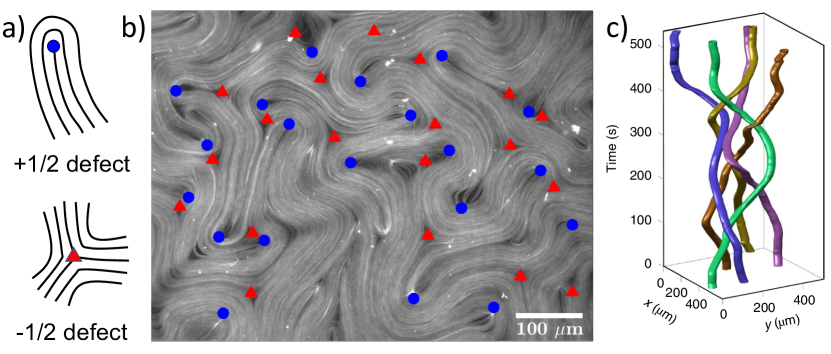
Figure 1: a) Cartoon of defects showing nematic contours. b) Fluorescence image of MT-based active nematic with +1/2 (circles) and -1/2 (triangles) defects. c) Space-time braiding of experimental +1/2 defect positions. (Adapted from Ref. Tan et al., 2019.)

A key goal in active nematics research is to coax them to perform some useful control objective. A natural objective is to optimize their self-mixing, which could have practical benefits in microfluidic systems, where mixing, e.g. of reagents, is particularly difficult due to lack of turbulence Cha . We characterize mixing by the amount of stretching in the fluid, quantified by the topological entropy $h$; in a 2D fluid $h$ equals the asymptotic exponential stretching rate of a passively advected material curve. We seek to maximize this stretching over the natural “active” time scale of the system, defined below.

Reference Tan et al., 2019 first applied topological entropy to active nematics—for the MT-based active nematics, $h$ was computed quite accurately from the space-time “braiding” of +1/2 defects about one another (Fig. 1c). Defects act as virtual rods stirring the fluid. Thus, optimizing mixing reduces to coaxing the +1/2 defects into an efficient braid pattern. Reference Smith and Dunn, 2022 addressed which braid to target, conjecturing, with strong numerical evidence, that the orbit in Fig. 2a maximizes the topological entropy per operation, with $h_{\text{TEPO}}=\log(\phi+\sqrt{\phi})=1.0613$, where $\phi=(1+\sqrt{5})/2$ is the golden ratio. An operation is a set of simultaneous swaps (clockwise or counterclockwise) of neighboring defects. Due to the numerical evidence, we call this the maximal mixing braid.

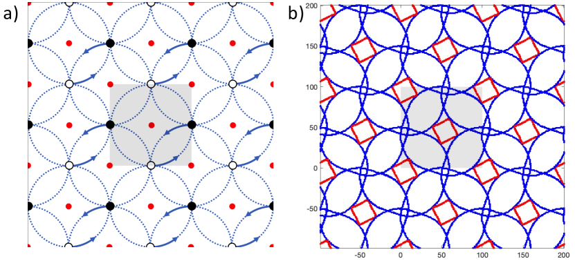
Figure 2: a) Cartoon showing the circular orbits (blue) of the two stirring rods (open and closed black dots) for the maximal mixing braid on a torus, using a periodic tiling of the fundamental cell (grey). b) Trajectories of positive (blue) and negative (red) defects for simulations with $\ell_{a}=3$. The grey rectangle is the original integration domain, which tiles the remainder of the plane.

This Letter reports that the above maximal mixing braiding state spontaneously occurs in simulations of active nematics, when confined to a sufficiently small square with periodic boundary conditions, i.e. a topological torus. Though numerous theoretical Shendruk et al. (2017); Norton et al. (2018); Zhang, Deserno, and Tu (2020); Norton et al. (2020); Samui, Yeomans, and Thampi (2021); Wagner et al. (2022); Smith and Gong (2022) and experimental Keber et al. (2014); Duclos et al. (2017); Opathalage et al. (2019); Hardoüin et al. (2019, 2020, 2022) works have studied 2D active nematics in strongly confined geometries, and others have studied bulk behavior (i.e. weak confinement) in squares with periodic boundary conditions Thampi, Golestanian, and Yeomans (2013); Giomi et al. (2013); Giomi (2015), we know of no prior study systematically exploring the strong confinement limit on a square with periodic boundary conditions.

Following Ref. Giomi, 2015, we model the fluid velocity $\mathbf{u}$ and nematic tensor $\mathsf{Q}=S(\mathbf{n}\otimes\mathbf{n}-\mathsf{I}/2)$, where $S\geq 0$ is the nematic order parameter and $\mathbf{n}$ is the director field; a director is a unit vector with no distinction between head and tail, i.e. $\mathbf{n}$ and $-\mathbf{n}$ are identified. We numerically solve the two nemato-hydrodynamic equations as given in Ref. Giomi, 2015, the first being

$$\frac{D}{Dt}\mathsf{Q}=\frac{\partial}{\partial t}\mathsf{Q}+\mathbf{u}\cdot\mathbf{\nabla}\mathsf{Q}=\lambda S\mathsf{E}+[\mathsf{Q},\mathsf{\omega}]+\gamma^{-1}\mathsf{H},$$ (1)

where $D/Dt$ is the advective derivative, $[,]$ is the commutator, $\mathsf{E}=[(\nabla\mathbf{u})+(\nabla\mathbf{u})^{T}]/2$ is the strain rate tensor, and $\mathsf{\omega}=[(\nabla\mathbf{u})-(\nabla\mathbf{u})^{T}]/2$ is the vorticity tensor. The flow alignment parameter $\lambda$ describes the shape of the mesoscale nematogens. Circular nematogens have $\lambda=0$. Infinitely thin needles have $\lambda=1$, which we use for most of our simulations. (This value of $\lambda$ is very close to that found in Ref. Golden et al., 2023 as well.) The first two terms on the right of Eq. (1) derive from the passive advection of the microtubules. The deviation from this behavior is given by the rotational viscosity $\gamma$ and the molecular tensor

$$\mathsf{H}=-\frac{\delta}{\delta\mathsf{Q}}F_{\text{LdG}}=-\mathsf{Q}(A+C\text{Tr}(\mathsf{Q}^{2}))+K\nabla^{2}\mathsf{Q},$$ (2)

which is the variation of the Landau-de Gennes (LdG) free energy $F_{\text{LdG}}$ with $C=-A>0$. The first term describes the isotropic-nematic phase transition, and the second term derives from the elastic energy, with elastic constant $K$.

The second dynamic equation is Navier-Stokes,

$$\rho\frac{D}{Dt}\mathbf{u}=\rho\left(\frac{\partial}{\partial t}\mathbf{u}+\mathbf{u}\cdot\nabla\mathbf{u}\right)=\rho\nu\nabla^{2}\mathbf{u}+\mathbf{F}-\nabla p,$$ (3)

assuming incompressibility, $\nabla\cdot\mathbf{u}=0$, with constant density $\rho$. The first term on the right is the viscous drag, with viscosity $\nu$, and the third term is the force density due to the pressure $p$. The force density $F_{i}=\nabla_{j}\Pi_{ij}$ comes from the elastic and active stresses $\Pi=\Pi^{E}+\Pi^{A}$, with $\Pi^{E}=-\lambda\mathsf{H}+[\mathsf{Q},\mathsf{H}]$ and $\Pi^{A}=-\alpha\mathsf{Q}$, and where the activity $\alpha$ in the MT system depends on ATP concentration, motor density, and other material properties.

The bulk, i.e. unconfined, material has two length scales, the active length $\ell_{a}=\sqrt{K/\alpha}$ and nematic coherence length $\ell_{n}=\sqrt{K/C}$, which characterize the average defect spacing and defect core size, respectively. Furthermore, the square domain width $L$ determines the confinement. The active time scale is $t_{a}=K/(\alpha\nu)$ and corresponding velocity is $v_{a}=\ell_{a}/t_{a}=\nu\sqrt{\alpha/K}$. The dynamics is determined by five dimensionless parameters: the flow alignment parameter $\lambda$, the Reynolds number $\text{Re}=K/(\rho\nu^{2})$, a dimensionless rotational viscosity $\tilde{\gamma}=\gamma\nu/K$, a LdG parameter $\tilde{C}=C/\alpha=(\ell_{a}/\ell_{n})^{2}$, and the confinement ratio $\ell_{a}/L$. In simulations, we primarily use $\lambda=1$, $\text{Re}=0.01$, $\tilde{\gamma}=50$, $\tilde{C}=9.0$, and vary the confinement through $\ell_{a}$, keeping $L=100$.

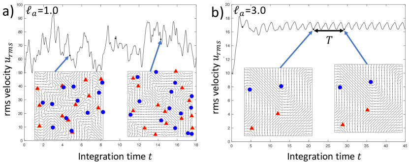
Figure 3: Simulations of active nematics for different values of $\ell_{a}$. a) $\ell_{a}=1.0$. Snapshots of the defect positions and director field are shown along the trace of rms velocity versus time. Defect dynamics is chaotic. b) $\ell_{a}=3.0$. Analogous plot for a more confined case. Defect dynamics is periodic with period $T$.

Fig. 3a shows snapshots of the simulation of Eqs. (1) and (3), with random initial condition, at $\ell_{a}=1.0$. (See Supplemental, movie M1.) Defects are continuously created and destroyed, and their motion is chaotic, as is typical for bulk behavior. The instantaneous root-mean-square (rms) velocity displays a chaotic time dependence. Increasing $\ell_{a}$ to $3.0$ in Fig. 3b confines the system more tightly, with correspondingly fewer defects. (See Supplemental, movie M2.) Unlike the bulk behavior, the rms velocity quickly becomes periodic. Two snapshots taken at the same phase of the motion show essentially the same director field and defect locations. In this periodic state, four defects trace out periodic orbits shown in Fig. 2b, with no creation or annihilation events. A key observation is that the +1/2 orbits are topologically identical to Fig. 2a, showing that the +1/2 defects exhibit the maximal mixing braid. Note that each +1/2 defect traces out a bounded, circular shape. The defects repeatedly encounter and revolve around each other counterclockwise, with four such encounters during each orbit. The -1/2 defects trace out a strikingly square orbit, braiding around no other defects. Of course, by symmetry there is also a reflected orbit in which the +1/2 defects pass each other clockwise.

The maximally mixing orbit is reminiscent of the “Ceilidh dance” orbit, initially observed for channel confinement by Shendruk et al. Shendruk et al. (2017); Samui, Yeomans, and Thampi (2021). In that geometry, the +1/2 defects aggregate along a line with half the defects moving right and the other half left. When opposing defects encounter one another, they alternately pass clockwise and counterclockwise. Several differences distinguish the maximal mixing orbit from the Ceilidh dance: (i) Maximal mixing defects move in a fully 2D pattern; (ii) Defect motion is spatially bounded; (iii) Defects always pass each other in the same sense; (iv) There are no hard-wall boundaries; (v) The orbit generates the maximum topological entropy per operation, $h_{\text{TEPO}}=1.0613$, as conjectured in Ref. Smith and Dunn, 2022, which is strictly larger than that of the Ceilidh dance ($h_{\text{TEPO}}=\log(1+\sqrt{2})=0.8814$) Finn and Thiffeault (2011). Interestingly, the Ceilidh dance is also optimally mixing, but only under the restriction that rods are confined to a linear arrangement Finn and Thiffeault (2011). In a similar manner, it has been shown that the experimental motion of four defects on a sphere Keber et al. (2014) is also very close to maximal mixing for that class of defect braids Smith and Gong (2022). Thus, it would appear that active nematics naturally find maximal mixing states as the system parameters are varied.

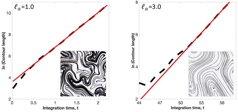
Figure 4: Exponential growth in the contour length for $\ell_{a}=1$ (left) and $\ell_{a}=3$ (right). Insets show final image of advected curves.

To compute topological entropy, we numerically advect an initial line segment forward, recording its length versus time in the semilog plots of Fig. 4, whose slopes yield $h=3.19\pm 0.03$ ($\ell_{a}=1$) and $h=0.475\pm 0.003$ ($\ell_{a}=3$). (See also Supplemental, movies M3 and M4.) Here the units are reciprocal integration time and errors are the error on the mean over four advected curves. Insets show final advected curves. We define a dimensionless topological entropy $\tilde{h}=ht_{a}$, which accounts for the shift in fluid velocity with changing activity, yielding $\tilde{h}=(1.25\pm 0.01)\times 10^{-3}$ ($\ell_{a}=1$) and $\tilde{h}=(1.66\pm 0.01)\times 10^{-3}$ ($\ell_{a}=3$). Thus, by this measure, the periodic motion has more effective mixing by about 33%. Next, we compute the topological entropy from the E-tec (Ensemble-based topological entropy calculation) algorithm Roberts et al. (2019) applied to an ensemble of 1000 randomly initialized advected trajectories. These results agree with the line-stretching computation to within two significant figures: $\tilde{h}=(1.184\pm 0.001)\times 10^{-3}$ ($\ell_{a}=1$) and $\tilde{h}=(1.665\pm 0.003)\times 10^{-3}$ ($\ell_{a}=3$). Since E-tec is more efficient than the line-stretching algorithm (which becomes exponentially more expensive in time), we use E-tec for the remainder of the paper.

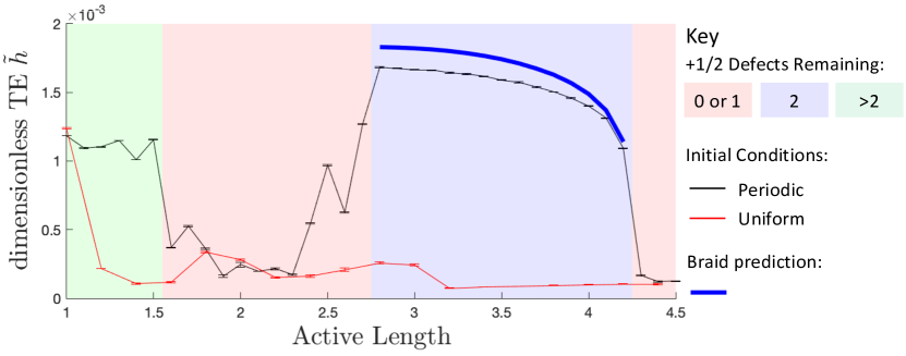
Figure 5: Topological entropy $\tilde{h}$ versus $\ell_{a}$. The initial $\mathsf{Q}$-tensor for black curve is a snapshot of the periodic state at $\ell_{a}=3$, $\tilde{\gamma}=50$, whereas the initial tensor for red curve is nearly constant. Red shading denotes intervals with 0 or 1 +1/2 defects remaining. Blue denotes two remaining and green three or more.

To explore the transition to periodic behavior, Fig. 5 records $\tilde{h}$ for $1\leq\ell_{a}\leq 4.5$. The black curve uses an initial $\mathsf{Q}$-field taken from the periodic state at $\ell_{a}=3$. The system either remains in a nearby stable periodic state or departs from it. The blue band is the interval where the system retains two +1/2 defects for the duration of the simulation. Within this band, the periodic orbit is stable, or at least sufficiently close to stable, that it remains mostly periodic over the course of the simulation. The topological entropy drops precipitously on either side of the blue band, due to the periodic state either disappearing or becoming sufficiently unstable. On either side of the periodic band, the system converges to a steady state with no defects and small, nearly constant, velocity (red band). Technically, for a small number of $\ell_{a}$ values in this interval, a pair of opposite defects remained at the end of the integration, but such a lone pair is expected to eventually annihilate when integrated further. At $\ell_{a}\lesssim 1.5$ the final state has chaotic defect motion with three or more defects (green band) and an intermediate value of $\tilde{h}$.

The dimensionless topological entropy of the maximal mixing braid is $\tilde{h}_{\text{max}}=\log(\phi+\sqrt{\phi})/(\tilde{T}/4)$, where $\tilde{T}$ is the period of defect motion in units of $t_{a}$. This produces the blue curve in Fig. 5, which closely tracks $\tilde{h}$, albeit at a slightly larger value. We attribute this difference to the positive defects moving slightly faster than the surrounding fluid. For example, at $\ell_{a}=3.0$ the rms difference between defect and fluid velocities is about 34%. This fact is also seen by the defect passing through the advected curves. (See Supplemental movies M3 and M4.) This difference in velocity is also seen in experiments as the MT bundles fracturing when bent too far Sanchez et al. (2012).

To clarify the bifurcation at the left edge of the blue band in Fig. 5, we compute the Lyapunov exponent $\Lambda$ of the periodic solution by measuring how quickly a nearby state diverges from it (for positive $\Lambda$) or converges to it (for negative $\Lambda$). See Fig. 6a. The Lyapunov exponent transitions from negative to positive as $\ell_{a}$ decreases, passing through zero at $\ell_{a}=\ell_{c}\approx 2.92$. The linear trend in $\Lambda$ and the fact that no nearby stable periodic orbit exists below $\ell_{c}$, suggests that this is a subcritical pitchfork bifurcation Strogatz (1994) (and certainly not a saddle-node or supercritical pitchfork bifurcation). Pitchfork bifurcations generically occur for systems with a discrete symmetry whose square is the identity, as for certain translational, rotational, and mirror symmetries of Fig. 2b. Thus, we suspect that there is a pair of nearby unstable symmetrically related periodic solutions for $\ell_{a}>\ell_{c}$, which collide with the stable periodic orbit at $\ell_{c}$ to drive it toward instability.

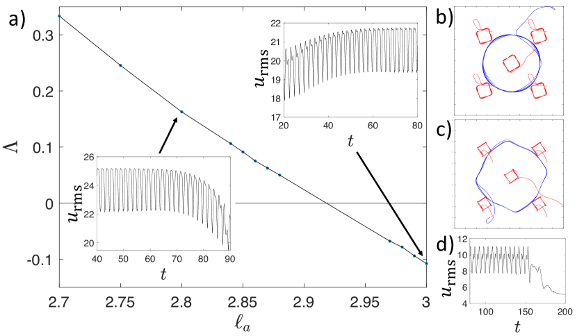
Figure 6: a) The Lyapunov exponent of the periodic orbit. Insets show $u_{\text{rms}}$ vs. integration time for positive and negative $\Lambda$. b) An orbit diverging from the periodic orbit for $\ell_{a}=2.8$. c) Same as (b) for $\ell_{a}=4.15$. d) $u_{\text{rms}}$ vs. time for orbit in (c).

For a given $\ell_{a}<\ell_{c}$, a +1/2 trajectory diverges “adiabatically” from the periodic state. As each +1/2 defect swaps past its partner, it is nudged slightly until it eventually annihilates with a -1/2 defect. (See Fig. 6b and Supplemental movie M5.) Since each nudge is small, the periodic oscillations in $u_{\text{rms}}$ persist, but with a gentle downward trend (left inset of Fig. 6a.) The same trend is seen in reverse for $\ell_{a}>\ell_{c}$, as the nudges stabilize the orbit (right inset of Fig. 6a.)

Unstable orbits near the right edge of the blue band behave very differently (Fig. 6c.) First, the +1/2 orbit has developed four kinks, each coming from a head on collision between the two +1/2 defects. (See Supplemental movie M4.) Eventually, small perturbations lead to a hard scattering event that nearly instantaneously pushes the +1/2 defect onto an entirely different path, causing it to annihilate with a -1/2 defect. The orbit changes “nonadiabatically”; $u_{\text{rms}}$ remains periodic until suddenly breaking down (Fig. 6d).

The active nematic can exhibit bistability, with the final dynamics dependent on the initial conditions. The red curve in Fig. 5 is the entropy $\tilde{h}$ resulting from a nearly uniform initial director field. The bump seen in the black curve due to the maximal mixing orbit is now absent. Furthermore, the jump in entropy due to chaotic trajectories only occurs for the lowest value of $\ell_{a}$.

To understand how the shape of the nematogen affects our results, we varied $\lambda$, keeping $\tilde{\gamma}$, $\tilde{C}$, Re fixed and varying $\ell_{a}$. We found that $\lambda$ needed to be sufficiently large, roughly greater than or equal to 0.6 for the periodic orbit to be visible (Supplemental Fig. 1). We also explored how our results varied with the rotational viscosity $\tilde{\gamma}$. See the Supplemental Material for details.

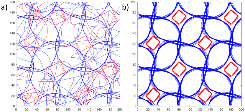
Figure 7: a) Simulation ($\ell_{a}=3$) on a square domain having twice the width as before, with periodic boundary conditions. Maximal mixing solution is no longer stable as seen by negative (red) and positive (blue) defect trajectories. b) Identical simulation except eight control points are added following the negative defects.

Recall that the maximal mixing solution relies on tight confinement within a flat square with periodic boundary conditions; this setup is unphysical in the lab. So, for this solution to be experimentally seen, it would need to be stable when periodically tiled over an experimental domain large enough that boundary effects could be ignored. To test this, we ran simulations on a square with twice the width, using an initial Q-tensor consisting of a 2x2 tiling of the original periodic state plus a small perturbation that breaks the discrete translational symmetry. The computation showed that the periodic solution was unstable (See Fig. 7a and the left side of Supplemental movie M7.) Thus, this periodic motion must be stabilized to be seen in the lab. We focus on a simple method that introduces local control points in the fluid; at a control point, the potential in the LdG free energy inverts at the origin to become a well with a single minimum. This induces a local phase transition to the isotropic state at each control point. (For details on the modification to the LdG free energy, see the Supplement.) Our computations show that these control points indeed successfully stabilize the maximal mixing state (Figure 7b and the right side of Supplemental movie M7.) The simulation in Fig. 7a (without control points) uses exactly the same initial conditions as Fig. 7b (with control points) and runs for the same duration. Thus, we have realized in computation the stabilization of the maximal mixing state over an expanded domain.

The control points need to be dynamic, following square paths that closely track the negative defects in the original periodic orbit. Intuitively, the negative defects nucleate and are trapped in the vicinity of the control points. The positive defects, however, are not directly controlled, but are free to move. Note that the motion of the control points themselves have zero topological braid entropy. All topological entropy, and hence mixing, is generated by the response of the positive defects.

The control points might be realized in the lab in several ways. One basic approach could be to use a laser to interrupt the nematic structure at the control points, analogous to laser-melting of a thermotropic liquid crystal Škarabot et al. (2007); Nikkhou et al. (2015). More generally, a variety of optical techniques have recently been developed to control activity and guide defects Ross et al. (2019); Zhang et al. (2021); Zarei et al. (2023); Lemma et al. (2023). Finally, one might place at the control points a physical obstruction, such as a movable (and ideally controllable, e.g. optically or magnetically) pillar, large bead, or some other floating microfabricated structure, as utilized in Refs. Ray, Zhang, and Dogic, 2023; Rivas et al., 2020.

The periodic behavior demonstrated here thus provides a new possibility for taming the chaos and unpredictability of active nematics, while also enhancing their overall mixing.

We benefitted greatly from discussions with Linda Hirst and members of her lab at UC Merced. This material is based upon work supported by the National Science Foundation under Grant Nos. DMR-1808926, DMR-2225543, and PHY-2150531.

References

- Marchetti et al. (2013) M. C. Marchetti, J. F. Joanny, S. Ramaswamy, T. B. Liverpool, J. Prost, M. Rao, and R. A. Simha, “Hydrodynamics of soft active matter,” Rev. Mod. Phys. 85, 1143–1189 (2013).
- Keber et al. (2014) F. C. Keber, E. Loiseau, T. Sanchez, S. J. DeCamp, L. Giomi, M. J. Bowick, M. C. Marchetti, Z. Dogic, and A. R. Bausch, “Topology and dynamics of active nematic vesicles,” Science 345, 1135–1139 (2014), https://www.science.org/doi/pdf/10.1126/science.1254784 .
- Duclos et al. (2017) G. Duclos, C. Erlenkämper, J.-F. Joanny, and P. Silberzan, “Topological defects in confined populations of spindle-shaped cells,” Nature Physics 13, 58–62 (2017).
- Opathalage et al. (2019) A. Opathalage, M. M. Norton, M. P. N. Juniper, B. Langeslay, S. A. Aghvami, S. Fraden, and Z. Dogic, “Self-organized dynamics and the transition to turbulence of confined active nematics.” Proc Natl Acad Sci U S A 116, 4788–4797 (2019).
- Hardoüin et al. (2019) J. Hardoüin, R. Hughes, A. Doostmohammadi, J. Laurent, T. Lopez-Leon, J. M. Yeomans, J. Ignés-Mullol, and F. Sagués, “Reconfigurable flows and defect landscape of confined active nematics,” Communications Physics 2, 121 (2019).
- Hardoüin et al. (2020) J. Hardoüin, J. Laurent, T. Lopez-Leon, J. Ignés-Mullol, and F. Sagués, “Active microfluidic transport in two-dimensional handlebodies,” Soft Matter 16, 9230–9241 (2020).
- Hardoüin et al. (2022) J. Hardoüin, C. Doré, J. Laurent, T. Lopez-Leon, J. Ignés-Mullol, and F. Sagués, “Active boundary layers in confined active nematics,” Nature Communications 13, 6675 (2022).
- Sanchez et al. (2012) T. Sanchez, D. T. N. Chen, S. J. DeCamp, M. Heymann, and Z. Dogic, “Spontaneous motion in hierarchically assembled active matter,” Nature 491, 431 EP – (2012).
- Henkin et al. (2014) G. Henkin, S. J. DeCamp, D. T. N. Chen, T. Sanchez, and Z. Dogic, “Tunable dynamics of microtubule-based active isotropic gels,” Philosophical Transactions of the Royal Society of London A: Mathematical, Physical and Engineering Sciences 372, 20140142 (2014).
- Giomi (2015) L. Giomi, “Geometry and topology of turbulence in active nematics,” Phys. Rev. X 5, 031003 (2015).
- DeCamp et al. (2015) S. J. DeCamp, G. S. Redner, A. Baskaran, M. F. Hagan, and Z. Dogic, “Orientational order of motile defects in active nematics,” Nature Materials 14, 1110 EP – (2015).
- Guillamat, Ignés-Mullol, and Sagués (2016) P. Guillamat, J. Ignés-Mullol, and F. Sagués, “Control of active liquid crystals with a magnetic field,” Proceedings of the National Academy of Sciences 113, 5498–5502 (2016), https://www.pnas.org/content/113/20/5498.full.pdf .
- Doostmohammadi et al. (2017) A. Doostmohammadi, T. N. Shendruk, K. Thijssen, and J. M. Yeomans, “Onset of meso-scale turbulence in active nematics,” Nature Communications 8, 15326 EP – (2017).
- Guillamat, Ignés-Mullol, and Sagués (2017) P. Guillamat, J. Ignés-Mullol, and F. Sagués, “Taming active turbulence with patterned soft interfaces,” Nature Communications 8, 564 (2017).
- Shendruk et al. (2017) T. N. Shendruk, A. Doostmohammadi, K. Thijssen, and J. M. Yeomans, “Dancing disclinations in confined active nematics,” Soft Matter 13, 3853–3862 (2017).
- Doostmohammadi et al. (2018) A. Doostmohammadi, J. Ignés-Mullol, J. M. Yeomans, and F. Sagués, “Active nematics,” Nature Communications 9, 3246 (2018).
- Lemma et al. (2019) L. M. Lemma, S. J. DeCamp, Z. You, L. Giomi, and Z. Dogic, “Statistical properties of autonomous flows in 2d active nematics,” Soft Matter 15, 3264–3272 (2019).
- Tan et al. (2019) A. J. Tan, E. Roberts, S. A. Smith, U. A. Olvera, J. Arteaga, S. Fortini, K. A. Mitchell, and L. S. Hirst, “Topological chaos in active nematics,” Nature Physics 15 (2019), 10.1038/s41567-019-0600-y.
- Zhang, Mozaffari, and de Pablo (2021) R. Zhang, A. Mozaffari, and J. J. de Pablo, “Autonomous materials systems from active liquid crystals,” Nature Reviews Materials 6, 437–453 (2021).
- Doostmohammadi and Ladoux (2022) A. Doostmohammadi and B. Ladoux, “Physics of liquid crystals in cell biology,” Trends in Cell Biology 32, 140–150 (2022).
- Alert, Casademunt, and Joanny (2022) R. Alert, J. Casademunt, and J.-F. Joanny, “Active turbulence,” Annual Review of Condensed Matter Physics 13, 143–170 (2022), https://doi.org/10.1146/annurev-conmatphys-082321-035957 .
- (22) See the special journal issue: Phil. Trans. Royal Soc. A 362 (2004), including the overview by S. Wiggins and J. M. Ottino, pg. 937.
- Smith and Dunn (2022) S. A. Smith and S. Dunn, “Topological entropy of surface braids and maximally efficient mixing,” SIAM Journal on Applied Dynamical Systems 21, 1209–1244 (2022).
- Norton et al. (2018) M. M. Norton, A. Baskaran, A. Opathalage, B. Langeslay, S. Fraden, A. Baskaran, and M. F. Hagan, “Insensitivity of active nematic liquid crystal dynamics to topological constraints,” Phys. Rev. E 97, 012702 (2018).
- Zhang, Deserno, and Tu (2020) Y.-H. Zhang, M. Deserno, and Z.-C. Tu, “Dynamics of active nematic defects on the surface of a sphere,” Phys. Rev. E 102, 012607 (2020).
- Norton et al. (2020) M. M. Norton, P. Grover, M. F. Hagan, and S. Fraden, “Optimal control of active nematics,” Phys. Rev. Lett. 125, 178005 (2020).
- Samui, Yeomans, and Thampi (2021) A. Samui, J. M. Yeomans, and S. P. Thampi, “Flow transitions and length scales of a channel-confined active nematic,” Soft Matter 17, 10640–10648 (2021).
- Wagner et al. (2022) C. G. Wagner, M. M. Norton, J. S. Park, and P. Grover, “Exact coherent structures and phase space geometry of preturbulent 2d active nematic channel flow,” Phys. Rev. Lett. 128, 028003 (2022).
- Smith and Gong (2022) S. A. Smith and R. Gong, “Braiding dynamics in active nematics,” Frontiers in Physics 10 (2022), 10.3389/fphy.2022.880198.
- Thampi, Golestanian, and Yeomans (2013) S. P. Thampi, R. Golestanian, and J. M. Yeomans, “Velocity correlations in an active nematic,” Phys. Rev. Lett. 111, 118101 (2013).
- Giomi et al. (2013) L. Giomi, M. J. Bowick, X. Ma, and M. C. Marchetti, “Defect annihilation and proliferation in active nematics,” Phys. Rev. Lett. 110, 228101 (2013).
- Golden et al. (2023) M. Golden, R. O. Grigoriev, J. Nambisan, and A. Fernandez-Nieves, “Physically informed data-driven modeling of active nematics,” Science Advances 9, eabq6120 (2023), https://www.science.org/doi/pdf/10.1126/sciadv.abq6120 .
- Finn and Thiffeault (2011) M. D. Finn and J.-L. Thiffeault, “Topological optimization of rod-stirring devices,” SIAM Review 53, 723–743 (2011).
- Roberts et al. (2019) E. Roberts, S. Sindi, S. A. Smith, and K. A. Mitchell, “Ensemble-based topological entropy calculation (e-tec),” Chaos: An Interdisciplinary Journal of Nonlinear Science 29, 013124 (2019), https://doi.org/10.1063/1.5045060 .
- Strogatz (1994) S. H. Strogatz, Nonlinear dynamics and chaos : with applications to physics, biology, chemistry, and engineering (Perseus, Cambridge, MA, 1994).
- Škarabot et al. (2007) M. Škarabot, M. Ravnik, S. Žumer, U. Tkalec, I. Poberaj, D. Babič, N. Osterman, and I. Muševič, “Two-dimensional dipolar nematic colloidal crystals,” Phys. Rev. E 76, 051406 (2007).
- Nikkhou et al. (2015) M. Nikkhou, M. Škarabot, S. Čopar, M. Ravnik, S. Žumer, and I. Muševič, “Light-controlled topological charge in a nematic liquid crystal,” Nature Physics 11, 183–187 (2015).
- Ross et al. (2019) T. D. Ross, H. J. Lee, Z. Qu, R. A. Banks, R. Phillips, and M. Thomson, “Controlling organization and forces in active matter through optically defined boundaries,” Nature 572, 224–229 (2019).
- Zhang et al. (2021) R. Zhang, S. A. Redford, P. V. Ruijgrok, N. Kumar, A. Mozaffari, S. Zemsky, A. R. Dinner, V. Vitelli, Z. Bryant, M. L. Gardel, and J. J. de Pablo, “Spatiotemporal control of liquid crystal structure and dynamics through activity patterning,” Nature Materials 20, 875–882 (2021).
- Zarei et al. (2023) Z. Zarei, J. Berezney, A. Hensley, L. Lemma, N. Senbil, Z. Dogic, and S. Fraden, “Light-activated microtubule-based 2d active nematic,” (2023), arXiv:2303.02945 [cond-mat.soft] .
- Lemma et al. (2023) L. M. Lemma, M. Varghese, T. D. Ross, M. Thomson, A. Baskaran, and Z. Dogic, “Spatio-temporal patterning of extensile active stresses in microtubule-based active fluids,” PNAS Nexus 2, pgad130 (2023), https://academic.oup.com/pnasnexus/article-pdf/2/5/pgad130/51001919/pgad130.pdf .
- Ray, Zhang, and Dogic (2023) S. Ray, J. Zhang, and Z. Dogic, “Rectified rotational dynamics of mobile inclusions in two-dimensional active nematics,” Phys. Rev. Lett. 130, 238301 (2023).
- Rivas et al. (2020) D. P. Rivas, T. N. Shendruk, R. R. Henry, D. H. Reich, and R. L. Leheny, “Driven topological transitions in active nematic films,” Soft Matter 16, 9331–9338 (2020).