Entropy production and fluctuation theorems for monitored
quantum systems under imperfect detection

Abstract

The thermodynamic behavior of Markovian open quantum systems can be described at the level of fluctuations by using continuous monitoring approaches. However, practical applications require assessing imperfect detection schemes, where the definition of main thermodynamic quantities becomes subtle and universal fluctuation relations are unknown. Here we fill this gap by deriving a universal fluctuation relation that links entropy production in ideal and in inefficient monitoring setups. This provides a suitable estimator of dissipation using imperfect detection records that lower bounds the underlying entropy production at the level of single trajectories. We illustrate our findings with a driven-dissipative two-level system following quantum jump trajectories.

Introduction.— Open quantum systems are subjected to interactions with the environment that can notably alter their properties and evolution from both informational and thermodynamical points of view [1, 2]. The noisy character of energy and matter exchanges can be accessed through the application of indirect quantum measurement schemes that monitor system observables or fluxes continuously in time [3, 4, 5, 6, 7]. The output records reveal information about quantum and thermal fluctuations beyond the density matrix approach and allows the extension of concepts in nonequilibrium stochastic thermodynamics to the quantum realm [8, 9, 10, 11, 12, 13, 14, 15, 16, 17, 18, 19, 20, 21, 22, 23, 24] (for a recent review see Ref. [25]). Within this context, a crucial result encoding the fluctuating behavior of thermodynamic quantities is the fluctuation theorem (FT),

$$\langle e^{-S_{\mathrm{tot}}}\rangle=1,$$ (1)

where $S_{\mathrm{tot}}$ is the total stochastic entropy production in the ideal monitored setting [see Eq.(6) below] and $\langle\cdot\rangle$ denotes the ensemble average over records [26, 25, 27]. As corollary, the FT above implies the second-law inequality $\langle S_{\mathrm{tot}}\rangle\geq 0$. Moreover, beyond the FT (1), quantum versions of other related universal results have been also obtained in Markovian open quantum systems, such as the thermodynamic and kinetic uncertainty relations [28, 29, 30, 31, 32], or the martingale theory for entropy production [33, 34]. Altogether they provide new insights on the operation of quantum heat engines [35, 36, 37], feedback control scenarios [38, 39, 40, 41, 42] or information erasure [43, 44].

Although any Markovian open quantum system modeled by the Lindblad master equation could be interpreted as monitored by its environment [2], on the practical side, the actual accessible measurements in the laboratory are always imperfect, unavoidably leading to information losses [45, 46, 47, 48, 49] (see Fig. 1). Despite the practical importance of such circumstances, little is still known about how thermodynamic quantities can be estimated by using only partially accessible information from the measurement records or what universal properties their fluctuations should verify if any [50, 51, 52, 53, 54]. These are questions of crucial importance in order to assess the energetic costs of quantum computation and other quantum technologies [55], as well as for designing and interpreting experiments on quantum thermodynamics in driven dissipative systems, or in setups with different thermal contacts.

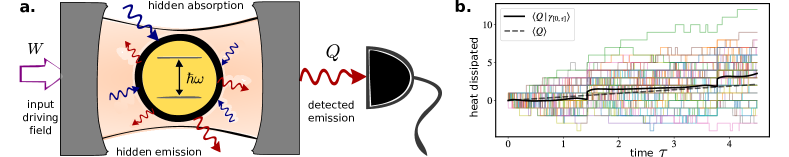
Figure 1: a) Sketch illustrating imperfect detection for a driven two-level atom in an optical cavity. b) Samples of heat dissipated as a function of time conditioned on given set of (two) detected events together with their conditional average $\langle Q|\gamma_{[0,\tau]}\rangle$ (black thick line) and the standard average $\langle Q\rangle$ predicted by the Lindblad master equation (grey dashed line).

In this Letter we extend the thermodynamics of quantum monitored system to partial and imperfect detection. In particular, we introduce a generic irreversibility estimator $\Sigma$ based on measurement records $\gamma_{[0,t]}$ obtained under imperfect monitoring of the open system up to time $t$, and show that it provides a faithful estimation of the minimal dissipation incurred in generic Markovian processes. This result derives from the following central fluctuation relation:

$$e^{-\Sigma}=\langle e^{-S_{\mathrm{tot}}}|\gamma_{[0,t]}\rangle,$$ (2)

where $\Sigma$ will be specified below [see Eq.(7)], and $\langle\cdot|\gamma_{[0,t]}\rangle$ is the conditional average for a given fixed imperfect record. The above fluctuation theorem generalizes the known result on irreversibility in ideal conditions to the imperfect detection scenario and implies, by means of Jensen’s inequality for conditional expectations, the inequality:

$$\Sigma\leq\langle S_{\mathrm{tot}}|\gamma_{[0,t]}\rangle,$$ (3)

which allows us to interpret $\Sigma$ as a (trajectory) estimator lower-bounding stochastic entropy production when the record $\gamma_{[0,t]}$ is observed. Taking the ensemble average of the above equation over many records, we obtain $\langle\Sigma\rangle\leq\langle S_{\mathrm{tot}}\rangle$, providing a lower bound on the average dissipation of the monitored process, but also $\langle\Sigma^{k}\rangle\leq\langle S_{\mathrm{tot}}^{k}\rangle$ for all even powers ($k=2,4,\dots$). In the following, we provide details on how Eqs. (2) and (3) are obtained, together with other related results deriving from them, and discuss their physical interpretation and implications. Detailed proofs are given in the Supplemental Material  [56].

Model.— We consider Markovian open quantum systems weakly interacting with one or several thermal reservoirs, whose evolution is described by the Lindblad master equation ($\hbar=k_{B}=1$):

$$\dot{\rho_{t}}=\mathcal{L}(\rho_{t})=-i[H,\rho_{t}]+\sum_{k=1}^{K}\mathcal{D}[L_{k}]\rho_{t},$$ (4)

where $\rho_{t}$ is the density operator of the system, $H$ its Hamiltonian, and $\mathcal{D}[L]\rho=L\rho L^{\dagger}-\{L^{\dagger}L,\rho\}/2$ a dissipator describing irreversible processes triggered by the environment associated to a set of Lindblad or jump operators $\{L_{k}\}$ (emission and absorption of quanta, dephasing, etc). Importantly both $H$ and $L_{k}$ can be time-dependent, following the externally imposed variation of some parameter $\lambda$ that follows a prescribed control protocol $\Lambda:=\{\lambda(t);0\leq t\leq\tau\}$ up to some final time $\tau$. We assume local detailed balance for the jump operators, i.e. every jump process is related to its inverse counterpart as $L_{\tilde{k}}=L_{k}^{\dagger}e^{-\Delta s_{k}/2}$, which is also included in the set $\{L_{k}\}$ [17]. Here $\Delta s_{k}$ is the entropy change in the environment associated to the $k$th jump .

We further assume the system of interest to be initially prepared at time $t=0$ in a pure state $\ket{n}_{0}$ with probability $p_{n}(0)$, as sampled from $\rho_{0}=\sum_{n}p_{n}(0)\ket{n}\bra{n}_{0}$. Moreover, we introduce a final projective measurement at time $\tau$ on the system using an arbitrary set of rank-1 projectors $\{\ket{m}\bra{m}_{\tau}\}$, that is useful for the thermodynamic description at the level of fluctuations [25].

The dynamics described by the master equation (4) can be unravelled into quantum trajectories by introducing a continuous monitoring scheme [2], where a generalized measurement is performed on the system at every infinitesimal instant of time $dt$, such that $\rho_{t+dt}=\sum_{k}M_{k}\rho_{t}M_{k}^{\dagger}$ with measurement operators verifying $\sum_{k}M_{k}^{\dagger}M_{k}=\openone$. For concreteness, we assume in the following a quantum jump unravelling, although the results derived here are generically valid for other schemes. Within this approach, the system evolution can be described by a sequence of smooth evolution periods intersected by abrupt jumps associated with operators $L_{k}$, occurring at stochastic times. More precisely, we have $M_{k}=\sqrt{dt}L_{k}$ with $k=1...K$, for a detection of a jump of type $k$ in the interval $[t,t+dt]$, and $M_{0}=\openone-iHdt-dt\sum_{k}L_{k}^{\dagger}L_{k}/2$, for no-jumps during $dt$.

The above procedure is known to describe the state of the system conditioned on a given record of jumps detected during the evolution as a pure state $\ket{\psi}_{t}$, following a stochastic Schrödinger equation [2, 3]. Including the initial state and the final projection, we hence define the complete measurement record up to the final time $\tau$ as $\Gamma_{[0,\tau]}:=\{n,(t_{1},k_{1}),(t_{2},k_{2}),...,(t_{J},k_{J}),m\}$, where $J$ jumps have been detected. Taking the average over different measurement records, we recover the evolution described by the master equation (4).

In an ideal setting, each jump in the system trajectory matches a corresponding detection event. However, in any realistic monitoring setup, many jumps might not be detected. Examples comprise prototypical photon emission from cavities with imperfect mirrors [3, 2, 58], Ramsey interferometry in maser-like cavity QED [59, 60], real-time monitoring of tunnelling electrons [61, 62, 63, 64], or circuit QED setups [45, 65]. In such situations, the monitoring scheme needs to be modified to take into account the detection efficiency $\eta_{k}$ of each process $L_{k}$.

As a consequence of informational leakage in the detection, the state of the system conditioned to a given measurement record can no longer be described by a pure state during the stochastic evolution, being instead a mixture modeled by a density matrix $\sigma_{t}$. The evolution of the state under imperfect monitoring follows a stochastic master equation of the form:

$$d\sigma_{t} =-i[H,\sigma_{t}]dt+\sum_{k}\Big{(}dt\leavevmode\nobreak\ (1-\eta_{k})\mathcal{D}[L_{k}]\sigma_{t}$$ (5)

$$+dt\leavevmode\nobreak\ \eta_{k}\mathcal{H}[L_{k}]\sigma_{t}+dN_{k}\leavevmode\nobreak\ \mathcal{J}[\sqrt{\eta_{k}}L_{k}]\sigma_{t}\Big{)},$$

where we introduced the supeoperators $\mathcal{H}[L]\sigma:=\text{Tr}[L^{\dagger}L\sigma]\sigma-\{L^{\dagger}L,\sigma\}/2$ and $\mathcal{J}[L]\sigma:=L\sigma L^{\dagger}/\text{Tr}[L^{\dagger}L\sigma]-\openone$, describing respectively the smooth evolution of the system when no-jumps are detected and the abrupt changes produced by the jumps. Here above the stochastic jumps are incorporated by using Poisson increments $dN_{k}=\{0,1\}$ associated to the number of detected jumps $N_{k}$, which verify $\langle dN_{k}\rangle=\text{Tr}[L_{k}^{\dagger}L_{k}\rho_{t}]dt$ and $dN_{k}dN_{l}=dN_{k}\delta_{k,l}$ [2].

For perfect detection efficiency, $\eta_{k}=1\leavevmode\nobreak\ \forall k=1,...,K$, the second term in the first line of Eq. (5) disappears, and we recover the ideal monitoring case, for which $\sigma_{t}=\ket{\psi}\bra{\psi}_{t}$, and Eq. (5) is equivalent to the stochastic Schrödinger equation as given in [56]. On the other side, for no-detection $\eta_{k}=0\leavevmode\nobreak\ \forall k$, the two last terms vanish and we recover the Lindblad master equation (4). In this sense, Eq. (5) interpolates between these two extremes of getting either complete or zero information about the microscopic processes $L_{k}$.

The stochastic master equation (5) generates imperfect measurement records $\gamma_{[0,\tau]}:=\{n,(t^{\prime}_{1},k^{\prime}_{1}),...,(t^{\prime}_{V},k^{\prime}_{V})\}$ with $V\leq J$ visible jumps, that contain only partial information with respect to the ideal detection case, i.e. $\gamma_{[0,\tau]}\subseteq\Gamma_{[0,\tau]}$. This observation can be made more precise by formally duplicating the original set of $K$ Lindblad operators $\{L_{k}\}$ in two sets corresponding, respectively, to visible processes $\{L_{k}^{\prime}:=\sqrt{\eta_{k}}L_{k}\}$ and their “hidden" counterparts $\{{L}_{k}^{\ast}:=\sqrt{1-\eta_{k}}L_{k}\}$. In this way the full ideal measurement record can be rewritten as $\Gamma_{[0,\tau]}=\{n,(t^{\prime}_{1},k^{\prime}_{1})...,(t^{\prime}_{V},k^{\prime}_{V}),(t^{*}_{1},k^{*}_{1})...,(t^{*}_{H},k^{*}_{H}),m\}$, in terms of both visible $(t^{\prime}_{j},k^{\prime}_{j})$ and hidden $(t^{\ast}_{j},k^{\ast}_{j})$ jumps, with $V+H=J$. That is, $\Gamma_{[0,\tau]}=\gamma_{[0,\tau]}\cup h_{[0,\tau]}$ with $h_{[0,\tau]}:=\{(t^{*}_{1},k^{*}_{1}),...,(t^{*}_{H},k^{*}_{H})\}$ the hidden jumps that the (imperfect) monitoring scheme fails to detect.

Estimating dissipation.— In order to characterize the thermodynamics of monitored processes we employ the total stochastic entropy production, accounting for irreversibility and dissipation at the most general level [27]. In the case of ideally monitored quantum systems it reads [25]:

$$S_{\mathrm{tot}}(\tau)=\ln\frac{\mathbb{P}(\Gamma_{[0,\tau]})}{\tilde{\mathbb{P}}(\tilde{\Gamma}_{[0,\tau]})}=\Delta S_{\mathrm{sys}}(\tau)+\sum_{r=1}^{R}\beta_{r}Q_{r}(\tau),$$ (6)

where $\mathbb{P}(\Gamma_{[0,\tau]})$ is the probability to obtain a measurement record $\Gamma_{[0,\tau]}$ in the original process (under the driving protocol $\Lambda$), and $\tilde{\mathbb{P}}(\tilde{\Gamma}_{[0,\tau]})$ the probability to obtain the time-reversed sequence of (inverse) jumps $\tilde{\Gamma}_{[0,\tau]}$, when the external driving protocol is also time-reversed, i.e. under $\tilde{\Lambda}=\{\lambda(\tau-t);0\leq t\leq\tau\}$. In the second equality we split the entropy production in the stochastic change in system entropy (self-information) $\Delta S_{\mathrm{sys}}(\tau)=-\ln p_{m}(\tau)+\ln p_{n}(0)$ and the total accumulated heat dissipated during the trajectory, with $Q_{r}(\tau)=\int_{0}^{\tau}\sum_{k\in\mathcal{K}_{r}}dN_{k}\Delta s_{k}T_{r}$ the heat transferred into reservoir $r$ at inverse temperature $\beta_{r}=1/T_{r}$, through the associated set of processes $\mathcal{K}_{r}$.

Equation (6) follows from the micro-reversibility of the monitored dynamics at the level of single trajectories [17, 25]. On the other hand, when imperfect detection is considered, information leakages willgenerally hinder micro-reversibility. Nevertheless, we can define an effective indicator of irreversibility as:

$$\Sigma(\tau):=\ln\frac{\mathrm{P}(\gamma_{[0,\tau]})}{\tilde{\mathrm{P}}(\tilde{\gamma}_{[0,\tau]})}=\Delta S_{\mathrm{sys}}(\tau)+\mathcal{S}_{\mathrm{env}}(\tau),$$ (7)

with marginalized path probabilities $\mathrm{P}(\gamma_{[0,\tau]}):=\sum_{h_{[0,\tau]}}\mathbb{P}(\Gamma_{[0,\tau]})$ and $\tilde{\mathrm{P}}(\tilde{\gamma}_{[0,\tau]}):=\sum_{h_{[0,\tau]}}\tilde{\mathbb{P}}(\tilde{\Gamma}_{[0,\tau]})$, obtained by summing over all possible hidden jumps sequences $h_{[0,\tau]}$. Using the fact that probabilities of initial states in both forward and time-reversed processes do not depend on the monitoring efficiencies ${\eta_{k}}$, the second equality in (7) follows from the introduction of the effective entropy exchange with the environment $\mathcal{S}_{\mathrm{env}}(\tau):=\ln[\mathrm{P}(\gamma_{[0,\tau]}|n)/\tilde{\mathrm{P}}(\tilde{\gamma}_{[0,\tau]}|m)]$. Estimators like $\Sigma(\tau)$ can be evaluated from experimental samples of the monitored system or be calculated with the help of the stochastic master equation (5) and its time-reversed counterpart [56], becoming particularly simpler in nonequilibrium steady-state conditions 

The form of $\Sigma$ in Eq. (7) immediately implies its non-negativity on average as $\langle\Sigma(\tau)\rangle=D[\mathrm{P}(\gamma_{[0,\tau]})||\mathrm{P}(\tilde{\gamma}_{[0,\tau]})]\geq 0$ is a Kullback-Leibler divergence between path probabilities [67], in analogy to the classical case [68]. Moreover, an integral fluctuation theorem is verified as $\langle e^{-\Sigma}\rangle=\sum_{\gamma_{[0,\tau]}}\tilde{\mathrm{P}}(\tilde{\gamma}_{[0,\tau]})=1$. However, the relation between $\Sigma$ with actual thermodynamic quantities, and in particular with the underlying entropy production $S_{\mathrm{tot}}$ in Eq. (6) was, so far, unknown. Our main results presented above, Eqs. (2) and (3), provide a clean link between the apparent irreverisibily in the imperfectly monitored process as measured by $\Sigma$ and the underlying (thermodynamic) dissipation as measrued by the total entropy production $S_{\mathrm{tot}}$.

The key ingredient to obtain the coarse-graining fluctuation theorem in Eq. (2) is the use of conditional path probabilities for the hidden jumps with respect to visible ones, namely $\mathrm{P}(h_{[0,\tau]}|\gamma_{[0,\tau]}):=\mathbb{P}(\Gamma_{[0,\tau]})/\mathrm{P}(\gamma_{[0,\tau]})$, which allows us to write conditional averages of arbitrary functionals $X(\Gamma_{[0,\tau]})$ of the full measurement records as $\langle X|\gamma_{[0,\tau]}\rangle=\sum_{h_{[0,\tau]}}\mathrm{P}(h_{[0,\tau]}|\gamma_{[0,\tau]})X(\Gamma_{[0,\tau]})$. The fluctuation theorem (2) can be further rewritten in standard form as $\langle e^{-(S_{\mathrm{tot}}-\Sigma)}|\gamma_{[0,\tau]}\rangle=1$, from which we obtain, inspired by Refs. [69, 70], the following bound relating the fluctuations of $S_{\mathrm{tot}}$ with $\Sigma$:

$$\mathrm{Pr}(S_{\mathrm{tot}}-\Sigma<-\xi)\leq e^{-\xi},$$ (8)

with $\xi\geq 0$. The above inequality implies that the probability of having stochastic entropy production values $S_{\mathrm{tot}}$ below the estimation $\Sigma$ given the visible measurement record $\gamma_{[0,\tau]}$, is exponentially suppressed. In other words, the probability that $\Sigma$ overstimates stochastic entropy production in the monitored thermodynamic process is exponentially negligible.

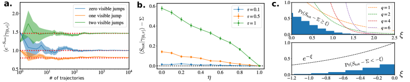
Figure 2: Numerical testing of main results. a) Convergence of fluctuation theorem in Eq. (2) by conditional sampling of $\langle e^{-S_{\mathrm{tot}}}|\gamma_{[0,\tau]}\rangle$ (solid lines) to $e^{-\Sigma}$ (dashed lines) for different three visible trajectories (see legend). Statistical errors are given by shaded areas around the lines. b) Test of inequalities (3) and (10) as a function of detection efficiency $\eta:=\eta_{+}=\eta_{-}$ for a trajectory without visible jumps with different lengths. c) Upper (top) and lower (bottom) statistical bounds on entropy production as a function deviations $\xi$ from Eqs. (9) and (8) respectively. Other parameters: $\Gamma_{0}=10^{-3}\omega$, $\epsilon=10^{-2}\omega$, $\beta\omega=1/5$ and $\hbar\omega=1$ (for all the plots). For (a) $\Gamma_{0}\tau=1$ and $\eta_{+}=\eta_{-}=0.2$. For (c) $\Gamma_{0}\tau=3$, $\eta_{-}=0.5$ and $\eta_{+}=0.2$.

Similarly, we provide a family of bounds for the right tail of $S_{\mathrm{tot}}$ distribution:

$$\mathrm{Pr}(S_{\mathrm{tot}}-\Sigma\geq\xi)\leq e^{-q\xi}\langle e^{q(S_{\mathrm{tot}}-\Sigma)}|\gamma_{[0,\tau]}\rangle,$$ (9)

with again $\xi\geq 0$. In the limit of large trajectories, $\tau\rightarrow\infty$, the right hand side of the above inequality can be minimized [71] for $q=1$, leading to $\mathrm{Pr}(S_{\mathrm{tot}}\geq\Sigma+\xi)\leq e^{-\xi}e^{\tau K(1)}$, with $K(q):=\lim_{\tau\rightarrow\infty}\ln\langle e^{q(S_{\mathrm{tot}}(\tau)-\Sigma)}|\gamma_{[0,\tau]}\rangle/\tau$ a scaled cumulant generation function [72]. The above Eq. (9) and its long time limit thus provide us precise bounds on how much $S_{\mathrm{tot}}$ may be understimated by $\Sigma$, following an exponential decay on $\xi$, attenuated by the factor $\langle e^{q(S_{\mathrm{tot}}-\Sigma)}|\gamma_{[0,\tau]}\rangle\geq 1$. As a corollary we observe that only if $K(1)\rightarrow 0$ the inequality $\eqref{eq:bound}$ becomes tight for arbitrary large trajectories. For detailed proofs of Eqs. (8) and (9) and the long-time limit, see the supplemental material [56].

The explicit expressions of stochastic entropy production in Eq. (6) and the irreversibility indicator in Eq. (7), allow us to rewrite the bound in Eq. (3) in terms of the heat as:

$$\mathcal{S}_{\mathrm{env}}(\tau)\leq\sum_{r}\beta_{r}\langle Q_{r}(\tau)|\gamma_{[0,\tau]}\rangle,$$ (10)

where $\langle Q_{r}|\gamma_{[0,\tau]}\rangle=\sum_{h_{[0,\tau]}}\mathrm{P}(h_{[0,\tau]}|\gamma_{[0,\tau]})Q_{r}(\tau)$ is the expected heat dissipated into reservoir $r$ given the visible measurement record $\gamma_{[0,\tau]}$. We notice that here $\mathcal{S}_{\mathrm{env}}(\tau)$, as well as $\langle Q_{r}|\gamma_{[0,\tau]}\rangle$ can be either positive or negative (a explicit expression for $\langle Q_{r}(\tau)|\gamma_{[0,\tau]}\rangle$ is given in [56]). However $\mathcal{S}_{\mathrm{env}}(\tau)$ always provides us a lower bound on heat dissipation and hence can be regarded as the minimum (integrated) entropy flow to the environment compatible with observations $\gamma_{[0,\tau]}$. The equality case in Eq. (10), as well as in Eq. (3), is reached for unit efficiencies $\eta_{k}=1\leavevmode\nobreak\ \leavevmode\nobreak\ \forall k$, in which case $\gamma_{[0,\tau]}=\Gamma_{[0,\tau]}$. However, Eq. (10) provides a tight bound on the heat whenever $Q_{r}(\tau)$ remains similar for every possible set of hidden jumps $h_{[0,\tau]}$, as it would be the case e.g. for short times, small energies of the inefficiently detected channels, or high temperatures. It is also worth noticing that by taking the average in Eq. (10) or Eq. (2) over final and (or) initial measurement outcomes $\{m,n\}$, other equalities and inequalities can be obtained that depend only on the detected jumps sequence $\{(t_{1}^{\prime},k_{1}^{\prime}),...,(t^{\prime}_{V},k^{\prime}_{V})\}$ (see [56] for details). Taking the average over the entire records $\gamma_{[0,\tau]}$ we obtain, as expected, $\langle\mathcal{S}_{\mathrm{env}}(\tau)\rangle\leq\sum_{r}\beta_{r}\langle Q_{r}(\tau)\rangle$.

Illustrative example.— To exemplify our results, we have chosen a simple two-level system interacting with a bosonic environment at thermal equilibrium and weakly driven by a resonant coherent field. The Hamiltonian for the two-level system is $H_{0}=\omega\ket{1}\bra{1}$, which exchanges energy quanta with the environment through emission and absorption processes. These are described by the Lindbland operators $L_{-}=\sqrt{\Gamma_{0}(\bar{n}+1})\sigma_{-}$ and $L_{+}=\sqrt{\Gamma_{0}\bar{n}}\sigma_{+}$, where $\sigma_{-}$ and $\sigma_{+}$ are lowering and raising operators, $\Gamma_{0}$ is the spontaneous decay rate, and $\bar{n}$ is the average number of bosons in the reservoir. The driving on the system is described by a time-dependent perturbation to $H_{0}$, namely $V(t)=\epsilon(\sigma_{+}e^{-i\omega t}+\sigma_{-}e^{i\omega t})$, with $\epsilon\ll\omega$, which ensures that the structure of the Lindblad operators is unaffected by the driving.

We focus on steady-state conditions, where the system reaches a nonequilibrium state showing coherence in the energy basis. This state is maintained by the continuous dissipation of input work from the drive as heat into the thermal environment, which is partially monitored (see Fig. 1b). We numerically tested our main fluctuation relations and inequalities by assuming imperfect detection of both emission and absorption processes, with respective efficiencies $\eta_{-}$ and $\eta_{+}$. Quantum trajectories of this system conditioned on visible jumps can be computed from the stochastic master equation Eq. (5), while evaluation of conditional averages requires modifications on the original quantum-trajectory Monte Carlo algorithm [56]. We find an excellent convergence for the fluctuation theorem in Eq. (2) when increasing the number of sampled hidden jump sequences $h_{[0,\tau]}$ for three different fixed (visible) records $\gamma_{[0,\tau]}$(Fig. 2a). In Fig. 2b we show the tightness of the bounds (3) and (10) on the heat dissipated into the environment when modifying the efficiency of detection. As we can see there, the difference $\langle S_{\mathrm{tot}}|\gamma_{[0,\tau]\rangle}-\Sigma=\beta\langle Q|\gamma_{[0,\tau]\rangle}-\mathcal{S}_{\mathrm{env}}$ approaches zero when increasing the efficiency of detection of both emission and absorption events, leading to the saturation of the bound for perfect detection. Moreover, as shown from the different lines, when increasing the length of the trajectories for a fixed visible jump record, this difference becomes greater due to the highest occurrence of hidden jumps. We finally evaluated the statistics of $S_{\mathrm{tot}}$ over hidden jump sequences (Fig. 2c) in order to test the exponential decay bound of entropy production fluctuations below $\Sigma$ predicted by Eq. (8) (bottom plot) and the attenuated decay above $\Sigma$ bounded by the family of curves in Eq. (9) for $q\geq 1$ (top plot).

Concluding remarks.— Our results apply to classical and quantum monitored systems alike. Within the classical context, our results generalize previous results for estimation of average entropy production in non-equilibrium steady-states [73, 74] to the level of single trajectories and fluctuations, which may find applications to energy-transduction in living systems [75, 76, 77, 78], also including situations where only a few transitions between system states can be observed [79, 80]. On the quantum side, while we focused on quantum jump trajectories, the results presented here are general and may be explicitly extended to the case of diffusive dynamics (which can be derived from the quantum jumps approach in a particular limit [2, 3, 81]), an interesting perspective that we leave for future work. We expect that our results will be of relevance in experimental situations aiming to asses quantum thermodynamics [82, 53, 22, 83], finding applications for assessing energetic costs in quantum technologies of the noisy intermediate-scale quantum (NISQ) era [55].

Acknowledgments.— We wish to acknowledge support from the María de Maeztu project (CEX2021-001164-M) for Units of Excellence, QUARESC project (PID2019-109094GB-C21) and QuTTNAQMa project (PID2020-117347GB-I00), funded by the Spanish State Research Agency MCIN/AEI/10.13039/501100011033. RL acknowledges the financial support by the Grant No. PDR2020/12 sponsored by Comunitat Autonoma de les Illes Balears through the ‘Direcció General de Política Universitaria i Recerca’ with funds from the Tourist Stay Tax Law ITS 2017-006 and the Grant No. LINKB20072 from the CSIC i-link program 2021. GM acknowledges funding from Spanish MICINN through the Ramón y Cajal program (RYC2021-031121-I). MFC also acknowledges funding from Generalitat Valenciana (CIACIF/2021/434).

Supplemental Material to “Entropy production and fluctuation theorems for monitored quantum systems under imperfect detection”

The Supplemental Material includes comprehensive proofs of our main results and further elaboration on the ideas introduced in the main text. We initially review some of the basic concepts in the formalism of quantum jump trajectories and the definition of entropy production in such framework, which are crucial in this work in section S1. Then in section S2 we give the detailed proof of the central result of the Letter, that is the fluctuation theorem in Eq. (2), together with inequality (3) there. In section S3 we provide the proofs for the results in Eqs.(8) and (9) of the main text, providing bounds to the entropy production estimation under imperfect detection. Section S4 is devoted to provide details on how the estimator of irreversibility $\Sigma$ can be constructed from detected trajectories, while in section S5 we give an explicit expression for the conditional heat along quantum-jump trajectories of systems subjected to imperfect detection. In section S6 we provide slightly different version of the fluctuation theorem (2) valid when we perform an average over initial and final measurements of the two-point measurement scheme. Section S7 contain details about the example used in the main text to illustrate our results. Finally, in Section S8 we discuss the numerical methods employed to obtain conditional averages using Quantum Monte Carlo simulations.

S1 Entropy production in quantum-jumps trajectories

The unraveling of the master equation in Eq. (4) in the main text by using an ideal direct detection scheme [2], as reported in the main text, leads to the following stochastic Schrödinger equation:

$$d\ket{\psi}_{t}=[-idtH-\frac{dt}{2}\sum_{k}\left(L_{k}^{\dagger}L_{k}-\langle L_{k}^{\dagger}L_{k}\rangle_{\psi}\right)+\sum_{k}dN_{k}\left(\frac{L_{k}}{\sqrt{\langle L_{k}^{\dagger}L_{k}\rangle}_{\psi}}-\mathds{1}\right)]\ket{\psi}_{t}$$ (S1)

where we denoted $\langle L_{k}^{\dagger}L_{k}\rangle_{\psi}=\bra{\psi}_{t}L_{k}^{\dagger}L_{k}\ket{\psi}_{t}$. Here the first two terms proportional to $dt$ generated a smooth evolution associated to the periods when jumps are not detected. On the other hand the last term is proportional to the stochastic Poisson increments $dN_{k}$. When $dN_{k}=1$ this last term produces a sharp change in the stochastic wave function $\ket{\psi}_{t}$ stemming from the occurrence of a quantum jump. The original Lindblad master equation (4) is recovered from Eq. (S1) by taking constructing the evolution of $\ket{\psi}\bra{\psi}_{t}$ and taking the average over possible outcomes of the jumps $\langle dN_{k}\rangle=\text{Tr}[L_{k}^{\dagger}L_{k}\rho_{t}]dt$.

Given an ideal record of $J$ jumps $j_{[0,\tau]}=\{(t_{1},k_{1})...,(t_{J},k_{J})\}$ during an interval $[0,\tau]$, which in this case we assume to be perfectly detected, the associated evolution of the system from an arbitrary initial state $\ket{\psi}_{0}$ up to time $\tau$ can be written as:

$$\ket{\psi}_{t}=\frac{\mathcal{T}(j_{[0,\tau]}}{\sqrt{p_{\Gamma}}}\ket{\psi}_{0},$$ (S2)

where we used the following trajectory evolution operator for the monitored system containing the information for the specific sequence of jump and no-jump periods during the evolution:

$$\mathcal{T}(j_{[0,\tau]})=\mathcal{U}(\tau,t_{J})L_{k_{J}}\leavevmode\nobreak\ ...\leavevmode\nobreak\ \mathcal{U}(t_{2},t_{1})L_{k_{1}}\mathcal{U}(t_{1},0),$$ (S3)

and the normalization $p_{\mathcal{T}}=\text{Tr}[\mathcal{T}\ket{\psi}\bra{\psi}_{0}\mathcal{T}^{\dagger}]$ representing the probability of the given jump sequence $j_{[0,\tau]}$ when starting from the initial state $\ket{\psi}_{0}$. Here above $\mathcal{U}(t_{2},t_{1})=T_{+}{\rm exp}[-i\int_{t_{1}}^{t_{2}}dt(H+i\sum L_{k}^{\dagger}L_{k})]$ is the (non-unitary) evolution operator associated to a period with no jumps between $t_{1}$ to $t_{2}$.

As mentioned in the main text, in order to address the main thermodynamic quantities along trajectories we also introduce a two-point measurement (TPM) scheme in combination with the continuous monitoring scheme [25]. This approach consists of performing projective measurements of arbitrary observables both at the beginning and at the conclusion of the indirectly monitored process. In particular we assume the sysmtem is prepared in a pure state $\ket{n}$ sampling from the initial density operator of the system, $\rho_{0}=\sum_{n}p_{n}(0)\ket{n}\bra{n}_{0}$. This is equivalent to perform an initial projective measurement using a complete set of projectors $\{\Pi_{n}^{0}=\ket{n}\bra{n}_{0}\}$. After that, the evolution of the system proceeds under continuous monitoring until a final time $\tau$, where a second projective measurement is performed in an arbitrary basis using a complete set of projectors $\{\Pi_{m}^{\tau}=\ket{m}\bra{m}_{\tau}\}$ (for simplicity we may consider the basis of $\rho_{\tau}=\sum_{m}p_{m}(\tau)\ket{m}\bra{m}_{\tau}$). Denoting the outcome of the initial measurement as $n$ and the one of the final measurement as $m$, the complete trajectory of the system can be written as $\Gamma_{[0,\tau]}=\{n,(t_{1},k_{1})...,(t_{J},k_{J}),m\}$ and its probability to occur (path probability) reads:

$$\mathbb{P}(\Gamma_{[0,\tau]})=p_{n}(0)\text{Tr}\left[\Pi_{m}^{\tau}\mathcal{T}(j_{[0,\tau]})\Pi_{n}^{0}\mathcal{T}^{\dagger}(j_{[0,\tau]})\right],$$ (S4)

where first term is the probability of sampling $n$ at the beginning, and the second term is the conditional probability to obtain the jump sequence $j_{[0,\tau]}$ and final outcome $m$ in the second projective measurement when starting from $\ket{n}_{0}$.

The definitions of reversibility and its link with entropy production comprise the comparison of the occurrence of trajectories $\Gamma_{[0,\tau]}$ with the occurrende of their time-reversed counterpart $\tilde{\Gamma}_{[0,\tau]}$ when the driving protocol $\Lambda$ is also inverted. Here, it is convenient to introduce the (anti-unitary) time-reversal operator in quantum mechanics, $\Theta$, which basically changes the sign of the odd variables under time-reversal symmetry in the operators to which it is applied. Moreover, in the following to denominate operators in the time-reversed dynamics, we will use a tilde.

The time-reversed or backward process can be defined from the forward one as follows. It starts with the (inverted) final state of the forward process at time $\tau$, namely $\tilde{\rho}_{0}:=\Theta\rho_{\tau}\Theta^{\dagger}=\sum_{m}p_{m}(\tau)\Theta\Pi_{m}^{\tau}\Theta^{\dagger}$ over which a measurement with projectors $\{\Theta\Pi_{m}^{\tau}\Theta^{\dagger}\}$ where outcome $m$ is obtained, then the monitoring procedure is run subjected to the time-reversed driving protocol $\tilde{\Lambda}=\{\lambda(\tau-t);0\leq t\leq\tau\}$ which registers exactly the time-reversed jumps record. Finally the second measurement is performed using projectors $\{\Theta\Pi_{n}^{0}\Theta^{\dagger}\}$ which gives the (inverted) initial state $\Theta\ket{n}_{0}$.

We will denote the complete time-reversed measurement record as $\tilde{\Gamma}_{[0,\tau]}=\{m,(\tau-t_{J},{k}_{J}),...,(\tau-t_{1},{k}_{1}),n\}$, which reproduce the inverse sequence of (inverted) jumps with respect to $j_{[0,\tau]}$ [25]. The trajectory operator associated to the time-reversed trajectory is:

$$\tilde{\mathcal{T}}({j}_{[0,\tau]})=\tilde{\mathcal{U}}(\tau,\tau-t_{1})\tilde{L}_{k_{1}}\leavevmode\nobreak\ ...\leavevmode\nobreak\ \leavevmode\nobreak\ \tilde{\mathcal{U}}(\tau-t_{J-1},\tau-t_{J})\tilde{L}_{k_{J}}\tilde{\mathcal{U}}(\tau-t_{J},0),$$ (S5)

with corresponding time-reversed operators for no-jumps periods and jumps:

$$\tilde{\mathcal{U}}(t_{2},t_{1}) =\Theta\leavevmode\nobreak\ T_{+}e^{i\int_{t_{1}}^{t_{2}}dt(H(\tilde{\lambda})+i\sum L_{k}^{\dagger}L_{k})}\leavevmode\nobreak\ \Theta^{\dagger},$$ (S6)

$$\tilde{L}_{k_{j}} =\Theta L_{k_{j}}^{\dagger}\Theta^{\dagger}e^{-\Delta s_{k}/2}=\Theta L_{\bar{k}_{j}}\Theta^{\dagger}.$$ (S7)

Notice that in the operator for no-jump periods in the time-reversed dynamics the Hamiltonian is now evaluated at value $\tilde{\lambda}(t)=\lambda(\tau-t)$, as it corresponds to the time-reversed driving protocol $\tilde{\Lambda}$. Moreover we notice that the jumps in the time-reversed dynamics correspond to the (inverted) complementary jumps $L_{\tilde{k}_{j}}$ by virtue of the detailed balance relation for operators $L_{\tilde{k}}=L_{k}^{\dagger}e^{-\Delta s_{k}/2}$, and $\Delta s_{k}$ is the entropy change in the environment associated to the kth jump [17, 25].

The path probability for the inverse trajectory then reads:

$$\tilde{\mathbb{P}}(\tilde{j}_{[0,\tau]})=p_{m}(\tau)\leavevmode\nobreak\ \text{Tr}\left[\Theta\Pi_{n}^{0}\Theta^{\dagger}\leavevmode\nobreak\ \tilde{\mathcal{T}}({j}_{[0,\tau]})\leavevmode\nobreak\ \Theta\Pi_{m}^{\tau}\Theta^{\dagger}\leavevmode\nobreak\ \tilde{\mathcal{T}}^{\dagger}({j}_{[0,\tau]})\right].$$ (S8)

Comparing the probability of trajectories in the forward and time-reversed processes we recover the link between irreversibility as measured in theoretic-information terms with thermodynamic entropy production [17]

$$S_{\mathrm{tot}}(\tau)=\ln\frac{\mathbb{P}(\Gamma_{[0,\tau]})}{\tilde{\mathbb{P}}(\tilde{\Gamma}_{[0,\tau]})}=\Delta S_{\mathrm{sys}}(\tau)+\sum_{r}\beta_{r}Q_{r}(\tau),$$ (S9)

where the second equality follows by splitting the entropy production in the stochastic change in system entropy (self-information) $\Delta S_{\mathrm{sys}}(\tau)=-\ln p_{m}(\tau)+\ln p_{n}(0)$ and the entropy exchange with the environment $\sum_{r}\beta_{r}Q_{r}(\tau)=\sum_{j}\Delta s_{k_{j}}$. Assuming thermal reservoirs we obtain $\Delta s_{k}=\beta_{r}\Delta e_{r}$ with $\Delta e_{r}$ the energy transferred to the reservoir $r$ in the jump $k\in\mathcal{K}_{r}$ pertaining to the set of jumps induced by that reservoir.

S2 Proof of the main fluctuation theorem and inequalities

In the following we provide a proof of the main fluctuation theorem in Eq. (2) of the main text:

$$\langle e^{-S_{\mathrm{tot}}(\tau)}|\gamma_{[0,\tau]}\rangle=\sum_{h_{[0,\tau]}}\mathrm{P}(h_{[0,\tau]}|\gamma_{[0,\tau]})\frac{\tilde{\mathbb{P}}(\tilde{\Gamma}_{[0,\tau]})}{\mathbb{P}(\Gamma_{[0,\tau]})}=\sum_{h_{[0,\tau]}}\frac{\tilde{\mathbb{P}}(\tilde{\Gamma}_{[0,\tau]})}{\mathrm{P}(\gamma_{[0,\tau]})}=\frac{\tilde{\mathrm{P}}(\tilde{\gamma}_{[0,\tau]})}{\mathrm{P}(\gamma_{[0,\tau]})}=e^{-\Sigma(\tau)},$$ (S10)

where in the second line we used $\mathrm{P}(h_{[0,\tau]}|\gamma_{[0,\tau]})=\mathbb{P}(\Gamma_{[0,\tau]})/\mathrm{P}(\gamma_{[0,\tau]})$, then we performed the marginalization over sequences of hidden jumps $\sum_{h_{[0,\tau]}}\tilde{\mathbb{P}}(\tilde{\Gamma}_{[0,\tau]})=\tilde{\mathrm{P}}(\tilde{\gamma}_{[0,\tau]})$, and in the last equality we identified the irreversibility indicator $\Sigma(\tau)=\log[\mathrm{P}(\gamma_{[0,\tau]})/\tilde{\mathrm{P}}(\tilde{\gamma}_{[0,\tau]})]$ as defined in Eq. (7) of the main text. The above equation is identical to Eq. (2) in the main text.

We now apply Jensen’s inequality for conditional averages, namely, $f(\langle X|\gamma_{[0,\tau]})\leq\langle f(X)|\gamma_{[0,\tau]}\rangle$ for any convex function $f(x)$ and trajectory functional $X(\Gamma_{[0,\tau]})$. For the case $f(x)=e^{-x}$ with $x=S_{\mathrm{tot}}-\Sigma$, we obtain:

$$e^{-\langle S_{\mathrm{tot}}-\Sigma|\gamma_{[0,\tau]}\rangle}\leq\langle e^{-S_{\mathrm{tot}}+\Sigma}|\gamma_{[0,\tau]}\rangle=1\leavevmode\nobreak\ \leavevmode\nobreak\ \Leftrightarrow\leavevmode\nobreak\ \leavevmode\nobreak\ \langle S_{\mathrm{tot}}|\gamma_{[0,\tau]}\rangle-\Sigma\geq 0,$$ (S11)

which follows by just taking logarithms at both sides of the inequality and multiplying them by $-1$. Finally, taking the average over all visible trajectories $\gamma_{[0,\tau]}$ we further obtain the inequality:

$$\langle S_{\mathrm{tot}}\rangle\geq\langle\Sigma\rangle\geq 0,$$ (S12)

which can be interpreted as a stronger version of the second-law inquality $\langle S_{\mathrm{tot}}\rangle\geq 0$. Here the inequality $\langle\Sigma\rangle\geq 0$ follows from the fact that $\langle\Sigma\rangle$ can be written as a Kullback-Leibler divergence for the path probabilities of visible trajectories, see main text and Section S4 below.

Finally, the above inequality can be extended to higher moments of $S_{\mathrm{tot}}$ and $\Sigma$. This follows by applying Jensen’s inequality for contidional averages with $f(x)=[-\ln(x)]^{k}$, which is convex for even powers $k=2,4,6,...$ and take $x=e^{-S_{\mathrm{tot}}}$. This yields:

$$\langle S_{\mathrm{tot}}^{k}|\gamma_{[0,\tau]}\rangle\geq[-\ln\langle e^{-S_{\mathrm{tot}}}|\gamma_{[0,\tau]}\rangle]^{k}=[-\ln e^{-\Sigma}]^{k}=\Sigma^{k},$$ (S13)

where we have used the above fluctuation theorem [Eq.(2) in the main text]. This in turns imply, by taking averages over visible trajectories $\gamma_{[0,\tau]}$ that:

$$\langle S_{\mathrm{tot}}^{k}\rangle\geq\langle\Sigma^{k}\rangle\geq 0,$$ (S14)

for all even $k$. This relations ensures that not only the average, but all even moments of the total entropy production distribution are lower-bounded by those of the estimator $\Sigma$.

S3 Proof of statistical bounds on entropy production estimation.

Here we provide the proofs for out statistical bounds for the maximum and minimum of the differences $S_{\mathrm{tot}}-\Sigma$ reported in Eqs. (8) and (9) of the main text. For the proof these inequalities , we first introduce the conditional probability distribution for entropy production, given a set of visible jumps $\gamma_{[0,\tau]}$ as:

$$\mathrm{Pr}(S_{\mathrm{tot}}|\gamma_{[0,\tau]}):=\int_{-\infty}^{\infty}dS_{\mathrm{tot}}\sum_{h_{[0,\tau]}}P(h_{[0,\tau]}|\gamma_{[0,\tau]})\leavevmode\nobreak\ \delta\left(S_{\mathrm{tot}}-\ln\frac{\mathbb{P}(\Gamma_{[0,\tau]})}{\tilde{\mathbb{P}}(\tilde{\Gamma}_{[0,\tau]})}\right),$$ (S15)

where $\delta(x)$ denotes the Dirac delta function. The first inequality [Eq. (8)] lower bounding deviations of the average entropy production conditioned on a measurement record from the estimator $\Sigma$ is obtained by closely following the derivations in Refs. [70, 69] as follows:

$$\mathrm{Pr}(S_{\mathrm{tot}}-\Sigma<-\xi)=\mathrm{Pr}(S_{\mathrm{tot}}<\Sigma-\xi)=\int_{-\infty}^{\Sigma-\xi}dS_{\mathrm{tot}}\leavevmode\nobreak\ \mathrm{Pr}(S_{\mathrm{tot}}|\gamma_{[0,\tau]})$$

$$\leq\int_{-\infty}^{\Sigma-\xi}dS_{\mathrm{tot}}\leavevmode\nobreak\ \mathrm{Pr}(S_{\mathrm{tot}}|\gamma_{[0,\tau]})\leavevmode\nobreak\ e^{-S_{\mathrm{tot}}+\Sigma-\xi}=e^{\Sigma-\xi}\int_{-\infty}^{\Sigma-\xi}dS_{\mathrm{tot}}\leavevmode\nobreak\ \mathrm{Pr}(S_{\mathrm{tot}}|\gamma_{[0,\tau]})e^{-S_{\mathrm{tot}}}$$

$$\leq e^{\Sigma-\xi}\int_{-\infty}^{\infty}dS_{\mathrm{tot}}\leavevmode\nobreak\ \mathrm{Pr}(S_{\mathrm{tot}}|\gamma_{[0,\tau]})e^{-S_{\mathrm{tot}}}=e^{\Sigma-\xi}\langle e^{-S_{\mathrm{tot}}(\tau)}|\gamma_{[0,\tau]}\rangle=e^{-\xi},$$ (S16)

where in the first inequality we used that $S_{\mathrm{tot}}<\Sigma-\xi$ inside the integral limits, and the fluctuation theorem Eq.(1) in the main text for the last equality, and we recall that here $\xi\geq 0$.

Analogously the proof of the upper bound in Eq. (9) follows as:

$$\mathrm{Pr}(S_{\mathrm{tot}}-\Sigma\geq\xi)=\mathrm{Pr}(S_{\mathrm{tot}}\geq\Sigma+\xi)=\int_{\Sigma+\xi}^{\infty}dS_{\mathrm{tot}}\leavevmode\nobreak\ \mathrm{Pr}(S_{\mathrm{tot}}|\gamma_{[0,\tau]})$$

$$\leq\int_{\Sigma+\xi}^{\infty}dS_{\mathrm{tot}}\leavevmode\nobreak\ \mathrm{Pr}(S_{\mathrm{tot}}|\gamma_{[0,\tau]})\leavevmode\nobreak\ e^{q(S_{\mathrm{tot}}-\Sigma-\xi)}\leq e^{-q\xi}\int_{-\infty}^{\infty}dS_{\mathrm{tot}}\leavevmode\nobreak\ \mathrm{Pr}(S_{\mathrm{tot}}|\gamma_{[0,\tau]})e^{q(S_{\mathrm{tot}}-\Sigma)}$$

$$=e^{-q\xi}\langle e^{q(S_{\mathrm{tot}}-\Sigma)}|\gamma_{[0,\tau]}\rangle,$$ (S17)

where we have used that $S_{\mathrm{tot}}\geq\Sigma+\xi$ inside the integration interval and hence $qS_{\mathrm{tot}}\geq q(\Sigma+\xi)$ for $q\geq 1$, after wich we extended the integration interval to the left and identified the conditional average $\langle e^{q(S_{\mathrm{tot}}-\Sigma)}|\gamma_{[0,\tau]}\rangle$. Recall that again here we assumed $\xi\geq 0$.

From the application of Jensen’s inequality (see Sec. S2) for the family of convex functions $f(x)=x^{-q}$ with $q\geq 1$ to the fluctuation theorem in Eq.(1), we obtain that

$$\langle e^{q(S_{\mathrm{tot}}-\Sigma)}|\gamma_{[0,\tau]}\rangle\geq 1,$$ (S18)

which provides a set of inequalities ensuring that the upper bound in Eq. (9) scales generally slower than an exponential.

From the large deviation principle [72] we obtain by taking the long time limit:

$$\lim_{\tau\rightarrow\infty}\langle e^{q\tau(\frac{S_{\mathrm{tot}}-\Sigma}{\tau})}|\gamma_{[0,\tau]}\rangle\simeq e^{\tau K(q)}$$ (S19)

with the escaled cumulant generting function $K(q):=\lim_{\tau\rightarrow\infty}\ln\langle e^{q(S_{\mathrm{tot}}(\tau)-\Sigma)}|\gamma_{[0,\tau]}\rangle/\tau$. That allow us to minimize the upper bound in Eq. (9) over $q$ in the long time limit:

$$\mathrm{Pr}(S_{\mathrm{tot}}-\Sigma\geq\xi)\leq\min_{q}e^{-q\xi}e^{\tau K(q)}=e^{-\xi}e^{\tau K(1)},$$ (S20)

where in the last equality we obtained $q=1$ from the fact that $K(q)\geq 0$ for $q\geq 1$ and that $K(q)$ is convex, as reported in the main text.

S4 Irreversibility estimator from visible trajectories

Here we show how the estimator of irreversibility along visible trajectories $\Sigma(\gamma_{[0,\tau]})$ can be obtained by explicitly calculating the probability of visible trajectories in the forward and time-reversed dynamics. In the case of imperfect detectors leading to hidden jumps during the evolution, the state of the system conditioned to a given measurement record $\gamma_{[0,\tau]}$ can be obtained from the stochastic master equation (5) in the main text, which follows by a coarse-graining of outcomes in the ideal measurement scheme constructed for infinitesimal time-steps of the evolution.

When a (visible) jump is detected, the evolution of the imperfectly monitored system state becomes, up to a normalization factor:

$$\bar{\sigma}_{t+dt}=\eta_{k}M_{k}\rho M_{k}^{\dagger}={\eta_{k}}L_{k}{\sigma_{t}}L_{k}^{\dagger}dt=:\mathcal{J}_{k}(\sqrt{\eta}_{k}{\sigma_{t}})dt,$$ (S21)

where we used the measurement operators for a jump $M_{k}=\sqrt{dt}L_{k}$ as in the ideal case, and used an overbar over the state, $\bar{\sigma}$, to remark that this state is not normalized. On the other hand the evolution during a step of time in which no jumps are detected is now given by an statistical combination of the no-jump evolution and the possibility that a hidden jump occurs, that is

$$\bar{\sigma}_{t+dt}=M_{0}\sigma_{t}M_{0}^{\dagger}+\sum_{k}(1-\eta_{k})M_{k}\sigma_{t}M_{k}^{\dagger}=:{\sigma}_{t}+dt\mathcal{L_{\ast}}({\sigma}_{t})+O(dt^{2}),$$ (S22)

where we have introduced the superoperator:

$$\mathcal{L}_{\ast}(\sigma):=-i\left[H,\sigma\right]-\frac{1}{2}\sum_{k}\left\{L_{k}^{\dagger}L_{k},\sigma\right\}+\sum_{k}(1-\eta_{k})L_{k}\sigma L_{k}^{\dagger},$$ (S23)

which includes the contributions of both no-jumps (second term) and hidden jumps (third term).

Given a visible measurement record $v_{[0,\tau]}=\{(t^{\prime}_{1},k^{\prime}_{1}),...,(t^{\prime}_{V},k^{\prime}_{V})\}$ with $V\leq J$ and some arbitrary initial state $\sigma_{0}$, one can recover the (unnormalized) state by sequential application of the above two evolution operators:

$$\bar{\sigma}(\tau)=\mathcal{N}_{\tau,t_{V}}\circ\mathcal{J}_{k_{V}}\circ\leavevmode\nobreak\ ...\leavevmode\nobreak\ \circ\mathcal{J}_{k_{1}}\circ\mathcal{N}_{t_{1},t_{0}}(\sigma_{0}),$$ (S24)

where $\mathcal{N}_{t_{2},t_{1}}(\sigma):=T_{+}\exp[\int_{t_{1}}^{t_{2}}dt\mathcal{L}_{\ast}](\sigma)$ and we denoted by $A\circ B(\sigma)=A(B(\sigma))$ the convolution of superoperators. Notice that in this case we cannot define trajectory operators as in the ideal case. This is a manifestation of the breakdown of microscopic reversibility within the trajectories [25].

The complete path probability of a visible trajectory given the measurement record $\gamma_{[0,\tau]}$ (including initial and final projective measurement outcomes) is then:

$$\mathrm{P}(\gamma_{[0,\tau]})=p_{n}(0)\leavevmode\nobreak\ \text{Tr}\left[\Pi_{m}^{\tau}\mathcal{N}_{\tau,t_{V}}\circ\mathcal{J}_{k_{V}}\circ...\circ\mathcal{J}_{k_{1}}\circ\mathcal{N}_{t_{1},t_{0}}(\Pi_{n}^{0})\right],$$ (S25)

to be compared with the ideal case in Eq. (S4). Analogously to the ideal case, the probability of the time-reversed visible trajectory is given by:

$$\tilde{\mathrm{P}}(\tilde{\gamma}_{[0,\tau]})=p_{m}(\tau)\leavevmode\nobreak\ \text{Tr}\left[\Theta\Pi_{n}^{0}\Theta^{\dagger}\tilde{\mathcal{N}}_{0,\tau-t_{V}}\circ\tilde{\mathcal{J}}_{k_{1}}\circ...\circ\tilde{\mathcal{J}}_{k_{V}}\circ\tilde{\mathcal{N}}_{\tau-t_{V},0}(\Theta\Pi_{m}^{\tau}\Theta^{\dagger})\right],$$ (S26)

where we used the time-reversed versions of the superoperators in both jump intervals and smooth evolution periods:

$$\tilde{\mathcal{J}}_{k}({\sigma}):=\eta_{k}\tilde{L}_{k}\sigma\tilde{L}_{k}^{\dagger}={\eta_{k}}L_{k}^{\dagger}{\sigma_{t}}L_{k}e^{-\Delta s_{k}}$$ (S27)

$$\tilde{\mathcal{N}}_{t_{2},t_{1}}(\sigma):=\Theta T_{+}\exp[\int_{t_{1}}^{t_{2}}dt\tilde{\mathcal{L}}_{\ast}](\sigma)\Theta^{\dagger}$$ (S28)

with the time-reversal version of the operator $\mathcal{L}_{\ast}$ being:

$$\tilde{\mathcal{L_{\ast}}}(\sigma)=-i\left[H(\tilde{\lambda}),\sigma\right]-\frac{1}{2}\sum_{k}\left\{L_{k}^{\dagger}L_{k},\sigma\right\}+\sum_{k}(1-\eta_{k})\tilde{L}_{k}\sigma\tilde{L}_{k}^{\dagger}.$$ (S29)

We note that there as before the Hamiltonian should be evaluated at the time-reversed value of the control parameter $\Lambda$, that is, $\tilde{\lambda}(t)=\lambda(\tau-t)$, and for the hidden jumps the reversed jumps $\tilde{L}_{k}$ appear in the third term (the second term is invariant with respect to the change $L_{k}\rightarrow\tilde{L}_{k}$).

By comparing the probabilities of a given visible trajectory $\gamma_{[0,\tau]}$ in Eq. (LABEL:eq:pathprobforward) with its inverse in Eq. (LABEL:eq:pathprobbackward), we obtain the irreversibility estimator along stochastic trajectories with imperfect monitoring as:

$$\Sigma=\mathrm{ln}\frac{\mathrm{P}(\gamma_{[0,\tau]})}{\tilde{\mathrm{P}}(\tilde{\gamma}_{[0,\tau]})}=\Delta S_{\mathrm{sys}}(\tau)+\mathcal{S}_{\mathrm{env}}(\tau),$$ (S30)

where in the second equality we split the entropy production into system and environmental contributions with:

$$\mathcal{S}_{\mathrm{env}}(\tau)=\ln\frac{\mathrm{P}(\gamma_{[0,\tau]}|n}{\tilde{\mathrm{P}}(\tilde{\gamma}_{[0,\tau]}|m)}=\ln\frac{\text{Tr}\left[\Pi_{m}^{\prime}\mathcal{N}_{\tau,t_{V}}\circ\mathcal{J}_{k_{V}}\circ...\circ\mathcal{J}_{k_{1}}\circ\mathcal{N}_{t_{1},t_{0}}(\Pi_{n})\right]}{\text{Tr}\left[\Theta\Pi_{n}\Theta^{\dagger}\tilde{\mathcal{N}}_{0,\tau-t_{V}}\circ\tilde{\mathcal{J}}_{k_{1}}\circ...\circ\tilde{\mathcal{J}}_{k_{V}}\circ\tilde{\mathcal{N}}_{\tau-t_{V},0}(\Theta\Pi_{m}\Theta^{\dagger})\right]}.$$ (S31)

From the expression in Eq. (S30) it imediatelly follows, by taking the average over visible trajectories $\gamma_{[0,\tau]}$:

$$\langle\Sigma(\tau)\rangle=\sum_{\gamma_{[0,\tau]}}P(\gamma_{[0,\tau]})\mathrm{ln}\frac{\mathrm{P}(\gamma_{[0,\tau]})}{\tilde{\mathrm{P}}(\tilde{\gamma}_{[0,\tau]})}=D(\mathrm{P}(\gamma_{[0,\tau]})||\tilde{\mathrm{P}}(\tilde{\gamma}_{[0,\tau]}))\geq 0,$$ (S32)

where the last inequality follows from the fact that the Kullback-Leibler divergence is non-negative and zero if and only if $\mathrm{P}(\gamma_{[0,\tau]})=\tilde{\mathrm{P}}(\tilde{\gamma}_{[0,\tau]})$. Analogously, from Eq. (S30) it also follows an intergral fluctuation theorem for $\Sigma$ as:

$$\langle e^{-\Sigma}\rangle=\sum_{\gamma_{[0,\tau]}}P(\gamma_{[0,\tau]})e^{-\Sigma}=\sum_{\gamma_{[0,\tau]}}\tilde{P}(\tilde{\gamma}_{[0,\tau]})=1,$$ (S33)

which is valid whenever initial and final density operators share support.

S5 Conditional heat for quantum-jump trajectories

In this section we derive an explicit expression for the average heat dissipated into the environment conditioned on a visible trajectory $\gamma_{[0,\tau]}$. This expression can be obtained for the case of quantum jump trajectories as developed in the main text. In that case the explicit expression for the conditional expectation of the heat dissipated into reservoir $r$ can be written down in terms of the stochastic increments $dN_{k}$ appearing in the stochastic master equation (5) of the main text as:

$$\langle Q_{r}(\tau)|\gamma_{[0,\tau]}\rangle=\mathrm{P}[m|v_{[0,\tau]},n]\leavevmode\nobreak\ T_{r}\int_{0}^{\tau}\sum_{k\in\mathcal{K}_{r}}\Big{(}dN_{k}\Delta s_{k}+dt(1-\eta_{k})\text{Tr}[L_{k}^{\dagger}L_{k}\sigma_{t}]\Delta s_{k}\Big{)},$$ (S34)

where the multiplicative prefactor $\mathrm{P}[m|v_{[0,\tau]},n]$ represents the conditional probability to obtain outcome $m$ in the final measurement given initial state $n$ and a recorded sequence of visible jumps $v_{[0,\tau]}=\{(t^{\prime}_{1},k^{\prime}_{1}),...,(t^{\prime}_{V},k^{\prime}_{V})\}$. The first term inside the integral above arises from heat exchanges as a consequence of detected (visible) jumps, and the second is the expected heat dissipation from hidden jumps. Notice that by summing $m$ in both sides of Eq. (S34), the prefactor in the r.h.s. disappears, $\sum_{m}\mathrm{P}[m|v_{[0,\tau]},n]=1$, and we obtain the conditional heat (conditioned on the initial state and the detected jumps) independently of the final state $m$ of the trajectory:

$$\langle Q_{r}(\tau)|v_{[0,\tau]},n\rangle=T_{r}\int_{0}^{\tau}\sum_{k\in\mathcal{K}_{r}}\Big{(}dN_{k}\Delta s_{k}+dt(1-\eta_{k})\text{Tr}[L_{k}^{\dagger}L_{k}\sigma_{t}]\Delta s_{k}\Big{)}.$$ (S35)

For the case of energy (but no particle) exchanges with the environment, the Lindblad operators verify $[H_{S},L_{k}]=\Delta E_{k}L_{k}$, with $H_{S}$ the (bare) system Hamiltonian and $\Delta E_{k}$ the energy transferred to the environment in the jump [25]. Then we have $\Delta s_{k}=\Delta E_{k}/T_{r}$ and in the second term above $\text{Tr}[L_{k}^{\dagger}L_{k}\sigma_{t}]\Delta s_{k}=\text{Tr}[H_{S}\mathcal{D}[L_{k}]\sigma_{t}]$. In that case we get:

$$\langle Q_{r}(\tau)|\gamma_{[0,\tau]}\rangle =\mathrm{P}[m|v_{[0,\tau]},n]\int_{0}^{\tau}\sum_{k\in\mathcal{K}_{r}}\Big{(}dN_{k}\Delta E_{k}+dt(1-\eta_{k})\text{Tr}[H_{S}\mathcal{D}[L_{k}]\sigma_{t}]\Big{)}$$ (S36)

$$\langle Q_{r}(\tau)|v_{[0,\tau]},n\rangle =\int_{0}^{\tau}\sum_{k\in\mathcal{K}_{r}}\Big{(}dN_{k}\Delta E_{k}+dt(1-\eta_{k})\text{Tr}[H_{S}\mathcal{D}[L_{k}]\sigma_{t}]\Big{)}.$$ (S37)

We remark that for $\eta_{k}=1\leavevmode\nobreak\ \forall k$ only the first term survives and we recover the expression for ideal quantum jump trajectories [25]. On the other hand, if $\eta_{k}=0\leavevmode\nobreak\ \forall k$, the first term vanishes since the stochastic variables $dN_{k}=0$ at every time, and we recover from the second term the known expressions for average heat in weakly coupled open quantum systems [84, 85].

S6 Fluctuation theorem with average over final projective measurement

In this section we will obtain extra versions of the FT in Eq. (2) of the letter, only involving conditional heat contributions $Q_{r}(\tau)$ and the effective entropy flow $\mathcal{S}_{\mathrm{env}}(\tau)$, as well as versions containing further averages over final measurement outcomes, hence not depending on the TPM scheme.

To beging with, we recall that both the total entropy production $S_{\mathrm{tot}}(\tau)$ in Eq.(6) of the main text and the irreversibility estimator for imperfect monitoring $\Sigma(\tau)$ in Eq.(7) can be split into two contribution for system and environment, being the system contribution $\Delta S_{\mathrm{sys}}(\tau)=-\ln p_{m}(\tau)+\ln p_{n}(0)$ equal in both equations, and only dependent on the initial and final measurement outcomes. This allow us to rewrite the FT in Eq. (2) as:

$$e^{-\Delta S_{\mathrm{sys}}(\tau)-\mathcal{S}_{\mathrm{env}}(\tau)} =\langle e^{-\Delta S_{\mathrm{sys}}(\tau)-\sum_{r}\beta_{r}Q_{r}(\Gamma_{[0,\tau]})}|\gamma_{[0,t]}\rangle=e^{-\Delta S_{\mathrm{sys}}(\tau)}\langle e^{-\sum_{r}\beta_{r}Q_{r}(\Gamma_{[0,\tau]})}|\gamma_{[0,t]}\rangle,$$ (S38)

where in the second equality we have used that the average is conditioned on the initial and final measurement outcomes $n$ and $m$. Finally multiplying by $e^{\Delta S_{\mathrm{sys}}(\tau)}$ in both sides of the equality, we obtain:

$$e^{-\mathcal{S}_{\mathrm{env}}(\tau)}=\langle e^{-\sum_{r}\beta_{r}Q_{r}(\Gamma_{[0,\tau]})}|\gamma_{[0,t]}\rangle,$$ (S39)

wich relates the heat dissipated into the environment with the effective entropy flow $\mathcal{S}_{\mathrm{env}}(\tau)$ estimated from the visible trajectories only.

In the following we perform an average over the final outcomes in both sides of Eq. (S39). Recall that the dependance on $n$ and $m$ is contained in $\Gamma_{[0,\tau]}$ and $\gamma_{[0,\tau]}$, but not in $h_{[0,\tau]}$. We obtain:

$$\sum_{m}P[m|v_{[0,\tau]},n)e^{-\mathcal{S}_{\mathrm{env}}(\tau)}=\sum_{m}P[m|v_{[0,\tau]},n)\langle e^{-\sum_{r}\beta_{r}Q_{r}(\Gamma_{[0,\tau]})}|\gamma_{[0,t]}\rangle=\langle e^{-\sum_{r}\beta_{r}Q_{r}(\Gamma_{[0,\tau]})}|n,v_{[0,t]}\rangle,$$ (S40)

where in the second equality he used that $\gamma_{[0,\tau]}=\{n,v_{[0,\tau]},m\}$. Similarly one can add an average over the initial measurement to obtain:

$$\sum_{m,n}p_{n}(0)P[m|v_{[0,\tau]},n)e^{-\mathcal{S}_{\mathrm{env}}(\tau)}=\langle e^{-\sum_{r}\beta_{r}Q_{r}(\Gamma_{[0,\tau]})}|v_{[0,t]}\rangle,$$ (S41)

which no longer depends on the initial and final projective measurements performed in the TPM scheme.

As a corollary of Eq. (LABEL:eqs:FTnew), from Jensen’s inequality we also obtain the associated inequality:

$$\sum_{r}\beta_{r}\langle Q_{r}(\Gamma_{[0,\tau]})|v_{[0,t]}\rangle\geq\sum_{m,n}p_{n}(0)P[m|v_{[0,\tau]},n)\mathcal{S}_{\mathrm{env}}(\tau).$$ (S42)

S7 Dissipative-driven two-level system example details

Here we give details about the model system we use to exemplify our results in the main text. It consists of a single qubit, or a two level system in contact with a thermal environment represented by a bosonic (e.g photonic) heat bath. The Hamiltonian for this system is just $H_{0}=\omega\ket{1}\bra{1}$, where we have adopted the convention that the ground state energy here is 0.

We consider two dissipation channels for the qubit, let’s say $k=+,-$, representing the emission and absorption of photons and producing, respectively, jumps from the ground to the excited state and viceversa. This two channels are given by the following Lindbland operators:

$$L_{-}=\sqrt{\Gamma_{0}(\bar{n}+1})\sigma_{-}\leavevmode\nobreak\ \leavevmode\nobreak\ \leavevmode\nobreak\ ,\leavevmode\nobreak\ \leavevmode\nobreak\ \leavevmode\nobreak\ L_{+}=\sqrt{\Gamma_{0}\bar{n}}\sigma_{+},$$ (S43)

where $\Gamma_{0}$ denotes the spontaneous decay rate and $\bar{n}$ is the average number of photons in the cavity. The operators $\sigma_{-}$ and $\sigma_{+}$ are lowering and raising operators. We notice that the Lindblad operators in Eq. (S43) verify the local detailed balance relation $L_{-}=e^{-\omega/T}L_{+}^{\dagger}$.

On top of the dissipation induced by the contact with the environment, we also consider our system to be subjected to a time-dependent driving, described by the operator $V(t)$. So that the total Hamiltonian is $H(t)=H_{0}+V(t)$ where the driving is of the form:

$$V(t)=\epsilon(\sigma_{+}e^{-i\omega t}+\sigma_{-}e^{i\omega t}),$$ (S44)

where $\epsilon$ denotes the strength of the driving. This will be considered weak, and therefore $\epsilon\ll\omega$. We do this so that the structure of the Lindblad operators is unaffected by the introduction of $V$, which can be considered as a perturbation of $H_{0}$. Notice that we also choose the driving to be resonant with the systems energy spacing, which is the easiest way for the system to take energy from the driving.

By moving to a rotating frame at angular frequency $\omega$, we might be able to remove the time dependency in the Hamiltonian (S44), so that the Hamiltonian in the interaction picture with respect to $H_{0}$ is $H_{I}=\epsilon\sigma_{x}$, with $\sigma_{x}$ the Pauli matrix. In this picture the evolution of the system is well described by the following Lindblad master equation:

$$\dot{\rho}_{t} = -i\epsilon\left[\sigma_{x},\rho_{t}\right]+\Gamma_{0}\bar{n}\left(\sigma_{+}\rho_{t}\sigma_{-}-\frac{1}{2}\{\sigma_{+}\sigma_{-},\rho_{t}\}\right)+\Gamma_{0}(\bar{n}+1)\left(\sigma_{-}\rho_{t}\sigma_{+}-\frac{1}{2}\{\sigma_{+}\sigma_{-},\rho_{t}\}\right).$$ (S45)

Performing the unraveling of the above equation in the direct detection scheme, we obtain the following stochastic Schrödinger equation:

$$d\ket{\psi}_{t}= \leavevmode\nobreak\ [-i\epsilon\sigma_{x}dt-\frac{\Gamma_{0}\bar{n}}{2}\left(\sigma_{-}\sigma_{+}-\langle\sigma_{-}\sigma_{+}\rangle_{\psi}\right)dt-\frac{\Gamma_{0}(\bar{n}+1)}{2}\left(\sigma_{+}\sigma_{-}-\langle\sigma_{+}\sigma_{-}\rangle_{\psi}\right)dt$$

$$+dN_{+}\left(\frac{\sigma_{+}}{\sqrt{\langle\sigma_{-}\sigma_{+}\rangle}_{\psi}}-\mathds{1}\right)+dN_{-}\left(\frac{\sigma_{-}}{\sqrt{\langle\sigma_{+}\sigma_{-}\rangle}_{\psi}}-\mathds{1}\right)]\ket{\psi}_{t}.$$ (S46)

Finally, by introducing corresponding efficiencies $\eta_{+}$ and $\eta_{-}$ to both channels, the stochastic master equation under imperfect monitoring for this example reads:

$$d\varrho_{t} = -i\epsilon[\sigma_{x},\varrho_{t}]dt+(1-\eta_{+})\Gamma_{0}\bar{n}\left(\sigma_{+}\varrho_{t}\sigma_{-}-\frac{1}{2}\{\sigma_{-}\sigma_{+},\varrho_{t}\}\right)dt$$ (S47)

$$\leavevmode\nobreak\ +(1-\eta_{-})\Gamma_{0}(\bar{n}+1)\left(\sigma_{-}\varrho_{t}\sigma_{+}-\frac{1}{2}\{\sigma_{+}\sigma_{-},\varrho_{t}\}\right)dt$$

$$\leavevmode\nobreak\ +\eta_{+}\Gamma_{0}\bar{n}\left(\langle\sigma_{-}\sigma_{+}\rangle_{\varrho}-\frac{1}{2}\{\sigma_{-}\sigma_{+},\varrho_{t}\}\right)+\eta_{-}\Gamma_{0}(\bar{n}+1)\left(\langle\sigma_{+}\sigma_{-}\rangle_{\varrho}-\frac{1}{2}\{\sigma_{+}\sigma_{-},\varrho_{t}\}\right)$$

$$\leavevmode\nobreak\ +dN_{+}\left(\frac{\sigma_{+}\varrho_{t}\sigma_{-}}{\langle\sigma_{-}\sigma_{+}\rangle_{\varrho}}-\varrho_{t}\right)+dN_{-}\left(\frac{\sigma_{-}\varrho_{t}\sigma_{+}}{\langle\sigma_{+}\sigma_{-}\rangle_{\varrho}}-\varrho_{t}\right),$$

where we denoted $\langle A\rangle_{\varrho}=\text{Tr}[A\varrho_{t}]$ and we have replaced symbol $\sigma_{t}$ in Eq. (5) of the main text with $\varrho_{t}$ here to denote the state of the monitored system in order to avoid confusions with the operators $\sigma_{-}$ and $\sigma_{+}$. In the above equation, the first three lines corresponds to the smooth evolution of the system state, where no jumps are detected (but hidden jumps are possible), while the last line corresponds to the stochastic contribution of detected (visible) jumps.

S8 Conditional sampling of quantum Monte-Carlo trajectories

The numerical method that we use to simulate the dynamics of the monitored system under imperfect detection turns out to be a variation of the original Quantum Monte Carlo [2]. We will first briefly discuss how the original method works and then we report how this method can be adapted for our purposes.

1. A given initial pure state of the system $\ket{\psi}_{0}$ evolves according to the (non-unitary) dynamics given by

   $$i\dfrac{d\ket{\psi}_{t}}{dt}=H_{\mathrm{eff}}\ket{\psi}_{t}$$ (S48)

   where $H_{\mathrm{eff}}:=H-i/2\sum_{k}L_{k}^{\dagger}L_{k}$ is a non-Hermitian operator. For simplicity we here assume that $H$ and the $L_{k}$ do not depend on time. Disregarding terms up to order $\delta t^{2}$ in the evolution, we can express the state of the system after a duration of $\delta t$ as follows:

   $$\ket{\psi}_{t+\delta t}=\left(1-iH_{\mathrm{eff}}\delta t\right)\ket{\psi}_{t}.$$ (S49)

   Since $H_{\mathrm{eff}}$ is non-Hermitian, the new vector $\ket{\psi}_{t+\delta t}$ is not normalized in general. In fact it can be shown that the norm after $\delta t$ is $N=1-\delta p$ where $\delta p=\sum_{k}\delta p_{k}=\sum_{k}\bra{\psi}_{t}L_{k}^{\dagger}L_{k}\ket{\psi}_{t}/\langle\psi|\psi\rangle_{t}$ is the total probability of a quantum jump of any type $k=1,...,K$ taking place in the interval $[t,t+\delta t]$.

2. In light of the decrease of the wave-function norm with time in the above equation, a Quantum Monte Carlo method can be efficiently implemented as a Gillespie algorithm as follows. We choose a random number $\alpha$ between zero and one, which will represent the probability that no quantum jumps (of any type) occurs during a given interval. Then we integrate Eq. (S48) above until a time $t_{1}$, such that its norm equals the generated number, $\braket{\psi}{\psi}_{t_{1}}=\alpha$. At this time a jump occurs. Once we know the time $t_{1}$ at which the jump takes place, we use the (normalized) state of the system at that instant, $\ket{\psi}_{t_{1}}$, to calculate the probabilities of the different jumps $\delta p_{k}$ and, by trowing a second random number, we choose one of them according to their probabilities. Then the state of the system is updated according to the jump selected $\ket{\psi}_{t_{1}}\rightarrow L_{k}\ket{\psi}_{t_{1}}/\delta p_{k}$ and we repeat the procedure.

As our interest focus on obtaining conditional averages for a given visible trajectory $\gamma_{[0,\tau]}$, we need to adapt the above method to sample conditional trajectories, that is sequences $\Gamma_{[0,\tau]}$ compatible with $\gamma_{[0,\tau]}$ with their respective probabilities. To effectively achieve that, we partition the trajectory into distinct “hidden" interval. These intervals span between two visible jump detections, as well as the intervals from the initial time to the first visible jump and from the last visible jump to the final condition. These intervals are linked, as each one is connected to the next through a detected jump. The process for sampling the conditional trajectories necessitates the sampling over these interconnected “hidden" intervals for a given sequence $\gamma_{[0,t]}$.

To construct the trajectory in a hidden interval preceding a detected jump, we start by establishing an initial state. This initial state can be the initial state $\ket{\psi}_{0}$ provided at $t=0$, or the state following a prior detected jump $\ket{\psi}_{\rm prior}$. Once this initial state is established, we proceed to simulate the system’s dynamics using the Quantum Monte Carlo method, as elucidated in the preceding section, until we approach the time of the next visible jump.

Throughout this simulation, we deliberately enforce the occurrence of jumps exclusively from undetected channels. Upon reaching the precise instant of the next visible jump $t_{\rm next}$, we subject the simulated “hidden" interval to an acceptance evaluation. The acceptance criteria encompass both the probability of any jump occurring at the precise instant $t_{\rm next}$, denoted as $\braket{\psi}{\psi}_{t_{\rm next}}$, as well as the likelihood of the specific observed (visible) jump $k_{\rm next}$, quantified by $\delta p_{k_{\rm next}}/\delta p$. With the interval’s acceptance confirmed, we advance to the next hidden interval for which we set the next initial condition, thereby initiating the repetition of this entire process, until the final time of the simulation $\tau$ is reached. For the last hidden interval the acceptance criteria depends only on the probability of the projective measurement performed at the end, $\langle\psi|\Pi_{m}^{\tau}|\psi\rangle_{\tau}$.

The above procedure greatly speeds up the simulation of conditional trajectories with respect to the ”brute force” method consisting on filtering trajectories in the whole interval $[0,\tau]$. However, it neglects statistical correlations between the hidden intervals, which makes it less accurate. For the simulations performed on the illustrative example reported in the main text (see also Sec. S7) we obtain good results for trajectories with few visible jumps in the considered intervals. However when increasing the density of visible jumps we start to see some (small but non-negligible) deviations.

References

- Breuer [2003] H.-P. Breuer, Quantum jumps and entropy production, Phys. Rev. A 68, 032105 (2003).
- Wiseman and Milburn [2009] H. M. Wiseman and G. J. Milburn, Quantum measurement and control (Cambridge university press, 2009).
- Carmichael [1993] H. Carmichael, An Open Systems Approach to Quantum Optics (Springer, Berlin, Heidelberg, 1993).
- Belavkin [1989] V. P. Belavkin, A continuous counting observation and posterior quantum dynamics, Journal of Physics A: Mathematical and General 22, L1109 (1989).
- Dalibard et al. [1992] J. Dalibard, Y. Castin, and K. Mølmer, Wave-function approach to dissipative processes in quantum optics, Phys. Rev. Lett. 68, 580 (1992).
- Dum et al. [1992] R. Dum, P. Zoller, and H. Ritsch, Monte carlo simulation of the atomic master equation for spontaneous emission, Phys. Rev. A 45, 4879 (1992).
- Mølmer et al. [1993] K. Mølmer, Y. Castin, and J. Dalibard, Monte carlo wave-function method in quantum optics, J. Opt. Soc. Am. B 10, 524 (1993).
- Horowitz [2012] J. M. Horowitz, Quantum-trajectory approach to the stochastic thermodynamics of a forced harmonic oscillator, Phys. Rev. E 85, 031110 (2012).
- Hekking and Pekola [2013] F. W. J. Hekking and J. P. Pekola, Quantum jump approach for work and dissipation in a two-level system, Phys. Rev. Lett. 111, 093602 (2013).
- Horowitz and Parrondo [2013] J. M. Horowitz and J. M. R. Parrondo, Entropy production along nonequilibrium quantum jump trajectories, New Journal of Physics 15, 085028 (2013).
- Suomela et al. [2015] S. Suomela, J. Salmilehto, I. G. Savenko, T. Ala-Nissila, and M. Möttönen, Fluctuations of work in nearly adiabatically driven open quantum systems, Phys. Rev. E 91, 022126 (2015).
- Manzano et al. [2015] G. Manzano, J. M. Horowitz, and J. M. R. Parrondo, Nonequilibrium potential and fluctuation theorems for quantum maps, Phys. Rev. E 92, 032129 (2015).
- Liu and Xi [2016] F. Liu and J. Xi, Characteristic functions based on a quantum jump trajectory, Phys. Rev. E 94, 062133 (2016).
- Alonso et al. [2016] J. J. Alonso, E. Lutz, and A. Romito, Thermodynamics of weakly measured quantum systems, Phys. Rev. Lett. 116, 080403 (2016).
- Elouard et al. [2017] C. Elouard, D. A. Herrera-Martí, M. Clusel, and A. Auffèves, "the role of quantum measurement in stochastic thermodynamics", npj Quantum Information 3, 9 (2017).
- Elouard et al. [2017] C. Elouard, N. K. Bernardes, A. R. R. Carvalho, M. F. Santos, and A. Auffèves, Probing quantum fluctuation theorems in engineered reservoirs, New Journal of Physics 19, 103011 (2017).
- Manzano et al. [2018] G. Manzano, J. M. Horowitz, and J. M. R. Parrondo, Quantum fluctuation theorems for arbitrary environments: Adiabatic and nonadiabatic entropy production, Phys. Rev. X 8, 031037 (2018).
- Gherardini et al. [2018] S. Gherardini, L. Buffoni, M. M. Müller, F. Caruso, M. Campisi, A. Trombettoni, and S. Ruffo, Nonequilibrium quantum-heat statistics under stochastic projective measurements, Phys. Rev. E 98, 032108 (2018).
- Mohammady et al. [2020] M. H. Mohammady, A. Auffèves, and J. Anders, Energetic footprints of irreversibility in the quantum regime, Communications Physics 3, 89 (2020).
- Di Stefano et al. [2018] P. G. Di Stefano, J. J. Alonso, E. Lutz, G. Falci, and M. Paternostro, Nonequilibrium thermodynamics of continuously measured quantum systems: A circuit qed implementation, Phys. Rev. B 98, 144514 (2018).
- Belenchia et al. [2020] A. Belenchia, L. Mancino, G. T. Landi, and M. Paternostro, Entropy production in continuously measured Gaussian quantum systems, npj Quantum Information 6, 97 (2020).
- Rossi et al. [2020] M. Rossi, L. Mancino, G. T. Landi, M. Paternostro, A. Schliesser, and A. Belenchia, Experimental assessment of entropy production in a continuously measured mechanical resonator, Phys. Rev. Lett. 125, 080601 (2020).
- Miller et al. [2021] H. J. D. Miller, M. H. Mohammady, M. Perarnau-Llobet, and G. Guarnieri, Joint statistics of work and entropy production along quantum trajectories, Phys. Rev. E 103, 052138 (2021).
- Carollo et al. [2021] F. Carollo, J. P. Garrahan, and R. L. Jack, Large deviations at level 2.5 for markovian open quantum systems: Quantum jumps and quantum state diffusion, J. Stat. Phys. 184, 13 (2021).
- Manzano and Zambrini [2022] G. Manzano and R. Zambrini, Quantum thermodynamics under continuous monitoring: A general framework, AVS Quantum Science 4, 10.1116/5.0079886 (2022), 025302, https://pubs.aip.org/avs/aqs/article-pdf/doi/10.1116/5.0079886/16493566/025302_1_online.pdf .
- Seifert [2012] U. Seifert, Stochastic thermodynamics, fluctuation theorems and molecular machines, Reports on progress in physics 75, 126001 (2012).
- Landi and Paternostro [2021] G. T. Landi and M. Paternostro, Irreversible entropy production: From classical to quantum, Rev. Mod. Phys. 93, 035008 (2021).
- Carollo et al. [2019] F. Carollo, R. L. Jack, and J. P. Garrahan, Unraveling the large deviation statistics of markovian open quantum systems, Phys. Rev. Lett. 122, 130605 (2019).
- Hasegawa [2020] Y. Hasegawa, Quantum thermodynamic uncertainty relation for continuous measurement, Phys. Rev. Lett. 125, 050601 (2020).
- Hasegawa [2021] Y. Hasegawa, Thermodynamic uncertainty relation for general open quantum systems, Phys. Rev. Lett. 126, 010602 (2021).
- Van Vu and Saito [2022a] T. Van Vu and K. Saito, Thermodynamics of precision in markovian open quantum dynamics, Phys. Rev. Lett. 128, 140602 (2022a).
- Van Vu and Saito [2023] T. Van Vu and K. Saito, Thermodynamic unification of optimal transport: Thermodynamic uncertainty relation, minimum dissipation, and thermodynamic speed limits, Phys. Rev. X 13, 011013 (2023).
- Manzano et al. [2019] G. Manzano, R. Fazio, and E. Roldán, Quantum martingale theory and entropy production, Phys. Rev. Lett. 122, 220602 (2019).
- Manzano et al. [2021] G. Manzano, D. Subero, O. Maillet, R. Fazio, J. P. Pekola, and E. Roldán, Thermodynamics of gambling demons, Phys. Rev. Lett. 126, 080603 (2021).
- Campisi et al. [2015] M. Campisi, J. Pekola, and R. Fazio, Nonequilibrium fluctuations in quantum heat engines: theory, example, and possible solid state experiments, New Journal of Physics 17, 035012 (2015).
- Liu and Su [2020] F. Liu and S. Su, Stochastic floquet quantum heat engines and stochastic efficiencies, Phys. Rev. E 101, 062144 (2020).
- Menczel et al. [2020] P. Menczel, C. Flindt, and K. Brandner, Quantum jump approach to microscopic heat engines, Phys. Rev. Research 2, 033449 (2020).
- Strasberg et al. [2013] P. Strasberg, G. Schaller, T. Brandes, and M. Esposito, Thermodynamics of quantum-jump-conditioned feedback control, Phys. Rev. E 88, 062107 (2013).
- Gong et al. [2016] Z. Gong, Y. Ashida, and M. Ueda, Quantum-trajectory thermodynamics with discrete feedback control, Phys. Rev. A 94, 012107 (2016).
- Murashita et al. [2017] Y. Murashita, Z. Gong, Y. Ashida, and M. Ueda, Fluctuation theorems in feedback-controlled open quantum systems: Quantum coherence and absolute irreversibility, Phys. Rev. A 96, 043840 (2017).
- Mitchison et al. [2021] M. T. Mitchison, J. Goold, and J. Prior, Charging a quantum battery with linear feedback control, Quantum 5, 500 (2021).
- Yada et al. [2022] T. Yada, N. Yoshioka, and T. Sagawa, Quantum fluctuation theorem under quantum jumps with continuous measurement and feedback, Phys. Rev. Lett. 128, 170601 (2022).
- Miller et al. [2020] H. J. D. Miller, G. Guarnieri, M. T. Mitchison, and J. Goold, Quantum fluctuations hinder finite-time information erasure near the landauer limit, Phys. Rev. Lett. 125, 160602 (2020).
- Van Vu and Saito [2022b] T. Van Vu and K. Saito, Finite-time quantum landauer principle and quantum coherence, Phys. Rev. Lett. 128, 010602 (2022b).
- Murch et al. [2013] K. W. Murch, S. J. Weber, C. Macklin, and I. Siddiqi, Observing single quantum trajectories of a superconducting quantum bit, Nature (London) 502, 211 (2013), arXiv:1305.7270 [quant-ph] .
- Campagne-Ibarcq et al. [2016a] P. Campagne-Ibarcq, P. Six, L. Bretheau, A. Sarlette, M. Mirrahimi, P. Rouchon, and B. Huard, Observing quantum state diffusion by heterodyne detection of fluorescence, Phys. Rev. X 6, 011002 (2016a).
- Naghiloo et al. [2018] M. Naghiloo, J. J. Alonso, A. Romito, E. Lutz, and K. W. Murch, Information gain and loss for a quantum maxwell’s demon, Phys. Rev. Lett. 121, 030604 (2018).
- Rossi et al. [2019] M. Rossi, D. Mason, J. Chen, and A. Schliesser, Observing and verifying the quantum trajectory of a mechanical resonator, Phys. Rev. Lett. 123, 163601 (2019).
- Minev et al. [2019] Z. Â. K. Minev, S. Â. O. Mundhada, S. Shankar, P. Reinhold, R. Gutiérrez-Jáuregui, R. Â. J. Schoelkopf, M. Mirrahimi, H. Â. J. Carmichael, and M. Â. H. Devoret, To catch and reverse a quantum jump mid-flight, Nature (London) 570, 200 (2019), arXiv:1803.00545 [quant-ph] .
- Borrelli et al. [2015] M. Borrelli, J. V. Koski, S. Maniscalco, and J. P. Pekola, Fluctuation relations for driven coupled classical two-level systems with incomplete measurements, Phys. Rev. E 91, 012145 (2015).
- Viisanen et al. [2015] K. L. Viisanen, S. Suomela, S. Gasparinetti, O.-P. Saira, J. Ankerhold, and J. P. Pekola, Incomplete measurement of work in a dissipative two level system, New Journal of Physics 17, 055014 (2015).
- Harrington et al. [2019] P. M. Harrington, D. Tan, M. Naghiloo, and K. W. Murch, Characterizing a statistical arrow of time in quantum measurement dynamics, Phys. Rev. Lett. 123, 020502 (2019).
- Naghiloo et al. [2020] M. Naghiloo, D. Tan, P. M. Harrington, J. J. Alonso, E. Lutz, A. Romito, and K. W. Murch, Heat and work along individual trajectories of a quantum bit, Phys. Rev. Lett. 124, 110604 (2020).
- Kewming and Shrapnel [2022] M. J. Kewming and S. Shrapnel, Entropy production and fluctuation theorems in a continuously monitored optical cavity at zero temperature, Quantum 6, 685 (2022).
- Auffèves [2022] A. Auffèves, Quantum technologies need a quantum energy initiative, PRX Quantum 3, 020101 (2022).
- [56] See Supplemental Material at the end of the document.
- Note [1] Notice that processes represented by hermitian operators are their self-reversed counterparts and hence .
- Kimble et al. [1977] H. J. Kimble, M. Dagenais, and L. Mandel, Photon antibunching in resonance fluorescence, Phys. Rev. Lett. 39, 691 (1977).
- Benson et al. [1994] O. Benson, G. Raithel, and H. Walther, Quantum jumps of the micromaser field: Dynamic behavior close to phase transition points, Phys. Rev. Lett. 72, 3506 (1994).
- Gleyzes et al. [2007] S. Gleyzes, S. Kuhr, C. Guerlin, J. Bernu, S. Deléglise, U. B. Hoff, M. Brune, J.-M. Raimond, and S. Haroche, Quantum jumps of light recording the birth and death of a photon in a cavity, Nature 446, 297 (2007).
- Lu et al. [2003] W. Lu, Z. Ji, L. Pfeiffer, K. West, and A. Rimberg, Real-time detection of electron tunnelling in a quantum dot, Nature 423, 422—425 (2003).
- Petta et al. [2004] J. R. Petta, A. C. Johnson, C. M. Marcus, M. P. Hanson, and A. C. Gossard, Manipulation of a single charge in a double quantum dot, Phys. Rev. Lett. 93, 186802 (2004).
- Bylander et al. [2005] J. Bylander, T. Duty, and P. Delsing, Current measurement by real-time counting of single electrons, Nature 434, 361—364 (2005).
- Sukhorukov et al. [2007] E. V. Sukhorukov, A. N. Jordan, S. Gustavsson, R. Leturcq, T. Ihn, and K. Ensslin, Conditional statistics of electron transport in interacting nanoscale conductors, Nature Physics 3, 243 (2007).
- Campagne-Ibarcq et al. [2016b] P. Campagne-Ibarcq, P. Six, L. Bretheau, A. Sarlette, M. Mirrahimi, P. Rouchon, and B. Huard, Observing quantum state diffusion by heterodyne detection of fluorescence, Phys. Rev. X 6, 011002 (2016b).
- Note [2] For nonequilibrium stationary states the (time-homogeneous) path probabilities in forward and time-reversed directions become equal and hence , simplifying the expression in Eq. (7\@@italiccorr), generically valid for transient dynamics and in the presence of external driving.
- Cover and Thomas [2006] T. M. Cover and J. A. Thomas, Elements of Information Theory 2nd Edition (Wiley-Interscience, 2006).
- Kawai et al. [2007] R. Kawai, J. M. R. Parrondo, and C. V. den Broeck, Dissipation: The phase-space perspective, Phys. Rev. Lett. 98, 080602 (2007).
- Jarzynski [2011] C. Jarzynski, Equalities and Inequalities: Irreversibility and the Second Law of Thermodynamics at the Nanoscale, Annual Review of Condensed Matter Physics 2, 329 (2011).
- Jarzynski [2008] C. Jarzynski, Nonequilibrium work relations: foundations and applications, European Physical Journal B 64, 331 (2008).
- Manzano and Roldán [2022] G. Manzano and E. Roldán, Survival and extreme statistics of work, heat, and entropy production in steady-state heat engines, Phys. Rev. E 105, 024112 (2022).
- Touchette [2009] H. Touchette, The large deviation approach to statistical mechanics, Physics Reports 478, 1 (2009).
- Roldán and Parrondo [2010] E. Roldán and J. M. R. Parrondo, Estimating dissipation from single stationary trajectories, Phys. Rev. Lett. 105, 150607 (2010).
- Martínez et al. [2019] I. A. Martínez, G. Bisker, J. M. Horowitz, and J. M. R. Parrondo, Inferring broken detailed balance in the absence of observable currents, Nature communications 10, 3542 (2019).
- Skinner and Dunkel [2021] D. J. Skinner and J. Dunkel, Improved bounds on entropy production in living systems, Proceedings of the National Academy of Sciences 118, e2024300118 (2021).
- Lynn et al. [2021] C. W. Lynn, E. J. Cornblath, L. Papadopoulos, M. A. Bertolero, and D. S. Bassett, Broken detailed balance and entropy production in the human brain, Proceedings of the National Academy of Sciences 118, e2109889118 (2021), https://www.pnas.org/doi/pdf/10.1073/pnas.2109889118 .
- Édgar Roldán et al. [2021] Édgar Roldán, J. Barral, P. Martin, J. M. R. Parrondo, and F. Jülicher, Quantifying entropy production in active fluctuations of the hair-cell bundle from time irreversibility and uncertainty relations, New Journal of Physics 23, 083013 (2021).
- Ghosal and Bisker [2022] A. Ghosal and G. Bisker, Inferring entropy production rate from partially observed langevin dynamics under coarse-graining, Phys. Chem. Chem. Phys. 24, 24021 (2022).
- Harunari et al. [2022] P. E. Harunari, A. Dutta, M. Polettini, and E. Roldán, What to learn from a few visible transitions’ statistics?, Phys. Rev. X 12, 041026 (2022).
- van der Meer et al. [2022] J. van der Meer, B. Ertel, and U. Seifert, Thermodynamic inference in partially accessible markov networks: A unifying perspective from transition-based waiting time distributions, Phys. Rev. X 12, 031025 (2022).
- Es’haqi-Sani et al. [2020] N. Es’haqi-Sani, G. Manzano, R. Zambrini, and R. Fazio, Synchronization along quantum trajectories, Phys. Rev. Research 2, 023101 (2020).
- Pekola [2015] J. P. Pekola, Towards quantum thermodynamics in electronic circuits, Nature Physics 11, 118–123 (2015).
- Karimi and Pekola [2020] B. Karimi and J. P. Pekola, Quantum trajectory analysis of single microwave photon detection by nanocalorimetry, Phys. Rev. Lett. 124, 170601 (2020).
- Spohn and Lebowitz [1978] H. Spohn and J. L. Lebowitz, Irreversible thermodynamics for quantum systems weakly coupled to thermal reservoirs, in Advances in Chemical Physics (John Wiley and Sons, Ltd, 1978) pp. 109–142.
- Alicki [1979] R. Alicki, The quantum open system as a model of the heat engine, Journal of Physics A: Mathematical and General 12, L103 (1979).