Reflected spectroscopy of small exoplanets III: probing the UV band to measure biosignature gasses

Abstract

Direct-imaging observations of terrestrial exoplanets will enable their atmospheric characterization and habitability assessment. Considering the Earth, the key atmospheric signatures for the biosphere is O₂ and the photochemical product O₃. However, this O₂-O₃ biosignature is not detectable in the visible wavelengths for most of the time after the emergence of oxygenic photosynthesis life (i.e., the Proterozoic Earth). Here we demonstrate spectroscopic observations in the ultraviolet wavelengths for detecting and characterizing O₂ and O₃ in Proterozoic Earth-like planets, using ExoReL^ℜ. For an O₂ mixing ratio 2 to 3 orders of magnitude less than the present-day Earth, and an O₃ mixing ratio of $10^{-7}-10^{-6}$, we find that O₃ can be detected and its mixing ratio can be measured precisely (within $~{}1$ order of magnitude) in the ultraviolet ($0.25-0.4\ \mu$m) in addition to visible-wavelength spectroscopy. With modest spectral resolution ($R=7$) and S/N ($\sim 10$) in the ultraviolet, the O₃ detection is robust against other potential gases absorbing in the ultraviolet (e.g., H₂S and SO₂), as well as the short-wavelength cutoff between 0.2 and 0.25 $\mu$m. While the O₃ detection does not rely on the near-infrared spectra, extending the wavelength coverage to the near-infrared ($1-1.8\ \mu$m) would provide essential information to interpret the O₃ biosignature, including the mixing ratio of H₂O, the cloud pressure, as well as the determination of the dominant gas of the atmosphere. The ultraviolet and near-infrared capabilities should thus be evaluated as critical components for future missions aiming at imaging and characterizing terrestrial exoplanets, such as the Habitable Worlds Observatory.

1 Introduction

High-contrast imaging of exoplanets promises to enable the spectroscopic characterization of temperate and rocky exoplanets in our interstellar neighborhood. Laboratory studies have successfully achieved the necessary level of starlight suppression required for imaging an earth-like planet orbiting a Sun-like star using starshade technology (e.g., Harness et al. (2021)) and significant progress has been made toward high contrast imaging using coronagraphy (e.g., Trauger & Traub (2007); Seo et al. (2019)). The Nancy Grace Roman Space Telescope (Roman; Spergel et al. (2015); Akeson et al. (2019)) is set to demonstrate high-precision/performance coronagraph technology in space (Mennesson et al., 2022). Future large astrophysics missions combined with starlight suppression technologies could potentially discover small exoplanets in habitable zones around nearby stars and examine their atmospheres across ultraviolet (UV), visible (VIS), and near-infrared (NIR) wavelengths (Roberge & Moustakas (2018); Seager et al. (2019); Gaudi et al. (2020); HabEx Final Report; LUVOIR Final Report). In light of these progresses, the Astro2020 decadal survey recommended the development of a flagship mission to discover Earth-like habitable exoplanets via direct imaging (National Academies of Sciences et al. (2021)), which is now referred to as the Habitable Worlds Observatory (HWO).

As such, the characterization of exoplanetary atmospheres through spectroscopy has become a key frontier in the search for potentially habitable worlds. While existing (e.g., JWST) and upcoming telescopes (e.g., Nancy Grace Roman Space Telescope, Roman) have predominantly focused on observations in the visible and near-infrared (NIR) wavelength ranges (JWST Transiting Exoplanet Community Early Release Science Team et al., 2023; Feinstein et al., 2023; Rustamkulov et al., 2023; Alderson et al., 2023; Ahrer et al., 2023), the ultraviolet (UV) band offers unique opportunities to probe the presence of crucial atmospheric species, such as O₂ and O₃, that may serve as potential biosignatures.

In previous works, the use of reflected light spectroscopy to characterize gas giants, sub-Neptunes, and terrestrial exoplanets has been investigated (Lupu et al., 2016; Feng et al., 2018; Batalha et al., 2019; Damiano & Hu, 2020; Damiano et al., 2020; Carrión-González et al., 2020; Damiano & Hu, 2021, 2022; Robinson & Salvador, 2023). These studies demonstrated the effectiveness of using reflected light spectroscopy for the atmospheric characterization of small planets, particularly for characterizing the atmospheres of terrestrial exoplanets beyond modern Earth analogs. Collectively, it has been shown that (1) an optimal definition of Bayesian prior functions leads to a better interpretation of the reflected spectrum by reducing the possibility of degeneracies, (2) The VIS band alone, ranging from approximately 0.4 to 1 $\mu$m, has limitations in fully characterizing terrestrial planets, as it is unable to extract information on CO₂ levels, cloud formations, and surface details, (3) the NIR wavelength band ($\sim 1-1.8\ \mu$m) is necessary for reliably characterizing terrestrial exoplanet atmospheres from modern Earth-like to Archean Earth-like and CO₂-dominated.

The detection of O₂ and O₃ in exoplanetary atmospheres is of paramount importance, as their presence can be indicative of biological processes occurring on a planet (Meadows et al., 2018). The UV band ($\sim 0.2-0.4\ \mu$m) provides a promising mean of detecting these species due to their strong absorption in this wavelength range. In the Solar System, the Earth’s atmosphere exhibits strong O₂ and O₃ absorption bands in the UV region (e.g., Turnbull et al., 2006; Kaltenegger et al., 2007), which have played a significant role in shaping the planet’s ability of a life-bearing world.

The Earth’s atmosphere has experienced several evolutionary phases before reaching its current state. The Archean and Proterozoic eons are two significant periods preceding the present. The Archean Eon, which occurred from around 4 billion to 2.5 billion years ago, is of great importance due to the critical developments in the Earth’s crust and the evolution of life during this time. This period saw the creation of the Earth’s first stable continental crusts, which contributed to shaping the planet’s geological features and set the stage for the development of continents and ocean basins. The atmosphere during this time was characterized by a significant presence of CH₄ and CO₂ in an N₂-dominated scenario (e.g., Catling & Zahnle (2020)).

The Proterozoic Eon, spanning from approximately 2.5 billion to 500 million years ago, is also a crucial period in Earth’s history. Its significance lies primarily in the critical developments in life’s evolution on our planet during this time. These advancements established the groundwork for the emergence of more diverse and complex life forms in subsequent eons. Additionally, the Proterozoic Eon witnessed the Great Oxygenation Event (GOE), which led to a dramatic increase in oxygen levels in the atmosphere. This event had a profound impact on the planet’s climate, geology, and habitability for future life forms (Young, 2009; Planavsky et al., 2014). Nonetheless, the concentrations of O₂ and O₃ during this period would not have been adequate to display notable absorption signatures in the visible wavelength band, but they would have been sufficient to profoundly affect the UV waveband. Consequently, this scenario is the focus of this study.

We employ our state-of-the-art Bayesian retrieval method, ExoReL^ℜ(Damiano & Hu, 2020, 2021, 2022), to explore the constraints on O₂ and O₃ in the atmospheres of terrestrial exoplanets akin to Proterozoic Earth through reflected spectroscopy across UV, VIS, and NIR wavelength bands. Our retrieval framework, which builds upon the methodology presented in the previous works on reflected spectroscopy of small exoplanets (Damiano & Hu, 2021, 2022), allows us to identify and characterize the dominant atmospheric species without relying on prior assumptions about the background atmosphere. This capability is crucial for accurately assessing the potential habitability of exoplanets with diverse atmospheric compositions.

To assess the detectability of O₂ and O₃ in the UV band, we simulate two Proterozoic Earth’s analog planetary atmospheric scenarios, which encompass 0.1% and 1% of O₂ of modern Earth’s mixing ratio and the corresponding level of O₃ predicted by photochemical models (Reinhard et al., 2017). We explore the sensitivity of our retrieval method to variations in observational parameters such as the wavelength coverage (e.g., the implications of the UV coverage starting at either 0.20 or 0.25 $\mu$m). Additionally, we compare the constraints obtained from observations that include UV with those derived from only visible and NIR bands, to evaluate the added value of including the UV wavelengths in the characterization of exoplanetary atmospheres.

The paper is organized as follows: Sec. 2 describes the retrieval algorithm, atmospheric scenarios, and the simulation of reflected light spectra. Sec. 3 presents the results of our retrievals and the constraints on O₂ and O₃. In Sec. 4, we discuss the implications of our findings for the detection of potential biosignatures in exoplanetary atmospheres, as well as the design of future missions aimed at characterizing habitable worlds. Sec. 5 then summarizes the key conclusions of this study.

2 Methods

2.1 Retrieval Setup

We used ExoReL^ℜ to carry out atmospheric retrievals on synthesized spectra. The details of the algorithm are described in our previous two papers about the atmospheric characterization of small exoplanets, i.e. Damiano & Hu (2021, 2022). The key features of the algorithm are summarized here:

• Implemented centered log-ratio (CLR) of mixing ratios for atmospheric chemical compounds as free parameters;

• Developed new set of prior functions (detailed in Damiano & Hu, 2021) to ensure no gas is preferred as the dominant gas a priori;

• Included water clouds as type of condensates in the atmosphere;

• Used optical properties from Palmer & Williams (1974) for cross sections and single-scattering albedo of water droplets;

• The volume mixing ratio of water and the cloud density are correlated to ensure physical consistency between water in the gas form and condensation into water clouds;

• Cloud parameterization includes cloud top pressure (P_top), cloud depth (D_cld), and condensation ratio (CR);

• Introduced surface pressure and surface albedo as fixed or free parameters in the model.

The full list of free parameters used here is reported in Tab. 1, along with the ranges and the type of priors for the free parameters.

Parameter	Symbol	Range	Prior type
Surface pressure [Pa]	P0	3.0 - 11.0	log-uniform
Cloud top [Pa]	P${}_{top,H_{2}O}$	0.0 - 8.0	log-uniform
Cloud depth [Pa]	D${}_{H_{2}O}$	0.0 - 8.5	log-uniform
Condensation ratio	CR${}_{H_{2}O}$	-12.0 - 0.0	log-uniform
VMR H2O	H2O	-25.0 - 25.0	CLR1
VMR CH4	CH4	-25.0 - 25.0	CLR1
VMR SO2	SO2	-25.0 - 25.0	CLR1
VMR CO2	CO2	-25.0 - 25.0	CLR1
VMR O2	O2	-25.0 - 25.0	CLR1
VMR O3	O3	-25.0 - 25.0	CLR1
Surface albedo	Ag	0.0 - 1.0	linear-uniform
Surface gravity [cgs]	g	1.0 - 5.0	log-uniform

Table 1: Priors for the free parameters used in the retrievals presented in this work. NOTE - ¹ Damiano & Hu (2021)

Finally, we used MultiNest (Feroz et al., 2009; Buchner et al., 2014) as Bayesian algorithm to explore the multi-dimensional free parameter space. We used 1000 live points and a Bayesian tolerance of 0.5 to be able to capture any possible degeneracies.

2.2 Simulated Atmospheric Scenarios

In our previous work (Damiano & Hu, 2022), we presented four different case studies to asses the impact on retrieved parameters by the probed wavelength range for terrestrial exoplanets. Among the four scenarios, we included an Archean Earth-like and a Modern Earth-like atmosphere. To characterize these two scenarios, the use of the UV wavelength band was not required as the Modern Earth shows strong absorption features of both O₂ and O₃ in the VIS wavelength band, while the Archean Earth does not contain enough O₂ and O₃ to show significant absorption in either visible or UV wavelengths. In the history of the Earth evolution, the passage from the Archean to Modern environment is characterized by the Proterozoic Eon, when the atmospheric O₂ was substantial but lower than the modern Earth’s mixing ratio by at least two orders of magnitude (Planavsky et al., 2014). In the Proterozoic Earth-like scenario, while the presence of O₂ and O₃ is not negligible and a product of the biosphere, they do not have enough atmospheric abundance to produce detectable absorption features in the VIS wavelength band. In this case the UV band can be useful, where small amount of O₂ and O₃ produce strong signatures (Reinhard et al., 2017).

Here we simulate a 1M_⊕, 1R_⊕ planet at 1AU from a Sun-like star. We surround the planet with two different atmospheric Proterozoic-like scenarios to explore the capability of reflected light spectroscopy in different wavelength bands. The first scenario is a Proterozoic Earth-like planet containing 1% of the O₂ concentration of the Modern Earth value, while in the second scenario we dropped the O₂ concentration to 0.1% of Modern Earth concentration value. We modeled the concentration of O₂ and O₃ to be consistent with each other by considering the results presented in (Reinhard et al., 2017). The true value used to simulate the spectra are reported in Tabs. 2 and 3, while the generated spectra are shown in Fig. 1.

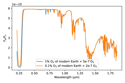
Figure 1: Simulated spectra of the two Proterozoic Earth-like scenario considered in this study.

Finally, in the final reports for HabEx and LUVOIR, concerns have been raised about the potential for degenerate solutions between O₃ and other chemical compounds within the UV wavelength range. In particular, SO₂ and H₂S show strong absorption features close to that of the ozone (Fig. 2). A closer look reveals that the features do not overlap with each other, signaling that degeneracy on the detection of O₃ is possible but not likely. To test this assumption, we included SO₂ as free parameter of the retrieval to see if we would detect it at a modest spectral resolution ($R=7$) in any of the studied cases.

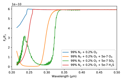
Figure 2: Absorption features of different gases in the UV wavelength band. In particular, O₃, SO₂, and H₂S absorption features are compared.

In all scenarios, we study the impact of including and excluding the UV and the NIR portion of the reflected light spectra in the retrieval. In this work, we set the “UV” wavelengths to $0.2/0.25-0.4\ \mu$m, the “VIS” wavelengths to $0.4-1.0\ \mu$m and the “NIR” wavelengths to $1.0-1.8\ \mu$m, and adopt a baseline spectral resolution of R$=$7, R$=$140, and R$=$40 for the UV, VIS, and NIR bands, respectively. These assumptions are approximately consistent with the large mission studies (Roberge & Moustakas, 2018; Gaudi et al., 2020).

Figure 3: Simulated data and best fit retrievals for the Proterozoic Earth-like scenario with 1% of Modern Earth O₂. VIS/UV/NIR spectrum predicted when fitting: VIS data only (blue curve), UV+ VIS data only (orange curve, same as blue curve, except in the UV), VIS + NIR data only (green curve), UV + VIS + NIR data only (red curve, same as green curve, except in the UV).

Lastly, to simulate the error associated to each of the data points, we considered the maximum value of the spectrum and we divided it by the desired S/N, 20 in this study. This effectively assumes that the noise is dominated by the background and not the planet, likely valid for spectroscopy of terrestrial planets (e.g., Hu et al., 2021). In the UV band, this corresponds to an average S/N=9 for the 1% O₂ scenario and S/N=12 for the 0.1% O₂ scenario. We then added a Gaussian deviation to the data to simulate the random realization of the observation.

3 Results

In this section, we present the results of the retrieval process applied to the two scenarios presented in Sec. 2.2.

3.1 1% of Modern Earth’s O₂

The retrieval results are reported in Tab. 2, and the posterior distributions are shown in Appendix A. The simulated data and the best-fit spectra are shown in Figure 3.

Table 2: Atmospheric parameters used to simulate the Proterozoic Earth-like scenario (1% of Modern Earth O₂) and the retrieval results. The error bars of the retrieval median results correspond to the 95% confidence interval (i.e., 2$\sigma$). NOTE - parameters highlighted with the asterisk are derived from the other free parameters. Color code: green strongly constrained within 3$\sigma$, orange weakly constrained within 3$\sigma$, and red not constrained or outside 3$\sigma$.

Parameter	Input	VIS	UV$+$VIS	VIS$+$NIR	UV$+$VIS$+$NIR
$Log(P_{0})$ [Pa]	$5.00$	$9.76^{+1.15}_{-1.18}$	$9.78^{+1.15}_{-1.25}$	$5.45^{+0.67}_{-0.52}$	$5.32^{+0.64}_{-0.41}$
$Log(P_{top,H_{2}O})$ [Pa]	$4.85$	$3.47^{+3.65}_{-3.19}$	$3.48^{+3.74}_{-3.30}$	$5.09^{+0.65}_{-0.52}$	$4.96^{+0.55}_{-0.36}$
$Log(D_{cld,H_{2}O})$ [Pa]	$4.30$	$3.61^{+3.88}_{-3.34}$	$3.79^{+3.93}_{-3.57}$	$4.65^{+0.69}_{-0.58}$	$4.52^{+0.56}_{-0.43}$
$Log(CR_{H_{2}O})$	$-3.00$	$-5.67^{+5.20}_{-5.83}$	$-5.74^{+5.45}_{-5.93}$	$-5.06^{+2.19}_{-4.40}$	$-4.79^{+1.92}_{-4.02}$
$Log(VMR_{H_{2}O})$	$-2.01$	$-7.37^{+0.26}_{-0.28}$	$-7.35^{+0.26}_{-0.28}$	$-2,28^{+0.55}_{-0.56}$	$-2.12^{+0.42}_{-0.44}$
$Log(VMR_{CH_{4}})$	$-4.30$	$-7.74^{+0.57}_{-5.77}$	$-7.64^{+0.54}_{-5.79}$	$-4.53^{+0.54}_{-0.73}$	$-4.37^{+0.39}_{-0.62}$
$Log(VMR_{SO_{2}})$	$-$	$-$	$-11.02^{+2.19}_{-2.80}$	$-$	$-8.71^{+0.83}_{-1.42}$
$Log(VMR_{CO_{2}})$	$-3.40$	$-$	$-$	$-5.94^{+2.92}_{-3.88}$	$-5.75^{+2.79}_{-3.84}$
$Log(VMR_{O_{2}})$	$-2.71$	$-8.54^{+2.73}_{-5.13}$	$-8.44^{+2.73}_{-5.10}$	$-3.84^{+1.77}_{-5.94}$	$-2.61^{+0.65}_{-6.14}$
$Log(VMR_{O_{3}})$	$-6.30$	$-9.61^{+3.48}_{-4.19}$	$-6.11^{+0.16}_{-0.19}$	$-7.73^{+1.75}_{-2.36}$	$-6.32^{+0.24}_{-0.26}$
$Log(VMR_{N_{2}})^{*}$	$-0.005$	$-0.01^{+0.01}_{-0.01}$	$-0.01^{+0.01}_{-0.01}$	$-0.01^{+0.01}_{-0.01}$	$-0.01^{+0.01}_{-0.01}$
$A_{g}$	$0.2$	$0.54^{+0.43}_{-0.50}$	$0.51^{+0.47}_{-0.48}$	$0.25^{+0.38}_{-0.24}$	$0.22^{+0.39}_{-0.21}$
$Log(g\ [cgs])$	$2.99$	$3.05^{+0.01}_{-0.01}$	$3.05^{+0.01}_{-0.01}$	$2.99^{+0.02}_{-0.02}$	$3.00^{+0.02}_{-0.02}$
$\mu^{*}$	$27.93$	$28.01^{+0.01}_{-0.01}$	$28.01^{+0.01}_{-0.01}$	$27.97^{+0.03}_{-0.13}$	$27.95^{+0.04}_{-0.12}$

We run ExoReL^ℜ on the simulated data while considering different combination of the wavelength band probed. Starting with the VIS band only, we decided not to fit for SO₂ and CO₂ as the spectral features of these gasses are present in UV and NIR. By inspecting the posterior distribution functions (PDFs) (blue model of Fig. 7), the solution on which the retrieval process converged is not compatible with the true values used to synthesize the data in the first place. Even though the code has been able to identify the background gas, i.e. N${}_{2}-$dominated atmosphere, it is not able to constrain the rest of the atmospheric components. The clouds parameters are not constrained at all, showing a flat posterior. This is not surprising as we exposed the weaknesses of considering the VIS band alone in the context of the characterization of the reflected light for small rocky planets in our previous work (Damiano & Hu, 2022).

Adding the UV band to the VIS gives information on the O₂ and O₃ absorption. Looking at the PDFs (orange model of Fig. 7), it is possible to see that surface and clouds parameters are still not correctly constrained. However, by inspecting the PDFs of oxygen and ozone, we find that the UV indeed provides the constraint of these two gases, and their PDFs do not show a broad posterior distribution anymore. Finally, we note that fitting SO₂, in this case, does not impact whatsoever the constraint on the O₂ and O₃ as the converged VMR value for SO₂ is equal to $-11.02^{+2.19}_{-2.80}$, practically absent.

Moving on to the VIS plus NIR case (green model of Fig. 7), the general nature of the planet is correctly identified: the background gas is correctly found, and the majority of the other gases are constrained except for CO₂ and O₃ as the VMR of CO₂ is too low to show substantial features, and because O₃ does not contain absorption bands in the VIS or NIR. Interestingly, O₂ is weakly constrained even though its VMR is quite low. This is because O₂ shows multiple but small absorption bands in the VIS and NIR wavelength range (see Fig. 1). The surface pressure of the planet has been correctly identified as well ass the surface albedo. The cloud parameters are also correctly constrained.

Finally, adding UV to VIS and NIR observations again measures the mixing ratio of O₃. By inspecting the PDFs (red model of Fig. 7), we can confirm that the nature of the planet has been correctly retrieved as the totality of the parameters converged to the true values. Also in this case, SO₂ does not impact the convergence of the detection of O₃.

We have also performed a test to reveal effect on the retrieval when considering a different lower limit of the UV band. As it may be difficult to reach 0.2 $\mu$m, we tested the case in which the UV is defined starting from 0.25 $\mu$m. Fig. 4 shows the effect on the retrieval results of O₂ and O₃. We find that a UV wavelength range of $0.25-0.4\ \mu$m would also allow measurments of O₃, as well as O₂ when the NIR coverage is also available. The retrieved PDFs for both gases are broader compared to the UV wavelength range of $0.2-0.4\ \mu$m, and the impact is more evident for O₂ as there is a strong absorption feature of O₂ between 0.2 and 0.25 $\mu$m (Fig. 2).

Finally, we noticed a minor and secondary improvement in the posterior distribution when UV is considered in addition to VIS and NIR bands. In Fig. 7, for example, the top pressure of the clouds is better constrained than the VIS+NIR case. However, when UV is considered along with VIS only (VIS vs. UV+VIS), we do not see any improvement. Moreover, we underline that the difference is only noticeable for the 1% O₂ level suggesting a correlation with the detection of O₂ in the UV and NIR bands. The improvement vanishes once the UV is cut to 250 nm or for the 0.1% O₂ level.

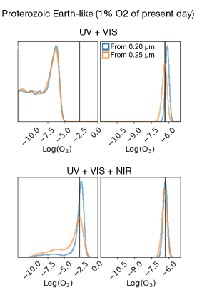
Figure 4: Effect of the lower wavelength cutoff of the UV band on the PDFs of O₂ and O₃ for the Proterozoic Earth-like with 1% of Modern Earth’s O₂. The results of the retrieval does not change appreciably. The constraints are moderately affected as the distributions are broadened. Blue curves correspond to the results shown in Tale 2, with the default 0.2 um UV lower bound.

3.2 0.1% of Modern Earth’s O₂

The Proterozoic Earth-like scenario with 0.1% of Modern Earth’s O₂ is identical to the 1% case except for the input VMR of O₂ and O₃. The retrieval results are reported in Tab. 3, and the posterior distributions are shown in Appendix B. The simulated data and the best-fit spectra are shown in Figure 5.

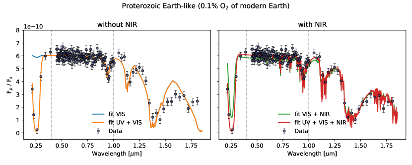
Figure 5: Simulated data and best fit retrievals for the Proterozoic Earth-like scenario with 0.1% of Modern Earth O₂. VIS/UV/NIR spectrum predicted when fitting: VIS data only (blue curve), UV+ VIS data only (orange curve, same as blue curve, except in the UV), VIS + NIR data only (green curve), UV + VIS + NIR data only (red curve, same as green curve, except in the UV).

Table 3: Atmospheric parameters used to simulate the Proterozoic Earth-like scenario (0.1% of Modern Earth O₂) and the retrieval results. The error bars of the retrieval median results correspond to the 95% confidence interval (i.e., 2$\sigma$). NOTE - parameters highlighted with the asterisk are derived from the other free parameters. Color code: green strongly constrained within 3$\sigma$, orange weakly constrained within 3$\sigma$, and red not constrained or outside 3$\sigma$.

Parameter	Input	VIS	UV$+$VIS	VIS$+$NIR	UV$+$VIS$+$NIR
$Log(P_{0})$ [Pa]	$5.00$	$9.67^{+1.25}_{-1.28}$	$9.62^{+1.28}_{-1.23}$	$5.32^{+1.07}_{-0.87}$	$5.26^{+0.78}_{-0.81}$
$Log(P_{top,H_{2}O})$ [Pa]	$4.85$	$3.18^{+3.59}_{-2.97}$	$3.60^{+3.35}_{-3.39}$	$3.88^{+1.05}_{-2.06}$	$3.84^{+0.84}_{-1.44}$
$Log(D_{cld,H_{2}O})$ [Pa]	$4.30$	$3.93^{+3.58}_{-3.61}$	$3.73^{+3.73}_{-3.51}$	$4.37^{+0.45}_{-0.61}$	$4.52^{+0.42}_{-0.40}$
$Log(CR_{H_{2}O})$	$-3.00$	$-5.98^{+5.60}_{-5.59}$	$-5.65^{+5.33}_{-5.86}$	$-8.40^{+6.29}_{-3.24}$	$-8.64^{+4.93}_{-3.08}$
$Log(VMR_{H_{2}O})$	$-2.01$	$-7.00^{+0.23}_{-0.19}$	$-6.99^{+0.21}_{-0.18}$	$-1.51^{+0.98}_{-0.59}$	$-1.54^{+0.51}_{-0.58}$
$Log(VMR_{CH_{4}})$	$-4.30$	$-10.80^{+3.05}_{-4.36}$	$-10.84^{+3.07}_{-3.55}$	$-3.98^{+1.00}_{-0.60}$	$-4.00^{+0.58}_{-0.54}$
$Log(VMR_{SO_{2}})$	$-$	$-$	$-11.31^{+1.91}_{-3.27}$	$-$	$-8.96^{+0.81}_{-1.91}$
$Log(VMR_{CO_{2}})$	$-3.40$	$-$	$-$	$-5.50^{+5.13}_{-3.64}$	$-6.96^{+4.94}_{-3.48}$
$Log(VMR_{O_{2}})$	$-3.71$	$-10.24^{+3.86}_{-4.35}$	$-10.35^{+4.11}_{-4.02}$	$-5.63^{+3.20}_{-3.26}$	$-7.48^{+3.78}_{-3.08}$
$Log(VMR_{O_{3}})$	$-6.70$	$-10.22^{+4.34}_{-4.72}$	$-6.64^{+0.13}_{-0.14}$	$-7.12^{+1.52}_{-2.70}$	$-6.68^{+0.13}_{-0.12}$
$Log(VMR_{N_{2}})^{*}$	$-0.005$	$-0.01^{+0.01}_{-0.01}$	$-0.01^{+0.01}_{-0.01}$	$-0.01^{+0.01}_{-2.61}$	$-0.01^{+0.01}_{-0.03}$
$A_{g}$	$0.2$	$0.49^{+0.42}_{-0.47}$	$0.52^{+0.45}_{-0.48}$	$0.44^{+0.31}_{-0.37}$	$0.28^{+0.38}_{-0.25}$
$Log(g\ [cgs])$	$2.99$	$3.04^{+0.01}_{-0.01}$	$3.04^{+0.01}_{-0.01}$	$3.00^{+0.01}_{-0.01}$	$2.99^{+0.1}_{-0.02}$
$\mu^{*}$	$27.92$	$28.01^{+0.01}_{-0.01}$	$28.01^{+0.01}_{-0.01}$	$27.73^{+2.76}_{-0.87}$	$27.74^{+0.21}_{-0.61}$

Also in this case, the VIS alone (blue model of Fig. 8) will not yield any significant constraints. The cloud and surface parameters are either flat or very broad. The background gas has been identified, but the chemical composition of the amotsphere shows significant biases with respect to the truth.

Adding UV data points to the visible observations results in the detection and constraints of O₃ (orange model of Fig. 8), while O₂ remains undetected by showing no constraints and a broad distribution that encompass almost the entire range probed.

Fitting the NIR band in addiction to the VIS provides constraints on the surface and cloud parameters (green model of Fig. 8). The general nature of the planet is identified with constraints on the background gas, i.e. N₂, and other minor gases like H₂O and CH₄. Like the previous scenario (1% O₂), O₂ and O₃ are not constrained.

Including the UV band in addition to VIS and NIR allows for the clear constrain of O₃ (red model of Fig. 8). All the other parameters except for CO₂ and O₂ are constrained. In this scenario, fitting for the presence of SO₂ does not impact the PDFs, highlighting once again that SO₂ and O₃ are well distinct in the UV band.

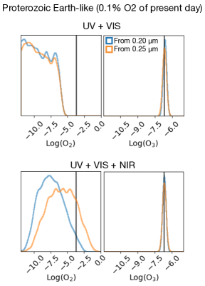
Figure 6: Similar to Fig. 4 but for the scenario with 0.1% modern Earth O₂.

Finally, repeating the retrieval process for a truncated UV band, i.e. starting from 0.25 $\mu$m rather than 0.2 $\mu$m, results in a broadening of the posterior distribution of O₃, while O₂ remains undetected (see Fig. 6).

4 Discussion

The Proterozoic period is placed in between the Archean and the Modern Earth in terms of Earth’s atmospheric evolution, and it lasted for $\sim 2$ billion years, or $\sim 40\%$ of Earth’s history. During this period, the biosphere has already been outputting O₂ from photosynthesis, but geochemical evidence indicates that atmospheric O₂ mixing ratio remained low (Planavsky et al., 2014), preventing remote-sensing detection in the visible wavelengths in similar way to modern-Earth-like planets (e.g., Feng et al., 2018; Damiano & Hu, 2022). However, due to nonlinear dependency of the photochemical O₃ mixing ratio on O₂, as well as the strong absorption of O₃, spectroscopy in the UV band may detect the O₂-O₃ biosignature via O₃ on a Proterozoic-Earth-like planet (Reinhard et al., 2017). Here we demonstrated, using rigorous spectral retrievals, that the detection of O₃ is indeed feasible, and only requires a modest spectral resolution of $R=7$ in a wavelength range of $0.25-0.4\ \mu$m.

This thus gives us a compelling science case for spectroscopic observations in the UV ($0.25-0.4\ \mu$m) for the Habitable World Observatory. Since the atmospheric concentration of O₂ and O₃ was not sufficient to show significant absorption features in the VIS or NIR wavelength bands for a good part of Earth history, not having the capabilities of starlight suppression and spectroscopy in the UV could mean missing half of Earth-like planets with an oxygenic biosphere. As O₂ and O₃ remain the leading biosignature gases for terrestrial exoplanets of FGK stars (Meadows et al., 2018), it is vital to provide sensitivity to O₃ at low mixing ratios ($10^{-7}-10^{-6}$, corresponding to the estimated Proterozoic level), which is feasible in the UV.

We also reaffirm the importance of probing the NIR band to successfully constrain the nature of the planet. The addition of the spectra in $1-1.8\ \mu$m result in the constraints of the surface/cloud properties and, importantly, the mixing ratio of H₂O. These pieces of information are essential to establish the hydrological cycle and surface habitability of an exoplanet, upon which the biosignature interpretation would be built. We have retrieved an N₂-dominated atmosphere for all scenarios considered in this paper, but for a planet with higher CO₂ mixing ratios (e.g., the Archean Earth case in Damiano & Hu, 2022), adding the NIR band is critical for determining the planet has an N₂- rather than CO₂-dominated atmosphere. The constraints on H₂O and CO₂, which are available when the NIR spectroscopy is obtained, also help delineate any geochemical/photochemical false positive scenarios for the O₂-O₃ biosignature (see a review in Meadows et al., 2018). In the case of the 1% O₂ levels, decent (but not good, i.e., broad posterior distribution, -10.0 $\lesssim$ Log(O₂) $\lesssim$ -2.0, Fig. 7) constraints on the O₂ levels can be made with the NIR part of the spectrum along with the VIS part, lessening the need for the UV spectrum.

While not studied here, the UV part of the spectrum can be useful for studying photochemical hazes in planetary atmospheres. Observations in the UV would provide additional information on haze-rich planets such as Archean Earth (Arney et al., 2016), Titan (Trainer et al., 2006), Venus (Titov et al., 2018), and Jupiter (Anguiano-Arteaga et al., 2022)). The detectability of O₃ would not be impacted by the presence of hazes as the O₃ absorption shows as a sharp edge in the UV while the haze absorption typically creates a slope in the continuum starting from $\sim 0.5\ \mu$m. Future studies could assess the information on photochemical hazes (e.g., particle size, absorption coefficient) that could be extracted from the UV and VIS spectra.

Taking into account the results of this work and the previous ones (Feng et al., 2018; Damiano & Hu, 2022), it is clear that probing the VIS wavelength band alone is not sufficient for the characterization of terrestrial exoplanets as many key gases, e.g., CO₂, CH₄, and O₃ present their main absorption features in the NIR or UV part of the electromagnetic spectrum. The capabilities in the UV and NIR wavelengths should thus be evaluated as a critical component for the future missions aiming at imaging and characterizing terrestrial exoplanets, such as the Habitable World Observatory.

5 Conclusions

In this study, we have investigated the potential of ultraviolet (UV), visible (VIS), and near-infrared (NIR) observations to characterize terrestrial exoplanets like the Proterozoic Earth in the context of the direct-imaging spectroscopy in the reflected starlight. This 2-billion-year period of Earth’s history is of particular interest, as it represents an intermediate stage between the Archean and Modern Earth, when oxygenic photosynthesis had commenced but the O₂ level in the atmosphere remained lower than the modern day.

Our analysis demonstrates the benefits of UV spectroscopy for detecting and measuring the atmospheric mixing ratios of O₃, as well as improving the measurements of O₂. Even with a modest spectral resolution of $R=7$ and an average S/N of $\sim 10$ for the UV band, the spectra can precisely measure the mixing ratio of O₃ to $\sim 10^{-7}$, without interference of other UV absorbing gases like SO₂. This makes the UV band a crucial wavelength window for the search for O₂-O₃ biosignatures on terrestrial exoplanets. Furthermore, while the O₃ detection does not rely on the NIR spectral coverage, the NIR band would provide essential habitability indicators and contextual information, including the cloud/surface pressure, atmospheric H₂O abundances, and dominant atmospheric gases (N₂ versus CO₂). Overall, it becomes clear that relying solely on the visible (VIS) wavelength band for characterizing small temperate planets can be limiting. This is because many crucial gases, such as O₃, CO₂, and CH₄, display their primary absorption characteristics in the UV (0.25 to 0.4 $\mu$m) or NIR (1.0 to 1.8 $\mu$m) regions of the electromagnetic spectrum.

Based on our findings, future direct-imaging missions aiming at finding and characterizing small rocky exoplanets (e.g., the Habitable World Observatory) should have the capability to probe both the UV and NIR bands, whenever this is feasible from the perspective of the inner working angle. This will significantly enhance our ability to detect and characterize biosignatures, thereby improving our understanding of planetary atmospheres and enhancing our search of life beyond the Solar System.

Software

ExoReL^ℜ(Damiano & Hu, 2020, 2021, 2022), Numpy (Oliphant, 2015), Scipy (Virtanen et al., 2020), Astropy (Price-Whelan et al., 2018), scikit-bio (scikit-bio development team, 2020), Matplotlib (Hunter, 2007), MultiNest (Feroz et al., 2009; Buchner et al., 2014), mpi4py (Dalcin & Fang, 2021), and corner (Foreman-Mackey, 2016).

Appendix A Scenario 1: Proterozoic Earth-like with 1% of Modern Earth’s O₂

Earth’s atmosphere has experienced multiple evolutionary stages before reaching the current state. Between the Archean and Modern epochs, another important eon in the Earth’s history is called Proterozoic. For this scenario, we simulate the reflected spectrum of an N₂-dominated atmosphere (Figs. 1 and 3). We also include H₂O, CH₄, CO₂, O₂, and O₃ as minor absorbing gases. We include a water cloud layer and a surface with albedo of 0.2. We use the synthesized data as input for ExoReL^ℜ, and Fig. 7 comprises the resulted posterior distributions of all the wavelength band combinations discussed in Sec. 2.2.

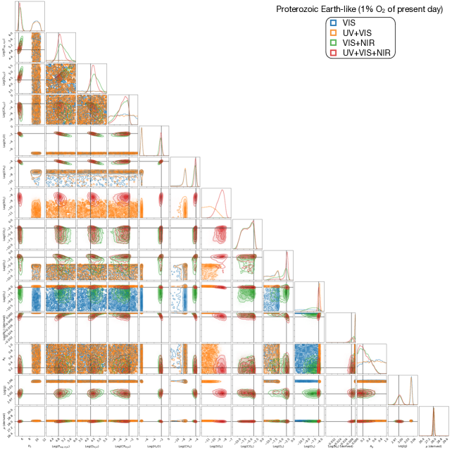
Figure 7: The full posterior distributions (corner plots) of the Proterozoic Earth-like scenario with 1% of Modern Earth’s O₂. The different cases explore a combination of different wavelength bands used for the retrieval process. The black lines in the corner plots refer to the true value used to simulate the data.

Appendix B Scenario 2: Proterozoic Earth-like with 0.1% of Modern Earth’s O₂

This scenario is similar to the previous one except for the concentration of O₂ and O₃. Therefore, we simulate, again, the reflected spectrum of a an N₂-dominated atmosphere with H₂O, CH₄, CO₂, O₂, and O₃ as minor absorbing gases (Fig. 1 and 5). We still include a water cloud layer and a surface with albedo of 0.2. The synthesized data are used as input for ExoReL^ℜ. We perform the retrieval with and without the UV and NIR part of the spectrum to explore the benefit of having a larger wavelength band in addition to the optical. The result is shown in Fig. 8.

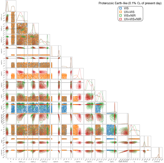
Figure 8: The full posterior distributions (corner plots) of the Proterozoic Earth-like scenario with 0.1% of Modern Earth’s O₂. The different cases explore a combination of different wavelength bands used for the retrieval process. The black lines in the corner plots refer to the true value used to simulate the data.

References

- Ahrer et al. (2023) Ahrer, E.-M., Stevenson, K. B., Mansfield, M., et al. 2023, Nature, 614, 653, doi: 10.1038/s41586-022-05590-4
- Akeson et al. (2019) Akeson, R., Armus, L., Bachelet, E., et al. 2019, arXiv e-prints, arXiv:1902.05569. https://arxiv.org/abs/1902.05569
- Alderson et al. (2023) Alderson, L., Wakeford, H. R., Alam, M. K., et al. 2023, Nature, 614, 664, doi: 10.1038/s41586-022-05591-3
- Anguiano-Arteaga et al. (2022) Anguiano-Arteaga, A., Pérez-Hoyos, S., & Sánchez-Lavega, A. 2022, in European Planetary Science Congress, EPSC2022–324
- Arney et al. (2016) Arney, G., Domagal-Goldman, S. D., Meadows, V. S., et al. 2016, Astrobiology, 16, 873
- Batalha et al. (2019) Batalha, N. E., Marley, M. S., Lewis, N. K., & Fortney, J. J. 2019, ApJ, 878, 70, doi: 10.3847/1538-4357/ab1b51
- Buchner et al. (2014) Buchner, J., Georgakakis, A., Nandra, K., et al. 2014, A&A, 564, A125, doi: 10.1051/0004-6361/201322971
- Carrión-González et al. (2020) Carrión-González, Ó., Muñoz, A. G., Cabrera, J., et al. 2020, Astronomy & Astrophysics, 640, A136, doi: 10.1051/0004-6361/202038101
- Catling & Zahnle (2020) Catling, D. C., & Zahnle, K. J. 2020, Science Advances, 6, eaax1420, doi: 10.1126/sciadv.aax1420
- Dalcin & Fang (2021) Dalcin, L., & Fang, Y.-L. L. 2021, Computing in Science & Engineering, 23, 47, doi: 10.1109/MCSE.2021.3083216
- Damiano & Hu (2020) Damiano, M., & Hu, R. 2020, AJ, 159, 175, doi: 10.3847/1538-3881/ab79a5
- Damiano & Hu (2021) —. 2021, AJ, 162, 200, doi: 10.3847/1538-3881/ac224d
- Damiano & Hu (2022) —. 2022, AJ, 163, 299, doi: 10.3847/1538-3881/ac6b97
- Damiano et al. (2020) Damiano, M., Hu, R., & Hildebrandt, S. R. 2020, AJ, 160, 206, doi: 10.3847/1538-3881/abb76a
- Feinstein et al. (2023) Feinstein, A. D., Radica, M., Welbanks, L., et al. 2023, Nature, 614, 670, doi: 10.1038/s41586-022-05674-1
- Feng et al. (2018) Feng, Y. K., Robinson, T. D., Fortney, J. J., et al. 2018, AJ, 155, 200, doi: 10.3847/1538-3881/aab95c
- Feroz et al. (2009) Feroz, F., Hobson, M. P., & Bridges, M. T. B. 2009
- Foreman-Mackey (2016) Foreman-Mackey, D. 2016, Journal of Open Source Software, 1, 24, doi: 10.21105/joss.00024
- Gaudi et al. (2020) Gaudi, B. S., Seager, S., Mennesson, B., et al. 2020, arXiv e-prints, arXiv:2001.06683. https://arxiv.org/abs/2001.06683
- Harness et al. (2021) Harness, A., Shaklan, S., Willems, P., et al. 2021, Journal of Astronomical Telescopes, Instruments, and Systems, 7, 021207
- Hu et al. (2021) Hu, R., Lisman, D., Shaklan, S., et al. 2021, Journal of Astronomical Telescopes, Instruments, and Systems, 7, 021205
- Hunter (2007) Hunter, J. D. 2007, Computing in Science & Engineering, 9, 90, doi: 10.1109/MCSE.2007.55
- JWST Transiting Exoplanet Community Early Release Science Team et al. (2023) JWST Transiting Exoplanet Community Early Release Science Team, Ahrer, E.-M., Alderson, L., et al. 2023, Nature, 614, 649, doi: 10.1038/s41586-022-05269-w
- Kaltenegger et al. (2007) Kaltenegger, L., Traub, W. A., & Jucks, K. W. 2007, The Astrophysical Journal, 658, 598
- Lupu et al. (2016) Lupu, R. E., Marley, M. S., Lewis, N., et al. 2016, AJ, 152, 217, doi: 10.3847/0004-6256/152/6/217
- Meadows et al. (2018) Meadows, V. S., Reinhard, C. T., Arney, G. N., et al. 2018, Astrobiology, 18, 630
- Mennesson et al. (2022) Mennesson, B., Bailey, V. P., Zellem, R., et al. 2022, in Society of Photo-Optical Instrumentation Engineers (SPIE) Conference Series, Vol. 12180, Space Telescopes and Instrumentation 2022: Optical, Infrared, and Millimeter Wave, ed. L. E. Coyle, S. Matsuura, & M. D. Perrin, 121801W
- National Academies of Sciences et al. (2021) National Academies of Sciences, Engineering, M., et al. 2021
- Oliphant (2015) Oliphant, T. 2015, Guide to NumPy (Continuum Press). https://books.google.com/books?id=g58ljgEACAAJ
- Palmer & Williams (1974) Palmer, K. F., & Williams, D. 1974, JOSA, 64, 1107
- Planavsky et al. (2014) Planavsky, N. J., Reinhard, C. T., Wang, X., et al. 2014, science, 346, 635
- Price-Whelan et al. (2018) Price-Whelan, A. M., Sipőcz, B. M., Günther, H. M., et al. 2018, The Astronomical Journal, 156, 123, doi: 10.3847/1538-3881/aabc4f
- Reinhard et al. (2017) Reinhard, C. T., Olson, S. L., Schwieterman, E. W., & Lyons, T. W. 2017, Astrobiology, 17, 287, doi: 10.1089/ast.2016.1598
- Roberge & Moustakas (2018) Roberge, A., & Moustakas, L. A. 2018, Nature Astronomy, 2, 605, doi: 10.1038/s41550-018-0543-8
- Robinson & Salvador (2023) Robinson, T. D., & Salvador, A. 2023, \psj, 4, 10, doi: 10.3847/PSJ/acac9a
- Rustamkulov et al. (2023) Rustamkulov, Z., Sing, D. K., Mukherjee, S., et al. 2023, Nature, 614, 659, doi: 10.1038/s41586-022-05677-y
- scikit-bio development team (2020) scikit-bio development team, T. 2020, scikit-bio: A Bioinformatics Library for Data Scientists, Students, and Developers, 0.5.5. http://scikit-bio.org
- Seager et al. (2019) Seager, S., Kasdin, N. J., Booth, J., et al. 2019, in BAAS, Vol. 51, 106
- Seo et al. (2019) Seo, B.-J., Patterson, K., Balasubramanian, K., et al. 2019, in Society of Photo-Optical Instrumentation Engineers (SPIE) Conference Series, Vol. 11117, Society of Photo-Optical Instrumentation Engineers (SPIE) Conference Series, 111171V
- Spergel et al. (2015) Spergel, D., Gehrels, N., Baltay, C., et al. 2015, arXiv e-prints, arXiv:1503.03757. https://arxiv.org/abs/1503.03757
- Titov et al. (2018) Titov, D. V., Ignatiev, N. I., McGouldrick, K., Wilquet, V., & Wilson, C. F. 2018, Space Sci. Rev., 214, 126, doi: 10.1007/s11214-018-0552-z
- Trainer et al. (2006) Trainer, M. G., Pavlov, A. A., Dewitt, H. L., et al. 2006, Proceedings of the National Academy of Science, 103, 18035, doi: 10.1073/pnas.0608561103
- Trauger & Traub (2007) Trauger, J. T., & Traub, W. A. 2007, Nature, 446, 771
- Turnbull et al. (2006) Turnbull, M. C., Traub, W. A., Jucks, K. W., et al. 2006, The Astrophysical Journal, 644, 551
- Virtanen et al. (2020) Virtanen, P., Gommers, R., Oliphant, T. E., et al. 2020, Nature Methods, 17, 261, doi: 10.1038/s41592-019-0686-2
- Young (2009) Young, G. M. 2009, Proterozoic Climates, ed. V. Gornitz (Dordrecht: Springer Netherlands), 836–839. https://doi.org/10.1007/978-1-4020-4411-3_197